Neural Forecasting at Scale

Abstract

We study the problem of efficiently scaling ensemble-based deep neural networks for multi-step time series (TS) forecasting on a large set of time series. Current state-of-the-art deep ensemble models have high memory and computational requirements, hampering their use to forecast millions of TS in practical scenarios. We propose N-BEATS(P), a global parallel variant of the N-BEATS model designed to allow simultaneous training of multiple univariate TS forecasting models. Our model addresses the practical limitations of related models, reducing the training time by half and memory requirement by a factor of 5, while keeping the same level of accuracy in all TS forecasting settings. We have performed multiple experiments detailing the various ways to train our model and have obtained results that demonstrate its capacity to generalize in various forecasting conditions and setups.

[inst1]organization=University of Sherbrooke,city=Sherbrooke, state=QC, country=Canada [inst2]organization=Unity Technologies, Labs,city=Montreal, state=QC, country=Canada [inst3]organization=Laplace Insights,city=Sherbrooke, state=QC, country=Canada

1 Introduction

In the past few years, abundant evidence has emerged suggesting that deep neural networks (DNN) constitute an effective modeling framework for solving time series (TS) forecasting problems. DNN models have been shown to produce state-of-the-art forecasts when large homogeneous datasets with multiple observations are available [1]. The success of DNN is largely accounted for by two factors: (i) the cross-learning on multiple time-series [3, 4, 5] and (ii) the use of over-specified large capacity ensemble models. However, the high computational requirements of such models in comparison to statistical models have raised concerns regarding their applicability in practical scenarios [3]. Indeed, the deployment of a reliable DNN with an automatic training procedure is far more challenging because of this cost and other factors such as optimal architecture and hyperparameter tuning which various authors discused in previous studies [10, 11]. These factors can be summarized by the following.

The need to render these methods more efficient has been pointed out multiple times [3, 12] and is one of the core challenges that must be solved to democratize their use. Currently, they require much time, specialized hardware and energy to train and deploy. Besides their model size, which can render their use cumbersome, re-training these models at every forecast for different TS is not viable for most organizations given their training time. Reducing memory requirements and computational cost, as well as offering model that are “ready-to-use” once trained are key aspects to improve upon to make these model more accessible to smaller organizations who neither have the money nor the data to support frequent retraining.

Only recently has some work been done to evaluate how to generalize these models to multiple types of TS when trained on public datasets that cover various TS settings while maintaining an acceptable level of accuracy within a zero-shot regime [13], i.e. to train a neural network on a source TS dataset and deploy it on a different target TS dataset without retraining, which provides a more efficient and reliable solution to forecast at scale than its predecessor even in difficult forecasting conditions, or in a few-shot learning regime, i.e., by fine-tuning the model to the target dataset of interest [14, 15]. In the ensemble case, the cost of runing these models is amplified since most of the current top-performing models rely on independent training of ensemble members. Producing forecasts with a small ensemble size without affecting accuracy is of great interest for smaller organization.

On the other hand, there are plentiful examples of successful deployment of neural networks in large-scale TS forecasting. It appears that the benefits of using such models in practice definitely outweigh the associated costs and difficulties [16]. First, such models are scalable: a neural TS forecasting model usually performs better as the scale of the data used to train it increases. This has been observed in various TS competitions [3, 17, 18]. Second, they can be reusable: we can reuse a model to produce forecasts over multiple TS [13] not observed during training faster and produce forecast in real-time. They also offer flexibility: It is typicaly easier to adjust a DNN-based model for handling missing values [19], adjusting its parameters based on custom business/scientific objectives [20] or considering multi-modal (various source and representation of data such as text, video, etc.) within a single end-to-end model [21].

These benefits made neural TS forecasting models popular and even mainstream in various settings. In fact, the prevalent use of neural networks manifests a paradigm shift in data-driven forecasting techniques, with fully-automated models being the de-facto standard in organizations that that can afford DNN based forecasting workflows. Many examples of DNN for TS exist. Some of the largest online retail platforms are using neural networks to forecast product demand for millions of retail items [22, 23]. AutoML solutions with heavy use of DNNs like [24] are being used in various settings and have been demonstrated to be very competitive [3] with almost no human involvement. Some companies that need to allocate a large pool of resources in different environments are using neural networks to anticipate required resources for different periods of the day [25, 26]. Large capital markets companies are using neural networks to predict the future movement of assets [27] via a process that links the trade-generating strategies with notifications and trade automation from these forecasts. However, these approaches are often not accessible to smaller organization because of their cost to opperate. We propose to tackle the problems within a single approach to facilitate the use of DNN for TS forecasting at scale.

2 Related Work

TS forecasting models: Traditional local, univariate models for TS forecasting include the autoregressive integrated moving average (ARIMA) model [30], exponential smoothing methods (HOLT, ETS, DAMPED, SES) [31, 4] decomposition-based approaches, including the THETA model [32], and autoregressive (AR) models with time-varying coefficients as in [33, 34]. Global univariate TS models that rely on deep neural networks (DNNs) have been proposed recently as alternatives to these models such as DEEP-STATE [35], DEEP-AR [22] and more recently Transformer-based models [36, 37]. In contrast to the traditional approaches, they can be trained with multiple independent TS simultaneously and handle non-stationary TS without preprocessing steps. One of the key difference between these two class of model is are how they approach the forecasting problem. Traditonal models typically learn from TS locally, by considering each TS as a separate regression task and fitting a function to each (local model) whereas DNNs do so by fitting a single function to multiple TS (global model) [16].

Some concerns have been raised regarding machine learning (ML) publications claiming satisfactory accuracy without adequate comaprison with the well-established statistical baselines and using inappropriate criteria often leading to misleading results [38]. It is inspiring to see that recent ML publications such as [35, 22, 39] have largely solved these problems by following more rigorous evaluation protocols and baseline comparisons.

Ensemble methods: Combining multiple models is often a more straightforward strategy to produce accurate forecasts than finding the best parameterization for one particular model [40, 41]. Recently, both M4 and M5 forecasting competitions have empirically confirmed the accuracy of ensemble methods [17, 3]. Notable instances of model for univariate TS forecasting include that use this method FFORMA [2] (second entry in M4), ES-RNN [42] (first entry in M4) and subsequently N-BEATS [39]. Because they use ensembling, these models, especially N-BEATS, have high computational and memory complexities, which require specialized infrastructure to accelerate their training and store the trained models [4]. For example, the full N-BEATS models consists of 180 individual models. It takes around 11’755 hours to train on the full M4 dataset using 1 NVIDIA GTX 2080Ti GPU. Furthermore, the total size of the models in ensemble is 160 GB, which, depending on the number of training logs and saved snapshots of the model, can increase to over 450 GB. In comparison, the Theta method takes around 7 min to do the same.

N-BEATS: The overall N-BEAT model [39] is designed to apply signal decomposition of the original TS similar to the “seasonality-trend-level” approach of [43] but using a fully connected neural networks organized into a set of blocks. Each blocks applies a decomposition of the signal it is given as input and make a forecast from this signal and pass the reminder of the signal to the other block. Beside the parmaterization of each block, one as to specify the number of past observations all blocks must consider which we refer as the lookback windows. When trained on large datasets, N-BEATS is trained with a bagging proeceduce [44] on various lookback windows, losses, and subpopulations to produce an ensemble of models. All of these models are independently trained and inflate the parameter size of the ensemble and thus the time to train the complete model.

Hence, the major issues of using these model at scale come down to parameter size of the model, time to train the model and whether or not we can offset the operating costs of DNN based forecasting workflows for ensemble models. This paper seek to reduce the computational complexity gap between classical and neural TS models by proposing a more memory- and computation -efficient version of the N-BEATS model [39]. Our approach achieves this by re-formulating the original fully-connected N-BEATS architecture as a single kernel convolution, which allows for training multiple models, each with different lookback windows, in parallel on the same GPU while sharing most of the parameters in the network. This leads to reduced ensemble training time and memory footprint as well as reduced ensemble model size, which positively affects the costs of training, querying and storing the resulting ensemble without compromising its accuracy.

Our contributions can be summarized as follows:

1. We introduce N-BEATS(P), a multi-head parallelizable N-BEATS architecture that permits the simultaneous training of multiple global TS models. Our model is twice as fast as N-BEATS, has 5 times fewer parameters than its predecessor, and performs at the same level of accuracy on M4 dataset than N-BEATS and generalize well in other TS forecast condition.

2. Our model is faster to train and more accurate than the top-scoring models of the M4 competition (ES-RNN [42] FFORMA [2]).

The remainder of this paper is organized as follows. Section 3 describes the univariate TS forecasting problem. Section 4 presents our modeling approach. Section 5 outlines empirical evaluation setup and our results. Finally, Section 6 presents our conclusions.

3 Problem Statement

We consider the univariate point forecasting problem in discrete time where we have a training dataset of $N$ TS, $\mathscr{D}_{\mathrm{train}}=\{\textbf{X}^{(i)}_{1:T_{i}}\}_{i=1}^{N}$ and a test dataset of future values of these TS $\mathscr{D}_{\mathrm{eval}}=\{\textbf{Y}^{(i)}_{T_{i}+1:T_{i}+H}\}_{i=1}^{N}$. The task is to forecast future values of the series, $\textbf{{Y}}^{(i)}_{T_{i}+1:H}\in\mathbb{R}^{H}$, given a regularly-sampled sequence of past observations, $\textbf{X}^{(i)}_{1:T_{i}}\in\mathbb{R}^{T^{(i)}}$. We use the bold notation to define vectors, matrix and tensor. To solve the task, we define a forecasting function $f_{\theta}:\mathbb{R}^{l}\rightarrow\mathbb{R}^{H}$, parameterized with a set of learnable parameters $\theta\in\Theta\subset\mathbb{R}^{M}$ where $l\leq T_{i}$ The parameters of the forecasting function can be learned using an empirical risk minimization framework based on the appropriate samples of forecasting function inputs, $\textbf{Z}_{\textrm{in}}\in\mathbb{R}^{l}$, and outputs, $\textbf{Z}_{\textrm{out}}\in\mathbb{R}^{H}$, taken from the training set:

$$\widehat{\theta}=\arg\min_{\theta\in\Theta}\sum_{\textbf{Z}_{\textrm{in}},\textbf{Z}_{\textrm{out}}\in\mathscr{D}_{\mathrm{train}}}\mathcal{L}(\textbf{Z}_{\textrm{out}},f_{\theta}(\textbf{Z}_{\textrm{in}}))$$ (1)

A few remarks are in order regarding the selection of the model input window size $l$. The optimal choice of $l$ is highly data-dependent. In terms of general guidelines, TS with a swiftly changing generating process [45] will favor small values of $l$, as historical information quickly becomes outdated. TS with long seasonality periods will favor larger $l$, as observing at least one and maybe a few seasonality periods may be beneficial for making a more informed forecast. Obviously, several conflicting factors can be at play here and finding a universally optimal solution for all TS does not seem viable. Therefore, $l$ can be treated as a hyperparameter selected on a TS-specific validation set. A more productive and accurate solution would entail using an ensemble of several models, each trained with its own $l$, as in [39]. However, this solution tends to inflate the ensemble size, and that is the problem we aim to address in this paper. In general, increasing the diversity of an ensemble [46] with different forecasting models usually results in the inflation of the ensemble size and computational costs. Therefore, we focus on providing a solution to more effectively parallelize training of the N-BEATS ensemble, which is obviously applicable to situations other than using multi-$l$ ensembles.

4 Model

4.1 Model architecture

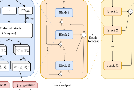
Figure 1: Illustration of the proposed model. The basic block consists of multi-head and multi-output fully connected (FC) layers with ReLU non-linear activations, where some layers are shared between the $W$ models. Each block input $\textbf{X}_{l}\in\mathbb{R}^{N\times L\times W}$ contains the same input signal at different lookback windows $l_{1}\cdots l_{W}$, where for each of the $W$ representations of the signal, missing values are padded with 0. The multi-output part of the block consists of $W$ independent layers (represented by the blue cube in the figure) that predict basis expansion coefficients both forward $\theta^{f}_{l_{w}}$ (Forecast) and backward $\theta^{b}_{l_{w}}$ (Backcast) for each of the $W$ models. A stack can have layers with shared $g^{b}_{l_{w}}$ and $g^{f}_{l_{w}}$. Forecasts are aggregated by summing over all partial forecasts of each block, enabling us to retrieve which block had the most impact in making the forecast. Parallelization is achieved by forcing head layers of each block to have the same input size, by using mask layers in the input layer to consider only the $T_{w}$ first observations of input signals and reshaping the tensor to force computation in parallel instead of sequentially applying computation in a loop for each of the $W$ models.

The basic building block of the proposed model has a multi-head architecture and is depicted in Fig. 1 (left). Each $\ell$-th block can take as input up to $W$ input signals $\textbf{x}_{l_{w}}^{(\ell)};w\in\{1,\ldots,W\}$ of the same TS with different lookback windows $\boldsymbol{l}=[l_{1},\cdots l_{W}]$, and generates two output vectors for each of the input signals provided: the backcast signal $\tilde{\textbf{x}}_{l_{w}}^{(\ell)}$ of length $l_{w}$ and the forecast signal $\tilde{\textbf{y}}_{l_{w}}^{(\ell)}$ of length equals to the forecast horizon $H$. We set each $l_{w}$ to a multiple of $H$ ranging from $2H$ to $7H$. $\tilde{\textbf{x}}_{l_{w}}^{(\ell)}$ is fed to the next block for its input and $\tilde{\textbf{y}}_{l_{w}}^{(\ell)}$ is added to the previous forecast from the previous block. Internally, the basic building block is divided into four parts.

The first part consists of $W$ independent FC input layers that project the signal into a fixed higher-dimensional representation $\textbf{z}_{l_{w}}^{(\ell)}\in\mathbb{R}^{+}$. This is done by mapping the $w$-th model with $\phi_{w}:\mathbb{R}^{l_{w}}\rightarrow\mathbb{R}^{+}$ such as $\boldsymbol{z}_{l_{w}}^{(\ell)}=\operatorname{\textsc{FC}}_{l_{w}}(\boldsymbol{x}_{l_{w}}^{(\ell)})$. To achieve parallelization in practice, we do this mapping with $\phi_{w}:\mathbb{R}^{L}\rightarrow\mathbb{R}^{+}$ where $L=max(\boldsymbol{l})$ instead and pad missing values of the $W-1$ signals with 0 that have smaller lookback windows. We set the padding to 0 for the missing values of the lookback and and make sure the FC doesn’t have bias to guarantee obtaining the same result as mapping $W$ times the input of each models sequentialy with their respective $\phi_{w}$.

The second part consists of a shared FC stack that takes as input the TS representation produced in the first part and outputs forward $\theta_{l_{w}}^{f,(\ell)}$ and backward $\theta_{l_{w}}^{b,(\ell)}$ predictors of expansion coefficients for each of the $W$ lookback periods.

The third part consists of the $W$ independent backward $g_{l_{w}}^{b,(\ell)}$ and forward $g_{l_{w}}^{f,(\ell)}$ basis layers that take as input their respective forward $\theta_{l_{w}}^{f,(\ell)}$ and backward $\theta_{l_{w}}^{b,(\ell)}$ expansion coefficients, projecting them over basis functions to produce the backcast $\tilde{\textbf{x}}_{l_{w}}^{(\ell)}\in\mathbb{R}^{L}$ and the forecast $\tilde{\textbf{y}}_{l_{w}}^{(\ell)}\in\mathbb{R}^{H}$.

This approach allows us to parallelize the computation of the forecast by considering an input $\textbf{X}\in\mathbb{R}^{N\times L\times W}$ and producing output $\tilde{\textbf{Y}}\in\mathbb{R}^{N\times H\times W}$ and obtain $W$ forecasts for $N$ TS simulatenously for each of the $W$ lookback windows.

These opperations are repeated iteratively over all blocks across all stacks of the model. Thus, the computation of the forecast and backcast for the $\ell$-th block given the $w$-th signal, is described by the following equations:

$$\textbf{z}^{(\ell)}_{l_{w}}=\operatorname{\textsc{FC}}(\operatorname{\textsc{FC}}(\cdots(\operatorname{\textsc{FC}}_{\ell,l_{w}}(\textbf{x}_{l_{w}}^{(\ell)})$$ (2)

$$\boldsymbol{\theta}_{l_{w}}^{f,(\ell)}=\operatorname{\textsc{FC}}_{l_{w}}^{f}(\textbf{z}^{(\ell)}_{l_{w}})$$ (3)

$$\boldsymbol{\theta}_{T_{w}}^{b,(\ell)}=\operatorname{\textsc{FC}}_{l_{w}}^{b}(\textbf{z}^{(\ell)}_{l_{w}})$$ (4)

$$\tilde{\textbf{y}}_{l_{w}}^{(\ell)}=g_{l_{w}}^{b,(\ell)}(\boldsymbol{\theta}_{l_{w}}^{f,(\ell)})=\sum_{i=1}^{\text{dim}\left(\boldsymbol{\theta}_{l_{w}}^{f,(\ell)}\right)}\boldsymbol{\theta}_{i,l_{w}}^{f,(\ell)}\textbf{v}_{i,l_{w}}^{f,(\ell)}$$ (5)

$$\tilde{\textbf{x}}_{l_{w}}^{(\ell)}=g_{l_{w}}^{f,(\ell)}(\boldsymbol{\theta}_{T_{w}}^{b,(\ell)})=\sum_{i=1}^{\text{dim}\left(\boldsymbol{\theta}_{l_{w}}^{b,(\ell)}\right)}\boldsymbol{\theta}_{i,T_{w}}^{b,(\ell)}\textbf{v}_{i,T_{w}}^{b,(\ell)}$$ (6)

Here, $\operatorname{\textsc{FC}}$ corresponds to a fully connected layer with ReLU non-linearity activation [47], and $\textbf{v}_{i,l_{w}}^{f,(\ell)}$ and $\textbf{v}_{i,l_{w}}^{b,(\ell)}$ are forecast and backcast basis vectors for the $\ell$-th block. These vectors can either be chosen to be learnable parameters or can be set to specific functional forms that are fixed prior to training the model. In Eq. 6, the number of time FC is applied is based on the number of layer and is part of the specification of the model.

Eqs.2-6 are then repeated iteratively for all blocks, following the same architecture topology as N-BEATS [39]. The individual blocks are stacked using two residual branches. The first branch, illustrated in Fig. 1 (middle), runs over the backcast signal produced by each block and iteratively decomposes the initial TS signal such that the subsequent block consider the residual of its preceding block. The second branch, illustrated in Fig. 1 (right), aggregates the partial forecast of each block. These operations are described by the following equations:

$$\textbf{x}_{l_{w}}^{(\ell+1)}=\textbf{x}_{l_{w}}^{(\ell)}-\tilde{\textbf{x}}_{l_{w}}^{(\ell)}$$ (7)

$$\tilde{\textbf{y}}_{l_{w}}=\sum_{\ell}\tilde{\textbf{y}}_{l_{w}}^{(\ell)}$$ (8)

4.2 Generic and Interpretable Model Version

Multiple versions of this approach can be provided to parameterize each of the $W$ models. For instance, both the generic and interpretable versions of N-BEATS proposed in [39] are compatible with our model. We will briefly describe these two extensions; we refer the reader to the original paper for more details [39].

The generic architecture: in this version, $g_{l_{w}}^{b}$ and $g_{l_{w}}^{f}$ are specified as a linear projection of the previous layer output such that the outputs of the $\ell$-th block are described as follows:

$$\tilde{\textbf{y}}_{l_{w}}^{(\ell)}=\textbf{V}_{l_{w}}^{f,(\ell)}\boldsymbol{\theta}_{l_{w}}^{f,(\ell)}+\textbf{B}_{l_{w}}^{f,(\ell)}\quad\tilde{\textbf{x}}_{l_{w}}^{(\ell)}=\textbf{V}_{l_{w}}^{b,(\ell)}\boldsymbol{\theta}_{l_{w}}^{b,(\ell)}+\textbf{B}_{l_{w}}^{b,(\ell)}$$ (9)

where $\textbf{V}_{l_{w}}^{f,(\ell)}\in\mathbb{R}^{H\times dim\left(\boldsymbol{\theta}_{l_{w}}^{f,(\ell)}\right)}$, $\textbf{B}_{l_{w}}^{b,(\ell)}\in\mathbb{R}^{H}$ and $\textbf{V}_{l_{w}}^{b,(\ell)}\in\mathbb{R}^{L\times dim\left(\boldsymbol{\theta}_{l_{w}}^{b,(\ell)}\right)}$, $\textbf{B}_{l_{w}}^{b,(\ell)}\in\mathbb{R}^{L}$ are basis vectors learned by the model, which can be taught as waveforms. Because no additional constraints are imposed on the form of $\textbf{V}_{l_{w}}^{f,(\ell)}$ the waveforms learned do not have inherent structure on how they should look.

The interpretable architecture: Similar to the traditional TS decomposition into trend and seasonality found in [43, 48], trend and seasonality decomposition can be enforced in $\textbf{V}_{l_{w}}^{f,(\ell)}$ and $\textbf{V}_{l_{w}}^{b,(\ell)}$. [39] proposed to do this by conceptually separating the set blocks into two stacks such that one stack of blocks is parameterized with a trend model ($\boldsymbol{T}$) and the other with a seasonal model ($\boldsymbol{S}$). All block in a stack shared the same parameters. The trend model consists of constraining the basis function to modelize a trend signal, i.e., using a function polynomial of small degree $p$ as follows:

$$\tilde{\textbf{y}}_{l_{w}}^{(\ell)}=g_{l_{w},\textrm{trend}}^{f,(\ell)}(\boldsymbol{\theta}_{l_{w}}^{f,(\ell)})=\textbf{T}\boldsymbol{\theta}_{l_{w}}^{f,(\ell)};\textbf{T}=[\textbf{1},t,\cdots t^{p}]$$ (10)

where T is a matrix of powers of $p$. Thus the waveform extracted will follow a monotonic or a slowly varying function. The seasonal model constrains the basis function to modelize periodic functions, i.e, $g_{T_{w}}^{f,(\ell)}(\boldsymbol{\theta}_{l_{w}}^{f,(\ell)};\textbf{V}_{t,l_{w}}^{f,(\ell)})$, using Fourier series as follows:

$$\tilde{\textbf{y}}_{l_{w}}^{(\ell)}=g_{l_{w},\textrm{seas.}}^{f,(\ell)}(\boldsymbol{\theta}_{l_{w}}^{f,(\ell)})=\textbf{S}\boldsymbol{\theta}_{l_{w}}^{f,(\ell)};$$ (11)

$$\textbf{S}=[\textbf{1},cos(2\pi\textbf{t},\cdots,cos(2\pi\lfloor{H/2-1}\rfloor\textbf{t}),sin(2\pi\lfloor{H/2-1}\rfloor\textbf{t})]$$

Thus, by first (1) applying the trend model and then (2) applying the seasonal model within the doubly residual stacking topology of the model, we obtain a model that applies TS component decomposition in a similar way to than traditional decomposition approaches. Basis functions are a generalization of linear regression where we replace each input with a function of the input. Here, the polynomial and the Fourier series are functions that model uses the trend and seasonality and take as input the embedding computed from the TS at each block ant not the raw TS values. In the case of the generic version, the basis functions for the forecasts and the backast are respectively the vectors $\textbf{V}_{l_{w}}^{f,(\ell)}$ and $\textbf{V}_{l_{w}}^{b,(\ell)}$.

In any configuration of the model, estimating the parameters of the model problem is done by maximum likelihood estimation (MLE). To simplify the notation, we consider eq. 12 as the function that establishes the forecast, where $\boldsymbol{\theta}_{\operatorname{\textsc{NBEATS}}}$ is the set of all parameters of each block and $\textbf{x}^{i}_{l_{w}}$ is the $i$-th TS considered with input size of length $l_{w}$.

$$\tilde{\textbf{y}}_{l_{w}}Y{i}=\operatorname{\textsc{NBEATS}}(\textbf{x}^{i}_{l_{w}};\boldsymbol{\theta}_{\operatorname{\textsc{NBEATS}}})$$ (12)

Thus, optimizing the model consists of optimizing eq. 13. We use a stochastic gradient descent optimization with Adam [49] over a fixed set of itterations and a three-steps learning rate schedule. Here $\mathcal{L}(NBEATS(\textbf{x}^{n}_{T_{w}};\theta_{\operatorname{\textsc{NBEATS}}}),\textbf{y}^{(n)})$ corresponds to some metric function that measures the quality of the forecast to the ground truth Y. Note that we combine the losses of the forecasts of all models, using the mean values to promote cooperation between the different models. Following the same training framework as [39], we used the MAPE, MASE and SMAPE losses to build the ensemble, all of which are detailed in the following section. We refer the reader to [39] for design choice of the model and a exhaustive discussion on the parameter choice of this model. In our work we reuse the same set of parameters and do not apply hyper-parameters search at the exception of the yearly TS where our model converge to a stable results earlier (10k itterations instead of 15k).

$$\theta^{*}_{\operatorname{\textsc{NBEATS}}}=\operatorname*{argmin}_{\theta^{*}_{\operatorname{\textsc{NBEATS}}}}{\dfrac{1}{N}}\sum_{i=0}^{N}\frac{1}{W}\sum_{w=1}^{W}\mathcal{L}(\operatorname{\textsc{NBEATS}}(\textbf{x}^{i}_{l_{w}};\theta_{\operatorname{\textsc{NBEATS}}}),\textbf{y}^{i})$$ (13)

5 Experimental setup

We conducted the experimental evaluation of the forecasting methods on 6 datasets which include a total of 105’968 unique TS when combined and over 2.5 million forecasts to produce on these TS. We report the accuracy of our model on the first and dataset and consider the rest to assess the model ability to generalize in other settings. We details all datasets here and report our generalization results on zero-shot forecasting in C. The datasets are the following:

1. (public) M4: 100’000 heterogeneous TS from multiple sectors that include economic, finance, demographics and other industry used in the M4 TS competition [17, 4].

2. (public) M3: 3003 heterogeneous TS from derived from mostly from financial and economic domains [50].

3. (public) Tourism: 1311 TS of indicators related to tourism activities sampled monthly, quarterly and yearly [51, 52].

4. (public) Electricity: 370 TS of the hourly electricity usage of 370 customers over three years [53, 54].

5. (public) Traffic: 963 TS of the hourly occupancy rates on the San Francisco Bay Area freeways scaled between 0 and 1 [53, 54].

6. (proprietary) Finance: 321 TS observed between 2005-07-01 and 2020-10-16 of the adjusted daily closing price of various U.S. mutual funds and exchange traded funds traded on U.S. financial markets, each covering different types of asset classes including stocks, bonds, commodities, currencies and market indexes, or a proxy for a market index covering a larger set of financial asset than the dataset used in [55].

For the M4, M3 and Tourism datasets, target TS trajectories were specified by the competition’s organizers with each subpopulation of TS with the same frequency (Hourly, Quarterly, etc..) having its own horizon (6, 8, etc…). For the Electricity and Traffic datasets, the test was set using rolling window operation as described in A.4. For the Finance dataset, the forecast was evaluated on three rolling forecast setups by sampling the TS on different frequencies, i.e.: daily, weekly and monthly. In total there are 2’602’878 individual TS that were sampled from the 321 original ones across 3 forecast horizons. Despite the dataset being collected from proprietary data sources which we cannot redistribute, we provide the necessary details to help interested readers reconstruct the datasets in A.5. A summary of the statistical properties, forecast horizons and metadata of these dataset are presented in  A.

We trained our model on the M4 dataset on the TS each subpopulations, i.e. [Yearly, Quarterly, Monthly, Weekly, Daily, Hourly]. We replicated the results from [39] by training the two N-BEAT model variants discussed in Sec. 4.2 using the implementation provided by the original authors and with scaled TS where we divided all TS observations by the maximum values observed. This scaling was done per TS with respect to the lookback window. For our model, the scaling was done on by dividing all lookback windows by the maximum value observed over all lookback windows.

We compared the forecast accuracy of our approaches with the reported accuracy of other TS models in the M4 TS competition including FFORMA [2] and ES-RNN [42]. In reporting the accuracy of these models, we relied upon the accuracy and the pre-computed forecasts reported in their respective original paper. The statistical models were produced on R using the forecast package [56] and we measured the training time to train and produce each forecast of our model as well as the Theta method. We also relied upon the reported running time of the implementation provided in [4]. Finally, all models were compared on a naive forecast, i.e., a random walk model or a seasonally adjusted random walk, that assumes all future values will be the same as the last known one(s). This was done to assess whether the forecasts of these models are accurate in the first place.

$$MAPE(\boldsymbol{\tilde{x}},\boldsymbol{x})=\frac{100}{H}\sum_{i=1}^{H}\frac{|\boldsymbol{\tilde{x}}_{T+i}-\boldsymbol{x}_{T+i}|}{\boldsymbol{x}_{T+i}}$$ (14)

$$MASE(\boldsymbol{\tilde{x}},\boldsymbol{x})=\frac{1}{H}\frac{\sum_{i=1}^{H}|\boldsymbol{x}_{T+i}-\boldsymbol{\tilde{x}}_{T+i}|}{\frac{1}{T-m}\sum_{t=m+1}^{T}|\boldsymbol{x}_{t}-\boldsymbol{x}_{t-m}|}$$ (15)

$$SMAPE(\boldsymbol{\tilde{x}},\boldsymbol{x})=\frac{200}{H}\sum_{i=1}^{H}\frac{|\boldsymbol{x}_{T+i}-\boldsymbol{\tilde{x}}_{T+i}|}{|\boldsymbol{x}_{j}|+|\boldsymbol{\tilde{x}}_{T+i}|}$$ (16)

$$OWA(\boldsymbol{\tilde{x}},\boldsymbol{x})=\frac{1}{2}\left[\frac{SMAPE}{SMAPE_{NAIVE2}}+\frac{MASE}{MASE_{NAIVE2}}\right]$$ (17)

$$ND(\boldsymbol{\tilde{x}},\boldsymbol{x})=\frac{\sum_{i=1}^{H}|\boldsymbol{\tilde{x}}_{T+i}-\boldsymbol{x}_{T+i}|}{\sum_{i=1}^{H}|\boldsymbol{x}_{T+i}|}$$ (18)

$$MDA(\boldsymbol{\tilde{x}},\boldsymbol{x})=\frac{1}{H}\sum_{i=1}^{H}\text{sign}(\boldsymbol{\tilde{x}}_{T+i}-\boldsymbol{x}_{T})=\text{sign}(\boldsymbol{x}_{T+i}-\boldsymbol{x}_{T})$$ (19)

We evaluated the forecast accuracy using 8 standard TS metrics: the mean absolute percentage error (MAPE) used in the Tourism compeition [51], the mean absolute scaled error (MASE) [57], the scaled mean absolute percentage error (SMAPE) used in the M3 competition [50], the normalized deviation (ND) used in [22] and the mean directional accuracy (MDA). Additionally for the M4 competition, we evaluated the model on the overall weighted average (OWA) between the SMAPE and the MASE such that a seasonally-adjusted naive (NAIVE2) forecasting model obtains a score of 1.0 [4]. For instance, an OWA of 0.90 means that the forecast is on average 10% better than a NAIVE2 model with respect to both the SMAPE and MASE metrics. The MDA measures the model’s ability to produce forecasts where the trajectory follows the actual change of the TS relative to the last known value: the higher the MDA is, the better a model predicts the trend of a TS at any given time. For all other metrics, the lower the value, the better a model predicts the TS. For the M4 dataset, we only consider the OWA, the MASE and the MDA. The other metrics were used in order to compare ourselve with other methods and other datasets as detailed in C.

Eq. 14-19 describes how these metrics are computed. $\tilde{x}$ is the forecast, $x$ is the ground truth and $m$ is the time interval between successive observations considered by the organizers for each data frequency, i.e., 12 for monthly, four for quarterly, 24 for hourly and one for yearly, weekly and daily data. Without loss of generality to previous equatios $T$ is the number of point in-sample observed to make the forecastushe and $H$ is the forecast horizon.

5.1 Baseline and Benchmark

.

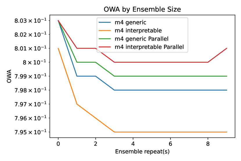
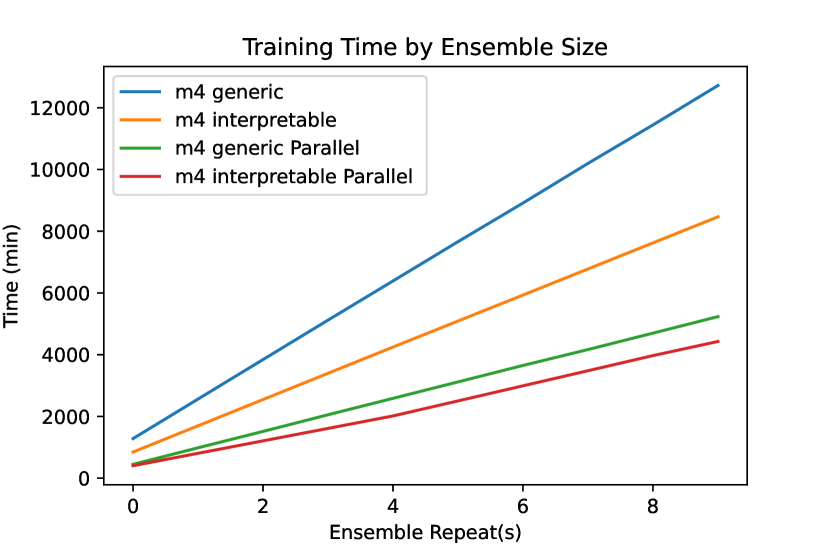
Figure 2: OWA metric (left) and Time (right) in minutes for the different N-BEATS models configurations as a function of ensemble size.

We present the results of the baseline and benchmark accuracies for the M4 dataset in Table 1. The table gives the reported accuracy of N-BEATS reported in the original papers [39], the replicated results using the publicly accessible implementation provided by the original authors along with their scaled versions [13] based upon their implementation and our model NBEATS(P). Three main conclusions can be drawn:

1. Scaling TS to allow generalization on other datasets for the N-BEATS model, as presented in [13], adds a penalty on the OWA metrics for the M4 dataset, which suggests that there is a trade-off between accuracy and generalization on other datasets for DNN-based models.

2. Figure 2 details how sensemble size has an impact on computational time to train. It can be seen that applying a bagging procedure [44] 3 to 4 times is sufficient to get an accurate ensemble for both the NBEATS and NBEATS(P) model but NBEATS(P) is more efficient the larger the ensemble size is.

3. The top-performing models do not differ significantly with respect to the coverage of the TS forecasted and the mean directional accuracy (MDA). This provides an argument that if one is mainly interested in predicting the TS variation from the forecast origin, relying on the fastest implementation of the top-performing models for a first initial prediction is a cost-effective solution.

.

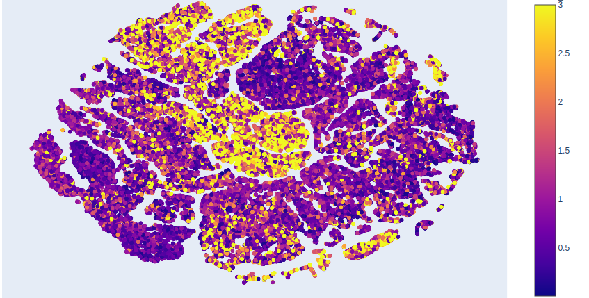
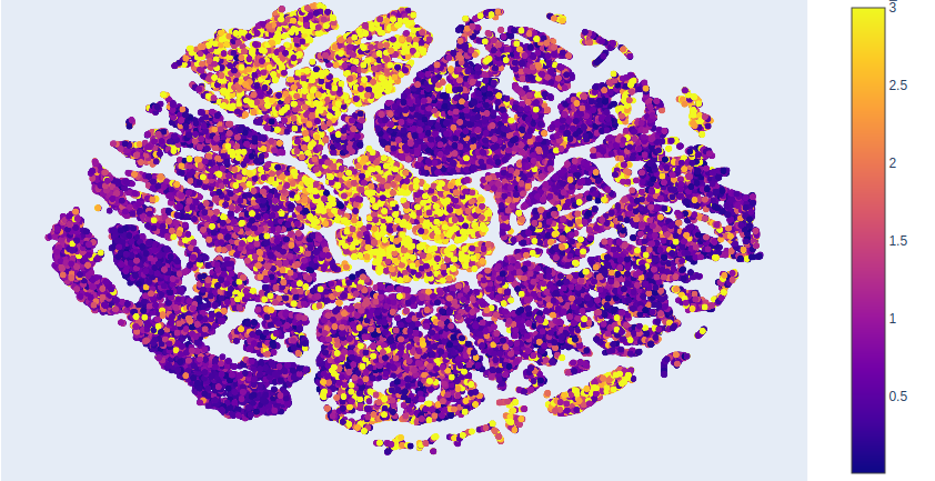
Figure 3: MASE coverage for the ES-RNN (left) and N-BEATS(i) (right) over the M4 dataset. Each point on the graphs corresponds to a single TS and the darker its color, the better the given model according to the MASE. Horizontal and vertical coordinates represent the value of the two-dimensional embedding computed with TSNE [58] from the statistical features of the series which we detail in A. All TS with MASE values over 3 where assigned the same color to facilitate visualization.

Regarding (2), we illustrate this phenomenon in fig. 3 by plotting the TSNE embedding of each series of M4 computed from the same set of features used in the FFORMA [2] by comparing the top performing model with the N-BEATS(i) model by coloring each TS with its individual MASE accuracy. We refer the reader to table.5 and [2, 59] for a detailed overview of the 42 features used and their interpretation. A details the distribution of these features over all datasets we considered. Note that there are no substantial differences between the approaches, despite some subtle regions of the graph where we can observe N-BEATS(i) performing better overall than ES-RNN.

Yearly Quarterly Monthly Others Average Coverage OWA MASE % ($<T=1.0$) MDA(%) NAIVE 1.000 1.066 1.095 1.335 1.058 40.299 3.2 NAIVE2 1.000 1.000 1.000 1.000 1.000 43.288 33.1 SNAIVE 1.000 1.153 1.146 0.945 1.078 36.095 42.7 ARIMA [30] 0.892 0.898 0.903 0.967 0.903 51.145 53.8 HOLT [60] 0.947 0.932 0.988 1.180 0.971 48.659 61.7 ETS [61] 0.903 0.890 0.914 0.974 0.908 50.987 48.6 THETA [32] 0.872 0.917 0.907 0.995 0.897 48.686 61.7 SES [31] 1.002 0.970 0.951 0.995 0.975 44.719 35.3 DAMPED [4] 0.890 0.893 0.924 1.005 0.907 49.838 61.1 COMB [4] 0.867 0.890 0.920 1.039 0.898 49.784 61.3 MLP’ [4, 62] 1.288 1.684 1.749 3.028 1.642 26.603 60.6 RNN’ [4, 62] 1.308 1.508 1.587 1.702 1.482 28.437 59.8 ProLogistica [63] 0.820 0.855 0.867 0.742 0.841 53.620 62.6 FFORMA [2] 0.799 0.847 0.858 0.914 0.838 53.418 63.7 ES-RNN [42] 0.778 0.847 0.836 0.920 0.821 53.271 63.2 N-BEATS (I) [39] 0.765 0.800 0.820 0.822 0.797 — — N-BEATS (G) [39] 0.758 0.807 0.824 0.849 0.798 — — N-BEATS (I+G) [39] 0.758 0.800 0.819 0.840 0.795 — — Ours: N-BEATS (G) [39] 0.770 0.793 0.818 0.832 0.798 55.576 64.6 N-BEATS (I) [39] 0.763 0.797 0.817 0.838 0.795 55.600 63.7 N-BEATS (I+G) [39] 0.761 0.792 0.814 0.834 0.793 55.868 64.6 N-BEATS (G) scaled [13] 0.784 0.810 0.827 0.836 0.809 54.960 64.5 N-BEATS (I) scaled [13] 0.773 0.817 0.826 0.843 0.806 54.919 63.7 N-BEATS (I+G) scaled [13] 0.778 0.814 0.824 0.836 0.806 55.109 64.4 N-BEATS parallel (G) 0.764 0.804 0.820 0.855 0.799 55.332 64.4 N-BEATS parallel (I) 0.759 0.817 0.824 0.850 0.801 54.966 63.7 N-BEATS parallel (I+G) 0.757 0.806 0.820 0.851 0.796 55.375 64.5 N-BEATS parallel (G) scaled 0.775 0.829 0.833 0.851 0.812 54.506 63.8 N-BEATS parallel (I) scaled 0.772 0.845 0.844 0.867 0.819 53.772 63.6 N-BEATS parallel (I+G) scaled 0.771 0.834 0.835 0.854 0.813 54.344 63.9

Table 1: Averaged forecasting results of the M4 competition for the evaluated models. The OWA metric is presented for each seasonal pattern observed. Forecasts from models in italics were pre-computed except for the N-BEATS models. We replicate the results with the implementation provided by the authors, e.g: N-BEATS (I) (original) vs N-BEATS (I) (our). MLP’ and RNN’ models are appended with "’" to signify that these model were trained per TS using a seasonal and trend decomposition with manual pre- and post processing steps [4]. We also considered a coverage indicator which measures the number of series that a model forecasts better than an arbitrary MASE accuracy threshold of $\tau=1.0$. We also added the MDA of the forecast.

5.2 Training Time and Number of Parameters

Table 2 presents the time to train each model accuracy as well as the average pairwise absolute percentage error correlation of the forecast residuals between ensemble members, in a way to similar to the experimental evaluation of M4 submission performed in [64]. At first glance, we see that the training time of these models be as long as multiple weeks. N-BEATS models timing are reported with a single GPU. In comparison to N-BEATS, N-BEATS(P) takes less time regardless of the variant used but the gain is observed especially for the generic architecture. Both the original approach and ours are at the same level of correlation and, while ours is slightly less diverse, it is roughly twice as efficient and achieves the same level of accuracy. We can observe that using the scaled version has little impact in terms of diversity. In our preliminary result, we also observed that there was no significant difference in terms of the TS samplers used to train N-BEATS(P) where for instance, different TS were sampled for the $W$ model.

In practice, computational time remains more than significant for training these models on a single GPU. However, we can speed up the training by training model simulatenously. If we consider N-BEATS(G) vs N-BEATS(P, G), each ensemble member trained on a single TS frequency takes on average 12 & 27 minutes, and at worst, 19 & 57 minutes respectively. N-BEATS(G)’s time is for a single lookback and thus requires 1080 ($6\text{ lookback}\times 3\text{ losses}\times 6\text{ frequencies}\times 10\text{ repeats}$) independent models to be trained whereas N-BEATS(P, G) requires only ($3\text{ losses}\times 6\text{ frequencies}\times 10\text{ repeats}$) independent models. Thus, if one would have access to 1080 GPUS, the total training time of N-BEATS(G) could be done in 20 min, but this is an unrealistic amount of ressources for most organization. Our approach cuts down that cost: given 10 GPUs, the N-BEATS(G) and a greedy schedudling of model training, it would take roughly 35h to train whereas our would only take 16h with all 10 repeats. Using 20 gpus, our model would achieve it in 8 hours whereas the previous model would take 18.

When forecasting larger amount of TS, say 1 billions monthly distinct TS, estimating the cost can be difficult. We can make a reasonable assumption that the computational time required to train a model scales linearly with the number of time series to forecast altought it takes roughly the same to train on different subpopulations or the other based on the number of itterations. Hence assuming we are using the same 3 losses and bagging procedure and it takes a single model to train the monthly TS where the number of itterations required linearly scaled from the one used in M4 (see 9) and require 75k itterations instead, it would take 1878h and 1551h for the generic and interetable version of our model on 30 GPUS. Altough a larger dataset may benefit from a deeper & wider model further inflating the cost, the number of itterations might not need to be this high. However, our approach will result in similar gain in the scenario of deeper & wider model. Regardless, training these model for everyday usage requires a lot of computational ressouce. In order for the cost to be kept low at this scale, training would need to be done less frequently and models would have to remain outdated to some extent as recent trends and structural changes in the data wouldn’t be used to update the model parameters.

To further show the performance of our model, we show in Table. 3 that one could have achieved the same average accuracy as the top M4 competitions entries by training our for approximatively 2h on a single GPU without bagging. Thus, even with minimal amount of ressources, smaller organizations can train 54 DNN-based models, each on TS of different freqencies, losses and lookback windows very fast making our model far more accessible to small organization who doesn’t have dozens of gpus available.

Since the training procedure of our approach takes roughly a fixed amount of time to train regardless of the number of TS to forecast, forecasting more TS might requires more itterations and/or more parameters for the model to capture the dynamics of these additonal TS. Therefore the training time is expected to increase the more TS we want to forecast in the training regime. However, the overall training time doesn’t increase linearly with the number of TS to forecast as increasing the number of itteration is a fixed cost and the number of itterations to train Quarterly (24K TS) or Monthly (48K TS) was the same in our setting. This leaves, the total number of itterations to train all models, the forecast horizons, the number of parameters and the number of models trained simultanously to have effect on training time.

The difference in improvement factor between parallelized generic and interpretable versions of N-BEATS(P) is due to the hidden layer sizes between the two versions. Having a higher number of hidden neurons reduce the computational gain of training multiple models conjointly as it saturate GPU usage. If we have a sufficiently expressive model without requiring too many hidden neurons, N-BEATS(P) is expected to produce accurate forecasts at a fraction of the cost. Otherwise the gain will be diminished. Regardless, these results show that ensemble diversity and accurate forecasts could have been achieved with reduction in resources and computation time.

Time (min.) Corr. (mean, std.) Time (min.) Corr. (mean, std.) Theta 7.28 $--\pm--$ ProLogistica [63] 39655 $--\pm--$ FFORMA [2]: 46108 $--\pm--$ ES-RNN [42]: 8056 $--\pm--$ N-BEATS(G) [39] 11773 $0.85\pm 0.02$ N-BEATS(G) scaled 11755 $0.84\pm 0.04$ N-BEATS(I) [39] 7437 $0.89\pm 0.02$ N-BEATS(I) scaled 6607 $0.85\pm 0.03$ N-BEASTS(I+G) [39] 19211 $0.84\pm 0.03$ N-BEATS(I+G) scaled 19170 $0.84\pm 0.03$ N-BEATS(P, G) (our) 5301 $0.87\pm 0.02$ N-BEATS(P,G) scaled (our) 6157 $0.90\pm 0.02$ N-BEATS(P, I) (our) 6990 $0.89\pm 0.03$ N-BEATS(P,I) scaled (our) 4785 $0.89\pm 0.08$ N-BEATS(P, I+G) (our) 11840 $0.88\pm 0.02$ N-BEATS(P,I+G) scaled (our) 10943 $0.89\pm 0.06$

Table 2: Time required to train to train all members of the ensemble of our models vs other and average & standard deviation of the absolute percentage correlation between ensemble members on the test sets. We include the total time to produce a forecast for the theta method for comparison. Except for Prologistica, FFORMA and ES-RNN whose training time was replicated in [4], the total time presented is with all model are for single instance and do not consider the speedup that can be achieved based when training the whole ensemble on multiple GPUs.

model name OWA (average) time to train (min) ensemble size N-BEATS (G) 0.816 419 6 N-BEATS (I) 0.815 280 6 N-BEATS parallel (G) 0.820 99 6 N-BEATS parallel (I) 0.821 134 6

Table 3: Performance of a small ensemble only trained on the MAPE loss for all lookback without bagging and time to train on a single GPU.

Given the increasing trend of top-performing models requiring ever more training time [4], training and deploying state-of-the-art models in real-case scenarios can entail high costs for organizations — costs that are avoidable. For instance, on Google’s cloud platform, the estimated cost of training N-BEATS(P) would drop to 530.11 USD$ instead of the 860.13 USD$ their price simulator gives for N-BEATS. Thus, in terms of both cost and time saved, our work provides encouraging results that suggest how multiple TS ensemble models can be accelerated without any great drawback by sharing a subset of their parameterization.

Model name # of parameters Model name # of parameters N-BEATS(G) 28’508’265’900 N-BEATS(P, G) 5’972’957’400 N-BEATS(I) 42’288’737’310 N-BEATS(P, I) 8’102’076’930 N-BEATS(I+G) 70’797’003’210 N-BEATS(P, I+G) 14’075’034’330

Table 4: Number of parameters for the whole ensemble for N-BEATS and N-BEATS (parallel) trained on the M4 dataset with 6 lookback windows.

6 Conclusion

We proposed an efficient novel architecture for training multiple TS models conjointly for univariate TS forecasting. We empirically validated the flexibility of our approach on the M4 TS datasets as well as assessing its generalizability to other domains of application, using 5 other datasets which, combined, cover over 2.5 million forecasts. We provided forecasts in various TS settings at the same level of accuracy as current state-of-the-art models with a model that is twice as fast while requiring 5 times fewer parameters than the top performing model. We highlighted both stylized facts and limitations of the performance of the model studied, in an effort to provide insights to TS practitioners for operating DNN-based models at scale. Our results suggest that training global univariate models conjointly by sharing parts of their parameterizations yield competitive forecasts in a fraction of the time and does not significantly impair either forecast accuracy or ensemble diversity.

Appendix A Dataset

Fig. 4 illustrates the difference between the statistical properties of all 6 datasets, employing the same set of TS features used in the FFORMA model [2]. We refer the reader to table.5 and [2] for a detailed overview of the 42 features used and their interpretation. As an example of the observations that can be drawn from this figure: it can bee seen that both the Electricy and Traffic datasets exhibit multiple seasonal patterns, whereas datasets like Finance exhibit large difference from other datasets in terms of high order autocorrelation (x_acf10), autoregressive conditional heteroscedasticity (archlm, garch_r2), strength of trend (trend) and high variance of the mean of observation from non-overlapping windows (stability).

Features Description Seasonal Non-Seasonsal 1 $T$ length of time series ✓ ✓ 2 trend strength of trend ✓ ✓ 3 seasonality strength of seasonality - ✓ 4 linearity Linearity ✓ ✓ 5 curvature Curvature ✓ ✓ 6 spikiness Variance of the leave-one-out variances of the remainder component in STL decomposition ✓ ✓ 7 e_acf1 first autocorrelation function (ACF) value of remainder series ✓ ✓ 8 e_acf10 sum of squares of first 10 ACF values of remainder series ✓ ✓ 9 stability sum of squares of first 10 ACF values of remainder series ✓ ✓ 10 lumpiness Variance of the means produced for tiled (non-overlapping) windows ✓ ✓ 11 entropy Spectral entropy (Shannon entropy) of the TS ✓ ✓ 12 hurst Hurst exponent from [65] ✓ ✓ 13 nonlinearity Teraesvirta modified test [66] ✓ ✓ 13 alpha $\text{ETS(A,A,N)}\hat{\alpha}$ ✓ ✓ 14 beta $\text{ETS(A,A,N)}\hat{\beta}$ ✓ ✓ 15 hwalpha $\text{ETS(A,A,A)}\hat{\alpha}$ ✓ ✓ 16 hwbeta $\text{ETS(A,A,A)}\hat{\beta}$ - ✓ 17 hwgamma $\text{ETS(A,A,A)}\hat{\gamma}$ - ✓ 18 ur_pp Test statistic based on Phillips-Perron test [67] ✓ ✓ 19 ur_kpss test statistic based on KPSS test [68] ✓ ✓ 20 y_acf1 first ACF value of the original series ✓ ✓ 21 diff1y_acf1 First ACF value of the differenced series ✓ ✓ 22 diff2y_acf1 First ACF value of the twice-differenced series ✓ ✓ 23 y_acf10 Sum of squares of first 10 ACF values of original series ✓ ✓ 24 diff1y_acf10 Sum of squares of first 10 ACF value of the differenced series ✓ ✓ 25 diff2y_acf10 Sum of squares of first 10 ACF value of the twice-differenced series ✓ ✓ 26 seas_acf1 autocorrelation coefficient at first seasonal lag - ✓ 27 sediff_acf1 first ACF value of seasonally differenced series - ✓ 28 y_pacf5 sum of squares of first 5 PACF values of original series ✓ ✓ 29 diff1y_pacf5 sum of squares of first 5 PACF values of original series ✓ ✓ 30 diff2y_pacf5 sum of squares of first 5 PACF values of twice-differenced series ✓ ✓ 31 seas_pacf partial autocorrelation coefficient at first seasonal lag ✓ ✓ 32 crossing_points number of times the time series crosses the median ✓ ✓ 33 flat_spots number of flat spots, calculated by discretizing the series into 10 equal-sized intervals and counting the maximum run length within any single interval ✓ ✓ 34 nperiods number of seasonal periods in the series - ✓ 35 seasonal_period length of seasonal period - ✓ 36 peak strength of peak ✓ ✓ 37 trough strength of trough ✓ ✓ 38 ARCH.LM ARCH.LM statistic ✓ ✓ 39 arch_acf sum of squares of the first 12 autocorrelations of $z^{2}$ ✓ ✓ 40 garch_acf sum of squares of the first 12 autocorrelations of $r^{2}$ ✓ ✓ 41 arch_r2 $R^{2}$ value of an AR model applied to $z^{2}$ ✓ ✓ 42 garch_r2 $R^{2}$ value of an AR model applied to $r^{2}$ ✓ ✓

Table 5: List of features used to compare datasets. The functions for calculating these features are implemented in the tsfeatures R package by [59]. Default values when test failed was 0.

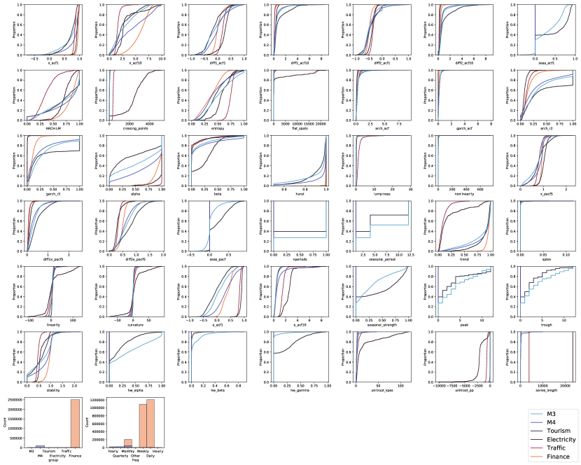
Figure 4: Cumulative distribution function plot for TS datasets over 42 statistical TS features and TS count by dataset and frequency.

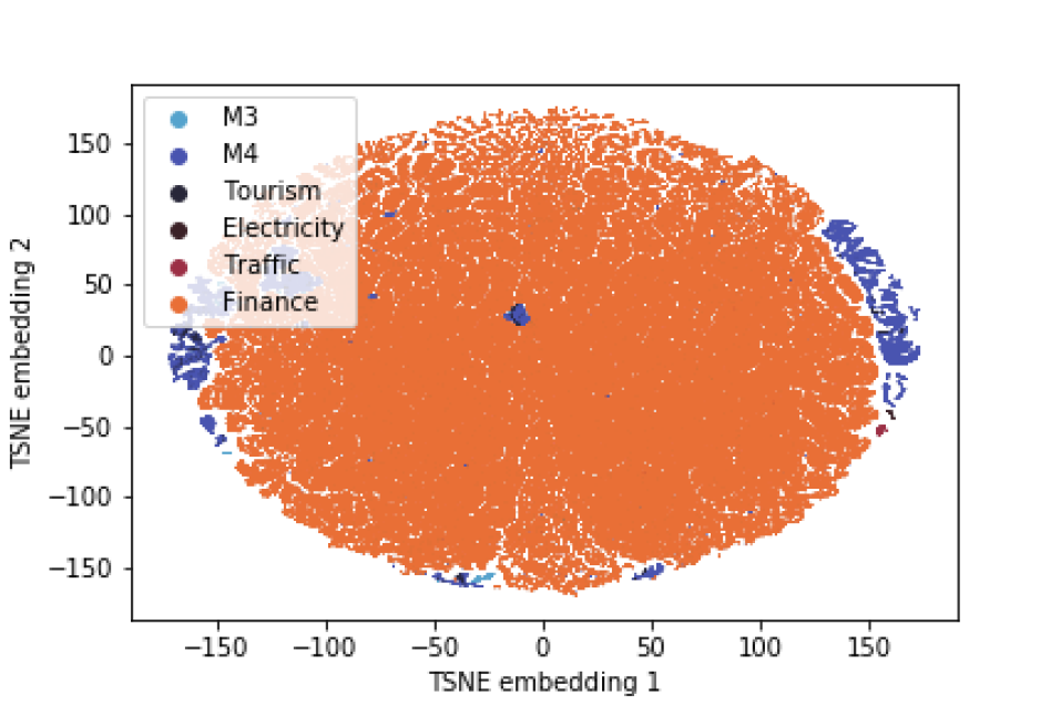
Figure 5: TSNE embedding of all TS forecasted with their different subpopulations.

All sampled TS from all datasets are summarized in Fig. 5 using the T-SNE algorithm [69]. Each point of this graph correspond to the 2-dimensional embedded space of a single TS computed from the same set of endogenous statistical features[2] . One can observe the heterogeneity of these datasets and note that the subpopulations of TS within a dataset can have high variance in their statistical properties while being similar to other subpopulations of other datasets. When considering the Finance dataset, we can see how the behavior of the 321 TS changes is heterogenou over time in comparison to the other dataset. The Electricity & Traffic TS share almost the same statistical properties as both populations of TS are concentrated in the same region of the graph.

A.1 M4 Dataset Details

Frequency/Horizon Type Yearly $(h=6)$ Quarterly $(h=8)$ Monthly $(h=18)$ Weekly $(h=13)$ Daily $(h=14)$ Hourly $(h=48)$ Total Demographic 1’088 1’858 5’728 24 10 0 8’708 Finance 6’519 5’305 10’987 164 1’559 0 24’534 Industry 3’716 4’673 10’987 164 422 0 18’798 Macro 3’903 5’315 10’016 41 127 0 19’402 Micro 6’538 6’020 10’975 112 1’476 0 25,121 Other 1’236 865 277 12 633 414 3437 Total 23’000 24’000 48’000 359 4277 414 100’000

Table 6: Composition of the M4 TS dataset: number of time series based on their sampling frequency and type.

The M4 dataset is a publicly accessible dataset that contains a large set of 100’000 heterogenous TS sampled from the ForeDeCk database for the M4 competition[17]. The database is compiled at the National Technical University of Athens and is built from multiple diverse and publicly accessible sources. It includes TS frequently encountered in business domains such as industries, services, tourism, imports/exports, demographics, education, labor & wage, government, households, bonds, stocks, insurances, loans, real estate, transportation, and natural resources & environment. TS were sampled at different frequencies [Yearly, Quarterly, Monthly, Weekly, Daily and Hourly] each with different forecast horizons, i,e, [6, 8, 18, 13, 14, 48] according to the competition organizer. Table 6 outlines the composition of the M4 dataset across domains and forecast horizons.

All TS were provided with a prepossessing scaling procedure to ensure positive observed values at all time-steps with minimum observed values greater than or equal to 10. The scaling was applied only to sampled TS whose minimum oberved value was smaller than 10 by adding a per-TS constant to all TS to ensure that the minimal values was positive. All other TS were unaltered by any preprocessing step. The dataset was subdivized into a training and a test dataset by the M4 TS competition organizers. For further details on this dataset, we refer the reader to the following: [4, 17]. We relied on the pre-computed forecasts and PI available at https://github.com/Mcompetitions/M4-methods.

A.2 M3 Dataset Details

Frequency/Horizon Type Yearly $(h=6)$ Quarterly $(h=8)$ Monthly $(h=18)$ Other $(h=8)$ Total Demographic 245 57 111 0 413 Finance 58 76 145 29 308 Industry 102 83 334 0 519 Macro 83 336 312 0 731 Micro 146 204 474 4 828 Other 11 0 52 141 204 Total 645 756 1428 174 3’003

Table 7: Composition of the M3 TS dataset: the number of TS based on sampling frequency and type.

The M3 dataset is a publicly accessible dataset that is smaller than the M4 dataset but remains relatively large and diverse. Similarly to the M4 dataset, it contains TS frequently encountered in business, financial and economic forecasting. It include yearly, quarterly, monthly, weekly, daily and hourly time series, each with different forecast horizons, i,e, [6, 8, 18, 13, 14, 48]. All series have positive observed values at all time-steps. The dataset was subdivided into a training and a test dataset by the M3 TS competition organizers. Table 7 outlines the composition of the M3 dataset across domains and forecast horizons. For further details on this dataset, we refer the reader to [50]. This dataset was considered for zero-shot forecasting, to examine a case where the target dataset is from the same domains of application but with other TS.

A.3 Tourism Dataset Details

Frequency/Horizon Type Yearly $(h=4)$ Quarterly $(h=8)$ Monthly $(h=24)$ Total Tourism 518 427 366 1311

Table 8: Composition of the Tourism TS dataset: number of time series based on sampling frequency and type.

The Tourism dataset is a publicly accessible dataset that contains TS collected by [51] from tourism government agencies and academics who had used them in previous tourism forecasting studies. The TS of this dataset are highly variable in length. It includes yearly, quarterly and monthly TS. Table. 8 details the proportion of TS from each frequency. For further detail on this dataset, we refer the reader to [51]. This dataset was considered for zero-shot forecasting, to examine a case where the target dataset comes from domains that are not present in the M4 dataset.

A.4 Electricity and Traffic Datasets Details

Electricity and Traffic [70] are two publicly available datasets from the Univeristy of California Irvine Machine Learning repository. The Electricity dataset contains the hourly electricity usage monitoring of 370 customers over three years, with some clients being added during the the observation periods creating cold-start conditions for producing some forecasts. The Traffic dataset contains TS of the hourly occupancy rates, scaled in the (0,1) range for 963 lanes of freeways in the San Francisco Bay area over a period of slightly more than a year. Both of these dataset exhibit strong seasonal patterns due to their nature and are mostly homogeneous. These two TS datasets are used de facto to evaluate the quality of DNN-based TS models as in [22, 35, 71]. We included these two datasets as a sanity check for zero-shot forecasting, to ensure that zero-shot forecasts were accurate in a setting where it is relatively easy to produce accurate forecasts.

A.5 Finance dataset

The Finance dataset contains daily closing prices of U.S. MFs and ETFs observed between 2005-07-01 and 2020-10-16 and traded on U.S. financial markets, each covering different types of asset classes including stocks, bonds, commodities, currencies and market indexes, or a proxy for a market index. The dataset was obtained through three data providers: (1) Fasttrack, a professional-grade data provider for financial TS, (2) YahooFinance API and (3) the Federal Reserve of Saint-Louis (FRED) database. Part of this dataset is proprietary, so we do not have permission to share that part publicly. However, the list of securities is given in Table. LABEL:tab:appendix_list_of_securities to help interested readers reconstruct the dataset from public data sources.

We considered this dataset in our zero-shot experiments by sampling the TS at three different frequencies [dDaily, weekly and monthly] and specifying the same forecast horizon as that of the M4 dataset. We used this dataset to present a worst-case scenario for zero-shot. First this is a case where the forecasting application is notorious for its forecasting difficulty. Moreover, the source dataset on which we train our model has at most 10K TS to train from and at worst 164 TS, which force zero-shot generalization with very few training data. Also, by sampling the TS at large scale, we emulated how zero-shot could be applied on the whole history of the TS, similar to the procedure carried out by portfolio managers and quantitative analyst to backtest the validity of their investment strategies. The TS were split into chunks of the maximum lookback period of the N-BEATS model as training sample, and $H$ steps-ahead as testing sample.

Appendix B Training setup details

Frequency/Horizon Frequency Yearly $(h=6)$ Quarterly $(h=8)$ Monthly $(h=18)$ Weekly $(h=13)$ Daily $(h=14)$ Hourly $(h=48)$ $L_{H}$ 1.5 1.5 1.5 10 10 10 Iterations N-BEATS P 10k 15k 15k 5k 5k 5k Iterations N-BEATS 15k 15k 15k 5k 5k 5k Learning rate 0.001 Losses SMAPE,MASE,MAPE Lookback periods 2H,3H,4H,5H,6H,7H Batch size 1024 Kernel size 1 N-BEATS(G) N-BEATS(P+G) Width 512 Blocks 1 Blocks-layer 4 # Stacks 30=[Generic, $\cdots$, Generic] N-BEATS(I) N-BEATS(P+I) # Stacks 2 = [Trend, Seasonality] T-width 256 T-blocks 3 T-blocks-layer 4 S-width 2048 S-blocks 3 S-blocks-layer 4 Sharing Stack level

Table 9: Hyper parameters used to produce results on the M4 TS dataset

Native zero-shot ($R_{O}$) Frequency Yearly Quarterly Monthly Weekly Daily Hourly horizon $(h=6)$ $(h=8)$ $(h=18)$ $(h=13)$ $(h=14)$ $(h=48)$ $L_{H}$ 1.5 1.5 1.5 10 10 10 Iterations N-BEATS 15k 15k 15k 5k 5k 5k Iterations N-BEATS (P) 10k 15k 15k 5k 5k 5k Native Zero-Shot with equal forecast horizon ($R_{SH}$) horizon $(h=h^{(\mathscr{D}_{tgrt.})}_{\text{Yearly}})$ $(h=h^{(\mathscr{D}_{tgrt.})}_{\text{Quarterly}})$ $(h=h^{(\mathscr{D}_{tgrt.})}_{\text{Monthly}})$ $(h=h^{(\mathscr{D}_{tgrt.})}_{\text{Weekly}})$ $(h=h^{(\mathscr{D}_{tgrt.})}_{\text{Daily}})$ $(h=h^{(\mathscr{D}_{tgrt.})}_{\text{Hourly}})$ $L_{H}$ 1.5 1.5 1.5 10 10 10 Iterations 15k 15k 15k 5k 5k 5k Native Zero-Shot with equal forecast horizon($R_{SH,LT}$) horizon $(h=h^{(\mathscr{D}_{tgrt.})}_{\text{Yearly}})$ $(h=h^{(\mathscr{D}_{tgrt.})}_{\text{Quarterly}})$ $(h=h^{(\mathscr{D}_{tgrt.})}_{\text{Monthly}})$ $(h=h^{(\mathscr{D}_{tgrt.})}_{\text{Weekly}})$ $(h=h^{(\mathscr{D}_{tgrt.})}_{\text{Daily}})$ $(h=h^{(\mathscr{D}_{tgrt.})}_{\text{Hourly}})$ $L_{H}$ 10 10 10 10 10 10 Iterations 15k 15k 15k 15k 15k 15k

Table 10: HP differences between the different zero-shot strategies. All models were trained on the M4 TS dataset

We used the same overall training framework as [39] including the stratified uniform sampling of TS in the source dataset to train the model. Training N-BEATS and N-BEATS(P) was done by first segmenting the training dataset into non-overlapping subsets based on the TS frequency they were observed in. Then, independent training instances were trained, one each group by specifying the forecast horizon of each instance based on the common forecast horizon of the subset. Table 9 presents the HP settings used to train all N-BEATS and N-BEATS(P) models on the different subsets of M4. Except for the number of iterations on the yearly TS, all other HPs are the same. We did not proceed with an exhaustive parameter search since this was not the focus of our work. We were interested in whether or not we could make the N-BEATS model model faster and more usable in practical scenarios.

For zero-shot application, we relied on the scaled version of each model, i.e. where the TS is scaled based on its maximum observed value over its lookback periods. With one exception, the model trained on a given frequency split of a source dataset is used to forecast the same frequency split on the target dataset. The only exception is follows: when transferring from M4 to M3, the Other subpopulation of M3 is forecast with the model trained on the Quarterly subpopulation of M4. Table 10 describe the different zero-shot training regimes on which the model was trained on the source dataset.

The source code to replicate the experiments for both traditional forecasting regime and zero-shot forecasting of C is available at: https://anonymous.4open.science/r/actm-7F90.

B.1 Forecasting Combination

Forecast combination with N-BEATS(P) and N-BEATS was done as follows: to produce a forecast from the ensemble, all forecasts of ensemble members were considered and the median was computed for every forecast for all time $t$ per TS forecast. When the forecast horizon of the model was shorter than the forecast horizon of the target dataset, we iteratively appended the forecast to the original TS signal and based our forecasts upon the transformed signal until the total forecast was longer than or equal to the forecast horizon of the target dataset. In cases where the forecast produced was longer than the forecast horizon, we truncated the forecast to keep only the $H$ first observations.

Appendix C Zero-shot forecasting

To test whether our model can generalize to other datasets, we evalate its capacity to support zero-shot TS forecasting, i.e., to train a neural network on a source TS dataset and deploy it on a different target TS dataset without retraining, which provides a more efficient and reliable solution to forecast at scale than its predecessor. We present a flowchart of the zero-shot forecasting regime in fig. 6. In this setting a single model is trained once on a source datasets and can be used to forecast multiple target datasets without retraining as in [13]. We demonstrate that N-BEATS(P) has comparable level of accuracy than N-BEATS for zero-shot generalization ability in various settings. It can operate on various domains of applications and on target datasets that are out-of-distribution of the source dataset it was trained on, i.e. on dataset from other dommains, settings and/or that have different statistical properties than the dataset it was trained on.

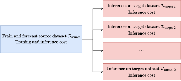
Figure 6: Flowchart of the zeros-shot forecasting regime on $D$ target datasets from one source datasets $(\mathcal{D}_{\text{source}})$. The blue square (left) represent the traditional setup of training a model and forecasting on such dataset. The red squares (red) represent the process of loading a pre-trained models and forecasting TS from a different TS dataset than the one used for training. In term of time, the time to train a model is almost always greater than the one from infering a target datasets.

We evaluated their performance in the zero-shot regime on all other datasets (M3, Tourism, Electricty, Traffic, Finance) by training models on the M4 dataset only using scaled TS as in [13]. The reason for this preprocessing step was to prevent catastrophic failure when the target dataset scale is different from that of the source dataset.

We tested 3 different setups for zero-shot forecasting, which we denote by $R_{O}$, $R_{SH,LT}$ and $R_{SH}$. $R_{O}$ is a setup where we use the same model to produce results on M4 (Table 1) and apply it on the target dataset. This required us to truncate the forecast or apply the model iteratively on the basis of previous forecasts to ensure the forecast size is the same as the target dataset. The model was not trained to operate when this condition occurs. $R_{SH}$ is a setup where the model is trained with the same number of iterations as $R_{O}$ but we specified the model’s forecast horizon to be the same that of the target datasets. $R_{SH,LT}$ is the same training regime as $R_{SH}$, but we allowed the model to consider TS samples from further in the past during training and trained the model with more iterations. The rationale of testing these training setup is to evaluate the impact of training the model longer for generalization and to to test the model in forecast condition it wasn’t trained to do (e.g. in $R_{O}$ when the forecast horizon of the target dataset exceed or is inferior to the forecast horizon of the target dataset).

When training the model, we consider an hyper-parameter $L_{H}$ which is a coefficient defining the length of training history immediately preceding the last point in the train part of the TS that is used to generate training sample. This coefficient multiplied by the forecast horizon determined the maximum number of most recent points in the train dataset for each TS to generate training sample. The higher that coeffcient, the further in the past we consider TS observation to train this model. To produce forecasts, we used the subset of the ensemble models trained on the same TS frequency to produce the multiple forecasts and combined them by median aggregation. Detailed explanations of this aggregation, selection of $L_{H}$ and the ensemble parameters used are given in B.

We compared against statistical baselines and other ML models such as DEEP-STATE [35], N-BEATS [39, 13], DEEP-AR [22], FFORMA [2], ES-RNN [42], Deep Factors [72] and many others including statistical baselines already evaluated on theses datasets. In reporting the accuracy of these models, we relied upon the accuracy and the pre-computed forecasts reported in their respective original paper.

M3, SMAPE Tourism, MAPE Electricity, ND Traffic, ND N-SHOT: Naive 16.59 SNaive 24.80 Naive 0.37 0.57 Comb [4] 13.52 ETS [61] 20.88 MatFact [54] 0.16 0.17 ForePro [52] 13.19 Theta [32] 20.88 DeepAR [22] 0.07 0.17 Theta [32] 13.01 ForePro [52] 19.84 DeepState [35] 0.08 0.17 DOTM [73] 12.90 Strato $\blacksquare$ 19.52 Theta [32] 0.08 0.18 EXP [74] 12.71 LCBaker [75] 19.35 ARIMA [30] 0.07 0.15 N-BEATS[39] 12.37 18.52 0.07 0.11 DEEP-AR*[22, 13] 12.67 19.27 0.09 0.19 ZERO-SHOT: ($R_{SH,LT}/R_{SH}/R_{O}$) M4 N-BEATS (G) scaled* [39] 12.36/12.67/12.72 18.90/20.16/24.14 0.09/0.09/0.08 0.16/0.16/0.14 M4 N-BEATS (I) scaled* [39] 12.43/12.63/12.66 19.43/20.58/23.26 0.10/0.09/0.08 0.16/0.16/0.14 M4 N-BEATS (g+i) scaled* [39] 12.38/12.61/12.64 19.04/20.22/23.43 0.10/0.09/0.08 0.16/0.16/0.14 M4 N-BEATS (P+G) scaled 12.48/12.65/12.65 18.99/19.98/22.85 0.09/0.09/0.08 0.16/0.18/0.14 M4 N-BEATS (P+I) scaled 12.69/12.76/12.72 20.54/20.97/23.18 0.09/0.10/0.09 0.17/0.17/0.16 M4 N-BEATS (P+G&I) scaled 12.56/12.67/12.64 19.50/20.24/22.79 0.09/0.09/0.08 0.16/0.16/0.14

Table 11: Averaged forecasting for the zero-shot regime for each dataset; lower values are better. Zero-shot forecasts are compared for N-BEATS and our approach. For the models in italic using the following references, we relied on their reported accuracy. For zero-shot results, we show the metrics for three training regimes: $R_{SH,LT}/R_{SH}/R_{O}$. $R_{O}$ is the same model used to produce the results on M4 (Table. 1), which required to truncation of the forecast or applying the model iteratively at the basis of previous forecasts to ensure the forecast size was the same that of the target dataset. $R_{SH}$ is trained in the same fashion as $R_{O}$ but we specified the model’s forecast horizon to be the same as that of the target datasets. $R_{SH,LT}$ is the same training regime as $R_{SH}$ except that the model is allowed to consider TS samples from further in the past while training: See Table. 10 for more detail. Results for models with * appended to their names are replicated from the original papers and $\blacksquare$ signifies an anonymous submission for which we do not know the methodology.

Daily $(H=14)N=(1^{\prime}222^{\prime}866)$ Weekly $(H=13,N=1^{\prime}091^{\prime}898)$ Monthly $(H=18,N=288^{\prime}114)$ Models OWA MDA Time (min.) OWA MDA Time (min.) OWA MDA Time (min.) N-SHOT: Naive 1.000 07.1 — 1.00 02.0 — 1.000 00.5 — ARIMA [30] 1.041 27.1 4685 1.059 28.9 3597 0.891 40.3 816 THETA [32] 0.995 49.4 241 0.993 53.5 262 0.913 61.4 49 SES [31] 1.000 09.3 174 1.001 05.2 160 1.000 02.9 25 HOLT [60] 1.081 49.6 167 1.116 53.9 160 0.931 60.3 42 ETS [61] 1.019 20.4 969 1.044 18.8 512 0.940 29.2 181 ZERO-SHOT: M4 N-BEATS (G) [39] 1.165 50.3 24 1.078 50.9 21 0.963 55.1 6 M4 N-BEATS (I) [39] 1.222 50.5 26 1.045 51.3 23 0.962 54.9 6 M4 N-BEATS (I+G) [39] 1.191 50.7 50 1.056 51.1 44 0.961 55.4 12 M4 N-BEATS (P+G) 1.210 48.5 25 1.098 51.6 21 0.973 54.4 6 M4 N-BEATS (P+I) 1.135 48.5 26 1.055 52.1 24 0.975 54.1 6 M4 N-BEATS (P+I&G) 1.139 49.0 51 1.044 52.0 45 0.973 54.4 12

Table 12: Comparison between statistical baselines and zero-shot application of the N-BEATS model in terms of OWA, MDA and time to produce forecast. Forecasts were made with the native zero-shot approach ($R_{O}$).

Table 11 describes the zero-shot performance of N-BEATS and N-BEATS(P). Several observations can be made:

1. N-BEATS(P) produces comparable zero-shot results to previous state-of-the-art models for all datasets. In other training regimes, where models trained with the same forecast horizon or longer ones, comparable levels of accuracy were observed.

2. Comparing with [13], where a different training regime was used, the difference between their results and ours highlights the importance of the optimization procedure to facilitate transfer to another dataset. In certain cases, some datasets (e.g., Tourism, will benefit from a longer training, to the detriment of the forecast accuracy on the source dataset. In other cases, like the Electricity dataset, no adjustments are required between the source and the target dataset.

3. The case of the Tourism dataset highlights the importance of ensuring that the forecast horizon of the source dataset used to train the model is longer than or equal of the target dataset; this is a key factor in producing reliable zero-shot forecasts.

Considering that the M4 dataset includes a large number of heterogenous TS that contain at least some TS with similar statistical properties to those present in the target dataset, zero-shot forecasting can be easily deployed with a pre-trained DNN model and can produce initial forecasts that are on par with the level of accuracy of multiple baselines, and sometimes benchmarks, very quickly at a minimal cost.

However, not all settings will benefit equally from this approach. The Finance dataset is a prime example of a setting where zero-shot forecasting produce mixed results. In this setting, the source TS dataset has very few TS to train from in comparison to the test sets. Also, these TS are very difficult to forecast in a univariate setting since they are almost all non-ergodic, heteroscedastic, and have high noise-to-signal ratio. Despite these added difficulties, both N-BEATS and N-BEATS(P) can produce forecasts at a comparable level to a single statistical model in term of MDA when using the $R_{O}$ training setup. However, the zero-shot regime achieved forecasts better than a naive one only by sampling these TS at a monthly frequency, which coincidentally is the largest pool of TS in M4 (48’000.) In comparison, the daily (3594) and weekly (227) subsets contain fewer TS. Hence, even under poor conditions of application for zero-shot N-BEATS(P), we can still produce preliminary forecasts quickly. These results highlight the importance of selecting a good source dataset but even in subpar conditions, our approach can still generalize well with respect to the MDA metric.

Appendix D Finance dataset: List of Securities Considered

Table 13: List of US traded funds used to create the finance dataset. The class columns correspond to the type of securities and the source columns specify where the TS was collected. See Tab. 14 for a brief description of the asset classes

Data Source: Yahoo
Ticker	Description	Class
DJAT	Dow Jones Asian Titan 50 Index	Regional Stock Index
DJI	Dow Jones Industrial Average	Stock Index (US)
DJT	Dow Jones Transportation Average	Stock Index (US)
DJU	Dow Jones Utility Average	Stock Index (US)
GSPC	S&P 500	Stock Index (US)
IXIC	NASDAQ Composite	Stock Index (US)
NDX	NASDAQ-100	Stock Index (US)
OEX	S&P 100	Stock Index (US)
XMI	NYSE Arca Major Market Index	Stock Index (US)
DX-Y.NYB	US Dollar/USDX - Index - Cash	Forex
FDCPX	Fidelity Select Computers	US Sector Stock Index
HSI	HANG SENG INDEX (Currency in HKD)	National Stock Index
Data Source: Fred
GOLDPMGBD228NLBM	Gold Fixing Price 3:00 P.M. (London time) in London Bullion Market & based in U.S. Dollars	Others
WILL4500IND	Wilshire 4500 Total Market Index	Stock Index (US)
WILL4500PR	Wilshire 4500 Price Index	Stock Index (US)
WILL5000IND	Wilshire 5000 Total Market Index	Stock Index (US)
WILL5000INDFC	Wilshire 5000 Total Market Full Cap Index	Stock Index (US)
WILL5000PR	Wilshire 5000 Price Index	Stock Index (US)
Data Source: FastTrack
FPX1	CAC 40 Ix	National Stock Index
SHCP	Shanghai Composite Ix	National Stock Index
SPXX	STOXX Europe 600 Ix	Regional Stock Index
SX5P	STOXX Europe 50 Ix	Regional Stock Index
A-CWI	MSCI ACWI DivAdj Idx	Global Stock Index
A-XUS	MSCI ACWI xUS DivAdj Idx	Global Stock Index
AUD-	US / Australia Foreign Exchange Rate	Forex
BBG-	CBOE US T-Bill 13-Week Yld Bd Ix	US Bonds - Gvmnt
BBG-9	BBG Barclay Agg Bond- US Universal TR Ix	US Bonds - Gvmnt
BBG-G	BBG Barclay Agg Bond- US Corp IG TR Ix	US Bonds - Gvmnt
BBG-H	ML US HY Bb-B Ix	US Bonds - Corp HY
BBG-I	BBG Barclay Agg Bond- US Agency Long Ix	US Bonds - Gvmnt
BBG-O	BBG Barclay Agg Bond- Yankee Ix	US Bonds - Gvmnt
BBG-S	BBG Barclay Agg Bond- US MBS Agncy TR Ix	US Bonds - Gvmnt
BBG-T	BBG Barclay Agg Bond- US MBS Agncy TR Ix	US Bonds - Gvmnt
BBG-U	BBG Muni Bond 3yr Idx	US Bonds - Gvmnt
BBG-Y	BBG Muni Bond 20yr Idx	US Bonds - Gvmnt
BBM-2	BBG Muni Bond 5yr Idx	US Bonds - Gvmnt
BBM-3	BofAML US Corp 5-7yr Total Return Ix	US Bonds - Corp Invst
BBM-5	BBG Muni Bond Composite Idx	US Bonds - Gvmnt
BBM-I	BBG Muni Bond Long Term Idx	US Bonds - Gvmnt
BBM-L	BBG Muni Bond 10yr Idx	US Bonds - Gvmnt
BBM-T	BBG Barclay Agg Bond- US Composite TR Ix	US Bonds - Gvmnt
CAD-	Canada / US Foreign Exchange Rate Ix	Forex
CDN-X	Canadian Dollar For 100 CDN Ix	Forex
CHF-	Switzerland/ US Foreign Exchange Rate Ix	Forex
CNY-	China / US Foreign Exchange Rate Ix	Forex
CR-TR	CRB Total Return Ix	Commodities
DBC	Invesco DB Commodity Index Tracking Fund	Commodities
DKK-	Denmark / US Foreign Exchange Rate Ix	Forex
DXY-Z	US Dollar Ix	Forex
EFA	iShares MSCI EAFE ETF	Regional Stock Index
EURO-	US/Euro Foreign Exchange Rate Ix	Forex
EWA	iShares ETF MSCI Australia	National Stock Index
EWC	iShares ETF MSCI Canada	National Stock Index
EWD	iShares ETF MSCI Sweden	National Stock Index
EWG	iShares ETF MSCI Germany	National Stock Index
EWH	iShares ETF MSCI Hong Kong	National Stock Index
EWI	iShares ETF MSCI Italy Capped	National Stock Index
EWJ	iShares MSCI Japan ETF	National Stock Index
EWK	iShares ETF MSCI Belgium Capped	National Stock Index
EWL	iShares ETF MSCI Switzerland Capped	National Stock Index
EWM	iShares ETF MSCI Malaysia	National Stock Index
EWN	iShares ETF MSCI Netherlands	National Stock Index
EWO	iShares ETF MSCI Austria Capped	National Stock Index
EWP	iShares ETF MSCI Spain Capped	National Stock Index
EWS	iShares ETF MSCI Singapore	National Stock Index
EWW	iShares ETF MSCI Mexico Capped	National Stock Index
EWY-X	MSCI Korea iShr Ix	National Stock Index
EWZ-X	MSCI Brazil iShr Ix	National Stock Index
FBIOX	Fidelity Select Biotechnology	US Sector Stock Index
FBMPX	Fidelity Select Communication Services Portfolio	US Sector Stock Index
FCYIX	Fidelity Select Industrials	US Sector Stock Index
FDAC-	Frankfurt Dax Ix	National Stock Index
FDFAX	Fidelity Select Consumer Staples	US Sector Stock Index
FDLSX	Fidelity Select Leisure	US Sector Stock Index
FEZ-X	Europe 50 STOXX stTr Ix	Regional Stock Index
FIDSX	Fidelity Select Financial Services	US Sector Stock Index
FNARX	Fidelity Select Natural Resources	US Sector Stock Index
FNMIX	Fidelity New Markets Income	Regional Stock Index
FRESX	Fidelity Fidelity Real Estate Investment Portfolio	Others
FSAGX	Fidelity Select Gold	US Sector Stock Index
FSAIX	Fidelity Select Air Transportation	US Sector Stock Index
FSAVX	Fidelity Select Automotive	US Sector Stock Index
FSCHX	Fidelity Select Chemicals	US Sector Stock Index
FSCPX	Fidelity Select Consumer Discretion	US Sector Stock Index
FSCSX	Fidelity Select software & Comp Service	US Sector Stock Index
FSDAX	Fidelity Select Defense & Aerospace	US Sector Stock Index
FSDCX	Fidelity Select Commun Equipment	US Sector Stock Index
FSDPX	Fidelity Select Materials	US Sector Stock Index
FSELX	Fidelity Select Semiconductors	US Sector Stock Index
FSENX	Fidelity Select Energy	US Sector Stock Index
FSESX	Fidelity Select Energy Service	US Sector Stock Index
FSHCX	Fidelity Select Health Care Service	US Sector Stock Index
FSHOX	Fidelity Select Const & Housing	US Sector Stock Index
FSLBX	Fidelity Select Brokrg & INV Mgt	US Sector Stock Index
FSLEX	Fidelity Select Environmental & Alt	US Sector Stock Index
FSNGX	Fidelity Select Natural Gas	US Sector Stock Index
FSPCX	Fidelity Select Insurance	US Sector Stock Index
FSPHX	Fidelity Select Health Care	US Sector Stock Index
FSPTX	Fidelity Select Technology	US Sector Stock Index
FSRBX	Fidelity Select Banking	US Sector Stock Index
FSRFX	Fidelity Select Transportation	US Sector Stock Index
FSRPX	Fidelity Select Retailing	US Sector Stock Index
FSTCX	Fidelity Select Telecommunications	US Sector Stock Index
FSUTX	Fidelity Select Utilities	US Sector Stock Index
FSVLX	Fidelity Select Consumer Finance	US Sector Stock Index
FTSE-	London FT-SE 100 Ix	National Stock Index
GBP-	US / UK Foreign Exchange Rate Ix	Forex
GLD	SPDR Gold Shares	Commodities
HKD-	Hong Kong / US Foreign Exchange Rate Ix	Forex
HY-	ML US HY Broadcastng Ix	US Bonds - Corp HY
HY-BC	ML US HY Build Mterl Ix	US Bonds - Corp HY
HY-BM	ML US HY Capitl Good Ix	US Bonds - Corp HY
HY-CG	ML US HY Chemicals Ix	US Bonds - Corp HY
HY-CH	ML US HY CCC & Lower Ix	US Bonds - Corp HY
HY-CL	ML US HY Containers Ix	US Bonds - Corp HY
HY-CN	ML US HY Consum Prod Ix	US Bonds - Corp HY
HY-CP	ML US HY Div Fin Svc Ix	US Bonds - Corp HY
HY-DF	ML US HY Div Media Ix	US Bonds - Corp HY
HY-DM	ML US HY Entert Film Ix	US Bonds - Corp HY
HY-EF	ML US HY Energy Ix	US Bonds - Corp HY
HY-EG	ML US HY Environmntl Ix	US Bonds - Corp HY
HY-EN	ML US HY Ex Telecom Ix	US Bonds - Corp HY
HY-ET	ML US HY Fd Bvrge Tb Ix	US Bonds - Corp HY
HY-FB	ML US HY Fd&Drg Retl Ix	US Bonds - Corp HY
HY-FD	ML US HY Homebldr Re Ix	US Bonds - Corp HY
HY-HB	ML US HY Healthcare Ix	US Bonds - Corp HY
HY-HC	ML US HY Insurance Ix	US Bonds - Corp HY
HY-IN	ML US HY Leisure Ix	US Bonds - Corp HY
HY-LE	ML US HY Metal Minng Ix	US Bonds - Corp HY
HY-MM	ML US HY Paper Ix	US Bonds - Corp HY
HY-PP	ML US HY Publsh Prnt Ix	US Bonds - Corp HY
HY-PR	ML US HY Restaurants Ix	US Bonds - Corp HY
HY-RS	ML US HY Super Retl Ix	US Bonds - Corp HY
HY-SR	ML US HY Steel Ix	US Bonds - Corp HY
HY-ST	ML US HY Services Ix	US Bonds - Corp HY
HY-SV	ML US HY Tech&Aerosp Ix	US Bonds - Corp HY
HY-TA	ML US HY Telecommnct Ix	US Bonds - Corp HY
HY-TC	ML US HY Cabl Sat Tv Ix	US Bonds - Corp HY
HY-TV	ML US HY Utilities Ix	US Bonds - Corp HY
HY-UT	ML US Indl Corps A Ix	US Bonds - Corp Invst
IC-1A	ML US Indl Corps AA Ix	US Bonds - Corp Invst
IC-2A	ML US Indl Corps AAA Ix	US Bonds - Corp Invst
IC-3A	ML US Indl Corps BBB Ix	US Bonds - Corp Invst
IEF	iShares ETF 7 10 Year Treasury Bond	US Bonds - Gvmnt
INE-X	MSCI Italy iShr Ix	National Stock Index
INH-X	MSCI Hong Kong iShr Ix	National Stock Index
INR-	India/ US Foreign Exchange Rate Ix	Forex
INR-X	MSCI Singapore iShr Ix	National Stock Index
IWC-X	Russell Microcap	Stock Index (US)
IXF-X	NASDAQ Financial-100	Stock Index (US)
JPY-	Japan/ US Foreign Exchange Rate Ix	Forex
KRW-	South Korea / US Exchange Rate Ix	Forex
LLQ-X	Russell Microcap - Dividend Adj	Stock Index (US)
LLR-X	Russell Microcap	Stock Index (US)
LQD	iShares iBoxx $ Investment Grade Corporate Bond ETF	US Bonds - Corp Invst
M-BRC	MSCI Emerging Markets BRIC DivAdj Idx	Global Stock Index
M-CN	MSCI China DivAdj Ix	National Stock Index
M-DEO	MSCI Dev Mkts Euro DivAdj Idx	Global Stock Index
M-WD	MSCI World DivAdj Idx	Global Stock Index
M16Y-	BofAML US Corporate A Effective Yield Ix	US Bonds - Corp Invst
M26Y-	BofAML US Corporate AA Effective Yield I	US Bonds - Corp Invst
M36Y-	BofAML US Corporate AAA Effective Yield	US Bonds - Corp Invst
M3EY-	BofAML US Corp AAA Option-Adj Spread Ix	US Bonds - Corp Invst
M46Y-	BofAML US Corporate BBB Effective Yield	US Bonds - Corp Invst
M56Y-	BofAML US Corporate 1-3 Year Effective Y	US Bonds - Corp Invst
M5EY-	BofAML US Corp 1-3Y Option-Adj Spread Ix	US Bonds - Corp Invst
M66Y-	BofAML US Corporate 3-5 Year Effective Y	US Bonds - Corp Invst
M6EY-	BofAML US Corp 3-5Y Option-Adj Spread Ix	US Bonds - Corp Invst
M76Y-	BofAML US Corporate 5-7 Year Effective Y	US Bonds - Corp Invst
M7TR-	BBG Muni Bond 7yr Idx	US Bonds - Gvmnt
M86Y-	BofAML US Corporate 7-10 Year Effective	US Bonds - Corp Invst
M8TR-	BBG Muni Bond 1yr Idx	US Bonds - Corp Invst
M96Y-	BofAML US Corporate 10-15 Year Effective	US Bonds - Corp Invst
M9EY-	BofAML US HY BB Option-Adj Spread Ix	US Bonds - Corp HY
MDY	StateSt ETF SPDR S&P MIDCAP 400	Stock Index (US)
MF6Y-	BofAML US Corporate 15 Year Effective Yi	US Bonds - Corp Invst
MFEY-	ML US T-Bill 0-3mo Div-Adj Ix	US Bonds - Gvmnt
ML-03	ML US T-Bill 1-10yrs Ix	US Bonds - Gvmnt
ML-10	ML US T-Bill 1-3yrs Div-Adj Ix	US Bonds - Gvmnt
ML-13	ML US T-Bill 12mo Div-Adj Ix	US Bonds - Gvmnt
ML-1Y	ML US T-Bill 3-5yrs Div-Adj Ix	US Bonds - Gvmnt
ML-35	ML US T-Bill 3-6mo Div-Adj Ix	US Bonds - Gvmnt
ML-36	ML US T-Bill 6mo Div-Adj Ix	US Bonds - Gvmnt
ML-6T	ML US T-Bill 7-10yrs Ix	US Bonds - Gvmnt
ML-70	BofAML US High Yield B Total Return Inde	US Bonds - Corp HY
ML-I0	ML US T-Bill 1-10yrs Infl-Lnk Ix	US Bonds - Gvmnt
ML-I1	BBG Barclay Agg Bond- TBill Tips TR Ix	US Bonds - Gvmnt
ML-TB	ML US Corp Non-Fd&Dru Ret Ix	US Bonds - Corp Invst
MLB-	BofAML US High Yield BB Total Return Ind	US Bonds - Corp HY
MLBB-	BofAML US High Yield CCC or Below Total	US Bonds - Corp HY
MLCC-	ML US HY Master II D-A H0A0 Ix	US Bonds - Corp HY
MLHY-	ML BBB Grade Div-Adj Muni Ix	US Bonds - Gvmnt
MLMB-	ML Municipal Master Div-Adj Ix	US Bonds - Gvmnt
MLMM-	ML US T-Bill Div-Adj Ix	US Bonds - Gvmnt
MXN-	Mexico / US Foreign Exchange Rate Ix	Forex
OSX-X	AMEX Oil Service HLDRS Ix	Commodities
PCY	Invesco Emerging Markets Sovereign Debt ETF & US Bonds - Corp HY
RTF-X	Russell Top 50	Stock Index (US)
RU2-D	Russell 2500 - Dividend Adj	Stock Index (US)
RUA-D	Russell 3000 - Dividend Adj	Stock Index (US)
RUA-X	Russell 3000	Stock Index (US)
RUI-D	Russell 1000 - Dividend Adj	Stock Index (US)
RUI-I	Russell 1000	Stock Index (US)
RUM-D	Russell MidCap - Dividend Adj	Stock Index (US)
RUP-D	Russell Top 200 - Dividend Adj	Stock Index (US)
RUP-X	Russell Top 200	Stock Index (US)
RUS-D	Russell Small Cap - Dividend Adj	Stock Index (US)
RUT-D	Russell 2000 - Dividend Adj	Stock Index (US)
RUT-U	Russell 2000 - Unadj	Stock Index (US)
S-100	S&P Global 100 Ix	Global Stock Index
SEK-	Sweden / US Foreign Exchange Rate Ix	Forex
SGD-	Singapore / US Foreign Exchange Rate Ix	Forex
SHY	iShares 1-3 Year Treasury Bond ETF	US Bonds - Gvmnt
THB-	Thailand / US Foreign Exchange Rate Ix	Forex
TIP	iShares TIPS Bond ETF	US Bonds - Gvmnt
TLT	iShares 20+ Year Treasury Bond ETF	US Bonds - Gvmnt
TWD-	Taiwan / US Foreign Exchange Rate Ix	Forex
UC-	ML US Corp 10 Yrs Ix	US Bonds - Corp Invst
UC-10	ML US Corp 15 Yrs Ix	US Bonds - Corp Invst
UC-15	ML US Corp Gs&Elct Utl 1-10 Yrs Ix	US Bonds - Corp Invst
UC-G1	ML US Corp Gas&Elect Utl Ix	US Bonds - Corp Invst
UC-G4	ML US Corp Phones 10-15 Yrs Ix	US Bonds - Corp Invst
UC-LC	ML US T-Bill 7-10yrs Infl-Lnk Ix	US Bonds - Gvmnt
UC-P1	ML US Corp Phones 15 Yrs Ix	US Bonds - Corp Invst
UC-P2	ML US Corp Utils&Phones Ix	US Bonds - Corp Invst
UC-UP	ML US Corp Large Cap Ix	US Bonds - Corp Invst
US05-	BofAML US Corporate 7-10yr Total Return	US Bonds - Corp Invst
UUP	Invesco DB US Dollar Index Bullish Fund	Forex
VASVX	Vanguard Selected Value Fund	Stock Index (US)
VBISX	Vanguard Short Term Bond Index	US Bonds - Gvmnt
VEIEX	Vanguard Emerging Market Stock Index INV	Regional Stock Index
VEXMX	Vanguard Extended Market Index Fund	Global Stock Index
VEXPX	Vanguard Explorer Fund INV	Stock Index (US)
VFICX	Vanguard Int. Term Investment Grade Bond Fund	US Bonds - Corp Invst
VFIIX	Vanguard GNMA INV	US Bonds - Gvmnt
VFISX	Vanguard Short-Term Treasury INV	US Bonds - Gvmnt
VFITX	Vanguard Intermediate Term Treasury Fund	US Bonds - Gvmnt
VFSTX	Vanguard Short-Term INV Growth Incm INV	US Bonds - Corp Invst
VGENX	Vanguard Energy INV	National Stock Index
VGHCX	Vanguard Health Care INV	National Stock Index
VGPMX	Vanguard Global Capital Cycles Fund	Stock Index (US)
VGSIX	Vanguard REIT Index INV	Others
VINEX	Vanguard International Explorer Fund	Global Stock Index
VNQ	Vanguard Real Estate Index Fund ETF Shares	Others
VTRIX	Vanguard International Value Fund	Global Stock Index
VTSMX	Vanguard Total Stock Markets Index INV	Global Stock Index
VUSTX	Vanguard Long-Term Treasury INV	US Bonds - Gvmnt
VWEHX	Vanguard Hi-Yield Corporate INV	US Bonds - Corp HY
VWESX	Vanguard Long-Term INV Growth Income INV	US Bonds - Corp Invst
VWIGX	Vanguard International Growth INV	Others
VWINX	Vanguard Wellesley Income INV	US Bonds - Gvmnt
VWO	Vanguard FTSE Emerging Markets Index Fund ETF Shares	Global Stock Index
VWUSX	Vanguard US Growth INV	Stock Index (US)
VXF	Vanguard Extended Market Index Fund ETF Shares	Global Stock Index
WDG-X	MSCI Germany iShr Ix	National Stock Index
WPB-X	MSCI Canada iShr Ix	National Stock Index
XLB	StateSt ETF Materials Select Sector SPDR	US Sector Stock Index
XLE	StateSt ETF Energy Select Sector SPDR Fd	US Sector Stock Index
XLF	StateSt ETF Financial Select Sector SPDR	US Sector Stock Index
XLI	StateSt ETF Industrial Sel Sector SPDR	US Sector Stock Index
XLK	StateSt ETF Tech Select Sector SPDR	US Sector Stock Index
XLP	StateSt ETF Consumer Staples SelSctrSPDR	US Sector Stock Index
XLU	StateSt ETF Utilities Select Sector SPDR	US Sector Stock Index
XLV	StateSt ETF Health Care Sel Sector SPDR	US Sector Stock Index
XLY	StateSt ETF Consumer DiscretnrySlSctSPDR	US Sector Stock Index
XLC	StateSt ETF Communication Service SlSctSPDR	US Sector Stock Index
XLRE	StateSt ETF Real Estate SlSctSPDR	US Sector Stock Index
VOX	Vanguard Communication Services Index Fund ETF Shares	US Sector Stock Index
IYR	iShares U.S. Real Estate ETF	US Sector Stock Index
XOI-I	AMEX Oil Ix	Commodities
ZAR-	South Africa/ US Exchange Rate Ix	Forex
NIKI	Tokyo Nikkei Ix	National Stock Index
BBM-1	BBG Muni Bond 1-10yr Blend Idx	US Bonds - Corp Invst
BBM-7	BBG Muni Bond 15yr Idx	US Bonds - Gvmnt
BBM-B	BBG Barclay Agg Bond- Lng Govt/Crd TR Ix	US Bonds - Corp Invst
BBM-F	US Treasury 5-Year Bd Yield Ix	US Bonds - Gvmnt
BRL-	Brazil / US Foreign Exchange Rate Ix	Forex
DIA	StateSt ETF SPDR Dow Jones IndustrilAvrg	Stock Index (US)
DJ-CO	DJ UBS Crude Oil Ix	Commodities
EWQ	iShares ETF MSCI France	National Stock Index
EWU	iShares ETF MSCI United Kingdom	National Stock Index
IC-3B	BofAML US Corporate A Semi-Annual Yield	US Bonds - Corp Invst
IEO-X	DJ US Oil & Gas iShr Ix	Commodities
M-CNA	MSCI China A DivAdj Ix	National Stock Index
M-DEA	MSCI EAFE DivAdj Idx	Global Stock Index
M-DEU	MSCI Dev Mkts EU DivAdj Idx	Regional Stock Index
M-DG7	MSCI Dev Mkts G7 Index DivAdj Idx	Global Stock Index
M-EM	MSCI Emerging Markets DivAdj Idx	Global Stock Index
M-EMA	MSCI Emerging Markets Asia DivAdj Idx	Regional Stock Index
M-EME	MSCI Emergin Martkets EMEA DivAdj Idx	Regional Stock Index
M-EMU	MSCI Emerging Markets Europe DivAdj Idx	Regional Stock Index
M1EY-	BofAML US Corporate AA Semi-Annual Yield	US Bonds - Corp Invst
M2EY-	BofAML US Corporate AAA Semi-Annual Yiel	US Bonds - Corp Invst
M3OA-	BofAML US Corporate BBB Semi-Annual Yiel	US Bonds - Corp Invst
M4EY-	BofAML US Corporate 1-3 Year Semi-Annual	US Bonds - Corp Invst
M5OA-	BofAML US Corporate 3-5 Year Semi-Annual	US Bonds - Corp Invst
M6OA-	BofAML US Corporate 5-7 Year Semi-Annual	US Bonds - Corp Invst
M7EY-	BofAML US Corporate 7-10 Year Semi-Annua	US Bonds - Corp Invst
M8EY-	BofAML US Corporate 10-15 Year Semi-Annu	US Bonds - Corp Invst
MBOA-	BofAML US Corporate 15 Year Semi-Annual	US Bonds - Corp Invst
QQQ	Nasdaq 100 ETF	Stock Index (US)
SP-GB	S&P Global BMI Idx DivAdj	Global Stock Index
SP-GL	S&P Global 1200 Idx DivAdj	Global Stock Index
SP-HB	S&P 500 High Beta Idx DivAdj	Global Stock Index
SP-IO	S&P Global 100 Idx DivAdj	Global Stock Index
SP-L4	S&P Latin America 40 Idx DivAdj	Regional Stock Index
SPY	StateSt ETF SPDR S&P 500	Stock Index (US)
ST-AG	Silver Spot	Commodities
ST-AU	Gold Spot	Commodities
ST-BC	Brent Crude Spot	Commodities
ST-CA	Cocoa Spot	Commodities
ST-CF	Coffee Bushel Spot	Commodities
ST-CO	Crude Oil Spot	Commodities
ST-CT	Cotton Bushel Spot	Commodities
ST-CU	Copper Spot	Commodities
ST-HO	Heating Oil Spot	Commodities
ST-NG	Natural Gas Spot	Commodities
ST-PD	Palladium Spot	Commodities
ST-PL	Platinum Spot	Commodities
WTI-B	Blmbrg WTI Crude Oil Sub Ix Total Return	Commodities
VIPSX	Vanguard Inflation-Protected Securities Fund Investor Shares	US Bonds - Gvmnt

TS type Description US Stock Index Index of US stocks, such as the S&P500 US Stock A fund (ETF or mutual funds) made up primarily of US stocks US Sector Stock Index US stock industry sector index Regional Stock Index Global region stock index, such as Europe National Stock Index Country stock index Global Stock Index Global / world stock index US Bonds - Gvmnt US treasury funds US Bonds - Corp Invst US corporate bond funds, investment grade US Bonds - Corp HY US bond funds, high yield Country Funds Country index fund Forex Foreign Exchange Commodities Commodities tracking fund Real Estate Real estate fund Other Other fund or index

Table 14: Brief description of the typea of TS used in the Finance dataset.

References

- [1] S. Makridakis, R. J. Hyndman, F. Petropoulos, Forecasting in social settings: The state of the art, International Journal of Forecasting 36 (1) (2020) 15–28.
- [2] P. Montero-Manso, G. Athanasopoulos, R. J. Hyndman, T. S. Talagala, Fforma: Feature-based forecast model averaging, International Journal of Forecasting 36 (1) (2020) 86–92.
- [3] S. Makridakis, E. Spiliotis, V. Assimakopoulos, The m5 accuracy competition: Results, findings and conclusions (10 2020).
- [4] S. Makridakis, E. Spiliotis, V. Assimakopoulos, The m4 competition: 100,000 time series and 61 forecasting methods, International Journal of Forecasting 36 (1) (2020) 54–74.
- [5] A.-A. Semenoglou, E. Spiliotis, S. Makridakis, V. Assimakopoulos, Investigating the accuracy of cross-learning time series forecasting methods, International Journal of Forecasting 37 (3) (2021) 1072–1084.
- [6] A. Choromanska, M. Henaff, M. Mathieu, G. B. Arous, Y. LeCun, The loss surfaces of multilayer networks, in: Artificial intelligence and statistics, PMLR, 2015, pp. 192–204.
- [7] P. Nakkiran, G. Kaplun, Y. Bansal, T. Yang, B. Barak, I. Sutskever, Deep double descent: Where bigger models and more data hurt, arXiv preprint arXiv:1912.02292 (2019).
- [8] Y. Dauphin, R. Pascanu, C. Gulcehre, K. Cho, S. Ganguli, Y. Bengio, Identifying and attacking the saddle point problem in high-dimensional non-convex optimization, arXiv preprint arXiv:1406.2572 (2014).
- [9] F. Bach, Breaking the curse of dimensionality with convex neural networks, The Journal of Machine Learning Research 18 (1) (2017) 629–681.
- [10] Z. Chen, Y. Cao, Y. Liu, H. Wang, T. Xie, X. Liu, A comprehensive study on challenges in deploying deep learning based software, in: Proceedings of the 28th ACM Joint Meeting on European Software Engineering Conference and Symposium on the Foundations of Software Engineering, 2020, pp. 750–762.
- [11] A. Paleyes, R.-G. Urma, N. D. Lawrence, Challenges in deploying machine learning: a survey of case studies, arXiv preprint arXiv:2011.09926 (2020).
- [12] T. Januschowski, Forecasting at amazon: Problems, methods and systems, https://forecasters.org/wp-content/uploads/gravity_forms/7-c6dd08fee7f0065037affb5b74fec20a/2017/07/Januschowski_Tim_ISF2017.pdf, accessed: 2021–06-15 (2018).
- [13] B. N. Oreshkin, D. Carpov, N. Chapados, Y. Bengio, Meta-learning framework with applications to zero-shot time-series forecasting, arXiv preprint arXiv:2002.02887 (2020).
- [14] A. Hooshmand, R. Sharma, Energy predictive models with limited data using transfer learning, in: Proceedings of the Tenth ACM International Conference on Future Energy Systems, 2019, pp. 12–16.
- [15] P. Gupta, P. Malhotra, J. Narwariya, L. Vig, G. Shroff, Transfer learning for clinical time series analysis using deep neural networks, Journal of Healthcare Informatics Research 4 (2) (2020) 112–137.
- [16] P. Montero-Manso, R. J. Hyndman, Principles and algorithms for forecasting groups of time series: Locality and globality, International Journal of Forecasting (2021).
- [17] S. Makridakis, E. Spiliotis, V. Assimakopoulos, The m4 competition: Results, findings, conclusion and way forward, International Journal of Forecasting 34 (4) (2018) 802–808.
- [18] Google, 2017. web traffic time series forecasting., https://www.kaggle.com/c/web-traffic-time-series-forecasting, accessed: 2021–06-15 (2017).
- [19] Y. Rubanova, T. Q. Chen, D. K. Duvenaud, Latent ordinary differential equations for irregularly-sampled time series, in: Advances in Neural Information Processing Systems, 2019, pp. 5321–5331.
- [20] S. Smyl, J. Ranganathan, A. Pasqua, M4 forecasting competition: Introducing a new hybrid es-rnn model, URL: https://eng. uber. com/m4-forecasting-competition (2018).
- [21] V. Ekambaram, K. Manglik, S. Mukherjee, S. S. K. Sajja, S. Dwivedi, V. Raykar, Attention based multi-modal new product sales time-series forecasting, in: Proceedings of the 26th ACM SIGKDD International Conference on Knowledge Discovery & Data Mining, 2020, pp. 3110–3118.
- [22] D. Salinas, V. Flunkert, J. Gasthaus, T. Januschowski, Deepar: Probabilistic forecasting with autoregressive recurrent networks, International Journal of Forecasting 36 (3) (2020) 1181–1191.
- [23] J.-H. Böse, V. Flunkert, J. Gasthaus, T. Januschowski, D. Lange, D. Salinas, S. Schelter, M. Seeger, Y. Wang, Probabilistic demand forecasting at scale, Proceedings of the VLDB Endowment 10 (12) (2017) 1694–1705.
-
[24]
C. Liang, Y. Lu,
Using
automl for time series forecasting (2020).
URL https://ai.googleblog.com/2020/12/using-automl-for-time-series-forecasting.html - [25] F. Bell, S. Smyl, Forecasting at uber: An introduction, Uber Engineering (2018).
-
[26]
N. Laptev,
Time-series
modeling with neural networks at uber (2020).
URL https://forecasters.org/wp-content/uploads/gravity_forms/7-c6dd08fee7f0065037affb5b74fec20a/2017/07/Laptev_Nikolay_ISF2017.pdf -
[27]
B. Banushev, R. Barclay,
Enhancing
trading strategies through cloud services and machine learning (Jan 2021).
URL https://aws.amazon.com/fr/blogs/industries/enhancing-trading-strategies-through-cloud-services-and-machine-learning/ - [28] J. H. Cochrane, Asset pricing: Revised edition, Princeton university press, 2009.
- [29] P. Chatigny, R. Goyenko, C. Zhang, Asset pricing with attention guided deep learning, Available at SSRN (2021).
- [30] G. E. Box, G. M. Jenkins, G. C. Reinsel, G. M. Ljung, Time series analysis: forecasting and control, John Wiley & Sons, 2015.
- [31] R. Hyndman, A. B. Koehler, J. K. Ord, R. D. Snyder, Forecasting with exponential smoothing: the state space approach, Springer Science & Business Media, 2008.
- [32] V. Assimakopoulos, K. Nikolopoulos, The theta model: a decomposition approach to forecasting, International journal of forecasting 16 (4) (2000) 521–530.
- [33] J. D. Hamilton, A new approach to the economic analysis of nonstationary time series and the business cycle, Econometrica: Journal of the Econometric Society (1989) 357–384.
- [34] R. Prado, G. Huerta, M. West, Bayesian time-varying autoregressions: Theory, methods and applications, Resenhas do Instituto de Matemática e Estatística da Universidade de São Paulo 4 (4) (2000) 405–422.
- [35] S. S. Rangapuram, M. W. Seeger, J. Gasthaus, L. Stella, Y. Wang, T. Januschowski, Deep state space models for time series forecasting, in: Advances in NIPS, 2018, pp. 7785–7794.
- [36] S. Li, X. Jin, Y. Xuan, X. Zhou, W. Chen, Y.-X. Wang, X. Yan, Enhancing the locality and breaking the memory bottleneck of transformer on time series forecasting, in: Advances in Neural Information Processing Systems, 2019, pp. 5243–5253.
- [37] N. Wu, B. Green, X. Ben, S. O’Banion, Deep transformer models for time series forecasting: The influenza prevalence case, arXiv preprint arXiv:2001.08317 (2020).
- [38] S. Makridakis, E. Spiliotis, V. Assimakopoulos, Statistical and machine learning forecasting methods: Concerns and ways forward, PloS one 13 (3) (2018) e0194889.
- [39] B. N. Oreshkin, D. Carpov, N. Chapados, Y. Bengio, N-beats: Neural basis expansion analysis for interpretable time series forecasting, in: International Conference on Learning Representations, 2019.
- [40] R. T. Clemen, Combining forecasts: A review and annotated bibliography, International journal of forecasting 5 (4) (1989) 559–583.
- [41] A. Timmermann, Forecast combinations, Handbook of economic forecasting 1 (2006) 135–196.
- [42] S. Smyl, A hybrid method of exponential smoothing and recurrent neural networks for time series forecasting, International Journal of Forecasting 36 (1) (2020) 75–85.
- [43] R. B. Cleveland, W. S. Cleveland, J. E. McRae, I. Terpenning, Stl: a seasonal-trend decomposition, Journal of official statistics 6 (1) (1990) 3–73.
- [44] L. Breiman, Bagging predictors, Machine learning 24 (2) (1996) 123–140.
- [45] I. Žliobaitė, Learning under concept drift: an overview, arXiv preprint arXiv:1010.4784 (2010).
- [46] Z.-H. Zhou, Ensemble methods: foundations and algorithms, CRC press, 2012.
- [47] V. Nair, G. E. Hinton, Rectified linear units improve restricted boltzmann machines, in: Icml, 2010.
- [48] U. C. Bureau, X-13arima-seats reference manual (2016).
-
[49]
D. P. Kingma, J. Ba, Adam: A method for
stochastic optimization, in: Y. Bengio, Y. LeCun (Eds.), 3rd International
Conference on Learning Representations, ICLR 2015, San Diego, CA, USA, May
7-9, 2015, Conference Track Proceedings, 2015.
URL http://arxiv.org/abs/1412.6980 - [50] A. J. Koning, P. H. Franses, M. Hibon, H. O. Stekler, The m3 competition: Statistical tests of the results, International Journal of Forecasting 21 (3) (2005) 397–409.
- [51] G. Athanasopoulos, R. J. Hyndman, H. Song, D. C. Wu, The tourism forecasting competition, International Journal of Forecasting 27 (3) (2011) 822–844.
- [52] G. Athanasopoulos, R. J. Hyndman, The value of feedback in forecasting competitions, International Journal of Forecasting 27 (3) (2011) 845–849.
-
[53]
D. Dua, C. Graff, UCI machine learning
repository (2017).
URL http://archive.ics.uci.edu/ml - [54] H.-F. Yu, N. Rao, I. S. Dhillon, Temporal regularized matrix factorization for high-dimensional time series prediction, in: Advances in neural information processing systems, 2016, pp. 847–855.
- [55] P. Chatigny, J.-M. Patenaude, S. Wang, Spatiotemporal adaptive neural network for long-term forecasting of financial time series, International Journal of Approximate Reasoning 132 (2021) 70–85.
- [56] R. J. Hyndman, Y. Khandakar, et al., Automatic time series forecasting: the forecast package for r, Journal of statistical software 27 (3) (2008) 1–22.
- [57] R. J. Hyndman, A. B. Koehler, Another look at measures of forecast accuracy, International journal of forecasting 22 (4) (2006) 679–688.
- [58] L. Van der Maaten, G. Hinton, Visualizing data using t-sne., Journal of machine learning research 9 (11) (2008).
- [59] R. Hyndman, Y. Kang, P. Montero-Manso, T. Talagala, E. Wang, Y. Yang, M. O’Hara-Wild, tsfeatures: Time series feature extraction, R package version 1 (0) (2019).
- [60] C. Chatfield, M. Yar, Prediction intervals for multiplicative holt-winters, International Journal of Forecasting 7 (1) (1991) 31–37.
- [61] R. J. Hyndman, A. B. Koehler, R. D. Snyder, S. Grose, A state space framework for automatic forecasting using exponential smoothing methods, International Journal of forecasting 18 (3) (2002) 439–454.
- [62] I. Goodfellow, Y. Bengio, A. Courville, Y. Bengio, Deep learning, Vol. 1, MIT press Cambridge, 2016.
- [63] M. Pawlikowski, A. Chorowska, Weighted ensemble of statistical models, International Journal of Forecasting 36 (1) (2020) 93–97.
- [64] P. Agathangelou, D. Trihinas, I. Katakis, Correlation analysis of forecasting methods: The case of the m4 competition, International Journal of Forecasting 36 (1) (2020) 212–216.
- [65] R. F. Engle, Autoregressive conditional heteroscedasticity with estimates of the variance of united kingdom inflation, Econometrica: Journal of the econometric society (1982) 987–1007.
- [66] T. Teräsvirta, Specification, estimation, and evaluation of smooth transition autoregressive models, Journal of the american Statistical association 89 (425) (1994) 208–218.
- [67] P. C. Phillips, P. Perron, Testing for a unit root in time series regression, Biometrika 75 (2) (1988) 335–346.
- [68] D. Kwiatkowski, P. C. Phillips, P. Schmidt, Y. Shin, et al., Testing the null hypothesis of stationarity against the alternative of a unit root, Journal of econometrics 54 (1-3) (1992) 159–178.
- [69] L. v. d. Maaten, G. Hinton, Visualizing data using t-sne, Journal of machine learning research 9 (Nov) (2008) 2579–2605.
- [70] A. Asuncion, D. Newman, Uci machine learning repository (2007).
- [71] L. Vincent, N. Thome, Shape and time distortion loss for training deep time series forecasting models, in: Advances in NIPS, 2019, pp. 4191–4203.
- [72] Y. Wang, A. Smola, D. C. Maddix, J. Gasthaus, D. Foster, T. Januschowski, Deep factors for forecasting, arXiv preprint arXiv:1905.12417 (2019).
- [73] J. A. Fiorucci, T. R. Pellegrini, F. Louzada, F. Petropoulos, A. B. Koehler, Models for optimising the theta method and their relationship to state space models, International Journal of Forecasting 32 (4) (2016) 1151–1161.
- [74] E. Spiliotis, V. Assimakopoulos, K. Nikolopoulos, Forecasting with a hybrid method utilizing data smoothing, a variation of the theta method and shrinkage of seasonal factors, International Journal of Production Economics 209 (2019) 92–102.
- [75] L. C. Baker, J. Howard, Winning methods for forecasting tourism time series, International Journal of Forecasting 27 (3) (2011) 850–852.