Can We Leverage Predictive Uncertainty to Detect Dataset Shift and Adversarial Examples in Android Malware Detection?

Abstract.

The deep learning approach to detecting malicious software (malware) is promising but has yet to tackle the problem of dataset shift, namely that the joint distribution of examples and their labels associated with the test set is different from that of the training set. This problem causes the degradation of deep learning models without users’ notice. In order to alleviate the problem, one approach is to let a classifier not only predict the label on a given example but also present its uncertainty (or confidence) on the predicted label, whereby a defender can decide whether to use the predicted label or not. While intuitive and clearly important, the capabilities and limitations of this approach have not been well understood. In this paper, we conduct an empirical study to evaluate the quality of predictive uncertainties of malware detectors. Specifically, we re-design and build 24 Android malware detectors (by transforming four off-the-shelf detectors with six calibration methods) and quantify their uncertainties with nine metrics, including three metrics dealing with data imbalance. Our main findings are: (i) predictive uncertainty indeed helps achieve reliable malware detection in the presence of dataset shift, but cannot cope with adversarial evasion attacks; (ii) approximate Bayesian methods are promising to calibrate and generalize malware detectors to deal with dataset shift, but cannot cope with adversarial evasion attacks; (iii) adversarial evasion attacks can render calibration methods useless, and it is an open problem to quantify the uncertainty associated with the predicted labels of adversarial examples (i.e., it is not effective to use predictive uncertainty to detect adversarial examples).

1. Introduction

Malware is a big threat to cybersecurity. Despite tremendous efforts, communities still suffer from this problem because the number of malware examples consistently increases. For example, Kaspersky (Lab, 2020) detected 21.6 million unique malware in 2018, 24.6 million in 2019, and 33.4 million in 2020. This highlights the necessity of automating malware detection via machine learning techniques (Ye et al., 2017). However, a fundamental assumption made by machine learning is that the training data distribution and the test data distribution are identical. In practice, this assumption is often invalid because of the dataset shift problem (Quionero-Candela et al., 2009). Note that dataset shift is related to, but different from, the concept drift problem, which emphasizes that the conditional distribution of the labels conditioned on the input associated with the test data is different from its counterpart associated with the training data (Widmer and Kubat, 1996). While some people use these two terms interchangeably (Žliobaitė et al., 2016; Lu et al., 2019), we choose to use dataset shift because it is a broader concept than concept drift.

Several approaches have been proposed for alleviating the dataset shift problem, such as: periodically retraining malware detectors (Xu et al., 2014; Chen et al., 2017), extracting invariant features (Zhang et al., 2020), and detecting example anomalies (Jordaney et al., 2017). One fundamental open problem is to quantify the uncertainty that is inherent to the outcomes of malware detectors (or the confidence a detector has in its prediction). A well-calibrated uncertainty indicates the potential risk of the accuracy decrease and enables malware analysts to conduct informative decisions (i.e., using the predicted label or not). One may argue that a deep learning model associates its label space with a probability distribution. However, this “as is” method is poorly calibrated and causes poor uncertainty estimates (Guo et al., 2017). This problem has motivated researchers to propose multiple methods to calibrate the probabilities, such as: variational Bayesian inference (Blundell et al., 2015), Monte Carlo dropout (Gal and Ghahramani, 2016), stochastic gradient MCMC (Welling and Teh, 2011), and non-Bayesian methods such as ensemble (Lakshminarayanan et al., 2017). Quantifying the uncertainty associated with predicted labels (i.e., predictive uncertainty) in the presence of dataset shift has received a due amount of attention in the context of image classification (Blundell et al., 2015; Lakshminarayanan et al., 2017), medical diagnoses (Leibig et al., 2017), and natural language processing (Snoek et al., 2019), but not in the context of malware detection. This motivates us to answer the question in the title.

Our contributions. In this paper, we empirically quantify the predictive uncertainty of 24 deep learning-based Android malware detectors. These detectors correspond to combinations of four malware detectors, which include two multiple layer perceptron based methods (i.e., DeepDrebin (Grosse et al., 2017) and MultimodalNN (Kim et al., 2019)) and one convolutional neural network based method (DeepDroid (McLaughlin et al., 2017)), and the recurrent neural network based method (Droidetec (Ma et al., 2020)); and six calibration methods, which are vanilla (no effort made for calibration), temperature scaling (Guo et al., 2017), Monte Carlo (MC) dropout (Gal and Ghahramani, 2016), Variational Bayesian Inference (VBI) (Snoek et al., 2019), deep ensemble (Lakshminarayanan et al., 2017) and its weighted version. The vanilla and temperature scaling calibration methods belong to the post-hoc strategy, while the others are ad-hoc and require us to transform the layers of an original neural network in a principled manner (e.g., sampling parameters from a learned distribution). In order to evaluate the quality of predictive uncertainty on imbalanced datasets, we propose useful variants of three standard metrics.

By applying the aforementioned 24 malware detectors to three Android malware datasets, we draw the following insights: (i) We can leverage predictive uncertainty to achieve reliable malware detection in the presence of dataset shift to some extent, while noting that a defender should trust the predicted labels with uncertainty below a certain threshold. (ii) Approximate Bayesian methods are promising to calibrate and generalize malware detectors to deal with dataset shift. (iii) Adversarial evasion attacks can render calibration methods useless and thus the predictive uncertainty.

We have made the code of our framework publicly available at https://github.com/deqangss/malware-uncertainty. It is worth mentioning that after the present paper is accepted, we became aware of a preprint (Nguyen et al., 2021), which investigates how to leverage predictive uncertainty to deal with false positives of Windows malware detectors, rather than dealing with dataset shift issues.

2. Problem Statement

2.1. Android Apps and Malware Detection

Since Android malware is a major problem and deep learning is a promising technique, our empirical study focuses on Android malware detection. Recall that an Android Package Kit (APK) is a zipped file that mainly contains: (i) AndroidManifest.xml, which declares various kinds of attributes about the APK (e.g., package name, required permissions, activities, services, hardware); (ii) classes.dex, which contains the APK’s functionalities that can be understood by the Java virtual machines (e.g., Android Runtime); (iii) res folder and resources.arsc, which contain the resources used by an APK; (iv) lib folder, which contains the native binaries compatible to different Central Processing Unit (CPU) architectures (e.g., ARM and x86); (v) META-INF folder, which contains the signatures of an APK. For analysis purposes, one can unzip an APK to obtain its files in the binary format, or disassemble an APK by using an appropriate tool (e.g., Apktool (Tumbleson and Wiśniewski, 2020) and Androguard (Desnos, 2020)), to obtain human-readable codes and manifest data (e.g., AndroidManifest.xml).

A malware detector is often modeled as a supervised binary classifier that labels an example as benign (‘0’) or malicious (‘1’). Let $\mathcal{Z}$ denote the example space (i.e., consisting of benign and malicious software) and $\mathcal{Y}=\{0,1\}$ denote the label space. Let $p^{\ast}(z,y)=p^{\ast}(y|z)p^{\ast}(z)$ denote the underlying joint distribution, where $z\in\mathcal{Z}$ and $y\in\mathcal{Y}$. The task of malware detection deals with the conditional distribution $p^{\ast}(y|z)$. Specifically, given a software sample $z\in\mathcal{Z}$, we consider Deep Neural Network (DNN) $p(y=1|z,\theta)$, which uses the sigmoid function in its output layer, to model $p^{\ast}(y|z)$, where $\theta$ represents the learnable parameters. A detector denoted by $f:\mathcal{Z}\to\mathcal{Y}$, which consists of DNNs and is learned from the training set $D_{train}$, returns 1 if $p(y=1|z,\theta)\geq 0.5$ and 0 otherwise. We obtain $p(y=0|z)=1-p(y=1|z,\theta)$. Moreover, let $p^{\prime}(z,y)$ denote the underlying distribution of test dataset $D_{test}$.

2.2. Problem Statement

There are two kinds of uncertainty associated with machine learning: epistemic vs. aleatoric (Snoek et al., 2019). The epistemic uncertainty tells us about which region of the input space is not perceived by a model (Bhatt et al., 2020). That is, a data sample in the dense region will get a low epistemic uncertainty and get a high epistemic uncertainty in the sparse region. On the other hand, the aleatoric uncertainty is triggered by data noises and is not investigated in this paper.

It is widely assumed that $p^{\prime}(z,y)=p^{*}(z,y)$ in malware detection and in the broader context of machine learning. However, this assumption does not hold in the presence of dataset shift, which reflects non-stationary environments (e.g., data distribution changed over time or the presence of adversarial evasion attacks) (Quionero-Candela et al., 2009). Most dataset shifts possibly incur changes in terms of epistemic uncertainty (excluding label flipping or concept of input $z$ changed thoroughly). We consider three settings that potentially trigger the $p^{\prime}(z,y)\neq p^{\ast}(z,y)$:

• Out of source: The $D_{test}$ and $D_{train}$ are drawn from different sources (Demontis et al., 2017).

• Temporal covariate shift: The test data or $p^{\prime}(z)$ evolves over time (Pendlebury et al., 2019).

• Adversarial evasion attack: The test data is manipulated adversarially; i.e., $(z^{\prime},y=1)\sim p^{\prime}(z,y=1)$ is perturbed from $(z,y=1)\sim p^{\ast}(z,y=1)$, where $z^{\prime}$ and $z$ have the same functionality and ‘$\sim$’ denotes “is sampled from” (Li and Li, 2020).

One approach to coping with these kinds of dataset shifts is to make a malware detector additionally quantify the uncertainty associated with a prediction so that a decision-maker decides whether to use the prediction (Lakshminarayanan et al., 2017; Snoek et al., 2019; Wang et al., 2021). This means that a detector $p(y|z,\theta)$ should be able to model $p^{\ast}(y|z)$ well while predicting examples $z$ of $(z,y)\sim p^{\prime}(z,y)$ with high uncertainties when $(z,y)\not\sim p^{\ast}(z,y)$, where $\not\sim$ denotes “does not obey the distribution of”. Specifically, the quality of prediction uncertainty can be assessed by their confidence scores. This can be achieved by leveraging the notion of calibration (Lakshminarayanan et al., 2017). A malware detector is said to be well-calibrated if the detector returns a same confidence score $q\in[0,1]$ for a set of test examples $Z_{q}\subseteq\mathcal{Z}$, in which the malware examples are distributed as $q$ (Vaicenavicius et al., 2019). Formally, let $\Pr(y=1|Z_{q})$ denote the proportion of malware examples in the set $Z_{q}$ that are indeed malicious. We have

Definition 0 (Well-calibrated malware detector, adapted from (Vaicenavicius et al., 2019)).

A probabilistic malware detector $p(\cdot,\theta):\mathcal{Z}\to[0,1]$ is well-calibrated if for each confidence $q\in[0,1]$ and $Z_{q}=\{z:p(y=1|z,\theta)=q,\forall z\in\mathcal{Z}\}$, it holds that $\Pr(y=1|Z_{q})=q$.

Note that Definition 2.1 means that for a well-calibrated detector, the fraction of malware examples in example set $Z_{q}$ is indeed $q$. This means that we can use $q$ as a confidence score for quantifying uncertainty when assessing the trustworthiness of a detector’s predictions. This also implies that detection accuracy and well-calibration are two different concepts. This is so because an accurate detector is not necessarily well-calibrated (e.g., when correct predictions with confidence scores near 0.5). Moreover, a well-calibrated malware detector is also not necessarily accurate.

It would be ideal if we can rigorously quantify or prove the uncertainty (or bounds) associated with a malware detector. However, this turns out to be a big challenge that has yet to be tackled. This motivates us to conduct an empirical study to characterize the uncertainty associated with Android malware detectors. Hopefully the empirical findings will contribute to theoretical breakthrough in the near future.

Specifically, our empirical study is centered at the question in title, which is further disintegrated as four Research Questions (RQs) as follows:

• RQ1: What is the predictive uncertainty of malware detectors in the absence of dataset shift?

• RQ2: What is the predictive uncertainty of malware detectors with respect to out-of-source examples?

• RQ3: What is the predictive uncertainty of malware detectors under temporal covariate shift?

• RQ4: What is the predictive uncertainty of malware detectors under adversarial evasion attacks?

Towards answering these questions, we need to empirically study the predictive distribution $p(y|z,\theta)$ of malware detectors in a number of scenarios.

3. Empirical Analysis Methodology

In order to design a competent methodology, we need to select malware detector that are accurate in detecting malware, select the calibration methods that are appropriate for these detectors, and metrics. This is important because a “blindly” designed methodology would suffer from incompatibility issues (e.g., integrating different feature extractions modularly, or integrating post- and ad-hoc calibration methods together). The methodology will be designed in a modular way so that it can be extended to accommodate other models or calibration methods in a plug-and-play fashion.

3.1. Selecting Candidate Detectors

We focus on deep learning based Android malware detectors and more specifically choose the following four Android malware detectors.

DeepDrebin (Grosse et al., 2017): It is a Multiple Layer Perceptron (MLP)-based malware detector learned from the Drebin features (Arp et al., 2014), which are extracted from the AndroidManifest.xml file and the classes.dex file reviewed above. These features are represented by binary vectors, with each element indicating the presence or absence of a feature.

MultimodalNN (Kim et al., 2019): It is a multimodal detector that contains five headers and an integrated part, all of which are realized by MLP. The 5 headers respectively learn from 5 kinds of features: (i) permission-component-environment features extracted from the manifest file; (ii) strings (e.g., IP address); (iii) system APIs; (iv) Dalvik opcode; and (v) ARM opcodes from native binaries. These features are represented by their occurrence frequencies. These 5 headers produce 5 pieces of high-level representations, which are concatenated to pass through the integrated part for classification.

DeepDroid (McLaughlin et al., 2017): It is Convolutional Neural Network (CNN)-based and uses the TextCNN architecture (Kim, 2014). The features are Dalvik opcode sequences of smali codes.

Droidetec (Ma et al., 2020) is an RNN-based malware detector with the architecture of Bi-directional Long Short Term Memory (Bi-LSTM) (Thireou and Reczko, 2007). Droidetec partitions a Function Call Graph (FCG) into sequences according to the caller-callee relation and then concatenates these sequences for passing through the Bi-LSTM model.

These detectors leverage several types of deep learning models. Indeed, we also implement an end-to-end method (R2-D2 (Huang and Kao, 2018)) and find it ineffectiveness due to the over-fitting issue. Therefore, we eliminate it from our study.

3.2. Selecting Calibration Methods

In order to select calibration methods to calibrate the malware detectors, the following two criteria can be used: (i) they are known to be effective and (ii) they are scalable for learning a deep learning model. In particular, the preceding highlights the importance of the computational complexity of a calibration method. Based on a previous study (Snoek et al., 2019), these criteria lead us to select the following six methods.

Vanilla: It serves as a baseline and means that no effort is made to calibrate a model $p(y=1|z,\theta)$.

Temperature scaling (Temp scaling) (Guo et al., 2017): It is a post-processing method that learns extra parameters to scale the logits of deep learning models on the validation set, where logits are the input of the activation of $\operatorname{sigmoid}$.

Monte Carlo dropout (MC dropout) (Gal and Ghahramani, 2016): It technically adds a dropout layer (Srivastava et al., 2014) before the input of every layer contained in a model. This dropout operation is performed in both the training and test phases different from the normal usage that turns dropout on in the training phase and off in the test phase. In theory, MC dropout is an approximate Bayesian inference, which takes as input an example $z$ and marginalizes the parameters $\theta$ out for returning the predictive probability:

(1) $$p(y=1|z,D_{train})=\int~{} p(y=1|z,\theta)p(\theta|D_{train})d\theta$$

Due to the intricate neural networks, an analytical solution to obtaining $p(\theta|D_{train})$ is absent. One alternative is to approximate $p(\theta|D_{train})$ via a known functional form distribution $q(\omega)$ with variables $\omega$, leading to $p(y|z,D_{train})\approx\mathbb{E}_{q(\theta|\omega)}p(y|z,\theta)$. Specifically, let $\theta=\{\mathbf{W}_{i}\}_{i=1}^{l}$ be the set of $l$ parameters of a neural network, MC dropout defines $q(\omega)$ as:

(2) $$\mathbf{W}_{i}=\mathbf{M}_{i}\cdot\mathbf{V}_{i}~{}~{}\text{with}~{}~{}\mathbf{V}_{i}\sim\operatorname{Bernoulli}(r_{i}),$$

where $\mathbf{M}_{i}$ is learnable variables, entities of $\mathbf{V}_{i}$ are sampled from a Bernoulli distribution with the probability $r_{i}$ (i.e., dropout rate), and $\omega=\{\mathbf{M}_{i},r_{i}\}_{i=1}^{l}$. In the training phase, variational learning is leveraged to look for $\{\mathbf{M}_{i}\}_{i=1}^{l}$ (Graves, 2011; Blundell et al., 2015), which minimizes the Kullback-Leibler (KL) divergence between $p(\theta|D_{train})$ and $q(\omega)$. In the test phase, Eq.(1) is degraded by averaging $T(T>0)$ models $\{\theta^{j}\}_{j=1}^{T}$ (each of which is sampled from $q(\omega)$), namely:

(3) $$p(y=1|z)=\frac{1}{T}\sum_{j=1}^{T}~{}p(y=1|z,\theta^{i}).$$

Eq.3 says $p(y=1|z)$ is obtained just by keeping the dropout switched and averaging the results of $T$ times predictions.

Variational Bayesian Inference (VBI) (Snoek et al., 2019): It is also an approximate Bayesian method. Distinguishing from MC dropout, the parameters $\theta$ of neural network are directly sampled from a known form distribution $q(\omega)$ with variables $\omega$. That is

(4) $$\mathbf{W}\sim q(\omega)~{}~{}\text{with}~{}~{}\mathbf{W}\in\theta$$

The training and test manner is the same as MC dropout.

Deep Ensemble (Lakshminarayanan et al., 2017): It learns $T$ independent neural networks, which are diversified by randomly initialized parameters. The intuition behind this idea is that dropout itself is an ensemble (Srivastava et al., 2014).

Weighted Deep Ensemble (wEnsemble): It has the same setting as Deep Ensemble, except for the weighted voting

(5) $$p(y|z)=\sum_{i=1}^{T}~{}w_{i}p(y=1|z,\theta^{i})$$

with $w_{i}\geq 0$ and $\sum_{i=1}^{T}{w_{i}}=1$.

3.3. Calibrating Detectors

Figure 1 highlights our methodology in calibrating deep malware detectors for answering the research questions mentioned above (i.e., RQ1-RQ4). Each calibration method is calibrated into each of the select detectors. The methodology has a training phase and a testing phase. Each phase has five modules: preprocessing, layers customization, deep neural network, ensemble wrapper, and model post-processing, which are described below.

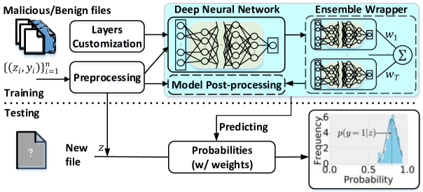
Figure 1. Our methodology for calibrating deep malware detectors to answer the aforementioned RQ1-RQ4, where dashed boxes indicate that the modules may not be necessary for some calibration methods. In the training phase, we learn the calibrated malware detectors. In the test phase, predicted probabilities (with weights if applicable) are obtained.

The preprocessing module transforms program files into the data formats that can be processed by deep learning models, including feature extraction and low-level feature representation. The layers customization module modifies the layers of standard deep learning models to incorporate appropriate calibration methods, such as placing a dropout layer before the input of the fully connected layer, the convolutional layer, or the LSTM layer; sampling parameters from learnable distributions. The deep neural network module constructs the deep learning models with the customized layers mentioned above to process the preprocessed data for training or testing purposes. The ensemble wrapper module uses an ensemble of deep learning models in the training and testing phases according to the incorporated calibration method. In this module, we load basic block models sequentially in the training and test phases for relieving the memory complexity. The model post-processing module copes with the requirements of post-hoc calibration methods. The input to this module is the detector’s output (i.e., predicted probability that a file belongs to which class) and a validation dataset (which is a fraction of data sampled from the same distribution as the training set). This means that this module does not affect the parameters $\theta$ of neural networks.

3.4. Selecting Metrics

In order to quantify the predictive uncertainty of a calibrated detector, we need to use a test dataset, denoted by $D_{test}$, and some metrics. In order to make the methodology widely applicable, we consider two scenarios: the ground-truth labels of testing dataset are available vs. are not available. It is important to make this distinction is important because ground-truth labels, when available, can be used to validate the trustworthiness of detectors’ predictive uncertainties. However, ground-truth labels are often costly to obtain, which motivates us to accommodate this more realistic scenario. This is relevant because even if the detector trainer may have access to ground-truth labels when learning detectors, these ground-truth labels may not be available to those that aim to quantify the detectors’ uncertainties in making predictions.

3.4.1. Selecting Metrics When Ground-Truth Labels Are Given

There are standard metrics that can be applied for this purpose. However, these metrics treat each example as equally important and are insensitive to data imbalance, which is often encountered in malware detection. This prompts us to propose variants of standard metrics to deal with the issue of data imbalance. Specifically, we use the following three predictive uncertainty metrics, which are applicable when ground-truth labels are known.

The first standard metric is known as Negative Log-Likelihood (NLL), which are commonly used as a loss function for training a model and intuitively measure the goodness of a model fitting the dataset (Candela et al., 2005). A smaller NLL value means a better calibration. Formally, this metric is defined as:

$$\mathbb{E}_{(z,y)\in D_{test}}-\left(y\log p(y=1|z,\theta)+(1-y)\log(1-p(y=1|z,\theta))\right).$$

In order to deal with imbalanced data, we propose using the following variant, dubbed Balanced NLL (bNLL), which is formally defined as: $\frac{1}{|\mathcal{Y}|}\sum_{i=0}^{|\mathcal{Y}|}\operatorname{NLL}(D_{test}^{i})$, where $\operatorname{NLL}(D_{test}^{i})$ is the expectation of negative log-likelihood on the test set $D_{test}^{i}$ of class $i$, $i\in\{0,1\}$. bNLL treats each class equally important, while NLL treats each sample equally.

The second standard metric is known as Brier Score Error (BSE), which measures the accuracy of probabilistic predictions (Brier, 1950; Snoek et al., 2019). A smaller BSE value means a better calibration. This metric is formally defined as: $\mathbb{E}_{(z,y)\in D_{test}}(y-p(y=1|z,\theta))^{2}$. In order to deal with imbalanced data, we propose using the following variant, dubbed balanced BSE (bBSE), which is formally defined as: $\frac{1}{|\mathcal{Y}|}\sum_{i=0}^{|\mathcal{Y}|}\operatorname{Brier}(D_{test}^{i})$, where $\operatorname{Brier}(D_{test}^{i})$ is the expectation of BSE on the test set $D_{test}^{i}$ of class $i$, $i\in\{0,1\}$.

The third standard metric is known as Expected Calibration Error (ECE), which also measures accuracy of predicted probabilities yet in a fine-grained manner (Naeini et al., 2015). A smaller ECE value means a better calibration. Formally, this metric is defined as follows. Given $S$ buckets corresponding to quantiles of the probabilities $\{\rho_{i}\}_{i=1}^{S}$, the ECE is defined as

(6) $$\text{ECE}=\sum_{s=1}^{S}\frac{B_{s}}{N}|\Pr(y=1|B_{s})-\text{conf}(B_{s})|,$$

where with a little abuse of notation, $B_{s}=\{(z,y)\in D_{test}:p(y=1|z,\theta)\in(\rho_{s},\rho_{s+1}]\}$ is the number of examples in bucket $s$, $\Pr(y=1|B_{s})=|B_{s}|^{-1}\sum_{(z,y)\in B_{s}}[y=1]$ is the fraction of malicious examples, $\text{conf}(B_{s})=|B_{s}|^{-1}\sum_{(z,y)\in B_{s}}{p(y=1|z,\theta)}$, and $N=|D_{test}|$. The ECE metric suffers from imbalanced data because the majority class dominates some bins owing to the weights $B_{s}/N$. In order to deal with imbalanced data, we propose using the following variant, dubbed Unweighted ECE (uECE), which is formally defined as follows.

$$\text{uECE}=\sum_{s=1}^{S}\frac{1}{S}|\Pr(y=1|B_{s})-\text{conf}(B_{s})|.$$

3.4.2. Selecting Metrics When Ground-Truth Labels Are Not Given

There are three metrics (Kendall and Gal, 2017; Pearce et al., 2020; Lakshminarayanan et al., 2017) that can be applied to quantify predictive uncertainty in the absence of ground-truth labels. These metrics are applied to a point (i.e., expectation is not considered), which indicates these metrics do not suffer from the imbalanced dataset.

The first metric is known as Entropy, which intuitively measure a state of disorder in a physical system (Kendall and Gal, 2017). A larger entropy value means a higher uncertainty; Formally, this metric is defined as:

(7) $$-(p(y|z,\theta)\log p(y|z,\theta)+(1-p(y|z,\theta))\log(1-p(y|z,\theta))),$$

where $p(y|z,\theta)$ denotes the model output $p(y=1|z,\theta)$ or Eq.(3).

The second metric is known as Standard Deviation (SD), which intuitively measures the inconsistency between the base classifiers and the ensemble one (Pearce et al., 2020). A larger SD value means a higher uncertainty. Formally, this metric is defined as:

$$\sqrt{\frac{T}{T-1}\sum_{i=1}^{T}w_{i}\left(p(y|z,\theta^{i})-p(y|z,\theta)\right)^{2}},$$

where $\theta^{i}$ denotes the $i$-th DNN model, which has a weight $w_{i}$ (ref. Eq.(5)) or $w_{i}=1/T$.

The third metric is known as the KL divergence, which is an alternative to SD (Lakshminarayanan et al., 2017). A larger KL value means a higher uncertainty. Formally, this metric is defined as:

$$\sum_{i=1}^{T}w_{i}(\operatorname{KL}(p(y|z,\theta^{i})||p(y|z,\theta))),$$

where $\operatorname{KL}$ denotes the Kullback-Leibler divergence.

3.5. Answering RQs

At this point, one can apply the calibrated detectors to quantify their predictive uncertainties. It should be clear that this methodology can be adopted or adapted by other researchers to conduct empirical studies with more kinds of detectors and more metrics.

4. Experimental Results and Analysis

4.1. Experimental setup

We implement the framework using TensorFlow (Abadi et al., 2016) and TensorFlow Probability libraries (Abadi et al., 2015) and run experiments on a CUDA-enabled GTX 2080 Ti GPU. We below detail datasets and hyperparameters.

4.1.1. Datasets

We use 3 widely-used Android datasets: Drebin (Arp et al., 2014), VirusShare (Corvus, 2020), and Androzoo (Allix et al., 2016).

Drebin: The Drebin dataset is built before the year of 2013 and is prepossessed by a recent study (Li and Li, 2020), which relabels the APKs using the VirusTotal service (Sistemas, 2020) that contains more than 70 antivirus scanners. An APK is treated as malicious if four or more scanners say it is malicious, and benign if no scanners say it is malicious; theoretical justification of such heuristic but widely-used practice has yet to be made (Du et al., 2018). The resultant Drebin dataset contains 5,560 malicious APKs and 42,333 benign APKs.

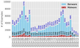
Figure 2. The Androzoo examples of APKs with time (Pendlebury et al., 2019).

VirusShare: VirusShare is a repository of potential malware. We chose the APKs collected in 2013 and treat this dataset as out-of-source in regards to the Drebin dataset. These APKs are labeled using the same fashion as the Drebin dataset, producing 12,383 malicious APKs and 340 benign APKs, while throwing away the 469 APKs in the grey area (i.e., at least one, but at most three, scanners say they are malicious).

Table 1. Detection estimation and uncertainty evaluation of calibrated malware detectors in the absence of dataset shift.

Malware detector	Calibration method	Detection estimation (%)					Uncertainty evaluation
		FNR	FPR	Acc	bAcc	F1	NLL	bNLL	BSE	bBSE	ECE	uECE
DeepDrebin	Vanilla	3.90	0.31	99.28	97.90	96.84	0.100	0.329	0.007	0.020	0.006	0.104
	Temp scaling	3.90	0.31	99.28	97.90	96.84	0.052	0.109	0.006	0.018	0.007	0.062
	MC Dropout	3.45	0.32	99.32	98.12	97.04	0.033	0.094	0.006	0.015	0.002	0.056
	VBI	3.36	0.83	98.88	97.91	95.22	0.054	0.094	0.009	0.016	0.012	0.102
	Ensemble	3.99	0.19	99.37	97.91	97.24	0.063	0.211	0.005	0.018	0.005	0.160
	wEnsemble	3.99	0.20	99.36	97.90	97.20	0.058	0.190	0.005	0.018	0.004	0.095
MultimodalNN	Vanilla	2.16	0.63	99.20	98.61	96.58	0.087	0.207	0.007	0.013	0.007	0.162
	Temp scaling	2.16	0.63	99.20	98.61	96.58	0.053	0.086	0.007	0.012	0.010	0.182
	MC Dropout	2.97	0.39	99.31	98.32	97.03	0.077	0.225	0.005	0.014	0.003	0.072
	VBI	8.45	0.33	98.73	95.61	94.35	0.073	0.253	0.010	0.036	0.004	0.078
	Ensemble	2.52	0.39	99.36	98.55	97.26	0.063	0.188	0.005	0.012	0.004	0.144
	wEnsemble	2.88	0.26	99.44	98.43	97.56	0.046	0.153	0.005	0.013	0.002	0.045
DeepDroid	Vanilla	8.53	0.69	98.41	95.39	92.99	0.097	0.311	0.013	0.039	0.009	0.059
	Temp scaling	8.53	0.69	98.41	95.39	92.99	0.076	0.220	0.013	0.038	0.002	0.023
	MC Dropout	7.62	0.66	98.54	95.86	93.57	0.078	0.239	0.012	0.035	0.004	0.055
	VBI	12.7	0.35	98.22	93.47	91.88	0.084	0.305	0.014	0.052	0.010	0.092
	Ensemble	7.44	0.11	99.05	96.23	95.73	0.049	0.171	0.008	0.029	0.006	0.162
	wEnsemble	4.99	0.27	99.18	97.37	96.41	0.050	0.131	0.007	0.022	0.008	0.066
Droidetec	Vanilla	4.14	1.53	98.17	97.17	92.30	0.119	0.208	0.016	0.026	0.014	0.205
	Temp scaling	4.14	1.53	98.17	97.17	92.30	0.101	0.167	0.016	0.026	0.015	0.180
	MC Dropout	3.03	1.40	98.41	97.78	93.32	0.088	0.142	0.014	0.020	0.013	0.207
	VBI	3.22	1.67	98.15	97.55	92.29	0.118	0.202	0.015	0.022	0.015	0.262
	Ensemble	3.13	0.75	98.98	98.06	95.60	0.055	0.107	0.009	0.016	0.010	0.143
	wEnsemble	3.49	0.59	99.07	97.96	95.98	0.046	0.101	0.007	0.016	0.008	0.116

Androzoo: Androzoo is an APK repository, including over 10 million examples, along with their VirusTotal reports. These APKs were crawled from the known markets (e.g., Google Play, AppChina). Following a previous study (Pendlebury et al., 2019), we use a subset of these APKs spanning from January 2014 to December 2016, which includes 12,735 malicious examples and 116,993 benign examples. Figure 2 plots the monthly distribution of these examples with time (Pendlebury et al., 2019).

4.1.2. Hyper-parameters

We present the hyper-parameters for malware detectors and then for calibration methods.

DeepDrebin (Grosse et al., 2017) is an MLP, consisting of two fully-connected hidden layers, each with 200 neurons.

MultimodalNN (Kim et al., 2019) has five headers and an integrated part, where each header consists of two fully-connected layers of 500 neurons. The integrated part consists of two fully-connected layers of 200 neurons.

DeepDroid (McLaughlin et al., 2017) has an embedding layer, followed by a convolutional layer and two fully-connected layers. The vocabulary of the embedding layer has 256 words, which correspond to 256 Dalvik opcodes; the embedding dimension is 8; the convolutional layer has the kernels of size 8$\times$8 with 64 kernels; the fully-connected layer has 200 neurons. Limited by the GPU memory, DeepDroid can only deal with a maximum sequence of length 700,000, meaning that APKs with longer opcode sequences are truncated and APKs with shorter opcode sequences are padded with 0’s (which correspond to nop).

Droidetec (Ma et al., 2020) has an embedding layer with vocabulary size 100,000 and embedding dimension 8, the bi-directional LSTM layer with 64 units, and a fully-connected hidden layer with 200 neurons. Droidetec allows the maximum length of API sequence 100,000. We further clip the gradient values into the range of [-100, 100] for Droidetec in case of gradient explosion.

All models mentioned above use the ReLU activation function. We also place a dropout layer with a dropout rate 0.4 before the last fully-connected layer (i.e., the output layer). We implement the four malware detectors by ourselves. The hyperparameters of calibration methods are detailed below.

Vanilla and Temp scaling: We have the same settings as the malware detectors mentioned above.

MC dropout: We use a dropout layer with a dropout rate 0.4. We add the dropout layer into the fully-connected layer, convolutional layer, and the LSTM layer, respectively. Following a recent study (Snoek et al., 2019), we neglect the $\ell_{2}$ regularization that could decline the detection accuracy. In the test phase, we sample 10 predictions for each example.

VBI: We sample the parameters of the fully-connected layer or the convolutional layer (i.e., weights and bias) from Gaussian distributions. A Gaussian distribution has the variables (mean and standard deviation), which are learned via back propagation using the reparameterization technique (Blundell et al., 2015). We do not implement VBI for Bi-LSTM, due to the effectiveness issue (Snoek et al., 2019; Wang et al., 2021). This means only the last layer of Droidetec is calibrated by VBI. In the test phase, we sample 10 predictions for each example.

Ensemble and wEnsemble: We learn 10 base instances for each ensemble-based method.

We learn these models using the Adam optimizer with 30 epochs, batch size 16, and learning rate 0.001. A model is selected for evaluation when it achieves the highest accuracy on the validation set in the training phase. In addition, we calculate the validation accuracy at the end of each epoch.

4.2. Answering RQ1

In order to quantify the predictive uncertainty of malware detectors in the absence of dataset shift, we learn the aforementioned 24 malware detectors on the Drebin dataset, by splitting it into three disjoint sets of 60% for training, 20% for validation, and 20% for testing.

Table 1 summarizes the results, including detection estimation using the metrics False Negative Rate (FNR), False Positive Rate (FPR), Accuracy (Acc) or percentage of detecting benign and malicious samples correctly, balanced Accuracy (bAcc) (Brodersen et al., 2010) and F1 score (Pendleton et al., 2016), and uncertainty evaluation using the metrics NLL, bNLL, BSE, bBSE, ECE, and uECE. We make four observations. First, Temp scaling achieves the same detection accuracy as its vanilla model because it is a post-processing method without changing the learned parameters. On the other hand, MC dropout, Ensemble and wEnsemble improve detection accuracy but VBI degrades detection accuracy somewhat when compared with the vanilla model. In terms of balanced accuracy, the calibration methods do not always improve detection accuracy because the vanilla MultimodalNN actually achieves the highest balanced accuracy 98.61% among all those detectors. The reason may be that MultimodalNN itself is an ensemble model (e.g., 5 headers are equipped).

Second, ensemble methods (i.e., Ensemble and wEnsemble) reduce the calibration error when compared with the respective vanilla models. Moreover, the two ensemble methods exceed the other calibration methods in terms of the NLL, BSE and bBSE metrics, except for DeepDrebin (suggesting MC Dropout is best for calibration). Third, the measurements of the balanced metrics are notably larger than their imbalanced counterparts (e.g., bNLL vs. NLL), because benign examples dominate the test set and malware detectors predict benign examples more accurately than predicting malicious ones.

Fourth, uECE shows inconsistent results in terms of bNLL and bBSE. In order to understand the reasons, we plot the reliability diagram (Niculescu-Mizil and Caruana, 2005), which demonstrates the difference between the fraction of malicious examples in each bin, namely the difference between the $\Pr(y=1|B_{s})$ in Eq.(6) and the mean of the predicted confidence $conf(B_{s})$. Figure 3 plots the results of the vanilla malware detectors, along with the number of examples in the bins. Figure 3a shows that most examples belong to bins $B_{1}$ and $B_{5}$. Figure 3b says DeepDroid achieves the lowest error (because it is closest to the diagonal than others), and shall be best calibrated, which contracts the ECE values in Table 1 (demonstrating that MultimodalNN is best instead). This is because as shown in Figure 3a, most benign examples belong to bin $B_{1}$ and most malicious examples belong to bin $B_{5}$. As a comparison, uECE does not suffer from this issue.

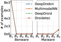
(a) # of examples per bin.

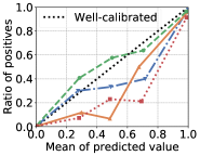
(b) Reliability diagram

Figure 3. Reliability diagram of vanilla malware detectors. There are 5 bins $B_{1},\ldots,B_{5}$ and “Benware” denotes the benign software.

Insight 1.

Calibration methods reduce malware detection uncertainty; variational Bayesian inference degrades detection accuracy and F1 score in the absence of dataset shift; balanced metrics (i.e., bNLL, bBSE and uECE) are more sensitive than their imbalanced counterparts (i.e., NLL, BSE and ECE) when data imbalance is present.

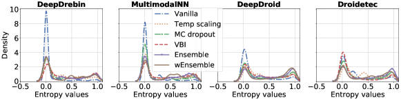
(a)

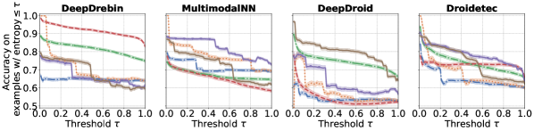
(b)

Figure 4. Predictive entropy (see Eq.(7)) of malware detectors trained on the Drebin dataset and tested on the VirusShare: (a) histogram of predictive entropy; (b) accuracy on the dataset after excluding the examples for which the detector has high uncertainties (i.e., the examples for which the predictive entropy is above a pre-determined threshold $\tau$), which corresponds to the real-world use of the quantified predictive uncertainty.

Table 2. Predictive uncertainty of malware detectors that are learned on the Drebin dataset and tested on the VirusShare.

	Calibration method	Detection(%)		Uncertainty evaluation
		Acc	bAcc	NLL	bNLL	BSE	bBSE	ECE	uECE
DeepDrebin	Vanilla	63.96	77.59	5.52	3.58	0.35	0.21	0.359	0.483
	Temp scaling	63.96	77.59	1.65	1.39	0.31	0.19	0.363	0.468
	MC Dropout	74.39	83.53	1.48	0.95	0.20	0.13	0.274	0.463
	VBI	82.69	87.07	0.64	0.52	0.13	0.10	0.210	0.434
	Ensemble	61.76	78.04	3.43	2.15	0.32	0.19	0.394	0.466
	wEnsemble	59.49	76.59	3.08	1.79	0.32	0.19	0.397	0.469
MultimodalNN	Vanilla	69.02	80.48	4.05	2.59	0.29	0.18	0.306	0.463
	Temp scaling	69.02	80.48	1.45	1.13	0.25	0.17	0.303	0.464
	MC Dropout	64.38	78.38	4.61	2.58	0.32	0.18	0.361	0.473
	VBI	58.17	77.21	2.32	1.25	0.33	0.18	0.414	0.478
	Ensemble	72.66	82.20	2.24	1.34	0.21	0.14	0.279	0.450
	wEnsemble	61.73	77.74	2.21	1.26	0.30	0.17	0.379	0.471
DeepDroid	Vanilla	52.85	70.02	3.44	2.11	0.42	0.27	0.463	0.481
	Temp scaling	52.85	70.02	2.09	1.31	0.39	0.25	0.460	0.477
	MC Dropout	65.50	74.22	1.54	1.10	0.26	0.20	0.338	0.465
	VBI	56.57	72.65	2.44	1.46	0.40	0.25	0.476	0.475
	Ensemble	56.57	72.65	1.78	1.12	0.33	0.20	0.435	0.475
	wEnsemble	64.11	74.22	1.22	1.00	0.24	0.19	0.350	0.461
Droidetec	Vanilla	59.98	70.04	2.22	1.59	0.34	0.253	0.389	0.476
	Temp scaling	59.98	70.04	1.66	1.20	0.32	0.235	0.390	0.476
	MC Dropout	64.99	72.61	1.57	1.33	0.27	0.222	0.344	0.472
	VBI	65.30	74.21	2.14	1.85	0.27	0.210	0.315	0.473
	Ensemble	63.83	72.45	1.33	0.94	0.24	0.185	0.343	0.470
	wEnsemble	62.26	71.64	1.50	1.23	0.28	0.219	0.375	0.465

4.3. Answering RQ2

In order to quantify the predictive uncertainty of malware detectors with respect to out-of-source examples, we apply the Drebin malware detectors to the VirusShare dataset. We assess predictive distribution and report the accuracy of malware detectors on the datasets obtained after removing the examples for which the detectors are uncertain (i.e., with an entropy value above a threshold $\tau$); this corresponds to the real-world usefulness of quantifying predictive uncertainty (i.e., discarding prediction results for which detector is uncertain).

Table 2 summarizes the uncertainty evaluation and the corresponding detection accuracy. We make three observations. (i) Malware detectors achieve low accuracy with out-of-source test examples. Nevertheless, DeepDrebin incorporating VBI obtain an accuracy of 82.69%, which notably outperforms other detectors. It is reminding that VBI hinders the detection accuracy in the absence of dataset shift. (ii) Calibration methods (e.g., VBI or Ensemble) reduce the uncertainty in terms of bNLL and bBSE when compared with the vanilla models, except for the MultimodalNN model incorporating MC dropout. (iii) DeepDrebin incorporating VBI also achieves the best calibration results, suggesting that VBI benefits from both regularization and calibration. On the other hand, DeepDroid and Droidetec suffer from the setting of out of source. Both models handle the very long sequential data that would be truncated due to the limited GPU memory, leading to the inferior results.

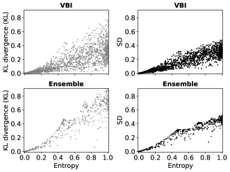
Figure 5. Scatter points of the randomly selected 2,000 test examples from the VirusShare dataset with paired values (Entropy, KL) and (Entropy, SD) that are obtained by applying DeepDrebin incorporating VBI or Ensemble.

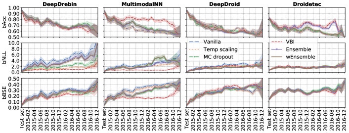
Figure 6. Illustration of balanced accuracy (bAcc), balanced NLL (bNLL), balanced BSE (bBSE) under temporal covariate shift.

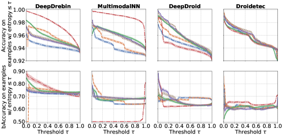
(a)

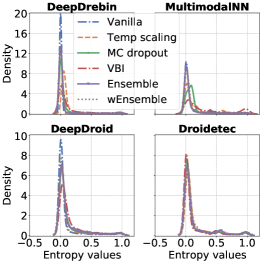
(b)

Figure 7. Predictive entropy (see Eq.(7)) of malware detectors on Androzoo dataset: (a) accuracy (upper row) and bAccuracy (bottom row) on the Androzoo test set after excluding the examples for which the detectors have high uncertainties (i.e., the examples for which the predictive entropy is above a pre-determined threshold $\tau$); (b) test sample density of predictive entropy.

Figure 4 illustrates the density of predictive entropy. Figure 4b further shows the accuracy on the examples after removing the ones for which the detectors are uncertain about their predictions. We make the following observations. (i) The vanilla models return zero entropy value for many examples, but calibration methods relieve this situation notably. Considering that the higher entropy delivers more uncertainty, vanilla model is poorly calibrated regarding the out-of-source examples. This is further confirmed that vanilla models exhibit a limited change along with increasing thresholds in Figure 4b. (ii) Ensemble and wEnsemble increase the robustness of deep learning models in detecting out-of-source examples. For example, the MultimodalNN, DeepDroid, and Droidetec models can be enhanced by Ensemble and wEnsemble to some extent, especially when applied to predicting the examples with entropy values below 0.3 (i.e., the detectors are relatively certain about their predictions). (iii) DeepDrebin incorporating either VBI or MC dropout make a significant achievement by comparing with ensemble-based calibrations. Because VBI requires suitable prior distributions, it is challenging to generalize this calibration to all models effectively (Blundell et al., 2015). (iv) Temp scaling demonstrates an un-intuitive phenomenon that it achieves almost 100% accuracy at the start of the curves when applied to DeepDrebin, MultimodalNN and Droidetec, but degrades the accuracy of DeepDroid. The is because Temp scaling tends to over-approximate the predicted probabilities, resulting in high confidence score for examples, some of which are mis-classified, however. In addition, the balanced accuracy demonstrates the similar experimental results (cf. the appendix materials for details).

Figure 5 plots the relationship between the entropy and the KL divergence (KL), and the relationship between the entropy and the Standard Deviation (SD). A scatter point represents a test example based on the paired value. We observe that these three measurements are closely related, which explains why we use the entropy to characterize the predictive uncertainty solely. We only report the results for the calibrated DeepDrebin with VBI and Ensemble, because similar phenomena are observed for the other models. Note that Vanilla and Temp scaling do not apply to KL divergence and standard deviation.

Insight 2.

Deep ensemble benefits calibration of malware detectors against out-of-source test examples, but a carefully tuned VBI model could achieve a higher quality of uncertainty than ensemble-based methods; Measurements of entropy, KL divergence and standard deviation are closely related.

Table 3. Effectiveness of calibrated malware detectors under adversarial evasion attacks.

Malware detector	Calibration method	No attack				“Max” PGDs+GDKDE attack				Mimicry attack
		Acc (%)	NLL	BSE	ECE	Acc (%)	NLL	BSE	ECE	Acc (%)	NLL	BSE	ECE
DeepDrebin	Vanilla	96.09	0.629	0.037	0.039	0.00	33.22	1.000	1.000	66.09	4.778	0.317	0.334
	Temp scaling	96.09	0.184	0.033	0.042	0.00	7.015	0.985	0.992	66.09	1.427	0.266	0.332
	MC Dropout	96.55	0.186	0.029	0.040	0.00	33.22	1.000	1.000	69.18	1.639	0.245	0.317
	VBI	96.27	0.142	0.025	0.051	0.00	33.22	1.000	1.000	69.91	1.034	0.211	0.320
	Ensemble	96.00	0.403	0.034	0.042	0.00	33.22	1.000	1.000	64.82	3.296	0.295	0.363
	wEnsemble	96.00	0.362	0.034	0.042	0.00	33.22	1.000	1.000	64.64	2.944	0.296	0.362
Multimo -dalNN	Vanilla	97.82	0.368	0.020	0.023	0.00	33.22	1.000	1.000	87.64	1.530	0.107	0.119
	Temp scaling	97.82	0.129	0.019	0.025	0.00	8.871	0.996	0.998	87.64	0.562	0.094	0.122
	MC Dropout	97.18	0.399	0.024	0.030	0.00	33.22	1.000	1.000	85.64	1.822	0.121	0.152
	VBI	96.82	0.166	0.026	0.042	0.00	33.22	1.000	1.000	89.64	0.506	0.080	0.119
	Ensemble	97.45	0.355	0.021	0.026	0.00	33.22	1.000	1.000	88.09	1.148	0.091	0.129
	wEnsemble	97.09	0.295	0.025	0.035	0.00	33.22	1.000	1.000	84.27	1.124	0.123	0.187
DeepDroid	Vanilla	91.55	0.587	0.073	0.095	85.45	0.773	0.116	0.148	86.09	0.786	0.110	0.142
	Temp scaling	91.55	0.404	0.069	0.113	85.45	0.536	0.105	0.165	86.09	0.538	0.101	0.158
	MC Dropout	92.55	0.451	0.066	0.097	93.55	0.273	0.048	0.074	90.18	0.529	0.083	0.126
	VBI	87.27	0.592	0.102	0.151	84.00	0.592	0.117	0.180	82.00	0.705	0.136	0.200
	Ensemble	92.55	0.329	0.058	0.099	90.64	0.366	0.068	0.129	89.55	0.433	0.079	0.142
	wEnsemble	95.00	0.237	0.040	0.069	93.00	0.309	0.057	0.111	92.82	0.348	0.061	0.111
Droidetec	Vanilla	98.08	0.123	0.016	0.028	66.03	2.331	0.298	0.341	88.80	0.656	0.099	0.126
	Temp scaling	98.08	0.113	0.017	0.039	66.03	1.717	0.285	0.345	88.80	0.514	0.095	0.138
	MC Dropout	98.81	0.063	0.009	0.018	67.30	2.066	0.272	0.330	93.17	0.268	0.052	0.090
	VBI	98.54	0.095	0.012	0.016	71.31	1.996	0.250	0.292	93.08	0.396	0.060	0.078
	Ensemble	99.18	0.060	0.008	0.014	80.87	0.657	0.138	0.215	96.17	0.175	0.030	0.068
	wEnsemble	99.00	0.048	0.008	0.015	80.05	0.776	0.151	0.232	95.90	0.156	0.029	0.066

4.4. Answering RQ3

In order to quantify the predictive uncertainty of malware detectors under temporal covariate shift, we use Androzoo dataset. Specifically, we train malware detectors upon the APKs collected in the year of 2014, and test these malware detectors upon APKs collected in the year of 2015 and 2016 at the month granularity. We also split the APKs in the year of 2014 into three disjoint datasets, 83.4% for training, 8.33% for validation (8.33% is the average percentage of APKs emerging in each month of 2014), and 8.33% for testing.

Figure 6 plots the balanced accuracy (bAccuracy), balanced NLL (bNLL) and balanced BSE (bBSE) under temporal covariate shift (more results are presented in the appendix materials). We make the following observations. (i) Malware detectors encounter a significantly decreasing of accuracy and increasing of bNLL and bBSE with newer test data. This can be attributed to the natural software evolution that Google gradually updates Android APIs and practitioners upgrade their APKs to support new services. In particular, Droidetec suffer a lot from temporal covariate shift and exhibits a low detection accuracy. As mentioned earlier, this may be that Droidetec is permitted to learn from a limited number of APIs, which inhibits handling the APKs with a broad range of APIs. (ii) Temp scaling has the same effect as the vanilla model in terms of bAccuracy; Ensemble enhances the vanilla models (DeepDrebin, MultimodalNN, and DeepDroid) at the start of several months but then this enhancement diminishes; VBI makes MultimodalNN to achieve the highest robustness under data evolution (but only achieves $\sim$80% bAccuracy). (iii) Ensemble methods benefit calibration in terms of bNLL and bBSE when compared with the vanilla model; VBI incorporating DeepDrebin or MultimodalNN achieves an impressive result.

Figure 7a plots the accuracy (at the upper half) and the balanced accuracy (at the lower half) after excluding the examples for which the detectors have entropy values greater than a threshold $\tau$. Figure 7b plots the sample density of predictive entropy. We observe that (i) either accuracy or balanced accuracy decreases dramatically when the entropy increases, which is particularly true for DeepDroid and Droidetec. (ii) MultimodalNN incorporating VBI seems to work very well in terms of accuracy, but not necessary for balanced Accuracy. This is because the model classifies most benign samples correctly but not malicious ones until the threshold value is approach 0.9. Moreover, it is interesting to see that MultimodalNN incorporating VBI achieves the best bAccuracy without considering uncertainty (cf. Figure 6, which is in sharp contrast to Figure 7a). The reason behind this is that MultimodalNN incorporating VBI correctly classifies a portion of examples with high entropy value, as shown in Figure 7b. (iii) DeepDrebin incorporating VBI outperforms the other Drebin-based models, which resonates the results obtained in our second group of experiments (cf. Figure 4b in Section 4.3). (iv) Figure 7b says that for all of the malware detectors except MultimodalNN incorporating VBI and DeepDrebin incorporating VBI, most examples tend to have a small entropy. This suggests ineffective calibrations of malware detectors under temporal covariate shifts and a lack of good calibration method.

Insight 3.

Calibrated malware detectors cannot cope with temporal datashit shift effectively, but VBI is promising for calibration and generalization under temporal covariate shift.

4.5. Answering RQ4

In order to quantify the predictive uncertainty of malware detectors under adversarial evasion attacks, we wage transfer attacks and generate adversarial APKs via a surrogate DeepDrebin model. We do not include adversarial APKs with respect to MultimodalNN, DeepDroid, and Droidetec because we do not find effective solutions. The surrogate DeepDrebin model consists of two fully-connected layers of 160 neurons with the ReLU activation function. We learn the model using the Adam optimizer with learning rate 0.001, batch size 128, and 150 epochs. We then generate adversarial examples against the surrogate model to perturb the 1,112 malicious APKs in the test dataset. Specifically, by following a recent study (Li and Li, 2020), we first perturb the feature vectors of the APKs using the “max” PGDs+GDKDE attack and the Mimicry attack, and then obtain adversarial APKs by using obfuscation techniques. In total, we obtain 1100 perturbed APK files for both attacks, respectively.

Table 3 summarizes the results of the malware detectors under the “max” PGDs+GDKDE attack and the Mimicry attack. Because the test dataset contains malware samples solely, we consider the Accuracy, NLL, BSE and ECE rather than their balanced versions. We observe that (i) the “max” PGDs+GDKDE attack renders DeepDrebin and MultimodalNN models useless, regardless of the calibration methods. Nevertheless, DeepDroid is robust against this attack because opcode are not used by the DeepDrebin and thus is unfocused by the attacker. However, DeepDroid still suffers somewhat from this attack because of the opcode manipulations is leveraged for preserving the malicious functionality. (ii) Under the Mimicry attack, VBI makes DeepDrebin and MultimodalNN achieve the best accuracy and the lowest calibration error (in terms of NLL and BSE), while weighted Ensemble makes both obtain the worst results. However, this situation is changed in regards to DeepDroid and Droidetec. This might be that DeepDrebin and MultimodalNN are more sensitive to Mimicry attack than DeepDroid and Droidetec, leading to that an ensemble of vulnerable models decreases the robustness against the attack.

Insight 4.

Adversarial evasion attacks can render calibrated malware detectors, and therefore the quantified predictive uncertainty, useless, but heterogeneous feature extraction does improve the robustness of malware detectors against the transfer attacks.

5. Conclusion

We empirically quantified the predictive uncertainty of four deep malware detectors with six calibration strategies (i.e., 24 detectors in total). We found that the predictive uncertainty of calibrated malware detectors is useful except for adversarial examples. We hope this study will motivate and inspire more research in quantifying the uncertainty of malware detectors, which is of paramount importance in practice but it is currently little understood.

Appendix A Experimental Results on the VirusShare Dataset

Figure 8 plots the balanced accuracy on the VirusShare dataset with decision referral. We observe that Figure 8 exhibit the trends that are similar to what are exhibited by Figure 4b, except for Temp scaling on DeepDrebin and MultimodalNN. This is because the model predicts benign examples accurately, but do not predict malicious examples accurately.

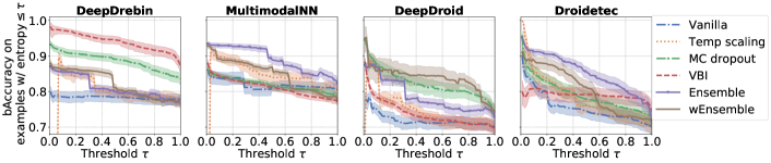
Figure 8. The balanced accuracy on the VirusShare dataset after excluding the examples for which the detector has high uncertainties (i.e., the examples for which the predictive entropy is above a pre-determined threshold $\tau$). For each curve, a shadow region is obtained from the 95% confidence interval using a bootstrapping with $10^{3}$ repetitions and sampling size being the number of examples in the VirusShare dataset.

Appendix B Experimental Results on the Androozoo Dataset

Figure 9 plots the Accuracy, NLL and BSE of malware detectors under temporal covariate shifts. We observe that the Accuracy, NLL, and BSE are smaller than their balanced counterparts plotted in Figure 6, owing to the data imbalance exhibited by the Androzoo dataset, despite that they all exhibit a similar trend.

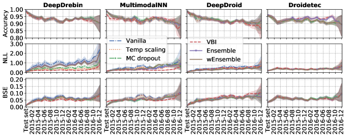
Figure 9. Illustration of accuracy, NLL, BSE under temporal covariate shift on the Androzoo dataset. A shadow region is obtained from the 95% confidence interval using a bootstrapping with $10^{3}$ repetitions and sampling size being the number of APKs in per month (cf. Figure 2).