Asymptotic Causal Inference

Abstract

We investigate causal inference in the asymptotic regime as the number of variables $n\rightarrow\infty$ using an information-theoretic framework. We define structural entropy of a causal model in terms of its description complexity measured by the logarithmic growth rate, measured in bits, of all directed acyclic graphs (DAGs) on $n$ variables, parameterized by the edge density $d$. Structural entropy yields non-intuitive predictions. If we randomly sample a DAG from the space of all models over $n$ variables, as $n\rightarrow\infty$, in the range $d\in(0,\frac{1}{8})$, almost surely ${\cal D}$ is a two-layer DAG! Semantic entropy quantifies the reduction in entropy where edges are removed by causal intervention. Semantic causal entropy is defined as the $\phi$-divergence $D_{\phi}(P\parallel P_{S})$ between the observational distribution $P$ and the interventional distribution $P_{S}$, where a subset $S$ of edges are intervened on to determine their causal influence. We compare the decomposability properties of semantic entropy for different choices of $\phi$, including $\phi(t)=t\log t$ (KL-divergence), $\phi=\frac{1}{2}(\sqrt{t}-1)^{2}$ (squared Hellinger distance), and $\phi=\frac{1}{2}|t-1|$ (total variation distance). We apply our framework to generalize a recently popular bipartite experimental design for studying causal inference on large datasets, where interventions are carried out on one set of variables (e.g., power plants, items in an online store), but outcomes are measured on a disjoint set of variables (residents near power plants, or shoppers). We generalize bipartite designs to $k$-partite designs, and describe an optimization framework for finding the optimal $k$-level DAG architecture for any value of $d\in(0,\frac{1}{2})$. As $d$ increases, a sequence of phase transitions occur over disjoint intervals of $d$, with deeper DAG architectures emerging as $d\rightarrow\frac{1}{2}$. We also give a quantitative bound on the number of samples needed to reliably test for average causal influence for a $k$-partite design.

1 Introduction

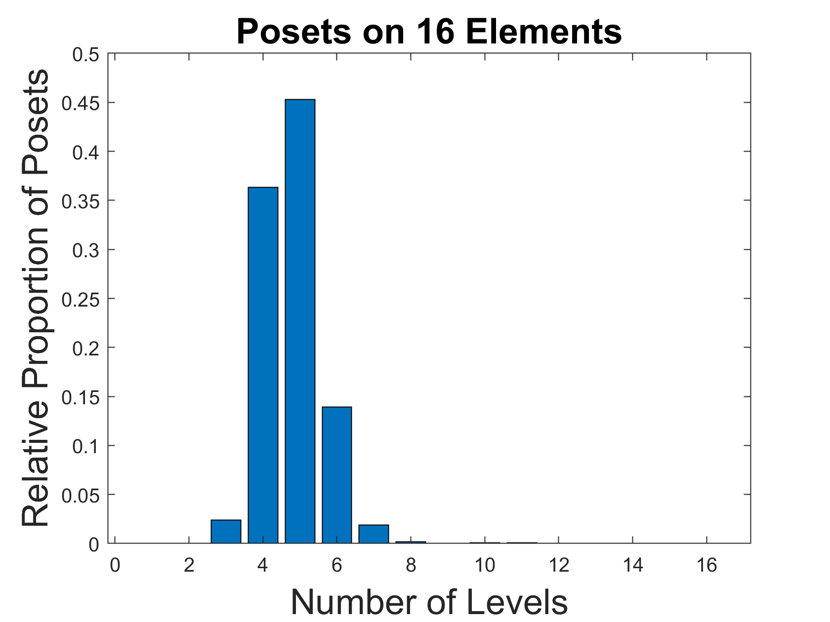
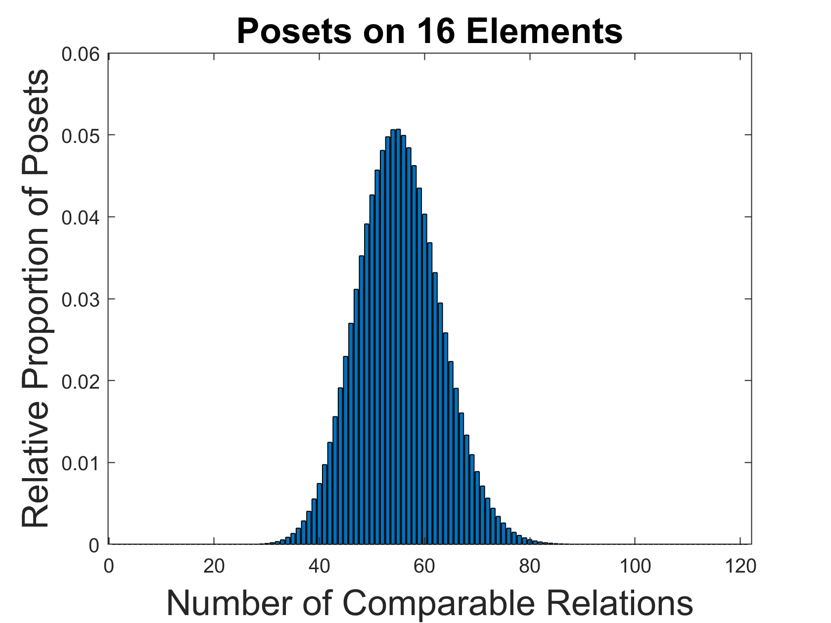
Figure 1: The relative proportion of non-isomorphic posets (or DAGs) on $16$ elements as a function of the number of levels (left) and the number of relations or edges (right). Note the highly peaked distribution: randomly sampling the space of $16$-variable models will with high probability generate a DAG of $4-6$ levels with $50-70$ comparable relations. Plots based on tables in (Brinkmann and McKay, 2002).

Inspired by a range of asymptotic studies, from neural tangent kernels (Jacot et al., 2018) to random graphs (Frieze and Tkocz, 2020) and phase transition effects in satisfiability problems (Bailey et al., 2007), we investigate causal inference in a novel regime as the number of variables $n\rightarrow\infty$. In contrast, most previous work that has investigated the non-asymptotic case (Pearl, 2009; Spirtes et al., 2000; Eberhardt, 2008; Hauser and Bühlmann, 2012; Kocaoglu et al., 2017; Mao-cheng, 1984; Tadepalli and Russell, 2021; Daskalakis and Pan, 2017). Our approach is motivated by the need to scale causal inference to real-world applications in diverse areas such as improving healthcare outcomes by reducing pollution, social network analysis, recommender systems, online ad placement, and two-sided platforms for dynamic pricing, which may involve building models over potentially millions of variables (Li et al., 2020; Pouget-Abadie et al., 2019; Schlosser and Boissier, 2018; Schlosser et al., 2018; Rödder et al., 2019; Charles et al., 2010; Zigler and Papadogeorgou, 2018). We define an information-theoretic framework based on an evolutionary process of growth and decay of the relative proportion $O(dn^{2})$ of edges (or relations) in the causal model. Structural causal entropy, or model description complexity, quantifies the evolutionary growth in the number of models, where we build on some classic results in extremal combinatorics of partially ordered sets (posets) (Dhar, 1978; Kleitman and Rothschild, 1979; Prömel et al., 2001b). Semantic entropy, in contrast, quantifies the reverse evolutionary process of the decay in the relative proportion of edges due to causal intervention. In particular, we build on the information-theoretic paradigm for quantifying causal influence (Massey and Massey, 2005; Wieczorek and Roth, 2019; Raginsky, 2011; Ay and Polani, 2008; Janzing et al., 2013). We use the edge-centric paradigm of causal intervention proposed in (Janzing et al., 2013), except we generalize their approach to using a general $\phi$-divergence.

If we imagine causal discovery as nature generating data from a randomly chosen causal model from the space of all possible causal DAG models on $n$ variables, as $n\rightarrow\infty$, surprisingly, almost surely the DAG has a very small number of levels (see Figure 1). (Kleitman and Rothschild, 2001) derived upper bounds on the logarithmic growth rate of DAGs and their associated posets ${\cal P}_{n}$, as $n\rightarrow\infty$. Their analysis showed that that the class of all $n$-layer DAG models ${\cal P}_{n}$ is dominated in the limit by a subclass of DAG models ${\cal Q}_{n}$ with just three layers, more precisely $|{\cal P}_{n}|\leq(1+\frac{1}{o(n)})|{\cal Q}_{n}|$. (Dhar, 1978) investigated posets parameterized by the number $d\in(0,1)$ comparable pairs, and showed that posets can model lattice gas with energy proportional to the number of comparable pairs in the poset. Remarkably, phase transition effects appear as $d$ is varied. If we design a causal study that generates data from a uniformly randomly sampled DAG ${\cal D}\sim P({\cal P}_{n})$ over the space of all DAG models, in the range $d\in(0,\frac{1}{8})$, as $n\rightarrow\infty$, Dhar’s results imply that almost surely ${\cal D}$ is a two-layer DAG.

Semantic causal entropy, in contrast, attempts to quantify the reverse evolutionary process of decay of the proportion of edges $dn^{2}$ due to causal interventions that eliminate edges. A variety of information-theoretic metrics have been proposed to quantify causal influence (Massey and Massey, 2005; Raginsky, 2011; Ay and Polani, 2008; Wieczorek and Roth, 2019). We generalize the edge-centric model proposed by (Janzing et al., 2013), and define causal influence of removing a set of edges $S$ as the $\phi$ divergence $D_{\phi}(P\parallel P_{S})$ between the distribution $P$ represented by the original DAG with $P_{S}$ denoting the distribution represented by the DAG with edges $S$ removed. If $\phi(t)=t\log t$, we recover the model proposed by (Janzing et al., 2013). For $t=2(1-\sqrt{t})$, we get the intervention model proposed by (Daskalakis and Pan, 2017), and for $t=\frac{1}{2}|t-1|$, we get the model proposed by (Acharya et al., 2018). These choices lead to different decomposability properties for quantifying causal influence. We generalize recent bipartite designs for studying causal inference on large datasets, where interventions are carried out on one set of variables (e.g., power plants, items in an online store), but outcomes are measured on a disjoint set of variables (residents near power plants, or shoppers) (Li et al., 2020; Pouget-Abadie et al., 2019; Schlosser and Boissier, 2018; Schlosser et al., 2018; Rödder et al., 2019; Charles et al., 2010; Zigler and Papadogeorgou, 2018). We propose a class of $k$-partite architectures, where the variables are partitioned into $[n]=X_{1}\sqcup\ldots X_{k}$ antichains, and describe an optimization framework for finding the $k$-level DAG architecture for any value of $d\in(0,\frac{1}{2})$ that maximizes causal entropy, which reveals a sequence of phase transitions occur for disjoint intervals of $d$, with deeper DAG architectures emerging as $d\rightarrow\frac{1}{2}$. We give a provably quantitative estimate of the number of samples needed to measure the average causal influence from a set of edges for $k$-partite designs.

2 Semantic Entropy using Average Causal Influence

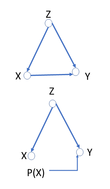
• Causal influence ${\cal C}^{\phi}_{S}=D_{\phi}(P\parallel P_{S})$, for some set of edges $S$, is defined as the $\phi$-divergence between the original pre-intervention distribution $P$ with the post-intervention distribution $P_{S}$.

• For the DAG on the left, the pre-intervention distribution $P(x,y,z)=P(z)P(x|z)P(y|x,z)$, and the post-intervention distribution $P_{X\rightarrow Y}(x,y,z)=P(z)P(x|z)\sum_{x^{\prime}}P(y|x^{\prime},z)P(x^{\prime})$.

• If $\phi(t)=t\log t$, then $C^{KL}_{X\rightarrow Y}=\sum_{x,y,z}P(x,y,z)\log\frac{P(y|x,z)}{\sum_{x^{\prime}}P(y|z,x^{\prime})P(x^{\prime})}$,

• If both edges were included in the intervention set $T=\{(Z,X),(Z,Y)\}$, then the post-intervention distribution is simply equal to $P_{T}(x,y,z)=P(x)P(y)P(z)$.

• If $X$ is simply a copy of $Z$, and $Y$ computes the XOR function of $X$ and $Z$, then if $P(Z=0)=a,P(Z=1)=1-a$, then then ${\cal C}^{KL}_{S}(P)=H(a)$, the entropy of $a$.

Figure 2: We define causal influence in terms of the $\phi$-divergence between the original distribution and the intervened distribution. We are particularly interested in choices of $\phi$, for which causal influences are decomposable. For $\phi=t\log t$, we obtain the $D_{KL}(P\parallel P_{S})$ causal influence model proposed by (Janzing et al., 2013). For $\phi(t)=\frac{1}{2}(\sqrt{t}-1)^{2}$, we get the squared Hellinger distance model $D_{H^{2}}(P\parallel P_{S})$ studied by (Daskalakis and Pan, 2017). Finally, for $\phi(t)=\frac{1}{2}|t-1|$, we get the total variation distance model $D_{TV}(P\parallel P_{S})$ studied by (Acharya et al., 2018). To get some intuition for the edge-centric causal influence model, in the above DAG, if $Z$ is age, $X$ is a covid vaccine, and $Y$ is getting infected, then the causal influence ${\cal C}_{X\rightarrow Y}$ associated with removing edge $X\rightarrow Y$ measures the difference between the infection rate where vaccination rates are allowed to depend on self-selection across age groups – for example, older people may choose to vaccinate more than younger people – versus the infection rate arising from a randomized vaccination strategy independent of age.

Generally, causal discovery (Pearl, 2009; Spirtes et al., 2000) is often modeled as inferring a DAG structure ${\cal G}_{n}=(V_{n},E_{n})$ (Pearl, 1989), where $V_{n}=[n]=\{1,\ldots,n\}$, based on observations and interventions. Variables will be denoted in upper case, e.g. $X_{i}$, whereas their values will be denoted in lower case, such as $x_{i}$. The edge set $E_{n}$ is a set $\{(x,y)\in V_{n}\times V_{n}\ |\ (x,y)\in E_{n}\}$, where $x,y\in[n]$, of comparable pairs. Our focus is understanding the asymptotic case where a DAG is randomly sampled from the space of all DAGs on $n$ variables, as $n\rightarrow\infty$. We use an edge-centric intervention model (see Figure 2) (Janzing et al., 2013), which differs from the more common node-centric models used in much previous work (Pearl, 2009; Eberhardt, 2008; Hauser and Bühlmann, 2012; Kocaoglu et al., 2017; Mao-cheng, 1984; Tadepalli and Russell, 2021; Daskalakis and Pan, 2017; Acharya et al., 2018).

Definition 1.

Let $\Phi^{*}$ be the set of all convex functions $\phi(t),t\geq 0$, such that at $t=1,\phi(1)=0$, and at $t=0,0\phi(\frac{0}{0})=0$. The $\phi$-divergence(CSISZÁR, 1967) $D_{\phi}(P\parallel Q)$ for two discrete distributions $P$ and $Q$ is

$$D_{\phi}(P\parallel Q)=\sum_{i}q_{i}\phi\left(\frac{p_{i}}{q_{i}}\right)$$ (1)

and for the continuous case (where the $\phi$-divergence is independent of the dominating measure $\mu$):

$$D_{\phi}(P\parallel Q)=\int_{q>0}\phi\left(\frac{p(x)}{q(x)}\right)\ q(x)\ d\mu(x)$$ (2)

Definition 2.

The causal influence ${\cal C}^{\phi}_{S}$ of a set of edges $S\subset E_{n}$ in a DAG $G_{n}=([n],E_{n})$ is defined as the $\phi$-divergence $D_{\phi}(P\parallel P_{S})$, for some convex function $\phi$, where $\phi(1)=0$, and where $P$ is the original pre-intervention distribution and $P_{S}$ is the post-intervention distribution, defined as follows:

$$P(x_{1},\ldots,x_{n})=\prod_{i=1}^{n}P(x_{i}|\mbox{pa}_{i})$$ (3)

where $\mbox{Pa}_{i}$ is the set of parent variables of $X_{i}$ (and $\mbox{pa}_{i}$ are their specific instantiations). Given a set of edges $S$ whose causal influence is to be quantified, the post intervention distribution $P_{S}$ is defined as:

$$P_{S}(x_{1},\ldots,x_{n})=\prod_{i=1}^{n}P_{S}(x_{i}|\mbox{pa}^{\bar{S}}_{i})=\prod_{i=1}^{n}\sum_{\mbox{pa}^{S}_{i}}P(x_{j}|\mbox{pa}^{\bar{S}},\mbox{pa}^{S}_{i})P_{\Pi}(\mbox{pa}^{S}_{j})$$ (4)

where $S=\{(i,j)\in E_{n}\}$ is the set of edges intervened on, $\bar{S}=\{(i,j)\notin S\}$ are the non-intervened edges, $\mbox{Pa}^{S}_{i}$ is the set of parents of variable $X_{i}$ whose edges are included in $S$, $\mbox{Pa}^{\bar{S}}_{i}$ are the parents of variable $X_{i}$ whose edges are not included in $S$, and $P_{\Pi}(\mbox{pa}^{S}_{i})$ is the product of marginal distributions of all variables in $\mbox{Pa}^{S}_{i}$.

Definition 3.

The causal influence $C_{X\rightarrow Y}(P)$ is localizable if the strength of $X\rightarrow Y$ only depends on knowing $P(Y|\mbox{PA}_{Y})$ and $P(\mbox{PA}_{Y})$.

Definition 4.

Given a set of edges $S$, $\mbox{trg}(S)=\{X_{i}|(X_{j},X_{i})\in S\}$ denotes the target nodes of the intervention.

(Janzing et al., 2013) defined causal influence and localizability specifically for $D_{KL}(P\parallel P_{S})$. Below we show that this notion can be significantly generalized to several other types of $\phi$ divergences, which lead to different decomposability properties, as summarized by the following result.

Theorem 1.

The causal influence ${\cal C}^{\phi}_{S}=D_{\phi}(P\parallel P_{S})$ of a set of edges $S\subset E_{n}$ in a DAG $G_{n}=([n],E_{n})$ has the following decomposability properties, depending on choice of $\phi$:

• $\phi=t\log t$: Using the chain rule for KL-divergences, it can be shown that $C^{KL}_{S}(P)=\sum_{i}D_{KL}(P\parallel P_{S_{i}})=\sum_{X_{i}\in\mbox{trg}(S)}D_{KL}(P(X_{i}|PA_{i})\parallel P_{S}(X_{i}\parallel\mbox{PA}_{i})$. This result was shown in (Janzing et al., 2013).

• $\phi=\frac{1}{2}(\sqrt{t}-1)^{2}$ or $t=\frac{1}{2}|t-1|$: In these cases, corresponding to squared Hellinger distance and total variation distance, the results of (Daskalakis and Pan, 2017) and (Acharya et al., 2018) imply that the resulting causal influences are subadditive

  $${\cal C}^{\phi}_{S}=D_{\phi}(P\parallel P_{S})\leq\sum_{X_{i}\in\mbox{trg}(S)}D_{\phi}(P_{X_{i}\cup\mbox{Pa}_{i}}\parallel P_{X_{i}\cup\mbox{Pa}^{\bar{S}}_{i}})$$ (5)

(Ding et al., 2021) give a detailed analysis of subadditivity properties of various other $\phi$-divergences, including $\chi^{2}$, Wasserstein distance, Jensen-Shannon divergences and several others. As we show later, a key strength of squared Hellinger distance and total variation distance over KL divergence is that the former metrics provide sample-efficient testing methods (Acharya et al., 2018; Daskalakis and Pan, 2017). A well-known result relates the above three $\phi$ divergences, showing they are closely related.

Lemma 1.

For any two distributions $P$ and $Q$, the following well-known inequalities hold (Sason and Verdú, 2015):

$$D_{TV}(P\parallel Q)\leq\sqrt{2}\ D_{H^{2}}(P\parallel Q)\leq\sqrt{D_{KL}(P\parallel Q)}$$ (6)

Similar to the standard notion of average treatment effect in the Neyman-Rubin potential outcomes framework (Imbens and Rubin, 2015), we can define the average causal influence of a set of edges $S$:

Definition 5.

Average causal influence $ACI^{\phi}(S)$ of a set of edges $S\subset E_{n}$ in a DAG $G_{n}=([n],E_{n})$ is defined as the average $\phi$-divergence $\frac{1}{|S|}D_{\phi}(P\parallel P_{S})$, where $P$ is the original pre-intervention distribution and $P_{S}$ is the post-intervention distribution.

3 Causal Structural Entropy and Phase Transitions

Causal edge interventions remove edges, and reduce the number of comparable relations. We now look at the growth of edges as the proportion of comparable relations $d$ increases from $0$ to $\frac{1}{2}$. Structural entropy of a causal model captures its description complexity, defined as $c(d)\equiv\lim_{n\rightarrow\infty}\frac{\log_{2}|{\cal P}^{d}_{n}|}{n^{2}}$, the limit of the logarithmic growth rate, measured in bits, of a directed acyclic graph (DAG) (or equivalently, the induced partially ordered set) on $n$ variables ${\cal P}^{d}_{n}$, parameterized by the relative proportion $d\in(0,1)$ of the total $dn^{2}$ edges in the DAG (or relations in the poset). It is well known that the set of possible DAG structures on $n$ variables grows superexponentially (Robinson, 1977). Surprisingly, it turns out that longstanding results in extremal combinatorics on the structure of partially ordered sets (Dhar, 1978, 1980; Kleitman and Rothschild, 2001; Prömel et al., 2001b) gives insights into the structure of DAG models in high-dimensional spaces.

Definition 6.

Let ${\cal P}_{n}$ denote the family of labeled posets on the point set $[n]$, where a particular poset $P\in{\cal P}_{n}$ is defined as a set of comparable pairs $(x,y)\in P$ iff $x\leq y$, and $x<y$ if $x\leq y$ and $x\neq y$. We say $x$ is covered by $y$ if $x<y$ and there is no other element $z$ such that $x<z$ and $z<y$. The cover graph associated with a poset $P$ is the directed graph $G_{P}=([n],E_{P})$ whose edges $E_{P}$ are defined by the cover relationship of the poset.

Definition 7.

The Hasse diagram ${\cal H}_{P}$ of a poset $P$ is a DAG with vertices $[n]$, and a single directed edge from $a\rightarrow b$ if and only if $a$ covers $b$. Distinct posets in ${\cal P}_{n}$ define distinct graphs. A Hasse diagram is in fact a DAG, as it cannot have any directed cycles, which would violate transitivity. In particular, Hasse diagrams are defined to contain no triangles either, that is $a\rightarrow b,b\rightarrow c,a\rightarrow c$. A node $a$ is adjacent to $b$ in a Hasse diagram if $a$ covers $b$ or $b$ covers $a$.

Definition 8.

The levels of a Hasse diagram ${\cal H}_{P}$ of a poset $P$ is defined as follows. Level 1 consists of all minimal vertices of ${\cal H}_{P}$, that is vertices that are not covering any other vertex. For each $j>1$, level $j$ is the set of minimal vertices obtained by deleting all vertices in levels $1,\ldots,j-1$. If $a$ is in level $i$, and $b$ is in level $j$, if $i<j$, then either $a<b$ or $a$ and $b$ are incomparable. Two vertices at the same level are necessarily incomparable, consequently vertices at a level form an antichain.

Definition 9.

Given a poset $P$ on $[n]$, a chain ${\cal C}\subset[n]$ is defined to be a totally ordered subset of $P$. The height of a poset is defined as the maximum cardinality of a chain. An antichain ${\cal A}\subset[n]$ of a poset $P$ is a subset of elements in which no pair of elements are ordered. The set of all elements $[n]$ can be partitioned into disjoint subsets of chains or antichains, whose sizes are related by Mirsky’s theorem (Mirsky, 1971), which simply states that the number of antichains is lower bounded by the number of chains, as no two elements of a chain can ever be in an antichain.

Theorem 2.

Mirsky’s theorem (Mirsky, 1971): The height of a partial ordering $P$ is defined to be the maximum cardinality of a chain, a totally ordered subset of the given partial order. For every partial ordering $P$, its height also equals the minimum number of antichains.

The challenge in combinatorial enumeration is obtaining good upper bounds on the size of ${\cal P}_{n}$, but lower bounds are of course much easier.

Theorem 3.

The number of posets ${\cal P}_{n}$ on a finite set $[n]$ is $|{\cal P}_{n}|\geq 2^{\frac{n^{2}}{4}}$.

Proof: Fix two antichains $X$ and $Y$, each on $\frac{n}{2}$ points, and for each of the $\frac{n^{2}}{4}$ comparable pairs $(x,y)\in X\times Y$, decide if $x\leq y$ or $y\leq x$. ∎

Upper bounding the number of posets ${\cal P}_{n}$ is much harder. To develop some intuition, let us consider a canonical representation of posets that will be used in the remainder of the paper.

Definition 10.

Define the class of $k$-partitioned models (DAGs or posets) as ${\cal Q}^{k}_{n}$ where the elements $[n]=V_{1}\sqcup V_{2}\ldots V_{k}$ form a disjoint class of $k$ partitions, satisfying the following conditions:

1. If $x\in V_{i}$ and $y\in V_{j}$, with $x<y$, then $i<j$.

2. If $x\in V_{i}$ and $y\in V_{j}$ and $i<j-1$, then $x<y$.

Condition 1 above ensures the antichain elements are not comparable. Condition 2 restricts the poset so that each element at level $L_{i}$ is comparable to every element at level $L_{i+2}$, where $1\leq i\leq k-2$. This second restriction is imposed to make the enumeration simpler, but as it will turn out, these restricted models in fact completely characterize the space of all posets on $n$ variables, as $n\rightarrow\infty$.

Theorem 4.

The number of $k$-partite causal models is $|{\cal Q}^{k}_{n}|\sim 2^{\sum_{i=1}^{k-1}|V_{i}||V_{i+1}|}$

Proof: Given the conditions imposed by Definition 10, the only freedom in generating a poset is choosing the relations between the elements in $V_{i}$ and $V_{i+1}$, for $1\leq i\leq k-1$. Note that we are ignoring the number of ways of distributing the elements in each antichain, as it only adds factors of size $o(n)$ to the exponent. ∎

A useful property that links combinatorics and entropy is given by the following lemma.

Lemma 2.

For any fixed $0<x<1,{n\choose nx}=2^{H(x)n+o(n)}$.

Theorem 5.

(Kleitman and Rothschild, 2001) proved the following classic upper bound:

$$\log_{2}|{\cal P}_{n}|=\frac{n^{2}}{4}+\frac{3n}{2}+\mathcal{O}(\log_{2}(n))$$ (7)

Sketch of Proof: (Kleitman and Rothschild, 2001) classified the set of all DAG models (Hasse diagrams of posets) in ${\cal P}_{n}$ into $15$ disjoint classes, and show that the class of all models, in the limit as $n\rightarrow\infty$, was dominated by one particular subclass of DAGs ${\cal Q}_{n}$ with exactly three levels defined below. ∎

Definition 11.

The class of three layer DAG models ${\cal Q}_{m+1}$ on $[m+1]$ elements is defined as follows.

1. The set of variables $V$ in ${\cal Q}_{m+1}$ is decomposed as $V=V_{1}\sqcup V_{2}\sqcup V_{3}$, where $V_{1}$, $V_{2}$, and $V_{3}$ are the three antichains of the poset.

2. For levels $i=1,3$, $\frac{m+1}{4}-\sqrt{m}\log m<|V_{i}|<\frac{m+1}{4}+\sqrt{m}\log m$

3. For level $2$, $\frac{m+1}{2}-\log m<|V_{2}|<\frac{m+1}{2}+\log m$

Theorem 6.

The set of all posets ${\cal P}_{n}$ is such that $|{\cal P}_{n}|=(1+\mathcal{O}(\frac{1}{n})|{\cal Q}_{n}|$. Informally, all causal models in the limit are essentially three layer DAGs!.

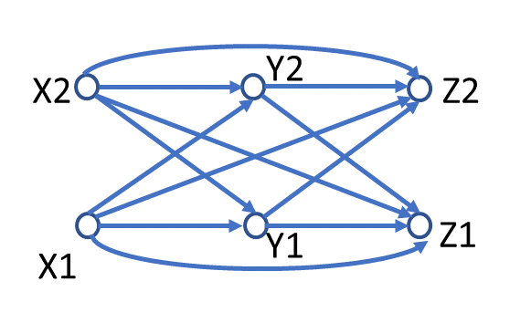
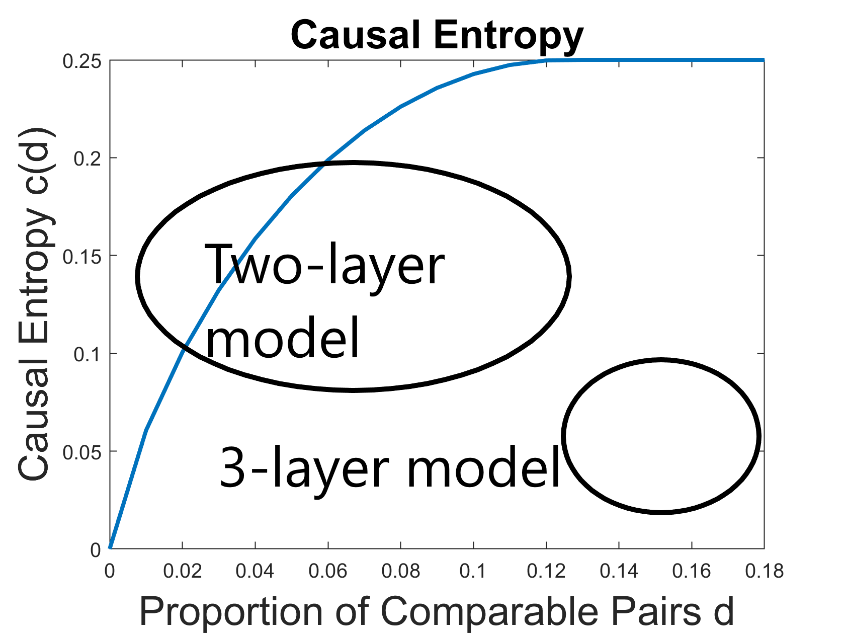
Figure 3: (Left) (Kleitman and Rothschild, 2001) showed that all posets on $n$ variables, as $n\rightarrow\infty$, are asymptotically dominated by the subclass of 3-layer posets, comprised of 3 antichains of sizes $|V_{1}|=|V_{3}|=O(\frac{n}{4}),|V_{2}|=O(\frac{n}{2})$ (see Definition 11). (Right) (Dhar, 1978) investigated poset models parameterized by $dn^{2}$ edges, and discovered phase transitions in their evolution over $d\in(0,\frac{1}{2})$. In the range $0<d\leq\frac{1}{8}$, two layer posets dominate, whereas in the range $\frac{1}{8}\leq d\leq\frac{3}{16}$, three-layer posets are dominant. The plot shows the structural causal entropy function $c(d)$, over $d\in(0,\frac{3}{16}).$

We now define structural causal entropy, based on the parameterization of DAG and poset models using the percentage $d\in(0,1)$ of comparable elements, Remarkably, phase transition effects emerge, as $d$, the proportion of comparable items, is varied (see Figure 3), a result first noted by (Dhar, 1978) connecting statistical physics and the structure of posets.

Definition 12.

Define the space of all causal structures (DAGs or posets) ${\cal P}^{d}_{n}$, where $d\in(0,1)$, such that in any model $P\in{\cal P}^{d}_{n}$, only $dn^{2}$ pairs are comparable. The structural causal entropy of a model $P\in{\cal P}^{d}_{n}$, with $dn^{2}$ comparable relations, where $d\in(0,1)$ is defined as (Dhar, 1978; Prömel et al., 2001a):

$$c(d)=\lim_{n\rightarrow\infty}\frac{\log_{2}|{\cal P}^{d}_{n}|}{n^{2}}$$ (8)

provided the limit exists.

The reason for using the term entropy in this context is that the posets can represent the states of a certain model of a lattice gas with energy proportional to the number of comparable pairs. Given the upper bound given by Equation 7, the following theorem is straightforward to prove.

Theorem 7.

The structural causal entropy of a poset $P\in{\cal P}^{d}_{n}$ on $[n]$ is upper bounded by

$$c(d)\leq\frac{1}{4}$$

Theorem 8.

(Dhar, 1980) (i) The function $\frac{c(d)}{d}$ is a monotonic nonincreasing function of $d$. (ii) The function $\frac{c(d)}{1-d}$ is a monotonic nondecreasing function of $d$.

Remarkably, as $d\in(0,1)$ is varied, (Dhar, 1978) noticed interesting phase transition effects occur, which we will explore below. In particular, (Dhar, 1978) was able to show that in the range $\frac{1}{8}\leq d\leq\frac{3}{16}$, the structural causal entropy $c(d)=\frac{1}{4}$. It is worth understanding this result in more depth.

Theorem 9.

For $d$ in the range $\frac{1}{8}\leq d\leq\frac{3}{16}$, the causal entropy $c(d)=\frac{1}{4}$.

Proof: Let us define $x=\frac{1}{4}-\sqrt{\frac{3}{16}-d}$. Then, as $\frac{1}{8}\leq d\leq\frac{3}{16}$, it must be the case that $0\leq x\leq\frac{1}{4}$. To show the theorem, we have to can construct a DAG of $3$ layers, with $[n]=V_{1}\sqcup V_{2}\sqcup X_{3}$, where $|V_{1}|=(\frac{1}{2}-x)n$ elements, $|V_{2}|=\frac{1}{2}n$ elements, and $|V_{3}|=xn$ elements. For the edges across the layers, insert $\frac{1}{2}|V_{i}||V_{i+1}|$ edges between layers $L_{i}$ and $L_{i+1}$, for $i=1,2$, and all possible edges between $L_{1}$ and $L_{3}$. This can be shown to give a total of $dn^{2}$ relations, hence this DAG will achieve the entropy $c(d)=\frac{1}{4}$ as $n\rightarrow\infty$. ∎

Theorem 10.

The structural entropy of a model $P\in{\cal P}^{d}_{n}$ on $[n]$ for any value of $d\in(0,1)$ in the following ranges is given by:

• $0<d\leq\frac{1}{8}$: In this range for $d$, $c(d)=\frac{1}{4}{\cal H}(4d)$, where ${\cal H}(x)=-x\log_{2}x-(1-x)\log_{2}(1-x)$, the entropy function.

• $\frac{1}{8}\leq d\leq\frac{3}{16}$: In this range for $d$, $c(d)=\frac{1}{4}$, the entropy is constant (as shown in Theorem 9).

Figure 3 plots the value of the causal entropy $c(d)$ over the range $0\leq d\leq\frac{3}{16}$. A phase transition occurs between the ranges $0<d\leq\frac{1}{8}$, when a two-layer poset dominates the space asymptotically, and the range $\frac{1}{8}\leq d\frac{3}{16}$, when as shown by Theorem 9, a three-layer poset architecture dominates the space ${\cal P}^{d}_{n}$.

4 Algorithms for Designing and Testing Multi-partite Causal Designs

We now use the above information-theoretic framework to generalize recent studies of causal inference on large datasets that use bipartite experiments (Li et al., 2020; Pouget-Abadie et al., 2019; Schlosser and Boissier, 2018; Schlosser et al., 2018; Rödder et al., 2019; Charles et al., 2010). Bipartite experiments are characterized by two types of units, interventional units ${\cal T}=\{p_{1},\ldots,p_{k}\}$, – for example, power plants, teachers, items in a marketplace, and neighborhoods – and outcome units ${\cal O}=\{o_{1},\ldots,o_{m}\}$, such as health outcomes of people living near power plants, students in a classroom, prospective buyers in an online marketplace, and residents of a neighborhood.

Definition 13.

Average causal influence $ACI^{\phi}(S)$ of a set of edges $S\subset E_{n}$ in a bipartite DAG $G_{n}=(V_{1}\sqcup V_{2},E_{n})$, where the set of all nodes is partitioned into two disjoint subsets (antichains) $V_{1}$ and $V_{2}$, where $V_{1}$ are the interventional units and $V_{2}$ are the outcome units.

• For $\phi(t)=t\log t$, we get

  $$ACI^{KL}(S,2)=\frac{1}{|S|}\sum_{X_{i}\in\mbox{trg}(S\cap V_{2})}D_{KL}(P(X_{i}|PA_{i})\parallel P_{S}(X_{i}\parallel\mbox{PA}_{i})$$ (9)

  where $S_{i}\in\mbox{trg}(S\cap V_{2})$ is the set of outcome nodes in layer 2 that are in $S$.

• For $\phi(t)=\frac{1}{2}|t-1|$, or $\phi(t)=\frac{1}{2}(\sqrt{t}-1)^{2}$, the resulting decomposition of average causal influence is:

  $${\cal C}^{\phi}_{S}=D_{\phi}(P\parallel P_{S})\leq\sum_{X_{i}\in\mbox{trg}(S\cap V_{2})}D_{\phi}(P_{X_{i}\cup\mbox{Pa}_{i}}\parallel P_{X_{i}\cup\mbox{Pa}^{\bar{S}}_{i}})$$ (10)

where $P$ is the original pre-intervention distribution and $P_{S}$ is the post-intervention distribution.

4.1 Structural Entropy of Multi-partite designs

The two-layer poset architecture in bipartite design can be explained in terms of our structural entropy framework by estimating the empirical value of the number of comparable relations $d$ in these domains. For example, (Harshaw et al., 2021), (McAuley et al., 2015) and others study online experimentation on a large Amazon dataset, where there are over $83$ million reviews made by $121,000$ thousand reviewers on $9.8$ million items. Out of the total set of possible comparable pairs (item reviewer combinations), which would be $9.8x10^{6}\times 121,000$ = $1.1858x10^{12}$ possible comparable pairs,this dataset has only $83$ million comparable items, which translates to the value of $d=\frac{83\times 10^{6}}{9.8\times 10^{6}\times 121,000}\approx\frac{1}{100,000}=10^{-5}$. Since $d$ is close to $0$, the theory confirms that bipartite structures are appropriate. At the threshold point of $d>\frac{1}{8}$, it may be more appropriate to use a tri-partite design, and furthermore, as $d>\frac{3}{16}$, more than $3$ levels may be desirable. To generalize bipartite designs, we note any causal model in ${\cal P}^{d}_{n}$ can be well approximated by a $k$-layer model in ${\cal Q}^{d}_{n}$ (Prömel et al., 2001b). The proof uses Szemerëdi’s regularity lemma (Szemerëdi, 1975).

Definition 14.

The parameterized subclass of $k$-layer poset models ${\cal Q}^{d}_{n}=(\lambda_{1},\ldots,\lambda_{k},p)$ is defined as one where the variables are partitioned into $X=V_{1}\sqcup\ldots V_{k}$ antichains, with $p|V_{i}||V_{i+1}|$ comparable pairs across layers $i,i+1$, $|V_{i}|=\lambda_{i}n$, and $\sum_{i=1}^{n}\lambda_{i}=1$.

Theorem 11.

(Taraz, 1999) For every $\epsilon>0$, and every $0<d<\frac{1}{2}$, there exists constants $k_{0},n_{0}$ such that, for every poset $P\in{\cal P}^{d}_{n}$ with $n\geq n_{0}$, there exists a $k$-partitionable poset $P^{\prime}\in{\cal Q}^{d}_{n}$ with $k\leq k_{0}$ that differs from $P$ in atmost $\epsilon n^{2}$ relations, and in which the partition classes differ in size by at most one.

Definition 15.

Average causal influence $ACI^{\phi}(S,k)$ of a set of edges $S\subset E_{n}$ in a $k$-level DAG $G_{n}=(V_{1}\sqcup\ldots V_{k},E_{n})$, where the set of all nodes is partitioned into $k$ disjoint subsets (antichains) is defined as

• For $\phi(t)=t\log t$, we get

  $$ACI^{KL}(S,k)=\frac{1}{|S|}\sum_{j=2}^{k}\sum_{X_{i}\in\mbox{trg}(S\cap V_{j})}D_{KL}(P(X_{i}|PA_{i})\parallel P_{S}(X_{i}\parallel\mbox{PA}_{i})$$ (11)

  where $X_{i}\in\mbox{trg}(S\cap X_{i})$ is the set of outcome nodes in layer 2 that are in the target set of $S$.

• For $\phi(t)=\frac{1}{2}|t-1|$, or $\phi(t)=\frac{1}{2}(\sqrt{t}-1)^{2}$, the resulting decomposition of average causal influence is:

  $$ACI^{\phi}(S,k)=\frac{1}{|S|}D_{\phi}(P\parallel P_{S})\leq\frac{1}{|S|}\sum_{j=2}^{k}\sum_{X_{i}\in\mbox{trg}(S\cap V_{j})}D_{\phi}(P_{X_{i}\cup\mbox{Pa}_{i}}\parallel P_{X_{i}\cup\mbox{Pa}^{\bar{S}}_{i}})$$ (12)

where $P$ is the original pre-intervention distribution and $P_{S}$ is the post-intervention distribution.

Algorithm 1 specifies a procedure to design a $k$-level DAG architecture that maximizes structural causal entropy. This procedure is based on the theory of evolution of posets (Prömel et al., 2001b; Taraz, 1999). Note that the number of $k$-partite designs $|Q^{n}_{d}|$ is bounded by $\sum_{i=1}^{k-1}{\lambda_{i}\lambda_{i+1}n^{2}\choose p\lambda_{i}\lambda_{i+1}n^{2}}$, ignoring the ways in which variables can be assigned to layers, which adds only a $2^{\mathcal{O}(n\log n)}$ that is negligible under the limit $\lim_{n\rightarrow\infty}\frac{\log_{2}|Q^{n}_{d}|}{n^{2}}$.

Input: A dataset ${\cal D}$ on $[n]$ features, where $n\rightarrow\infty$ (meaning $n$ is very large).

Output: A poset $P\in{\cal P}^{d}_{n}$ on $[n]$, with the induced partial ordering $\leq$.

begin

       Estimate edge density $d$ by sampling relations from the dataset ${\cal D}$.

       Solve the optimization problem in Theorem 12 to determine the asymptotically optimal $k$-layer poset architecture $P\in{\cal Q}^{d}_{n}$, where $P=(\lambda_{1},\ldots,\lambda_{k},p)$ specifies the elements at each layer, and the relations among them.

       Return the poset $P$.

end

Algorithm 1 Given a dataset ${\cal D}$ on $[n]$ features, where $n\rightarrow\infty$ (meaning $n$ is very large), determine the optimal $k$-level poset architecture $P\in{\cal P}^{d}_{n}$ on $[n]$.

Theorem 12.

(Taraz, 1999) The maximum entropy $k$-layer poset architecture ${\cal Q}=(\lambda_{1},\ldots,\lambda_{k},p)$ can be found by solving the following optimization problem:

• Choose $k,\lambda_{1},\ldots,\lambda_{k}$ and $p$ such as to maximize $H(p)\sum_{i=1}^{k-1}\lambda_{i}\lambda_{i+1}$,

• subject to $\frac{1}{2}-\frac{1}{2}\sum_{i=1}^{k}\lambda_{i}^{2}-(1-p)\sum_{i=1}^{k-1}\lambda_{i}\lambda_{i+1}=d$

• where $\sum_{i=1}^{k}\lambda_{i}=1,\ \ 0<\lambda_{i}<1,\ \ \frac{1}{2}\leq p\leq 1$.

4.2 Estimating Causal Influence for Multi-partite designs

Lemma 3.

Hellinger Test:(Acharya et al., 2015, 2018; Daskalakis and Pan, 2017). From $\tilde{\mathcal{O}}(D^{\frac{3}{4}}/\epsilon^{2})$ samples of distributions $P$ and $Q$ over the same finite set of size $D$, we can distinguish between $P=Q$ vs. $D_{H^{2}}(P\parallel Q)\geq\epsilon^{2}$ with error probability at most $1/3$. The error probability can be made smaller than $\delta$ with an additional factor of $\mathcal{O}(\log\frac{1}{\delta})$ in sample complexity.

Input: $k$-layer DAG model ${\cal Q}=(\lambda_{1},\ldots,\lambda_{k},p)$ with distribution $P$, and a set of edges $S$, and threshold $\epsilon$.

Output: Test if causal influence $C^{\phi}(S)\geq\epsilon$.

begin

       For each of $\omega=|V_{k}\cap S|$ outcome nodes, run a squared Hellinger test, where $d$ is the maximum number of parents of any outcome node at layer $k$, $|\Sigma|$ is the size of the discrete alphabet.

       for variable $X_{i}\in S\cap V_{k}$ at layer $k$ do

             Run the Hellinger test to distinguish between

• $H_{0}$: $P_{X_{i}\cup\mbox{Pa}_{i}}=P_{X_{i}\cup\mbox{Pa}^{\bar{S}}_{i}}$

• $H_{1}$: $D_{\phi}(P_{X_{i}\cup\mbox{Pa}_{i}}\parallel P_{X_{i}\cup\mbox{Pa}^{\bar{S}}_{i}})\geq\frac{\epsilon^{2}}{2\omega}$

       end for

      

      If the null hypothesis $H_{0}$ succeeds in all tests, return failure, else return success.

end

Algorithm 2 Given a $k$-layer DAG ${\cal Q}=(\lambda_{1},\ldots,\lambda_{k},p)$ with a distribution $P$, and a set of edges $S$, test whether the causal influence $C^{\phi}(S)\geq\epsilon$.

Theorem 13.

Algorithm 2 computes the causal influence $C^{\phi}(S)$ of a set of edges $S$ in a $k$-partite design (see Definition 15), where $\phi(t)=\frac{1}{2}(\sqrt{t}-1)^{2}$ in time $\tilde{\mathcal{O}}(\frac{|\Sigma|^{\frac{3}{4}(d+1)}\omega}{\epsilon^{2}})$, where $\omega=|S\cap V_{k}|$, by running $\omega$ squared Hellinger tests, where $d$ is the maximum number of parents of any outcome node at layer $k$, and $|\Sigma|$ is the size of the discrete alphabet.

Proof: We exploit the subaddivity of the squared Hellinger distance. We assume a $k$-partite design where all $|V_{k}|=\lambda_{k}n$ outcome units are placed at the bottom $k$th layer, thus we only need to test $\omega=S\cap|V_{k}|$ of them to determine the causal influence. Let $p_{1},\ldots,p_{\omega}$ denote the marginals over the outcome units without intervention, and $q_{1},\ldots,q_{\omega}$ denote the corresponding marginals under intervention on the edges in $S$. Then, if the causal influence of the edges $S$ $D_{H^{2}}(p,q)\geq\epsilon$, subadditivity implies that $\sum_{i=1}^{\omega}\frac{(p_{i}-q_{i})^{2}}{q_{i}}\geq\frac{\epsilon^{2}}{2}$, which is the $\chi^{2}$ divergence over the corresponding vectors $p$ and $q$, and the results from (Acharya et al., 2015) can be used. ∎

We can adapt Algorithm 2 to test for location differences (e.g., shift of the means) in the original and intervened distributions by computing the (sample) expectations, and checking the average treatment effect of the intervention. We can also extend Algorithm 2 to the continuous case, using a linear structural equation model (SEM) to model the outcome of each unit at layer $k$ given a particular exposure to treatment units. In this SEM case, we can view outcomes as a multivariate Gaussian, and we can compare the resulting multivariate Gaussian distributions using the squared Hellinger distance $D_{H^{2}}(P\parallel P_{S})$ for which a closed form expression is well-known.

5 Power-Divergence based Hypothesis Testing of Causal Influence

In this paper, we defined semantic causal entropy as the $\phi$-divergence (Ali and Silvey, 1966; CSISZÁR, 1967) between the original distribution $P$ and the intervention distribution $P_{S}$ over a causal model ${\cal G}=(V,E,P)$ represented as a directed acyclic graph (DAG), where $S\subset E$ is a subset of directed edges whose causal influence is to determined, and $P$ is a probability distribution that is Markov w.r.t. to the conditional independences in the graphical model. We proposed a way to estimate causal influence given a set of samples from both the original distribution $P$ and the intervened distribution $P_{S}$, building on the $\chi^{2}$-based Bayes network hypothesis testing paradigm proposed by (Acharya et al., 2018). Here, we show how to generalize this approach using power-divergence statistics. We can view goodness-of-fit hypothesis tests for a multinomial distribution as testing a hypothesis about the parameters $P=(\pi_{1},\ldots,\pi_{n})$, where each $\pi_{i}$ represents the probability of the $i$-th cell in the multinomial distribution. It is common to define the null hypothesis $H_{0}:\Pi=\Pi_{0}$ where $\Pi_{0}=(\pi_{01},\ldots,\pi_{0n})$ is a pre-specified probability vector. The most widely-used test is Pearson’s $\chi^{2}$ test, which gives the test statistic, given a IID sample of size $m$:

$$X^{2}=\sum_{i=1}^{n}\frac{(X_{i}-m\pi_{0i})^{2}}{m\pi_{0i}}$$ (13)

which is known to asymptotically have a $\chi^{2}$-distribution with $n-1$ degrees of freedom under $H_{0}$, and rejection of the hypothesis occurs when the observed value for $\chi^{2}$ is greater than equal to the pre-specified value found in the $\chi^{2}_{n-1}$ tables.

We now describe a more general paradigm for hypothesis testing for Bayes networks over multinomial distributions, using the power divergence goodness-of-fit tests proposed by (Cressie and Read, 1984). Under the assumption of sub-additivity, which holds for many $\phi$-divergences that satisfy an $\epsilon$-closeness property (Ding et al., 2021), we can use power divergence hypothesis tests as a more flexible and general paradigm than $\chi^{2}$-based tests for measuring causal influences. First, we introduce a directed divergence measure introduced by (Rathie and Kannappan, 1972) that is closely related to the power divergence test proposed by (Cressie and Read, 1984).

Definition 16.

Given two discrete probability distributions $p=(p_{1},\ldots,p_{n})$ and $q=(q_{1},\ldots,q_{n})$, the directed divergence of type $\beta$ is defined as:

$$I^{\beta}_{n}(p\parallel q)=\frac{1}{2^{\beta-1}}\left(\sum_{i=1}^{n}p_{i}^{\beta}q_{i}^{1-\beta}-1\right),\ \ \mbox{for}\ \ \beta\neq 1$$ (14)

It can be easily shown that the directed divergence reduces to KL-divergence in the limit as $\beta$ tends to $1$, that is, $\lim_{\beta\rightarrow 1}I^{\beta}_{n}(p\parallel q)=KL(p\parallel q)$. We now introduce the power divergence between two discrete distributions $p$ and $q$ as follows (Cressie and Read, 1984):

Definition 17.

The power divergence is defined as:

$$I^{\lambda}(p\parallel q)=\frac{1}{\lambda(\lambda+1)}\sum_{i=1}^{n}p_{i}\left[\left(\frac{p_{i}}{q_{i}}\right)^{\lambda}-1\right],\ \ \ -\infty<\lambda<\infty$$ (15)

Since Equation 15 is not defined for $\lambda=-1$ or $\lambda=0$, for these two special cases, it is customary to define power divergences as the continuous limit as $\lim_{\lambda\rightarrow-1}$ and $\lim_{\lambda\rightarrow 0}$, respectively. Table 15 shows how many common goodness-of-fit statistics emerge as special cases of the power divergence test.

Name	$\lambda$ value
$\chi^{2}$-test	$\lambda=1$
Neyman-modified $\chi^{2}$-test	$\lambda=-2$
Loglikelihood ratio statistic	$\lambda=-1$
Freeman-Tukey statistic	$\lambda=-\frac{1}{2}$

Table 1: Power Divergence Test generalizes many common hypothesis tests.

The directed divergence specified by Equation 14 and the power divergence measure specified by Equation 15 are related by the following identity (Cressie and Read, 1984):

$$I^{\lambda}(p\parallel q)=\frac{2^{\lambda}-1}{\lambda(\lambda+1)}I^{\beta+1}(p\parallel q),\ \ \ \lambda\neq-1$$ (16)

Given the original distribution $P=(p_{1},\ldots,p_{n})$ and the intervened distribution $P_{S}=(p^{S}_{1},\ldots,p^{S}_{n})$, we can formally define the power-divergence statistic for measuring causal influence as:

Definition 18.

Given a causal model ${\cal M}=({\cal G},P)$, where $P$ is a multinomial distribution over $n$ variables $X_{1},\ldots,X_{n}$, and $G=(V,E)$ is a DAG, the causal influence of intervening on a set of edges $S\subset E$ is defined by the power-divergence statistic as:

$$D_{\lambda}(P\parallel P_{S})=\frac{1}{\lambda(\lambda+1)}\sum_{i=1}^{n}p_{i}\left[\left(\frac{p_{i}}{p^{S}_{i}}\right)^{\lambda}-1\right],\ \ \ -\infty<\lambda<\infty$$ (17)

where as before, the special cases of $\lambda=-1$ and $\lambda=0$ are treated using appropriate limits. We can show that the power divergence statistic is a special case of the $\phi$-divergence based causal influence model proposed in the paper by specifying the $\phi$ function as follows:

Definition 19.

The power-divergence statistic $D_{\lambda}(P\parallel P_{S})$ is a special case of the $\phi$-divergence based causal influence model $D_{\phi}(P\parallel P_{S})$, if we define $\phi$ as follows:

$$\phi(t)=\frac{t^{\lambda+1}-t-\lambda(t-1)}{\lambda(\lambda+1)},\ \ \ \lambda\neq 0,-1$$ (18)

Finally, we use the results shown by (Ding et al., 2021) on sub-additivity of general $\phi$-divergences when the distributions $P$ and $P_{S}$ are “close" to each other.

Definition 20.

We define the original distribution $P$ on a causal model ${\cal M}=(G,P)$, where $G=(V,E)$ is a DAG on $n$ discrete variables, as one-sided $epsilon$-close to the intervened distribution $P_{S}$, for some subset $S\subset E$ and $0<\epsilon<1$, if for all $i\in[n],\frac{p_{i}}{p^{S}_{i}}<1+\epsilon$. Furthermore, $P$ and $P_{S}$ are two-sided $\epsilon$-close if $1-\epsilon<\frac{p_{i}}{p^{S}_{i}}<1+\epsilon$.

(Ding et al., 2021) showed that most $\phi$-divergences are subadditive when they are applied to causal interventions that yield one-sided or two-sided $\epsilon$-close changes in the resulting distributions.

Theorem 14.

A $\phi$-divergence whose $\phi(t)$ function is continuous on $(0,\infty)$ and twice differentiable at $t=1$ with $\phi^{``}(0)>0$ satisfies $\alpha$ linear subadditivity when $P$ and $P_{S}$ are two-sided $\epsilon$-close with $\epsilon(\alpha)>0$ where $\epsilon(\alpha)$ is a non-increasing function and $\lim_{\alpha\rightarrow 0}=1$, where $\alpha$-linear subadditivity is defined as:

$$D_{\phi}(P\parallel P_{S})-\epsilon\leq\alpha\sum_{X_{i}\in\mbox{trg}(S)}D_{\phi}(P_{X_{i}\cup\mbox{Pa}_{i}}\parallel P_{X_{i}\cup\mbox{Pa}^{\bar{S}}_{i}})$$ (19)

where as before, given a set of intervened edges $S$, the target of intervention is $\mbox{trg}(S)=\{X_{i}|(X_{j},X_{i})\in S\}$. The proof of the above theorem follows directly from the corresponding result in (Ding et al., 2021). This theorem generalizes the causal influence decomposability for $\phi$-divergences given previously, assuming the interventions produce $\epsilon$-close changes.

6 Causal Entropy of Structural Equation Models

Thus far, we have limited the discussion to discrete multinomial models. We extend the scope of causal entropy to linear structural equation models (SEMs) in this section, generalizing the treatment of SEMs developed in (Janzing et al., 2013), which was restricted to the specific case of KL-divergence. We follow the standard practice of assuming that there exists a total ordering of all variables $X_{i},1\leq n$ in the model such that each endogenous variable $X_{i}$ is a (deterministic) function of some subset of variables $X_{j},1\leq j<i$.

Definition 21.

The causal influence ${\cal C}_{X_{i}\rightarrow X_{j}}(P)=D_{KL}(P\parallel P_{X_{i}\rightarrow X_{j}})$ in a structural equation model (SEM) ${\cal M}=(X,\epsilon,f)$ compares the relative entropy between the pre-intervention distribution $P(x_{1},\ldots,x_{n})$, specified by set of deterministic equations $x_{j}=f_{j}(\mbox{pa}_{j},\epsilon_{j})$, where $\{\epsilon_{1},\ldots,\epsilon_{n}\}$ represents a set of jointly independent unobserved noise variables, and the post-intervention distribution $P_{X_{i}\rightarrow X_{j}}$ defined by the modified SEM equations $x_{l}=f_{l}(\mbox{pa}_{l},\epsilon_{l})$, for $l\neq j$, and $x_{j}=f_{j}(\mbox{pa}_{j}\setminus\{x_{j}\},(x^{\prime}_{i},\epsilon_{j}))$.

In effect, intervening on an edge $X_{i}\rightarrow X_{j}$ implies creating an IID copy of $X_{i}$, which is added to that to the noise term in the SEM definition of $X_{j}$. We can write the general SEM equation:

$$X_{j}=\sum_{(i,j)\in E}A_{ij}X_{i}+\epsilon_{j}$$ (20)

where $E$ defines the set of comparable relations in the $k$-partite model (e.g., relations exist between layers, and not within layers). In vector form, we can write the SEM equation as:

$$X=AX+\epsilon,\ \ \ \mbox{or, equivalently}\ \ X=(I-A)^{-1}\epsilon$$ (21)

where $A$ is a strictly lower triangular matrix with zero diagonals, and as before, the $\epsilon$ noise variables are jointly independent. In fact, $A$ is a block diagonal strictly lower triangular matrix to account for the $k$-partitioned structure. The covariance matrix of $X$ can be written as

$$\Sigma=(I-A)^{-1}\Sigma_{\epsilon}(I-A)^{-T}$$ (22)

where $\Sigma_{\epsilon}$ is the covariance matrix of the noise variables $\epsilon$. Consider now an intervention on a subset $S$ of relations in the model, which we represent by decomposing $A=A_{S}+A_{\bar{S}}$, where $A_{S}$ comprises of relations in $S$ and $A_{\bar{S}}$ are those that are not in $S$. The modified SEM equations for the intervened system can be written as follows:

$$X=A_{\bar{S}}X+\epsilon^{\prime},\ \mbox{where}\ \epsilon^{\prime}=\epsilon+A_{S}X^{\prime}$$ (23)

where $X^{\prime}=(X_{1},\ldots,X_{n})$ is an IID copy of $X$, namely $X^{\prime}_{j}$ is distributed like $X_{j}$, and all the variables $X^{\prime},\epsilon$ are jointly independent. The covariance of the modified $\epsilon^{\prime}$, and the intervened system $\Sigma_{S}$ is defined as:

$$\Sigma_{\epsilon^{\prime}}=\Sigma_{\epsilon}+A_{S}\Sigma^{D}_{X}A^{T}_{S},\ \ \Sigma_{S}=(I-A_{S})^{-1}\Sigma_{E}(I-A_{S})^{-T}$$ (24)

Assuming the noise variables $\epsilon$ are jointly independent, we can represent causal influence in terms of the $\phi$-divergence between two multivariate Gaussian distributions, where each distribution can be written as:

$$P(x|\mu,\Sigma)=\frac{1}{\sqrt{(2\pi)^{d}|\Sigma|}}\exp{-\frac{1}{2}(x-\mu)^{T}\Sigma^{-1}(x-\mu)}$$ (25)

where $|\Sigma|$ denotes the determinant of the covariance matrix $\Sigma$, and $d$ is the dimension. The squared Hellinger distance $D_{H^{2}}(P\parallel P_{S})$ between the original distribution $P$ and the intervention distribution $P_{S}$, where $S\subset E$ is the set of edges intervened on, can be written as:

$$D_{H^{2}}(P\parallel P_{S})=1-\frac{|\Sigma|^{\frac{1}{4}}|\Sigma_{S}|^{\frac{1}{4}}}{|\bar{\Sigma}|}\exp\{-\frac{1}{8}(\mu-\mu_{S})^{T}\bar{\Sigma}^{-1}(\mu-\mu_{S})\}$$ (26)

where $\bar{\Sigma}=\frac{\Sigma+\Sigma_{S}}{2}$. Similarly, the KL-divergence $D_{KL}(P\parallel P_{S})$ between the original and intervened distribution is given as:

$$D_{KL}(P\parallel P_{S})=\frac{1}{2}\left(\log\frac{|\Sigma_{S}|}{|\Sigma|}-d+\mbox{Tr}(\Sigma^{-1}_{S}\Sigma)+(\mu-\mu_{S})^{T}\Sigma^{-1}_{S}(\mu-\mu_{S})\right)$$ (27)

If we assume that the variables $X_{i}$ are normalized so that they are mean $0$, then the causal influences simply as shown below, for the above two cases:

$$D_{H^{2}}(P\parallel P_{S})=1-\frac{|\Sigma|^{\frac{1}{4}}|\Sigma_{S}|^{\frac{1}{4}}}{|\bar{\Sigma}|}$$ (28)

$$D_{KL}(P\parallel P_{S})=\frac{1}{2}\left(\log\frac{|\Sigma_{S}|}{|\Sigma|}-d+\mbox{Tr}(\Sigma^{-1}_{S}\Sigma)\right)$$ (29)

Finally, we can define the causal influence in $k$-partite SEM design, using the above definitions, again simplified for the mean $0$ centered case as:

Definition 22.

The $k$-partite average causal influence $ACI^{H^{2}}(S,k)$ using squared Hellinger distance decomposes along each level:

$$ACI^{H^{2}}(S,k)=\frac{1}{|S|}\sum_{j=2}^{k}\sum_{i=1}^{|X_{i}|}{\cal C}_{S^{j}_{i}}(P)=\sum_{j=2}^{k}\sum_{i=1}^{|X_{i}|}\left(1-\frac{|\Sigma|^{\frac{1}{4}}|\Sigma_{S^{j}_{i}}|^{\frac{1}{4}}}{|\bar{\Sigma}|}\right)$$ (30)

where $\bar{\Sigma}=\frac{\Sigma+\Sigma_{S^{J}_{i}}}{2}$.

Definition 23.

The $k$-partite average causal influence using KL-divergence $ACI^{KL}(S,k)$ decomposes along each level:

$$ACI^{KL}(S,k)=\frac{1}{|S|}\sum_{j=2}^{k}\sum_{i=1}^{|X_{i}|}{\cal C}_{S^{j}_{i}}(P)=\sum_{j=2}^{k}\sum_{i=1}^{|X_{i}|}\frac{1}{2}\left(\operatorname{Tr}(\Sigma^{-1}_{S^{j}_{i}}\Sigma)-\log\frac{\det\Sigma}{\det\Sigma_{S^{j}_{i}}}-d\right)$$ (31)

7 Measuring Average Treatment Effect using Run Estimators

The fundamental problem in any causal experiment is to measure the effect of interventions. In bipartite design problems, such as estimating the effect of interventions on power plants on the cardiovascular health outcomes of the residents in nearby locations (Zigler and Papadogeorgou, 2018), the challenge is to design a suitable average treatment effect estimator. In this section, we introduce a new ATE estimator based on the classic Wald Wolfowitz estimator based on run statistics (Noether, 1950), which we define as the WW-ATE estimator. The advantage of our WW-ATE estimator for bipartite experiments, compared to previous estimators, such as correlational clustering (Pouget-Abadie et al., 2019) or its recently proposed generalization, the exposure reweighted linear (ERL) estimator (Harshaw et al., 2021), is that it does not assume knowledge of the interference topology or assume linearity of the exposure or response functions.

We give an intuitive characterization of WW-ATE run statistics estimator, before giving the formal definition of the WW-ATE estimator. Let us take the example of the exposure of residents to pollution from nearby power plants studied by (Zigler and Papadogeorgou, 2018). Let us assume that the outcome units, i.e. residents, have real-valued health outcomes $Y_{1}({\bf z}),Y_{2}({\bf z}),\ldots,Y_{n}({\bf z})$ in response to a particular treatment ${\bf z}$, namely interventions on nearby power plants by implementing some pollution control devices. In measuring average treatment effect, we want to compare the $n$ outcomes under one treatment ${\bf z_{i}}$ with the $n$ outcomes under a different treatment ${\bf z_{j}}$. We assume in this case that the potential outcome functions and exposure functions are monotonic functions of the treatment vectors, which generalizes the linear exposure-response model proposed in (Harshaw et al., 2021), where it is assumed both of these functions are linear. Each pair of interventions ${\bf z}_{i}$ and ${\bf z}_{j}$ yield a sequence of $2n$ potential outcomes:

$$r_{ij}=(Y_{1}({\bf z}_{i}),\ldots,Y_{n}({\bf z}_{i}),Y_{1}({\bf z}_{j}),\ldots,Y_{n}({\bf z}_{j}))$$

Here, $r_{ij}$ is the run sample of potential outcomes based on the pair of tests ${\bf z}_{i}$ and ${\bf z}_{j}$, whose difference we seek to determine. For example, (Harshaw et al., 2021) propose comparing the ATE between the test where all intervention units are treated, namely ${\bf z}_{i}=(+1,\ldots,+1)$, vs the test where none of the intervention units are treated, namely ${\bf z}_{j}=(-1,\ldots,-1)$. Let $r^{s}_{ij}$ be the sorted sequence of potential outcomes in descending order:

$$r^{s}_{ij}=(Y_{p_{1}}({\bf z}_{u_{1}}),\ldots,Y_{p_{2n}}({\bf z}_{u_{2n}})$$

where $u_{k}\in\{i,j\}$ and $Y_{p_{l}}>Y_{p_{l+1}},1\leq l<2n$. Intuitively, the idea behind the WW-ATE estimator is that if the intervention, e.g. pollution control at a power plant, is effective, the health outcomes measured for all nearby residents under the intervention should be higher than the health outcomes measured under no intervention. That is, all the potential outcomes $Y_{1}({\bf z}_{i}),\ldots,Y_{n}({\bf z}_{i})$ should be larger than their corresponding values under no intervention, namely $Y_{1}({\bf z}_{j}),\ldots,Y_{n}({\bf z}_{j})$. If the ordered sequence looks completely random with respect to whether an outcome unit was responding to intervention $i$ or $j$, then the causal effect of the intervention is not measurable.

For each sorted run $r^{s}_{ij}$, define the symbol sequence $s_{ij}$ as

$$s_{ij}=(s^{1}_{ij},\ldots,s^{2n}_{ij})$$

where each symbol $s^{l}_{ij}\in\{+1,-1\}$, where $s^{l}_{ij}=+1$ if the corresponding potential outcome in the $l$th spot in the ordered sequence represents the potential outcome under intervention $i$, and $s^{l}_{ij}=+1$ if the $l$th spot represents the potential outcome under control $j$. What WW-ATE measures is the run statistic, namely the number of contigous sequences of $+1$’s or $-1$’s to decide if the sequence is occurring randomly, or if there is an underlying pattern to the ordering that cannot be explained by chance.

Definition 24.

The Wald-Wolfowitz Average Treatment Effect Run Test (WW-ATE) is defined over two sequences of real-valued observations $X_{1},\ldots,X_{n}$ and $Y_{1},\ldots,Y_{n}$ (representing the potential outcomes under treatment and control). It is assumed that the two sequences are generated independendently.

• The null hypothesis $H_{0}$: the two sequences $X_{i}$ and $Y_{i}$ come from identical distributions.

• The alternate hypothesis $H_{1}$: The two sequences $X_{i}$ and $Y_{i}$ come from different distributions.

• The WW-ATE test statistic is based on computing the number of runs $r$, after pooling the sequences into one sequence of length $2n$ and sorting the sequence in numerically descending order, and converting it to its symbol sequence. A run is a sequence of identical symbols (e.g., +1’s or -1’s).

• The run test statistic $r$ can be shown to be asymptotically normally distributed, and hence its large sample test statistic is given by

  $$z=\frac{(r-\mathbb{E}(r))}{\mbox{Var}(r)}$$ (32)

• The expected value and variance of $r$ is given by:

  $$\mathbb{E}(r)=\frac{2uv}{v+v}+1,\ \ \ \ \mbox{Var(r)}=\frac{2uv(2uv-v-u))}{(v+u)^{2}(u+v-1)}$$ (33)

  where $u$ is the number of $+1$’s in the symbol sequence and $v$ is the number of $-1$’s in the symbol sequence.

• To determine whether the null hypothesis $H_{0}$ should be rejected, and hence the intervention is causally identifiable, since the test statistic $z$ is asymptotically normal, we can compare its value with the standard Normal distribution for significance for a particular $p$-value.

For comparison, the estimator proposed in (Harshaw et al., 2021) for bipartite experiments is given as, where $Y_{i}({\bf z})$ and $x_{i}({\bf z})$ is the potential outcome and exposure of unit $i$ under treatment ${\bf z}$:

Definition 25.

The exposure reweighted linear (ERL) estimator (Harshaw et al., 2021) of the average treatment effect is given as:

$$\hat{\tau}=\frac{2}{n}\sum_{i=1}^{n}Y_{i}({\bf z})\left(\frac{x_{i}({\bf z})-\mathbb{E}[x_{i}({\bf z})]}{\mbox{Var}(x_{i}({\bf z}))}\right)$$ (34)

A detailed experimental study of the run estimator is being planned as part of our future work, which will give deeper insight into its efficacy for bipartite experiments, and its generalization to $k$-partite experiments.

References

- Acharya et al. (2015) Jayadev Acharya, Constantinos Daskalakis, and Gautam Kamath. Optimal testing for properties of distributions. In Corinna Cortes, Neil D. Lawrence, Daniel D. Lee, Masashi Sugiyama, and Roman Garnett, editors, Advances in Neural Information Processing Systems 28: Annual Conference on Neural Information Processing Systems 2015, December 7-12, 2015, Montreal, Quebec, Canada, pages 3591–3599, 2015. URL https://proceedings.neurips.cc/paper/2015/hash/1f36c15d6a3d18d52e8d493bc8187cb9-Abstract.html.
- Acharya et al. (2018) Jayadev Acharya, Arnab Bhattacharyya, Constantinos Daskalakis, and Saravanan Kandasamy. Learning and testing causal models with interventions. In S. Bengio, H. Wallach, H. Larochelle, K. Grauman, N. Cesa-Bianchi, and R. Garnett, editors, Advances in Neural Information Processing Systems, volume 31. Curran Associates, Inc., 2018. URL https://proceedings.neurips.cc/paper/2018/file/78631a4bb5303be54fa1cfdcb958c00a-Paper.pdf.
- Ali and Silvey (1966) S. M. Ali and S. D. Silvey. A general class of coefficients of divergence of one distribution from another. Journal of the Royal Statistical Society: Series B (Methodological), 28(1):131–142, 1966. doi:https://doi.org/10.1111/j.2517-6161.1966.tb00626.x. URL https://rss.onlinelibrary.wiley.com/doi/abs/10.1111/j.2517-6161.1966.tb00626.x.
- Ay and Polani (2008) Nihat Ay and Daniel Polani. Information flows in causal networks. Adv. Complex Syst., 11(1):17–41, 2008. doi:10.1142/S0219525908001465. URL https://doi.org/10.1142/S0219525908001465.
- Bailey et al. (2007) Delbert D. Bailey, Víctor Dalmau, and Phokion G. Kolaitis. Phase transitions of pp-complete satisfiability problems. Discret. Appl. Math., 155(12):1627–1639, 2007. doi:10.1016/j.dam.2006.09.014. URL https://doi.org/10.1016/j.dam.2006.09.014.
- Brinkmann and McKay (2002) Gunnar Brinkmann and Brendan D. McKay. Posets on up to 16 points. Order, 19:147–179, 2002.
- Charles et al. (2010) Denis Xavier Charles, Max Chickering, Nikhil R. Devanur, Kamal Jain, and Manan Sanghi. Fast algorithms for finding matchings in lopsided bipartite graphs with applications to display ads. In David C. Parkes, Chrysanthos Dellarocas, and Moshe Tennenholtz, editors, Proceedings 11th ACM Conference on Electronic Commerce (EC-2010), Cambridge, Massachusetts, USA, June 7-11, 2010, pages 121–128. ACM, 2010. doi:10.1145/1807342.1807362. URL https://doi.org/10.1145/1807342.1807362.
- Cressie and Read (1984) Noel Cressie and Timothy R. C. Read. Multinomial goodness-of-fit tests. Journal of the Royal Statistical Society. Series B (Methodological), 46(3):440–464, 1984. ISSN 00359246. URL http://www.jstor.org/stable/2345686.
- CSISZÁR (1967) I. CSISZÁR. Information-type measures of difference of probability distributions and indirect observation. Studia Scientiarum Mathematicarum Hungarica, 2:229–318, 1967. URL https://ci.nii.ac.jp/naid/10028997448/en/.
- Daskalakis and Pan (2017) Constantinos Daskalakis and Qinxuan Pan. Square Hellinger subadditivity for Bayesian networks and its applications to identity testing. In Satyen Kale and Ohad Shamir, editors, Proceedings of the 2017 Conference on Learning Theory, volume 65 of Proceedings of Machine Learning Research, pages 697–703. PMLR, 07–10 Jul 2017. URL http://proceedings.mlr.press/v65/daskalakis17a.html.
- Dhar (1978) Deepak Dhar. Entropy and phase transitions in partially ordered sets. Journal of Mathematical Physics, 19(8):1711–1713, 1978.
- Dhar (1980) Deepak Dhar. Asymptotic enumeration of partially ordered sets. Pacific Journal of Mathematics, 90(2):299–305, 1980.
- Ding et al. (2021) Mucong Ding, Constantinos Daskalakis, and Soheil Feizi. Gans with conditional independence graphs: On subadditivity of probability divergences. In Arindam Banerjee and Kenji Fukumizu, editors, The 24th International Conference on Artificial Intelligence and Statistics, AISTATS 2021, April 13-15, 2021, Virtual Event, volume 130 of Proceedings of Machine Learning Research, pages 3709–3717. PMLR, 2021. URL http://proceedings.mlr.press/v130/ding21e.html.
- Eberhardt (2008) Frederick Eberhardt. Almost optimal intervention sets for causal discovery. In David A. McAllester and Petri Myllymäki, editors, UAI 2008, Proceedings of the 24th Conference in Uncertainty in Artificial Intelligence, Helsinki, Finland, July 9-12, 2008, pages 161–168. AUAI Press, 2008. URL https://dslpitt.org/uai/displayArticleDetails.jsp?mmnu=1&smnu=2&article_id=1948&proceeding_id=24.
- Frieze and Tkocz (2020) Alan M. Frieze and Tomasz Tkocz. Random graphs with a fixed maximum degree. SIAM J. Discret. Math., 34(1):53–61, 2020. doi:10.1137/19M1249928. URL https://doi.org/10.1137/19M1249928.
- Harshaw et al. (2021) Christopher Harshaw, David Eisenstat, Vahab Mirrokni, and Jean Pouget-Abadie. Design and analysis of bipartite experiments under a linear exposure-response model. Arxiv, 2021.
- Hauser and Bühlmann (2012) Alain Hauser and Peter Bühlmann. Characterization and greedy learning of interventional markov equivalence classes of directed acyclic graphs. J. Mach. Learn. Res., 13:2409–2464, 2012. URL http://dl.acm.org/citation.cfm?id=2503320.
- Imbens and Rubin (2015) Guido W. Imbens and Donald B. Rubin. Causal Inference for Statistics, Social, and Biomedical Sciences: An Introduction. Cambridge University Press, USA, 2015. ISBN 0521885884.
- Jacot et al. (2018) Arthur Jacot, Clément Hongler, and Franck Gabriel. Neural tangent kernel: Convergence and generalization in neural networks. In Samy Bengio, Hanna M. Wallach, Hugo Larochelle, Kristen Grauman, Nicolò Cesa-Bianchi, and Roman Garnett, editors, Advances in Neural Information Processing Systems 31: Annual Conference on Neural Information Processing Systems 2018, NeurIPS 2018, December 3-8, 2018, Montréal, Canada, pages 8580–8589, 2018. URL https://proceedings.neurips.cc/paper/2018/hash/5a4be1fa34e62bb8a6ec6b91d2462f5a-Abstract.html.
- Janzing et al. (2013) Dominik Janzing, David Balduzzi, Moritz Grosse-Wentrup, and Bernhard Scholkopf. Quantifying causal influences. The Annals of Statistics, 41(5):2324 – 2358, 2013. doi:10.1214/13-AOS1145. URL https://doi.org/10.1214/13-AOS1145.