Chaoticity in the vicinity of complex unstable periodic orbits in galactic type potentials

Abstract

We investigate the evolution of phase space close to complex unstable periodic orbits in two galactic type potentials. They represent characteristic morphological types of disc galaxies, namely barred and normal (non-barred) spiral galaxies. These potentials are known for providing building blocks to support observed features such as the peanut, or X-shaped bulge, in the former case and the spiral arms in the latter. We investigate the possibility that these structures are reinforced, apart by regular orbits, also by orbits in the vicinity of complex unstable periodic orbits. We examine the evolution of the phase space structure in the immediate neighbourhood of the periodic orbits in cases where the stability of a family presents a successive transition from stability to complex instability and then to stability again, as energy increases. We find that we have a gradual reshaping of invariant structures close to the transition points and we trace this evolution in both models. We conclude that for time scales significant for the dynamics of galaxies, there are weakly chaotic orbits associated with complex unstable periodic orbits, which should be considered as structure-supporting, since they reinforce the morphological features we study.

1 Introduction

Complex instability is a particular type of orbital instability that appears in autonomous Hamiltonian systems of three or more degrees of freedom (for a definition see Sect. 2). In galactic dynamics it characterizes periodic orbits of many three dimensional (hereafter 3D) models in a large volume of their parameter space (Magnenat, 1982a, b; Pfenniger, 1984, 1985b; Contopoulos and Magnenat, 1985; Contopoulos, 1986; Martinet and Pfenniger, 1987; Pfenniger, 1987; Martinet and de Zeeuw, 1988; Zachilas, 1988; Patsis and Zachilas, 1990; Zachilas, 1993; Patsis and Zachilas, 1994; Olle and Pfenniger, 1998; Katsanikas et al., 2011; Patsis and Katsanikas, 2014). However, considerable insight in the role of complex instability for the dynamics of Hamiltonian systems has been gained by works on several other kinds of potentials (Heggie, 1985; Papadaki et al., 1995; Ollé and Pacha, 1999) or 4-dimensional symplectic mappings (Pfenniger, 1985a; Contopoulos and Giorgilli, 1988; Olle and Pfenniger, 1995; Jorba and Ollé, 2004; Delis and Contopoulos, 2016; Stöber and Bäcker, 2021). These results have also been used for understanding the behaviour of stellar orbits in galactic type potentials.

A main problem in galactic dynamics is to find the orbital building blocks that can reinforce observed morphological features in galaxies. In that respect, finding stable periodic orbits, which attract around them quasi-periodic orbits that remain in their neighbourhood, is essential for understanding the enhancement of bars and spiral arms in 3D autonomous, rotating, Hamiltonian systems representing disc galaxies. Nevertheless, the quasi-periodic orbits must provide the appropriate shapes that match the morphology of the structure we study.

A particular structure can also be supported during a certain time by orbits that remain confined during this period in a specific volume of the phase space. Such orbits are called sticky and have been mainly studied in two-dimensional systems (see Contopoulos and Harsoula, 2010, and references therein). Much less work has been done on stickiness in 3D models and especially in the neighbourhood of complex unstable periodic orbits. The present study investigates whether we can find orbits that remain confined close to periodic orbits characterized by this type of instability.

Complex instability has been considered as an abrupt transition to chaos, since its appearance is not associated with the introduction of new families of periodic orbits in the system. In any case, studies of the phase space in the neighbourhood of complex unstable periodic orbits have shown that the transition from stability to complex instability gives rise to bifurcating invariant structures in Poincaré sections of 3D autonomous Hamiltonian systems (Pfenniger, 1985b; Papadaki et al., 1995; Olle and Pfenniger, 1998; Ollé et al., 2004; Katsanikas et al., 2011), as well as in 4D symplectic maps (Pfenniger, 1985a; Jorba and Ollé, 2004; Zachilas et al., 2013).

A question that arises, is if the degree of chaoticity of orbits close to a complex unstable periodic orbit can be associated with some quantity that can indicate the presence or absence of invariant forms in the corresponding phase space region. From the analysis leading to the stability of the periodic orbits, the obvious candidate is the discriminant $\Delta$ (for the definition see Sect. 2 below). One of the goals of the present paper is to investigate its relation with chaoticity in phase space, as quantified by chaos indicators like the GALI₂ index, introduced by Skokos et al. (2007). However, the ultimate goal of the study is to explore whether or not one can find close to complex unstable periodic orbits building blocks for supporting structures like the two main morphological features of disc galaxies, which are the bars and the spiral arms.

The paper is structured as follows: In Section 2 we present the various kinds of instabilities of periodic orbits in 3D systems. In Section 3 we describe the two dynamical models, which we have used in our study, namely the Ferrers bar and the PERLAS potential. In Section 4 we give definitions associated with the GALI₂ indicator. Our numerical results are presented in Section 5. Finally we enumerate our conclusions in Section 6.

2 Orbital instabilities in 3D systems

In galactic disc dynamics we deal with disc-like potentials, rotating around an axis perpendicular to the disc, at the center of the system. In such a case, our Hamiltonian can be described in Cartesian coordinates $(x,y,z)$ as:

$$H=\frac{1}{2}(p_{x}^{2}+p_{y}^{2}+p_{z}^{2})+V(x,y,z)-\Omega_{s}(xp_{y}-yp_{x}),$$ (1)

where $V(x,y,z)$ is the potential of the model, $\Omega_{s}$ the rotational velocity of the system (pattern speed), which is constant and $p_{x},~{}p_{y},$ and $p_{z}$ are the canonically conjugate momenta. The axis of rotation is the $z$ axis.

We will refer to the conserved numerical value of the Hamiltonian, $E_{J}$, as the Jacobi constant or, more loosely, as the ‘energy’.

The equations of motion corresponding to Eq. 1 are:

$$\dot{x}=p_{x}+\Omega_{s}y, \dot{y}=p_{y}-\Omega_{s}x, \dot{z}=p_{z}$$

$$\dot{p_{x}}=-\frac{\partial V}{\partial x}+\Omega_{s}p_{y}, \displaystyle{\dot{p_{y}}=-\frac{\partial V}{\partial y}-\Omega_{s}p_{x},} \dot{p_{z}}=-\frac{\partial V}{\partial z}.$$ (2)

The space of section in the case of a 3D system is 4D. The equations of motion for a given $E_{J}$ are solved numerically, starting with initial conditions $(x_{0},z_{0},p_{x_{0}},p_{z_{0}})$ in the plane $y$=0 (with the $p_{y_{0}}$ value determined by the given E_J value) and then by considering successive upwards ($p_{y}>0$) intersection with this plane.

The exact initial conditions for the periodic orbit are calculated using a Newton iterative method. A periodic orbit is found when the initial and final coordinates coincide with an accuracy of at least 10^-10. The integration scheme used was a 4th order Runge-Kutta algorithm and in some cases a Runge-Kutta Fehlberg 7-8th order scheme, securing a relative error in the energy less than $10^{-14}$.

Resonances play a crucial role in the dynamics of rotating, 3D, galactic potentials. These are resonances between the epicyclic and the rotational frequencies of the stellar orbits, in the rotating with $\Omega_{s}$ frame of reference (radial resonances), while we have vertical frequencies as well, in which, instead of the epicyclic, we consider the vertical frequency. A special case is the corotation resonance, where the angular velocity of the stars is equal to the pattern speed, namely $\Omega(r)$ = $\Omega_{s}$ (for definitions see e.g. Patsis and Grosbol, 1996). For the needs of the present study we keep in mind that at the resonances the stability of a family of periodic orbits, i.e. of periodic solutions of the equations of motion (2), may change (Contopoulos and Grosbol, 1989).

When a periodic orbit is found, it can be characterized as stable or unstable by calculating its linear stability. This is done by following a method introduced by Broucke (1969) and Hadjidemetriou (1975). Contopoulos and Magnenat (1985) have distinguished three kinds of instability for the unstable periodic orbits. The method is briefly described below, where we also give the definitions of the instabilities.

The first step is to consider a small deviation from the initial conditions of the periodic orbit and then to integrate the perturbed orbit again up to the next upward intersection. In this way a 4D Poincaré map, $T:\mathbf{R}^{4}\to\mathbf{R}^{4}$, is established, relating the points of initial with the final deviation. In vector form this relation can be written as: $\vec{\xi}=M\,\vec{\xi_{0}}$, where $\vec{\xi}$ is the final deviation, $\vec{\xi_{0}}$ is the initial deviation and $M$ a $4\times 4$ matrix, called the monodromy matrix. The characteristic equation of this matrix is written in the form $\lambda^{4}+\alpha\lambda^{3}+\beta\lambda^{2}+\alpha\lambda+1=0$. Its solutions $(\lambda_{i},i=1,2,3,4)$, obey the relations $\lambda_{1}\,\lambda_{2}=1$ and $\lambda_{3}\,\lambda_{4}=1$ and we can write for each pair:

$$\lambda_{i},1/\lambda_{i}=\frac{1}{2}\left[-b_{i}\pm(b_{i}^{2}-4)^{\frac{1}{2}}\right],$$ (3)

where $\displaystyle b_{i}=\frac{1}{2}\,(\alpha\pm\Delta^{1/2})$ and

$$\Delta=\alpha^{2}-4(\beta-2).$$ (4)

Stability or Instability of the periodic orbit is expressed by means of the quantities $b_{1},b_{2}$ and $\Delta$. The quantities $b_{1}$ and $b_{2}$ are called the stability indices. One of them is associated with radial and the other one with vertical perturbations. We distinguish the following four cases:

1. If $\Delta>0$, $|b_{1}|<2$ and $|b_{2}|<2$, the 4 eigenvalues $\lambda_{i}(i=1,2,3,4)$ are on the unit circle and the periodic orbit is called ‘stable’, (S).

2. If $\Delta>0$, and $|b_{1}|>2$, $|b_{2}|<2$, or $|b_{2}|>2$, $|b_{1}|<2$, two eigenvalues are on the real axis and two on the unit circle, and the periodic orbit is called ‘simple unstable’, (U).

3. If $\Delta>0$, $|b_{1}|>2$, and $|b_{2}|>2$, all four eigenvalues are on the real axis, and the periodic orbit is called ‘double unstable’, (DU).

4. Finally, $\Delta<0$ means that all four eigenvalues are complex numbers but off the unit circle. The orbit is characterized then as “complex unstable”, ($\Delta$).

For a general discussion of the kinds of instability encountered in Hamiltonian systems of N degrees of freedom the reader may refer to Skokos (2001).

As one of the parameters of our model varies (in this work $E_{J}$), case (4) may appear at an S$\rightarrow\!\!\Delta$ or at a DU$\rightarrow\!\!\Delta$ transition. When the periodic orbit is initially stable, we have at a critical $E_{J}$, a pairwise collision of eigenvalues on two conjugate points of the unit circle. Then, Krein-Moser theorem (see e.g. Contopoulos, 2002, p.298) decides if the eigenvalues will remain on the unit circle after the collision, or if they will move out of the unit circle, into the complex plane, forming a complex quadruplet. In the former case the orbits of the family will continue being stable and in the latter they will become complex unstable. The transition from stability to complex instability is also known as Hamiltonian Hopf Bifurcation (van der Meer, 1985).

At complex instability, unlike in the two other kinds of instabilities, we do not have introduction of new families of periodic orbits in the system. In the case of a S$\rightarrow$U transition, the stability of the parent family is inherited to a bifurcated one. Thus, for values of the parameter beyond the critical value for which the stability of the family changes, new tori of quasiperiodic orbits will appear in the phase space of the system, belonging to the new stable families. The U$\rightarrow$DU transition occurs to a later stage and can be considered as a transition from order to chaos in two steps (S$\rightarrow$U$\rightarrow$DU). A bifurcated family at the U$\rightarrow$DU transition will be simple unstable. At a DU$\rightarrow\!\!\Delta$ transition no new families are introduced in the system. We note that in the latter case the neighbourhood of the parent family is already chaotic and no new invariant structures are encountered in phase space (Katsanikas et al., 2011).

3 The Dynamical Models

Complex instability appears frequently, as energy varies, in the evolution of the stability of the main 3D families of periodic orbits that bifurcate from the central, planar family of periodic orbits x1, and make up the “x1-tree” (Skokos et al., 2002). The most important of these families is x1v1, which bifurcates from x1, usually as stable (but see also Patsis and Harsoula, 2018), at the vertical 2:1 resonance. The existence of the x1-tree families is not associated with a particular model, but it is an intrinsic property of any 3D rotating potential, in which the resonances can be defined. They offer the building blocks for supporting the main structures encountered in disc galaxies, namely the bar (see e.g. Patsis et al., 2002) and the spirals (Patsis and Grosbol, 1996; Chaves-Velasquez et al., 2019).

3.1 Ferrers bar

The first potential we used, refers to a mass distribution representing a galactic bar. The 3D bar is rotating around its short $z$ axis. The $x$ axis is the intermediate and the $y$ axis the long one. The system is rotating with the pattern speed of the bar $\Omega_{b}$, i.e. $\Omega_{s}=\Omega_{b}$. The bar is embedded in a 3D disc, while in the center of the system exists also a spheroidal bulge. Thus, this galactic model consists of three components, a disc, a bulge and a bar.

The disc is represented by a Miyamoto potential (Miyamoto and Nagai, 1975):

$$\Phi_{D}=-\frac{GM_{D}}{\sqrt{x^{2}+y^{2}+(A+\sqrt{B^{2}+z^{2}})^{2}}},$$ (5)

where $M_{D}$ is the total mass of the disc, $A$ and $B$ are the horizontal and vertical scale lengths, and $G$ is the gravitational constant.

The bulge is modelled by a Plummer sphere with potential:

$$\Phi_{S}=-\frac{GM_{S}}{\sqrt{x^{2}+y^{2}+z^{2}+\epsilon_{s}^{2}}},$$ (6)

where $\epsilon_{s}$ is the scale length of the bulge and $M_{S}$ is its total mass.

The third component of the potential is a triaxial Ferrers bar, whose density $\rho$ is:

$$\rho=\left\{\begin{array}[]{lcc}\displaystyle{\frac{105M_{B}}{32\pi abc}(1-m^{2})^{2}}&{\mbox{f}or}&m\leq 1\\ &&\\ \displaystyle{0}&{\mbox{f}or}&m>1\end{array}\right.,$$ (7)

where

$$m^{2}=\frac{y^{2}}{a^{2}}+\frac{x^{2}}{b^{2}}+\frac{z^{2}}{c^{2}}\,\,,\,\,\,a>b>c,$$ (8)

$a$, $b$, $c$ are the semi-axes and $M_{B}$ is the mass of the bar component. The corresponding potential $\Phi_{B}$ and the forces are given in a closed form in Pfenniger (1984). We use for the Miyamoto disc A=3 and B=1, and for the Ferrers bar axes we set $a\!:\!b\!:\!c$ = $6\!:\!1.5\!:\!0.6$, as in Pfenniger (1984) and in many previous works of the authors using this potential. The masses of the three components satisfy $G(M_{D}+M_{S}+M_{B})=1$. The length unit is taken as 1 kpc, the time unit as 1 Myr and the mass unit as $2\times 10^{11}M_{\odot}$. In Table 1 we give the parameters of our model. They have been chosen so, that for this model we have a typical alternation of stable and complex unstable regions in the x1v1 family, as the energy varies.

Table 1: The parameters of the Ferrers bar model: G is the gravitational constant, M_D, M_B, M_S are the masses of the disc, the bar and the bulge respectively, $\epsilon_{s}$ is the scale length of the bulge, $\Omega_{b}$ is the pattern speed of the bar, $E_{J}$(v-IILR) is the value of the Jacobi constant for the vertical 2:1 resonance and $R_{c}$ is the corotation radius.

GMD	GMB	GMS	$\epsilon_{s}$	$\Omega_{b}$	$E_{J}$(v-ILR)	$R_{c}$
0.87	0.05	0.08	0.4	0.054	-0.3028	6.38

3.2 PERLAS spirals

The second potential we used, refers to a bisymmetric logarithmic spiral as those observed in grand design spiral galaxies. Spirals are, besides the bars, the second feature that characterizes the morphology of disc galaxies. They may appear together with a bar (barred-spiral galaxies) or without a bar (normal spiral galaxies). The spiral potential is embedded in an axisymmetric background that has three parts. The first two parts are represented by the same general models we used for the axisymmetric components of the bar model. Namely, we have first a central mass component, $\Phi_{S}$, representing the bulge, given again by Eq. 6, with mass $M_{S}$ and scale length $\epsilon_{s}$. In addition, we consider a 3D Miyamoto disc (Eq. 5) with mass $M_{D}$ and scale lengths $A$, $B$.

The third component of the axisymmetric part of the spiral potential refers to a massive halo, represented by a halo potential proposed by Allen and Santillan (1991), which at radius $r$ is given by

$$\Phi_{H}(r)=-\left(\frac{M(r)}{r}\right)-\left(\frac{M_{H}}{1.02a_{H}}\right)\times\left[-\frac{1.02}{1+(r/a_{H})^{1.02}}+\ln(1+(r/a_{H})^{1.02})\right]^{100}_{r},$$

where

$$M(r)=\frac{M_{H}(r/a_{H})^{2.02}}{1+(r/a_{H})^{1.02}}.$$ (9)

$M(r)$ has mass units, $M_{H}$ is the mass of the halo, and $a_{H}$ is a scale length.

The perturbation in this case has the form of a three dimensional spiral component, for which we use the PERLAS (sPiral arms potEntial foRmed by obLAte Spheroids) potential (Pichardo et al., 2003). The spiral pattern has two arms and is shaped by a density distribution formed by individual, inhomogeneous, oblate Schmidt spheroids (Schmidt, 1956), These spheroids are superposed along a logarithmic spiral locus of constant pitch angle $i$. The spirals are considered to be trailing and rotating clockwise.

The Schmidt spheroids have constant semi-axes ratio, while their density falls linearly outwards, starting from their centres on the spiral locus. The separation among the centres of the spheroids is 0.5 kpc, their total width 2 kpc and their total height 1 kpc, The spiral arms start at 2.03 kpc and end at 12.9 kpc. These distances correspond to the radial 2:1 resonance and to 1.5 times the corotation radius respectively. The density along the loci of the spiral arms falls exponentially, as the one of the disc does. For a detailed presentation of the PERLAS potential see e.g. Pérez-Villegas et al. (2012).

The total potential is the sum of the four terms: $\Phi=\Phi_{S}+\Phi_{D}+\Phi_{H}+\Phi_{SP}$, the three first of which compose the axisymmetric part and $\Phi_{SP}$ is the PERLAS spiral potential. The parameters for all these components used in the particular model of the present paper are summarized in Table 2.

Table 2: Parameters of the PERLAS potential. The upper row refers to the spiral part, while the two lower rows give the values of all parameters of the axisymmetric components (see text).

Spiral part
Galaxy type	Locus	Arms Number	Pitch Angle $i^{o}$	$\mu=M_{SP}/M_{D}$	Scale length (kpc)	$\Omega_{p}$ ($\text{km}/\text{s}/\text{kpc}$)
Sc	Logarithmic	$2$	$25^{o}$	$0.04$	$3.7$	$-20$
Axisymmetric Components
$M_{D}/M_{H}$	$M_{S}/M_{D}$	Maximum of rotation velocity ($\text{km}\text{s}^{-1}$)	$M_{D}(10^{10}M_{\odot})$	$M_{S}(10^{10}M_{\odot})$	$M_{H}(10^{11}M_{\odot})$	Disc Scale length (kpc)
$0.1$	$0.2$	$170$	$5.10$	$1.02$	$4.85$	$3.7$
	$\epsilon_{s}$ (kpc)	$A$ (kpc)	$B$ (kpc)	$a_{H}$ (kpc)
	1	5.32	0.25	12

The pattern speed $\Omega_{p}=-20$ km s^-1 kpc^-1 defines the angular velocity of the system in the clockwise sense, while the pitch angle of the logarithmic spirals, $i=25^{\circ}$, corresponds to an open pattern, typical of galaxies of galactic type Sc. The model has a maximum rotational velocity of 170 $\text{km}\text{s}^{-1}$, that is typical for a galaxy of morphological type Sc (Rubin et al., 1980). The amplitude of the perturbation is determined by the ratio $M_{SP}/M_{D}$, where $M_{SP}$ is the mass of the spiral and $M_{D}$ the mass of the disc component (Chaves-Velasquez et al., 2019). This set up has been chosen for the needs of the present paper, since the stability of the basic 3D family x1v1, which supports the spiral arms (Chaves-Velasquez et al., 2019), has successive stable and complex unstable parts, as E_J varies. We note that the scaling of units in the two models is not the same, so the numerical values referring to the Ferrers bar and the PERLAS model are different.

4 The GALI₂ indicator

In order to quantify the chaoticity of the orbits we consider in the present study, we use the standard chaos indicator GALI₂ (Skokos et al., 2007).

The GALI₂ index is given by the norm of the wedge product of two normalized to unity deviation vectors $\mathbf{\hat{w}}_{1}(t)$ and $\mathbf{\hat{w}}_{2}(t)$: $\rm{GALI}_{2}(t)=|\mathbf{\hat{w}}_{1}(t)\wedge\mathbf{\hat{w}}_{2}(t)|.$ The initial coordinates of the deviations vectors are chosen randomly, and the two vectors are orthonormalized by using the Gram-Schmidt process at the beginning of the integration. This sets the initial value of the index to $\mbox{GALI}_{2}(0)=1$. Thus, in order to evaluate GALI₂ we integrate the equations of motion and the variational equations for two deviation vectors simultaneously. The GALI₂ index behaves as follows (see Skokos and Manos, 2016, and references therein):

• For chaotic orbits it falls exponentially to zero as: $\mbox{GALI}_{2}(t)\propto\exp{(-(\lambda_{1}-\lambda_{2})t)}$, where $\lambda_{1}$ and $\lambda_{2}$ are the two largest Lyapunov exponents (for definitions and for the computation of the Lyapunov exponents see e.g: Benettin et al., 1980; Skokos, 2010).

• For regular orbits it oscillates around a positive value across the integration: $\mbox{GALI}_{2}(t)\propto constant$.

• In the case of sticky orbits we observe a transition from practically constant GALI₂ values, which correspond to the seemingly quasiperiodic epoch of the orbit, to an exponential decay to zero, which indicates the orbit’s transition to chaoticity.

GALI₂ has been used to characterize the chaoticity of the orbits, both in Ferrers bars (Manos and Athanassoula, 2011) as well as in PERLAS potentials (Chaves-Velasquez et al., 2019).

5 Results

5.1 Complex Unstable regions in Ferrers bars

We have studied the chaoticity in the neighbourhood of complex unstable periodic orbits belonging to the family x1v1 (Skokos et al., 2002) in two energy regions of our Ferrers bars model. The orbits of this family are important, because they act as building blocks for the peanut-shaped bulges in the central regions of barred galaxies (Patsis et al., 2002). In the first case we studied, the complex unstable region is found between a S$\rightarrow\!\!\Delta$ transition at E_J $\approx-0.3028$ and a $\Delta\!\!\rightarrow$S transition at E_J $\approx-0.293$. At the critical E_J values, there is a sign change of $\Delta$, being $\Delta<0$ in the complex unstable region. In Fig. 1 we give the variation of $\Delta$ in the $-0.304\leq E_{J}\leq-0.291$ interval.

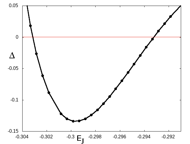
Figure 1: Ferrers bar: The variation of $\Delta$ (Eq. 4) for the x1v1 family of periodic orbits in the $-0.304\leq E_{J}\leq-0.291$ region

. The heavy dots correspond to calculated periodic orbits. Those with $\Delta<0$ are complex unstable.

The quantity $\Delta$ (Eq. 4) refers to the periodic orbit itself. In order to find out whether, and how, it is associated with the phase space structure in the neighbourhood of x1v1, we perturbed the initial conditions of the orbits of this family at different E_J ​. We first investigated orbits with initial conditions those of the periodic orbit, with one of the coordinates perturbed by 10% of its value. We consider this as a reasonable perturbation of a periodic orbit for finding non-periodic orbits that could potentially participate in the reinforcement of the peanut-shaped bulge. In particular, at each E_J ​​, we calculated first the GALI₂ index of an orbit with the initial conditions of x1v1, perturbed in the $x$-direction by $0.1x_{0}(\rm{x1v1})$ and then the GALI₂ index of an orbit with the initial conditions of x1v1 perturbed in the $z$-direction by $0.1z_{0}(\rm{x1v1})$. The evolution of GALI₂ with E_J for orbits in the $-0.3073\leqq E_{J}\leqq-0.2923$ interval is given in Fig. 2. The left column refers to the orbits with the x1v1 initial conditions perturbed in the $x$-direction, while in the right column to the orbits perturbed in the $z$-direction. The E_J of each orbit is given in the lower left corner of the panels.

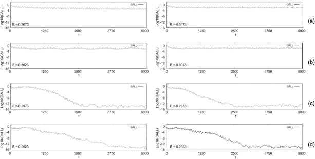
Figure 2: Ferrers bar: The GALI₂ indices of orbits in the first S$\rightarrow\Delta\rightarrow$S transition, for which we have calculated $\Delta$ in Fig. 1. In the left column the orbits have x1v1 initial conditions perturbed in the x-direction by 10% of $x_{0}$, while in the right column the orbits are again x1v1, but perturbed this time in the z-direction by 10% of $z_{0}$ (see text). In (a) and (d) the corresponding periodic orbit is stable (S), while in (b) and (c) complex unstable ($\Delta$). In (d), the perturbed orbit close to a stable x1v1 has a chaotic behaviour. The integration time corresponds to 5 Gyr.

At E_J =$-0.3073$, the representative of x1v1 is stable and the perturbed by 10% in the $x$- and $z$-directions nearby orbits (left and right panels in Fig. 2a) are regular, apparently belonging to a quasiperiodic orbit trapped around it. The orbits in Fig. 2b are at an E_J just beyond the S$\rightarrow\!\!\Delta$ transition, namely E_J =$-0.3023$, where x1v1 is already complex unstable. However, GALI₂ hardly indicates a chaotic orbit. Contrarily, its variation points to a regular one. The quasi-regular behaviour of orbits close to complex unstable periodic orbits beyond, but close to, the critical E_J at which the S$\rightarrow\!\!\Delta$ transition occurs, has been formerly noticed by Patsis and Zachilas (1994) and Katsanikas et al. (2011). Close to the maximum $|\Delta|$, at E_J =$-0.2973$, the GALI₂ index of the perturbed orbit identifies a chaotic behaviour as it becomes practically zero, reaching values at the order of computational accuracy, i.e. $\approx 10^{-16}$ (Fig. 2c). Interesting is that the same amount of perturbation at E_J =$-0.2923$, when x1v1 is again stable, gives again chaotic orbits, as the variation of the GALI₂ indices show. This happens because this perturbation brings the initial conditions of the perturbed orbit, beyond the volume occupied by the invariant tori around the stable x1v1 at this E_J ​​.

To the same conclusions leads also the study of the phase-space structure. For the visualization of the distribution of the $(x,z,p_{x},p_{z})$ consequents in the four-dimensional (4D) space, we use in Fig. 3, and in subsequent similar figures in the paper, the method proposed by Patsis and Zachilas (1994). Namely, we consider a 3D projection of the orbit and we rotate it, by means of an appropriate software package, in order to understand whether its consequents are lying on a specific surface, or if they are scattered in the 3D space. Then, we colour the consequents according to the value of the fourth coordinate, using a colour palette. If the consequents lie on a surface, the colours allow us to discern between a smooth variation of the shades on this surface, or if we have mixing of colours. This method led to the association of specific structures in the neighbourhood of a periodic orbit, in the 4D space of section, with stability, as well as with each kind of instability (for details see Katsanikas and Patsis, 2011; Katsanikas et al., 2011, 2013).

The orbits in Fig. 3 correspond to the four orbits in the left column of Fig. 2. The three spatial coordinates used for the presentation are $(x,z,p_{z})$, while the colour of the points is defined by the value of their $p_{x}$ coordinate, according to the palette given on the right hand side of each panel. The integration time of the orbits depicted in Fig. 3 is much longer than the 5 Gyr period, we used in the calculation of the GALI₂ indices, since we want to have a clear view of the formed structures. Thus, we continued integrating the orbits even for times beyond the realistic limits of the physical system.

In Fig. 3a, at E_J $\!=\!-0.3073$, x1v1 is stable and the consequents of the plotted non-periodic orbit form a toroidal structure with a smooth colour variation on its surface, according to the palette given at the right hand side of the panel. Such a structure in the 4D surface of section, points to a quasi-periodic orbit trapped around a stable periodic orbit (Katsanikas and Patsis, 2011). In Fig. 3b, at E_J $=-0.3023$, we are beyond the S$\rightarrow\!\!\Delta$ transition and x1v1 is now complex unstable. Nevertheless, the consequents of the orbit form again in the $(x,z,p_{z})$ projection a toroidal, albeit more complicated, structure than the one depicted in Fig. 3a. It has also a hole at the center, which is not discernible in Fig. 3b, because we use the same point of view for all four panels in Fig. 3. However, it can be observed e.g. in the ($x,p_{x}$) projection. This implies that the orbit with initial conditions those of the periodic orbit, perturbed in the $x$-direction by 0.1$x_{0}(\rm{x1v1})$ may have reached tori around another, stable, periodic orbit, existing in this phase space region. The internal architecture of structures in phase space around complex unstable periodic orbits in Poincaré cross sections and their gradual deformation as one parameter of the model, in our case E_J ​​, varies, has been investigated in several cases in the past (Papadaki et al., 1995; Katsanikas et al., 2011; Stöber and Bäcker, 2021). For the needs of the present study, it is evident that in Fig. 3c, when we have reached E_J ​$=-0.2973$, close to the maximum $|\Delta|$ of the complex unstable region, the points of the perturbed x1v1, nonperiodic, orbit appear scattered and their colours mixed. This indicates a chaotic orbit, as also its GALI₂ suggests (Fig. 2c). Finally, if we consider an orbit at E_J ​$=-0.2923$, beyond the $\Delta\!\!\rightarrow$S transition, where x1v1 is again stable and we perturb the periodic orbit by $0.1x_{0}\rm(x1v1)$ in the $x$-direction, as in all previous cases of Fig. 2, we encounter a chaotic behaviour (Fig. 3d).

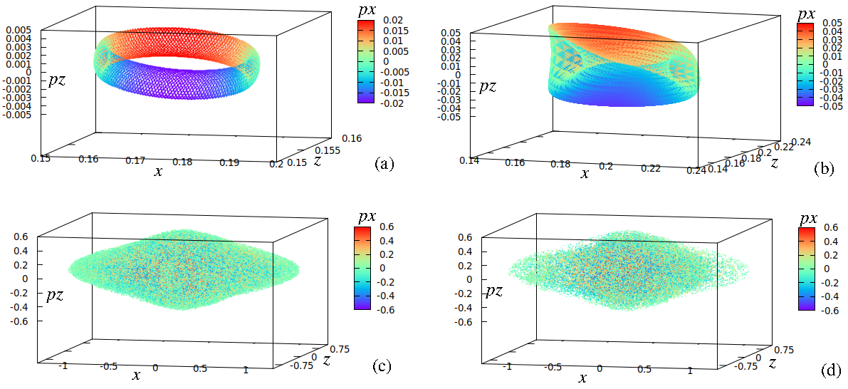
Figure 3: Ferrers bar: Poincaré sections of orbits close to x1v1 periodic orbits at E_J $=-0.3073$ (a), $-0.3023$ (b), $-0.2973$ (c) and $-0.2923$ (d). All of them have initial conditions of x1v1 perturbed in the $x$-direction by 0.1$x_{0}(\rm{x1v1})$. The x1v1 family at the corresponding energies is stable in (a) and (d) and complex unstable in (b) and (c).

It is obvious that, at least in this case, the regular or chaotic character in the vicinity of the periodic orbit, at the level of a perturbation of 10% of just one of the four initial conditions of it, is not associated with the value of the quantity $\Delta$. Even more, in some cases like the one presented in Fig. 2d and Fig. 3d, the orbit is not affected at all by the presence of the stable periodic orbit x1v1. Apart from the degree of complexity of the 3D projections of the regular structures around a stable (Fig. 3a) and a complex unstable (Fig. 3b) periodic orbit, the main difference in the structure of phase space between the two cases is found in the immediate neighbourhood of the periodic orbit, i.e. within a radius $r$ around it, as $r\rightarrow 0$. Around a stable periodic orbit we always find toroidal structures, while for tiny perturbations of the initial conditions of a complex unstable one, the consequents drift away from it without building a hole. In the case of the complex unstable periodic orbit at E_J =$-0.3023$, at which the regular structure of Fig. 3b also exists, a perturbation of $10^{-9}$ of its $x$ coordinate leads to an orbit with the Poincaré cross section we present in Fig. 4a. A spiral pattern around the initial conditions of the periodic orbit, like those encountered in previous studies (Papadaki et al., 1995; Katsanikas et al., 2011; Stöber and Bäcker, 2021), is discernible for the first 350 consequents (Fig. 4a). Then, gradually, a regular structure is formed with increasing integration time. Contrarily, around the complex unstable periodic orbit with E_J =$-0.2973$, in the case of the orbit in Fig. 3c, we do not observe a spiral pattern even for tiny perturbations. In Fig. 4b we give the first 200 consequents of such an orbit. We can only observe that the consequents depart from the periodic orbit along certain directions.

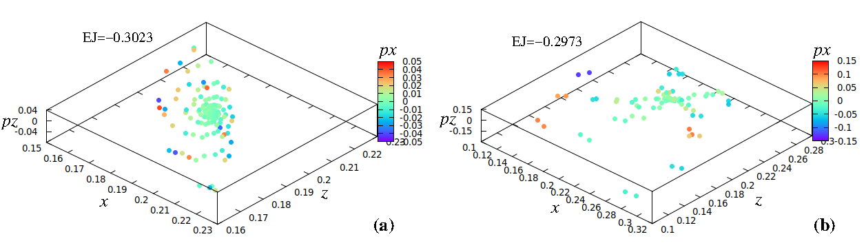
Figure 4: Ferrers bar: The first few hundreds of the consequents in the Poincaré sections of two orbits in the immediate neighbourhood of complex unstable x1v1 periodic orbits, to which we have applied just a tiny perturbation, of the order of $10^{-9}$ in the $x$ coordinate. In (a) E_J $=-0.3023$, as in Fig. 3b and in (b) E_J =$-0.2973$, as in Fig. 3c.

Beyond the $\Delta\!\!\rightarrow$S transition, in order to find regular orbits close to the now stable x1v1, i.e. quasi-periodic orbits trapped around it at E_J =$-0.2923$, we have to reduce the perturbation applied to the $x_{0}$ initial condition, to $0.02x_{0}\rm{(x1v1)}$. The toroidal structure we find in 4D has a hole, evident in the $(x,p_{x})$ projection. If we go back to the complex unstable region and we consider a complex unstable periodic orbit at E_J =$-0.2938$, where $\Delta$ is about the same as $\Delta$ at E_J $=-0.3023$ (Fig. 1), we do not find similar phase structures around the two complex unstable periodic orbits. In the smaller energy (E_J $=-0.3023$) we have encountered the orbit presented in Fig. 3b, with the GALI₂ shown in Fig. 2b by perturbing the $x$ coordinate by 10%. In the larger energy (E_J =$-0.2938$), by applying the same relative perturbation we find chaos. In this case, even if we reduce the perturbation in the $x$-direction to $0.001x_{0}\rm{(x1v1)}$, we find chaotic orbits. There is no symmetry in the phase space structure in the cases of the two periodic orbits with similar $\Delta$ (Eq. 4) values. This is better realized close to the transition points (S$\rightarrow\Delta$ and $\Delta\rightarrow$ S), where we observe that around the orbit with the larger E_J ​​ we find more chaos. We also find that beyond the $\Delta\rightarrow$S transition the volume of regular orbits around the stable periodic orbits is reduced. In most cases, this asymmetry reflects the different landscapes we encounter in the phase space region around the periodic orbits of a family at different E_J . Thus, by applying similar perturbations at different E_J we may enter a zone of influence of a stable periodic orbit or a chaotic sea. Nevertheless, within a time of interest for the specific physical problem, i.e. for 5 Gyr, orbits with initial conditions deviating from those of the complex unstable x1v1 by $0.05x_{0}\rm{(x1v1)}$ or $0.05z_{0}\rm{(x1v1)}$ are to a large degree bar-supporting.

The second $\Delta$ region in this model, is found for $-0.2673\lessapprox E_{J}\lessapprox-0.2328$, where we have again a S$\rightarrow\!\!\Delta\!\!\rightarrow$S transition. This time, the complex unstable region extends in a broader E_J range and the maximum $|\Delta|$ in it is much larger (Fig. 5).

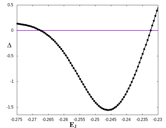
Figure 5: Ferrers bar: Variation of $\Delta$ (Eq. 4) for the x1v1 family of periodic orbits in the $-0.275\leq E_{J}\leq-0.23$ region. The heavy dots correspond to calculated periodic orbits. Those with $\Delta<0$ are complex unstable.

For orbits at these energies the dynamical time scales are large and to the same physical time correspond much less consequents. Perturbations of the stable orbits of the x1v1 family of the order of 0.1$x_{0}(\rm{x1v1})$ or 0.1$z_{0}(\rm{x1v1})$ in the $x$- or $z$-direction respectively, bring always the initial conditions in chaotic regions of phase space. In that sense, before the second S$\rightarrow\!\!\Delta$ transition of x1v1, at E_J $\approx-0.2673$, we enter chaotic seas by applying relatively smaller perturbations than to the initial conditions of the stable periodic orbits of the family before the first S$\rightarrow\!\!\Delta$ transition of x1v1, at E_J $\approx-0.3028$. By reducing the perturbations to 0.05$x_{0}(\rm{x1v1})$, or 0.05$z_{0}(\rm{x1v1})$, we find regular, i.e. quasi-periodic, orbits around stable x1v1 for E_J $<\!-0.2713$. Then, as we approach the critical E_J at $\approx-0.2673$, the perturbed by 5% orbits become chaotic, first along the $z$ direction, while even closer to it we have to reduce the perturbation even more in order to find close to the periodic orbits regular structures in phase space. In Fig. 6 we give the perturbed by 0.05$x_{0}(\rm{x1v1})$ (panels a to d) and 0.05$z_{0}(\rm{x1v1})$ (panels e to h) orbits, for E_J =$-0.27134$.

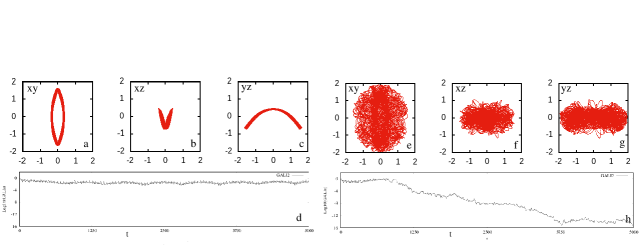
Figure 6: Ferrers bar: From (a) to (c) we give the $(x,y)$, $(x,z)$ and $(y,z)$ projections of an x1v1 orbit with E_J =$-0.27134$, perturbed by 0.05$x_{0}(\rm{x1v1})$ in the $x$ coordinate. They point to a quasi-periodic orbit trapped around the x1v1 periodic orbit, as its GALI₂ variation over a 5 Gyr period indicates in (d). (e) to (g): The corresponding projections for the x1v1 orbit perturbed by 0.05$z_{0}(\rm{x1v1})$ in the $z$ coordinate. The orbit behaves in a chaotic way, after an initial sticky phase, as its GALI₂ variation in (h) indicates.

The perturbed in the $x$-direction orbit has a typical quasi-periodic morphology as its $(x,y)$, $(x,z)$ and $(y,z)$ projections, in Fig. 6a, b and c respectively, show. The regular nature of the orbit is in agreement with the variation of its GALI₂ index in Fig. 6d. Contrarily, the orbit perturbed in the $z$-direction (Fig. 6e,f,g) is chaotic. The GALI₂ index (Fig. 6h) shows that after an initial sticky phase, the orbit has a chaotic behaviour. In order to find regular orbits when we perturb x1v1 in $z$ at this and larger E_J ​​, before the S$\rightarrow\!\!\Delta$ transition, we have to impose perturbations of the order of $10^{-3}z_{0}(\rm{x1v1})$ or smaller.

As we approach the critical E_J ​​, where we have the S$\rightarrow\!\!\Delta$ transition, the volume of phase space with regular orbits around a stable x1v1, shrinks. In parallel, there is an evolution of the morphology of tori structures, e.g. like the one given in Fig. 3a, towards a disky configuration. Nevertheless, we find a hole in the center of these structures. For example, if we perturb the initial conditions of a stable x1v1 orbit very close to the $\Delta$ region, at E_J =$-0.26753617$, by $0.001x_{0}\rm{(x1v1)}$, we find the orbit depicted in Fig. 7. We give the $(x,p_{x})$ and $(x,z)$ projections, in Fig. 7a and Fig. 7b respectively, with the consequents coloured according to their $p_{z}$ values.

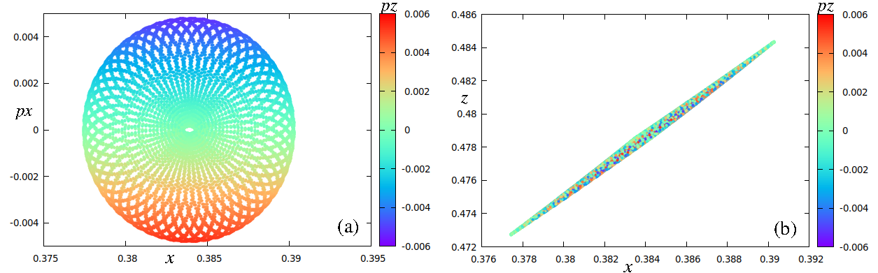
Figure 7: Ferrers bar: The $(x,p_{x})$ (a) and $(x,z)$ (b) projections of the orbit with initial conditions those of the stable x1v1 at E_J =$-0.26753617$, perturbed by $0.001x_{0}\rm{(x1v1)}$, form a very thin toroidal - disky, morphology. The consequents are coloured according to their $p_{z}$ values. The energy of the orbit is very close to the S$\rightarrow\!\!\Delta$ transition. For long integration times, all holes but the central in (a) are eventually filled.

Beyond the transition, in the immediate neighbourhood of the x1v1 orbits, which are now complex unstable, we encounter the known arrangement of the consequents in a spiral lay out (Papadaki et al., 1995; Katsanikas et al., 2011; Stöber and Bäcker, 2021), as in the case for E_J =$-0.26743617$, which we present in Fig. 8.

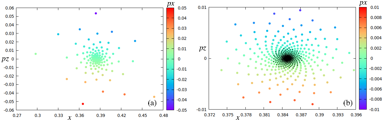
Figure 8: Ferrers bar: Perturbed x1v1 orbits at E_J =$-0.26743617$, just after the S$\rightarrow\!\!\Delta$ transition. (a) An orbit perturbed by $0.001x_{0}\rm{(x1v1)}$. (b) An orbit perturbed by $10^{-8}x_{0}\rm{(x1v1)}$. In (a) there are 120 consequents plotted, while in (b) 1800, the first 1600 of which are marked with black dots. For larger integration times both orbits become chaotic.

In Fig. 8a the x1v1 orbit is perturbed by $0.001x_{0}(\rm{x1v1})$. We observe the first 120 consequents, which are organized in a multi-spiral pattern with smooth colour variation along its arms. In this case, we give the $(x,p_{z})$ projection, in which the points are coloured according to the value of their $p_{x}$ coordinate. If we continue integrating the orbit, the consequents will build a cloud of points with mixed colours, namely the orbit will behave in a chaotic way. If we consider a tiny perturbation $10^{-8}x_{0}(\rm{x1v1})$, we find the corresponding representation of the Poincaré surface of section, which is given in Fig. 8b. The organization of the consequents in the depicted multi-spiral pattern lasts for about 1800 intersections, the 1600 of which are marked with black dots. This orbit, for larger integration times behaves also as a chaotic one.

We underline that in both cases the “regular” period of the orbits is much longer than the 5 Gyr time interval we are interested in, for finding bar-supporting orbits. However, as regards the properties of the dynamical system we study, we remark that the transition to chaos is more abrupt in the second than in the first case of the S$\rightarrow\!\!\Delta$ transitions we discussed. In neither case presented in Fig. 8 the long time integration results to the formation of invariant structures around the complex unstable periodic orbit, such as those encountered in Pfenniger (1985a) or Katsanikas et al. (2011). Having orbits, which behave initially as regular and later as chaotic, we can characterize them as sticky (Contopoulos and Harsoula, 2010). For E_J ​​’s away from the critical one, at which we have the second S$\rightarrow\!\!\Delta$ transition, we can hardly trace a spiral pattern in the surfaces of section of orbits close to x1v1, even if we apply very small perturbations.

The determination of the volume of phase space around a complex unstable periodic orbit, where we can find structure-supporting orbits, is a heavy task. Given that even small perturbations may well bring the initial conditions of the perturbed orbit to zones of influence of other orbital families, not necessarily simple periodic, it is not always clear to which degree the presence of a complex unstable periodic orbit is associated with the level of chaoticity of a nearby orbit. This is also indicated by the variation of its GALI₂ index.

For instance, in Fig. 9 we consider orbits in the neighbourhood of seven complex unstable periodic orbits in the E_J interval $-0.275\lessapprox E_{J}\lessapprox-0.23$ (Fig. 5) with initial conditions close to those of x1v1, but with $x_{0}=1.05x_{0}(\rm x1v1)$ or with $z_{0}=1.05z_{0}(\rm x1v1)$, and we plot the variation of their GALI₂ indicators within a 5 Gyr period. The panels on the left hand side correspond to the orbits perturbed by $\Delta x$, while on the right hand side to the orbits perturbed by $\Delta z$. The Jacobi constants and the $\Delta$ value of the corresponding complex unstable x1v1 periodic orbit are: In (a) and (b) E_J =$-0.26534465$ and $\Delta\approx-0.083$, in (c) and (d) $-0.25484465$ and $-0.951$ respectively, in (e) and (f) $-0.25334465$ and $-1.108$, in (g) and (h) $-0.24584465$ and $-1.557$, close to the largest $|\Delta|$, in (i) and (j) $-0.23984465$ and $-1.196$, in (k) and (l) $-0.23684465$ and $-0.786$, and finally in (m) and (n) $-0.23384465$ and $-0.276$.

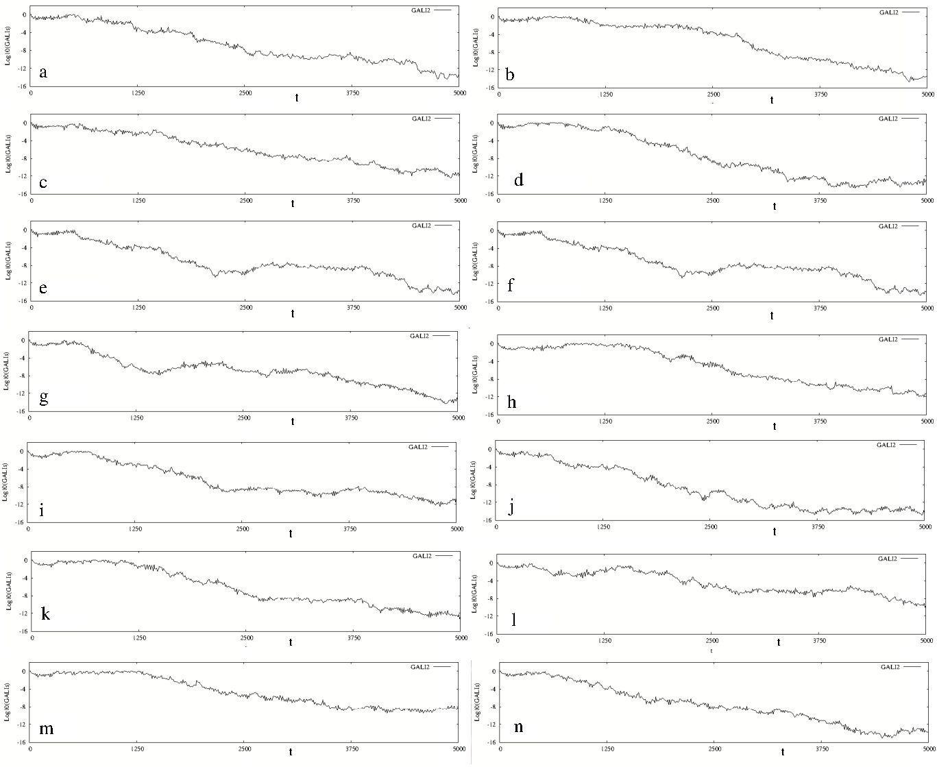
Figure 9: Ferrers bar: GALI₂ variation of orbits in the neighbourhood of complex unstable x1v1 orbits, perturbed by $0.05x_{0}\rm{(x1v1)}$ (left column) and by $0.05z_{0}\rm{(x1v1)}$ (right column). The variation of $\Delta$ of the corresponding periodic orbits can be deduced from Fig. 5 (the E_J ’s are given in the text). The panels closest to the maximum $|\Delta|$ are in the fourth row, i.e. in panels (g) and (h). In general the GALI₂ variation can be affected by the presence of other nearby families existing in phase space close to the periodic orbit.

In the left column of Fig. 9, we observe that there is always an almost horizontal part of the curves with the GALI₂ variation, which appears at the left side of each panel. This part corresponds to times of the order of 1 Gyr or less. For the dynamical time scales of these orbits, at the E_J we consider them, within this period we have only a few consequents, less than 20, which depart from the periodic orbit forming in general a spiral pattern, before they start behaving in a chaotic way. In panel (g), where we have a perturbed x1v1 orbit in the $x$-direction, we are closest to the maximum $|\Delta|$ of the region we study. We observe that the horizontal branch of its GALI₂ variation is, together with the one in panel (e), one of the shortest. However, for larger times in Fig. 9g, there is a second plateau, before the curve starts decreasing monotonically. Such variations make it even more difficult to link the values of $\Delta$ (Eq. 4) with the degree of chaoticity to the phase space around a complex unstable periodic orbit.

A characteristic example of a complicated landscape of the phase space in the neighbourhood of a complex unstable periodic orbit is given in Fig. 10. We present the $(x,z,p_{x},p_{z})$ Poincaré section of an orbit very close to the $\Delta\!\!\rightarrow$S transition, at the right hand side of the $\Delta$ region in Fig. 5, at E_J ​​= $-0.23283617$, where x1v1 has $\Delta=-0.092$.

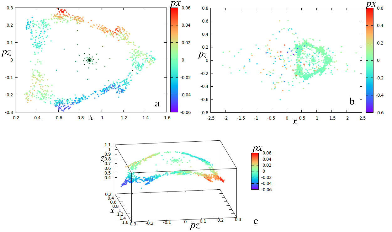
Figure 10: Ferrers bar: An orbit close to the x1v1 complex unstable periodic orbit, at E_J ​​= $-0.23283617$, near the $\Delta\!\!\rightarrow$S transition. The initial conditions of the orbit differ from those of the periodic one by $10^{-8}x_{0}$ in the $x$ coordinate. In (a) and (b) we give the $(x,p_{z})$ projection, with the consequents coloured according to their $p_{x}$ values, while in (c) the $(x,p_{z},z)$ projection, coloured again according to the $p_{x}$ values. In (a) and (c) we consider 1200 intersections with the $y$=0 plane, while in (b) 1600. The orbit drifts to a chaotic sea after forming first a spiral pattern and then remaining sticky in a zone around the periodic orbit.

We consider the periodic orbit and apply a tiny perturbation in its initial $x_{0}$ condition, namely $10^{-8}x_{0}(\rm{x1v1})$. The first 226 consequents of the orbit form a usual spiral pattern (central region of Fig. 10a), as they deviate away from the complex unstable x1v1. However, the breaking of the spiral pattern is not followed by a diffusion in a chaotic domain, but by the sticking of the orbit in a weakly chaotic zone surrounding a chain of stability islands. In Fig. 10a, we give the first 1200 consequents in the $(x,p_{z})$ projection, coloured according to their $p_{x}$ values. The first 226, building a 3-armed spiral pattern, are emphasized with black points. In Fig. 10b we give the first 1600 consequents and we observe how they diffuse in a broader chaotic sea. In Fig. 10c we present again the first 1200 consequents, but using the 3D $(x,p_{z},z)$ projection, also coloured according to their $p_{x}$ values. We realize that the consequents are practically on a warped-disky surface, reminiscent of the shape of the disky confined tori (Katsanikas et al., 2011).

We reach similar conclusions by studying perturbations in the $z$-direction. In Fig. 9, the right hand column with the GALI₂ indices refers to orbits with initial conditions close to the periodic orbits, perturbed in the $z$ direction by $0.05z_{0}\rm{(x1v1)}$. This time, from top to bottom, the horizontal part of the GALI₂ curves initially is reduced with increasing $|\Delta|$. However, in panel (h), close to the x1v1 orbit with the maximum $|\Delta|$, the perturbed by 5% in the $z$-direction orbit shows a more extended horizontal part, as does the orbit in panel (l). Such variations are again due to the presence of the orbits of other families in the neighbourhood of the periodic orbit we study.

Restoration of stability, for E_J $>-0.2328$, has also a gradual character. Just beyond the $\Delta\!\!\rightarrow$S transition, the “range of influence” of the stable periodic orbit is small. For E_J ​​=$-0.23234$, the tolerance of the perturbation of the $x_{0}$ initial condition, so that we find quasiperiodic orbits on tori with a smooth colour variation on them, is just $\Delta x\approx 0.0015x_{0}(\rm{x1v1})$. This orbit can be seen in Fig. 11a. For larger perturbations of $x_{0}$ the orbits are chaotic, with an initial sticky phase appearing up to a perturbation of $\Delta x\approx 0.05x_{0}(\rm{x1v1})$. In Fig. 11b, we give the first 600 consequents of the orbit, for which the perturbation of x1v1 is $0.002x_{0}(\rm{x1v1})$. During this period, the structure of phase space around the stable periodic orbit resembles the spiralling observed around a complex unstable one. For larger integration time a chaotic cloud is formed, similar to those depicted in Fig. 3c,d. Away from the transition to stability region, the phase space structure around the stable x1v1 orbits is characterized by stability islands of considerable sizes. For example, for E_J =$-0.22934$, if we perturb again the periodic orbit in $x$, we find tori of quasi-periodic orbits for perturbations up to about $0.5x_{0}(\rm{x1v1})$.

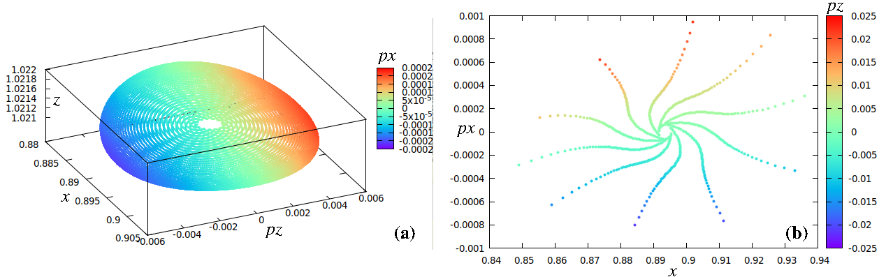
Figure 11: Ferrers bar: (a) The tiny torus of the quasiperiodic orbit with initial conditions of x1v1, perturbed by $0.0015x_{0}(\rm{x1v1})$, for E_J ​​=$-0.23234$. We use the $(x,p_{z},z)$ spatial projection and $p_{x}$ for giving colour to the consequents. (b) The first 600 consequents of another orbit, this time with a perturbation $0.002x_{0}(\rm{x1v1})$, at the same E_J ​​, in the $(x,p_{x})$ projection, coloured according to their $p_{z}$ value. They form a structure reminiscent of the spirals close to complex unstable periodic orbits. For longer integration times this orbit diffuses in the available phase space.

5.2 Complex Unstable regions in PERLAS spirals

In the PERLAS case the perturbative term is in the form of a spiral potential, in which the mass of the spiral ($M_{s}$), over the mass of the disc ($M_{d}$) is $M_{s}/M_{d}=0.04$ (model M4 in Chaves-Velasquez et al., 2019). The family of x1v1 periodic orbits is introduced in the same way as in the rotating Ferrers bar, namely as a bifurcation of the central family x1, at the vertical 2:1 resonance. The projections of the orbits of this family on the equatorial plane are elliptical-like. However, in the PERLAS potential, they are not aligned along an axis as in the case of a bar. Their orientation changes in such a way, as to support a bisymmetric set of logarithmic spiral arms (Chaves-Velasquez et al., 2019).

In the specific PERLAS model we study, the evolution of the stability of this family with E_J is also qualitative similar with that of the Ferrers bar we studied in the previous subsection (5.1). Namely, we find two S$\rightarrow\!\!\Delta\!\!\rightarrow$S transitions, for $-1354.3\lessapprox$ E_J $\lessapprox-1345.8$ and $-1208.7\lessapprox$ E_J $\lessapprox-1131.6$, in the units we use for this model (see figure 6 in Chaves-Velasquez et al., 2019). Taking into account that the center of the system is at E_J $\approx-1580$ and the Lagrangian point L4 at corotation, at E_J $\approx-1038$, the first complex unstable region is tiny in the energy range in which the families of the x1-tree extend. The quantity $\Delta$ (Eq. 4) in $-1354.3\lessapprox$ E_J $\lessapprox-1345.8$ has a variation similar to those in the complex unstable regions we presented in Fig. 1 and Fig. 5 for the Ferrers bar model, with a maximum $|\Delta|\approx 0.029$. In a 5 Gyr period, all orbits with initial conditions those of the complex unstable periodic orbits perturbed in the $x$-direction by $0.1x_{0}(\rm{x1v1})$ or in the $z$-direction by $0.1z_{0}(\rm{x1v1})$ behave apparently as regular and support the imposed 2-armed spiral pattern. We calculated their GALI₂ indices and we found variations indicating a regular behaviour.

The second complex unstable region ($-1208.7\lessapprox$ E_J $\lessapprox-1131.6$) is quite broad and the variation of $\Delta$ (Eq. 4), which is again U-shaped as in all previous cases, has a minimum $\Delta=-4.9$ at E_J $\approx-1165$. Let us first describe the evolution of structures in phase space close to the S$\rightarrow\!\!\Delta$ transition point at E_J = $-1208.7$. We study it by applying radial perturbations to the $x$ coordinate of the initial conditions of the x1v1 periodic orbit. For the sake of brevity in the case of the spiral PERLAS potential we will use for the presentation of our results mainly radial perturbations. We do so, because the problem of the orbital support of a galactic grand-design spiral pattern should be considered in a first approximation as a problem of finding perturbed orbits practically on the equatorial plane of the model.

Close to the transition point, at E_J $=-1210.228$, x1v1 is still stable. However, we find again that the extent of the region within which we find quasiperiodic orbits around x1v1, has been considerably reduced. Already a perturbation by $0.03x_{0}(\rm{x1v1})$ corresponds to a chaotic orbit, which visits all available phase space if integrated for long time, as we can see in Fig. 12a. The location of x1v1 in Fig. 12a is indicated with a heavy black dot at the left part of the figure. It is located at negative $x$, due to the way we define the Poincaré section in a clockwise rotating system. For a perturbation $0.01x_{0}(\rm{x1v1})$ we find a regular orbit, which is confined in a thin, warped, disky structure, which is not filled even after $10^{4}$ intersections (Fig. 12b). Only for perturbations of the order of $0.001x_{0}(\rm{x1v1})$, we encounter the known, characteristic structure of a torus in 3D projections with smooth colour variation in the fourth coordinate (Fig. 12c).

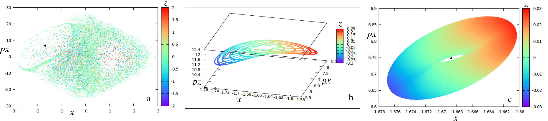
Figure 12: PERLAS potential: The cross sections of three orbits in the neighbourhood of the stable x1v1 periodic orbit at E_J = $-1210.228$, just before the S$\rightarrow\!\!\Delta$ transition. All of them are perturbations of the periodic orbit in the $x$ coordinate. In (a) by $x=0.03x_{0}(\rm{x1v1})$, in (b) by $0.01x_{0}(\rm{x1v1})$ and in (c) by $0.001x_{0}(\rm{x1v1})$. The area occupied by regular orbits around x1v1 is small. Black dots in (a) and (c) point to the location of the periodic orbit.

At a slightly larger E_J ​​, for E_J = $-1208.228$, the periodic orbit has become complex unstable, still being close to the S$\rightarrow\!\!\Delta$ transition. We find that only tiny perturbations of the $x_{0}$ initial condition of the periodic orbit result to the formation of spiral patterns around the periodic orbit in phase space (Papadaki et al., 1995; Katsanikas et al., 2011; Stöber and Bäcker, 2021). Nevertheless, even in these cases, the consequents eventually diffuse in phase space. A characteristic example is given in Fig. 13, where we present the cross section of the orbit with initial conditions those of the periodic orbit x1v1 perturbed by $0.001x_{0}(\rm{x1v1})$.

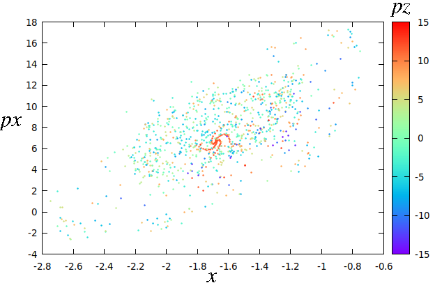
Figure 13: PERLAS potential: The $(x,p_{x})$ projection of the cross section of an orbit in the neighbourhood of the complex unstable x1v1 with E_J = $-1208.228$. The consequents are coloured according to their $p_{z}$ values. The orbit has the initial conditions of x1v1 perturbed by $0.001x_{0}(\rm{x1v1})$. A spiral pattern formed by the first 67 consequents is discernible in the middle of the figure.

As E_J increases, the phase space close to the complex unstable x1v1 periodic orbits becomes practically chaotic. The number of consequents arranged in a spiral pattern when we integrate orbits close to the periodic one, decreases. We can say that most complex unstable periodic orbits in the range $-1208.7<$ E_J < $-1131.6$ are found embedded in chaotic seas. The situation changes again as we approach the $\Delta\!\!\rightarrow$S transition, for E_J $\approx-1131.6$. For example, by considering perturbations $0.001x_{0}$ to the initial conditions of x1v1, we find invariant structures around the complex unstable periodic orbits for E_J $\gtrapprox-1134$. Their appearance is preceded by the presence of consequences confined for a few hundreds of intersections in an almost disky structure, before they eventually diffuse in phase space. Very close to the transition point, at E_J $=-1132.228$, we find in the neighbourhood of the periodic orbit the known wavy, disky structure in the 3D projection of the space of section, with a smooth colour variation across it, representing the fourth dimension (Katsanikas et al., 2011). A difference with previous cases is that the underlying spiral pattern followed by the consequents as they fill the area of the disky structure is one-armed. This is described in Fig. 14 for the x1v1 orbit perturbed by $0.001x_{0}(\rm{x1v1})$. The cross section is given in the $(x,p_{x})$ projection, while the colour of the points corresponds to their $p_{z}$ values. The consequents follow first an one-armed spiral from the center to the outer boundary of the disky structure and then continue spiralling inwards. This cycle is repeated until the surface of the disky structure is covered with points. We show this by plotting the first 25 consequents of the orbit in Fig. 14a with heavy black dots and connecting them with straight lines, and then in Fig. 14b, by plotting with red dots and lines the consequents from the 40th to the 61st one. We indicate with numbers some consequents in both panels, in order to facilitate understanding that the points follow spiral patterns. The black consequents follow a spiral outwards, while the red ones a spiral inwards. Following these first 61 successive intersections of the orbit with the space of section, one can appreciate the pattern followed by the consequents in forming the underlying disky structure.

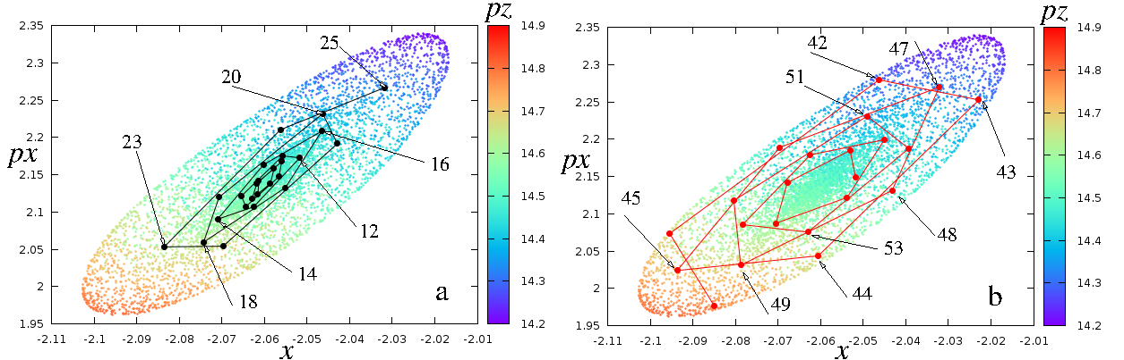
Figure 14: PERLAS potential: The disky structure with the smooth colour variation along its surface, formed by the consequents of the perturbed by $\Delta x=0.001x_{0}$ x1v1 orbit, at E_J = $=-1132.228$. We give the $(x,p_{x})$ projection and we colour the points according to their $p_{z}$ values (colour bar at the right hand side of the panels). The first 25 consequents are plotted in (a) with black dots and are connected with black lines and the consequents from the 40th to the 61st one are plotted with red dots and lines in (b). The disky structure is formed by the cosequents following successive cycles of spiralling outwards as in (a) and then spiralling inwards as in (b). We indicate with numbers, and arrows pointing to them, several consequents in both panels in order to understand the out- and inwards spiralling of the points.

Also in this model, the phase space structure in the neighbourhood of the orbits with the same $\Delta$ values in the descending and ascending parts of the ($\Delta$, E_J ​​) curve is not the same. We can draw only the general conclusion that regular structures are found only close to the stability transition points.

The evolution of the phase space beyond the $\Delta\!\!\rightarrow$S transition has also a gradual character. Just beyond the critical value (E_J $\approx-1131.6$), at E_J = $-1131.228$, orbits with $\Delta x\geqq 0.1x_{0}$ perturbations of the initial conditions of x1v1 are chaotic. Only for smaller perturbations of the $x$ initial condition we find quasi-periodic orbits. The extent of the zone occupied by regular orbits around stable x1v1 orbits increases, as in the cases we studied in the Ferrers bar potential, for larger E_J ​​’s.

5.2.1 Practical implications

Besides the knowledge of the long-term evolution of the phase space structure in the neighbourhood of complex unstable periodic orbits, of special importance for Galactic Dynamics is the behaviour of the orbits during the time within which a spiral pattern is expected to survive. An upper limit for this can be considered a 5 Gyr period (Sellwood, 2011; Dobbs and Baba, 2014). During this time interval, all orbits in the first complex unstable region of x1v1, for $-1354.3\lessapprox$ E_J $\lessapprox-1345.8$, with initial conditions those of the periodic orbit perturbed by $0.1x_{0}(\rm{x1v1})$, can hardly be distinguished from quasi-periodic orbits. During the same time interval, the perturbed in the same way x1v1 orbits in the second complex unstable region, $-1208.7\lessapprox$ E_J $\lessapprox-1131.6$, evolve as shown in Fig. 15. There we present 6 orbits, the E_J of which and the $\Delta$ values of the corresponding orbits successively are: E_J = $-1209.228\;(\Delta=0.155)\;\rm{(a)},-1208.228\;(\Delta=-0.006)\;\rm{(b)},-1191.228\;(\Delta=-2.821)\;\rm{(c)},-1166.228\;(\Delta=-4.858)\;\rm{(d)},-1132.228\;(\Delta=0.131)$ (e) and $-1131.228\;(\Delta=0.157)$ (f). For each one of them we give the three projections, $(x,y),(x,z)$ and $(y,z)$ and below them the evolution of their GALI₂ index during a 5 Gyr period.

Figure 15: PERLAS potential: Perturbed by 10% in the x coordinate x1v1 orbits. For each one of them we present the three projections $(x,y)$, $(x,z)$, $(y,z)$ and the evolution of GALI₂ during a 5 Gyr period. They are at E_J $-1209.228$ (a), $-1208.228$ (b), $-1191.228$ (c), $-1166.228$ (d), $-1132.228$ (e) and $-1131.228$ (f). The corresponding periodic orbits in (a) and (f) are stable, while in all other cases complex unstable. All depicted orbits reinforce at some degree the spiral pattern.

The periodic orbits existing at the E_J ​’s of the non-periodic orbits depicted in Fig. 15a and Fig. 15f are stable, while all other cases (Fig. 15b,c,d,e) are complex unstable. Both the morphology and the variation of the GALI₂ indicators of the two orbits in the neighbourhood of the stable periodic orbits indicate a sticky behaviour. We also observe that the orbits close to the complex unstable periodic ones never become strongly chaotic. However, although the perturbation of one of the initial conditions of the periodic orbit by 10% leads to realistic initial conditions of an orbit potentially supporting the spiral structure, it is not necessarily associated with the immediate environment of the complex unstable periodic orbit. Such a perturbed orbit may belong to an invariant torus around another, stable, periodic orbit existing in the region, or it may become an orbit trapped in a nearby sticky zone. This means that we encounter a situation similar to the perturbed periodic orbits of the Ferrers bar.

For example, the consequents of the orbit in Fig. 15b, in its $(x,p_{x})$ projection of the Poincaré surface of section during the 5 Gyr period, are stuck in the region delimited by the heavy black dots in Fig. 16. These latter, are the consequents of the orbit during the time interval 3.3 to 4.5 Gyr, which appear stuck along this ring. As the variation of the GALI₂ of the orbit in Fig. 15b indicates, the orbit is weakly chaotic, but it does not diffuse in phase space. This secures for this period the confinement of the orbit in the $(x,y)$ projection on the equatorial plane in an annular region, which retains the orientation of the x1v1 periodic orbit with the same E_J ​​. This is a useful result, since x1v1 participates in the reinforcement of a bisymmetric, three dimensional, spiral pattern by means of the mechanism of “precessing ellipses” (Kalnajs, 1973), as shown by Chaves-Velasquez et al. (2019). The importance of orbits, which remain encapsulated in regions of phase space for significant time intervals has been underlined in studies by Muzzio (2017, 2018). Our analysis leads us to the conclusion that even in the complex unstable parts of a family there are non-periodic orbits which may contribute to the reinforcement of the spiral pattern for considerable time intervals. If we continue integrating the orbit for longer times we find that it diffuses visiting all available phase space (Fig. 16). However, this happens for non-realistic time scales, of the order of several Hubble times.

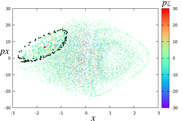
Figure 16: PERLAS potential: The $(x,p_{x})$ projection of the Poincaré surface of section of the orbit in Fig. 15b. The consequents are coloured according to their $p_{z}$ coordinate. During a 5 Gyr period the consequents are found confined within a ring-like structure delimited by the consequents of the orbit during the time interval 3.3 to 4.5 Gyr. This trapping of the consequents in a specific region of phase space allows the orbit to be spiral-supporting during this period.

6 Conclusions

We have investigated the phase space in the neighbourhood of complex unstable periodic orbits in two galactic type models, that support structures similar to those observed in disc galaxies. The models rotate with a constant pattern speed. The first one refers to the 3D dynamics of a bar, represented by a Ferrers bar, while the second to a 3D spiral PERLAS potential with two arms. In both cases we have examined the phase space close to periodic orbits of x1v1, which is a family introduced in the system as bifurcation of the central family x1, at its vertical 2:1 resonance. Orbits of this family are associated with the presence of a peanut, or X-shaped, bulge in the side-on view of the Ferrers model (Patsis et al., 2002; Patsis and Katsanikas, 2014) and with the enhancement of the spiral arms in the PERLAS potential (Chaves-Velasquez et al., 2019). Our main conclusions are the following:

1. The structure of the phase space in the neighbourhood of successive orbits of the x1v1 family in both models presents similar features, as the stability of the family experiences a S$\rightarrow\!\!\Delta\!\!\rightarrow$S transition with increasing E_J ​​. The evolution of the phase space structure can be summarized as follows:

   • Before the S$\rightarrow\!\!\Delta$ transition, the volume of regular orbits around the stable representatives of x1v1 decreases with increasing E_J ​​. Approaching the critical point, we have to decrease the perturbations we apply to one of the four initial conditions in order to find in the Poincaré spaces of section toroidal surfaces with smooth colour variation on them. Simultaneously the tori (as e.g. in Fig. 3a) become flatter, tending to become disky.

   • Just beyond the S$\rightarrow\!\!\Delta$ transition, around the complex unstable periodic orbits we find regular structures, namely disky confined tori (Pfenniger, 1985a, b; Katsanikas et al., 2011). There is an internal structure on them, in the sense that the consequents cover the surfaces of the confined tori following specific spiral patterns. The number of the arms of these spiral patterns varies.

   • A next phase in the evolution of the phase space structure in the neighbourhood of the x1v1 periodic orbits, appears as we depart from the S$\rightarrow\!\!\Delta$ transition point towards larger energies, keeping the relative perturbation constant. We find then consequents initially building spiral patterns with smooth colour variation along their arms, which later diffuse in phase space building clouds of scattered points, filling the available volume of the phase space, limitted by the surface of zero velocity.

   • For the largest part of a $\Delta$ region, integrating orbits in the immediate neighbourhood of the x1v1 periodic orbits leads to clouds of scattered points in the Poincaré cross sections. However, in many cases the orbits remain confined during a significant period within a certain subset of the 4-dimensional space. This plays a major role for practical applications.

   • Close to the $\Delta\!\!\rightarrow$S transition the phase space is organized again, however within small volumes around the complex unstable periodic orbit. Namely, we encounter again disky confined tori.

   • Finally, beyond the $\Delta\!\!\rightarrow$S transition, in the region where the family is again stable, the restoration of order has again a gradual character. The radius within which we find regular orbits around the periodic orbit increases with E_J ​​.

2. The shrinking of the volume occupied by regular orbits around the stable x1v1 periodic orbits and the evolution of the tori towards a disky morphology as we approach the critical energy for a S$\rightarrow\!\!\Delta$ transition, has been encountered in all studied cases. This is the second case we know that the deformation of a phase space structure close to a periodic orbit as the energy varies, foretells an impending change of stability (the first case has been presented by Patsis and Katsanikas, 2014, for changes in the topology of invariant tori before a S$\rightarrow$U transition).

3. Within an E_J interval in which the x1v1 family is complex unstable, orbits in the neighbourhood of periodic orbits with the same $\Delta$ (Eq. 4), subject to the same amount of relative perturbations, do not have the same degree of chaoticity. In the cases we studied, they appear more chaotic in the ascending part of the U-type curve of the (E_J ​​,$\Delta$) diagrams, towards the critical point of the $\Delta\rightarrow$S transition. In that respect, there is no perfect symmetry in the phase space structures around complex unstable periodic orbits with the same $\Delta$.

4. We underline the role of the phase space environment around a periodic orbit for the determination of the behaviour of the perturbed orbits. In many cases displacements of the initial conditions of a periodic orbit along a certain direction, may bring the initial conditions of the perturbed orbit in zones of influence of other periodic orbits (stable or unstable). The variation of the GALI₂ indices may warn us about such cases.

5. In both models, many orbits eventually expressing a chaotic character are structure-supporting within a 5 Gyr period. Especially for the spiral PERLAS potential, we conclude that even in the larger complex unstable energy interval, there are orbits relatively close to complex unstable periodic orbits, which contribute to the reinforcement of the spiral arms of the model for considerable time intervals.

6. Supporting further the above conclusion, we note that the orbits close to the periodic orbits of the small complex unstable energy intervals in both models, can hardly be distinguished from regular during a 5 Gyr period.

Acknowledgements

We thank G. Contopoulos and M. Katsanikas for fruitful discussions and useful comments. This work has been carried out in the frame of the project “Numerical investigation of the impact of Complex Instability to the phase space structure of Dynamical Systems” of the Research Center for Astronomy of the Academy of Athens. L.C.V thanks the Fondo Nacional de Financiamiento para la Ciencia, La Tecnología y la innovación "FRANCISCO JOSÉ DE CALDAS", MINCIENCIAS, and the VIIS for the economic support of this research. L.C.V acknowledges the support of the postdoctoral Fellowship of DGAPA-UNAM, Mexico. Ch.S. acknowledges support by the Research Committee (URC) of the University of Cape Town.

References

- Allen and Santillan (1991) Allen, C., Santillan, A., 1991. An improved model of the galactic mass distribution for orbit computations. RMxAA 22, 255.
- Benettin et al. (1980) Benettin, G., Galgani, L., Giorgilli, A., Strelcyn, J.M., 1980. Lyapunov characteristic exponents for smooth dynamical systems and for Hamiltonian systems - A method for computing all of them. I - Theory. II - Numerical application. Meccanica 15, 9–30.
- Broucke (1969) Broucke, R., 1969. Periodic orbits in the elliptic restricted three-body problem. NASA Tech. Rep. 32-1360, 1–125. doi:10.2514/3.5267.
- Chaves-Velasquez et al. (2019) Chaves-Velasquez, L., Patsis, P.A., Puerari, I., Moreno, E., Pichardo, B., 2019. Dynamics of Thick, Open Spirals in PERLAS Potentials. ApJ 871, 79. doi:10.3847/1538-4357/aaf6a6, arXiv:1812.04068.
- Contopoulos (1986) Contopoulos, G., 1986. Qualitative changes in 3-dimensional dynamical systems. Astron. Astrophys. 161, 244--256.
- Contopoulos (2002) Contopoulos, G., 2002. Order and chaos in dynamical astronomy, Springer.
- Contopoulos and Giorgilli (1988) Contopoulos, G., Giorgilli, A., 1988. Bifurcations and complex instability in a 4-dimensional symplectic mapping. Meccanica 23, 19--28. doi:10.1007/BF01561006.
- Contopoulos and Grosbol (1989) Contopoulos, G., Grosbol, P., 1989. Orbits in barred galaxies. Astron. Astrophys. Rev. 1, 261--289. doi:10.1007/BF00873080.
- Contopoulos and Harsoula (2010) Contopoulos, G., Harsoula, M., 2010. Stickiness effects in chaos. Celestial Mechanics and Dynamical Astronomy 107, 77--92. doi:10.1007/s10569-010-9282-6.
- Contopoulos and Magnenat (1985) Contopoulos, G., Magnenat, P., 1985. Simple Three-Dimensional Periodic Orbits in a Galactic-Type Potential. Celestial Mechanics 37, 387--414. doi:10.1007/BF01261627.
- Delis and Contopoulos (2016) Delis, N., Contopoulos, G., 2016. Analytical and numerical manifolds in a symplectic 4-D map. Celestial Mechanics and Dynamical Astronomy 126, 313--337. doi:10.1007/s10569-016-9697-9.
- Dobbs and Baba (2014) Dobbs, C., Baba, J., 2014. Dawes Review 4: Spiral Structures in Disc Galaxies. PASA 31, e035. doi:10.1017/pasa.2014.31, arXiv:1407.5062.
- Hadjidemetriou (1975) Hadjidemetriou, J.D., 1975. The Stability of Periodic Orbits in the Three-Body Problem. Celestial Mechanics 12, 255--276. doi:10.1007/BF01228563.
- Heggie (1985) Heggie, D.C., 1985. Bifurcation at Complex Instability. Celestial Mechanics 35, 357--382. doi:10.1007/BF01227832.
- Jorba and Ollé (2004) Jorba, À., Ollé, M., 2004. Invariant curves near Hamiltonian Hopf bifurcations of four-dimensional symplectic maps. Nonlinearity 17, 691--710. doi:10.1088/0951-7715/17/2/019.
- Kalnajs (1973) Kalnajs, A.J., 1973. Spiral Structure Viewed as a Density Wave. Proceedings of the Astronomical Society of Australia 2, 174--177. doi:10.1017/S1323358000013461.
- Katsanikas and Patsis (2011) Katsanikas, M., Patsis, P.A., 2011. The Structure of Invariant Tori in a 3d Galactic Potential. International Journal of Bifurcation and Chaos 21, 467. doi:10.1142/S0218127411028520, arXiv:1009.1993.
- Katsanikas et al. (2011) Katsanikas, M., Patsis, P.A., Contopoulos, G., 2011. The Structure and Evolution of Confined Tori Near a Hamiltonian Hopf Bifurcation. International Journal of Bifurcation and Chaos 21, 2321. doi:10.1142/S0218127411029811.
- Katsanikas et al. (2013) Katsanikas, M., Patsis, P.A., Contopoulos, G., 2013. Instabilities and Stickiness in a 3d Rotating Galactic Potential. International Journal of Bifurcation and Chaos 23, 1330005. doi:10.1142/S021812741330005X, arXiv:1201.2108.
- Magnenat (1982a) Magnenat, P., 1982a. Numerical Study of Periodic Orbit Properties in a Dynamical System with Three Degrees of Freedom. Celestial Mechanics 28, 319--343. doi:10.1007/BF01243741.
- Magnenat (1982b) Magnenat, P., 1982b. Periodic orbits in triaxial galactic models. Astron. Astrophys. 108, 89--94.
- Manos and Athanassoula (2011) Manos, T., Athanassoula, E., 2011. Regular and chaotic orbits in barred galaxies - I. Applying the SALI/GALI method to explore their distribution in several models. MNRAS 415, 629--642. doi:10.1111/j.1365-2966.2011.18734.x, arXiv:1102.1157.
- Martinet and de Zeeuw (1988) Martinet, L., de Zeeuw, T., 1988. Orbital stability in rotating triaxial stellar systems. Astron. Astrophys. 206, 269--278.
- Martinet and Pfenniger (1987) Martinet, L., Pfenniger, D., 1987. Complex instability around the rotation axis of stellar systems. I - Galactic potentials. Astron. Astrophys. 173, 81--85.
- Miyamoto and Nagai (1975) Miyamoto, M., Nagai, R., 1975. Three-dimensional models for the distribution of mass in galaxies. PASJ 27, 533--543.
- Muzzio (2017) Muzzio, J.C., 2017. Partially chaotic orbits in a perturbed cubic force model. MNRAS 471, 4099--4110. doi:10.1093/mnras/stx1922, arXiv:1707.08156.
- Muzzio (2018) Muzzio, J.C., 2018. Chaotic orbits obeying one isolating integral in a four-dimensional map. MNRAS 473, 4636--4643. doi:10.1093/mnras/stx2653, arXiv:1710.03360.
- Ollé and Pacha (1999) Ollé, M., Pacha, J.R., 1999. The 3D elliptic restricted three-body problem: periodic orbits which bifurcate from limiting restricted problems. Complex instability. Astron. Astrophys. 351, 1149--1164.
- Ollé et al. (2004) Ollé, M., Pacha, J.R., Villanueva, J., 2004. Motion close to the Hopf Bifurcation Of the vertical family of periodic orbits of L4. Celestial Mechanics and Dynamical Astronomy 90, 87--107. doi:10.1007/s10569-004-1592-0.
- Olle and Pfenniger (1995) Olle, M., Pfenniger, D., 1995. Bifurcation at Complex Instability, in: Simo, C. (Ed.), Hamiltonian Systems with Three or More Degrees of Freedom, pp. 518--522.
- Olle and Pfenniger (1998) Olle, M., Pfenniger, D., 1998. Vertical orbital structure around the Lagrangian points in barred galaxies. Link with the secular evolution of galaxies. Astron. Astrophys. 334, 829--839.
- Papadaki et al. (1995) Papadaki, H., Contopoulos, G., Polymilis, C., 1995. Complex instability, in: Roy, A., Steves, B. (Eds.), From Newton to Chaos, pp. 485--494.
- Patsis and Grosbol (1996) Patsis, P.A., Grosbol, P., 1996. Thick spirals: dynamics and orbital behavior. Astron. Astrophys. 315, 371--383.
- Patsis and Harsoula (2018) Patsis, P.A., Harsoula, M., 2018. Building CX peanut-shaped disk galaxy profiles. The relative importance of the 3D families of periodic orbits bifurcating at the vertical 2:1 resonance. Astron. Astrophys. 612, A114. doi:10.1051/0004-6361/201731114, arXiv:1804.06199.
- Patsis and Katsanikas (2014) Patsis, P.A., Katsanikas, M., 2014. The phase space of boxy-peanut and X-shaped bulges in galaxies - I. Properties of non-periodic orbits. MNRAS 445, 3525--3545. doi:10.1093/mnras/stu1988.
- Patsis et al. (2002) Patsis, P.A., Skokos, C., Athanassoula, E., 2002. Orbital dynamics of three-dimensional bars - III. Boxy/peanut edge-on profiles. MNRAS 337, 578--596. doi:10.1046/j.1365-8711.2002.05943.x.
- Patsis and Zachilas (1990) Patsis, P.A., Zachilas, L., 1990. Complex instability of simple periodic orbits in a realistic two-component galactic potential. Astron. Astrophys. 227, 37--48.
- Patsis and Zachilas (1994) Patsis, P.A., Zachilas, L., 1994. Using Color and Rotation for Visualizing Four-Dimensional Poincare Cross-Sections. International Journal of Bifurcation and Chaos 6, 1399--1424. doi:10.1142/S021812749400112X.
- Pérez-Villegas et al. (2012) Pérez-Villegas, A., Pichardo, B., Moreno, E., Peimbert, A., Velázquez, H.M., 2012. Pitch Angle Restrictions in Late-type Spiral Galaxies Based on Chaotic and Ordered Orbital Behavior. ApJL 745, L14. doi:10.1088/2041-8205/745/1/L14, arXiv:1112.3510.
- Pfenniger (1984) Pfenniger, D., 1984. The 3D dynamics of barred galaxies. Astron. Astrophys. 134, 373--386.
- Pfenniger (1985a) Pfenniger, D., 1985a. Numerical study of complex instability. I - Mappings. Astron. Astrophys. 150, 97--128.
- Pfenniger (1985b) Pfenniger, D., 1985b. Numerical study of complex instability. II. Barred galaxy bulges. Astron. Astrophys. 150, 112--128.
- Pfenniger (1987) Pfenniger, D., 1987. Complex instability around the rotation axis of stellar systems. II - Rotating oscillators. Astron. Astrophys. 180, 79--93.
- Pichardo et al. (2003) Pichardo, B., Martos, M., Moreno, E., Espresate, J., 2003. Nonlinear Effects in Models of the Galaxy. I. Midplane Stellar Orbits in the Presence of Three-dimensional Spiral Arms. ApJ 582, 230--245. doi:10.1086/344592, arXiv:astro-ph/0208136.
- Rubin et al. (1980) Rubin, V.C., Ford, W. K., J., Thonnard, N., 1980. Rotational properties of 21 SC galaxies with a large range of luminosities and radii, from NGC 4605 (R=4kpc) to UGC 2885 (R=122kpc). ApJ 238, 471--487. doi:10.1086/158003.
- Schmidt (1956) Schmidt, M., 1956. A model of the distribution of mass in the Galactic System. BAIN 13, 15.
- Sellwood (2011) Sellwood, J.A., 2011. The lifetimes of spiral patterns in disc galaxies. MNRAS 410, 1637--1646. doi:10.1111/j.1365-2966.2010.17545.x, arXiv:1008.2737.
- Skokos (2001) Skokos, C., 2001. On the stability of periodic orbits of high dimensional autonomous Hamiltonian systems. Physica D Nonlinear Phenomena 159, 155--179. doi:10.1016/S0167-2789(01)00347-5.
- Skokos (2010) Skokos, C., 2010. The Lyapunov Characteristic Exponents and Their Computation. Lecture Notes in Physics Berlin Springer Verlag 790, 63--135. doi:10.1007/978-3-642-04458-8_2.
- Skokos et al. (2007) Skokos, C., Bountis, T.C., Antonopoulos, C., 2007. Geometrical properties of local dynamics in Hamiltonian systems: The Generalized Alignment Index (GALI) method. Physica D Nonlinear Phenomena 231, 30--54. doi:10.1016/j.physd.2007.04.004, arXiv:0704.3155.
- Skokos and Manos (2016) Skokos, C., Manos, T., 2016. The Smaller (SALI) and the Generalized (GALI) Alignment Indices: Efficient Methods of Chaos Detection. Lect. Not. Phys. 915, 129--181.
- Skokos et al. (2002) Skokos, C., Patsis, P.A., Athanassoula, E., 2002. Orbital dynamics of three-dimensional bars - I. The backbone of three-dimensional bars. A fiducial case. MNRAS 333, 847--860. doi:10.1046/j.1365-8711.2002.05468.x, arXiv:astro-ph/0204077.
- Stöber and Bäcker (2021) Stöber, J., Bäcker, A., 2021. Geometry of complex instability and escape in four-dimensional symplectic maps. Phys. Rev. E 103, 042208. doi:10.1103/PhysRevE.103.042208, arXiv:2009.00970.
- van der Meer (1985) van der Meer, J.C., 1985. The Hamiltonian Hopf bifurcation, Springer,. volume 1160 of Lecture Notes in Mathematics.
- Zachilas et al. (2013) Zachilas, L., Katsanikas, M., Patsis, P.A., 2013. The Structure of Phase Space Close to Fixed Points in a 4d Symplectic Map. International Journal of Bifurcation and Chaos 23, 1330023. doi:10.1142/S0218127413300231, arXiv:1205.4575.
- Zachilas (1988) Zachilas, L.G., 1988. Numerical and Theoretical Study of 3D Stellar Systems (in Greek). PhD Thesis, University of Athens, Greece .
- Zachilas (1993) Zachilas, L.G., 1993. Complex instability. Astron. Astrophys. Sup. Ser. 97, 549--558.