Novel Bayesian neural network based approach for nuclear charge radii

Abstract

Charge radius is one of the most fundamental properties of a nucleus. However, a precise description of the evolution of charge radii along an isotopic chain is highly nontrivial, as reinforced by recent experimental measurements. In this paper, we propose a novel approach which combines a three-parameter formula and a Bayesian neural network. We find that the novel approach can describe the charge radii of all $A\geq 40$ and $Z\geq 20$ nuclei with a root-mean-square deviation about 0.015 fm. In particular, the charge radii of the calcium isotopic chain are reproduced very well, including the parabolic behavior and strong odd-even staggerings. We further test the approach for the potassium isotopes and show that it can describe well the experimental data within uncertainties.

I Introduction

Nuclear charge radius, as one of the most fundamental properties of a nucleus, plays a vital role in our understanding of the complex dynamics of atomic nuclei and in showcasing various nuclear structure phenomena, such as neutron halo  Nortershauser et al. (2009), shape coexistence and staggering Yang et al. (2016); Marsh et al. (2018), odd-even staggering de Groote et al. (2020), and nuclear magic numbers Kreim et al. (2014); Gorges et al. (2019). Lately, remarkable progress has been made in measuring the charge radii of those nuclei far from the $\beta$-stability line Angeli and Marinova (2013); Koszorús et al. (2021); Day Goodacre et al. (2021); Li et al. (2021). Although the global features of nuclear charge radii can be easily understood, e.g., $R\propto A^{1/3}$ or $Z^{1/3}$, with $Z$ and $A$ the proton and mass numbers, there exist some fine structures that have eluded a complete understanding, e.g., the parabolic-like behavior and strong odd-even staggerings between ⁴⁰Ca and ⁴⁸Ca, and the abrupt increase from ⁴⁸Ca to ⁵²Ca, with the latter being a candidate of doubly magic nuclei Huck et al. (1985); Wienholtz et al. (2013); Rosenbusch et al. (2015). The charge radii of potassium isotopes, which have been recently measured Koszorús et al. (2021); Kreim et al. (2014), show features below and above $N=28$ similar to those of calcium isotopes.

Many methods have been developed to predict nuclear charge radii, ranging from liquid drop models Weizsacker (1935); Brown et al. (1984), phenomenological parametrizations Nerlo-Pomorska and Pomorski (1994); Zhang et al. (2002); Wang and Li (2013); Sheng et al. (2015), sophisticated mean-field models Geng et al. (2005); Goriely et al. (2016); Peña Arteaga et al. (2016); Sarriguren (2019), to $ab$ $initio$ calculations with chiral effective field theory interactions Ekström et al. (2015). Most of these methods can describe the available data with a root-mean-square (RMS) deviation ranging from 0.07 to 0.02 fm. Nevertheless, none of them can provide satisfactory descriptions of the striking behavior of charge radii in calcium or potassium isotopes Garcia Ruiz et al. (2016); Koszorús et al. (2021). Recently, by adding a semi-microscopic correction originating from the Cooper pair condensation, a modified relativistic mean field plus BCS (RMF(BCS)*) ansatz has been proposed to describe the charge radii of the calcium An et al. (2020) and potassium An et al. (2021) isotopic chains.

In recent years, machine learning methods have found wide and successful applications in physics Carleo et al. (2019); Bourilkov (2020); Bedolla-Montiel et al. (2021); Bedaque et al. (2021). In particular, Bayesian neural networks (BNNs), because of their ability to combine the strengths of artificial neural networks (ANNs) as “universal approximators” Hornik et al. (1989) and stochastic modeling, have been successfully applied to study various nuclear properties, such as masses Utama et al. (2016a); Niu and Liang (2018), incomplete fission yields wang et al. (2019), charge yields of fission fragments Qiao et al. (2021), $\beta$-decay half-lives Niu et al. (2019), nucleon axial form factor Alvarez-Ruso et al. (2019), proton radius Graczyk and Juszczak (2014), charge radii Utama et al. (2016b), and nuclear liquid-gas phase transition Wang et al. (2020). In Ref. Utama et al. (2016b), the proton number $Z$ and mass number $A$ of a nucleus are used as inputs to train a BNN, achieving a relatively good description of charge radii and reducing the RMS deviation by about 50% in comparison with the underlying relativistic mean field (RMF) model. However, the BNN method fails to describe odd-even staggerings, in particular, those of calcium isotopes. Motivated by the success of Refs. An et al. (2020, 2021), we propose to improve the BNN method using the so-called feature engineering technique to create two new input features, $\delta$ and $P$, from $Z$ and $A$. We will show that the refined BNN method can not only achieve a much improved description of experimental charge radii Angeli and Marinova (2013); Day Goodacre et al. (2021); Li et al. (2021) but also can make reliable predictions for calcium and potassium isotopes with controlled uncertainties, which agree well with the latest experimental data Koszorús et al. (2021); Li et al. (2021).

This article is organized as follows. In Sec. II, we construct the refined Bayesian neural network and explain how we categorize experimental charge radii for training and validation. Results and discussions are presented in Sec. III, followed by a short summary in Sec. IV.

II Theoretical Formalism

Similarly to Ref. Utama et al. (2016b), our purpose is to combine a theoretical model of charge radii and a Bayesian neural network to improve the description of nuclear charge radii. In our approach, the BNN is used to simulate the residuals between the theoretical predictions and the corresponding experimental data. In the following, we explain how to choose the theoretical model and how to construct the BNN.

As mentioned in the Introduction, a large number of microscopic and macroscopic models have been developed to describe atomic nuclei and most of them can provide reasonably good description of nuclear charge radii Geng et al. (2005); Utama et al. (2016b); Li et al. (2021). While the macroscopic models are much more convenient for practical applications, the microscopic models such as the RMF model Geng et al. (2005) are rather time consuming but contain more physics such as shell effects or pairing effects. However, in the present work, we prefer to include these effects not in the underlying theoretical model but only via the inputs for the BNN to explore whether these effects can be learned by the BNN. Therefore,in this work, we choose the isospin-dependent NP formula developed by Nerlo-Pomorska and Pomorski Nerlo-Pomorska and Pomorski (1994):

$$R_{\mathrm{NP}}(Z,A)=r_{A}A^{\frac{1}{3}}\left[1-b(\frac{N-Z}{A})+\frac{c}{A}\right],$$ (1)

where $r_{A}$ = 0.966 fm, b = 0.182, and c = 1.652 Bayram et al. (2013). This formula can describe nuclear charge radii at a level similar to the more sophisticated relativistic mean field model Utama et al. (2016b).

There are two main components in the BNN Neal (1996): one is the artificial neural network and the other is the Bayesian inference system. As shown in Fig. 1, the artificial neural network we use is a fully connected feed-forward artificial neural network with one hidden layer. Mathematically, it has the following form:

$$f(x,\omega)=a+\sum\limits_{j=1}\limits^{H}b_{j}\tanh(c_{j}+\sum\limits_{i=1}\limits^{I}d_{ji}x_{i}),$$ (2)

where the parameters of the neural network are $\omega=({a,b_{j},c_{j},d_{ji}}$), $I$ is the number of input layer neurons, $H$ is the number of hidden layer neurons, and $x$ is the set of inputs $x_{i}$. The function in Eq. (2) contains $1+H(2+I)$ parameters.

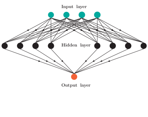
Figure 1: Structure of the artificial neural network used in this work. The number of neurons in the input layer is either 2 or 4. The number of hidden layers is 1 and the number of neurons in the hidden layer is $40$. The number of neurons in the output layer is $1$.

The Bayesian inference is based on Bayes’s theorem, which reads

$$p(\omega|x,t)=\frac{p(\omega)p(x,t|\omega)}{p(x,t)},$$ (3)

where $p(\omega)$ is the prior probability of the parameters of the neural network, $p(x,t|\omega)$ is the likelihood based on the actual data, $p(\omega|x,t)$ is the posterior probability calculated from the prior probability and likelihood, which is used to predict the unknown data, $p(x,t)$ is the marginal likelihood, and $t$ is the set of target data $t_{i}$. Generally speaking, the prior probability encodes our knowledge on the subject under study. In the present case, we assume that the four sets of parameters $\omega=({a,b,c,d})$ are independent of each other and each of them obeys a Gaussian distribution centered around 0 with a width controlled by a hyperparameter. As shown in Ref. Neal (1996), the “gamma” probability distribution is used for the hyperparameter. Similarly, a Gaussian distribution is used for the likelihood in terms of an objective function obtained from a least-squares fit to the training data:

$$p(x,t|\omega)=\exp(-\frac{\chi^{2}(\omega)}{2}),$$ (4)

with

$$\chi^{2}(\omega)=\sum\limits_{i=1}\limits^{N}\left(\frac{t_{i}-f(x_{i},\omega)}{\Delta t_{i}}\right)^{2},$$ (5)

where $N$ is the number of training data. The noise error $\Delta t_{i}$ is an important quantity in the Bayesian method. However, it was usually simplified by taking a fixed value or sampling from a prior distribution Niu and Liang (2018), both of which do not contain much physics. In this work, we use the experimental uncertainties of charge radii as noise errors.

Differently from Ref. Utama et al. (2016b), where only the proton number and mass number of a nucleus are used as inputs to predict its charge radius, we propose to enlarge the number of inputs using feature engineering. Such a method could be referred to as a physically motivated BNN method. It is well known that for many isotopes, such as the calcium and potassium isotopes, charge radii exhibit strong odd-even staggerings. In Refs. An et al. (2020, 2021), such staggerings are related to the so-called Cooper pair condensation or pairing interaction. Inspired by the successful description of calcium An et al. (2020) and potassium An et al. (2021) charge radii, we construct from $Z$ and $N$ two more inputs, i.e., $\delta$ and $P$, which are defined as

$$\delta =\frac{(-1)^{Z}+(-1)^{N}}{2},$$ (6)

$$P =\frac{\nu_{p}\nu_{n}}{\nu_{p}+\nu_{n}}.$$ (7)

The pairing term $\delta$ is related to nuclear pairing effects and the promiscuity factor $P$ Casten et al. (1987); Casten and Zamfir (1996) is related to shell closure effects. In the definition of $P$, $\nu_{p(n)}$ is the difference between the proton (neutron) number of a particular nucleus and the nearest magic number. In this work, the neutron and proton magic numbers are taken as $Z=8,20,28,50,82,126$ and $N=8,20,28,50,82,126,184$ Kirson (2008).

With these two more inputs, the input data for the refined BNN model are $x\equiv(Z,A,\delta,P)$. The target data set $t$ values are $\delta R_{\mathrm{ch}}=R_{\mathrm{exp.}}-R_{\mathrm{NP}}$, i.e., the residuals between experimental data and theoretical predictions of charge radii given by the NP formula.

Unlike other artificial neural networks, the parameters of BNN after training obey a posterior probability. Therefore, the Bayesian predictions for the target data are:

$$\langle f_{n}\rangle=\int f(x_{n},\omega)p(\omega|x,t)d\omega=\frac{1}{K}\sum\limits_{k=1}\limits^{K}f(x_{n},\omega_{k}),$$ (8)

where $\langle f_{n}\rangle$ are the Bayesian predictions, $x_{n}=(Z_{n},A_{n},\delta_{n},P_{n})$ are the input data, $f(x_{n},\omega_{k})$ are the neural network predictions for $\delta R_{\mathrm{ch}}(Z_{n},A_{n})$ for a given set of parameters $\omega_{k}$, and $K$ is the total number of effective samples. In this work, we use the Markov chain Monte Carlo (MCMC) method Neal (1996) to obtain the Bayesian predictions. As long as the MCMC method is used, the marginal likelihood $p(x,t)$ can be ignored. A distinct advantage of BNNs is that they can provide a proper estimate of confidence intervals (CIs) :

$$\Delta=\sqrt{\langle f_{n}^{2}\rangle-\langle f_{n}\rangle^{2}},$$ (9)

where $\langle f_{n}^{2}\rangle$ is obtained following the same procedure as in obtaining $\langle f_{n}\rangle$.

III Results and discussions

In this work, inspired by Refs. An et al. (2020, 2021), we propose a physically motivated BNN model to study nuclear charge radii and to check whether one can reproduce some of the known fine structure and make reliable predictions.

For very light nuclei, because of their small masses and large fluctuations in charge distributions, it is often argued that regarding charge radii as bulk properties is of little meaning Zhang et al. (2002); Sheng et al. (2015). Therefore, we only study those nuclei with $A\geq 40$ and $Z\geq 20$. For the training set, we include the experimental data given in Ref. Angeli and Marinova (2013), which consist of in total 820 data. The more recent experimental data  Day Goodacre et al. (2021); Li et al. (2021), containing 113 data for nuclei with $A\geq 40$ and $Z\geq 20$, are used as the validation set to test the predictive power of our BNN model. The entire set combines the training and validation sets and contains 933 data of nuclear charge radii.

For the sake of easy reference, we use “D4” to denote the model combining the NP formula and the four-input neurons BNN, and “D2” the model combining the NP formula and the two-input neurons BNN. It should be noted that the D2 model is similar to one version of the BNN models of Ref. Utama et al. (2016b). Since the input data and target data have been determined, we can use them to train the BNN. To quantify the extent of the BNN refinement of the NP formula, we compute the RMS deviation between the D4(D2) outputs and experimental data:

$$\sigma_{v}=\sqrt{\frac{1}{N_{v}}\sum\limits_{i=1}\limits^{N_{v}}\left(R_{i}^{(\mathrm{exp.})}-R_{i}^{(\mathrm{theo.})}\right)^{2}}$$ (10)

where $N_{v}$ is the total number of charge radii used in the validation set. The RMS deviations of the training set and the entire set can be calculated in the same way. The corresponding results for the NP formula, D2, and D4 models are displayed in Table 1 for the three data sets, i.e., the training set, the validation set, and the entire set.

Table 1: RMS deviations of charge radii predicted by the NP formula, D2 and D4 models.

	Training set	Validation set	Entire set
$\sigma^{(\mathrm{D2})}~{}(\mathrm{fm})$	0.0161	0.0250	0.0174
$\sigma^{(\mathrm{D4})}~{}(\mathrm{fm})$	0.0143	0.0187	0.0149
$\sigma^{(\mathrm{NP})}~{}(\mathrm{fm})$	0.0394	0.0300	0.0384
$\frac{\sigma^{(\mathrm{NP})}-\sigma^{(\mathrm{D2})}}{\sigma^{(\mathrm{NP})}}$	0.59	0.16	0.55
$\frac{\sigma^{(\mathrm{NP})}-\sigma^{(\mathrm{D4})}}{\sigma^{(\mathrm{NP})}}$	0.64	0.38	0.61

As expected, the D4 model achieves the least RMS deviation for the training set, which is only about 36% of that of the NP formula. Similar improvement is also found for the D2 model. For the validation set, the RMS deviation of the D4 model is only larger by about 31%, while that of the D2 model increases by 55%. Interestingly and somehow unexpectedly, the NP formula describes the validation set better than the training set. We note in passing that, in Ref. Sheng et al. (2015), the modified NP formula which uses $\delta$ and $P$ as two more degrees of freedom achieves an RMS deviation of about 0.0223 fm, which should be compared with 0.0143 fm achieved by our D4 model.

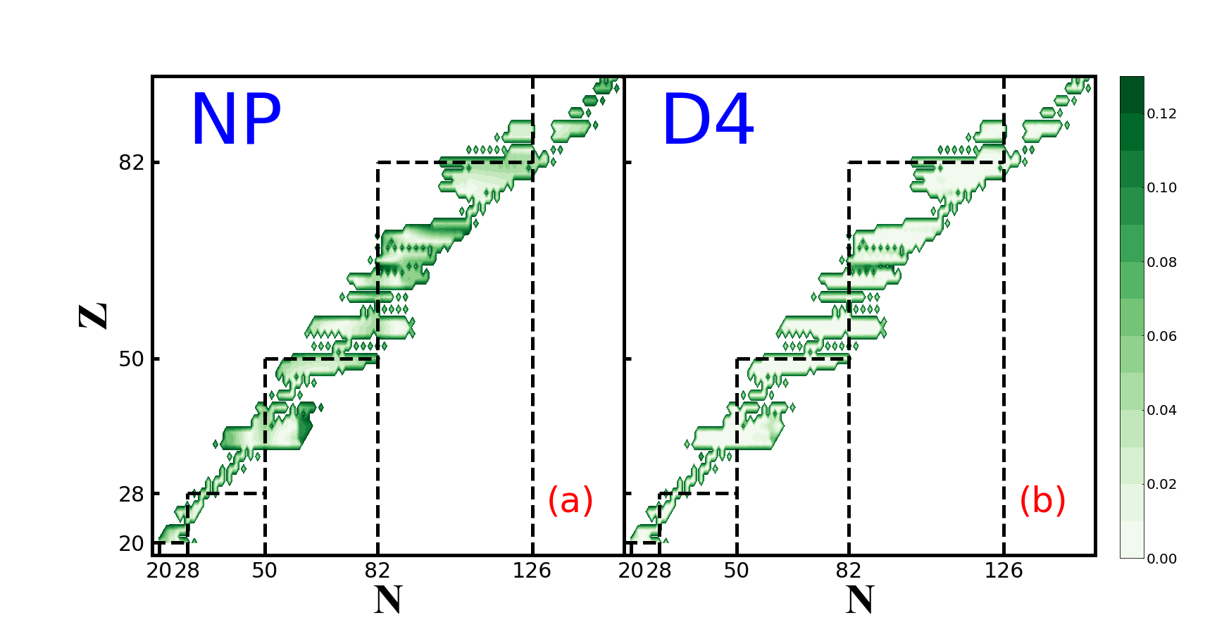
Figure 2: Predictions for the residuals (in units of fm) between the experimental charge radii and the NP formula Nerlo-Pomorska and Pomorski (1994); Bayram et al. (2013) (a) and the D4 model (b) predictions.

For the charge radii of all the nuclei in the entire set, the differences between the theoretical results of the NP formula (the D4 model) and the experimental data are illustrated in Fig. 2. It can be clearly seen that in comparison with the NP formula, the D4 model improves greatly the description of nuclear charge radii.

Although the BNN models with 4 and 2 input neurons seem to describe the training set at a similar level, because of the extra information, “features” ($\delta$ and $P$), contained in the D4 model, it is expected to better describe some fine structure of charge radii, e.g., the odd-even staggerings of charge radii of calcium isotopes. This is indeed the case, as shown in Fig. 3. There are several features about the charge radii of calcium isotopes which pose great challenges to current theoretical models, as summarized in Ref. An et al. (2020). First, the charge radii of ⁴⁰Ca and ⁴⁸Ca are quite close to each other. Second, the odd-even staggerings are very strong in the $A<48$ region and an unexpected large increase is observed in the $A>48$ region Angeli and Marinova (2013); Garcia Ruiz et al. (2016); Miller et al. (2019).

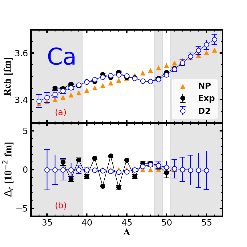
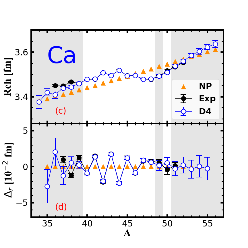
Figure 3: Charge radii (a, c) and $\Delta_{r}$ (b, d) of calcium isotopes predicted by the NP formula Nerlo-Pomorska and Pomorski (1994); Bayram et al. (2013), D2 and D4 models, in comparison with the experimental data Angeli and Marinova (2013); Li et al. (2021). The data in the grey area are predictions, i.e., they are not contained in the training set.

As can be seen from Fig. 3, the dependence of the charge radii on the mass number predicted by the NP formula is almost linear, which fails to give a satisfactory description of the experimental data. With two-input neurons $(Z,A)$, the D2 model describes much better the experimental data but still fails to reproduce the large odd-even staggering, as found by Utama et al. Utama et al. (2016b). With four-input neurons ($Z,A,\delta,P)$, the D4 model describes the data much better, in particular, the odd-even effects of the training set ($40\leq A\leq 48$). Both the D2 and D4 models predict a large increase of the charge radii in the  $A\geq 49$ region. The predicted charge radii for ^49,51,52Ca are in good agreement with the experimental data, which demonstrates the predictive power of artificial neural networks. Nevertheless, we note that the predicted odd-even staggerings by the D4 model for the nuclei with $36\leq A\leq 39$ are a bit stronger than the data.

In the lower panels of Fig. 3, we compare the odd-even staggerings $\Delta_{r}$ defined by

$$\Delta_{r}(N,Z) =\frac{1}{2}\left[R(N-1,Z)-2R(N,Z)+R(N+1,Z)\right],$$ (11)

where $R(N,Z)$ is the RMS charge radius for a nucleus with neutron number $N$ and proton number $Z$. It is clear that neither the NP results nor the D2 results show any odd-even staggerings while the D4 results are in perfect agreement with data. The predictions shown in the grey area, however, suffer from relatively large uncertainties.

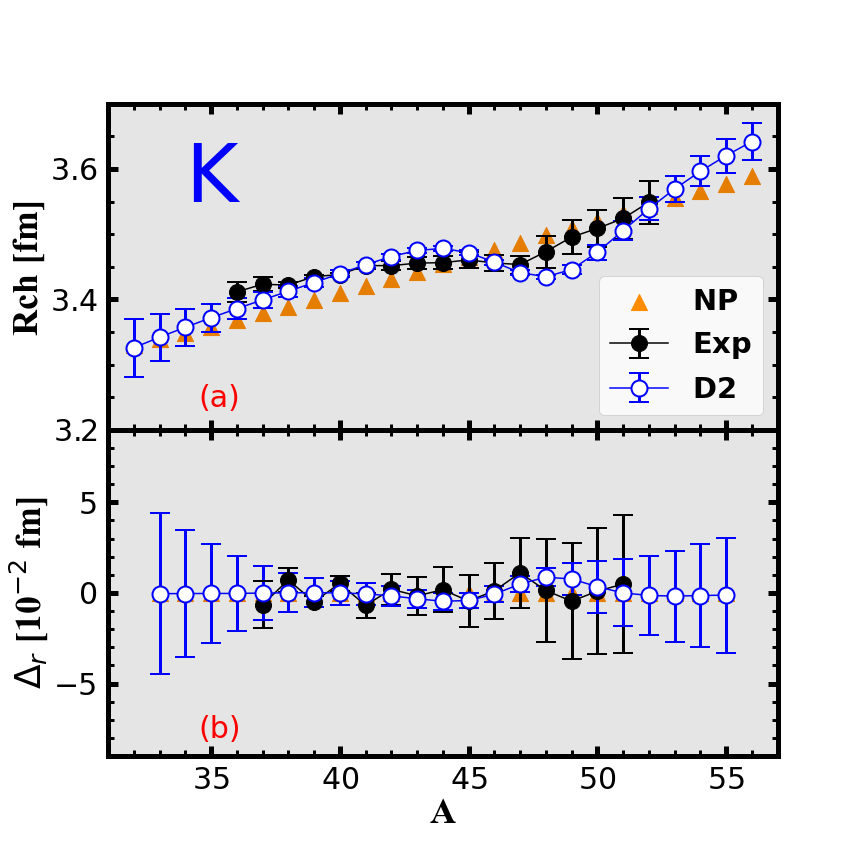
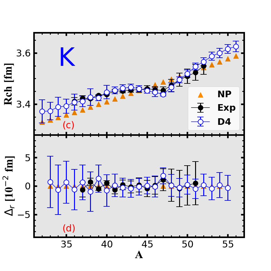
Figure 4: Charge radii (a, c) and $\Delta_{r}$ (b, d) of the potassium isotopes predicted by the NP formula Nerlo-Pomorska and Pomorski (1994); Bayram et al. (2013), D2 and D4 models, in comparison with the experimental data Angeli and Marinova (2013); Koszorús et al. (2021); Li et al. (2021).

It should be noted that the results for calcium isotopes are not completely predictions because the charge radii of some isotopes are used already for training the BNN model. In order to further verify the predictive power of the D2 and D4 models, we calculate the charge radii of potassium isotopes, none of which are used in the training process of our BNN models. The results are shown in Fig. 4. Somehow, surprisingly, the predictions of the D4 model are in very good agreement with the experimental data. It can be seen from Fig. 4 that most experimental data are within the uncertainties of the D4 model, which implies that the charge radii predictions and corresponding uncertainties given by the D4 model are quite reasonable.

Similar to the calcium isotopic chain, neither the NP predictions nor the D2 predictions show any odd-even staggerings while the corresponding results of the D4 model show strong odd-even staggerings, which agree with the experimental data.

Recently, a naive Bayesian probability (NBP) classifier was employed to study nuclear charge radii by fitting to residuals between experimental data and theoretical predictions by the Skyrme-Hartree-Fock-Bogoliubov model and Sheng’s formula Ma et al. (2020). The accuracy of the theoretical predictions for charge radii is improved by about 20% for the validation set after the NBP refinement. However, it cannot reproduce the odd-even staggerings of charge radii of the calcium isotopes.

In Ref. Wu et al. (2020) a feed-forward artificial neural network (ANN) was adopted to directly fit to the experimental data of charge radii. The trained ANN approach reproduces well not only the kinks of charge radii at $N=82$ and $126$ but also the charge radii of calcium isotopes with even neutron number. However, the entire set only contains 347 data, far from enough to make reliable extrapolations for nuclear charge radii throughout the nuclear chart.

IV Summary and outlook

We built a hybrid model which combines a three-parameter parametrization and the flexibility of a Bayesian neural network (BNN) to study nuclear charge radii. We show that with physically motivated features, i.e., pairing and shell effects, one can achieve an unprecedented description of nuclear charge radii. Compared to the three-parameter parametrization, the RMS deviation achieved by the hybrid model is lower by nearly 40%. In particular, the strong odd-even staggerings of calcium isotopes are described very well. In addition, the predictions of the hybrid approach are shown to be in very good agreement with data for potassium isotopes. Another advantage of the hybrid approach is that it can give an estimate of theoretical uncertainties.

The comparison with two- and four-input neurons demonstrated that providing more physical information to the BNN is crucial for the success of the hybrid approach. This should be explored for scenarios where data are limited, which is often the case in nuclear physics.

V Acknowledgments

This work was partly supported by the National Natural Science Foundation of China (NSFC) under Grants No. 11975041, No. 11735003, No. 12105006, and No. 11961141004. R.A. is supported in part by the Reform and Development Project of the Beijing Academy of Science and Technology under Grant No. 13001-2110.

References

- Nortershauser et al. (2009) W. Nortershauser et al., Phys. Rev. Lett. 102, 062503 (2009), arXiv:0809.2607 [nucl-ex] .
- Yang et al. (2016) X. F. Yang et al., Phys. Rev. Lett. 116, 182502 (2016), [Addendum: Phys.Rev.Lett. 116, 219901 (2016)], arXiv:1604.03316 [nucl-ex] .
- Marsh et al. (2018) B. A. Marsh et al., Nature Phys. 14, 1163 (2018).
- de Groote et al. (2020) R. P. de Groote et al., Nature Phys. 16, 620 (2020), arXiv:1911.08765 [nucl-ex] .
- Kreim et al. (2014) K. Kreim et al., Phys. Lett. B 731, 97 (2014), arXiv:1310.5171 [nucl-ex] .
- Gorges et al. (2019) C. Gorges et al., Phys. Rev. Lett. 122, 192502 (2019).
- Angeli and Marinova (2013) I. Angeli and K. P. Marinova, Atom. Data Nucl. Data Tabl. 99, 69 (2013).
- Koszorús et al. (2021) A. Koszorús et al., Nature Phys. 17, 439 (2021), [Erratum: Nature Phys. 17, 539 (2021)], arXiv:2012.01864 [nucl-ex] .
- Day Goodacre et al. (2021) T. Day Goodacre et al., Phys. Rev. Lett. 126, 032502 (2021), arXiv:2012.13802 [nucl-ex] .
- Li et al. (2021) T. Li, Y. Luo, and N. Wang, Atom. Data Nucl. Data Tabl. 140, 101440 (2021).
- Huck et al. (1985) A. Huck, G. Klotz, A. Knipper, C. Miehé, C. Richard-Serre, G. Walter, A. Poves, H. L. Ravn, and G. Marguier, Phys. Rev. C 31, 2226 (1985).
- Wienholtz et al. (2013) F. Wienholtz et al., Nature 498, 346 (2013).
- Rosenbusch et al. (2015) M. Rosenbusch et al., Phys. Rev. Lett. 114, 202501 (2015), arXiv:1506.00520 [nucl-ex] .
- Weizsacker (1935) C. F. V. Weizsacker, Z. Phys. 96, 431 (1935).
- Brown et al. (1984) B. A. Brown, C. R. Bronk, and P. E. Hodgson, J. Phys. G 10, 1683 (1984).
- Nerlo-Pomorska and Pomorski (1994) B. Nerlo-Pomorska and K. Pomorski, Z. Phys. A 348, 169 (1994), arXiv:nucl-th/9401015 .
- Zhang et al. (2002) S. Q. Zhang, J. Meng, S. G. Zhou, and J. Y. Zeng, Eur. Phys. J. A 13, 285 (2002), arXiv:nucl-th/0107040 .
- Wang and Li (2013) N. Wang and T. Li, Phys. Rev. C 88, 011301 (2013), arXiv:1307.2315 [nucl-th] .
- Sheng et al. (2015) Z. Sheng, G. Fan, J. Qian, and J. Hu, Eur. Phys. J. A 51, 40 (2015).
- Geng et al. (2005) L.-S. Geng, H. Toki, and J. Meng, Prog. Theor. Phys. 113, 785 (2005), arXiv:nucl-th/0503086 .
- Goriely et al. (2016) S. Goriely, N. Chamel, and J. M. Pearson, Phys. Rev. C 93, 034337 (2016).
- Peña Arteaga et al. (2016) D. Peña Arteaga, S. Goriely, and N. Chamel, Eur. Phys. J. A 52, 320 (2016).
- Sarriguren (2019) P. Sarriguren, Phys. Rev. C 100, 054306 (2019), arXiv:1911.04313 [nucl-th] .
- Ekström et al. (2015) A. Ekström, G. R. Jansen, K. A. Wendt, G. Hagen, T. Papenbrock, B. D. Carlsson, C. Forssén, M. Hjorth-Jensen, P. Navrátil, and W. Nazarewicz, Phys. Rev. C 91, 051301 (2015), arXiv:1502.04682 [nucl-th] .
- Garcia Ruiz et al. (2016) R. F. Garcia Ruiz et al., Nature Phys. 12, 594 (2016), arXiv:1602.07906 [nucl-ex] .
- An et al. (2020) R. An, L.-S. Geng, and S.-S. Zhang, Phys. Rev. C 102, 024307 (2020), arXiv:2005.00141 [nucl-th] .
- An et al. (2021) R. An, S.-S. Zhang, L.-S. Geng, and F.-S. Zhang, (2021), arXiv:2106.02279 [nucl-th] .
- Carleo et al. (2019) G. Carleo, I. Cirac, K. Cranmer, L. Daudet, M. Schuld, N. Tishby, L. Vogt-Maranto, and L. Zdeborová, Rev. Mod. Phys. 91, 045002 (2019), arXiv:1903.10563 [physics.comp-ph] .
- Bourilkov (2020) D. Bourilkov, Int. J. Mod. Phys. A 34, 1930019 (2020), arXiv:1912.08245 [physics.data-an] .
- Bedolla-Montiel et al. (2021) E. A. Bedolla-Montiel, L. C. Padierna, and R. Castañeda Priego, J. Phys. Condens. Matter 33, 053001 (2021), arXiv:2005.14228 [physics.comp-ph] .
- Bedaque et al. (2021) P. Bedaque et al., Eur. Phys. J. A 57, 100 (2021).
- Hornik et al. (1989) K. Hornik, M. Stinchcombe, and H. White, Neural Networks 2, 359 (1989).
- Utama et al. (2016a) R. Utama, J. Piekarewicz, and H. Prosper, Phys. Rev. C 93, 014311 (2016a), arXiv:1508.06263 [nucl-th] .
- Niu and Liang (2018) Z. M. Niu and H. Z. Liang, Phys. Lett. B 778, 48 (2018), arXiv:1801.04411 [nucl-th] .
- wang et al. (2019) Z.-A. wang, J. Pei, Y. Liu, and Y. Qiang, Phys. Rev. Lett. 123, 122501 (2019), arXiv:1906.04485 [nucl-th] .
- Qiao et al. (2021) C. Y. Qiao, J. C. Pei, Z. A. Wang, Y. Qiang, Y. J. Chen, N. C. Shu, and Z. G. Ge, Phys. Rev. C 103, 034621 (2021), arXiv:2102.09314 [nucl-th] .
- Niu et al. (2019) Z. M. Niu, H. Z. Liang, B. H. Sun, W. H. Long, and Y. F. Niu, Phys. Rev. C 99, 064307 (2019), arXiv:1810.03156 [nucl-th] .
- Alvarez-Ruso et al. (2019) L. Alvarez-Ruso, K. M. Graczyk, and E. Saul-Sala, Phys. Rev. C 99, 025204 (2019), arXiv:1805.00905 [hep-ph] .
- Graczyk and Juszczak (2014) K. M. Graczyk and C. Juszczak, Phys. Rev. C 90, 054334 (2014), arXiv:1408.0150 [hep-ph] .
- Utama et al. (2016b) R. Utama, W.-C. Chen, and J. Piekarewicz, J. Phys. G 43, 114002 (2016b), arXiv:1608.03020 [nucl-th] .
- Wang et al. (2020) R. Wang, Y.-G. Ma, R. Wada, L.-W. Chen, W.-B. He, H.-L. Liu, and K.-J. Sun, Phys. Rev. Res. 2, 043202 (2020), arXiv:2010.15043 [nucl-th] .
- Bayram et al. (2013) T. Bayram, S. Akkoyun, S. O. Kara, and A. Sinan, Acta Phys. Polon. B 44, 1791 (2013).
- Neal (1996) R. M. Neal, Bayesian Learning of Neural Networks (Springer, New York, 1996).
- Casten et al. (1987) R. F. Casten, D. S. Brenner, and P. E. Haustein, Phys. Rev. Lett. 58, 658 (1987).
- Casten and Zamfir (1996) R. F. Casten and N. V. Zamfir, Journal of Physics G: Nuclear and Particle Physics 22, 1521 (1996).
- Kirson (2008) M. W. Kirson, Nuclear Physics A 798, 29 (2008).
- Miller et al. (2019) A. J. Miller, K. Minamisono, A. Klose, D. Garand, C. Kujawa, J. D. Lantis, Y. Liu, B. Maaß, P. F. Mantica, W. Nazarewicz, W. Nrtershuser, S. V. Pineda, P.-G. Reinhard, D. M. Rossi, F. Sommer, C. Sumithrarachchi, A. Teigelhfer, and J. Watkins, Nature Phys. 15, 432 (2019).
- Ma et al. (2020) Y. Ma, C. Su, J. Liu, Z. Ren, C. Xu, and Y. Gao, Phys. Rev. C 101, 014304 (2020).
- Wu et al. (2020) D. Wu, C. L. Bai, H. Sagawa, and H. Q. Zhang, Phys. Rev. C 102, 054323 (2020), arXiv:2006.09677 [nucl-th] .