Superquadric Object Representation for Optimization-based Semantic SLAM

Abstract

Introducing semantically meaningful objects to visual Simultaneous Localization And Mapping (SLAM) has the potential to improve both the accuracy and reliability of pose estimates, especially in challenging scenarios with significant viewpoint and appearance changes. However, how semantic objects should be represented for an efficient inclusion in optimization-based SLAM frameworks is still an open question. sq are an efficient and compact object representation, able to represent most common object types to a high degree, and typically retrieved from 3D point-cloud data. However, accurate 3D point-cloud data might not be available in all applications. Recent advancements in machine learning enabled robust object recognition and semantic mask measurements from camera images under many different appearance conditions. We propose a pipeline to leverage such semantic mask measurements to fit superquadric (SQ) parameters to multi-view camera observations using a multi-stage initialization and optimization procedure. We demonstrate the system’s ability to retrieve randomly generated SQ parameters from multi-view mask observations in preliminary simulation experiments and evaluate different initialization stages and cost functions.

I Introduction

Determining a system’s position in its environment is a crucial task for most mobile robotic applications. Examples include navigation for both wheeled [1] and flying [2] robots, autonomous driving [3], and advanced driving assistance systems (ADAS) for cars and trains [4]. Such positioning is often tackled using visual SLAM techniques [5], achieving robust and accurate state estimation in many applications [6, 7]. However, as most of these systems rely on appearance-based landmarks such as BRISK [8] or ORB [9], their accuracy and reliability tend to decrease in case of significant appearance change of the environment due to variations in illumination or viewpoint. Such changes are especially evident in outdoor applications, in which daytime, weather, and seasonal conditions can influence the appearance significantly [10, 11]. In addition, typical sparse [6, 12] or semi-dense [13] mapping approaches rely on many weak landmarks to enable crucial functionalities such as loop-closure and 6  degrees of freedom (DoF) localization. Therefore, the number of landmarks required for large-scale mapping might invalidate some of the approaches due to memory and bandwidth constraints [3].

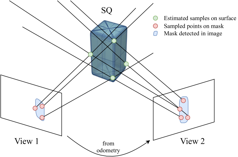
Figure 1: Superquadric parameter fitting from multi-view semantic mask object observations using non-linear optimization.

Over the last decade, deep learning (DL)-based semantic segmentation and object detection algorithms [14, 15, 16] have steadily improved and achieved robust object recognition and instance segmentation covering many different appearance conditions. To leverage these advancements, instead of including generic geometric primitives as landmarks, such as keypoints [6, 12] or lines [17, 18, 19], or utilizing global image descriptors [20, 21, 22] for finding previously visited places, including semantic understanding for SLAM and localization can significantly improve the performance [23, 24, 25, 26]. One way to include semantic understanding is by mapping semantic objects as proposed by Nicholson et al.  [27] or Frey et al.  [28] as strong landmarks. Semantic objects can be consistently detected, are frequent permitting that localization can be achieved often, but are also compact and sparse, enabling large-scale mapping. Furthermore, semantic objects have the potential to be highly descriptive to facilitate localization independent of the current appearance leading to robustness against viewpoint, seasonal, weather, or daytime changes [11].

However, in order to utilize semantic landmarks in state-of-the-art optimization-based SLAM systems [29], on top of finding a distinctive and robust descriptor [24], a compact and computationally efficient representation of the objects has to be found, providing a high representation strength, i.e. is able to accurately represent most common object types.

In this paper, we propose to use SQs as semantic object representations, as a compromise between compactness and representation strength. To enable the usage of SQs in mapping tasks without being dependent on depth data, we propose to retrieve SQ parameters from multi-view semantic mask observations as shown in Figure 1. Furthermore, we propose the adaption of an analytic cost function of the fitting quality to multi-view mask observations for an efficient implementation of SQs in optimization-based SLAM frameworks. We evaluate the retrieval quality and multiple initialization techniques on randomly generated SQs in simulation, demonstrating the ability to successfully retrieve SQ parameters with high fitting accuracy.

II Related Work

Semantic objects can be mathematically represented in many different ways, typically as a trade-off between parametrization complexity and representation strength. Simple 3D point representations as mapped in [30, 28] consist of three position parameters, equivalent to standard keypoints. This benefits from an easy integration of well-known re-projection cost functions, but especially objects with larger sizes or non-spherical shapes cannot be represented accurately. This problem can be addressed by including size parameters resulting in cubes [31], spheres [32], or ellipsoids/quadrics [33, 27]. However, if the mapped object has a different shape than modeled by the representation, inaccuracies and wrong scene understandings might result. In contrast, complex dense representations such as Euclidean signed distance fields [34, 35, 36, 37] result in measurement functions that are tricky to include in optimization frameworks, rely on a high dimensional parametrization, and require many observations for a good shape estimation. Ultimately, the object can be represented by high-accuracy 3D models [38, 39], which, however, requires a good database of the expected objects in order to work reliably.

SQs as initially introduced to the computer vision community by Barr et al.  [40] are an extension to standard quadrics and can represent a wide range of common convex object types with only 11 parameters. The retrieval of SQ parameters is extensively researched and typically solved by fitting 3D point-cloud data using non-linear least-squares optimization [41, 42, 43, 44, 45, 46]. Also, DL-based retrieval from 3D point-cloud data was recently proposed [47]. In contrast, in this work, we focus on retrieving SQ parameters from multi-view camera observations to be independent on accurate range data, which might not be available, especially in outdoor environments.

Most object-based SLAM frameworks, which do not depend on depth data, retrieve and optimize object and camera pose parameters from 2D bounding box observations [27, 33, 31]. However, such camera-frame axis-aligned bounding boxes are not able to accurately represent objects which are not aligned to the camera view, especially if the objects have non-equal dimensions. In contrast, recent semantic instance segmentation networks [14, 15] achieve high accuracy in not only detecting the objects but also capturing their shape in the current camera view.

How such semantic mask observations can be utilized to efficiently retrieve and optimize SQ parameters and leverage the additional shape information is an open question that we aim to address in this paper.

III Superquadric Fitting for Semantic Measurements

This section gives an overview of SQs, introduces our pipeline to retrieve and optimize SQ parameters based on semantic mask observations, and describes an analytic cost function that approximates the fit of the observation data with the SQ model.

III-A Notation

In this document, we denote scalars as $a$, vector-valued variables as $\mathbf{a}$, matrices as $\mathrm{A}$, and a set of variables as $\mathcal{A}$. 3D points are denoted in homogeneous coordinates as $\prescript{}{A}{\mathbf{t}}\in\mathbb{R}^{4}$ represented in the coordinate frame $A$, and a set of 3D points as $\prescript{}{A}{\mathcal{T}}$. Furthermore, $\mathrm{T}^{B}_{A}\in\mathbb{R}^{4\times 4}$ indicates a homogeneous coordinate transformation to transform a point described in frame $B$ into frame $A$, i.e. $\prescript{}{A}{\mathbf{t}}=\mathrm{T}^{B}_{A}\cdot\prescript{}{B}{\mathbf{t}}$. Poses of both cameras and SQs are denoted by a position $\prescript{}{W}{\mathbf{p}}\in\mathbb{R}^{3}$ and an orientation $\prescript{}{W}{\mathbf{r}}\in\mathbb{R}^{3}$ using Euler angles with respect to the world coordinate frame $W$. A set of poses is denoted by $\mathcal{P}$.

III-B Superquadrics

sq are mathematical shapes fully describable by a compact number of parameters. They extend standard quadrics by incorporating additional shape parameters to define the objects’ roundness. A point on the surface of a SQ $\prescript{}{SQ}{\mathbf{t}}=\left[t_{x},t_{y},t_{z}\right]$ is found by its direct formulation [41]

$$\prescript{}{SQ}{\mathbf{t}}=\left[\begin{array}[]{c}a_{x}\cdot\cos(\eta)^{\varepsilon_{1}}\cdot\cos(\omega)^{\varepsilon_{2}}\\ a_{y}\cdot\cos(\eta)^{\varepsilon_{1}}\cdot\sin(\omega)^{\varepsilon_{2}}\\ a_{z}\cdot\sin(\eta)^{\varepsilon_{1}}\end{array}\right],$$ (1)

where $a_{\bullet}$ are the size parameters in each dimension, $\varepsilon_{\bullet}$ are the two shape parameters, and $-\frac{\pi}{2}\leq\eta\leq\frac{\pi}{2}$ and $-\pi\leq\omega\leq\pi$ are iteration variables. Using Equation (1), points on the SQ surface can be sampled and projected to the camera view to evaluate the quality of fit between the projected SQ and the mask observations by evaluating the reprojection intersection over union (R-IOU).

However, in this work, primarily the implicit formulation of SQs [48] is of interest given by

$$F\left(\prescript{}{SQ}{\mathbf{t}}\right)=\left(\left(\frac{t_{x}}{a_{x}}\right)^{\frac{2}{\varepsilon_{2}}}+\left(\frac{t_{y}}{a_{y}}\right)^{\frac{2}{\varepsilon_{2}}}\right)^{\frac{\varepsilon_{2}}{\varepsilon_{1}}}+\left(\frac{t_{z}}{a_{z}}\right)^{\frac{2}{\varepsilon_{1}}}=1,$$ (2)

where $\prescript{}{SQ}{\mathbf{t}}=\left[t_{x},t_{y},t_{z}\right]$ is a point on the SQ surface in SQ coordinates.

In addition to the size $\mathbf{a}$ and shape $\mathbf{\varepsilon}$, a general SQ in 3D space is defined by its position $\prescript{}{W}{\mathbf{p}_{SQ}}\in\mathbb{R}^{3}$ and orientation $\prescript{}{W}{\mathbf{r}_{SQ}}\in\mathbb{R}^{3}$ in world coordinates $W$, forming a transformation $\mathrm{T}_{SQ}^{W}$ from world to SQ coordinates. In total, a SQ is defined by the parameters $\mathbf{\xi}=\left[\mathbf{a},\mathbf{\varepsilon},\mathbf{p},\mathbf{r}\right]\in\mathbb{R}^{11}$. The implicit formulation in Equation (2) directly provides an insight into whether a point $\prescript{}{SQ}{\mathbf{t}}$ lies on the surface $F\left(\prescript{}{SQ}{\mathbf{t}}\right)=1$, is located outside of the SQ $F\left(\prescript{}{SQ}{\mathbf{t}}\right)>1$, or on its inside $F\left(\prescript{}{SQ}{\mathbf{t}}\right)<1$.

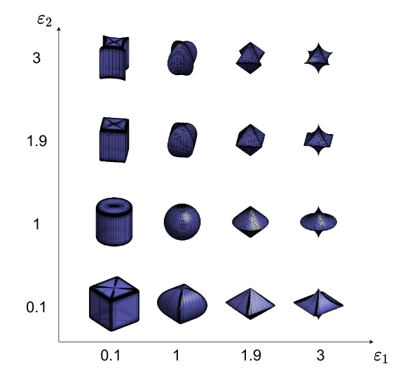
Figure 2: SQs with unit size ($\mathbf{a}=\mathbf{1}$). The shape parameters $\mathbf{\varepsilon}$ define the edginess of the final object. To keep the optimization stable [46] and consider only convex shapes, only shape parameters $0.1\leq\mathbf{\varepsilon}\leq 1.9$ are considered in this work.

Depending on the coupling of the shape parameters $\varepsilon$, SQs represent cubic objects, spheres, and ellipsoids, up to convex shapes and everything in between, such as cylinders. Figure 2 shows an overview of the achievable shapes with different shape parameters. In the case where both shape parameters are $\varepsilon=\mathbf{1}$, the SQ becomes equivalent to a standard quadric. In this work, to minimize numerical problems and keep the optimization as stable as possible [46], we only consider convex objects with shape parameters

$$0.1\leq\mathbf{\varepsilon}\leq 1.9.$$ (3)

III-C Optimizing R-IOU

To achieve our goal of SQ parameter retrieval given observation data, in our case multi-view semantic mask observations $\mathcal{O}$, we formulate the following optimization problem

$$\xi_{opt}=\operatorname*{arg\,min}_{\xi}{\sum_{p=1}^{P}}G_{1}\left(\xi,\mathcal{O},\mathcal{P}\right)^{2},$$ (4)

where $\mathcal{P}$ is the set of $P$ poses that observe the SQ. This optimization problem can be solved using the non-linear least-squares Levenberg-Marquardt optimization algorithm [49, 50]. The cost function $G_{1}$ is formed by

$$G_{1}=1-\acs{riou}\left(\xi,\mathcal{O},\mathcal{P}\right),$$ (5)

where the R-IOU is evaluated by comparing the re-projected estimated SQ $\xi$ according to Equation (1) and camera poses $\mathcal{P}$ with the semantic mask observation $o\in\mathcal{O}$. As the mask observation is likely to be non-parametric, the 2D intersection over union (IOU) evaluation is based on polyshapes [51]. This drastically complicates the retrieval of analytic Jacobians for the cost function. Therefore, numerical derivations using finite differences are used for the optimization of $G_{1}$. The state constraints $\xi_{th}$ mentioned in Equation (3), as well as the condition of a non-negative and non-vanishing size $\mathbf{a}\geq 0.1$, are included in the optimization as a soft constraint penalty

$$G_{2} =G_{1}+c_{p}\cdot\sum_{i=1}^{K}\rho_{i},$$ (6)

$$\rho_{i} =\begin{dcases}|\xi^{i}-\xi_{th}^{i}|&\text{if}\;\xi^{i}<\xi_{th,l}^{i}\;\text{or}\;\xi^{i}>\xi_{th,u}^{i}\\ 0&\text{otherwise},\end{dcases}$$

where $c_{p}$ is a heuristic cost penalty, $\xi^{i}$ is one of the state variables, $K$ is the state size, and $\xi_{th,l}$ and $\xi_{th,u}$ are the lower and upper thresholds, respectively.

III-D Analytic cost function and optimization problem

To effectively use SQ-landmarks in the optimization of a factor-graph-based SLAM setup, an efficient and derivable formulation of the R-IOU is required. The radial distance $G_{3}$ was proposed by Zhang et al.  [43] to represent the error of a SQ fitted to a 3D point cloud (PC). $G_{3}$ is the distance from any given point ${}_{W}\mathbf{t}$ to the surface of a SQ $\xi$ and is calculated as

$$G_{3}\left(\mathbf{\xi},\prescript{}{SQ}{\mathbf{t}}\right)=||\prescript{}{SQ}{\mathbf{t}}||\left[F(\prescript{}{SQ}{\mathbf{t}})^{-\frac{\varepsilon_{1}}{2}}-1\right],$$ (7)

where $\prescript{}{SQ}{\mathbf{t}}=\mathrm{T}_{SQ}^{W}\cdot\prescript{}{W}{\mathbf{t}}$ is a 3D point transformed into SQ coordinates and $F$ is the implicit SQ formulation in Equation (2). The main objective for SQ fitting, as shown in e.g. [42, 46, 43, 44, 45] is then to minimize $G_{3}$ for a number $N$ of 3D point observations such that

$$\xi_{opt}=\operatorname*{arg\,min}_{\xi}{\sum_{n=1}^{N}}G_{3}\left(\xi,\mathrm{T}_{SQ}^{W}\cdot\prescript{}{W}{\mathbf{t}_{n}}\right)^{2}.$$ (8)

However, our approach aims to recover SQ shapes from multi-view camera mask observations without being dependent on accurate depth data. Therefore, such mask observations are randomly sampled to obtain $N$ observation samples $\mathbf{s}=\left[s_{x},s_{y}\right]\in\mathcal{S}_{o}$ per object observation $o\in\mathcal{O}$. Finally, $\mathbf{s}$ can be back-projected from the estimated camera pose $\mathrm{T}_{W}^{C}\left(\mathbf{p}_{C},\mathbf{r}_{C}\right)\in\mathcal{P}$, where $\mathbf{p}_{C}$ and $\mathbf{r}_{C}$ are the camera position and orientation, respectively,

$$\begin{split}\prescript{}{W}{\mathbf{t}}&={T}_{W}^{C}\cdot Bp(\mathbf{s},d)\\ &=\mathrm{T}_{W}^{C}\cdot\left[d\cdot\left[(s_{x}-\kappa_{x})/f_{x},(s_{y}-\kappa_{y})/f_{y},1\right]^{\top}\right],\end{split}$$ (9)

using known camera intrinsics, where $\kappa_{\bullet}$ are the camera centers and $f_{\bullet}$ are the focal lengths. The parameters $d\in\mathcal{D}$ are unknown depth parameters and can either be per camera view termed combined depth, or per single observation sample $\mathbf{s}$ termed separate depth. Hence, the optimization problem of Equation (8) becomes

$$\left[\xi_{opt},\mathcal{D}_{opt}\right]=\operatorname*{arg\,min}_{\xi,\mathcal{D}}{\sum_{p=1}^{P}\sum_{n=1}^{N}}G_{4}\left(\xi,\mathcal{S}_{p,n},\mathcal{P}_{p},\mathcal{D}_{p}\right)^{2}.$$ (10)

$G_{4}$ cannot penalty SQs that are larger than what is represented by the mask observations, as long as the sample points $\mathcal{S}$ are on its surface. Together with the variable depths $d\in\mathcal{D}$, this results in an unconstrained size of the SQ which is typically heavily overestimated. To circumvent this issue, an additional factor is introduced to the cost function to retrieve the minimal size SQ, which still agrees to the mask observation data

$$G_{5}=\left(a_{x}\cdot a_{y}\cdot a_{z}+1\right)\cdot G_{4}.$$ (11)

For all analytic cost functions $G_{3}-G_{5}$, the same constraint violation penalty introduced in Equation (6) is applied.

III-E Multi-stage optimization

Using the Levenberg-Marquardt algorithm to optimize $G_{5}$, we discovered that the optimization is fragile and subject to deep local minima. Therefore, to achieve high robustness, reliability, and accuracy, a good initialization of all SQ parameters close to the global minimum is required. We propose to use the following multi-stage initialization and optimization procedure to achieve good convergence of the parameters:

III-E1 Triangulation and combined depth

Triangulation is a widespread method typically used to initialize 3D keypoint positions from multi-camera observations. We use linear triangulation to initialize the position of the SQ $\prescript{}{W}{\mathbf{\hat{p}}}_{SQ}$ based on back-projection of the centroid $\mathbf{c}_{i}$ of the mask observations

$$\prescript{}{W}{\mathbf{v}}_{i}=\mathrm{R}^{C_{i}}_{W}\cdot Bp(\mathbf{c}_{i},1)\quad\forall\,i\in\mathcal{P},$$ (12)

$$\mathrm{A}=\left[\begin{array}[]{cccc}\mathbb{1}&-\prescript{}{W}{\mathbf{v}_{1}}&\mathbb{0}&\mathbb{0}\\ &\vdots&\\ \mathbb{1}&\mathbb{0}&-\prescript{}{W}{\mathbf{v}_{i}}&\mathbb{0}\\ &\vdots&\\ \mathbb{1}&\mathbb{0}&\mathbb{0}&-\prescript{}{W}{\mathbf{v}_{P}}\end{array}\right],\,b=\left[\begin{array}[]{c}\prescript{}{W}{\mathbf{p}_{C_{1}}}\\ \vdots\\ \prescript{}{W}{\mathbf{p}_{C_{i}}}\\ \vdots\\ \prescript{}{W}{\mathbf{p}_{C_{P}}}\end{array}\right],$$ (13)

where $\prescript{}{W}{\mathbf{v}_{i}}$ is the $i$th centroid’s bearing vector, $\mathrm{R}^{C_{i}}_{W}$ is the rotation part of $\mathrm{T}^{C_{i}}_{W}$, $Bp$ is the back-projection function in Equation (9), $\mathbb{1}$ is the identity matrix, and $P$ is the number of observations and corresponding poses. The triangulation point $\prescript{}{W}{\mathbf{\hat{p}}}_{SQ}$ is then extracted from the first three elements of $\mathbf{x}$ obtained by solving $\mathrm{A}\cdot\mathbf{x}=\mathbf{b}$ using QR-decomposition.

Furthermore, a rough prior for the depth parameter $d_{i}\in\mathcal{D}$ utilized in the back-projection in Equation (9) for each camera view, i.e. a unified depth for a mask observation, is obtained by solving

$$\prescript{}{W}{\mathbf{p}}_{C_{i}}+d_{i}\cdot\prescript{}{W}{\mathbf{v}_{i}}=\prescript{}{W}{\mathbf{\hat{p}}}_{SQ}.$$ (14)

III-E2 Orientation, size, and separate depth

To get a prior and initialization on the remaining parameters of a quadric and good estimates for a per-sample depth, we utilize a principal component analysis (PCA)-like initialization procedure.

The main idea is to find the most prominent directions and corresponding sizes in a PC built by back-projecting the mask observation samples $\mathcal{S}$ with the depth prior $\mathcal{D}$ estimated in the previous triangulation step. This is achieved by determining the principle components of the PC using PCA [52] providing a rotation matrix corresponding to the most prominent direction, i.e. the orientation of the PC, which is used as prior for the orientation of the SQ. Evaluating the boundaries of the rotated PC directly serves as a prior for the object size.

Finally, a per-sample depth is obtained by optimizing $G_{4}$ with respect to only the depth parameter using the initialized fixed SQ, in this case a quadric with $\varepsilon=\mathbf{1}$, position determined from triangulation, and orientation and size estimated using the procedure described above.

The overall algorithm to initialize orientation, size, and separate depth is summarized in Algorithm 1.

1:procedure PCAI($\mathcal{S},\mathcal{D},\mathcal{P},\prescript{}{W}{\mathbf{p}_{SQ}}$)

2: 

3:Phase 1 - Back-project semantic measurement samples

4: 

5:   $\prescript{}{W}{\mathcal{T}}\leftarrow$ Ø$\triangleright$ Initialize points in world coordinates

6:   for all $o\in\mathcal{O}$ do

7:      $d\leftarrow\mathcal{D}_{o}$ $\triangleright$ Same depth for every sample

8:      $\mathrm{T}_{W}^{C}\leftarrow\mathcal{P}_{o}$

9:      for all $\mathbf{s}\in\mathcal{S}_{o}$ do

10:         Add $\mathrm{T}_{W}^{C}\cdot Bp(\mathbf{s},d)$ to $\prescript{}{W}{\mathcal{T}}$ $\triangleright$ Using Eq. (9)          

11:   $N\leftarrow\text{number of samples in }\prescript{}{W}{\mathcal{T}}$

12: 

13:Phase 2 - PCA

14: 

15:   $\mathrm{A}\leftarrow\text{zeroMean}(\prescript{}{W}{\mathcal{T}})$

16:   $\mathrm{U}\cdot\mathrm{\Sigma}\cdot\mathrm{V}^{*}=\operatorname{SVD}(\frac{\mathrm{A}}{\sqrt{N-1}})$

17:   $\mathrm{S}\leftarrow\mathrm{V}^{*\top}\cdot\mathrm{A}$ $\triangleright$ Rotated samples

18: 

19:Phase 3 - Extract size, orientation, and depths

20: 

21:   $\mathbf{a}\leftarrow\frac{\max{\mathrm{S}}-\min{\mathrm{S}}}{2}$

22:   $\prescript{}{W}{\mathbf{r}_{SQ}}\leftarrow\operatorname{Euler}(\mathrm{V^{*}})$ $\triangleright$ Convert $\mathbf{\mathrm{V}^{*}}$ to Euler angles

23:   $\mathbf{\xi}=\left[\mathbf{a},\mathbf{1},\prescript{}{W}{\mathbf{p}_{SQ}},\prescript{}{W}{\mathbf{r}_{SQ}}\right]$ $\triangleright$ Quadric with $\varepsilon=\mathbf{1}$

24:   for all $o\in\mathcal{O}$ do

25:      for all $\mathbf{s}_{i}\in\mathcal{S}_{o}$ do

26:         $d_{i}\in\mathcal{D}\leftarrow\operatorname*{arg\,min}_{d}{G_{4}\left(\mathbf{\xi},\mathbf{s}_{i},\mathcal{P}_{o},d\right)^{2}}$          

27:   return $\left[\mathbf{\xi},\mathcal{D}\right]$

Algorithm 1 PCA initialization

III-E3 Optimization

The final step of SQ retrieval is to use the optimization introduced in Equation (4) or (10) initialized using the previous stages. Multiple optimization setups are used, concatenated, and compared:

1. Numeric optimization of all SQ parameters using $G_{2}$ in Equation (4).

2. Numeric optimization with $G_{2}$ of only quadric parameters, fixing $\varepsilon=\mathbf{1}$.

3. Optimization of quadric parameters, fixing $\varepsilon=\mathbf{1}$ and using combined depths, i.e. only optimizing one depth parameter per view, using $G_{5}$ in Equation (10).

4. Optimizing only quadric parameters as in option C), but optimizing a separate depth variable per sample.

5. Optimizing all SQ parameters with separate depth variables using $G_{5}$ in Equation (10). This corresponds to the same potential outcome as in option A), but uses the analytic cost function $G_{5}$ instead of $G_{2}$.

6. Using the numeric cost function $G_{2}$ for optimizing the shape parameters $\varepsilon$ while fixing all other parameters.

IV Experiments

To evaluate the proposed method’s applicability, performance, and accuracy, we conducted different preliminary experiments in a simulation environment.

IV-A Simulation and experimental setup

Our simulator implemented in MATLAB is able to create random ground truth (GT) SQ objects, create pinhole camera trajectories that observe the object, and calculate the semantic mask observations by projecting the SQ to the camera view. The projected SQ measurements are then randomly sampled, as described in Section III-D, to obtain the set of semantic mask observations $\mathcal{O}$. Like this, we can create a realistic scenario of a robotic agent or person equipped with a camera moving around an area while observing an object. A main benefit of using the simulation environment is the decoupling of our evaluation from uncertainties and challenges typically introduced with other computer vision tasks, such as pose estimation, semantic object detection and instance segmentation, and multi-view data association, which allows for an independent investigation of the proposed method.

For the preliminary results in Section IV-B, we utilized three camera views arranged in a circle around the object (see Figure 4). To evaluate the ability and robustness of fitting a SQ to multi-view mask observations, a permutation experiment is conducted by generating GT SQs with random parameters within a given working area to ensure valid observations from the camera views. The most important parameters of the simulation environment and permutation experiment are summarized in Table I. Finally, the camera poses and mask observations are utilized in the fitting procedure introduced in Section III with different settings and concatenations to retrieve SQs that can be compared to the GT. The numeric cost functions in Stages 3A, 3B, and 3F utilize the convex hull of the semantic measurement samples $\mathcal{O}$ as an observation. For the non-linear optimization detailed in Stage 3, we used the Levenberg-Marquart implementation provided by the lsqcurvefit function.

The evaluation metrics are (1) the IOU of the estimated 3D SQ and the GT SQ, (2) the mean 2D R-IOU of the re-projected estimated SQ and re-projected GT SQ on all utilized observer camera views (R-IOU), and (3) the mean 2D R-IOU of the estimated SQ and the convex hull of the semantic measurements samples $\mathcal{O}$ as obtained with the procedure described in Section III-D, termed R-IOU-M. In addition, we also define a success rate $\sigma$. A fit is deemed successful if the estimated and GT SQ are overlapping, i.e. $\text{IOU}>0$.

As the optimization is based on mask observations, the IOU might be misleading as it depends on the observability of the different parameters. In contrast, the R-IOU more accurately represents the fit quality of the observation data.

TABLE I: Overview of the simulation environment parameters

Camera resolution	$640\times 480\,\mathrm{px}$
Camera focal length	$400\times 300\,\mathrm{px}$
Camera image center	$320\times 240\,\mathrm{px}$
Camera trajectory circle radius	$10\,\mathrm{m}$
Camera views	$3$
Number of permutations	$100$
Samples per observation $N$	$100$
Constraint violation penalty $G_{2}$	$c_{p}=1$
Constraint violation penalty $G_{3}$ to $G_{5}$	$c_{p}=100$
SQ size range	$\mathbf{a}\in\{0.1,5\}\,\mathrm{m}$
SQ position range	$\prescript{}{W}{\mathbf{p}}\in\{-5,5\}\,\mathrm{m}$
SQ orientation range	$\prescript{}{W}{\mathbf{r}}\in\{-\pi,\pi\}\,\mathrm{rad}$
SQ shape range	$\mathbf{\varepsilon}\in\{0.1,1.9\}$

IV-B Results and Discussion

TABLE II: Overview of the achievable accuracy and robustness in the permutation experiment using different stage concatenations fitting 100 random SQs using multi-view mask observations. The values correspond to the final result after the last stage. M: Median, A: Average, StD: Standard deviation

	IOU			R-IOU			R-IOU-M			Time${}^{\text{a}}$ $[\mathrm{s}]$			$\sigma$
Stages	M	A	Std	M	A	Std	M	A	Std	M	A	Std
3A	0.401	0.370	0.351	0.726	0.489	0.385	0.770	0.523	0.417	2.669	6.351	8.990	$66\,\mathrm{\%}$
3B	0.282	0.363	0.336	0.745	0.509	0.371	0.773	0.537	0.396	1.963	3.138	3.807	$67\,\mathrm{\%}$
1$\rightarrow\;$3A	0.686	0.636	0.185	0.846	0.808	0.104	0.920	0.872	0.117	6.607	9.518	8.446	$100\,\mathrm{\%}$
1$\rightarrow\;$2$\rightarrow\;$3A	0.741	0.688	0.174	0.852	0.841	0.073	0.919	0.906	0.082	5.183	7.231	5.926	$100\,\mathrm{\%}$
1$\rightarrow\;$2$\rightarrow\;$3B	0.739	0.694	0.146	0.835	0.836	0.025	0.897	0.895	0.029	3.184	4.630	3.682	$100\,\mathrm{\%}$
3E	0.000	0.000	0.001	0.007	0.015	0.021	0.007	0.015	0.021	1.075	1.066	0.277	$18\,\mathrm{\%}$
1$\rightarrow\;$3E	0.009	0.044	0.071	0.089	0.137	0.142	0.103	0.154	0.156	1.009	1.018	0.263	$100\,\mathrm{\%}$
1$\rightarrow\;$2$\rightarrow\;$3C	0.012	0.061	0.103	0.107	0.153	0.141	0.123	0.175	0.158	0.514	1.045	1.267	$100\,\mathrm{\%}$
1$\rightarrow\;$2$\rightarrow\;$3D	0.516	0.488	0.261	0.766	0.730	0.159	0.668	0.650	0.134	0.876	1.396	3.097	$100\,\mathrm{\%}$
1$\rightarrow\;$2$\rightarrow\;$3E	0.435	0.427	0.198	0.641	0.635	0.143	0.649	0.624	0.130	1.350	1.855	5.862	$100\,\mathrm{\%}$
1$\rightarrow\;$2$\rightarrow\;$3D$\rightarrow\;$3E	0.516	0.488	0.261	0.766	0.730	0.159	0.668	0.650	0.134	0.877	1.426	3.131	$100\,\mathrm{\%}$
1$\rightarrow\;$2$\rightarrow\;$3D$\rightarrow\;$3A	0.760	0.694	0.169	0.856	0.847	0.059	0.924	0.910	0.069	5.688	7.765	6.050	$100\,\mathrm{\%}$
1$\rightarrow\;$2$\rightarrow\;$3D$\rightarrow\;$3F	0.622	0.536	0.234	0.784	0.749	0.126	0.793	0.759	0.127	1.895	2.837	5.706	$100\,\mathrm{\%}$

${}^{\text{a}}$ The system is tested on an AMD Ryzen 5 1600 $3.2\,\mathrm{GHz}$, 12 threads, $16\,\mathrm{GB}$ RAM running MATLAB R2020a.

The optimization of SQ parameters to fit multi-view mask observations by directly maximizing the R-IOU, as described in Section III-C and Stages 3A and 3B, is challenging as there are zero gradients if there is no overlap between the initialized SQ and the mask observation. This results in a low success rate and demands for a good initialization.

This is even more drastic when using the analytic cost functions described in Stages 3C to 3E for the direct optimization of SQ parameters, which highly depends on a good initialization and often results in local minima and a bad fit.

We, therefore, propose different concatenations of the stages introduced in Section III-E to achieve convergence. Table II shows an overview of the different fitting setups tested.

Using the stage concatenation 1$\rightarrow\;$2$\rightarrow\;$3D$\rightarrow\;$3A achieves the best quality as it optimally utilizes all available information, i.e. the semantic mask measurements, and is well initialized. However, the optimization is relatively slow as it depends on finite differences for the optimization. Note, that full parallelization is utilized for finite differences while the analytic Jacobians are evaluated on a single CPU thread.

Optimizing all SQ parameters instead of only quadrics only gives a slight advantage. However, this evaluation is biased as the permutation uniformly samples all possible $\varepsilon$, leading to non-extreme SQs in many cases. When specifically considering more extreme SQs, e.g. only if one of the $\varepsilon<0.15$ or $\varepsilon>1.85$, the performance improvement becomes more evident, i.e. 0.695 vs. 0.732, 0.819 vs. 0.851, and 0.875 vs. 0.930 for the median IOU, R-IOU and R-IOU-M for the combinations 1$\rightarrow\;$2$\rightarrow\;$3B and 1$\rightarrow\;$2$\rightarrow\;$3A, respectively.

Using the analytic cost function $G_{5}$ in 1$\rightarrow\;$2$\rightarrow\;$3D shows a good performance in retrieving quadric parameters with a lower computational cost. However, adding the shape parameters in the optimization in Stage 3E does not significantly improve the results. It may even lead to the creation and convergence into new local minima.

A compromise between shape recovery and higher computational performance is achieved with the stage combination 1$\rightarrow\;$2$\rightarrow\;$3D$\rightarrow\;$3F. Furthermore, initializing Stage 3A with 3D in the sequence 1$\rightarrow\;$2$\rightarrow\;$3D$\rightarrow\;$3A leads to a slight boost in computational performance for the final step, but considering the time required for Stage 3D, which runs on a single thread, a more in-depth analysis is required to justify the computational advantage.

Finally, utilizing a single depth per camera view as proposed in Stage 3C did not work well as the optimization typically converges to a thin camera-aligned quadric. This is especially evident in larger SQs. The main reason for this is the limited flexibility in depth estimation.

Figure 3 shows the permutation summary, and Figure 4 shows an example of a typical random SQ fitted from multi-view mask observations using the stage combination 1$\rightarrow\;$2$\rightarrow\;$3D$\rightarrow\;$3A. Both figures showcase the individual contribution of each stage to the final solution. Stage 1 of the initialization, i.e triangulation, correctly recovers the average position and predicts the approximate depth parameters for each camera view. However, as expected, the shape, size, and orientation are far different from the GT. After the second stage of the optimization, the PCA initialization, orientation and size are initialized, and the depth samples are fitted to the surface of the prior quadric. The parameters of the quadric can further be refined by performing separate depth parameter optimization in Stage 3D. The size, orientation, and position of the object are correctly recovered from only three camera observations. Finally, Stage 3A achieves an accurate fit to the GT SQ with a large IOU and R-IOU.

Typically, the optimized SQ size and edginess parameters are slightly underestimated, mainly due to the chosen random sampling procedure of the semantic mask observations. This results in under-represented extremes of the contour of the re-projected SQ and is one of the reasons why SQ are only performing marginally better than quadrics in our experiments. An adaptive sampling procedure focusing on the most informative samples might help mitigate the underestimation and make the difference between quadric and SQ parameter fitting clearer.

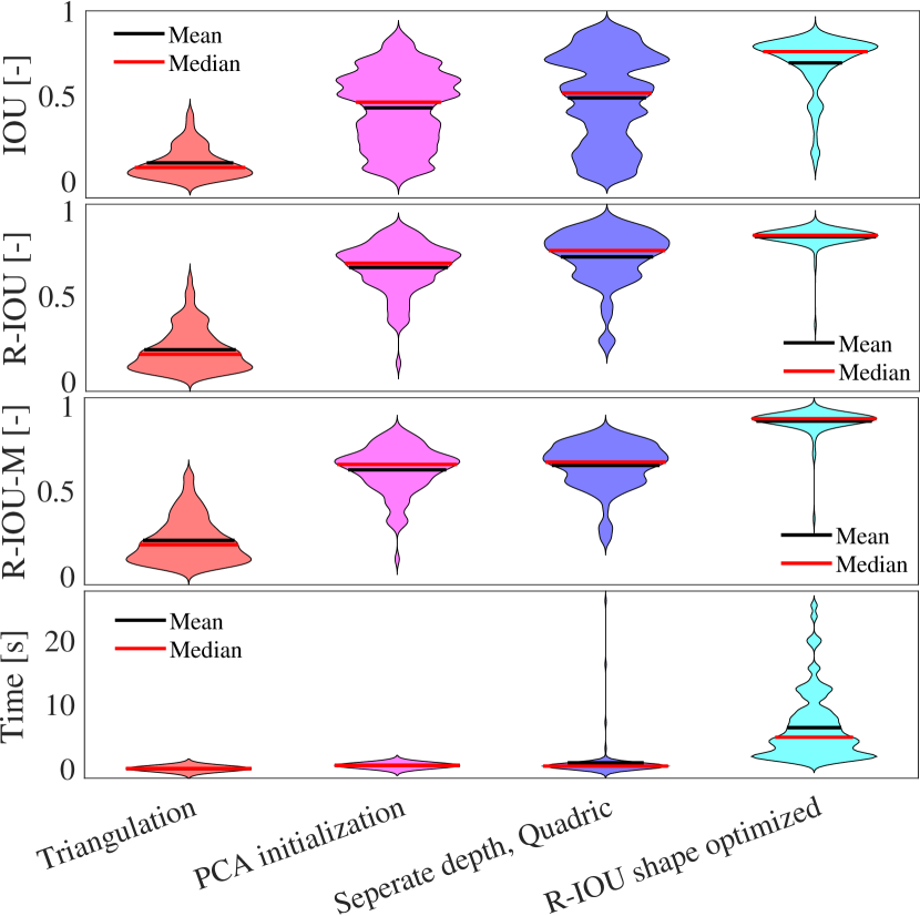
Figure 3: Result distribution of the evaluation metrics for 100 random SQs after different stages for the stage combination 1$\rightarrow\;$2$\rightarrow\;$3D$\rightarrow\;$3A. The wider the violins, the more samples fall in that region.

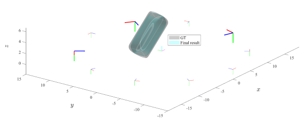
(a) Overview of the final result. The cameras whose observations are utilized in the optimization are highlighted with bold coordinate frames.

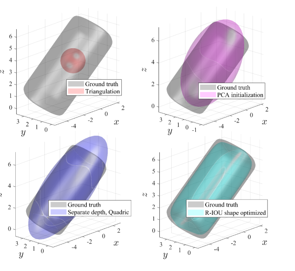
(b) Estimation and GT after different stages of the optimization.

Figure 4: Example SQ retrieval for the stage combination 1$\rightarrow\;$2$\rightarrow\;$3D$\rightarrow\;$3A.

V Conclusions and Outlook

In this work, we propose to use SQs to represent semantic objects for use in object-based semantic SLAM. We present numeric and analytic cost functions and introduce a multi-stage fitting procedure. With our novel approach, SQs are retrieved from multi-view semantic mask observations from a monocular camera exploring an environment. We show in preliminary experiments using various optimization setups in a simulation environment that SQ parameters are successfully recovered achieving high IOUs and R-IOUs.

However, the performance is not optimal, and the benefit SQs provide compared to standard quadrics is not always significant. Nevertheless, we see a lot of potential for robustness and accuracy improvement. The investigation of other non-linear optimization approaches, such as DIRECT [53] or StoGO [54], might improve the fragility with respect to local minima. However, as most optimization-based SLAM frameworks are based on Levenberg-Marquart optimization, the inclusion in such frameworks might become more challenging. Furthermore, the optimal cost function might not have been found yet and requires further investigation. Additional combinations and adaptions of the proposed cost functions and sampling procedures might lead to a faster convergence, increased robustness, and higher accuracy. Finally, the extension to real-world data and full optimization of SQ parameters together with camera poses, which would allow the inclusion in a SLAM framework, are subject to our current and future work.

Nevertheless, we believe that SQs are a promising representation of semantic objects in an environment enabling appearance-invariant loop-closures and localizations [33, 28] due to its compact and versatile parametrization. A semantically enriched map is easier to interpret for a human operator compared to traditional maps used in SLAM and provides improved situational awareness for high-level tasks such as motion planning or manipulation.

ADAS

advanced driving assistance systems

AE

auto-exposure

ASL

Autonomous Systems Lab

BA

bundle adjustment

BM

block-matching

BoW

Bag-of-Words

BRISK

Binary Rotation Invariant Scalable Keypoint

CLAHE

contrast limiting adaptive histogram equalization

CNN

Convolutional Neural Network

CPU

central processing unit

DAVIS

Dynamic and Active Vision Sensor

DCNN

Deep Convolutional Neural Network

DL

deep learning

DoF

degrees of freedom

DSO

Direct Sparse Odometry

DVS

Dynamic Vision Sensor

EKF

extended Kalman filter

ETCS

European Train Control System

ETSC

European Train Security Council

ESDF

Euclidean signed distance field

FAST

Features form Accelerated Segment Test

FC

fully connected

FIR

finite impulse response

FoV

field of view

FPGA

field-programmable gate array

FPS

frames per second

GNSS

global navigation satellite system

GP

Gaussian Process

GPM

Gaussian preintegrated measurement

GPS

Global Positioning System

GPU

graphics processing unit

GT

ground truth

GTC

ground truth clustering

GTSAM

Georgia Tech Smoothing and Mapping library

HDR

High Dynamic Range

HS

Hough space

HT

Hough transform

I²C

Inter-Integrated Circuit

IDOL

IMU-DVS Odometry with Lines

IMU

inertial measurement unit

INS

inertial navigation system

IOU

intersection over union

KF

Kalman filter

LED

light emitting diode

LiDAR

Light Detection and Ranging sensor

LSD

line segment detector

LSSVM

least squares support vector machine

LWIR

long-wave infrared

MAV

micro aerial vehicle

MCU

micro controller unit

NCLT

North Campus Long-Term

NMI

normalized mutual information

NMS

non-maxima suppression

NN

nearest neighbor

OS

operating system

PCB

printed circuit board

PC

point cloud

PCA

principal component analysis

PCM

probabilistic curvemap

PF

particle filter

PPS

Pulse per second

PTP

Precision Time Protocol

RANSAC

random sample consensus

RGB-D-I

Color-Depth-Inertial

R-IOU

reprojection intersection over union

RMSE

root mean square error

RNN

recurrent neural network

ROI

region of interest

ROS

Robot Operating System

RQE

Rényi’s Quadric Entropy

RTK

real time kinematics

SBB

Schweizerische Bundesbahnen

SIFT

Scale Invariant Feature Transform

SLAM

Simultaneous Localization And Mapping

SNN

spiking neural network

SNR

signal to noise ratio

SP

SuperPoint

SPI

Serial Peripheral Interface

SQ

superquadric

SWE

Sliding Window Estimator

ToF

time of flight

TSDF

Truncated Signed Distance Function

TUM

Technische Universität München

UART

Universal Asynchronous Receiver Transmitter

UAV

unmanned aerial vehicle

USB

universal serial bus

VBG

Verkehrsbetriebe Glattal AG

VBZ

Verkehrsbetriebe Zürich

VersaVIS

Open Versatile Multi-Camera Visual-Inertial Sensor Suite

VI

visual-inertial

VIO

visual-inertial odometry

VO

visual odometry

ZVV

Zürich Verkehrsverein

SVD

Singular Value Decomposition

DLT

Direct Linear Transform

UGV

unmanned ground vehicle

AR

augmented reality

VR

virtual reality

ATO

autonomous train operation

References

- [1] A. Gawel, R. Siegwart, M. Hutter, T. Sandy, H. Blum, J. Pankert, K. Kramer, L. Bartolomei, S. Ercan, F. Farshidian, M. Chli, and F. Gramazio, “A Fully-Integrated Sensing and Control System for High-Accuracy Mobile Robotic Building Construction,” in IEEE International Conference on Intelligent Robots and Systems. Institute of Electrical and Electronics Engineers Inc., 11 2019, pp. 2300–2307.
- [2] M. Blösch, S. Weiss, D. Scaramuzza, and R. Siegwart, “Vision based MAV navigation in unknown and unstructured environments,” in Proceedings - IEEE International Conference on Robotics and Automation, 2010, pp. 21–28.
- [3] M. Bürki, C. Cadena, I. Gilitschenski, R. Siegwart, and J. Nieto, “Appearance‐based landmark selection for visual localization,” Journal of Field Robotics, vol. 36, no. 6, pp. 1041–1073, 9 2019.
- [4] F. Tschopp, T. Schneider, A. W. Palmer, N. Nourani-Vatani, C. Cadena, R. Siegwart, and J. Nieto, “Experimental comparison of visual-aided odometry methods for rail vehicles,” IEEE Robotics and Automation Letters, vol. 4, no. 2, pp. 1815–1822, 2019.
- [5] R. Siegwart, I. R. Nourbakhsh, and D. Scaramuzza, Introduction to Autonomous Mobile Robots, 2nd ed. Camebridge: MIT Press, 2011.
- [6] T. Schneider, M. Dymczyk, M. Fehr, K. Egger, S. Lynen, I. Gilitschenski, and R. Siegwart, “maplab: An Open Framework for Research in Visual-inertial Mapping and Localization,” IEEE Robotics and Automation Letters, vol. 3, no. 3, pp. 1418–1425, 11 2018.
- [7] R. R. Mur-Artal, J. M. M. Montiel, and J. D. Tardos, “ORB-SLAM: A Versatile and Accurate Monocular SLAM System,” IEEE Transactions on Robotics, vol. 31, no. 5, pp. 1147–1163, 10 2015. [Online]. Available: http://ieeexplore.ieee.org/document/7219438/
- [8] S. Leutenegger, M. M. Chli, and R. Y. Siegwart, “Binary Robust Invariant Scalable Keypoints,” in Proceedings of the IEEE International Conference on Computer Vision, Barcelona, 2011, pp. 2548–2555. [Online]. Available: https://www.robots.ox.ac.uk/ vgg/rg/papers/brisk.pdf
- [9] E. Rublee, V. Rabaud, K. Konolige, and G. Bradski, “ORB: An efficient alternative to SIFT or SURF,” in Proceedings of the IEEE International Conference on Computer Vision, 2011, pp. 2564–2571.
- [10] M. J. Milford and G. F. Wyeth, “SeqSLAM: Visual route-based navigation for sunny summer days and stormy winter nights,” in 2012 IEEE International Conference on Robotics and Automation. IEEE, 5 2012, pp. 1643–1649. [Online]. Available: http://ieeexplore.ieee.org/document/6224623/
- [11] T. Sattler, W. Maddern, C. Toft, A. Torii, L. Hammarstrand, E. Stenborg, D. Safari, M. Okutomi, M. Pollefeys, J. Sivic, F. Kahl, and T. Pajdla, “Benchmarking 6DOF Outdoor Visual Localization in Changing Conditions,” in Proceedings of the IEEE Computer Society Conference on Computer Vision and Pattern Recognition. IEEE Computer Society, 12 2018, pp. 8601–8610.
- [12] R. Mur-Artal and J. D. Tardos, “ORB-SLAM2: An Open-Source SLAM System for Monocular, Stereo, and RGB-D Cameras,” IEEE Transactions on Robotics, pp. 1–8, 2017.
- [13] J. Engel, V. Koltun, and D. Cremers, “Direct Sparse Odometry,” IEEE Transactions on Pattern Analysis and Machine Intelligence, 2018.
- [14] K. He, G. Gkioxari, P. Dollar, and R. Girshick, “Mask R-CNN,” in Proceedings of the IEEE International Conference on Computer Vision, Singapore, 2017, pp. 2980–2988.
- [15] D. Bolya, C. Zhou, F. Xiao, and Y. J. Lee, “YOLACT++: Better Real-time Instance Segmentation,” IEEE Transactions on Pattern Analysis and Machine Intelligence, 2020.
- [16] J. Redmon, S. Divvala, R. Girshick, and A. Farhadi, “You only look once: Unified, real-time object detection,” in Proceedings of the IEEE Computer Society Conference on Computer Vision and Pattern Recognition, vol. 2016-Decem. IEEE Computer Society, 12 2016, pp. 779–788.
- [17] B. Verhagen, R. Timofte, and L. Van Gool, “Scale-invariant line descriptors for wide baseline matching,” in 2014 IEEE Winter Conference on Applications of Computer Vision, WACV 2014. IEEE Computer Society, 2014, pp. 493–500.
- [18] J. H. Lee, S. Lee, G. Zhang, J. Lim, W. K. Chung, and I. H. Suh, “Outdoor place recognition in urban environments using straight lines,” in Proceedings - IEEE International Conference on Robotics and Automation. Institute of Electrical and Electronics Engineers Inc., 9 2014, pp. 5550–5557.
- [19] B. Micusik and H. Wildenauer, “Descriptor free visual indoor localization with line segments,” in Proceedings of the IEEE Computer Society Conference on Computer Vision and Pattern Recognition, vol. 07-12-June-2015. IEEE Computer Society, 10 2015, pp. 3165–3173.
- [20] A. Oliva and A. Torralba, “Building the gist of a scene: the role ofal image features in recognition glob,” Progress in Brain Research, vol. 155 B, pp. 23–36, 2006. [Online]. Available: https://pubmed.ncbi.nlm.nih.gov/17027377/
- [21] R. Arandjelovic and A. Zisserman, “All about VLAD,” in Proceedings of the IEEE Computer Society Conference on Computer Vision and Pattern Recognition, Portland, OR, USA, 2013, pp. 1578–1585.
- [22] R. Arandjelovic, P. Gronat, A. Torii, T. Pajdla, and J. Sivic, “NetVLAD: CNN Architecture for Weakly Supervised Place Recognition,” IEEE Transactions on Pattern Analysis and Machine Intelligence, vol. 40, no. 6, pp. 1437–1451, 6 2018.
- [23] A. Gawel, C. Del Don, R. Siegwart, J. Nieto, and C. Cadena, “X-View: Graph-Based Semantic Multi-View Localization,” IEEE Robotics and Automation Letters, vol. 3, no. 3, pp. 1687–1694, 2017.
- [24] F. Taubner, F. Tschopp, T. Novkovic, R. Siegwart, and F. Furrer, “LCD - Line Clustering and Description for Place Recognition,” in Proceedings - 2020 International Conference on 3D Vision, 3DV 2020. Institute of Electrical and Electronics Engineers Inc., 11 2020, pp. 908–917.
- [25] J. L. Schönberger, M. Pollefeys, A. Geiger, and T. Sattler, “Semantic Visual Localization,” in 2018 IEEE/CVF Conference on Computer Vision and Pattern Recognition, Salt Lake City, UT, USA, 2017.
- [26] A. Cramariuc, F. Tschopp, N. Alatur, S. Benz, T. Falck, M. Brühlmeier, B. Hahn, J. Nieto, and R. Siegwart, “SemSegMap – 3D Segment-based Semantic Localization,” submitted for publication, 2021.
- [27] L. Nicholson, M. Milford, and N. Sunderhauf, “QuadricSLAM: Dual quadrics from object detections as landmarks in object-oriented SLAM,” IEEE Robotics and Automation Letters, vol. 4, no. 1, pp. 1–8, 2019.
- [28] K. M. Frey, T. J. Steiner, and J. P. How, “Efficient constellation-based map-merging for semantic SLAM,” in Proceedings - IEEE International Conference on Robotics and Automation, vol. 2019-May, Montreal, Canada, 2019, pp. 1302–1308.
- [29] H. Strasdat, J. M. M. Montiel, and A. J. Davison, “Real-time monocular SLAM: Why filter?” in Proceedings - IEEE International Conference on Robotics and Automation, 2010, pp. 2657–2664.
- [30] F. Tschopp, C. Von Einem, A. Cramariuc, D. Hug, A. W. Palmer, R. Siegwart, M. Chli, and J. Nieto, “Hough2Map-Iterative Event-Based Hough Transform for High-Speed Railway Mapping,” IEEE Robotics and Automation Letters, vol. 6, no. 2, pp. 2745–2752, 4 2021.
- [31] S. Yang and S. Scherer, “CubeSLAM: Monocular 3-D Object SLAM,” IEEE Transactions on Robotics, vol. 35, no. 4, pp. 925–938, 2019.
- [32] J. Papadakis, A. Willis, and J. Gantert, “RGBD-Sphere SLAM,” in SoutheastCon 2018. St. Petersburg, FL, USA: Institute of Electrical and Electronics Engineers Inc., 10 2018.
- [33] K. Ok, K. Liu, K. Frey, J. P. How, and N. Roy, “Robust Object-based SLAM for High-speed Autonomous Navigation,” in 2019 International Conference on Robotics and Automation (ICRA), Montreal, Canada, 5 2019, pp. 669–675.
- [34] J. Mccormac, R. Clark, M. Bloesch, A. J. Davison, and S. Leutenegger, “Fusion++: Volumetric Object-Level SLAM Reconstructed Object Inventory Live Frame View Object-centric Map,” in 2018 International Conference on 3D Vision (3DV), 2018, pp. 32–41.
- [35] M. Grinvald, F. Furrer, T. Novkovic, J. J. Chung, C. Cadena, R. Siegwart, and J. Nieto, “Volumetric instance-aware semantic mapping and 3D object discovery,” IEEE Robotics and Automation Letters, vol. 4, no. 3, pp. 3037–3044, 7 2019.
- [36] M. Strecke, J. Stückler, J. Stueckler, and J. Stückler, “EM-Fusion: Dynamic Object-Level SLAM with Probabilistic Data Association,” in Proceedings of the IEEE International Conference on Computer Vision. Seoul, Korea: Institute of Electrical and Electronics Engineers Inc., 10 2019, pp. 5865–5874. [Online]. Available: http://arxiv.org/abs/1904.11781
- [37] A. Rosinol, M. Abate, Y. Chang, and L. Carlone, “Kimera: An Open-Source Library for Real-Time Metric-Semantic Localization and Mapping,” in Proceedings - IEEE International Conference on Robotics and Automation. Institute of Electrical and Electronics Engineers Inc., 5 2020, pp. 1689–1696.
- [38] D. Gálvez-López, M. Salas, J. D. Tardós, and J. M. Montiel, “Real-time monocular object SLAM,” Robotics and Autonomous Systems, vol. 75, pp. 435–449, 2016.
- [39] R. F. Salas-Moreno, R. A. Newcombe, H. Strasdat, P. H. Kelly, and A. J. Davison, “SLAM++: Simultaneous localisation and mapping at the level of objects,” in Proceedings of the IEEE Computer Society Conference on Computer Vision and Pattern Recognition. Portland, OR, USA: IEEE, 2013, pp. 1352–1359.
- [40] A. H. Barr, “Superquadrics and Angle-Preserving Transformations,” IEEE Computer Graphics and Applications, vol. 1, no. 1, pp. 11–23, 1981.
- [41] T. E. Boult and A. D. Gross, “Recovery Of Superquadrics From 3-D Information,” in Intelligent Robots and Computer Vision VI, vol. 0848. SPIE, 2 1988, p. 358.
- [42] K. Wu and M. D. Levine, “Recovering Parametric Geons from Multiview Range Data,” in 1994 Proceedings of IEEE Conference on Computer Vision and Pattern Recognition, Seattle, WA, USA, 1994.
- [43] Y. Zhang, “Experimental comparison of superquadric fitting objective functions,” Pattern Recognition Letters, vol. 24, no. 14, pp. 2185–2193, 2003.
- [44] K. Duncan, S. Sarkar, R. Alqasemi, and R. Dubey, “Multi-scale superquadric fitting for efficient shape and pose recovery of unknown objects,” in Proceedings - IEEE International Conference on Robotics and Automation. Karlsruhe, Germany: IEEE, 2013, pp. 4238–4243.
- [45] A. Makhal, F. Thomas, and A. P. Gracia, “Grasping Unknown Objects in Clutter by Superquadric Representation,” in 2018 Second IEEE International Conference on Robotic Computing (IRC), Laguna Hills, CA, USA, 10 2018. [Online]. Available: http://arxiv.org/abs/1710.02121
- [46] N. Vaskevicius and A. Birk, “Revisiting Superquadric Fitting: A Numerically Stable Formulation,” IEEE Transactions on Pattern Analysis and Machine Intelligence, vol. 41, no. 1, pp. 220–233, 1 2019.
- [47] D. Paschalidou, A. O. Ulusoy, and A. Geiger, “Superquadrics Revisited: Learning 3D Shape Parsing beyond Cuboids,” in Proceedings IEEE Conf. on Computer Vision and Pattern Recognition (CVPR), Long Beach, USA, 4 2019. [Online]. Available: http://arxiv.org/abs/1904.09970
- [48] A. Jaklič, A. Leonardis, and F. Solina, “Superquadrics and Their Geometric Properties,” in Segmentation and Recovery of Superquadrics, Computational Imaging and Vision. Dordrecht: Springer, 2000, vol. 20, pp. 13–39.
- [49] K. Levenberg, “A method for the solution of certain non-linear problems in least squares,” Quarterly of Applied Mathematics, vol. 2, no. 2, pp. 164–168, 7 1944. [Online]. Available: https://www.ams.org/qam/1944-02-02/S0033-569X-1944-10666-0/
- [50] D. W. Marquardt, “An Algorithm for Least-Squares Estimation of Nonlinear Parameters,” Journal of the Society for Industrial and Applied Mathematics, vol. 11, no. 2, pp. 431–441, 6 1963.
- [51] MathWorks Schweiz, “polyshape - 2-D polygons in MATLAB,” 2017. [Online]. Available: https://ch.mathworks.com/help/matlab/ref/polyshape.html
- [52] J. Shlens, “A Tutorial on Principal Component Analysis,” Google Research, Mountain View, CA 94043, Tech. Rep., 4 2014.
- [53] D. R. Jones, C. D. Perttunen, and B. E. Stuckman, “Lipschitzian optimization without the Lipschitz constant,” Journal of Optimization Theory and Applications, vol. 79, no. 1, pp. 157–181, 10 1993. [Online]. Available: https://link.springer.com/article/10.1007/BF00941892
- [54] K. Madsen and S. Zertchaninov, “Global Optimization using Branch-and-Bound,” Department of Mathematical Modelling, Technical University of Denmark, Tech. Rep., 1998.