Efficient Representations of Signals in
Nonlinear Signal Processing
with Applications to Inverse Problems

Abstract

The focus of this thesis is the construction and analysis of efficient representations in nonlinear signal processing, and the applications of these structures to inverse problems in a variety of fields. The work is composed of three major sections, each associated with a different form of data:

• Regression and Distance Estimation on Graphs and Riemannian Manifolds.

• Instantaneous Time-Frequency Analysis via Synchrosqueezing.

• Multiscale Dictionaries of Slepian Functions on the Sphere.

September 2011 Peter J. Ramadge and Ingrid Daubechies Electrical Engineering

Chapter 1 Introduction

This chapter introduces the main topics covered in this thesis, and the major tools and ideas that link these topics. The discussion is philosophical and purely motivational, and should not be considered mathematically rigorous or exhaustive. Chapters 2, 3, 5, and 7 contain their own relevant introductory discussions, descriptions of prior work, and literature reviews.

An inverse problem is a general question of the following form:

You are given observed measurements $Y=F(X)$, where $F:D\to R$, is a mapping from domain $D$ to range $R$. Provide an estimate of a physical object or underlying set of parameters $X$.

Inverse problems encompass a variety of types of questions in many fields, from geophysics and medical imaging to computer graphics. In a high level sense, all of the following questions are inverse problems:

• Given the output of a CT scanner (sinogram), reconstruct the 3D volumetric image of the patient’s chest.

• Given noisy and limited satellite observations of the magnetic field over Australia, estimate the magnetic field everywhere on the continent.

• Given the lightcurve of a periodic dwarf star, extract the significant slowly time-varying modes of oscillation. Determine which modes are associated with the rotation of the star, which are caused by transiting giant planets, and which are caused by one or more earth-sized planets.

• Given a spline curve corrupted by additive Gaussian noise, identify its order, knot positions, and the parameters at each knot.

• Given a social network graph with a variety of both known and unknown parameters at each node, and given a sample of known zip codes on a subset of the graph, estimate the zip codes of the rest of the nodes.

Of the questions above, only the first two are traditionally considered to be inverse problems because they have a clear physical system $F(\cdot)$ mapping inputs to outputs, and the domain and range are also clear from the physics of the problem. Nevertheless, all of these problems can be formulated as general inverse problems: a domain and range are given, as are observations, and the simplest, most accurate, or most statistically likely parameters to match the observations are required. This basic premise encourages the “borrowing” and mixing of ideas from many fields of mathematics and engineering: graph theory, statistics, functional analysis, differential equations, and geometry.

This thesis focuses on finding representations of the data $X$, or of the underlying transform $F(\cdot)$, that lead to either simpler or more robust ways to solve particular inverse problems, or that provide a new perspective for existing solutions.

We especially focus on finding representations within domains $D$ which are important in fields such as medical imaging and geoscience, or are becoming important in the signal processing community due to the recent explosion of “high dimensional” data sets. These domains are:

• General compact Riemannian manifolds.

• Large graphs (especially nearest neighbor graphs from point samples of Riemannian manifolds embedded in ${\mathbb{R}}^{p}$).

• The Sphere $S^{2}$.

A short technical description of Riemannian manifolds, and a set of references, is given in App. A. A description of (Nearest Neighbor) graphs can be found in §2.2.

The central tool that brings together all of the problems, constructions, and insights in our work is the Laplacian. In a way, the thrust of this thesis is the importance and flexibility of the Laplacian as a data analysis and problem solving tool. Roughly speaking, the Laplacian is defined as follows:

Given a domain $D$, with measure $\mu$ and knowing for any point $x\in D$ its neighborhood $N(x)$, the Laplacian $L$ is a linear operator that, for any well defined function $f(x)$, subtracts some weighted average of $f(\cdot)$ in $N(x)$ from its value at $x$: $$[Lf](x)=f(x)-\int_{x^{\prime}\in N(x)}w(x,x^{\prime})f(x^{\prime})d\mu(x^{\prime}),$$ where the weights are determined by the intrinsic relationship (e.g., distance) between $x$ and $x^{\prime}$ on $D$.

The Laplacian is a powerful tool because it synthesizes local information at each point $x$ in domain $D$ into global information about the domain; and this in turn can be used to analyze functions and other operators on this domain. This statement is formalized in the classical language of Fourier analysis and the recent work of Mikhail Belkin, Ronald Coifman, Peter Jones, and Amit Singer [5, 23, 53, 97]: the eigenfunctions of the Laplacian are a powerful tool for both the analysis of points in $D$ and functions defined on $D$.

Throughout this thesis, we use and study a variety of Laplacians, each for a slightly different purpose:

• The weighted graph Laplacian: its “averaging” component in Chapter 2 and its regularized inverse in Chapters 3 and 4.

• The Laplace-Beltrami on a compact Riemannian manifold in Chapters 3 and 4.

• The Fourier transform (projections on the eigenfunctions of the Laplacian on ${\mathbb{R}}$) in Chapters 5 and 6.

• Spherical harmonics (eigenfunctions of the Laplace-Beltrami operator on $S^{2}$) and their use in analyzing bandlimited functions on the sphere in Chapter 7.

The definition and properties of the weighted graph Laplacian are given in §3.3.3. A definition of the Laplacian for a compact Riemannian manifold is given in App. A, with specific definitions for the real line and the sphere in App. B. This appendix also contains a comprehensive discussion of Fourier analysis on Riemannian manifolds, and on the Sphere in particular.

Though the definition of the Laplacian differs depending on the underlying domain $D$, all Laplacians are intricately linked: the Laplacian on a domain $D$ converges to that on $D^{\prime}$ as the former domain converges to the latter, or when one is a special case of the other. We study these relationships when they are relevant (e.g., in §3.3.3).

The term Nonlinear in the title of this thesis refers to the ways in which our constructions use properties of the Laplacian, or of its eigenfunctions, to represent data:

• In Chapter 2, the regularized inverse of the graph Laplacian is used to denoise graphs (this is not directly clear from the context but see §4.6 for a discussion).

• In Chapters 3 and 4, the regularized inverse of both the graph Laplacian, and the Laplace Beltrami operator, are analyzed; and a special “trick” of taking the nonlinear logarithm is used to both perform regression and to estimate geodesic distances.

• In Chapters 5 and 6, the Fourier transform of the Wavelet representation of harmonic signals is used to motivate a time localized estimate of amplitude and frequency. This is followed up by a nonlinear reassignment of the Wavelet representation.

• In Chapter 7, we construct a multi-scale dictionary composed of bandlimited Slepian functions on the sphere (which are in turn constructed via Fourier analysis). This dictionary is then combined with nonlinear ($\ell_{1}$) methods for signal estimation.

We hope that the underlying theme of this thesis is now clear: as the movie Manhattan is Woody Allen’s ode to the city of New York, the work herein is a testament to the flexibility and power of the Laplacian.

Without further ado, we now describe in detail the focus of the individual chapters of this thesis.

1.1 Denoising and Inference on Graphs

Many unsupervised and semi-supervised learning problems contain relationships between sample points that can be modeled with a graph. As a result, the weighted adjacency matrix of a graph, and the associated graph Laplacian, are often used to solve such problems. More specifically, the spectrum of the graph Laplacian, and its regularized inverse, can both be used to determine relationships between observed data points (such as “neighborliness” or “connectedness”), and to perform regression when a partial labeling of the data points is available. Chapters 2, 3, and 4 study the inverse regularized graph Laplacian.

Chapter 2 focuses on the unsupervised problem of detecting “bad” edges, or bridges, in a graph constructed with erroneous edges. Such graphs arise, e.g., as nearest neighbor graphs from high dimensional points sampled under noise. A novel bridge detection rule is constructed, based on Markov random walks with restarts, that robustly identifies bridges. The detection rule uses the regularized inverse of the graph’s Laplacian matrix, and its structure can be analyzed from a geometric point of view under certain assumptions of the underlying sample points. We compare this detection rule to past work and show its improved performance as a preprocessing step in the estimation of geodesic distances on the underlying graph, a global estimation problem. We also show its superior performance as a preprocessing tool when solving the random projection computational tomography inverse problem.

Chapter 3 studies a closely related problem, that of performing regression on points sampled from a high dimensional space, only some of which are labeled. We focus on the common case when the regression is performed via the nearest neighbor graph of the points, with ridge and Laplacian regularization. This common solution approach reduces to a matrix-vector product, where the matrix is the regularized inverse of the graph Laplacian, and the vector contains the partially known label information.

In this chapter, we focus on the geometric aspects of the problem. First, we prove that in the noiseless, low regularization case, when the points are sampled from a smooth, compact, Riemannian manifold, the matrix-vector product converges to a sampling of the solution to a elliptic PDE. We use the theory of viscosity solutions to show that in the low regularization case, the solution of this PDE encodes geodesic distances between labeled points and unlabeled ones. This geometric PDE framework provides key insights into the original semisupervised regression problem, and into the regularized inverse of the graph Laplacian matrix in general.

Chapter 4 follows on the theoretical analysis in Chapter 3 by displaying a wide variety of applications for the Regularized Laplacian PDE framework. The contributions of this chapter include:

• A new consistent geodesics distance estimator on Riemannian manifolds, whose complexity depends only on the number of sample points $n$, rather than the ambient dimension $p$ or the manifold dimension $d$.

• A new multi-class classifier, applicable to high-dimensional semi-supervised learning problems.

• New explanations for negative results in the machine learning literature associated with the graph Laplacian.

• A new dimensionality reduction algorithm called Viscous ISOMAP.

• A new and satisfying interpretation for the bridge detection algorithm constructed in Chapter 2.

1.2 Instantaneous Time-Frequency Analysis

Time frequency analysis in the form of the Fourier transform, short time Fourier transform (STFT), and their discrete variants (e.g. the power spectrum), have long been standard tools in science, engineering, and mathematical analysis. Recent advances in time-frequency reassignment, wherein energies in the magnitude plot of the STFT are shifted in the time-frequency plane, have found application in “sharpening” images of, e.g., STFT magnitude plots, and have been used to perform ridge detection and other types of time- and frequency-localized feature detection in time series.

Chapters 5 and 6 focus on a novel time-frequency reassignment transform, Synchrosqueezing, which can be constructed to work “on top of” many invertible transforms (e.g., the Wavelet transform or the STFT). As Synchrosqueezing is itself an invertible transform, it can be used to filter and denoise signals. Most importantly, it can be used to extract individual components from superpositions of “quasi-harmonic” functions: functions that take the form $A(t)e^{i\phi(t)}$, where $A(t)$ and $d\phi(t)/dt$ are slowly varying.

Chapter 5 focuses on two aspects of Synchrosqueezing. First, we develop a fast new numerical implementation of Wavelet-based Synchrosqueezing. This implementation, and other useful utilities, have been included in the Synchrosqueezing MATLAB toolbox. Second, we present a stability theorem, showing that Synchrosqueezing can extract components from superpositions of quasi-harmonic signals when the original observations have been corrupted by bounded perturbations (of the form often encountered during the pre-processing of signals).

Chapter 6 builds upon the work of the previous chapter to develop novel applications of Synchrosqueezing. We present a wide variety of problem domains in which the Synchrosqueezing transform is a powerful tool for denoising, feature extraction, and more general scientific analysis. We especially focus on estimation in inverse problems in medical signal processing and the geosciences. Contributions include:

• The extraction of respiratory signals from ECG (Electrocardiogram) signals.

• Precise new analyses of paleoclimate simulations (solar insolation models), individual paleoclimate proxies, and proxy stacks in the last 2.5 Myr. These results are compared to Wavelet- and STFT-based analyses, which are less precise and harder to interpret.

1.3 Multiscale Dictionaries of Slepian Functions on the Sphere

Just as audio signals and images are constrained by the physical processes that generate them, and by the sensors that observe them, so too are many geophysical and cosmological signals, which reside on the sphere $S^{2}$. On the real line and in the plane, both physical constraints and sampling constraints lead to assumptions of a bandlimit: that a signal contains zero energy outside some supporting region in the frequency domain. Similarly, bandlimited signals on the sphere are zero outside the low-frequency spherical harmonic components.

In Chapter 7, following up on Claude Shannon’s initial investigations into sampling, we describe Slepian, Landau, and Pollak’s spatial concentration problem on subsets of the real line, and the resulting Slepian functions. The construction of Slepian functions have led to many important modern algorithms for the inversion of bandlimited signals from their samples within an interval, and especially Thompson’s multitaper spectral estimator. We then study Simons and Dahlen’s extension of these results to subsets of the Sphere, where now the definition of frequency and bandlimit has been appropriately modified.

Building upon these results, we develop an algorithm for the construction of dictionary elements that are bandlimited, multiscale, and localized. Our algorithm is based on a subdivision scheme that constructs a binary tree from subdivisions of the region of interest (ROI). We show, via numerous examples, that this dictionary has many nice properties: it closely overlaps with the most concentrated Slepian functions on the ROI, and most element pairs have low coherence.

The focus of this construction is to solve ill-posed inverse problems in geophysics and cosmology. Though the new dictionary is no longer composed of purely orthogonal elements like the Slepian basis, it can be combined with modern inversion techniques that promote sparsity in the solution, to provide significantly lower residual error after reconstruction (as compared to classically optimal Slepian inversion techniques).

We provide additional numerical results showing the solution path that these techniques take when combined with the multiscale dictionaries, and their efficacy on a standard model of the Earth’s magnetic field, POMME-4. Finally, we show via randomized trials that the combination of the multiscale construction and $\ell_{1}$-based estimation provides significant improvement, over the current state of the art, in the inversion of bandlimited white and pink random processes within subsets of the sphere.

Chapter 2 Graph Bridge Detection via Random Walks

2.1 Introduction

Many new problems in machine learning and signal processing require the robust estimation of geodesic distances between nodes of a nearest neighbors (NN) graph. For example, when the nodes represent points sampled from a manifold, estimating feature space distances between these points can be an important step in unsupervised [105] and semi-supervised [6] learning. This problem often reduces to that of having accurate estimates of each point’s neighbors, as described below.

In the simplest approach to estimating geodesic distances, the NN graph’s edges are estimated from either the $k$ nearest neighbors around each point, or from all of the neighbors within an ambient (Euclidean) $\delta$-ball around each point. Each graph edge is then assigned a weight: the ambient distance between its nodes. A graph shortest path (SP) algorithm, e.g. Dijkstra’s [25, §24.3], is then used to estimate geodesic distances between pairs of points.

When the manifold is sampled with noise, or contains outliers, bridges (short circuits between distant parts of the manifold) can appear in the NN graph and this has a catastrophic effect on geodesics estimation [3].

In this chapter, we develop a new approach for calculating point “neighborliness” from the NN graph. This approach allows the robust removal of bridges from NN graphs of manifolds sampled with noise. This metric, which we call “neighbor probability,” is based on a Markov Random walk with independent restarts. The bridge decision rule based on this metric is called the neighbor probability decision rule (NPDR), and reduces to removing edges from the NN graph whose neighbor probability is below a threshold. We study some of the NPDR’s geometric properties when the number of samples grow large. We also compare the efficacy of the NPDR to other decision rules and show its superior performance on removing bridges in simulated data, and in the novel inverse problem of computational tomography with random (and unknown) projection angles.

2.2 Preliminaries

Let ${\mathcal{X}}=\left\{x_{i}\right\}_{i=1}^{n}$ be nonuniformly sampled points from manifold ${\mathcal{M}}\subset{\mathbb{R}}^{r}$. We observe ${\mathcal{Y}}=\left\{y_{i}=x_{i}+\nu_{i}\right\}_{i=1}^{n}$, where $\nu_{i}$ is noise. A nearest neighbor (NN) graph $G=({\mathcal{Y}},{\mathcal{E}},d)$ is constructed from $k$-NN or $\delta$-ball neighborhoods of ${\mathcal{Y}}$ with the scale ($k$ or $\delta$) chosen via cross-validation or prior knowledge. The map $d\colon{\mathcal{E}}\to{\mathbb{R}}$ assigns cost $d_{e}=\left\lVert x_{k}-x_{l}\right\rVert_{2}$ to edge $e=(k,l)\in{\mathcal{E}}$. Let ${\mathcal{D}}=\left\{d_{e}:e\in{\mathcal{E}}\right\}$. The set ${\mathcal{E}}$ gives initial estimates of neighbors on the manifold. Let ${\mathcal{F}}_{k}$ denote the neighbors of $x_{k}$ in $G$.

In [105] the geodesic distance between $(i,j)\in{\mathcal{Y}}^{2}$ is estimated by $\hat{g}_{ij}=\sum_{e\in{\mathcal{P}}_{ij}}d_{e}$ where ${\mathcal{P}}_{ij}$ is a minimum cost path from $i$ to $j$ in $G$ (this can be calculated via Dijkstra’s algorithm). When there is no noise, this estimate converges to the true geodesic distance on ${\mathcal{M}}$ as $n\to\infty$ and neighborhood size $\delta\to 0$. However, in the presence of noise bridges form in the NN graph and this results in significant estimation error. Forming the shortest path in $G$ is too greedy in the presence of bridges.

If bridges could be detected, their anomalous effect could be removed without disconnecting the graph by substituting a surrogate weight: ${\tilde{d}}_{e}=d_{e}+M,e\in{\mathcal{B}}$ where ${\mathcal{B}}$ is the set of detected bridges and $M=n(\max_{e\in{\mathcal{E}}}d_{e})$, larger than the diameter of $G$, is a penalty. Let ${\widetilde{G}}=({\mathcal{Y}},{\mathcal{E}},{\tilde{d}})$ and ${\widetilde{{\mathcal{P}}}}_{ij}$ be a minimum cost path between $i$ and $j$ in ${\widetilde{G}}$. The adjusted estimate of geodesic distance is ${\tilde{g}}_{ij}=\sum_{e\in{\widetilde{{\mathcal{P}}}}_{ij}}d_{e}$.

With this in mind, we first review some bridge detection methods, and discuss recent theoretical work in random walks on graphs.

2.3 Prior Work

The greedy nature of the SP solution encourages the traversal of bridges, thereby significantly underestimating geodesic distances. Previous work has considered denoising the nearest neighbors graph via rejection of edges based on local distance statistics [21, 96], or via local tangent space estimation [63, 18]. However, unlike the method we propose (NPDR), these methods use local rather that global statistics. We have found that using only local statistics can be unreliable. For example, with state of the art robust estimators of the local tangent space (as in [103]), local rejection of neighborhood edges is not reliable with moderate noise or outliers. Furthermore, edge removal (pruning) based on local edge length statistics is based on questionable assumptions. For example, a thin chain of outliers can form a bridge without unusually long edge lengths.

As an example, we first describe the simplest class of bridge decision rules (DRs): ones that classify bridges by a threshold on edge length. We call this the length decision rule (LDR); it is similar to the DR of [21]. It is calculated with the following steps:

1. Normalize edge lengths for local sampling density by setting

   $${\bar{d}}_{kl}=\frac{d_{kl}}{\sqrt{d_{k\cdot}d_{l\cdot}}},$$

   where $d_{k\cdot}=\sum_{m\in{\mathcal{F}}_{k}}d_{km}$ sums outgoing edge lengths from $x_{k}$.

2. Let ${\bar{{\mathcal{D}}}}=\left\{{\bar{d}}_{e}:e\in{\mathcal{E}}\right\}$. Select a “good edge percentage” $0<q<1$ (e.g. $99\%$) and calculate the detected bridge set ${\mathcal{B}}$ via:

   $${\mathcal{B}}=\left\{e\in{\mathcal{E}}\colon{\bar{d}}_{e}\geq Q({\bar{{\mathcal{D}}}},q)\right\},$$

   where $Q({\mathcal{D}},q)$ is the $q$-th quantile of the set ${\mathcal{D}}$.

The second decision rule, Jaccard similarity DR (JDR), classifies bridges as edges between points with dissimilar neighborhoods [96]. As opposed to the LDR, the JDR uses information from immediate neighbors of two points to detect bridges:

1. The Jaccard similarity between the neighborhoods of $x_{l}$ and $x_{m}$ is

   $$j_{lm}=\frac{\left\lvert{\mathcal{F}}_{l}\cap{\mathcal{F}}_{m}\right\rvert}{\left\lvert{\mathcal{F}}_{l}\cup{\mathcal{F}}_{m}\right\rvert}.$$

2. Let ${\mathcal{J}}=\left\{j_{e}:e\in{\mathcal{E}}\right\}$ be the set of Jaccard similarities. Select a $q\in(0,1)$; the estimated bridge set is

   $${\mathcal{B}}=\left\{e\in{\mathcal{E}}\colon j_{e}<Q({\mathcal{J}},1-q)\right\}.$$

We now describe a more global neighborliness metric. The main motivation is that bridges are short cuts for shortest paths. This suggests detecting bridges by counting the traversals of each edge by estimated geodesics. This is the concept of edge centrality (edge betweenness) in networks [76]. In a network, the centrality of edge $e$ is

$$BE(e)=\sum_{(i,j)\in{\mathcal{Y}}^{2}}{\mathbb{I}}(e\in{\mathcal{P}}_{ij}).$$

Edge centrality can be calculated in $O(n^{2}\log n)$ time and $O(n+\left\lvert{\mathcal{E}}\right\rvert)$ space using algorithms of Newman or Brandes [76, 11]. However, caution is required in using edge centrality for our purpose. Consider a bridge $(a,b)\in{\mathcal{E}}$ having high centrality. Suppose there exists a point $y_{c}$ with $(a,c),(c,b)\in{\mathcal{E}}$ such that $d_{ac}+d_{cb}<d_{ab}+\delta^{\prime}$, $\delta^{\prime}$ small. These edges are never preferred over $(a,b)$ in a geodesic path, hence have low centrality. However, once $(a,b)$ is placed into ${\mathcal{B}}$ and given increased weight, $(a,c),(c,b)$ reveals itself as a secondary bridge in ${\widetilde{G}}$. So detection by centrality must be done in rounds, each adding edges to ${\mathcal{B}}$. This allows secondary bridges to be detected in subsequent rounds. We now describe the Edge Centrality Decision Rule (ECDR):

Select quantile $q\in(0,1)$ and iterate the following steps $K$ times on ${\widetilde{G}}$:

1. Calculate $BE(e)$ for each edge $e$.

2. Place $(1-q)n/K$ of the most central edges into ${\mathcal{B}}$ and update ${\widetilde{G}}$.

The result is a bridge set ${\mathcal{B}}$ containing approximately $\lfloor(1-q)n\rfloor$ edges, matching the $q$-th quantile sets of the previous DRs. The iteration count parameter $K$ trades off between computational complexity (higher $K$ implies more iterations of edge centrality estimation) and robustness (it also more likely to detect bridges). To our knowledge, the use of centrality as a bridge detector is new. While an improvement over LDR, the deterministic greedy underpinnings of ECDR are a limitation: it initially fails to see secondary bridges, and may also misclassify true high centrality edges as bridges, e.g. the narrow path in the dumbbell manifold [24].

The Diffusion Maps approach to estimating feature space distances [24], has experimentally exhibited robustness to noise, outliers, and finite sampling. Diffusion distances, based on random walks on the NN graph, are closely related to “natural” distances (commute times) on a manifold [45]. Furthermore, Diffusion Maps coordinates (based on these distances) converge to eigenfunctions of the Laplace Beltrami operator on the underlying manifold.

The neighbor probability metric we construct is a global measure of edge reliability based on diffusion distances. The NPDR, based on this metric, is then used to inform geodesic estimates.

2.4 Neighbor Probability Decision Rule

We now propose a DR based on a Markov random walk that assigns a probability that two points are neighbors. This steps back from immediately looking for a shortest path and instead lets a random walk “explore” the NN graph. To this end, let $P$ be a row-stochastic matrix with $P_{ij}=0$ if $i\neq j$ and $(i,j)\notin{\mathcal{E}}$. Let $p\in(0,1)$ be a parameter and ${\bar{p}}=1-p$. Consider a random walk $s(m)$, $m=0,1,\ldots$, on $G$ starting at $s(0)=i$ and governed by $P$. For each $t\geq 0$, with probability $p$ we stop the walk and declare $s(m)$ a neighbor of $i$. Let $N$ be the matrix of probabilities that the walk starting at node $i$, stops at node $j$. The $i$-th row of $N$ is the neighbor distribution of node $i$. This distribution can be calculated:

$$N_{ij} =\sum_{m=0}^{\infty}\Pr(\text{stop at $m$},y^{(m)}=y_{j}|y^{(0)}=y_{i})$$ (2.1)

$$=\sum_{m=0}^{\infty}\Pr(\text{stop at $m$})\Pr(y^{(m)}=y_{j}|y^{(0)}=y_{i})$$ (2.2)

$$=\sum_{m=0}^{\infty}\Pr(\text{stop at $m$})\left(P^{m}\right)_{ij}$$ (2.3)

$$=\sum_{m=0}^{\infty}p(1-p)^{m}\left(P^{m}\right)_{ij}.$$ (2.4)

In (2.1) we decompose the stopping event into the disjoint events of stopping at time $t$. In (2.2) we separate the independent events of stopping from being at the current position $y^{(m)}$. In (2.3) we use the well known Markov property $P_{ij}^{(m)}=\left(P^{m}\right)_{ij}$ (with $P^{(0)}=I$). Finally, in (2.4) we recall that stopping at time $m$ means we choose not to stop, independently, for each $m^{\prime}=0,\ldots,m-1$, and finally stop at time $m$, so the probability of this event is $(1-p)^{m}p$. Thus, the neighbor probabilities are:

$$N=\sum_{t\geq 0}p(1-p)^{m}P^{m}=p(I-{\bar{p}}P)^{-1}.$$

A smaller stopping probability $p$ induces greater weighting of long-time diffusion effects, which are more dependent on the topology of ${\mathcal{M}}$. $N$ is closely related to the normalized commute time of [114]. Its computation requires $O(n^{3})$ time and $O(n^{2})$ space ($P$ is sparse but $N$ may not be).

The neighborhood probability matrix $N$ is heavily dependent on the choice of underlying random walk matrix $P$. First we relate several key properties of $N$ to those of $P$, then we introduce a geometrically intuitive choice of $P$ when the sample points are sampled from a manifold.

Lemma 2.4.1.

$N$ is row-stochastic, shares the left and right eigenvectors of $P$, and has spectrum $\sigma(N)=\{p(1-{\bar{p}}\lambda)^{-1}$, $\lambda\in\sigma(P)\}$.

Proof.

Clearly, $N^{-1}=(I-{\bar{p}}P)/p$ is row-stochastic, shares the left and right eigenvectors of $P$ and has spectrum $\{(1-{\bar{p}}\lambda)/p,\lambda\in\sigma(P)\}$. ∎

Following [24], we select $P$ to be the popular Diffusion Maps kernel on $G$:

1. Choose $\epsilon>0$ (e.g. $\epsilon=\operatorname*{med}_{e\in{\mathcal{E}}}d_{e}/2$) and let $({\hat{P}_{\epsilon}})_{lk}=\exp\left(-d_{kl}^{2}/\epsilon\right)$ if $(l,k)\in{\mathcal{E}}$, $1$ if $l=k$, and $0$ otherwise.

2. Let ${\hat{D}_{\epsilon}}$ be diagonal with $({\hat{D}_{\epsilon}})_{kk}=\sum_{l}({\hat{P}_{\epsilon}})_{kl}$, and normalize for sampling density by setting ${A_{\epsilon}}={\hat{D}_{\epsilon}}^{-1}{\hat{P}_{\epsilon}}{\hat{D}_{\epsilon}}^{-1}$.

3. Let ${D_{\epsilon}}$ be diagonal with $({D_{\epsilon}})_{kk}=\sum_{l}({A_{\epsilon}})_{kl}$ and set ${P_{\epsilon}}={D_{\epsilon}}^{-1}{A_{\epsilon}}$.

${P_{\epsilon}}$ is row-stochastic and, as is well known, has bounded spectrum:

Lemma 2.4.2.

The spectrum of ${P_{\epsilon}}$ is contained in $[0,1]$.

Proof.

${\hat{P}_{\epsilon}}$, ${A_{\epsilon}}$ and $S={D_{\epsilon}}^{-1/2}{A_{\epsilon}}{D_{\epsilon}}^{-1/2}$, are symmetric PSD. ${P_{\epsilon}}={D_{\epsilon}}^{-1}{A_{\epsilon}}$ is row-stochastic and similar to $S$. ∎

We define the Neighbor Probability Decision Rule (NPDR) as follows.

1. Let ${N_{\epsilon}}=p(I-{\bar{p}}{P_{\epsilon}})^{-1}$ and find the restriction ${\mathcal{N}}=\left\{({N_{\epsilon}})_{e}:e\in{\mathcal{E}}\right\}$ of ${N_{\epsilon}}$ to ${\mathcal{E}}$.

2. Choose a $q\in(0,1)$ and let ${\mathcal{B}}=\left\{e\in{\mathcal{E}}:({N_{\epsilon}})_{e}<Q({\mathcal{N}},1-q)\right\}$, i.e., edges connecting nodes with a low probability of being neighbors, are bridges.

Calculating ${N_{\epsilon}}$ can be prohibitive for very large datasets. Fortunately, we can effectively order the elements of ${\mathcal{N}}$ using a low rank approximation to ${N_{\epsilon}}$.

By Lemmas 2.4.1, 2.4.2, we calculate $N_{lm}\approx\sum_{j=1}^{J}p(1-{\bar{p}}\lambda_{j})^{-1}(v^{R}_{j})_{l}(v^{L}_{j})_{m}$ for $(l,m)\in{\mathcal{E}}$, where $\lambda_{j}$,$v^{R}_{j}$ and $v^{L}_{j}$ are the $J$ largest eigenvalues of ${P_{\epsilon}}$ and the associated right and left eigenvectors. In practice, an effective ordering of ${\mathcal{N}}$ is obtained with $J\ll n$ and since ${P_{\epsilon}}$ is sparse, its largest eigenvalues and eigenvectors can be computed efficiently using a standard iterative algorithm.

Matrix ${N_{\epsilon}}$ has, thanks to our choice of ${P_{\epsilon}}$, a more geometric interpretation which we now discuss.

2.4.1 Geometric Interpretation of $N$

In this section, we show the close relationship between the matrices ${N_{\epsilon}}$, ${P_{\epsilon}}$, and the weighted graph Laplacian matrix (to be defined soon). One important property of ${P_{\epsilon}}$ is its relationship to the Laplace Beltrami operator on ${\mathcal{M}}$. Specifically, when $n\to\infty$, and as $\epsilon\to 0$ at the appropriate rate , $(I-{P_{\epsilon}})/\epsilon\to c\Delta_{LB}$ both pointwise and in spectrum [24]. Here ${L_{\epsilon}}=(I-{P_{\epsilon}})/\epsilon$ is the weighted graph Laplacian and $\Delta_{LB}$ is the Laplace Beltrami operator on ${\mathcal{M}}$ and $c$ is a constant. Thus, for large $n$ and small $\epsilon$, ${P_{\epsilon}}$ is a neighborhood averaging operator. This property also holds for ${N_{\epsilon}}$:

Theorem 2.4.3.

As $n\to\infty$ and $\epsilon\to 0$, $(I-{N_{\epsilon}})/\epsilon\to c^{\prime}\Delta_{LB}$.

Proof.

For $I-S$ invertible, $(I-S)^{-1}=I+S(I-S)^{-1}$. From Lem. 2.4.2, $I-{\bar{p}}{P_{\epsilon}}$ is invertible. Thus

$$p(I-{\bar{p}}{P_{\epsilon}})^{-1} =\left(I-\frac{{\bar{p}}}{p}({P_{\epsilon}}-I)\right)^{-1}$$ (2.5)

$$=I+\frac{{\bar{p}}}{p}({P_{\epsilon}}-I)\left(I-\frac{{\bar{p}}}{p}({P_{\epsilon}}-I)\right)^{-1}.$$ (2.6)

Therefore

$$\frac{I-{N_{\epsilon}}}{\epsilon}=\frac{{\bar{p}}}{p}\frac{I-{P_{\epsilon}}}{\epsilon}\left(I-\frac{{\bar{p}}}{p}({P_{\epsilon}}-I)\right)^{-1}={\bar{p}}\frac{I-{P_{\epsilon}}}{\epsilon}(I-{\bar{p}}{P_{\epsilon}})^{-1}.$$

The first factor on the RHS converges to ${\bar{p}}\Delta_{LB}$ and the second to $p^{-1}I$ since ${P_{\epsilon}}\to I$. ∎

By Theorem 2.4.3, as $n\to\infty$ and $\epsilon\to 0$, ${N_{\epsilon}}$ acts like ${P_{\epsilon}}$. For finite sample sizes, however, experiments indicate that ${N_{\epsilon}}$ is more informative of neighborhood relationships. We provide here a simple justification based on the original random walk construction.

Were we to replace ${N_{\epsilon}}$ with ${P_{\epsilon}}$ in the implementation of the NPDR, edge $(i,j)$ would be marked as a bridge essentially according to its normalized weight (that is, proportional to $P_{ij}$ and normalized for sampling density). As $P_{ij}=\exp(-d_{ij}^{2}/\epsilon)$, this edge would essentially be marked as a bridge if the pairwise distance between its associated points is above a threshold. NPDR would in this case yield a performance very similar to that of LDR. In contrast, NPDR via ${N_{\epsilon}}$ uses multi-step probabilities with an exponential decay weighting to determine whether an edge is a bridge. Thus, the more ways there are to get from $y_{i}$ to $y_{j}$ over a wide variety of possible step counts, the less likely that $(i,j)$ is a bridge.

We now provide some synthetic examples comparing NPDR to the other decision rules for finite sample sizes.

2.5 Denoising the Swiss Roll

We first test our method on the synthetic Swiss roll, parametrized by $(a,b)$ in $U=[\pi,4\pi]{\times}[0,21]$ via the embedding $(x^{1},x^{2},x^{3})=f(a,b)=(a\cos a,b,a\sin a)$. True geodesic distances $\left\{g_{1j}\right\}_{j=1}^{n}$ are computed via:

$$g_{ij}=\int_{0}^{1}\left\lVert Df(\bm{v}(t))\frac{\partial{\bm{v}(t)}}{\partial t}\right\rVert_{2}dt$$

where $\bm{v}(t)=(1-t)[a_{i}\ \ b_{i}]^{T}+t[a_{j}\ \ b_{j}]^{T}$, and $Df(\bm{v})$ is the differential of $f$ evaluated at $(\bm{v}^{1},\bm{v}^{2})$. We sampled $n=500$ points uniformly in the ambient space ${\mathbb{R}}^{3}$ with $x_{1}$ fixed ($(a_{1},b_{1})=(\pi,0)$). For $t=1,\dots,T$ ($T=100$) we generated $n$ random noise values, $\left\{u_{ti}\right\}_{i=1}^{n}$, uniformly on $[-1,1]$. Then $y_{ti}=x_{i}+\mu u_{ti}\bm{n}_{i}$, $t=1,\dots,T$, where $\bm{n}_{i}$ is the normal to ${\mathcal{M}}$ at $x_{i}$. Each experiment was repeated for $\mu\in\left\{0,.05,\cdots,1.95,2\right\}$.

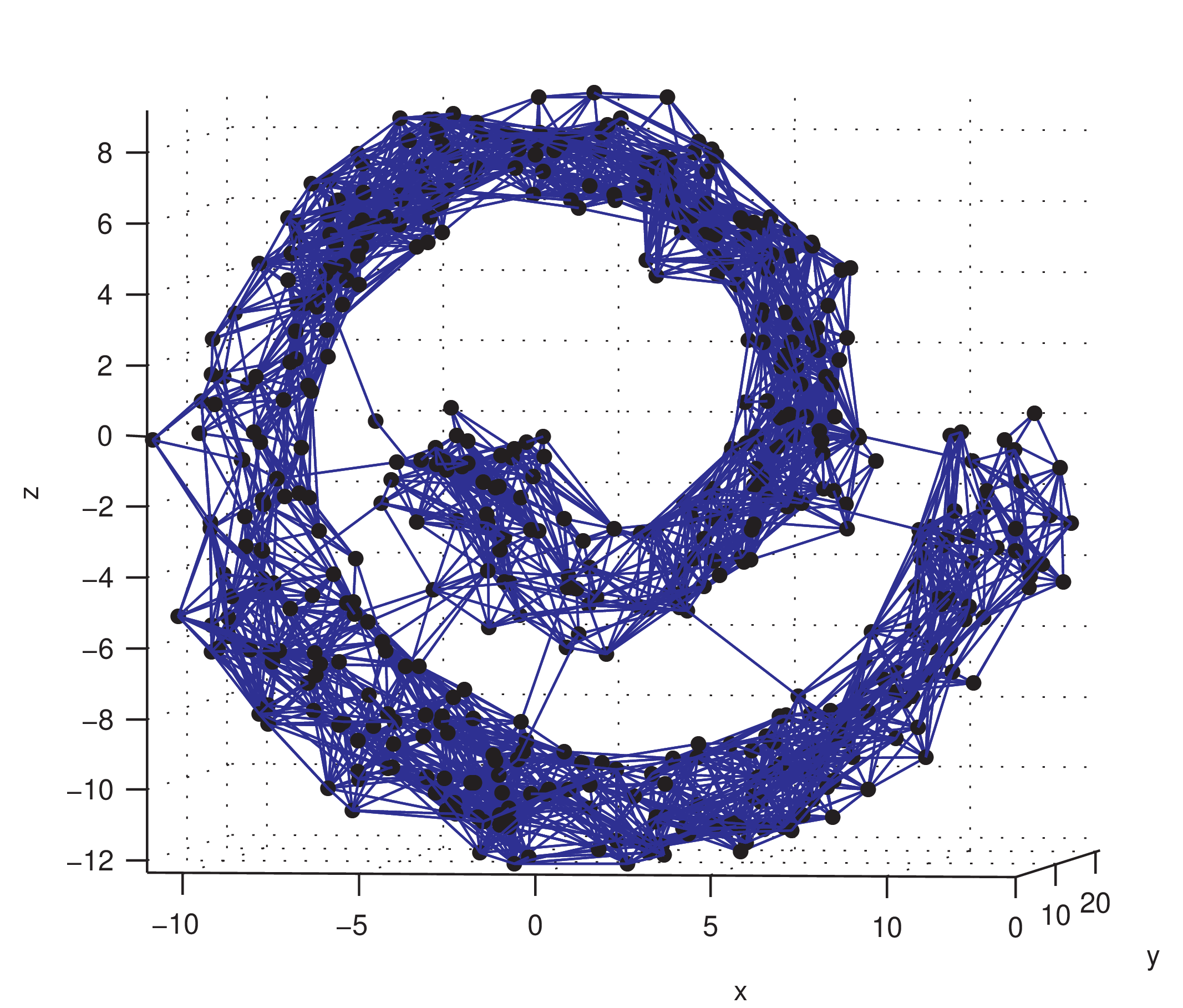
(a) NN graph of Swiss roll ($\mu$=1.6)

$\mu$	#B
1.23	0
1.28	2
1.44	10
1.54	20
1.64	32
1.74	46
1.85	66
1.90	76

(b) Median bridge count vs. $\mu$.

Figure 2.1: Noisy Swiss Roll

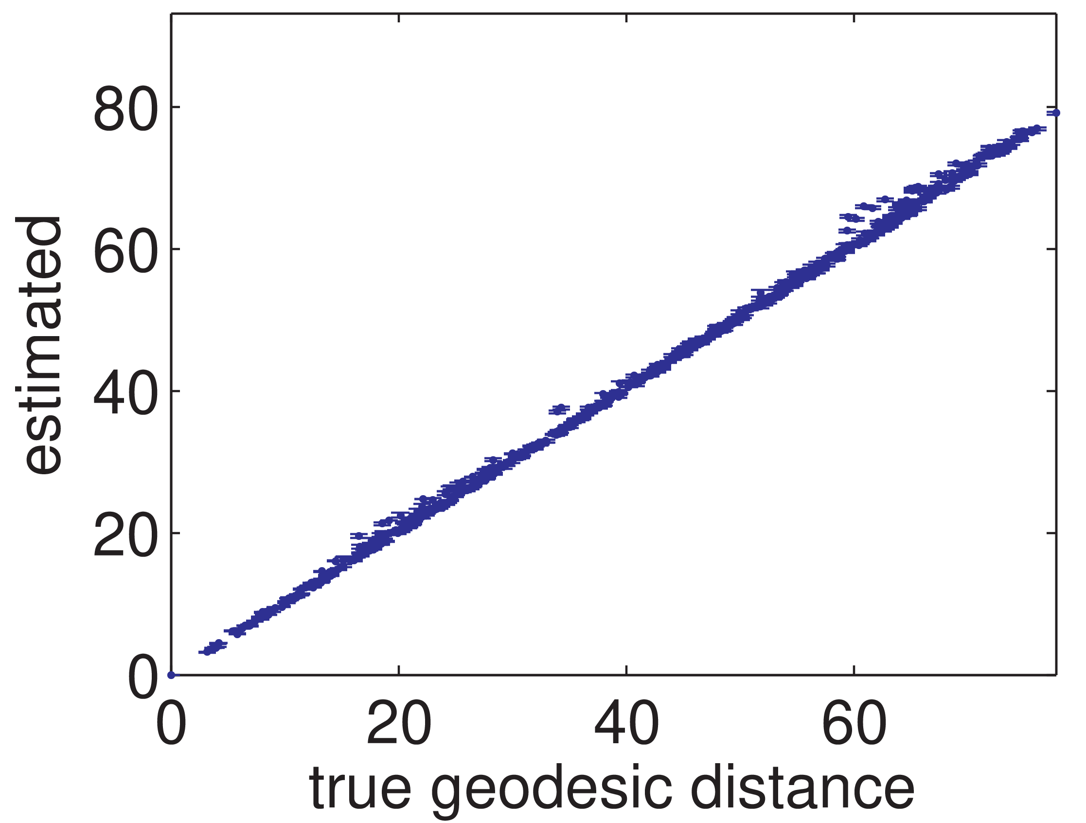
(a) $\mu=.1$

(b) $\mu=1.54$

Figure 2.2: SP Denoising: Swiss Roll Geodesic estimates vs. ground truth (from $x_{1}$)

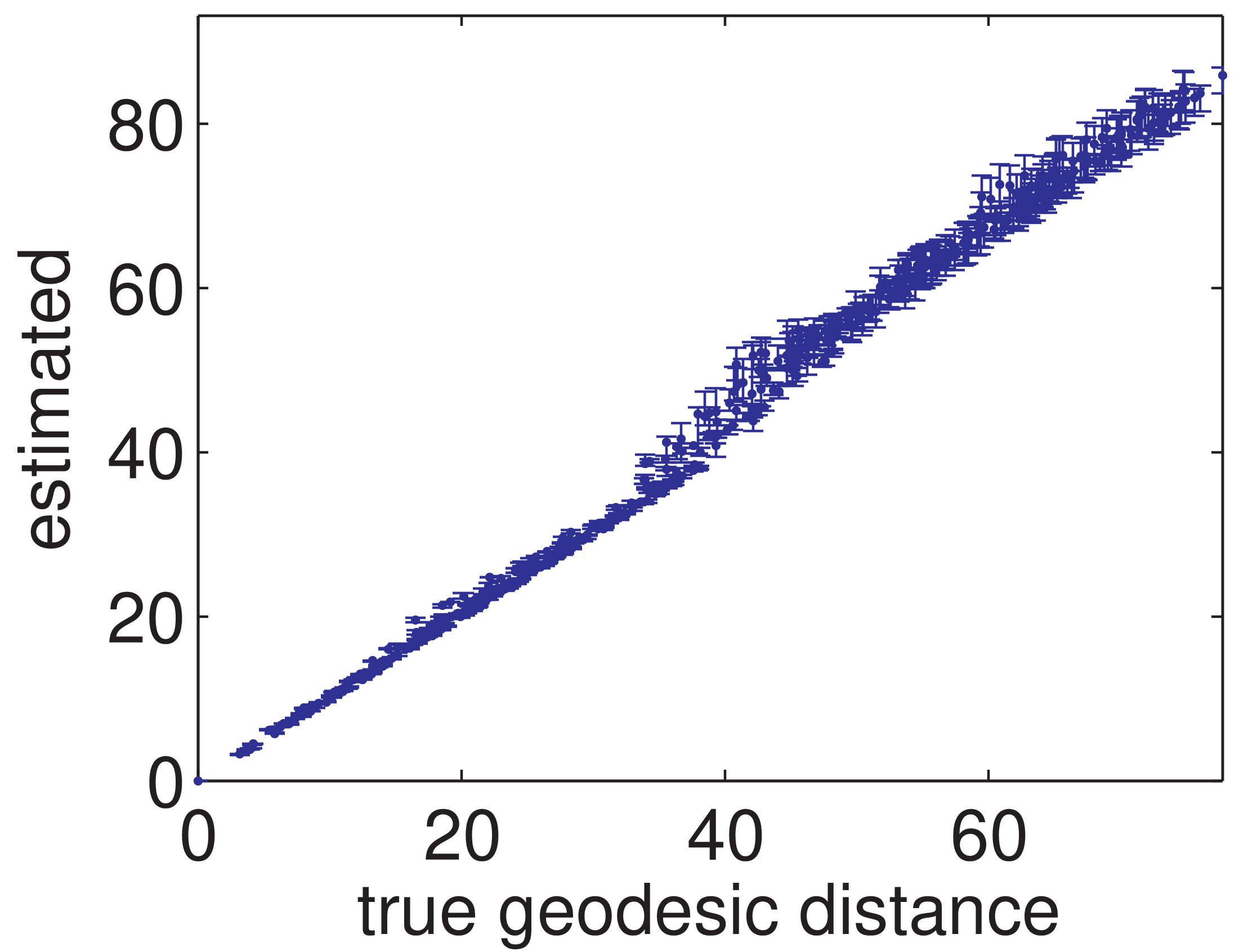
(a) $\mu=.1,q=.92$

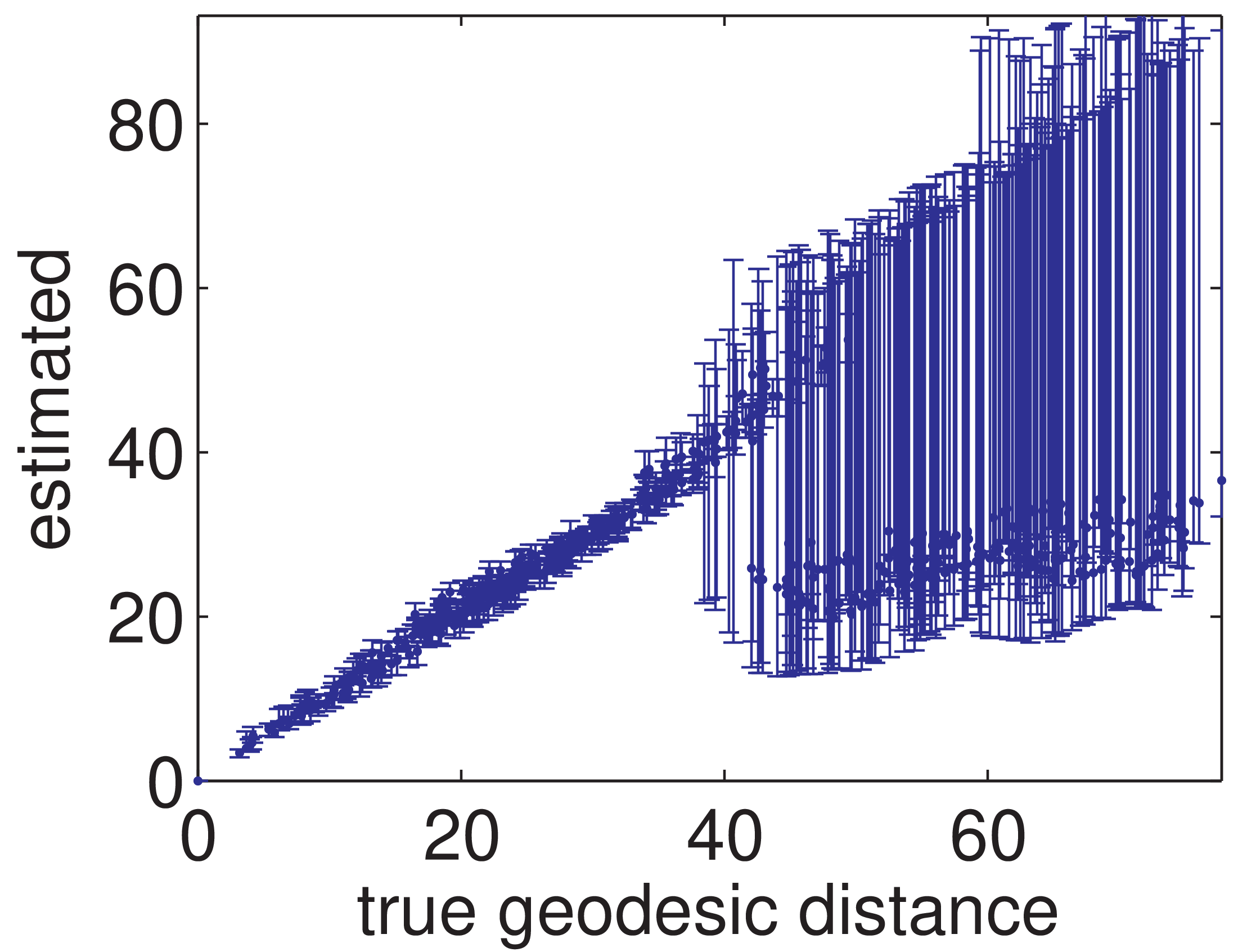
(b) $\mu=1.54,q=.92$

Figure 2.3: ECDR Denoising: Swiss Roll Geodesic estimates vs. ground truth (from $x_{1}$)

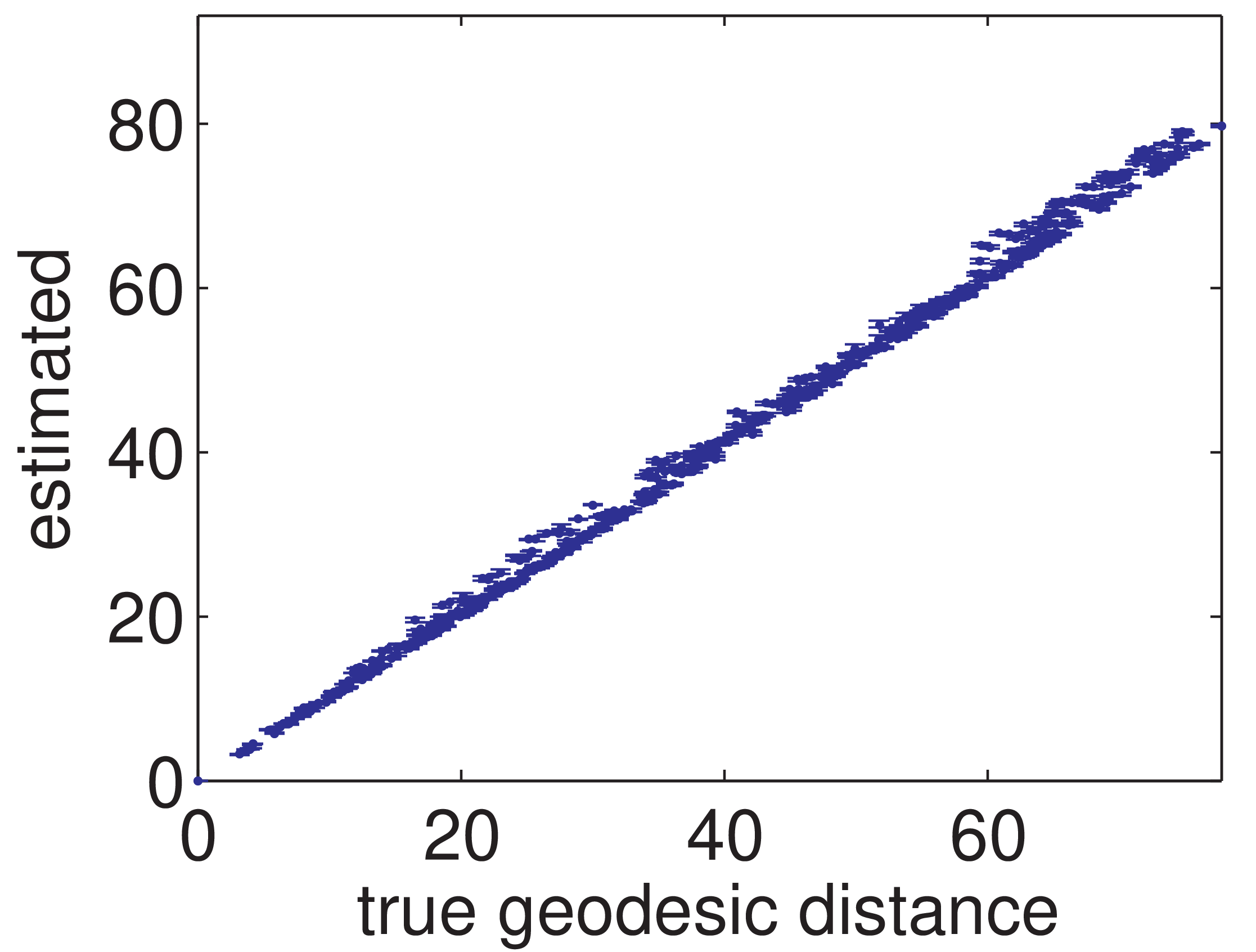
(a) $\mu=.1,q=.92$

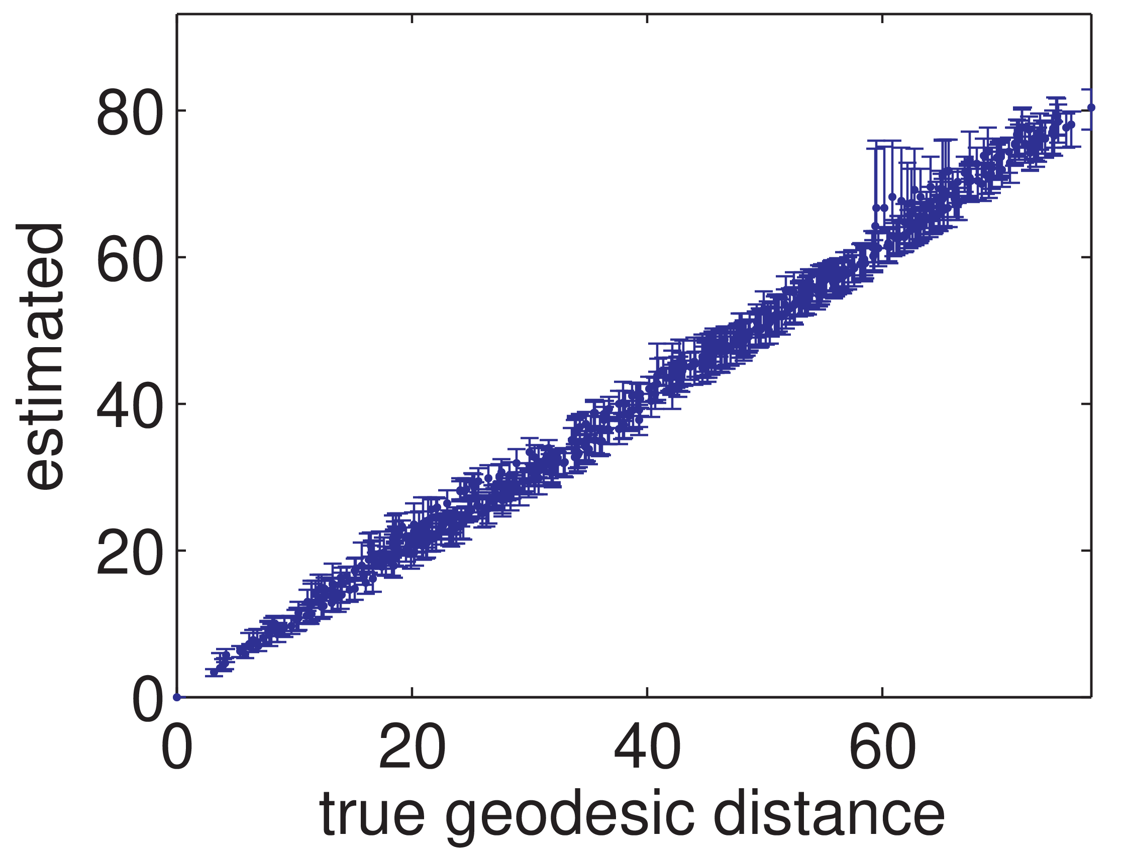
(b) $\mu=1.54,q=.92$

Figure 2.4: NPDR Denoising: Swiss Roll Geodesic estimates vs. ground truth (from $x_{1}$)

The initial NN graph $G$ was constructed using $\delta$-balls ($\delta=4$). The median bridge counts over $T$ realizations are shown in Fig. 2.1(b). Bridges first appear at $\mu\approx 1.2$. Fig. 2.1(a) shows one realization of ${\mathcal{Y}}$ and the NN graph $G$ (note bridges). We compare the simple SP with the LDR, ECDR ($K=15$), and NPDR ($p=0.01$) -based estimators by plotting the estimates of geodesic distance versus ground truth (sorted by distance from $x_{1}$). We plot the median estimate, 33%, and 66% quantiles over the $T$ runs, for $\mu=.1$ and $\mu=1.54$. The LDR and JDR based estimators’ performance is comparable to SP for $q>.9$ (plots not included).

With no noise: SP provides excellent estimates; NPDR estimates are accurate even after removing $8\%$ of the graph edges (Fig. 2.4(a)); however, ECDR removes important edges (Fig. 2.3(a)). At $\mu=1.54$ with approximately $25$ bridges: SP has failed (Fig. 2.2(b)); ECDR is removing bridges but also important edges, resulting in an upward estimation bias (Fig. 2.3(b)); in contrast, NPDR is successfully discounting bridges without any significant upward bias even at $q=.92$ (Fig. 2.4(b)). This supports our claim that bridges occur between edges with low neighbor probability in the NPDR random walk. Lower values of $q$ remove more edges, including bridges, but removing non-bridges always increases SP estimates, and can lead to an upward bias. The choice of $q$ should be based on prior knowledge of the noise or cross-validation.

Table 2.1: Comparison of mean error $E$, varying $\mu$.

$\mu$	SP	LDR,	ECDR, q=			NPDR, q=
		q=.92	.92	.95	.99	.92	.95	.99
0.10	0.8	1.5	4.4	3.8	1.9	2.4	1.9	1.2
1.44	12.0	10.9	10.7	8.1	2.1	3.6	2.5	1.6
1.54	13.6	12.8	11.7	7.6	2.5	3.8	2.6	2.3
1.64	14.4	13.9	11.6	6.8	5.1	4.0	3.1	6.5
1.74	14.9	14.4	11.4	6.5	8.9	5.0	5.6	11.1
1.85	15.3	14.9	12.1	8.6	12.0	8.1	9.4	13.4

Table 2.1 compares the performance of DRs at moderate noise levels. For this experiment, we chose $5$ points, $\left\{x_{r}\right\}_{r=1}^{5}$, well distributed over ${\mathcal{M}}$. Over $T=100$ noise realizations, we calculated the mean of the value

$$E=\frac{1}{5n}\sum_{r=1}^{5}\sum_{i=1}^{n}\left\lvert g_{ri}-{\tilde{g}}_{ri}\right\rvert,$$

the average absolute error of the geodesic estimate from all of the points to these 5. As seen in this figure, given an appropriate choice of $q$, NPDR outperforms the other DRs at moderate noise levels. As expected, $q$ must grow with the noise level as more bridges are found in the initial graph.

2.6 Denoising a Random Projection Graph

We now consider the random projection tomography problem of [96]. Random projections of $I$ are taken at angles $\theta\in[0,2\pi)$. More specifically, these projections are $f(\theta)=R_{\theta}(I)$, where $R_{\theta}$ is the Radon transform at angle $\theta$.

In [96], we observe $n=1024$ random projections:

$$y_{i}=f(\theta_{i})+\nu_{i}\qquad\text{where}\qquad\nu_{i}\sim N(0,\sigma^{2}).$$

for which the ambient dimension of the projection is $r=512$ and $\sigma^{2}=\sigma^{2}_{f}/10^{SNR_{db}/10}$, where the signal power is $\sigma_{f}^{2}\approx 0.0044$. The image used in all experiments is the Shepp-Logan phantom (Fig. 2.5(a)), and the projection angles are unknown (Fig. 2.5(b)). After some initial preprocessing, a NN graph ($k=50$) is constructed from the noisy projections, and JDR is used to detect bridges in this graph. After detected bridges are removed (pruned), nodes with less than two remaining edges (that is, isolated nodes) are removed from the graph. An eigenvalue problem on the new graph’s adjacency matrix is then solved to find an angular ordering of the remaining projections (nodes). Finally, $\hat{I}$ is reconstructed via an inverse Radon transform of these resorted projections.

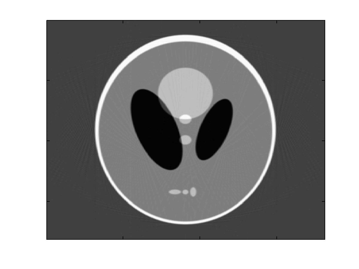
(a) Original Phantom, $I$

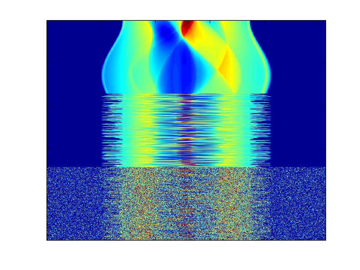
(b) Projections of $I$

Figure 2.5: Shepp-Logan Phantom and Radon Projections. In (b), the y-axis represents projection angle. The top third shows regularly ordered projections $f(\theta)$. The middle third shows projections when $\theta$ has been randomized. The lower third shows projections after angles have been randomized and noise has been added (SNR is -2db)

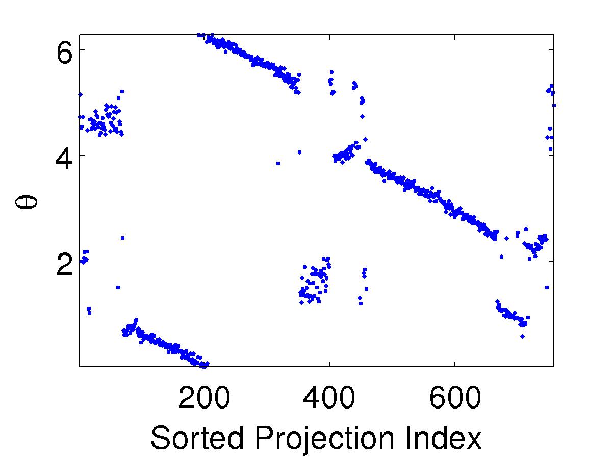
(a) Estimated $\theta$, JDR

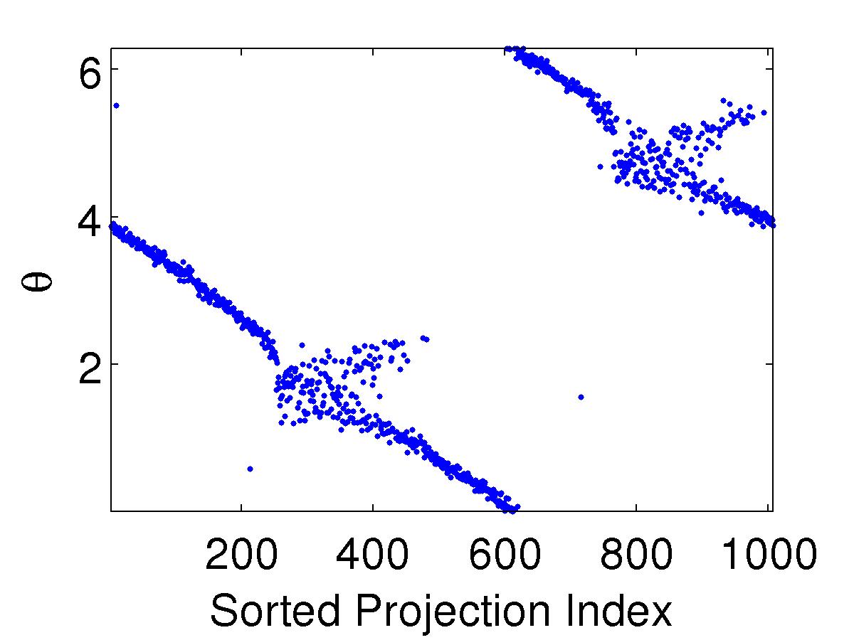
(b) Estimated $\theta$, NPDR

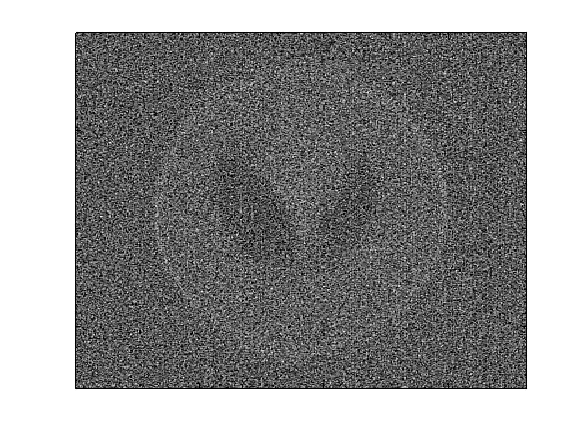
(c) Reconstruction $\hat{I}$, JDR

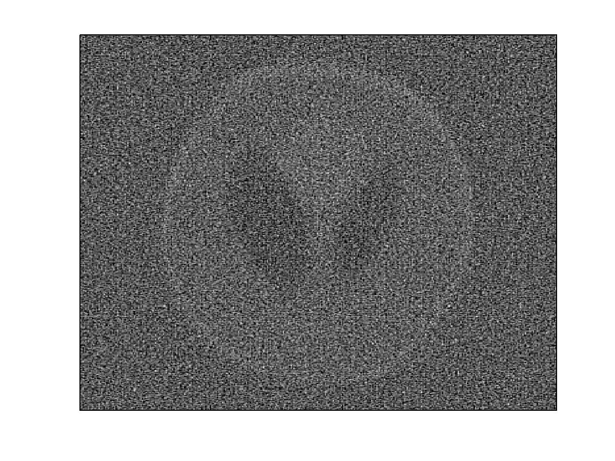
(d) Reconstruction $\hat{I}$, NPDR

Figure 2.6: Tomography Reconstructions from Random Projections

We compared JDR to NPDR pruning at a SNR of $-2\text{db}$. Exhaustive search finds the optimal $q$ for JDR at $q=.78$. For NPDR we used $\hat{P}_{\infty}$ (all edges in $G$ have weight $1$), $p=.01$, and $q=.8$. After pruning, JDR disconnected 277 nodes compared to 21 for NPDR. The estimated sorted angles are shown in Figs. 2.6(a),2.6(b), and the rotated reconstructions in Figs. 2.6(c),2.6(d). Under the similarity metric $\rho=\frac{I^{T}\hat{I}}{\left\lVert I\right\rVert\left\lVert\hat{I}\right\rVert}$, with alignment of $\hat{I}$ with $I$, the increase in NPDR similarity (0.15) over JDR similarity ($0.12$) is 25%. Note the clearer boundaries in the NPDR phantom, thanks to 256 additional (unpruned) projections (best viewed on screen). At moderate noise levels, NPDR removes fewer NN graph nodes and yields a more accurate reconstruction. As more projections are left after pruning, the final accuracy is higher.

2.7 Conclusion and Connections

We studied the problem of estimating geodesics in a point cloud. A slight revision for removing edges from a neighborhood graph allows us to avoid disconnecting weakly connected groups. Building on this framework, we studied several global measures for detecting topological bridges in the NN graph. In particular, we developed and analyzed the NPDR bridge detection rule, which is based on a special type of Markov random walk. Using a special random walk matrix derived from the geometry of the sample points, we constructed the NPDR to detect bridges by thresholding entries of the neighborhood matrix ${N_{\epsilon}}$. The entries of column $i$ in this matrix converge to those of a special averaging operator in the neighborhood of point $x_{i}$ in ${\mathcal{M}}$: the averaging intrinsically performed by the Laplace Beltrami operator around $x_{i}$.

Our experiments indicate that NPDR robustly detects bridges in the NN graph without misclassifying edges important for geodesic estimation or tomographic angle estimation. Furthermore, it does so over a wider noise range than competing methods, e.g. LDR and ECDR. It can be calculated efficiently via a sparse eigenvalue decomposition. Preliminary evidence from synthetic experiments indicates that, as §2.4 suggests, for NPDR one should choose $p$ as small as possible while retaining numerical conditioning of $I-{\bar{p}}{P_{\epsilon}}$.

For very large $n$ and small $\epsilon$, the matrices ${N_{\epsilon}}$ and ${P_{\epsilon}}$ are equivalent, but in practical cases ${N_{\epsilon}}$ yields significantly better performance. More testing of NPDR on non-synthetic datasets is needed. Possible applications include determining bridges in social and webpage (hyperlink) network graphs, and in the common line graphs estimated in the blind 3D tomography “Cryo-EM” problem [95].

Furthermore, the matrix ${N_{\epsilon}}$ is closely related to the regularized inverse of the graph Laplacian. The term ${P_{\epsilon}}-I$ in (2.5) is proportional to the weighted graph Laplacian ${L_{\epsilon}}$, and from this equation it is clear that ${N_{\epsilon}}$ is proportional to the inverse of the Tikhonov regularized weighted graph Laplacian (with regularization parameter $p/{\bar{p}}$). The efficacy of the NPDR, and the initial theoretical results developed in §2.4.1 lead us to study the regularized inverse of the graph Laplacian in more detail; this is the focus of Chapter 3.

Chapter 3 The Inverse Regularized Laplacian: Theory

3.1 Introduction

Semi-supervised learning (SSL) encompasses a class of machine learning problems in which both labeled data points and unlabeled data points are available during the training (fitting) stage [19]. In contrast to supervised learning, the goal of SSL algorithms is to improve future prediction accuracy by including information from the unlabeled data points during training. SSL extends a wide class of standard problems, such as classification and regression.

A number of recent nonlinear SSL algorithms use aggregates of nearest neighbor (NN) information to improve inference performance. These aggregates generally take the form of some transform, or decomposition, of the weighted adjacency, or weight, matrix of the NN graph. Formal definitions of NN graphs, and associated weight matrices, are given in §2.2; we will also review them in the SSL learning context in §3.3.1.

Motivated by several of these algorithms, we show a connection between a certain nonlinear transform of the NN graph weight matrix, the regularized inverse of the graph Laplacian matrix, and the solution to the regularized Laplacian partial differential equation (PDE), when the underlying data points are sampled from a compact Riemannian manifold. We then show a connection between this PDE and the Eikonal equation, which generates geodesics on the manifold.

These connections lead to intuitive geometric interpretations of learning algorithms whose solutions include a regularized inverse of the graph Laplacian. As we will show in chapter 4, it also enables us to build a robust geodesic distance estimator, a competitive new multiclass classifier, and a regularized version of ISOMAP.

This chapter is organized as follows: §3.3.1-§3.3.4 motivate our study by showing that in a certain limiting case, a standard SSL problem can be modeled as a regularized Laplacian (RL) PDE problem. §3.3.5-§3.3.8 derive the relationship between the regularized Laplacian and geodesics and discusses convergence issues as an important regularization term (viscosity) goes to zero.

3.2 Prior Work

The graph Laplacian is an important tool for regularizing the solutions of unsupervised and semi-supervised learning problems, such as classification and regression, in high-dimensional data analysis [101, 4, 6, 115, 65]. Similarly, estimating geodesic distances from sample points on a manifold has important applications in manifold learning and SSL (see, e.g., chapter 2 and [105, 20, 8]). Though heavily used in the learning and geometry communities, these methods still raise many questions. For example, with dimension $d>1$, graph Laplacian regularized SSL does not work as expected in the large sample limit [74]. It is also desirable to have geometric intuition about the behavior of the solutions of models like those proposed in [6, 115] in the limit when the data set is large.

To this end, we elucidate a connection between three important components of analysis of points sampled from manifolds:

1. The inverse of the regularized weighted graph Laplacian matrix.

2. A special type of elliptic Partial Differential Equation (PDE) on the manifold.

3. Geodesic distances on the manifold.

This connection provides a novel geometric interpretation for machine learning algorithms whose solutions require the regularized inverse of a graph Laplacian matrix. It also leads to a consistent geodesic distance estimator with two desired properties: the complexity of the estimator depends only on the number of sample points and the estimator naturally incorporates a smoothing penalty.

3.3 Manifold Laplacian, Viscosity, and Geodesics

We motivate our study by first looking at a standard semisupervised learning problem (§3.3.1). We show that as the amount of data increases and regularization is relaxed, this problem reduces to a PDE (§3.3.2-§3.3.3). We then analyze this PDE in the low regularization setting to uncover new geometric insights into its solution (§3.3.5-§3.3.7). In §3.3.9, these insights will allow us to analyze the original SSL problem from a geometric perspective.

3.3.1 A Standard SSL Problem

We present a classic SSL problem in which points are sampled, some with labels, and a regularized least squares regression is performed to estimate the labels on the remaining points. The regression contains two regularization penalties: a ridge regularization penalty and a graph Laplacian “smoothing” penalty.

Data points ${\mathcal{X}}=\left\{x_{i}\right\}_{i=1}^{n}$ are sampled from a space ${\mathcal{M}}\subset{\mathbb{R}}^{p}$. The first $l$ of these $n$ points have associated labels: $w_{i}\in{\mathcal{L}}\subset{\mathbb{R}},i=1,\ldots,l$. For binary classification, one could take ${\mathcal{L}}=\left\{\pm 1\right\}$. The goal is to find a vector ${\tilde{f}}\in{\mathbb{R}}^{n}$ that approximates the $n$ samples at the points in ${\mathcal{X}}$ of an unknown smooth function $f$ on ${\mathcal{M}}$ and minimizes the regression penalty $\sum_{i=1}^{l}(f(x_{i})-w_{i})^{2}$. The solution is regularized by two penalties: the ridge penalty $\|{\tilde{f}}\|_{2}$ and the graph Laplacian penalty $\widetilde{J}({\tilde{f}})={\tilde{f}}^{T}L{\tilde{f}}$; details of the construction of $L$ are given in §3.3.3. The second penalty approximately penalizes the gradient of $f$. It is a discretization of the functional: ${J(f)=\int_{{\mathcal{M}}}\left\lVert\nabla f(x)\right\rVert^{2}d{\mathcal{P}}(x)=\int_{{\mathcal{M}}}f(x)\Delta f(x)d{\mathcal{P}}(x),}$ where ${\mathcal{P}}(x)$ is the sampling density.

To find ${\tilde{f}}$ we solve the convex minimization problem:

$$\min_{{\tilde{f}}\in{\mathbb{R}}^{n}}\sum_{i=1}^{l}({\tilde{f}}_{i}-w_{i})^{2}+\gamma_{A}\|{\tilde{f}}\|^{2}_{2}+\gamma_{I}\widetilde{J}({\tilde{f}}),$$ (3.1)

where the nonnegative regularization parameters $\gamma_{A}$ and $\gamma_{I}$ depend on $l$ and $n$.

We can rewrite (3.1) in its matrix form. Let $E_{\mathcal{A}}=\text{diag}\left(1\cdots 1\ \ 0\cdots 0\right)$ have $l$ ones followed by $n-l$ zeros on its diagonal, and let $E_{\mathcal{A}^{\prime}}=I-E_{\mathcal{A}}$. Further, let $\widetilde{w}=\left[w_{1}\ \cdots\ w_{l}\ \ 0\ \cdots\ 0\ \right]^{T}$ be a vector of the labels $w_{i}$ for the first $l$ sample points, and zeros for the unlabeled points. Then Eq. (3.1) can be written as:

$$\min_{{\tilde{f}}\in{\mathbb{R}}^{n}}\|\widetilde{w}-E_{\mathcal{A}}{\tilde{f}}\|^{2}_{2}+\gamma_{A}{\tilde{f}}^{T}{\tilde{f}}+\gamma_{I}{\tilde{f}}^{T}L{\tilde{f}}$$ (3.2)

This is a quadratic program for ${\tilde{f}}$. Setting the gradient, with respect to ${\tilde{f}}$, to zero yields the linear system

$$\left(E_{\mathcal{A}}+\gamma_{A}I+\gamma_{I}L\right){\tilde{f}}=\widetilde{w}.$$ (3.3)

The optimization problem (3.1) and the linear system (3.3) are related to two previously studied problems. The first is graph regression with Tikhonov regularization [4]. Problem (3.3) is closely related to the one solved in Algorithm 1 of that paper, where we replace their general penalty $\gamma S$ term with the more specific form $\gamma_{A}I+\gamma_{I}L$. The ridge penalty $\gamma_{A}I$ encourages stability in the solution, replacing their zero-sum constraint on $f$. The second related problem is Laplacian Regularized Least Squares (LapRLS) of [6]. Specifically, (3.3) is identical to Eq. 35 of [6] with one of the regularization terms removed by setting the kernel matrix $K$ equal to the identity. In that framework, the matrix $K$ is defined as $K_{ij}\propto e^{-\left\lVert x_{i}-x_{j}\right\rVert^{2}/(2\sigma^{2})}$, $i,j=1,\ldots,n$ for some $\sigma>0$. A choice of $\sigma>0$ regularizes for finite sample size and sampling noise [6, Thm. 2, Remark 2]. Eq. (3.3) is thus closely related to the limiting solution to the LapRLS problem in the noiseless case, where the sampling size $n$ grows and $\sigma$ shrinks quickly with $n$.

We study the following problem: suppose the function $w$ is sampled without noise on specific subsets of ${\mathcal{M}}$. The estimate ${\tilde{f}}$ represents an extension of $w$ to the rest of ${\mathcal{M}}$. What does this extension look like, and how does it depend on the geometry of ${\mathcal{M}}$? The first step is to understand the implications of the noiseless case on (3.3); we study this next.

3.3.2 SSL Problem – Assumptions

We now list our main assumptions for the SSL problem in (3.3):

1. ${\mathcal{M}}$ is a $d$-dimensional ($d<p$) manifold $({\mathcal{M}},g)$, which is compact, and Riemannian.

2. The labeled points $\left\{x_{i}\right\}_{i=1}^{l}$ are sampled from a regular and closed nonempty subset ${\mathcal{A}}\subset{\mathcal{M}}$.

3. The labels $\left\{w_{i}\right\}_{i=1}^{l}$ are sampled from a smooth (e.g. $C^{2}$ or Lipschitz) function $w:{\mathcal{A}}\to{\mathcal{L}}\subset{\mathbb{R}}$.

4. The density ${\mathcal{P}}$ is nonzero everywhere on ${\mathcal{M}}$, including on ${\mathcal{A}}$.

These assumptions ensure that the points ${\mathcal{X}}$ are sampled without noise from a bounded, and smooth space, that the labels are sampled without noise, and that the label data is also sampled from a bounded and smooth function. We will use these assumptions to show the convergence of ${\tilde{f}}$ to a smooth function $f$ on ${\mathcal{M}}$.

In assumption 2 we use the term regular in the PDE sense [47, Irregular Boundary Point]; we discuss this further in §4.4. We call ${\mathcal{A}}$ the anchor set (or anchor); note that it is not necessarily connected. In addition, let ${\mathcal{A}^{\prime}}={\mathcal{M}}\backslash{\mathcal{A}}$ denote the complement set. In assumption 3, for $w$ to be smooth it suffices that it is smooth on all connected components of ${\mathcal{A}}$. Thus we can allow ${\mathcal{L}}$ to take on discrete values, as long as the classes they represent are separated from each other on ${\mathcal{M}}$. We call the function $w$ the anchor condition or anchor function. Note finally that assumption 4 implies that the labeled data size $l$ grows with $n$.

As we have assumed that there is no noise on the labels (assumptions 2 and 3), we will not apply a regularization penalty to the labeled data. On the labeled points, therefore, (3.3) reduces to $E_{\mathcal{A}}{\tilde{f}}=\widetilde{w}$. Hence, the regularized problem becomes an interpolation problem. The ridge penalty, now restricted to the unlabeled data, changes from ${\tilde{f}}^{T}{\tilde{f}}$ to ${\tilde{f}}^{T}E_{\mathcal{A}^{\prime}}{\tilde{f}}$. The Laplacian penalty function becomes ${J(f)=\int_{{\mathcal{A}^{\prime}}}f(x)\Delta f(x)d{\mathcal{P}}(x)}$, and the discretization of this penalty similarly changes from ${\tilde{f}}^{T}L{\tilde{f}}$ to $(E_{\mathcal{A}^{\prime}}{\tilde{f}})^{T}E_{\mathcal{A}^{\prime}}L{\tilde{f}}$. The original linear system (3.3) thus becomes

$$M_{n}{\tilde{f}}=\widetilde{w},$$ (3.4)

where $$M_{n}=E_{\mathcal{A}}+\gamma_{A}(n)E_{\mathcal{A}^{\prime}}+\gamma_{I}(n)E_{\mathcal{A}^{\prime}}L.$$

We note that the dimensions of $M_{n}$, ${\tilde{f}}$, and $\widetilde{w}$ in (3.4) grow with $n$.

A more detailed explanation of the component terms in the original problem (3.2) and the linear systems (3.3) and (3.4) are available in §3.4.2, where we show that the solution to the simplified problem (3.4) depends only on the ratio $\gamma_{I}(n)/\gamma_{A}(n)$. We will return to this in §3.3.3.

3.3.3 SSL Problem – the Large Sample Limit – Preliminary Results

We study the linear system (3.4) as $n\to\infty$, and prove that given an appropriate choice of graph Laplacian $L$ and growth rate of the regularization parameters $\gamma_{A}(n)$ and $\gamma_{I}(n)$, the solution ${\tilde{f}}$ converges to the solution $f$ of a particular PDE on ${\mathcal{M}}$. The convergence occurs in the $\ell_{\infty}$ sense with probability $1$.

Our proof of convergence has two parts. First, we must show that $M_{n}{\tilde{f}}$ models a forward PDE with increasing accuracy as $n$ grows large; this is called consistency. Second, we must show that the norm of $M_{n}^{-1}$ does not grow too quickly as $n$ grows large; this is called stability. These two results will combine to provide the desired proof. As all of our estimates rely on the choice of graph Laplacian matrix on the sample points ${\mathcal{X}}$, we first detail the specific construction that we use throughout:

1. Construct a weighted nearest neighbor (NN) graph $G=({\mathcal{X}},{\mathcal{E}},{\tilde{d}})$ from $k$-NN or $\delta$-ball neighborhoods of ${\mathcal{X}}$, where edge $(l,k)\in{\mathcal{E}}$ is assigned the distance ${\tilde{d}}_{lk}=\left\lVert x_{k}-x_{l}\right\rVert_{{\mathbb{R}}^{p}}$.

2. Choose $\epsilon>0$ and let $({\hat{P}_{\epsilon}})_{lk}=\exp(-{\tilde{d}}_{kl}^{2}/\epsilon)$ if $(l,k)\in{\mathcal{E}}$, $1$ if $l=k$, and $0$ otherwise.

3. Let ${\hat{D}_{\epsilon}}$ be diagonal with $({\hat{D}_{\epsilon}})_{kk}=\sum_{l}({\hat{P}_{\epsilon}})_{kl}$, and normalize for sampling density by setting ${A_{\epsilon}}={\hat{D}_{\epsilon}}^{-1}{\hat{P}_{\epsilon}}{\hat{D}_{\epsilon}}^{-1}$.

4. Let ${D_{\epsilon}}$ be diagonal with $({D_{\epsilon}})_{kk}=\sum_{l}({A_{\epsilon}})_{kl}$ and define the row-stochastic matrix ${P_{\epsilon}}={D_{\epsilon}}^{-1}{A_{\epsilon}}$.

5. The asymmetric normalized graph Laplacian is ${L_{\epsilon}}=(I-{P_{\epsilon}})/\epsilon$.

We will use ${L_{\epsilon}}$ from now on in place of the generic Laplacian matrix $L$.

Regardless of the sampling density, as $n\to\infty$ and $\epsilon(n)\to 0$ at the appropriate rate, ${L_{\epsilon}}$ converges (with probability 1) to the Laplace-Beltrami operator on ${\mathcal{M}}$: ${{L_{\epsilon}}\to-c\Delta}$, for some $c>0$, uniformly pointwise [48, 94, 23, 108] and in spectrum [5]. The concept of correcting for sampling density was first suggested in [60].

This convergence forms the basis of our consistency argument. We first introduce a result of [94], which shows that with probability 1, as $n\to\infty$, the system (3.4) with $L={L_{\epsilon}}_{(n)}$ consistently models the Laplace-Beltrami operator in the $\ell_{\infty}$ sense.

Let $\pi_{\mathcal{X}}:L^{2}({\mathcal{M}})\to{\mathbb{R}}^{n}$ map any square integrable function on the manifold to the vector of its samples on the discrete set ${\mathcal{X}}\subset{\mathcal{M}}$.

Theorem 3.3.1 (Convergence of ${L_{\epsilon}}$: [94], Eq. 1.7).

Suppose we are given a compact Riemannian manifold ${\mathcal{M}}$ and smooth function $f:{\mathcal{M}}\to{\mathbb{R}}$. Suppose the points ${\mathcal{X}}$ are sampled iid from everywhere on ${\mathcal{M}}$. Then, for $n$ large and $\epsilon$ small, with probability $1$

$$({L_{\epsilon}}\pi_{\mathcal{X}}(f))_{i}=-c\Delta f(x_{i})+O\left(\frac{1}{n^{1/2}\epsilon^{1/2+d/2}}+\epsilon\right),$$

where $\Delta$ is the negatively defined Laplace-Beltrami operator on ${\mathcal{M}}$, and $c>0$ is a constant. Choosing $\epsilon=Cn^{-1/(3+d/2)}$ (where $C$ depends on the geometry of ${\mathcal{M}}$) leads to the optimal bound of $O(n^{-1/(3+d/2)})$. Following [48], the convergence is uniform.

As convergence is uniform in Thm. 3.3.1, we may write the bound in terms that we will use throughout:

$$\left\lVert{L_{\epsilon}}\pi_{\mathcal{X}}(f)-c^{\prime}\pi_{\mathcal{X}}(\Delta f)\right\rVert_{\infty}=O(n^{-1/(3+d/2)}),$$ (3.5)

where $c^{\prime}=-c$ and $\left\lVert\cdot\right\rVert_{\infty}$ is the vector infinity norm.

We now show that $M_{n}$ (as defined in (3.4)) is consistent:

Corollary 3.3.2 (Consistency of $M_{n}$).

Assume that ${\partial{\mathcal{M}}}=\emptyset$ or that ${\partial{\mathcal{M}}}\subset{\mathcal{A}}$. Let $F_{n}$ be the following operator for functions $f\in C^{2}({\mathcal{A}^{\prime}})\cap C^{0}({\mathcal{A}})$:

$$F_{n}f(x)=\begin{cases}\gamma_{A}(n)f(x)-c\gamma_{I}(n)\Delta f(x)&x\in{\mathcal{A}^{\prime}}\\ f(x)&x\in{\mathcal{A}}\end{cases}$$ (3.6)

Then, under the same conditions as in Thm. 3.3.1, with probability $1$ for $n$ large and $\epsilon$ chosen as in Thm. 3.3.1, $\left\lVert M_{n}\pi_{\mathcal{X}}(f)-\pi_{\mathcal{X}}(F_{n}f)\right\rVert_{\infty}=O(n^{-1/(3+d/2)})$.

Proof.

This follows directly from Thm. 3.3.1 and the fact that $(E_{\mathcal{S}}f)_{i}=f(x_{i})\delta_{x_{i}\in{\mathcal{S}}}$ for any set ${\mathcal{S}}\subset{\mathcal{M}}$. ∎

Our notion of stability is described in terms of certain limiting inequalities. We use the notation $a_{n}<_{n}b_{n}$ to mean that there exists some $n_{0}$ such that for all $n^{\prime}>n_{0}$, $a_{n^{\prime}}<b_{n^{\prime}}$.

Proposition 3.3.3 (Stability of $M_{n}$).

Suppose that $\gamma_{I}(n)/\gamma_{A}(n)<_{n}\epsilon(n)/\kappa$, $\kappa>2$. Then $\left\lVert M_{n}^{-1}\right\rVert_{\infty}=O(\gamma_{A}^{-1}(n))$.

The proof of Prop. 3.3.3 is mainly technical and is given in §3.4.1.

If we modify $M_{n}$ as

$$M^{\prime}_{n}=E_{\mathcal{A}}+E_{\mathcal{A}^{\prime}}(I+h^{2}{L_{\epsilon}}),$$ (3.7)

we can also state the following corollary, which will be useful in chapter 4.

Corollary 3.3.4 (Stability of $M^{\prime}_{n}$).

Suppose $h^{2}(n)<_{n}\epsilon(n)/\kappa$, $\kappa>2$. Then $\left\lVert{M^{\prime}}_{n}^{-1}\right\rVert_{\infty}=O(1)$.

3.3.4 SSL Problem – the Large Sample Limit – Convergence Theorem

We are now ready to state and prove our main theorem about the convergence of ${\tilde{f}}$. We assume that ${\mathcal{M}}$ has empty boundary, or that ${\partial{\mathcal{M}}}\subset{\mathcal{A}}$. For the case of nonempty manifold boundary ${\partial{\mathcal{M}}}\not\subset{\mathcal{A}}$, there are additional constraints at this boundary in the resulting PDE. We discuss this case in §3.4.3. Note, by assumption 2 of §2, the anchor set ${\mathcal{A}}$ and its boundary $\partial{\mathcal{A}}$ are not empty.

Theorem 3.3.5 (Convergence of ${\tilde{f}}$ under $M_{n}$).

Consider the solution of $M_{n}{\tilde{f}}_{n}=\widetilde{w}$ (Eq. (3.4) with $L={L_{\epsilon}}$), with ${\mathcal{M}}$, ${\mathcal{A}}$, and $w$ as described in §3.3.2, and with either ${\partial{\mathcal{M}}}=\emptyset$ or ${\partial{\mathcal{M}}}\subset{\mathcal{A}}$. Further, assume that

1. $\epsilon(n)$ shrinks as given in Thm. 3.3.1.

2. $\lim_{n\to\infty}\epsilon(n)/\gamma_{A}(n)=0$.

3. As in Prop. 3.3.3, $\gamma_{I}(n)<_{n}\gamma_{A}(n)\epsilon(n)/\kappa$ for some $\kappa>2$.

Then for $n$ large, with probability 1,

$$\left\lVert{\tilde{f}}_{n}-\pi_{\mathcal{X}}f_{n}\right\rVert_{\infty}<_{n}\epsilon(n)/\gamma_{A}(n)$$

where the function $f_{n}\in C^{2}({\mathcal{M}})$ is the unique, smooth, solution to the following PDE for the given $n$:

$$f_{n}(x)-c\frac{\gamma_{I}(n)}{\gamma_{A}(n)}\Delta f_{n}(x)=0,\quad x\in{\mathcal{A}^{\prime}}\qquad\text{and}\qquad f_{n}(x)=w(x),\quad x\in{\mathcal{A}}.$$ (3.8)

Proof of Thm. 3.3.5, Convergence.

Let $F_{n}$ be given by (3.6) and let $f_{n}$ be the solution to (3.8). The existence and uniqueness of $f_{n}$, under assumptions 1-3 of §3.3.2, is well known (we show it in §3.3.5).

We bound $\left\lVert{\tilde{f}}_{n}-\pi_{\mathcal{X}}f_{n}\right\rVert_{\infty}$ as follows:

$$\left\lVert{\tilde{f}}_{n}-\pi_{\mathcal{X}}f_{n}\right\rVert_{\infty} =\left\lVert M_{n}^{-1}\widetilde{w}-\pi_{\mathcal{X}}f_{n}\right\rVert_{\infty}$$

$$=\left\lVert M_{n}^{-1}(\pi_{\mathcal{X}}(F_{n}f_{n})-M_{n}\pi_{\mathcal{X}}f_{n})\right\rVert_{\infty}$$

$$\leq\left\lVert M_{n}^{-1}\right\rVert_{\infty}\left\lVert\pi_{\mathcal{X}}(F_{n}f_{n})-M_{n}\pi_{\mathcal{X}}f_{n}\right\rVert_{\infty}.$$

From stability (Prop. 3.3.3), $\left\lVert M_{n}^{-1}\right\rVert_{\infty}=O(\gamma_{A}^{-1}(n))$, and by consistency (Cor. 3.3.2), with probability 1 for large $n$, $\left\lVert\pi_{\mathcal{X}}(F_{n}f_{n})-M_{n}\pi_{\mathcal{X}}f_{n}\right\rVert_{\infty}=O(\epsilon(n))$.

The theorem follows upon applying assumption 2. ∎

If we modify $M_{n}$ in Thm. 3.3.5 as in (3.7), we obtain Cor. 3.3.6 below.

Corollary 3.3.6 (Convergence of ${\tilde{f}}^{\prime}$ under $M^{\prime}_{n}$).

Consider the solution of $M^{\prime}_{n}{\tilde{f}}_{n}^{\prime}=\widetilde{w}$, with ${\mathcal{M}}$, ${\mathcal{A}}$, and $w$ as described in §3.3.2, and with $\partial{\mathcal{M}}=\emptyset$ or ${\partial{\mathcal{M}}}\subset{\mathcal{A}}$. Further, assume $\epsilon(n)$ shrinks as given in Thm. 3.3.1, and $h(n)$ as in Cor. 3.3.4. Then for $n$ large, with probability 1,

$$\left\lVert{\tilde{f}}_{n}^{\prime}-\pi_{\mathcal{X}}f_{n}\right\rVert_{\infty}=O(\epsilon(n))$$

where $f_{n}\in C^{2}({\mathcal{M}})$ again solves (3.8):

$$f_{n}(x)-h^{2}(n)\Delta f_{n}(x)=0,\quad x\in{\mathcal{A}^{\prime}}\qquad\text{and}\qquad f_{n}(x)=w(x),\quad x\in{\mathcal{A}}.$$

Proof of Cor. 3.3.6.

Similar to that of Thm. 3.3.5, with stability given by Cor. 3.3.4. ∎

We will call (3.8) the Regularized Laplacian PDE (RL PDE) with the regularization parameter $h(n)=\sqrt{c\gamma_{I}(n)/\gamma_{A}(n)}$. By assumptions 1 and 2 of Thm. 3.3.5 , $h(n)\to 0$ as $n\to\infty$. This, and the analysis in §3.3.2, motivate us to study the RL PDE when $h$ is small to gain some insight into its solution, and hence into the behavior of the original SSL problem.

3.3.5 The Regularized Laplacian PDE

We now study the RL PDE in greater detail. We will assume a basic knowledge of differential geometry on compact Riemannian manifolds throughout. For basic definitions and notation, see App. A.

We rewrite the RL PDE (3.8), now denoting the explicit dependence on a parameter $h$, and making the problem independent of sampling:

$$-h^{2}\Delta f_{h}(x)+f_{h}(x)=0\quad x\in{\mathcal{A}^{\prime}}\qquad\text{and}\qquad f_{h}(x)=w(x)\quad x\in{\mathcal{A}},$$ (3.9)

where ${\mathcal{M}}$, ${\mathcal{A}}$, and $w$ are defined as in §3.3.2. The idea is that $f_{h}$ is specified smoothly on ${\mathcal{A}}$ and by solving (3.9) we seek a smooth extension of $f_{h}$ to all of ${\mathcal{M}}$.

The RL PDE, (3.9), has been well studied [109, Thm. 6.22], [54, App. A]. It is uniformly elliptic, and for $h>0$ it admits a unique, bounded, solution ${f_{h}\in C^{2}({\mathcal{A}^{\prime}})\cap C^{0}({\mathcal{M}})}$. The boundedness of $f_{h}$ follows from the strong maximum principle [109, Thm. 3.5]. One consequence is that $f_{h}$ will not extrapolate beyond an interval determined by the anchor values.

Proposition 3.3.7 ([54], §A.2).

The RL PDE (3.9) has a unique, smooth solution that is bounded within the range $(w_{-},w_{+})$ for $x\in{\mathcal{A}^{\prime}}$, where

$$w_{-}=\inf_{y\in{\mathcal{A}}}\min(w(y),0)\qquad\text{and}\qquad w_{+}=\sup_{y\in{\mathcal{A}}}\max(w(y),0).$$

Our goal is to understand the solution of (3.9) as the regularization term vanishes, i.e., $h\downarrow 0$. To do so, we introduce the Viscous Eikonal Equation.

3.3.6 The Viscous Eikonal Equation

The RL PDE is closely related to what we will call the Viscous Eikonal (VE) equation. This is the following “smoothed” Hamilton-Jacobi equation of Eikonal type:

$$-h\Delta S_{h}(x)+\left\lVert\nabla S_{h}(x)\right\rVert^{2}=1\quad x\in{\mathcal{A}^{\prime}}\qquad\text{and}\qquad S_{h}(x)=u_{h}(x)\quad x\in{\mathcal{A}}.$$ (3.10)

The term containing the Laplacian is called the viscosity term, and $h$ is called the viscosity parameter.

The two PDEs, (3.9) and (3.10), are connected via the following proposition:

Proposition 3.3.8.

Consider (3.9) with $h>0$ and $w(x)>0$, and (3.10) with $u_{h}(x)=-h\log w(x)$. When solution $f_{h}$ exists for (3.9), then $S_{h}=-h\log f_{h}$ is the unique, smooth, bounded solution to (3.10).

Proof.

Let $f_{h}$ be the unique solution of (3.9). From Prop. 3.3.7, $f_{h}>0$ for $x\in{\mathcal{A}^{\prime}}$. Apply the inverse of the smooth monotonic bijection $\tau_{h}(t)=e^{-t/h}$, $\tau_{h}:[0,\infty)\to(0,1]$ to $f_{h}$. Let $R_{h}=-h\log f_{h}$, hence $f_{h}=e^{-R_{h}/h}$.

We will need the standard product rule for the divergence “$\nabla\cdot$”. When $f$ is a differentiable function and $\bm{f}$ is a differentiable vector field,

$$\nabla\cdot(f\bm{f})=(\nabla f)\cdot\bm{f}+(\nabla\cdot\bm{f})f.$$ (3.11)

As $f_{h}$ is harmonic, on ${\mathcal{A}^{\prime}}$:

$$0 =-h^{2}\nabla\cdot\nabla e^{-R_{h}/h}+e^{-R_{h}/h}$$ (3.12)

$$=h\nabla\cdot(e^{-R_{h}/h}(\nabla R_{h}))+e^{-R_{h}/h}$$ (3.13)

$$=h(\nabla e^{-R_{h}/h}\cdot\nabla R_{h}+e^{-R_{h}/h}\nabla\cdot\nabla R_{h})+e^{-R_{h}/h}$$ (3.14)

$$=e^{-R_{h}/h}(-\left\lVert\nabla R_{h}\right\rVert^{2}+h\Delta R_{h}+1).$$ (3.15)

Here, from (3.12) to (3.13) we use the chain rule, and from (3.13) to (3.14) we use the product rule (3.11). After dropping the positive multiplier in (3.15), we see that that $R_{h}$ satisfies the first part of (3.10). Further, $R_{h}\in C^{2}({\mathcal{A}^{\prime}})\cap C^{0}({\mathcal{M}})$ because $\tau_{h}$ is a smooth bijection. Similarly, $R_{h}$ is bounded because $f_{h}$ is: ${R_{h}\in[-h\log w_{+},-h\log w_{-})}$.

Finally, on the boundary ${\mathcal{A}}$ we have $e^{-R_{h}/h}=w$, equivalently $R_{h}=-h\log w$. Hence, $R_{h}$ solves (3.10).

∎

To summarize: for $h>0$, (3.10) has a unique solution $S_{h}\in C^{2}({\mathcal{A}^{\prime}})$ (Prop. 3.3.8; see also [109, 54]).

We are interested in the solutions of the VE Eq. for the case of $h=0$ as well as for solutions obtained for $h>0$ small and for more general $u_{h}$. When $h=0$ and $u_{h}=0$, it is well known that on a compact Riemannian manifold ${\mathcal{M}}$, (3.10) models propagation from ${\mathcal{A}}$ through ${\mathcal{A}^{\prime}}$ along shortest paths. Results are known for a number of important cases, and we will discuss them after describing the following assumption.

Assumption 3.3.1.

For $h=0$ and $u_{0}$ sufficiently regular, (3.10) has the unique viscosity solution:

$$S_{0}(x)=\inf_{y\in{\mathcal{A}}}\left(d(x,y)+u_{0}(y)\right),$$ (3.16)

where $d(x,y)$ is the geodesic distance between $x$ and $y$ through ${\mathcal{A}^{\prime}}$. Furthermore, as $h\to 0$, $S_{h}$ converges to $S_{0}$ in $L^{p}({\mathcal{A}^{\prime}})$, $1\leq p<\infty$, and in $(L^{\infty}({\mathcal{A}^{\prime}}))^{*}$ (i.e. essentially pointwise) when $u_{h}$ converges to $u_{0}$ in the same sense. The rate of convergence is $\left\lVert S_{0}-S_{h}\right\rVert_{\infty}^{*}=O(h)$.

From now on we will denote $S_{0}$ simply by $S$.

Discussion of Assum. 3.3.1 on compact ${\mathcal{M}}$.

To our knowledge, a complete proof of (3.16) for compact Riemannian ${\mathcal{M}}$ is not known; the theory of unique viscosity solutions (nondifferentiable in some areas), on manifolds is an open area of research [26, 2]. However, below we cite known partial results.

Eq. (3.16) was shown to hold for $u_{0}=0$ on compact ${\mathcal{M}}$ in [68, Thm. 3.1], and for $u_{0}$ sufficiently regular on bounded, smooth, and connected subsets of ${\mathbb{R}}^{d}$ in [64, Thms. 2.1, 6.1, 6.2], and e.g., when $u_{0}$ is Lipschitz [58, Eq. 4.23]. Convergence and the convergence rate of $S_{h}$ to $S_{0}$ were also shown on such Euclidean subsets in [64, Eq. 69]. Conditions of convergence to a viscosity solution are not altered under the exponential map [2, Cor. 2.3], thus convergence in local coordinates around ${\mathcal{A}}$ (which follows from [64, Thm. 6.5] and Prop. 3.3.8) implies convergence on open subsets of ${\mathcal{A}^{\prime}}$. However, global convergence of $S_{h}$ to $S_{0}$ on ${\mathcal{M}}$ is still an open problem.

Not surprisingly, despite the lack of formal proof, and in light of the above evidence, our numerical experiments on a variety of nontrivial compact Riemannian manifolds (e.g. compact subsets of hyperbolic paraboloids) give additional evidence that this convergence is achieved. ∎

3.3.7 What happens when $h$ converges to $0$: Transport Terms

To study the relationship between $S_{h}$ and $S$, we look for a higher order expansion of $f_{h}$ using a tool called Transport Equations [87].

Assume $f_{h}$ can be expanded into the following form:

$$f_{h}(x)=e^{-R(x)/h}\sum_{k\geq 0}h^{\alpha k}Z_{k}(x)$$ (3.17)

with $\alpha>0$. The terms $Z_{k}$, $k=0,1,\ldots$ are called the transport terms. Substitution of this form into (3.9) will give us the conditions required on $R$ and $Z_{k}$.

Theorem 3.3.9.

If (3.17), (with $\alpha=1$) is a solution to the RL PDE (3.9) for all $h>0$, then:

$$\forall x\in{\mathcal{A}}\text{ and }\forall k\geq 1\qquad R(x)=0,\qquad Z_{0}(x)=w(x),\qquad Z_{k}(x)=0,$$ (3.18)

and (3.9) reduces to a series of PDEs:

$$0 =-\left\lVert\nabla R\right\rVert^{2}+1$$

$$0 =Z_{0}\Delta R+2\nabla R\cdot\nabla Z_{0}$$ (3.19)

$$0 =Z_{k}\Delta R+2\nabla R\cdot\nabla Z_{k}-\Delta Z_{k-1},\quad k>0$$

In particular, letting $d_{\mathcal{A}}(x)=\inf_{y\in{\mathcal{A}}}d(x,y)$ denote the shortest geodesic distance from $x$ to ${\mathcal{A}}$, we have that $R(x)=d_{\mathcal{A}}(x)$ everywhere.

Proof.

The anchor conditions follow from the fact that for all $h>0$, $w=Z_{0}e^{-R/h}+hZ_{1}e^{-R/h}+\ldots$ (thus forcing $R=0$ and therefore $Z_{0}=w$, and $Z_{k}=0,\forall k>0$).

Plugging (3.17) into (3.9), and applying the product and chain rules, we get

$$0=\sum_{k\geq 0}e^{-R/h}h^{k}\left(-h^{2}\Delta Z_{k}+2h\nabla R\cdot\nabla Z_{k}+hZ_{k}\Delta R-Z_{k}\left\lVert\nabla R\right\rVert^{2}+Z_{k}\right).$$

Eqs. (3.19) follow after collecting like powers of $h$ and simplifying. ∎

Thm. 3.3.9 shows first that $R$ is determined by the Eikonal equation with zero boundary conditions. Second, it shows that $Z_{0}$ is the dominant term affected by the boundary values $w$ as $h{\downarrow}0$. For $k>0$, the transport terms $Z_{k}$ are affected by $w$ via $Z_{k-1}$, but these are not the dominant terms for small $h$. The existence, uniqueness, and smoothness of $Z_{0}$ on ${\mathcal{A}^{\prime}}$ and within the cut locus of ${\mathcal{A}}$, is proved in §3.4.1 (Thm. 3.4.4).

Note that the choice of $\alpha=1$ is not arbitrary. For $\alpha<1$ in (3.17), (3.9) does not admit a consistent set of solvable transport equations. For $\alpha=2$, the resulting transport equations reduce to those of Eqs. (3.19) (the nonzero odd $k$ terms are forced to zero and the even $k$ terms are related to each other via Eqs. (3.19)).

3.3.8 Manifold Laplacian and Vanishing Viscosity

We now combine Assum. 3.3.1 and Thm. 3.3.9 in a way that summarizes the solution of the RL PDE (3.9) for small $h$, taking into account possible arbitrary nonnegative boundary conditions.

Theorem 3.3.10.

Let $w(x)\geq 0,\forall x\in{\mathcal{A}}$ and let $\hat{{\mathcal{A}}}=\text{supp}\left(w\right)$. Further, define $f^{*}_{h}(x)=w(x^{\prime})e^{-d_{{\mathcal{A}}}(x)/h}$ where $x^{\prime}=\arg\inf_{y\in{\mathcal{A}}}d(x,y)$. Then for a situation where Assum. 3.3.1 holds, and for small $h>0$, the solution of (3.9) with sufficiently regular anchor ${\mathcal{A}}$, satisfies:

$$\left\lvert f_{h}(x)-f^{*}_{h}(x)\right\rvert =O(he^{-d_{\mathcal{A}}(x)/h});\text{and}$$ (3.20)

$$\lim_{h\to 0}-h\log f_{h}(x) =d_{\hat{{\mathcal{A}}}}(x).$$ (3.21)

Proof.

First, apply Thm. 3.3.9 to decompose $f_{h}$ in terms of $R$ and the transport terms $Z_{k}$, $k\geq 0$. Next, by Thm. 3.1 of [68], as discussed in Assum. 3.3.1, we obtain $R(x)=d_{{\mathcal{A}}}(x)$. We can therefore write $f_{h}(x)=Z_{0}(x)e^{-d_{\mathcal{A}}(x)/h}+O(he^{-d_{\mathcal{A}}(x)/h})$. Further, $Z_{0}(x)$ is unique and smooth within an intersection of ${\mathcal{A}}^{\prime}$ and a cut locus of ${\mathcal{A}}$, and satisfies the boundary conditions ($Z_{0}(x)=w(x)$ for $x\in{\mathcal{A}}$) . This can be shown using the method of characteristics (Thm. 3.4.4). This verifies (3.20).

Showing that (3.21) holds requires more work due to possible zero boundary conditions on ${\mathcal{A}}$. To prove (3.21), we find a sequence of PDEs, parametrized by viscosity $h$ and “height” $c>0$; we denote these solutions $\hat{f}_{h,c}(x)$. These solutions match $f_{h}$ as $h\to 0$. We then show that for large $c$, they also match $f_{h}$ for nonzero $h$.

Let $\hat{{\mathcal{A}}}(c,h)=\left\{x\in{\mathcal{A}}:w(x)>e^{-c/h}\right\}$ and ${\mathcal{A}}_{0}(c,h)=\left\{x\in{\mathcal{A}}:w(x)\leq e^{-c/h}\right\}$. We define $\hat{f}_{h,c}$ as the solution to (3.9) with the modified boundary conditions

$$w_{h,c}(x)=\begin{cases}w(x)&x\in\hat{{\mathcal{A}}}(c,h)\\ e^{-c/h}&x\in{\mathcal{A}}_{0}(c,h)\end{cases}.$$ (3.22)

This is a modification of the original problem with a lower bound saturation point of $e^{-c/h}$. Clearly, as $h\to 0$, $w_{h,c}(x)\to w(x)$ on the boundary.

As in Prop. 3.3.8, for fixed $c$ we can write $w_{h}(x)=e^{-u_{h}(x)/h}$ for any $x\in{\mathcal{A}}$ and $h>0$. Then

$$u_{h}(x)=\begin{cases}c&x\in{\mathcal{A}}_{0}(c,h)\\ -h\log w(x)&x\in\hat{{\mathcal{A}}}(c,h)\end{cases}.$$

Let ${\mathcal{A}}_{0}=\left\{x\in{\mathcal{A}}:w(x)=0\right\}$ and $\hat{{\mathcal{A}}}=\left\{x\in{\mathcal{A}}:w(x)>0\right\}$, and define

$$u_{0}(x)=\begin{cases}c&x\in{\mathcal{A}}_{0}\\ 0&x\in\hat{{\mathcal{A}}}\end{cases}.$$

Then

$$u_{h}(x)-u_{0}(x)=\begin{cases}0&w(x)=0\\ c&0<w(x)\leq e^{-c/h}\\ -h\log w(x)&w(x)>e^{-c/h}\end{cases}.$$

As $w(x)$ is regular and ${\mathcal{A}}$ is compact, $u_{h}\to u_{0}$ pointwise on ${\mathcal{A}}$, and the convergence is also uniform. Clearly, then, $u_{h}\to u_{0}$ almost everywhere on ${\mathcal{A}}$. Furthermore, for any $h>0$, $u_{h}\leq c$ everywhere on ${\mathcal{A}}$. Therefore $u_{h}\to u_{0}$ in $L^{p}$ for all $p\geq 1$ [59, Prop. 6.4]. The rate of convergence, $O(h)$, is determined by the set of points $\left\{x:w(x)>e^{-c/h}\right\}$. Thus, by Prop. 3.3.8 and Assum. 3.3.1,

$$\hat{S}_{0,c}(x)=\lim_{h\to 0}-h\log\hat{f}_{h,c}(x)=\min\left(d_{\hat{{\mathcal{A}}}}(x),c+d_{{\mathcal{A}}_{0}}(x)\right).$$ (3.23)

To match the boundary conditions of $\hat{f}_{h,c}$ to those of $f_{h}$ for a fixed $h>0$, we must choose $c$ large in (3.22). Subsequently, when $c$ is large in (3.23), e.g., when $c\geq\text{diam}({\mathcal{M}})$, we have $\hat{S}_{0,c}(x)=d_{\hat{{\mathcal{A}}}}(x)$. This verifies (3.21). ∎

When $w(x)=1$ on ${\mathcal{A}}$, and for small $h$, the exponent of $f_{h}$ directly encodes $d_{\mathcal{A}}$. The following simple example illustrates Thm. 3.3.10. Additional examples on the Torus $T=S^{1}{\times}S^{1}$ and on a complex triangulated mesh are included in §4.8 of chapter 4.

Example 3.3.1 (The Annulus in ${\mathbb{R}}^{2}$).

Let ${\mathcal{M}}=\left\{r_{0}\leq r\leq 1\right\}$, where $r=\left\lVert x\right\rVert$ is the distance to the origin. Let ${\mathcal{A}}=\left\{r=r_{0}\right\}\cup\left\{r=1\right\}$ be the inner and outer circles. Letting $w=1$ ($u_{h}=0$), we get $S(r)=d_{{\mathcal{A}}}(r)=\min(1-r,r-r_{0})$. For symmetry reasons, we can assume a radially symmetric solution to the RL Eq. For a given dimension $d$, the radial Laplacian is $\Delta f(r)=f^{\prime\prime}(r)+(d-1)r^{-1}f^{\prime}(r)$. So (3.9) becomes: $-h^{2}\left(f_{h}^{\prime\prime}(r)+r^{-1}f_{h}^{\prime}(r)\right)+f_{h}(r)=0$ for $r\in(r_{0},1)$, and $f_{h}(r_{0})=f_{h}(1)=1$. The solution, as calculated in Maple [72], is

$$f_{h}(r)=\frac{I_{0}(r/h)K_{0}(1/h)-I_{0}(r/h)K_{0}(r_{0}/h)-K_{0}(r/h)I_{0}(1/h)+K_{0}(r/h)I_{0}(r_{0}/h)}{K_{0}(1/h)I_{0}(r_{0}/h)-K_{0}(r_{0}/h)I_{0}(1/h)},$$

where $I_{j}$ and $K_{j}$ are the $j$’th order modified Bessel functions of the first kind and second kind, respectively. A series expansion of $f_{h}(r)$ around $h=0$ (partially calculated with Maple) gives

$$f_{h}(r)=\sqrt{r_{0}/r}e^{-(r-r_{0})/h}+\sqrt{1/r}e^{-(1-r)/h}+O(h)$$ (3.24)

As the limiting behavior of $f_{h}$, as $h$ grows small, depends on the exponents of the two terms in (3.24), one can check that the limit depends on whether $r$ is nearer to $r_{0}$ or $1$. Depending on this, one of the terms drops out in the limit. From here, it is easy to check that $\lim_{h\to 0}-h\log f_{h}(r)=S(r)$, confirming (3.21).

We simulated this problem with $r_{0}=0.25$ by sampling $n=1500$ points from the ball $B(0,1.25)$, rescaling points having $r\in[0,0.25)$ to $r=0.25$, and rescaling points having $r\in(1,1.25]$ to $r=1$. $S_{h}$ is approximated up to a constant using the numerical discretization, via (3.7), of (3.8). For the graph Laplacian we used a $k=20$ NN graph and $\epsilon=0.001$.

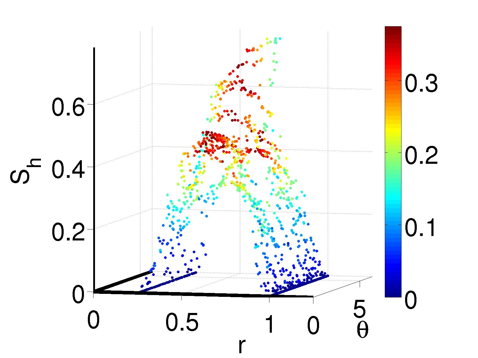
Figure 3.1: Geodesics Estimates $S_{h}(r,\theta)$ on Annulus. Left to Right: $h=1,\ 0.1,\ 0.001$.

Fig. 3.1 shows (in the $z$ axis) the estimate $S_{h}(x)$ as $h$ grows small. The colors of the points reflect the true distance to ${\mathcal{A}}$: $S(r)=S_{0}(r)=\min(1-r,r-r_{0})$. Note the convergence as $h{\downarrow}0$, and also the clear offset of $S_{h}$ which is especially apparent in the right panel at $r=0.25$ and $r=1$.

From the second of Eqs. (3.19) and the fact that $\nabla S(r)=1,\Delta S(r)=1/r$, we have $Z_{0}/r+2Z^{\prime}_{0}=0$ for $r_{0}<r\leq 1$, and $Z_{0}=1$ for $r\in\left\{r_{0},1\right\}$. To solve this near $r=r_{0}$, we use the boundary condition $Z_{0}(r_{0})=1$ and get $Z_{0}(r)=\sqrt{r_{0}/r}$. Likewise, near $r=1$ we use the boundary condition $Z_{0}(1)=1$ and get $Z_{0}(r)=\sqrt{1/r}$. Near $r=r_{0}$, the solution becomes $f_{h}(r)=e^{-(r-r_{0})/h}(\sqrt{r_{0}/r}+O(h))$, and near $r=1$, it becomes $f_{h}(r)=e^{-(1-r)/h}(\sqrt{1/r}+O(h))$, which match the earlier series expansion of the full solution. Furthermore, upon an additional Taylor expansion near $r=r_{0}$, we have $S_{h}(r)=r-r_{0}-h\log(r_{0}/r)/2+O(h\log h)$. Note the extra term in the $S_{h}$ estimate, which has a large effect when $r-r_{0}$ is small (as seen in the right pane of Fig. 3.1). A similar expansion can be made around the outer circle, at $r=1$.

3.3.9 The SSL Problem of §3.3.1, Revisited

Armed with our study of the RL PDE, we can now return to the original SSL problem of §3.3.1.

Suppose the anchor is composed of two simply connected domains ${\mathcal{A}}_{0}$ and ${\mathcal{A}}_{1}$, where $w$ takes on the constant values $c_{0}$ and $c_{1}$, respectively, within each domain. When $c_{1}>c_{0}\geq 0$, we can directly apply the result of Thm. 3.3.10 to (3.8). The solution, for $\gamma_{I}\ll\gamma_{A}$, is given by (3.20) with $h=\sqrt{c\gamma_{I}/\gamma_{A}}$:

$$f(x)\approx w(x^{\prime})\sup_{y\in{\mathcal{A}}}{e^{-d(x,y)\sqrt{\gamma_{A}/c\gamma_{I}}}}\qquad\text{where}\qquad x^{\prime}=\arg\inf_{y\in{\mathcal{A}}}d(x,y)$$

The solution depends on both the geometry of ${\mathcal{M}}$ (via the geodesic distance to ${\mathcal{A}}_{0}$ or ${\mathcal{A}}_{1}$) and on the values chosen to represent the class labels. For example, suppose ${\mathcal{L}}=\left\{0,1\right\}$. As $n$ grows large and $h$ grows small, we apply (3.21) to see that the classifier is biased towards the class in ${\mathcal{A}}_{0}$:

$$f(x)\approx\sup_{y\in{\mathcal{A}}_{1}}e^{-d(x,y)\sqrt{\gamma_{A}/c\gamma_{I}}}.$$ (3.25)

Choosing the symmetric labels ${\mathcal{L}}=\left\{c_{0},-c_{0}\right\}$ is more natural. In this case, we decompose (3.9) into two problems:

$$-h^{2}\Delta f_{h,0}+f_{h,0} =0\quad x\in{\mathcal{A}^{\prime}}\qquad\text{and}\qquad f_{h,0}=c_{0}\quad x\in{\mathcal{A}}_{0};\quad f_{h,0}=0\qquad x\in{\mathcal{A}}_{1}$$

$$-h^{2}\Delta f_{h,1}+f_{h,1} =0\quad x\in{\mathcal{A}^{\prime}}\qquad\text{and}\qquad f_{h,1}=0\ \quad x\in{\mathcal{A}}_{0};\quad f_{h,1}=-c_{0}\quad x\in{\mathcal{A}}_{1},$$

and note that by linearity of the problem and the separation of the anchor conditions, the solution to (3.9) is given by $f_{h}=f_{h,0}+f_{h,1}$. Therefore, by taking $h=\sqrt{c\gamma_{I}/\gamma_{A}}$, we separate (3.8) into two problems with nonnegative anchor conditions (one in $f_{h,0}$ and one in $-f_{h,1}$). Applying the result of Thm. 3.3.10 to each of these individually, and combining the solutions, yields

$$f(x)\approx c_{0}\sup_{y\in{\mathcal{A}}_{0}}e^{-d(x,y)/h}-c_{0}\sup_{y\in{\mathcal{A}}_{1}}e^{-d(x,y)/h}\propto e^{-d_{{\mathcal{A}}_{0}}(x)/h}-e^{-d_{{\mathcal{A}}_{1}}(x)/h}.$$ (3.26)

This solution is zero when $d_{{\mathcal{A}}_{0}}(x)=d_{{\mathcal{A}}_{1}}(x)$, positive when $d_{{\mathcal{A}}_{0}}(x)<d_{{\mathcal{A}}_{1}}(x)$, and negative otherwise. That is, in the noiseless, low regularization regime with symmetric anchor values, algorithms like LapRLS classification assign the point $x$ to the class that is closest in geodesic distance. We illustrate this with a simple example of classification on the sphere $S^{2}$.

Example 3.3.2.

We sample $n=1000$ points from the sphere $S^{2}$ at random, and define the two anchors ${\mathcal{A}}_{0}=B_{g}((1,0,0),\pi/16)$ and ${\mathcal{A}}_{1}=B_{g}((-1,0,0),\pi/16)$. Here $B_{g}(x,\theta)$ is a cap of angle $\theta$ around point $x$. The associated anchor labels are $w_{0}=+1$ and $w_{1}=-1$. We discretize the Laplacian ${L_{\epsilon}}$ using $k=50$, and $\epsilon=0.001$ and solve (3.4). Fig. 3.2 compares the numerical solutions at small $h$ to our estimates from (3.26). The two solutions are comparable up to a positive multiplicative factor (due to the fact that ${L_{\epsilon}}$ converges to $\Delta$ times a constant). $\square$

(a) $f_{h}$ on ${\mathcal{M}}$, numerical, log scale

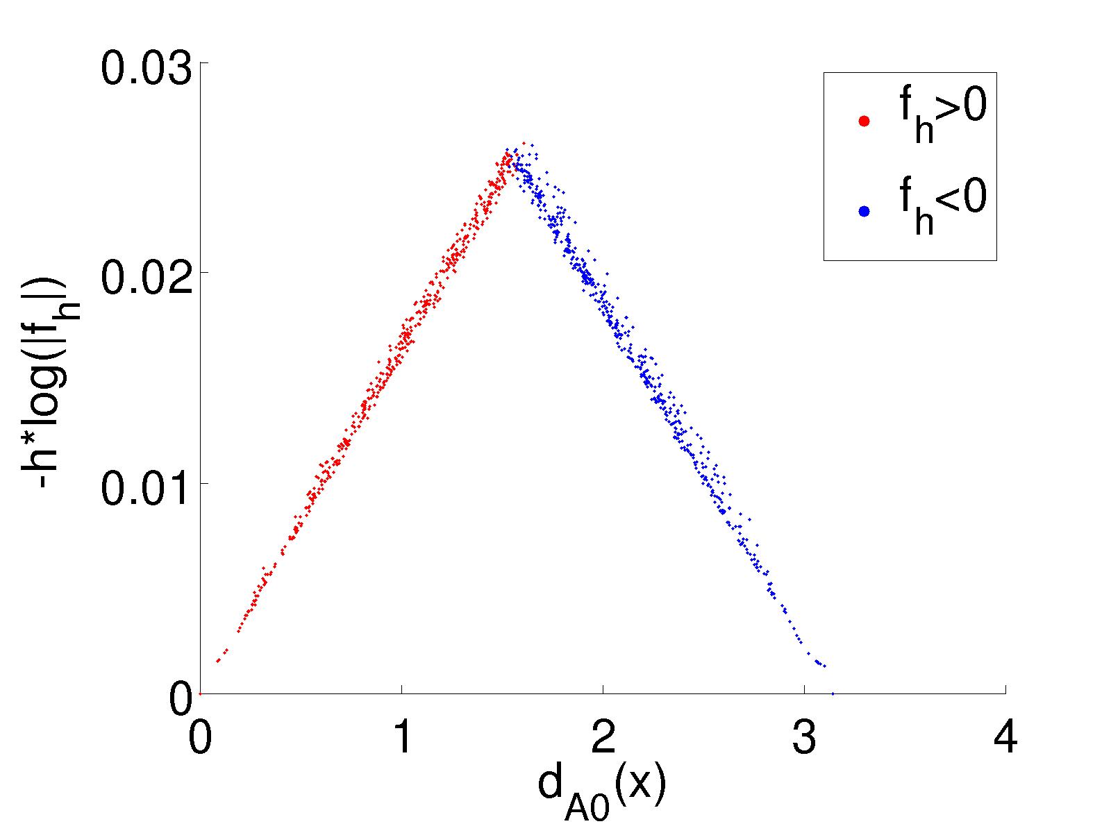
(b) $S_{h}$ (numerical)

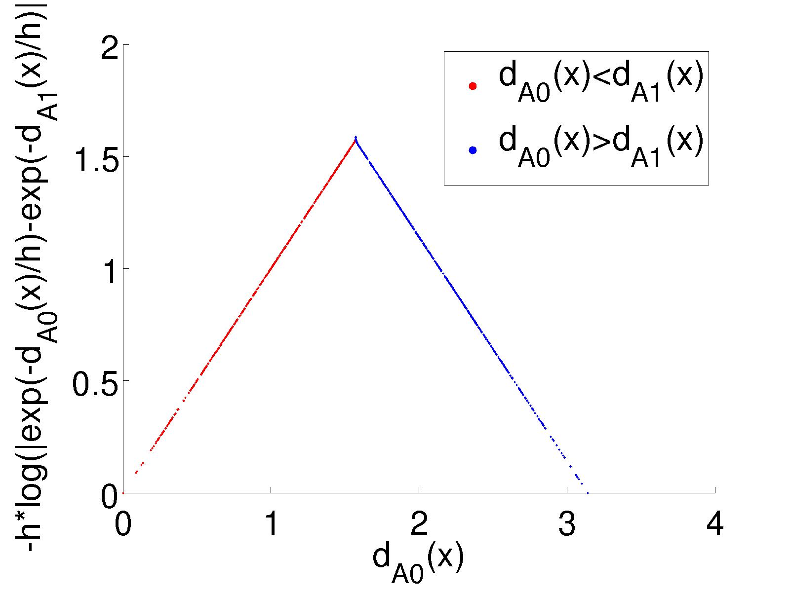
(c) $S_{h}$ (prediction)

Figure 3.2: Comparing solution of (3.4) to model prediction (3.26). Colors in (3.2(a)), are given by $-h\operatorname*{sign}(f_{h})\log\left\lvert f_{h}\right\rvert$; in (3.2(b)), encode $\operatorname*{sign}(f_{h})$; in (3.2(c)), encode closeness of $x$ to ${\mathcal{A}}_{0}$ vs. ${\mathcal{A}}_{1}$.

3.4 Technical Details

3.4.1 Deferred Proofs

Stability of $M_{n}$

To prove the stability of $M_{n}$, we first need to present some notation. The matrices ${P_{\epsilon}},{L_{\epsilon}},$ and ${D_{\epsilon}}$ can be written in terms of submatrices to simplify the exposition. Separating these matrices into submatrices associated with the $l$ labeled points and the $n-l$ unlabeled points, we write:

$${P_{\epsilon}} =\begin{pmatrix}P_{ll}&P_{lu}\\ P_{ul}&P_{uu}\end{pmatrix},\quad{L_{\epsilon}}=\begin{pmatrix}L_{ll}&L_{lu}\\ L_{ul}&L_{uu}\end{pmatrix}=\frac{1}{\epsilon}\begin{pmatrix}I-P_{ll}&-P_{lu}\\ -P_{ul}&I-P_{uu}\end{pmatrix},\quad$$

$$\text{and }{D_{\epsilon}} =\begin{pmatrix}D_{ll}&0\\ 0&D_{uu}\end{pmatrix}.$$

Note that the two identities in the definition of ${L_{\epsilon}}$ are of size $l$ and $n-l$, respectively.

We will also also need a lemma bounding the spectrum of the matrix $I-P_{uu}$.

Lemma 3.4.1.

The matrix $I-P_{uu}$ is bounded in spectrum between $0$ and $1$.

Proof.

The hermitian matrix $\tilde{P}_{\epsilon}={D_{\epsilon}}^{-1/2}{A_{\epsilon}}{D_{\epsilon}}^{-1/2}$ has eigenvalues bounded between $0$ and $1$. The eigenvalues of its lower right principal submatrix, $\tilde{P}_{uu}$, are therefore also bounded between $0$ and $1$ [49, Thm. 4.3.15]. Finally, $P_{uu}$ is similar to $\tilde{P}_{uu}$ via the transformation $P_{uu}=D_{uu}^{-1/2}\tilde{P}_{uu}D_{uu}^{1/2}$. ∎

We are now ready to prove the stability of $M_{n}$.

Proof of Prop. 3.3.3, Stability.

We first expand $M_{n}$ in block matrix form:

$$M_{n}=\begin{pmatrix}I&0\\ \gamma_{I}L_{ul}&G_{n}\end{pmatrix}\quad\text{where}\quad G_{n}=\gamma_{A}(n)I+\gamma_{I}(n)L_{uu}.$$

From the block matrix inverse formula, the inverse of $M_{n}$ is:

$$M_{n}^{-1}=\begin{pmatrix}I&0\\ -G_{n}^{-1}\gamma_{I}L_{ul}&G_{n}^{-1}\end{pmatrix},$$

and the norm may be bounded as:

$$\left\lVert M_{n}^{-1}\right\rVert_{\infty}\leq\max\left(1,\left\lVert G_{n}^{-1}\gamma_{I}L_{ul}\right\rVert_{\infty}+\left\lVert G_{n}^{-1}\right\rVert_{\infty}\right)$$ (3.27)

where we use the inequalities $\left\lVert(A^{T}\ B^{T})^{T}\right\rVert_{\infty}=\max(\left\lVert A\right\rVert_{\infty},\left\lVert B\right\rVert_{\infty})$ and $\left\lVert(C\ \ D)\right\rVert_{\infty}\leq\left\lVert C\right\rVert_{\infty}+\left\lVert D\right\rVert_{\infty}$.

We first expand $G_{n}^{-1}=(\gamma_{A}(n)I+\gamma_{I}(n)L_{uu})^{-1}=\gamma_{A}^{-1}(n)\left(I+\frac{\gamma_{I}}{\gamma_{A}\epsilon(n)}(I-P_{uu})\right)$. By Lem. 3.4.1, $I-P_{uu}$ is bounded in spectrum between $0$ and $1$, and by the first assumption in the proposition, when $\kappa>2$ we have $\gamma_{I}<_{n}\gamma_{A}\epsilon(n)/\kappa<_{n}\gamma_{A}(n)\epsilon(n)$. Thus there exists some $n_{0}$ so that for all $n^{\prime}>n_{0}$ we can write

$$G_{n}^{-1}=\gamma_{A}^{-1}(n)\left(I+\frac{\gamma_{I}(n)}{\gamma_{A}(n)\epsilon(n)}(I-P_{uu})\right)^{-1}=\gamma_{A}^{-1}\sum_{k=0}^{\infty}\left(\frac{\gamma_{I}(n)}{\gamma_{A}(n)\epsilon(n)}\right)^{k}(P_{uu}-I)^{k}.$$

Now we use this expansion to bound $\left\lVert G_{n}^{-1}\right\rVert_{\infty}$. Let $a_{n}=\gamma_{I}(n)(\gamma_{A}(n)\epsilon(n))^{-1}$. As the norm is subadditive,

$$\left\lVert G_{n}^{-1}\right\rVert_{\infty}\leq\gamma_{A}^{-1}(n)\sum_{k\geq 0}a^{k}_{n}\left\lVert P_{uu}-I\right\rVert_{\infty}^{k}.$$ (3.28)

Furthermore, we can bound $\left\lVert P_{uu}-I\right\rVert_{\infty}^{k}$ as follows. Since the entries of $P_{uu}$ are nonnegative, $\left\lVert P_{uu}-I\right\rVert_{\infty}\leq\left\lVert(P_{uu}+I)1\right\rVert_{\infty}$ where $1$ is a vector of all ones. Further, since $P_{uu}$ is a submatrix of a stochastic matrix, $\left\lVert(P_{uu}+I)1\right\rVert_{\infty}\leq 2$. Thus since $a_{n}=\gamma_{I}(n)(\gamma_{A}(n)\epsilon(n))^{-1}<_{n}\kappa^{-1}<1/2$, for $n$ large enough (3.28) is bounded by the geometric sum:

$$\left\lVert G_{n}^{-1}\right\rVert_{\infty}\leq\gamma_{A}^{-1}(n)\sum_{k\geq 0}(2a_{n})^{k}=\frac{1}{\gamma_{A}(n)(1-2a_{n})}=\frac{\epsilon(n)}{\epsilon(n)\gamma_{A}(n)-2\gamma_{I}(n)}$$

and this last term is bounded based on our initial assumption: $\epsilon(n)(\epsilon(n)\gamma_{A}(n)-2\gamma_{I}(n))^{-1}<_{n}\gamma_{A}^{-1}(n)(1-2\kappa^{-1})^{-1}$. Thus, for large enough $n$, $\left\lVert G_{n}^{-1}\right\rVert_{\infty}\leq\gamma_{A}^{-1}(n)(1-2\kappa^{-1})^{-1}$.

Now we bound $\left\lVert G_{n}^{-1}\gamma_{I}L_{ul}\right\rVert_{\infty}$. Note that $\left\lVert G_{n}^{-1}\gamma_{I}(n)L_{ul}\right\rVert_{\infty}\leq\gamma_{I}(n)\left\lVert G_{n}^{-1}\right\rVert_{\infty}\left\lVert L_{ul}\right\rVert_{\infty}$. As $L_{ul}=-P_{ul}$ and ${P_{\epsilon}}$ is stochastic, $\left\lVert L_{ul}\right\rVert_{\infty}\leq 1$. Putting together these two steps, we have $\left\lVert G_{n}^{-1}\gamma_{I}(n)L_{ul}\right\rVert_{\infty}\leq\gamma_{I}(n)\left\lVert G_{n}^{-1}\right\rVert_{\infty}$.

Combining these two bounds, (3.27) finally becomes

$$\left\lVert M_{n}^{-1}\right\rVert_{\infty}\leq\max{\left(1,\gamma_{A}(n)^{-1}(1-2\kappa^{-1})^{-1}(1+\gamma_{I}(n))\right)}.$$

For small $\gamma_{A}(n)>0$, the second term is the maximum and the result follows. ∎

Characterization of $Z_{0}$

We first need some preliminary definitions and results.

We define the cut locus of the set ${\mathcal{A}}$ as closure of the set of points in ${\mathcal{A}^{\prime}}$ where $d_{\mathcal{A}}^{2}(x)$ is not differentiable (i.e., where there is more than one minimal geodesic between $x$ and ${\mathcal{A}}$):

$$\operatorname*{Cut}({\mathcal{A}})=\overline{\left\{x\in{\mathcal{A}^{\prime}}\ |\ d_{\mathcal{A}}^{2}\text{ is not differentiable at }x\right\}}.$$

The cut locus and $d_{\mathcal{A}}$ have several important properties, which we now list:

1. The Hausdorff dimension of $\operatorname*{Cut}({\mathcal{A}})$ is at most $d-1$ [68, Cor. 4.12].

2. $\operatorname*{Cut}({\mathcal{A}})\cup{\mathcal{A}}$ is closed in ${\mathcal{M}}$.

3. The open set ${\mathcal{A}^{\prime}}\backslash\operatorname*{Cut}({\mathcal{A}})$ can be continuously retracted to $\partial{\mathcal{A}}$.

4. If ${\mathcal{A}}\in C^{r}$ then $d_{\mathcal{A}}$ is $C^{r}$ in ${\mathcal{A}^{\prime}}\backslash\operatorname*{Cut}({\mathcal{A}})$.

Items 2-4 are proved in [68, Prop 4.6].

Property 1 shows that $d_{\mathcal{A}}$ is smooth almost everywhere on ${\mathcal{A}^{\prime}}$. Properties 2-3 show that ${\mathcal{A}^{\prime}}\backslash\operatorname*{Cut}({\mathcal{A}})$ is composed of a finite number of disjoint connected components, each touching ${\mathcal{A}}$. Finally, property 4 shows that $d_{\mathcal{A}}$ is as smooth as the boundary $\partial{\mathcal{A}}$.

Let ${\mathcal{M}}$ be a $d$-dimensional Riemannian manifold and let ${\mathcal{A}}\subset{\mathcal{M}}$ be a Riemannian submanifold such that $\partial{\mathcal{A}}$ is regular (in the PDE sense). As in Thm. 3.3.9, define the differential equation in $Z_{0}$ as

$$Z_{0}(x)\Delta d_{\mathcal{A}}(x)+2\nabla d_{\mathcal{A}}(x)\cdot\nabla Z_{0}(x)=0 \quad x\in{\mathcal{A}^{\prime}}$$ (3.29)

$$Z_{0}(x)=w(x) \quad x\in{\mathcal{A}}$$

We first show that $Z_{0}$ of Thm. (3.3.9) has a unique, smooth, local solution in a chart at ${\mathcal{A}}$. To do this we will use the method of characteristics [38, Chap. 3]. We will need an established result for the local solutions of PDEs on open subsets of ${\mathbb{R}}^{d}$.

Let $V$ be an open subset in ${\mathbb{R}}^{d}$ and let $\Gamma\subset\partial V$. Let $u:V\to{\mathbb{R}}$ and $Du$ be its derivative on ${\mathbb{R}}^{d}$. Finally, suppose $x\in V$ and let $w:\Gamma\to{\mathbb{R}}$. We study the first-order PDE

$$F(Du,u,x)=0 \qquad x\in V,$$

$$u=w \qquad x\in\Gamma$$

Note that we can write $F=F(p,z,x):{\mathbb{R}}^{d}{\times}{\mathbb{R}}{\times}\overline{V}\to{\mathbb{R}}$. The main test for existence, uniqueness, and smoothness is the test for noncharacteristic boundary conditions.

Definition 3.4.1 ([38], Noncharacteristic boundary condition).

Let $p^{0}\in{\mathbb{R}}^{d}$, $z^{0}\in{\mathbb{R}}$ and and $x^{0}\in\Gamma$. We say the triple $(p^{0},z^{0},x^{0})$ is noncharacteristic if

$$D_{p}F(p^{0},z^{0},x^{0})\cdot\nu(x^{0})\neq 0,$$

where $\nu(x^{0})$ is the outward unit normal to $\partial V$ at $x^{0}$. We also say that the noncharacteristic boundary condition holds at $(p^{0},z^{0},x^{0})$.

This test is sufficient for local existence:

Proposition 3.4.2 ([38], §3.3, Thm. 2 (Local Existence)).

Assume that $F(p,z,x)$ is smooth and that the noncharacteristic boundary condition holds on $F$ for some triple $(p^{0},z^{0},x^{0})$. Then there exists a neighborhood $V^{\prime}$ of $x^{0}$ in ${\mathbb{R}}^{d}$ and a unique, $C^{2}$ function $u$ that solves the PDE

$$F(Du(x),u(x),x)=0 \qquad x\in V^{\prime},$$

$$u(x)=w(x) \qquad x\in\Gamma\cap V^{\prime}.$$

We are now ready to prove the existence, uniqueness, and smoothness of $Z_{0}$.

Lemma 3.4.3.

Let ${\mathcal{A}}^{\prime}_{0}$ be one of the connected components of ${\mathcal{A}^{\prime}}\backslash\operatorname*{Cut}({\mathcal{A}})$. Then on any chart $(U,\phi)$ that satisfies $U\subset{\mathcal{A}}^{\prime}_{0}\cup{\mathcal{A}}$ and for which $U\cap{\mathcal{A}}$ is sufficiently regular, the differential equation (3.29) has a unique, and smooth solution.

Proof.

Under the diffeomorphism $\phi$, (3.29) is modified. Choose a point $u_{0}\in U\cap{\mathcal{A}}$ and apply $\phi$. The boundary ${\mathcal{A}}$ becomes a boundary $\Gamma$ in ${\mathbb{R}}^{d}$. Let $V$ represent the rest of the mapped space. Eq. (3.29) then becomes

$$Z_{0}(v)l(v)+2\sum_{i,j}^{d}g^{ij}(v)\partial_{i}d_{{\mathcal{A}}}(v)\partial_{j}Z_{0}(v)=0 \quad v\in V$$

$$Z_{0}(x)=w(x) \quad v\in\Gamma,$$

where we use the abusive notation $f(v)=f(\phi^{-1}(v))$ for a function $f:{\mathcal{M}}\to{\mathbb{R}}$, and where $l(v)=\Delta d_{\mathcal{A}}(v)$ is the (smooth) Laplacian of $d_{\mathcal{A}}(x)$ mapped into local coordinates. Using the notation of Lem. 3.4.1, we can write the equation above as $F(DZ_{0}(v),Z_{0}(v),v)=0$ where

$$F(p,z,v)=zl(v)+2\sum_{i,j=1}^{d}g^{ij}(v)\partial_{i}d_{{\mathcal{A}}}(v)p_{j},$$

and therefore $D_{p}F(p,z,v)$ becomes

$$(D_{p}F)^{k}(p,z,v)=2\sum_{i=1}^{d}g^{ik}(v)\partial_{i}d_{{\mathcal{A}}}(v).$$

for $k=1,\ldots,d$. At the point $\phi(u^{0})=v^{0}\in\Gamma$, the outward unit normal is $\nu(v^{0})=\nabla d_{A}(v^{0})$, which in local coordinates is given by the vector $\nu^{j}(v^{0})=\sum_{k=1}^{d}g^{jk}(v^{0})\partial_{k}d_{{\mathcal{A}}}(v^{0})$ for $j=1,\ldots,d$.

The uniqueness, existence, and smoothness of $Z_{0}$ near ${\mathcal{A}}$ in this chart follows by Prop. 3.4.2 after checking the noncharacteristic boundary condition for $F$ at $v^{0}$:

$$D_{p}F(p^{0},z^{0},v^{0})\cdot\nu(v^{0}) =2\sum_{kj}g_{kj}(v^{0})\sum_{i=1}^{d}g^{ik}(v^{0})\partial_{i}d_{{\mathcal{A}}}(v^{0})\sum_{k=1}^{d}g^{jk}(v^{0})\partial_{k}d_{{\mathcal{A}}}(v^{0})$$

$$=2\sum_{kj}g^{kj}(v^{0})\partial_{k}d_{{\mathcal{A}}}(v^{0})\partial_{j}d_{{\mathcal{A}}}(v^{0})$$

$$=2\left\lVert\nabla d_{{\mathcal{A}}}(v^{0})\right\rVert^{2}=2\neq 0,$$

where the last equality follows by definition of the distance function in terms of the Eikonal equation. ∎

Theorem 3.4.4.

Let ${\mathcal{A}}^{\prime}_{0}$ be one of the connected components of ${\mathcal{A}^{\prime}}\backslash\operatorname*{Cut}({\mathcal{A}})$. The differential equation (3.29) has a unique, and smooth solution on ${\mathcal{A}}^{\prime}_{0}$.

Proof of Thm. 3.4.4.

A local solution exists in an open ball around each point $u_{0}$ in the region ${\mathcal{A}}^{\prime}_{0}\cap{\mathcal{A}}$, due to Lem. 3.4.3. The size of each ball is bounded from below, so by compactness we can find a finite number of subsets $U=\cup_{i}U_{0,i}$ that cover ${\mathcal{A}}^{\prime}_{0}\cap{\mathcal{A}}$, for which (3.29) has a smooth unique solution, and which overlap. As the charts overlap and the associated mappings are diffeomorphic, a consistent, smooth, unique solution therefore exists near ${\mathcal{A}}$.

To extend this solution away from the boundary, we choose a small distance $d_{0}$ such that for all $x$ with $d_{\mathcal{A}}(x)\leq d_{0}$, that $x$ is also in the initially solved region $U$. This set, which we call ${\mathcal{D}}_{0}$, is a contour of $d_{\mathcal{A}}$ within ${\mathcal{A}}^{\prime}_{0}$. From the previous argument, $Z_{0}$ has been solved up to this contour, and we now look at an updated version of (3.29) by setting the new Dirichlet anchor conditions at ${\mathcal{D}}_{0}$ from the solved-for $Z_{0}$, and setting the interior of the updated problem domain to the remainder of ${\mathcal{A}}^{\prime}_{0}$.

Let $U_{0}\ \left\{x\in U:d(x)\leq d_{0}\right\}$ and let ${\mathcal{A}}^{\prime}_{1}={\mathcal{A}}^{\prime}_{0}\backslash U_{0}$. The method of characteristics also applies on ${\mathcal{A}}_{1}^{\prime}$ near ${\mathcal{D}}_{0}$. We apply Lem. 3.4.3 with the updated Dirichlet boundary conditions. As ${\mathcal{D}}_{0}$ defines a contour of $d_{\mathcal{A}}$, its outward normal direction is $\nabla d_{\mathcal{A}}$. Similarly, $D_{p}F$ (of Lem. (3.4.3)) has not changed. A solution therefore exists locally around each point $u_{1}\in{\mathcal{A}}^{\prime}_{1}\cap{\mathcal{D}}_{0}$. The process above can be repeated to “fill in” the solution within all of ${\mathcal{A}}^{\prime}_{0}$. ∎

3.4.2 Details of the Regression Problem of §3.3.1

In this deferred section, we decompose the problem (3.2) into two parts: elements associated with the first $l$ labeled points (these are given subscript $l$) and elements associated with the remaining unlabeled points (given subscript $u$). This decomposition provides a more direct look into the how the assumptions in §3.3.2 simplify the original problem, and how the resulting optimization problem depends only on the ratio of the two parameters $\gamma_{I}$ and $\gamma_{A}$.

We first rewrite (3.2), expanding all the parts:

$$\min_{{\tilde{f}}_{l},{\tilde{f}}_{u}}\left\{\left\lVert\begin{pmatrix}w_{l}\\ 0\end{pmatrix}-\begin{pmatrix}{\tilde{f}}_{l}\\ 0\end{pmatrix}\right\rVert^{2}_{2}+\gamma_{A}\begin{pmatrix}{\tilde{f}}_{l}\\ {\tilde{f}}_{u}\end{pmatrix}^{T}\begin{pmatrix}{\tilde{f}}_{l}\\ {\tilde{f}}_{u}\end{pmatrix}+\gamma_{I}\begin{pmatrix}{\tilde{f}}_{l}\\ {\tilde{f}}_{u}\end{pmatrix}^{T}\begin{pmatrix}L_{ll}&L_{lu}\\ L_{ul}&L_{uu}\end{pmatrix}\begin{pmatrix}{\tilde{f}}_{l}\\ {\tilde{f}}_{u}\end{pmatrix}\right\}.$$

In this system, the optimization problems on ${\tilde{f}}_{u}$ and ${\tilde{f}}_{l}$ are coupled by the matrix $L$.

The assumptions in §3.3.2 decouple (3.2). This comes from the equality constraint $E_{\mathcal{A}}{\tilde{f}}=\tilde{w}$, equivalently ${\tilde{f}}_{l}=\tilde{w}_{l}$. The problem is further simplified by the restriction of the integral domain from ${\mathcal{M}}$ to ${\mathcal{A}^{\prime}}$ in the modified penalty $J(f)$. We can write $J(f)=\int_{\mathcal{A}^{\prime}}f(x)\Delta f(x)dx=\int_{\mathcal{M}}f(x)1_{\left\{x\in{\mathcal{A}^{\prime}}\right\}}\Delta f(x)dx$, and the discretization of this term is $\widetilde{J}({\tilde{f}})=(E_{\mathcal{A}^{\prime}}{\tilde{f}})^{T}L{\tilde{f}}$. After these reductions, and the reduction of the ridge term to ${\tilde{f}}^{T}E_{\mathcal{A}^{\prime}}{\tilde{f}}$, the problem (3.2) becomes:

$$\min_{{\tilde{f}}_{u}}\left\{\gamma_{A}{\tilde{f}}_{u}^{T}{\tilde{f}}_{u}+\gamma_{I}\begin{pmatrix}\tilde{w}_{l}\\ {\tilde{f}}_{u}\end{pmatrix}^{T}\begin{pmatrix}0&0\\ L_{ul}&L_{uu}\end{pmatrix}\begin{pmatrix}\tilde{w}_{l}\\ {\tilde{f}}_{u}\end{pmatrix}\right\}$$

$$=\min_{{\tilde{f}}_{u}}\left\{\gamma_{A}{\tilde{f}}_{u}^{T}{\tilde{f}}_{u}+\gamma_{I}({\tilde{f}}_{u}^{T}L_{ul}\tilde{w}_{l}+{\tilde{f}}_{u}^{T}L_{uu}{\tilde{f}}_{u})\right\}.$$

The solution to this problem, combined with the constraint ${\tilde{f}}_{l}=\tilde{w}_{l}$, leads to (3.4).

The $\gamma_{A}$ term above normalizes the Euclidean norm of ${\tilde{f}}_{u}$, thus earning it the mnemonic “ambient regularizer”. The first $\gamma_{I}$ term is an inner product between ${\tilde{f}}_{u}$ and $L_{ul}\tilde{w}_{l}$. As $L_{ul}$ is an averaging operator with negative coefficients, the component $(L_{ul}\tilde{w}_{l})_{j}$ contains the negative average of the labels for points in ${\mathcal{A}}$ near $x_{j}\in{\mathcal{A}^{\prime}}$. If $x_{j}$ is far from ${\mathcal{A}}$, this component is near zero. Minimizing ${\tilde{f}}_{u}^{T}L_{ul}\tilde{w}_{l}$ therefore encourages points near ${\mathcal{A}}$ to take on the labels of their labeled neighbors. For points away from ${\mathcal{A}}$ it has no direct effect. Minimizing the second $\gamma_{I}$ term encourages a diffusion of values between points in ${\mathcal{A}^{\prime}}$, thus diffusing these near-boundary labels to the rest of the space. This process earns the $\gamma_{I}$ term the mnemonic “intrinsic regularizer”, because it encourages diffusion of the labels across ${\mathcal{M}}$.

Dividing the problem by $\gamma_{A}$, we see that the solution depends only on the ratio $\gamma_{I}(n)/\gamma_{A}(n)$. When $\gamma_{I}\gg\gamma_{A}$ the solution of (3.1) is biased towards a constant [56] on ${\mathcal{A}^{\prime}}$, equivalent to solving the Laplace equation $\Delta f=0$ on ${\mathcal{A}^{\prime}}$ with the anchor conditions $f=w$ on ${\mathcal{A}}$. This case of heavy regularization is useful when $n$ is small, but offers little insight about how the solution depends on the geometry of ${\mathcal{M}}$. We are interested in the situation of light regularization: $\gamma_{I}(n)=o(\gamma_{A}(n))$. We also independently see this assumption as a requirement for convergence of ${\tilde{f}}$ in §3.3.3.

3.4.3 The RL PDE with Nonempty Boundary (${\partial{\mathcal{M}}}\neq\emptyset$)

When the boundary of ${\mathcal{M}}$ is not empty, Thm. 3.3.5 and Cor. 3.3.6 no longer apply in their current form. In this section, we provide a road map for how these results must be modified. We also argue why in the case of small $h>0$, the limiting results (expressions for $S_{h}$ and $f^{*}_{h}$ in Assum. 3.3.1, Thm. 3.3.9, and Thm. 3.3.10) are not affected by these modifications.

Let ${\mathcal{M}}_{\epsilon}=\left\{x\in{\mathcal{M}}:d_{{\partial{\mathcal{M}}}}(x)>\epsilon^{\gamma}\right\}$ where $\gamma\in(0,1/2)$. For points in the intersection of ${\mathcal{A}}$ and ${\mathcal{M}}\backslash{\mathcal{M}}_{\epsilon}$ (for example, when ${\mathcal{M}}\backslash{\mathcal{M}}_{\epsilon}\subset{\mathcal{A}}$, and the anchor “covers” the boundary of ${\mathcal{M}}$), we need only consider the standard anchor conditions. For other cases, we proceed thus:

It has been shown [23, Prop. 11] that as $n\to\infty$:

1. ${L_{\epsilon}}\pi_{{\mathcal{X}}}(f)_{i}=-c\Delta f(x_{i})+O(\epsilon)$ for $x_{i}\in{\mathcal{M}}_{\epsilon}$ (this matches Thm. 3.3.1).

2. For $x_{i}\in{\mathcal{M}}\backslash{\mathcal{M}}_{\epsilon}$, $({L_{\epsilon}}\pi_{{\mathcal{X}}}(f))_{i}\approx\frac{\partial f}{\partial\nu}(x^{\prime}_{i})$, where $x^{\prime}_{i}$ is the nearest point in ${\partial{\mathcal{M}}}$ to $x_{i}$ and $\nu$ is the outward normal at $x^{\prime}_{i}$. That is, near the boundary ${L_{\epsilon}}$ takes the outward normal derivative.

3. This region ${\mathcal{M}}\backslash{\mathcal{M}}_{\epsilon}$ is small, and shrinks with decreasing $\epsilon$: ${\mu({\mathcal{M}}\backslash{\mathcal{M}}_{\epsilon})=O(\epsilon^{1/2})}$.

One therefore expects that Thm. 3.3.5 and Cor. 3.3.6 still hold, albeit with the norms restricted to points in ${\mathcal{M}}_{\epsilon}$. More specifically, the set ${\mathcal{A}}^{\prime}$ must necessarily become ${\mathcal{A}^{\prime}}(n)={\mathcal{M}}_{\epsilon(n)}\backslash{\mathcal{A}}$. Furthermore, as $n\to\infty,\epsilon\to 0$, this set grows to encompass more of ${\mathcal{A}^{\prime}}$.

As a result, the domains of the RL PDE (3.9) change. It is hard to write down the boundary condition at ${\partial{\mathcal{M}}}$, precisely because there is no analytical description for how ${L_{\epsilon}}$ acts on functions in ${\mathcal{M}}\backslash{\mathcal{M}}_{\epsilon}$. However, from item 2 above, we can model it as an unknown Neumann condition.

Fortunately, for vanishing viscosity (small $h$), the effect of this second boundary condition disappears: the Eikonal equation depends only on the (Dirichlet) conditions at ${\mathcal{A}}$. More specifically, regardless of other Neumann boundary conditions away from ${\mathcal{A}}$, Assum. 3.3.1 still holds and, as a result, so do Thm. 3.3.9 and Thm. 3.3.10. This follows because the Eikonal equation is a first order differential equation, and so some of the boundary conditions may be dropped in the small $h$ approximation. A more rigorous discussion requires a perturbation analysis (see, e.g., [75]). We instead provide an example, mimicking Ex. 3.3.1, except now we let the anchor domain be the inner circle only.

Example 3.4.1 (The Annulus in ${\mathbb{R}}^{2}$ with reduced anchor).

Let ${\mathcal{M}}=\left\{r_{0}\leq r\leq 1\right\}$, where $r=\left\lVert x\right\rVert$ is the distance to the origin. Let ${\mathcal{A}}=\left\{r=r_{0}\right\}$ be the inner circle. Letting $w=1$ ($u_{h}=0$), we get $S(r)=d_{{\mathcal{A}}}(r)=r-r_{0}$. We again assume a radially symmetric solution to the RL Eq. and (3.9) becomes: $-h^{2}\left(f_{h}^{\prime\prime}(r)+r^{-1}f_{h}^{\prime}(r)\right)+f_{h}(r)=0$ for $r\in(r_{0},1]$, $f_{h}(r_{0})=1$. Furthermore, since the boundary condition at $r=1$ is unknown, we set it to be an arbitrary Neumann condition: $f^{\prime}_{h}(1)=b$. The solution is

$$f_{h}(r)=\frac{bh[I_{0}(r/h)K_{0}(r_{0}/h)-K_{0}(r/h)I_{0}(r_{0}/h)]+I_{0}(r/h)K_{1}(1/h)+K_{0}(r/h)I_{1}(1/h)}{K_{0}(r_{0}/h)I_{1}(1/h)+K_{1}(1/h)I_{0}(r_{0}/h)},$$

A series expansion of $f_{h}(r)$ around $h=0$ gives $f_{h}(r)=\sqrt{r_{0}/r}e^{-(r-r_{0})/h}+O(h)$, and therefore $\lim_{h\to 0}-h\log f_{h}(r)=S(r)$ (again confirming (3.21)).

We simulated this problem with $r_{0}=0.25$ by sampling $n=1000$ points from the ball $B(0,1)$, and rescaling points with $r\leq r_{0}$ to $r=r_{0}$. $S_{h}$ is approximated up to a constant using the numerical discretization, via (3.7), of (3.8). For the graph Laplacian we used a $k=20$ NN graph and $\epsilon=0.001$.

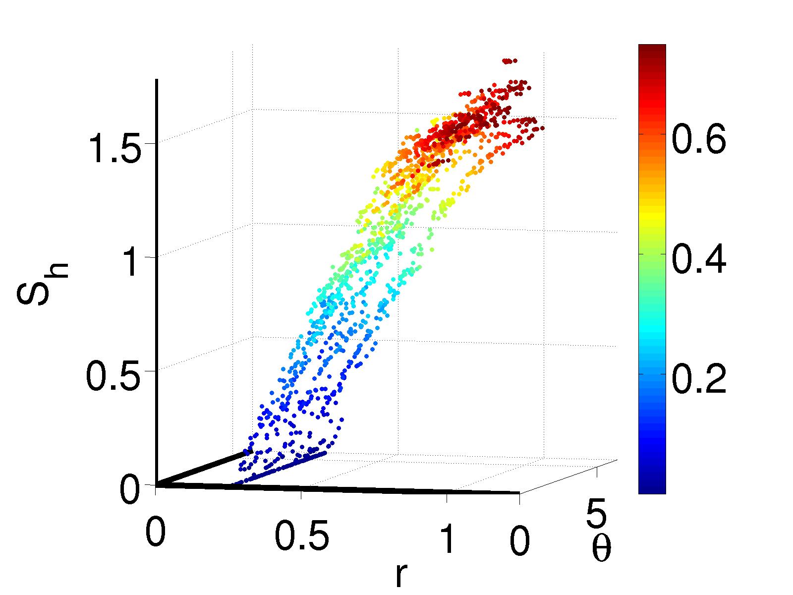
Figure 3.3: Geodesics Estimates $S_{h}(r,\theta)$ on Modified Annulus. Left to Right: $h=1,\ 0.1,\ 0.001$

Fig. 3.3 shows (in the $z$ axis) the estimate $S_{h}(x)$ as $h$ grows small. The colors of the points reflect the true distance to ${\mathcal{A}}$: $S(r)=S_{0}(r)=r-r_{0}$. Note the convergence as $h{\downarrow}0$, and also the clear offset of $S_{h}$ which is especially apparent in the right pane near $r=0.25$.

From the second of Eqs. (3.19) and the fact that $\nabla S(r)=1,\Delta S(r)=1/r$, we have $Z_{0}/r+2Z^{\prime}_{0}=0$ for $r_{0}<r\leq 1$ and $Z_{0}=1$ for $r=r_{0}$. Solving this we get $Z_{0}(r)=\sqrt{r_{0}/r}$. The solution becomes $f_{h}(r)=e^{-(r-r_{0})/h}(\sqrt{r_{0}/r}+O(h))$, which matches the earlier series expansion of the full solution. Furthermore, upon an additional Taylor expansion we have $S_{h}(r)=r-r_{0}-h\log(r_{0}/r)/2+O(h\log h)$. As before, the extra term in the $S_{h}$ estimate has a large effect when $r-r_{0}$ is small (as seen in the right pane of Fig. 3.3).

3.5 Conclusion and Future Work

We have proved that the solution to the SSL problem (3.4) converges to the sampling of a smooth solution of a Regularized Laplacian PDE, in certain limiting cases. Furthermore, we have applied the established theory of Viscosity PDE solutions to analyze this Regularized Laplacian PDE. Our analysis leads to a geometric framework for understanding the regularized graph Laplacian in the noiseless, low regularization regime (where $h\to 0$). This framework provides intuitive explanations for, and validation of, machine learning algorithms that use the inverse of a regularized Laplacian matrix.

We have taken the first steps in extending the theoretical analysis in this chapter to manifolds with boundary (§3.4.3) While the results within this section can be confirmed numerically, in some cases additional work must be done to confirm them in full generality. Furthermore, Assum. 3.3.1 awaits confirmation within the viscosity theory community.

There are a host of applications derived from the work in this chapter, and we turn our focus to them in chapter 4.

Chapter 4 The Inverse Regularized Laplacian: Applications

4.1 Introduction

Thanks to the theoretical development in chapter 3, we now have a framework within which we can construct new tools for learning (e.g. a regularized geodesic distance estimator and a new multiclass classifier). These tools can also shed light on other results in the literature (e.g. a result of [74]). Throughout this chapter we will use the notation developed in chapter 3.

4.2 Regularized Nearest Sub-Manifold (NSM) Classifier

We now construct a new robust geodesic distance estimator and employ it for classification. We then demonstrate the classifier’s efficacy on several standard data sets. To construct the estimator, first choose some anchor set ${\mathcal{A}}\subset{\mathcal{M}}$, and suppose the points $\left\{x_{i}\right\}_{i=1}^{l}$ are sampled from ${\mathcal{A}}$. To calculate the distance $d_{\mathcal{A}}(x_{i})$ for $i=l+1\ldots n$, construct the normalized graph Laplacian ${L_{\epsilon}}$. Choosing $\widetilde{h}>0$ appropriately, solve the linear system (3.7):

$$(E_{\mathcal{A}}+E_{\mathcal{A}^{\prime}}(I+\widetilde{h}^{2}{L_{\epsilon}}))a=\widetilde{w}$$ (4.1)

where $\widetilde{w}=\left[1\ \cdots\ 1\ \ 0\ \cdots\ 0\ \right]^{T}$ is a vector of all zeros for sample points in ${\mathcal{A}^{\prime}}$ and all ones for sample points in ${\mathcal{A}}$. For $n$ large, $\epsilon$ small, and $\widetilde{h}$ small, this linear system approximates (3.9) with $h=\widetilde{h}\sqrt{c}$. Applying Thm. 3.3.10, we see that $\widetilde{S}_{i}=-\widetilde{h}\log a_{i}\approx c^{-1/2}d_{\mathcal{A}}(x_{i})$.

While the estimator $\widetilde{S}$ is approximate and only valid up to a constant, it is also simple to implement and consistent (due to Cor. 3.3.6).

We know of two other consistent geodesics estimators that work on point samples from ${\mathcal{M}}$. One performs fast marching by constructing complex local upwind schemes that require the iterative solution of sequences of high dimensional quadratic systems [88]. Another performs fast marching in ${\mathbb{R}}^{p}$ on offsets of ${\mathcal{X}}$ and is also approximate [71]. The first scheme is complex to implement; the second is exponential in the ambient dimension $p$. Our estimator, on the other hand, can be implemented in Matlab in under 10 lines, given one of many fast approximate NN estimators. Furthermore, it requires the solution of a linear system of size essentially $n$, so its complexity depends only on the number of samples $n$, not on the ambient dimension $p$. Finally, our scheme allows for a natural regularization by tweaking the viscosity parameter $\widetilde{h}$. §4.8 contains numerical comparisons between our estimator and, e.g. Dijkstra’s Shortest Path and Sethian’s Fast Marching estimators.

The lack of dynamic range in the estimator $\widetilde{S}$, following (4.1), leads to important numerical considerations. According to Thm. 3.3.10, for a given sampling ${\mathcal{X}}$ one would choose $\widetilde{h}\ll\min_{e\in{\mathcal{E}}}{\tilde{d}}_{e}$ to have an accurate estimate of geodesics for all point samples. In this case, however, many points far from ${\mathcal{A}}$ may have their associated estimate $a_{i}$ drop below the machine epsilon. In this case an iterative multiscale approach will work: estimates are first calculated for points nearest to ${\mathcal{A}}$ for which no estimate yet exists (but $a_{i}$ is above machine epsilon), then $\widetilde{h}$ is multiplied by some factor $\gamma>1$, and the process is repeated.

We now use the above estimator to form the Nearest Sub-Manifold (NSM) classifier. The classifier is based on two simplifications. First, for noisy samples, one would want to select $\widetilde{h}$ based on the noise level or via cross-validation; it therefore becomes a regularization term. Second, as seen in §3.3.9, for classification the exact estimate of geodesic distance is less important than relative distances; hence there is no need to estimate scaling constants.

As before, suppose we are given $n$ samples from a manifold ${\mathcal{M}}$. Of these, each of the first $l$ belong to one of $M$ classes; that is, $x_{i}\in{\mathcal{C}}_{m}$, $m\in\left\{1,\ldots,M\right\}$. We assume that all points within class $m$ belong to a smooth closed subset of ${\mathcal{M}}$, which we call anchor ${\mathcal{A}}_{m}$, $m=1,\ldots,M$. For each anchor, we define the anchor data vector $\widetilde{w}^{m}$ via $\widetilde{w}^{m}_{i}=\delta(x_{i}\in{\mathcal{C}}_{m})$, $i=1,\ldots,n$. To classify, first choose $\widetilde{h}>0$ and solve (4.1) for each of the $M$ different anchor sets ${\mathcal{A}}_{m}$ (and associated $\widetilde{w}^{m}$), to get solutions $\left\{a^{m}\right\}_{m=1}^{M}$. Then for each unlabeled point $x_{i}$, $a^{m}_{i}$ encodes its distance to anchor ${\mathcal{A}}_{m}$. The decision rule is $C(x_{i})=\operatorname*{argmax}_{m}a^{m}_{i}$.

For $n$ and $l$ large, $\epsilon$, $\widetilde{h}>0$ small, and no noise, $C(x_{i})$ will accurately estimate the class which is closest in geodesic distance to $x_{i}$. In the noisy, finite sample case with irregular boundaries, $C$ provides a regularized estimate of the same.

4.3 NSM Classifier: Performance

We compare the classification performance of the NSM classifier to several state-of-the-art classifiers using the test set from [19] (testing protocol and datasets: http://www.kyb.tuebingen.mpg.de/ssl-book/). For the NSM classifier, we performed a parameter search as described in [19, §21.2.5], and additionally cross-validated over the viscosity parameter $\widetilde{h}\in\left\{0.1,1,10\right\}$ scaled by the median distance between pairs of points in ${\mathcal{E}}$.

We compare our results with publicly available implementations of:

• LapRLS from M. Belkin’s website, with obvious modifications for one-vs-all multiclassification and with the exception that, as opposed to [19], we used $p=1$ in the kernel ${\tilde{L}_{\epsilon}}^{p}$ instead of $p=2$. Here, we also performed a parameter search as in [19, §21.2.5].

• LDS from O. Chapelle’s website with parameters optimized as in [19, §21.2.11].

• Kernel TSVM using primal gradient descent (available in the LDS package) with parameters optimized as in [19, §21.2.1].

For testing, we also included the LIBRAS (LIB) dataset with 12 splits of $l=30,100$ labeled points and the ionosphere (Ion) dataset with 12 splits of $l=10,100$ labeled points. All datasets have $M=2$ (the task is binary classification) except COIL, which has $M=6$.

Table 4.1 shows percent classification error vs. percentage labeled points, over 12 randomized splits of the testing and training data set. Parameter optimization (cross-validation) was always performed on the training splits only; classification error is reported over the testing data. Note that that the NSM classifier is competitive with the others, especially on those datasets where we expect a manifold structure (e.g. the image sets USPS and COIL).

Table 4.1: Percent classification error over 12 splits. Clear winners in bold.

	USPS		BCI		g241n		COIL		LIB		Ion
$100(l/n)$	0.66	6.66	2.5	25	0.66	6.66	0.66	6.66	8.3	28	2.8	28
$l$	10	100	10	100	10	100	10	100	30	100	10	100
NSM	10.0	5.9	49.0	44.8	46.0	39.0	58.8	11.6	51.0	30.3	30.4	14.2
LapRLS	15.0	10.6	48.7	45.4	43.0	33.9	63.1	20.6	48.9	30.4	31.9	13.0
LDS	22.5	11.5	48.7	46.0	49.0	41.0	56.7	16.2	54.9	36.6	17.3	13.5
TSVM	17.4	12.0	48.8	46.1	47.3	23.7	69.5	39.9	66.0	36.6	48.1	20.7

4.4 Irregular Boundaries and the counterexample of Nadler et al.

We relate the Annulus example (Ex. 3.3.1) to a negative result of [74, Thm. 2], which essentially states that no solution exists for (3.9) for ${\mathcal{M}}$ with $d\geq 2$ and the anchor set a countable number of points. This yields a special case of a result known in PDE theory: no solution exists to (3.9) when ${\mathcal{A}}$ is irregular; and isolated points on subsets of ${\mathbb{R}}^{d}$, $d\geq 2$, are irregular [47, Irregular Boundary Point].

This is very clearly seen in Ex. 3.3.1, where attempting to let $r_{0}\to 0$ (thus forcing a single point anchor) forces the first term of the solution $f_{h}$ in (3.24) to zero for any $r>r_{0}$, regardless of the anchor condition at $r=r_{0}$ and of $h$. The major culprit here is the $(d-1)/r$ term that appears in the radial Laplacian and is unbounded at the origin. Note, however, that viscosity solutions to (3.10) do exist even for singular anchors [68].

In many practical cases (i.e., if we had chosen single point anchors in §3.3.9, Ex. 3.3.2, etc), the sampling size is finite and we keep $\epsilon\geq\epsilon_{0}$ for some $\epsilon_{0}>0$. In these cases, the issues raised here do not affect the numerical analysis because even single points act like balls of radius $\epsilon$ in ${\mathbb{R}}^{p}$.

4.5 Beyond Classification: Graph Denoising, Manifold Learning

The ideas presented in the previous sections can also be applied to other areas of machine learning. As illustrations, we show that the graph denoising scheme of [13] is a special case of our geodesics estimator. Further, we show how to construct a regularized variant of ISOMAP and provide some numerical examples of geodesics estimation.

4.6 The Graph Denoising Algorithm of Chapter 2

In chapter 2, we studied decision rules for denoising (removing) edges from NN graphs that have been corrupted by sampling noise. We examine the Neighborhood Probability Decision Rule (NPDR) of §2.4, and show that in the low noise, low regularization regime, it removes graph edges between geodesically distant points.

The NPDR is constructed in three stages: (a) the NN graph $G$ is constructed from the sample points ${\mathcal{X}}$. ${\mathcal{E}}$ contains an initial estimate of neighbors in $G$, but may contain incorrect edges due to sampling noise; (b) a special Markov random walk is constructed on $G$, resulting in the transition probability matrix ${N_{\epsilon}}\propto(I-{\bar{p}}{P_{\epsilon}})^{-1}$ for ${\bar{p}}\in(0,1)$; (c) the edges $(l,k)=e\in{\mathcal{E}}$ with the smallest associated entries $({N_{\epsilon}})_{lk}$ are removed from $G$. In chapter 2, we provide a probabilistic interpretation for the coefficients of ${N_{\epsilon}}$.

We show that ${N_{\epsilon}}$ encodes geodesic distances by reducing ${N_{\epsilon}}^{-1}$ to look like (3.9):

$$I-{\bar{p}}{P_{\epsilon}} =(1-{\bar{p}})I+{\bar{p}}(I-{P_{\epsilon}})\propto({1}/{\epsilon})I+{{\bar{p}}}(1-{\bar{p}})^{-1}{L_{\epsilon}}.$$ (4.2)

For $\epsilon$ small, after applying the RHS of (4.2), ${N_{\epsilon}}e_{i}$ approximately solves (3.9) with ${\mathcal{A}}=\left\{x_{i}\right\}$, $w(x_{i})=c^{\prime}$ (where $c^{\prime}$ is a function of ${{\bar{p}},\epsilon}$), and $h^{2}=c\epsilon{\bar{p}}/(1-{\bar{p}})$. Then by Thm. 3.3.10

$$({N_{\epsilon}})_{lk}\approx c^{\prime}e^{-d(x_{l},x_{k})\sqrt{(1-{\bar{p}})/(c\epsilon{\bar{p}})}},\mbox{some }c^{\prime}>0.$$

Thus in the noiseless case and with ${\bar{p}}\approx 0$, the NPDR algorithm will remove edges in the graph between points that are geodesically far from each other. As edges of this type are the most detrimental to learning [3], the NPDR is a powerful denoising rule. As shown in chapter 2, for noisy samples one would choose ${\bar{p}}\approx 1$ to regularize for noisy edges. In this case, one can think of ${N_{\epsilon}}$ as a highly regularized encoding of pairwise geodesic distances.

4.7 Viscous ISOMAP

As a second example of how the ideas from §3.3.9 can be used, we construct a regularized variant of ISOMAP [105], which we call Viscous ISOMAP.

ISOMAP is a dimensionality reduction algorithm that constructs an embedding for $n$ points sampled from a high-dimensional space by performing Multidimensional Scaling (MDS) on the estimated geodesic distance matrix of the NN graph of these points.

The first step of ISOMAP is to estimate all pairwise geodesic distances. Traditionally this is done via Dijkstra’s Shortest Path algorithm. We replace this step with our regularized geodesics estimator. A direct implementation requires $n$ calculations of (4.1). However, a faster estimator can be constructed, based on our analysis of the NPDR algorithm in §4.6. Specifically, to calculate pairwise distances, first calculate $M=(I+\widetilde{h}^{2}{L_{\epsilon}})^{-1}$. Then the symmetrized geodesics estimates are $H=-\widetilde{h}(\log M+\log M^{T})$, where the logarithm is taken elementwise. Finally, perform MDS on the matrix $H$ to calculate the ISOMAP embedding.

For small $\widetilde{h}$, the Viscous ISOMAP embedding matches that of standard ISOMAP. For large $\widetilde{h}$, the additional regularization can remove the effects of erroneous edges caused by noise and outliers.

We provide a rather simple numerical example. It confirms that for small viscosity $\widetilde{h}$, Viscous ISOMAP embeddings match standard ISOMAP embeddings, and that for larger viscosities the embeddings are less sensitive to outliers in the original sampling set ${\mathcal{X}}$ and in ${\mathcal{E}}$.

Fig. 4.1 compares Viscous ISOMAP to regular ISOMAP on a noisy Swiss Roll with topological shortcuts. We used the same $n=1000$ samples and $\delta=4$ for NN estimation for both algorithms, and $\epsilon=1$ for Viscous ISOMAP. Note how for small $\widetilde{h}$, the Viscous ISOMAP embedding matches the standard one. Also note how increasing the viscosity term $\widetilde{h}$ leads to the an accurate embedding in the principal direction, “unrolling” the Swiss Roll.

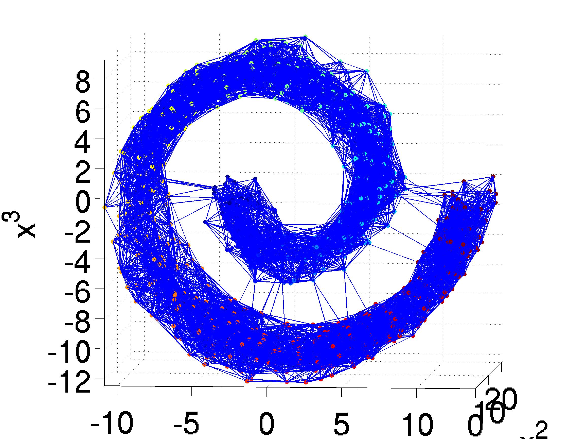
Figure 4.1: ISOMAP vs. Viscous ISOMAP. Top Left: Noisy Swiss Roll, Top Right: ISOMAP Embedding, first 2 components. Bottom Left: Viscous ISOMAP Embedding, $\widetilde{h}=.1$. Bottom Right: Viscous ISOMAP Embedding, $\widetilde{h}=20$.

4.8 Numerical Examples of Geodesics Estimation

We provide two examples of Geodesic Estimation: on the Torus, and on a triangulated mesh. For the Torus, we used the normalized Graph Laplacian of §3.3.1 and ground truth geodesic distances were given by Dijkstra’s Shortest Path algorithm. On the mesh, we used the mesh surface Laplacian of [7], and for ground truth geodesic distances the mesh Fast Marching algorithm of [57] (As implemented in Toolbox Fast Marching at http://www.ceremade.dauphine.fr/~peyre/). In both cases, $S_{h}$ was calculated via the geodesics estimator of §4.2; thus, as always, $S_{h}$ estimates geodesic distances up to a constant.

Example 4.8.1 (The Torus $T=S^{1}{\times}S^{1}$ in ${\mathbb{R}}^{3}$).

The torus $T$ is defined by the points $(x^{1},x^{2},x^{3})=((2+\cos v^{1})\cos v^{2},(2+\cos v^{1})\sin v^{2},\sin v^{2})$ for $v^{1}\in[0,2\pi)$ and $v^{2}\in[0,2\pi)$. We used $n=1000$ randomly sampled points, with $k=100$ neighbors for the initial NN graph, $\epsilon=.01$ and $\widetilde{h}=.001$. Setting ${\mathcal{A}}=\left\{x_{i}\right\}$, $i=1,3$ where $x_{1}$ corresponds to $(v^{1},v^{2})=(0,0)$, and $x_{3}$ is a randomly chosen point, we can calculate geodesic distances of all points in ${\mathcal{X}}$ to these anchors. The results are shown in Fig. 4.2.

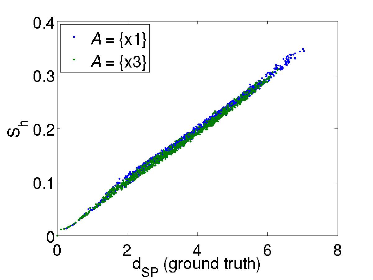
Figure 4.2: Geodesics Estimation on $T$. Top Left: $S_{h}(x)$ in ${\mathbb{R}}^{3}$; ${\mathcal{A}}=\left\{x_{1}\right\}$. Top Right: $S_{h}(v^{1},v^{2})$ in the parameter space; ${\mathcal{A}}=\left\{x_{1}\right\}$. Bottom: $S_{h}$ vs. Shortest Path estimates for ${\mathcal{A}}=\left\{x_{1}\right\}$, $\left\{x_{3}\right\}$.

Example 4.8.2 (The Dancing Children Mesh).

The Dancing Children mesh is a complex (high genus) mesh from the Aim$@$Shape Repository (http://shapes.aimatshape.net/). The mesh $G$ is composed of $n\approx 36000$ vertices; and we used $\epsilon=.1$ (times the mean edge distance), and $\widetilde{h}=.01$ for the estimation procedure. The anchor point $x_{1}$ was chosen randomly. Our results are shown in Fig. 4.3. Note that minor discrepancies between the Fast Marching estimate $d_{FM}$ and our estimate $S_{h}$ occur near areas with complex topology and areas of high curvature (e.g. near a hole in the mesh).

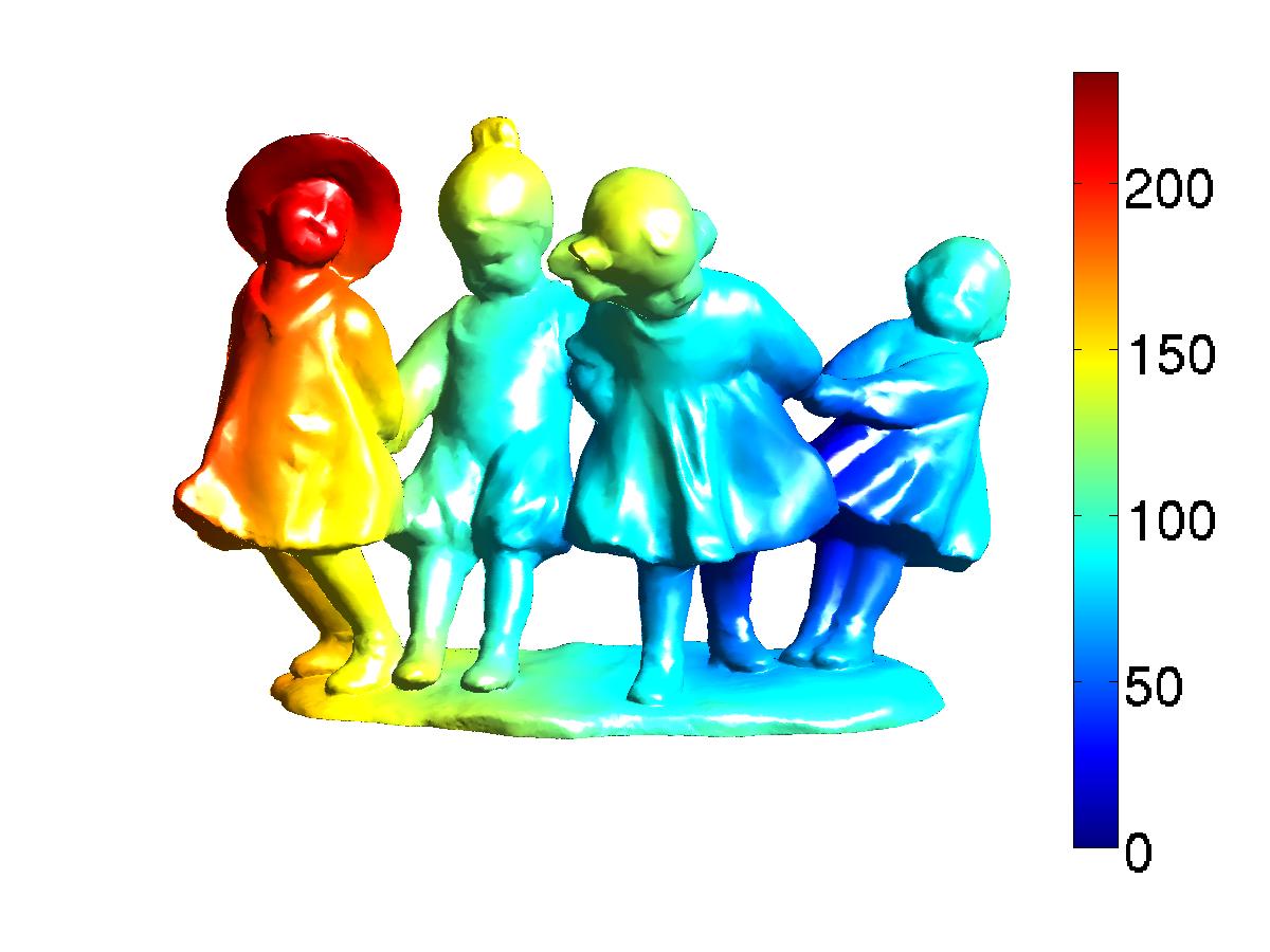
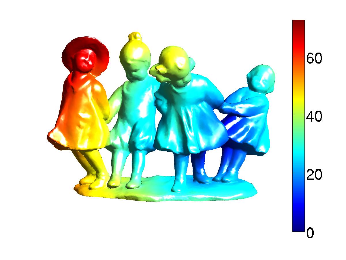
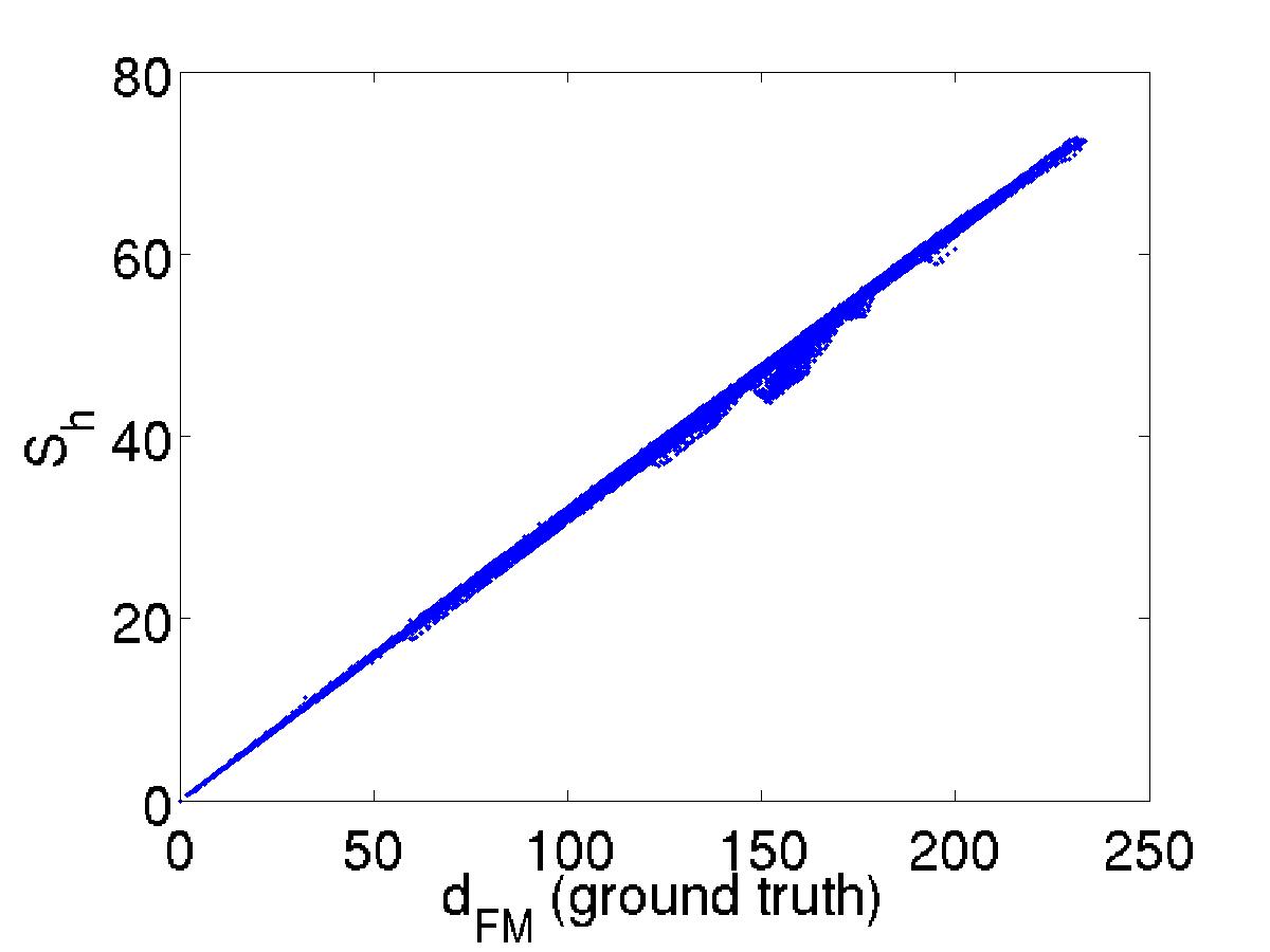
Figure 4.3: Geodesics Estimation on the Dancing Children mesh. Top Left: Fast Marching Estimate $d_{FM}(x)$ on the mesh; ${\mathcal{A}}=\left\{x_{1}\right\}$. Top Right: $S_{h}(x)$ on the mesh; ${\mathcal{A}}=\left\{x_{1}\right\}$. Bottom: $S_{h}$ vs. Fast Marching estimates for ${\mathcal{A}}=\left\{x_{1}\right\}$.

Chapter 5 Synchrosqueezing

5.1 Introduction

In this chapter, we analyze the Synchrosqueezing transform, a consistent and invertible time-frequency analysis tool that can identify and extract oscillating components (of time-varying frequency and amplitude) from regularly sampled time series. We first describe a fast algorithm implementing the transform. Second, we show Synchrosqueezing is robust to bounded perturbations of the signal. This stability property extends the applicability of Synchrosqueezing to the analysis of nonuniformly sampled and noisy time series, which are ubiquitous in engineering and the natural sciences. Numerical simulations show that Synchrosqueezing provides a natural way to analyze and filter a variety of signals. In Chapter 6, we use Synchrosqueezing to analyze a variety of data, including ECG signals and climate proxies.

The purpose of this chapter is twofold. We first describe the Synchrosqueezing transform in detail and highlight the subtleties of a new fast numerical implementation. Second, we show both numerically and theoretically that Synchrosqueezing is stable under bounded signal perturbations. It is therefore robust to noise and to errors incurred by preprocessing using approximations, such as interpolation.

The chapter is organized as follows. We first describing Synchrosqueezing, and in §5.4 we provide a fast new implementation. In §5.5 we provide theoretical evidence that Synchrosqueezing analysis and reconstruction are stable to bounded perturbations. In §5.6, we numerically compare Synchrosqueezing to other common transforms, and provide examples of its stability properties. Conclusions and ideas for future theoretical work are in §5.8.

Comprehensive numerical examples and applications are deferred to Chapter 6.

5.2 Prior Work

Synchrosqueezing is a tool designed to extract and compare oscillatory components of signals that arise in complex systems. It provides a powerful method for analyzing signals with time-varying behavior and can give insight into the structure of their constituent components. Such signals $f(t)$ have the general form

$$f(t)\,=\,\sum_{k=1}^{K}f_{k}(t)+e(t),$$ (5.1)

where each component $f_{k}(t)=A_{k}(t)\cos(\phi_{k}(t))$ is an oscillating function, possibly with smoothly time-varying amplitude and frequency, and $e(t)$ represents noise or observation error. The goal is to extract the amplitude factor $A_{k}(t)$ and the Instantaneous Frequency (IF) $\phi^{\prime}_{k}(t)$ for each $k$.

Signals of the form (5.1) arise naturally in engineering and scientific applications, where it is often important to understand their spectral properties. Many time-frequency (TF) transforms exist for analyzing such signals, such as the Short Time Fourier Transform (STFT), Wavelet Transform, and Wigner-Ville distribution [40], but these methods can fail to capture key short-range characteristics of the signals. As we will see, Synchrosqueezing deals well with such complex data.

Synchrosqueezing is a TF transform that is ostensibly similar to the family of time-frequency reassignment (TFR) algorithms, methods used in the estimation of IFs in signals of the form given in (5.1). TFR analysis originates from a study of the STFT, which smears the energy of the superimposed IFs around their center frequencies in the spectrogram. TFR analysis “reassigns” these energies to sharpen the spectrogram [41, 42]. However, there are some significant differences between Synchrosqueezing and most standard TFR techniques.

Synchrosqueezing was originally introduced in the context of audio signal analysis [32]. In [31], it was further analyzed theoretically as an alternative way to understand the Empirical Mode Decomposition (EMD) algorithm [50]. EMD has proved to be a useful tool for analyzing and decomposing natural signals. Like EMD, Synchrosqueezing can extract and clearly delineate components with time varying spectrum. Furthermore, like EMD, and unlike most TFR techniques, it allows individual reconstruction of these components.

5.3 Synchrosqueezing: Analysis

Synchrosqueezing is performed in three steps. First, the Continuous Wavelet Transform (CWT) $W_{f}(a,b)$ of $f(t)$ is calculated [29]. Second, an initial estimate of the FM-demodulated frequency, $\omega_{f}(a,b)$, is calculated on the support of $W_{f}$. Finally, this estimate is used to squeeze $W_{f}$ via reassignment; we thus get the Synchrosqueezing representation $T_{f}(\omega,b)$. Synchrosqueezing is invertible: we can calculate $f$ from $T_{f}$. Our ability to extract individual components stems from filtering $f$ by keeping energies from specific regions of the support of $T_{f}$ during reconstruction.

Note that Synchrosqueezing, as originally proposed [32], estimates the FM-demodulated frequency from the wavelet representation $W_{f}(a,b)$ before performing reassignment. However, it can be adapted to work on “on top of” many invertible transforms (e.g. the STFT [106]). We focus on the original wavelet version as described in [31].

We now detail each step of Synchrosqueezing, using the harmonic signal $h(t)=A\cos(\Omega t)$ for motivation. As a visual aid, Fig. 5.1 shows each step on the signal $h(t)$ with $A=1$ and $\Omega=4\pi$. Note that Figs. 5.1(b,d) show that Synchrosqueezing is more “precise” than the CWT.

Figure 5.1: Synchrosqueezing example for $h(t)=\cos(4\pi t)$. Clockwise: a) $h(t)$, sampled, $n=1024$ points. b) CWT of $h$, $|W_{h}|$. c) FM-demodulated frequency from $W_{h}$, ${\omega}_{h}$. d) Synchrosqueezing of $h$: $|T_{h}|$; line at $w_{\hat{l}}\approx 2$.

5.3.1 CWT of ${f(t)}$

For a given mother wavelet $\psi$, the CWT of $f$ is given by $W_{f}(a,b)=\int_{-\infty}^{\infty}f(t)a^{-1/2}\overline{\psi\left(\frac{t-b}{a}\right)}dt,$ where $a$ is the scale and $b$ is the time offset. We assume that $\psi$ has fast decay, and that its Fourier transform $\widehat{\psi}(\xi)=(2\pi)^{-1/2}\int_{-\infty}^{\infty}\psi(t)e^{-i\xi t}dt$ is approximately zero in the negative frequencies : $\widehat{\psi}(\xi)\approx 0$ for $\xi<0$, and is concentrated around some positive frequency $\xi=\omega_{0}$ [31]. Many wavelets have these properties (several examples and compared in §5.7). For $h(t)$, the harmonic signal above, upon applying our assumptions we get $W_{h}(a,b)=\frac{1}{2\sqrt{2\pi}}Aa^{1/2}\overline{\widehat{\psi}(a\Omega)}e^{ib\Omega}$.

5.3.2 Calculate the FM-demodulated frequency ${\omega(a,b)}$

The wavelet representation of the harmonic signal $h(t)$ (with frequency $\Omega$) will have its energy spread out in the time-scale plane around the line $a=\omega_{0}/\Omega$, and this frequency will be encoded in the phase [32, 31]. In those regions where $\left\lvert W_{h}\right\rvert>0$ we would like to remove the effect of the Wavelet on this frequency. We perform a type of FM demodulation by taking derivatives: $(W_{h}(a,b))^{-1}\partial_{b}W_{h}(a,b)=i\Omega$. This simple model leads to an estimate of the frequency in the time-scale plane:

$$\omega_{f}(a,b)=\begin{cases}\frac{-i\partial_{b}W_{f}(a,b)}{W_{f}(a,b)}&|W_{f}(a,b)|>0\\ \infty&|W_{f}(a,b)|=0\end{cases}.$$ (5.2)

5.3.3 Squeezing in the time-frequency plane: ${T_{f}(\omega,b)}$

The final step of Synchrosqueezing is reassigning energy in the time-scale plane to the TF plane according to the frequency map $(a,b)\to(\omega(a,b),b)$. Reassignment follows from the inversion property of the CWT: when $f(t)$ is real,

$$f(b)=2{\mathcal{R}}_{\psi}^{-1}\operatorname{\mathfrak{Re}}{\left(\int_{0}^{\infty}W_{f}(a,b)a^{-3/2}da\right)},$$ (5.3)

where ${\mathcal{R}}_{\psi}=\sqrt{2\pi}\int_{0}^{\infty}\xi^{-1}\overline{\widehat{\psi}(\xi)}d\xi$ is a normalizing constant.

We first break up the integrand in (5.3) according to the FM-demodulated frequency estimate $\omega_{f}$. Define frequency divisions $\left\{w_{l}\right\}_{l=0}^{\infty}$ s.t. $w_{0}>0$ and $w_{l+1}>w_{l}$ for all $l$. Further, let the frequency bin ${\mathcal{W}}_{l}$ be the set of points $w^{\prime}\in{\mathbb{C}}$ closer to $w_{l}$ than to any other $w_{l}^{\prime}$. We define the Discrete-Frequency Wavelet Synchrosqueezing transform of $f$ as:

$$T_{f}(w_{l},b)=\int_{\left\{a:\omega_{f}(a,b)\in{\mathcal{W}}_{l}\right\}}W_{f}(a,b)a^{-3/2}da.$$ (5.4)

In other words, $T_{f}(w_{l},b)$ is the “volume” of the frequency preimage set ${\mathcal{W}}_{l}^{-1}(b)=\left\{a:\omega_{f}(a,b)\in{\mathcal{W}}_{l}\right\}$ under the signed measure $\mu_{f,b}(a)=W_{f}(a,b)a^{-3/2}da$.

This definition has several favorable properties. First, it allows us to reconstruct $f$ from $T_{f}$:

$$f(b)=2{\mathcal{R}}_{\psi}^{-1}\operatorname{\mathfrak{Re}}{\left(\sum_{l}T_{f}(w_{l},b)\right)}.$$ (5.5)

Second, for the harmonic signal $h(t)$, with $\omega_{h}(a,b)=\Omega$, there will be a single $\hat{l}$ such that $w_{\hat{l}}$ is closest to $\omega_{h}(a,b)$. From (5.3), we have $h(b)=2\operatorname{\mathfrak{Re}}{\left({\mathcal{R}}_{\psi}^{-1}T_{h}(w_{\hat{l}},b)\right)}$. Further, the magnitude of $T_{h}$ is proportional to that of $h(t)$: $\left\lvert T_{h}(w_{\hat{l}},b)\right\rvert=\frac{\left\lvert A\right\rvert}{2\pi}\left\lvert{\mathcal{R}}_{\psi}\right\rvert$.

More generally, for a wide class of signals with slowly varying $A_{k}(t)$ and well separated ${\phi_{k}^{\prime}}(t)$, given a sufficiently fine division of the frequency bins $\left\{w_{l}\right\}$, each of the $K$ components can be well concentrated into its own “curve” in the TF plane (see Thm. 5.5.1 below). This allows us to analyze such signals: by looking at $\left\lvert T_{f}(w,b)\right\rvert$ to identify and extract the curves, and to reconstruct their associated components.

5.4 A Fast Implementation

In practice, we observe the vector ${\tilde{f}}\in{\mathbb{R}}^{n}$, $n=2^{L+1}$, where $L$ is a nonnegative integer. Its elements, ${\tilde{f}}_{m},m=0,\ldots,n-1$, correspond to a uniform discretization of $f(t)$ taken at the time points $t_{m}=t_{0}+m\Delta t$. To prevent boundary effects, we pad ${\tilde{f}}$ on both sides (using, e.g., reflecting boundary conditions).

We now describe a fast numerical implementation of Synchrosqueezing. The speed of our algorithm lies in two key steps. First, we calculate the Discrete Wavelet Transform (DWT) of the vector ${\tilde{f}}$ using the Fast Fourier Transform (FFT). Second, we discretize the squeezing operator $T$ in a way that lends itself to a fast numerical implementation.

5.4.1 DWT of sampled signal ${\tilde{f}}$

The DWT samples the CWT $W_{f}$ at the locations $(a_{j},t_{m})$, where $a_{j}=2^{j/n_{v}}\Delta t$, $j=1,\ldots,Ln_{v}$, and the number of voices $n_{v}$ is a user-defined “voice number” parameter [43] (we have found that $n_{v}=32$ works well). The DWT of ${\tilde{f}}$ can be calculated in $O(n_{v}n\log_{2}^{2}n)$ operations using the FFT. We outline the steps below.

First note that $W_{f}(a,b)=\left[a^{-1/2}\overline{\psi(-t/a)}*f(t)\right](b)$, where $*$ denotes convolution over $t$. In the frequency domain, this relationship becomes: $\widehat{W}_{f}(a,\xi)=a^{1/2}\widehat{f}(\xi)\widehat{\psi}(a\xi)$. We use this to calculate the DWT, ${\widetilde{W}}_{\tilde{f}}(a_{j},t_{m})$. Let ${\mathcal{F}}_{n}$ (${\mathcal{F}}_{n}^{-1}$) be the standard (inverse) circular Discrete Fourier Transform. Then

$${\widetilde{W}}_{\tilde{f}}(a_{j},\cdot)={\mathcal{F}}_{n}^{-1}\left(({\mathcal{F}}_{n}{\tilde{f}})\odot\widehat{\psi}_{j}\right).$$ (5.6)

Here $\odot$ denotes elementwise multiplication and $\widehat{\psi}_{j}$ is an $n$-length vector with $(\widehat{\psi}_{j})_{m}=a_{j}^{1/2}\widehat{\psi}(a_{j}\xi_{m})$; $\xi_{m}$ are samples in the unit frequency interval: $\xi_{m}=2\pi m/n$, $m=0,\ldots,n-1$.

5.4.2 A Stable Estimate of $\omega_{f}$: $\widetilde{\omega}_{\tilde{f}}$

We first require a slight modification of the FM-demodulated frequency estimate (5.2),

$$\omega_{f}(a,b)=\operatorname{\mathfrak{Im}}{\left((W_{f}(a,b))^{-1}\partial_{b}W_{f}(a,b)\right)}.$$ (5.7)

This definition is equivalent to (5.2) when Synchrosqueezing is performed via (5.4), and simplifies the algorithm.

In practice, signals have noise and other artifacts due to, e.g., sampling errors, and the phase of $W_{f}$ is unstable when $\left\lvert W_{f}\right\rvert\approx 0$. As such the user should choose some $\gamma>0$ (we often use $\gamma\approx 10^{-8}$) as a hard threshold on $\left\lvert W_{f}\right\rvert$. We define the numerical support of ${\widetilde{W}}_{\tilde{f}}$, on which $\omega_{f}$ can be estimated:

$\widetilde{{\mathcal{S}}}^{\gamma}_{\tilde{f}}(m)=\left\{j:\left\lvert{\widetilde{W}}_{\tilde{f}}(a_{j},t_{m})\right\rvert>\gamma\right\}$, for $m=0,\ldots,n-1$.

The estimate of $\omega_{f}$, $\widetilde{\omega}_{\tilde{f}}$, can be calculated by taking differences of ${\widetilde{W}}_{\tilde{f}}$ with respect to $m$ before applying (5.7), but we provide a more direct way. Let Using the property $\widehat{\partial_{b}W_{f}}(a,\xi)=i\xi\widehat{W_{f}}(a,\xi)$, we estimate the FM-demodulated frequency, for $j\in\widetilde{{\mathcal{S}}}^{\gamma}_{\tilde{f}}(m)$, as

$\widetilde{\omega}_{\tilde{f}}(a_{j},t_{m})=\operatorname{\mathfrak{Im}}{\left(\left({\widetilde{W}}_{\tilde{f}}(a_{j},t_{m})\right)^{-1}\partial_{b}{\widetilde{W}}_{\tilde{f}}(a_{j},t_{m})\right)},$

with the time derivative of $W_{f}$ estimated via (e.g., [104]):

$\partial_{b}{\widetilde{W}}_{\tilde{f}}(a_{j},\cdot)={\mathcal{F}}^{-1}_{n}\left(({\mathcal{F}}_{n}{\tilde{f}})\odot\widehat{\partial\psi}_{j}\right),$

where $(\widehat{\partial\psi}_{j})_{m}=a_{j}^{1/2}i\xi_{m}\widehat{\psi}(a_{j}\xi_{m})/\Delta t$ for $m=0,\ldots,n-1$.

Finally, we normalize $\widetilde{\omega}$ by $2\pi$ so that the dominant frequency estimate is $\alpha$ when $f(t)=\cos(2\pi\alpha t)$.

5.4.3 Fast estimation of ${T_{f}}$ from ${{\widetilde{W}}_{\tilde{f}}}$ and ${\widetilde{\omega}_{\tilde{f}}}$

The representation ${\widetilde{W}}_{\tilde{f}}$ is given with respect to $n_{a}=Ln_{v}$ log-scale samples of the scale $a$, and this leads to several important considerations when estimating $T_{f}$ via (5.3) and (5.4). First, due to lower resolutions in coarser scales, we expect to get lower resolutions in the lower frequencies. We thus divide the frequency domain into $n_{a}$ components on a log scale. Second, sums with respect to $a$ on a log scale, $a(z)=2^{z/n_{v}}$ with $da(z)=a\frac{\log 2}{n_{v}}dz$, lead to the modified integrand ${W_{f}(a,b)a^{-1/2}\frac{\log 2}{n_{v}}dz}$ in (5.4).

To choose the frequency divisions, note that the discretization period $\Delta t$ limits the maximum frequency $\overline{w}$ that can be estimated. The Nyquist theorem suggests that this frequency is $\overline{w}=w_{n_{a}-1}=\frac{1}{2\Delta t}$. Further, if we assume periodicity, the maximum period of an input signal is $n\Delta t$; thus the minimum frequency is $\underline{w}=w_{0}=\frac{1}{n\Delta t}$. Combining these limits with the log scaling of the $w$’s we get the divisions: $w_{l}=2^{l\Delta w}\underline{w}$, $l=0,\ldots,n_{a}-1$, where $\Delta w=\frac{1}{n_{a}-1}\log_{2}(n/2)$. Note, the voice number $n_{v}$ has a big effect on the frequency resolution.

We can now calculate the Synchrosqueezed estimate ${\widetilde{T}}_{\tilde{f}}$. Our fast implementation of (5.4) finds the associated ${\mathcal{W}}_{l}$ for each $(a_{j},t_{m})$ and adds it to the correct sum, instead of performing a search over all scales for each $l$. This is possible because $\widetilde{\omega}_{\tilde{f}}(a_{j},t_{m})$ only ever lands in one frequency bin. We provide pseudocode for this $O(n_{a})$ implementation in Alg. 1.

Algorithm 1 Fast calculation of ${\widetilde{T}}_{\tilde{f}}$ for fixed $m$

  for $l=0$ to $n_{a}-1$ do {Initialize ${\widetilde{T}}$ for this $m$}

     ${\widetilde{T}}_{{\tilde{f}}}(w_{l},t_{m})\leftarrow 0$

  end for

  for all $j\in\widetilde{{\mathcal{S}}}^{\gamma}_{{\tilde{f}}}(m)$ do {Calculate (5.4)}

     {Find frequency bin via $w_{l}=2^{l\Delta w}\underline{w}$, and $\widetilde{\omega}_{{\tilde{f}}}\in{\mathcal{W}}_{l}$}

     $l\leftarrow\textrm{ROUND}\left[\frac{1}{\Delta w}\log_{2}\left(\frac{\widetilde{\omega}_{{\tilde{f}}}(a_{j},b_{m})}{\underline{w}}\right)\right]$

     if $l\in[0,n_{a}-1]$ then

        {Add normalized term to appropriate integral; $\Delta z=1$}

        ${\widetilde{T}}_{{\tilde{f}}}(w_{l},t_{m})\leftarrow{\widetilde{T}}_{{\tilde{f}}}(w_{l},t_{m})+\frac{\log 2}{n_{v}}{\widetilde{W}}_{{\tilde{f}}}(a_{j},t_{m})a^{-1/2}_{j}$

     end if

  end for

5.4.4 IF Curve Extraction and Filtered Reconstruction

A variety of signals, especially sums of quasi-harmonic signals with well-separated IFs, will have a frequency image $\left\lvert T_{f}(w,b)\right\rvert$ composed of several curves in the $(w,b)$ plane. The image of the $k$th curve corresponds to both the IF ${\phi_{k}^{\prime}}(b)$, and the entire component $A_{k}(b)\cos(\phi_{k}(b))$.

To extract a discretized curve $c^{*}$ we maximize a functional of the energy of the curve that penalizes variation:

$$\max_{c\in\left\{w_{l}\right\}^{n}}\sum_{m=0}^{n-1}E_{\tilde{f}}(w_{c_{m}},t_{m})-\lambda\sum_{m=1}^{n-1}\Delta w|c_{m}-c_{m-1}|^{2},$$ (5.8)

where $E_{\tilde{f}}(w_{l},t_{m})=\log(|{\widetilde{T}}_{\tilde{f}}(w_{l},t_{m})|^{2})$ is the normalized energy of ${\widetilde{T}}$. The user-defined parameter $\lambda>0$ determines the “smoothness” of the resulting curve estimate (we use $\lambda=10^{5}$). Its associated component ${\tilde{f}}^{*}$ can be reconstructed via (5.5), by restricting the sum over $l$, at each $t_{m}$, to the neighborhood ${\mathcal{N}}_{m}=[{c^{*}_{m}-n_{w}},{c^{*}_{m}+n_{w}}]$ (we use the window size $n_{w}=n_{v}/2$). The next curve is extracted by setting ${\widetilde{T}}_{\tilde{f}}({\mathcal{N}}_{m},t_{m})=0$ for all $m$ and repeating the process above.

5.5 Consistency and Stability of Synchrosqueezing

We first review the main theorem on wavelet-based Synchrosqueezing, as developed in [31] (Thm. 5.5.1). Then we show that the components extracted via Synchrosqueezing are stable to bounded perturbations such as noise and discretization error.

We specify a class of functions on which these results hold. In practice, Synchrosqueezing works on a wider function class.

Definition 5.5.1 (Sums of Intrinsic Mode Type (IMT) Functions).

The space $\mathcal{A}_{\epsilon,d}$ of superpositions of IMT functions, with smoothness $\epsilon$ and separation $d$, consists of functions having the form $f(t)=\sum_{k=1}^{K}f_{k}(t)$ with $f_{k}(t)=A_{k}(t)e^{i\phi_{k}(t)}$. For $t\in{\mathbb{R}}$ the IF components $\phi^{\prime}_{k}$ are ordered and relatively well separated (high frequency components are spaced further apart than low frequency ones):

$$\forall t\quad\phi_{k}^{\prime}(t) >\phi_{k-1}^{\prime}(t),\quad\text{and}$$

$$\inf_{t}\phi^{\prime}_{k}(t)-\sup_{t}\phi^{\prime}_{k-1}(t) \geq d(\inf_{t}\phi^{\prime}_{k}(t)+\sup_{t}\phi^{\prime}_{k-1}(t)).$$

Functions in the class $\mathcal{A}_{\epsilon,d}$ are essentially composed of components with time-varying amplitudes. Furthermore, the amplitudes vary slowly, and the individual IFs are sufficiently smooth. For each $k$,

$$A_{k}\in L^{\infty}\cap C^{1},\quad\phi_{k}\in C^{2},\quad\phi^{\prime}_{k},\phi^{\prime\prime}_{k}\in L^{\infty},\quad\phi^{\prime}_{k}(t)>0,$$

$$\|A^{\prime}_{k}\|_{L^{\infty}}\leq\epsilon\|\phi^{\prime}_{k}\|_{L^{\infty}},\quad\text{and}\quad\|\phi^{\prime\prime}_{k}\|_{L^{\infty}}\leq\epsilon\|\phi^{\prime}_{k}\|_{L^{\infty}}.$$

For the theoretical analysis, we also define the Continuous Wavelet Synchrosqueezing transform, a smooth version of $T_{f}$.

Definition 5.5.2 (Continuous Wavelet Synchrosqueezing).

Let $h\in C_{0}^{\infty}$ be a smooth function such that $\left\lVert h\right\rVert_{L^{1}}=1$. The Continuous Wavelet Synchrosqueezing transform of function $f$, with accuracy $\delta$ and thresholds $\epsilon$ and $M$, is defined by

$$S_{f,\epsilon}^{\delta,M}(b,\eta)=\int_{\Gamma_{f,\epsilon}^{\delta,M}}\frac{W_{f}(a,b)}{a^{3/2}}\delta^{-1}h\left(\frac{\left\lvert\eta-\omega_{f}(a,b)\right\rvert}{\delta}\right)da$$ (5.9)

where $\Gamma_{f,\epsilon}^{M}=\left\{(a,b):a\in[M^{-1},M],|W_{f}(a,b)|>\epsilon\right\}$. We also denote $S_{f,\epsilon}^{\delta}=S_{f,\epsilon}^{\delta,\infty}$ and $\Gamma_{f,\epsilon}^{\infty}=\Gamma_{f,\epsilon}$, where the condition $a\in[M^{-1},M]$ is replaced by $a>0$.

The continuous ($S_{f}^{\delta}$) and discrete frequency ($T_{f}$) Synchrosqueezing transforms are equivalent for small $\delta$ and large $n_{v}$, respectively. The frequency term $\eta$ in (5.9) is equivalent to $w_{l}$ in (5.4), and the integrand term $\frac{1}{\delta}h(\frac{\cdot}{\delta})$ in (5.9) takes the place of constraining the frequencies to ${\mathcal{W}}_{l}$ in (5.4). Signal reconstruction and filtering analogues via the continuous Synchrosqueezing transform thus reduce to integrating $S_{f,\epsilon}^{\delta}$ over $\eta>0$, similar to summing over $l$ in (5.5).

The following consistency theorem was proved in [31]:

Theorem 5.5.1 (Synchrosqueezing Consistency).

Suppose $f\in{\mathcal{A}}_{\epsilon,d}$. Pick a wavelet $\psi\in C^{1}$ such that its Fourier transform $\widehat{\psi}(\xi)$ is supported in $[1-\Delta,1+\Delta]$ for some $\Delta<\frac{d}{1+d}$. Then for sufficiently small $\epsilon$, Synchrosqueezing can identify and extract the components $\left\{f_{k}\right\}$ from $f$:

1. The Synchrosqueezing plot $|S^{\delta}_{f}|$ is concentrated around the IF curves $\{\phi_{k}^{\prime}\}$. For each $k$, define the “scale band” $Z_{k}=\{(a,b):|a\phi_{k}^{\prime}(b)-1|<\Delta\}$. For sufficiently small $\epsilon$, the FM-demodulated frequency estimate $\omega_{f}$ is accurate inside $Z_{k}$ where $W_{f}$ is sufficiently large ($|W_{f}(a,b)|>{\epsilon^{1/3}}$):

$\left\lvert\omega_{f}(a,b)-\phi_{k}^{\prime}(b)\right\rvert\leq{\epsilon^{1/3}}$.

Outside the scale bands $\left\{Z_{k}\right\}$, $W_{f}$ is small:

$|W_{f}(a,b)|\leq{\epsilon^{1/3}}$.

2. Each component $f_{k}$ may be reconstructed by integrating $S^{\delta}_{f}$ over a neighborhood around $\phi_{k}^{\prime}$. Choose the Wavelet threshold $\epsilon^{1/3}$ and let $N_{k}(b)=\{\eta:|\eta-\phi^{\prime}_{k}(b)|\leq{\epsilon^{1/3}}\}$. For sufficiently small $\epsilon$, there is a constant $C_{1}$ such that for all $b\in\mathbb{R}$,

$$\left|\lim\limits_{\delta\rightarrow 0}\left(\mathcal{R}_{\psi}^{-1}\int_{N_{k}(b)}S_{f,\epsilon^{1/3}}^{\delta}(b,\eta)d\eta\right)-f_{k}(b)\right|\leq C_{1}\epsilon^{1/3}.$$

Note that, as expected, Thm. 5.5.1 implies that components $f_{k}$ with low amplitude may be difficult to identify and extract (as their Wavelet magnitudes may fall below $\epsilon^{1/3}$).

Thm. 5.5.1 also applies to discrete Synchrosqueezing, with the following modifications: letting $\delta\to 0$ is equivalent to letting $n_{v}\to\infty$. For reconstruction via (5.5), the integral over $\eta$ should be replaced by a sum over $l$ in the discrete neighborhood $N_{k}(b)=\left\{l:\left\lvert w_{l}-\phi^{\prime}_{k}(b)\right\rvert\leq\epsilon^{1/3}\right\}$. Finally, the threshold $\epsilon^{1/3}$ in Thm. 5.5.1 part 2 can be applied numerically by letting $\gamma>\epsilon^{1/3}$ when calculating the discrete support ${\mathcal{S}}_{{\tilde{f}}}^{\gamma}$.

We prove the following theorem in [12]:

Theorem 5.5.2 (Synchrosqueezing stability to small perturbations).

The statements in Thm. 5.5.1 essentially still hold if $f$ is corrupted by a small error $e$, especially for mid-range IFs.

Let $f\in\mathcal{A}_{\epsilon,d}$ and suppose we have a corresponding $\epsilon$, $h$, $\psi$, $\Delta$, and $Z_{k}$ as given in Thm. 5.5.1. Furthermore, assume that $g=f+e$, where $e$ is a bounded perturbation such that $\left\lVert e\right\rVert_{L^{\infty}}\leq C_{\psi}\epsilon$, where $C_{\psi}^{-1}=\max(\|\psi\|_{L^{1}},\|\psi^{\prime}\|_{L^{1}})$. For each $k$ define the “maximal frequency range” $M_{k}\geq 1$ such that $\phi^{\prime}_{k}(t)\in[M^{-1},M]$ for all $t$. A mid-range IF is defined as having $M_{k}$ near $1$.

1. The Synchrosqueezing plot $|S_{g}^{\delta}|$ is concentrated around the IF curves $\left\{\phi_{k}^{\prime}\right\}$. For sufficiently small $\epsilon$, the FM-demodulated frequency estimate $\omega_{g}$ is accurate inside $Z_{k}$ where $W_{g}$ is sufficiently large ($|W_{g}(a,b)|>M_{k}^{1/2}\epsilon+{\epsilon^{1/3}}$):

$|\omega_{g}(a,b)-\phi_{k}^{\prime}(b)|\leq C_{2}\epsilon^{1/3}$,

where $C_{2}=O(M_{k})$. Outside the scale bands $\left\{Z_{k}\right\}$, $W_{g}$ is small:

$|W_{g}(a,b)|\leq M_{k}^{1/2}\epsilon+{\epsilon^{1/3}}$.

2. Each component $f_{k}$ may be reconstructed with accuracy proportional to the noise magnitude and its maximal frequency range by integrating $S_{g}^{\delta}$ over a neighborhood around $\phi_{k}^{\prime}$. Choose the wavelet threshold $M_{k}^{1/2}{\epsilon^{1/3}}+\epsilon$ and let $N^{\prime}_{k}(b)=\left\{\eta:|\eta-\phi^{\prime}_{k}(b)|\leq C_{2}\epsilon^{1/3}\right\}$, where (as before) $C_{2}=O(M_{k})$. For sufficiently small $\epsilon$,

$$\left|\lim_{\delta\rightarrow 0}\left(\mathcal{R}_{\psi}^{-1}\int\limits_{N^{\prime}_{k}(b)}S_{g,M_{k}^{1/2}\epsilon+\epsilon^{1/3}}^{\delta,M_{k}}(b,\eta)d\eta\right)-f_{k}(b)\right|\leq C_{3}\epsilon^{1/3},$$

where $C_{3}=O(M_{k})$.

Thm. 5.5.2 has two important implications. First, components with mid-range IF tend to have the best estimates and lowest reconstruction error under bounded noise. Second, to best identify signal component $f_{k}$ with IF $\phi^{\prime}_{k}\in[M^{-1},M]$, from a noisy signal, the threshold $\gamma$ should be chosen proportional to $M^{1/2}\epsilon$, where $\epsilon$ is an estimate of the noise magnitude.

5.5.1 Stability under Spline Interpolation

In many applications, samples of a signal $f\in{\mathcal{A}}$ are only given at irregular sample points $\left\{t^{\prime}_{m}\right\}$, and these are spline interpolated to a function $f_{s}$. Thm. 5.5.2 bounds the error incurred due to this preprocessing:

Corollary 5.5.3.

Let $\displaystyle D=\max_{m}|t^{\prime}_{m+1}-t^{\prime}_{m}|$ and let $e=f_{s}-f$. Then the error in the estimate of the $k$th IF of $T_{f_{s}}$ is $O(M_{k}D^{4/3})$, and the error in extracting $f_{k}$ is $O(M_{k}D^{4/3})$.

Proof.

This follows from Thm. 5.5.2 and the following standard estimate on cubic spline approximations [102, p. 97]:

$\left\|e\right\|_{L^{\infty}}\leq\frac{5}{384}D^{4}\|f^{(4)}\|_{L^{\infty}}.$

∎

Thus, we can Synchrosqueeze $f_{s}$ instead of $f$ and, as long as the minimum sampling rate $D^{-1}$ is high enough, the results will match. Furthermore, in practice errors are localized in time to areas of low sampling rate, low component amplitude, and/or high component frequency (see, e.g., §5.6).

5.6 Examples of Synchrosqueezing Properties

We now provide numerical examples of several important properties of Synchrosqueezing. First, we compare Synchrosqueezing with two common analysis transforms.

5.6.1 Comparison of Synchrosqueezing to the CWT and STFT

We compare Synchrosqueezing to the Wavelet transform and the Short Time Fourier Transform (STFT) [77]. We show its superior precision, in both time and frequency, at identifying components of sums of quasi-harmonic signals.

Figure 5.2: Comparison of Synchrosqueezing with Wavelet and the STFT. (a) Synthetic signal $s(t)$. (b) Short Time Fourier Transformed signal. (c) Wavelet transformed: $W_{s}(a,t)$. (d) Synchrosqueezed: $T_{s}(\omega,t)$.

In Fig. 5.2 we focus on a signal $s(t)$ defined on $t\in[0,10]$, that contains an abrupt transition at $t=5$, and time-varying AM and FM modulation. It is discretized to $n=1024$ points and is composed of the following components:

$$t<5:s_{1}(t) =.5\cos(2\pi(3t)),s_{2}(t)=.5\cos(2\pi(4t)),$$

$$s_{3}(t) =.5\cos(2\pi(5t))$$

$$t\geq 5:s_{1}(t) =\cos(2\pi(.5t^{1.5})),$$

$$s_{2}(t) =\exp(-t/20)\cos(2\pi(.75t^{1.5})),$$

$$s_{3}(t) =\cos(2\pi t^{1.5}).$$

We used the shifted bump wavelet (see §5.7) and $n_{v}=32$ for both the Wavelet and Synchrosqueezing transforms, and a Hamming window with length 300 and overlap of length 285 for the STFT. These STFT parameters focused on optimal precision in frequency, but not in time [77]. For $t<5$, the harmonic components of $s(t)$ are clearly identified in the Synchrosqueezing plot $T_{s}$ (Fig. 5.2(d)) and the STFT plot (Fig. 5.2(b)), though the frequency estimate is more precise in $T_{s}$. The higher frequency components are better estimated up to the singularity at $t=5$ in $T_{s}$, but in the STFT there is mixing at the singularity. For $t\geq 5$, the frequency components are more clearly visible in $T_{s}$ due to the smearing of lower frequencies in the STFT. The temporal resolution in the STFT is also significantly lower than for Synchrosqueezing due to the selected parameters. A shorter window in the STFT will provide higher temporal resolution, but lower frequency resolution and more smearing between the three components.

5.6.2 Nonuniform Sampling and Splines

We now demonstrate how Synchrosqueezing and extraction work for a more complicated signal that contains multiple time-varying amplitude and frequency components, and has been irregularly subsampled. Let

$$f(t) =\cos(4\pi t)$$ (5.10)

$$+(1+0.2\cos(2.5t))\cos(2\pi(5t+2t^{1.2}))$$

$$+e^{-0.2t}\cos(2\pi(3t+0.2\cos(t))),$$

and let the sampling times be perturbations of uniformly spaced times having the form $t^{\prime}_{m}=\Delta t_{1}m+\Delta t_{2}u_{m}$, where $\Delta t_{2}<\Delta t_{1}$ and $\{u_{m}\}$ is sampled from the uniform distribution on $[0,1]$. Here we fix $\Delta t_{1}=11/180$ and $\Delta t_{2}=11/600$. This leads to $\approx 160$ samples on the interval $t\in[0,10]$. To correct for nonuniform sampling, we fit a spline through $(t^{\prime}_{m},f(t^{\prime}_{m}))$ to get the function $f_{s}(t)$ and discretize on the finer grid $t_{m}=m\Delta t$, with $\Delta t=10/1024$ and $m=0,\ldots,1023$. The resulting vector, ${\tilde{f}}_{s}$, is a discretization of the original signal plus a spline error term. Fig. 5.3(a) shows ${\tilde{f}}_{s}$ for $t\in[2,8]$.

Figure 5.3: (a) Nonuniform Sampling of $f$, with spline interpolation estimate ${\tilde{f}}_{s}$. (b) Synchrosqueezing $\widetilde{T}_{{\tilde{f}}_{s}}$ of ${\tilde{f}}_{s}$; components extracted via (5.8). (c-e) Extracted components ${\tilde{f}}^{*}_{k}$ compared to originals ${\tilde{f}}_{k}$, $k=1,2,3$ (respectively).

Figs. 5.3(b-e) show the results of Synchrosqueezing and component extraction of ${\tilde{f}}_{s}$, for $t\in[2,8]$. All three components are well separated in the TF domain. The second component is the most difficult to reconstruct, as it contains the highest frequency information. Due to stability (Thm. 5.5.2 and Cor. 5.5.3), extraction of components with mid-range IFs is more stable to the error $e(t)$. Fig. 5.3 shows that reconstruction errors are time localized to the locations of errors in ${\tilde{f}}_{s}$.

5.6.3 White Noise and Reconstruction

We take the signal $f(t)$ of (5.10), now regularly sampled on the fine grid with $\Delta t=10/1024$ ($n=1024$ samples) as before, and corrupt it with white Gaussian noise having a standard deviation of $\sigma_{N}=1.33$. This signal, ${\tilde{f}}_{N}$ (see Fig. 5.4(a)) has an SNR of $-1$ dB.

Figure 5.4: (a) Uniform sampling of $f$, ${\tilde{f}}$, corrupted by normal white noise with standard deviation $\sigma_{N}=1.33$ (SNR is $-1$ dB): ${\tilde{f}}_{N}$. (b) Synchrosqueezing $\widetilde{T}_{{\tilde{f}}_{N}}$ of ${\tilde{f}}_{N}$; components extracted via (5.8). (c-e) Extracted components ${\tilde{f}}^{*}_{k}$ compared to originals ${\tilde{f}}_{k}$, $k=1,2,3$ (respectively).

Figs. 5.4(b-e) show the results of Synchrosqueezing and component extraction of ${\tilde{f}}_{N}$, for $t\in[2,8]$. As seen in Fig. 5.4(b), most of the additional energy, caused by the white noise, appears in the higher frequencies. Again, all three components are well separated in the TF domain, though now the third, lower-amplitude, component experiences a “split” at $t\approx 6.5$. Reconstruction of signal components is less reliable in locations of high frequencies and low magnitudes (note the axis in Fig. 5.4(e) is half that of the others). This again numerically confirms Thm. 5.5.2: components with mid-range IFs and higher amplitudes are more stable to the noise.

5.7 Invariance to the underlying transform

As mentioned in §5.3 and in [31], Synchrosqueezing is invariant to the underlying choice of transform. The only differences one sees in practice are due to two factors: the time compactness of the underlying analysis atom (e.g. mother wavelet), and the frequency compactness of this atom. That is, $\left\lvert\psi(t)\right\rvert$ should fall off quickly away from zero, $\widehat{\psi}(\xi)$ is ideally zero for $\xi<0$, and $\Delta$ (of Thm. 5.5.1) is small.

Fig. 5.5 shows the effect of Synchrosqueezing the discretized spline signal ${\tilde{f}}_{s}$ of the synthetic nonuniform sampling example in §5.6.2, using three different complex CWT mother wavelets. These wavelets are:

a. Morlet (shifted Gaussian)

$$\qquad\widehat{\psi}_{a}(\xi)\propto\exp(-(\mu-\xi)^{2}/2),\quad\xi\in{\mathbb{R}}$$

b. Complex Mexican Hat

$$\qquad\widehat{\psi}_{b}(\xi)\propto\xi^{2}\exp(-\sigma^{2}\xi^{2}/2),\quad\xi>0$$

c. Shifted Bump

$$\qquad\widehat{\psi}_{d}(\xi)\propto\exp\left(-(1-((\xi-\mu)/\sigma)^{2})^{-1}\right),$$

$$\qquad\xi\in[\sigma(\mu-1),\sigma(\mu+1)]$$

where for $\psi_{a}$ we use $\mu=2\pi$, for $\psi_{b}$ we use $\sigma=1$, for and for $\psi_{c}$ we use $\mu=5$ and $\sigma=1$.

Figure 5.5: Wavelet and Synchrosqueezing transforms of ${\tilde{f}}_{s}$. Columns (a-c) represent choice of mother wavelet $\psi_{a}\ldots\psi_{c}$. Top row: $|2\widehat{\psi}(4\xi)|$. Center row: $|W_{f_{s}}|$. Bottom row: $|T_{f_{s}}|$.

The Wavelet representations of ${\tilde{f}}_{s}$ differ due to differing mother wavelets, but the Synchrosqueezing representation is mostly invariant to these differences. As expected from Thm. 5.5.1, more accurate representations are given by wavelets having compact frequency support on $\xi$ away from $0$.

5.8 Conclusions and Future Work

Synchrosqueezing can be used to extract the instantaneous spectra of, and filter, a wide variety of signals that include complex simulation data (e.g. dynamical models), and physical signals (e.g. climate proxies). A careful implementation runs in $O(n_{v}n\log^{2}n)$ time, and is stable (in theory and in practice) to errors in these types of signals.

Areas in which Synchrosqueezing has shown itself to be an important analysis tool include ECG analysis (respiration and T-end detection), meteorology and oceanography (large-scale teleconnection and ocean-atmosphere interaction), and climatology. Some of these examples are described in the next chapter.

Additional future work includes theoretical analysis of the Synchrosqueezing transform, including the development of Synchrosqueezing algorithms that directly support nonuniform sampling, the analysis of Synchrosqueezing when the signal is perturbed by Gaussian, as opposed to bounded, noise, and extensions to higher dimensional data.

Chapter 6 Synchrosqueezing: Applications

6.1 Introduction

The theoretical results of Chapter 5 provide important guarantees and guidelines for the use of Synchrosqueezing in data analysis techniques. Here, we focus on two specific applications in which Synchrosqueezing, in combination with preprocessing methods such as spline interpolation, provides powerful new analysis tools.

This chapter is broken down into two sections. First, we use Synchrosqueezing and spline interpolation to estimate patients’ respiration from the R-peaks (beats) in their Electrocardiogram (ECG) signals. This extends earlier work on the ECG-Derived Respiration problem.

Second, we visit open problems in paleoclimate studies of the last 2.5 Myr, where Synchrosqueezing provides improved insights. We compare a calculated solar flux index with a deposited $\delta^{18}O$ paleoclimate proxy over this period. Synchrosqueezing cleanly delineates the orbital cycles of the solar radiation, provides an interpretable representation of the orbital signals of $\delta^{18}O$, and improves our understanding of the effect that the solar flux distribution has had on the global climate. Compared to previous analyses of these data, the Synchrosqueezing representation provides more robust and precise estimates in the time-frequency plane.

6.2 ECG Analysis: Respiration Estimation

We first demonstrate how Synchrosqueezing can be combined with nonuniform subsampling of a single lead ECG recording to estimate the instantaneous frequency of, and in some cases extract, a patients’s respiration signal. We verify the accuracy of our estimates by comparing them with the instantaneous frequency (IF) extracted from a simultaneously recorded respiration signal.

The respiratory signal is usually recorded mechanically via, e.g., spirometry or plethysmography. There are two common disadvantages to these techniques. First, they require the use of complicated devices that might interfere with natural breathing. Second, they are not appropriate in many situations, such as ambulatory monitoring. However, having the respiratory signal is often important, e.g. for the diagnosis of obstructive sleep apnea. Thus, finding a convenient way to directly record, or indirectly estimate, information about the respiration signal is important from a clinical perspective.

ECG is a cheap, non-invasive, and ubiquitous technique, in which voltage differences are passively measured between electrodes (leads) connected to a patient’s body (usually the chest and arms). The change of the thoracic electrical impedance caused by inhalation and exhalation, and thus physiological respiratory information, is reflected in the ECG amplitude. The respiration-induced distortion of ECG was first studied in [36] and [39]. A well-known ECG-Derived Respiration (EDR) technique [73] experimentally showed that “electrical rotation” during the respiratory cycle is the main contributor to the distortion of ECG amplitude, and that the contribution of thoracic impedance variations is relatively minor. These prior work confirm that analyzing ECG may enable us to estimate respiration. More details about EDR are available in [66].

Relying on the coupling between physiological respiration and R-peak amplitudes (the tall spikes in Fig. 6.1(a)), we use the R-peaks as a proxy for the respiration signal. More specifically, we hypothesize that the R peaks, taken as samples of the envelope of the ECG signal $f_{E}(t)$, have the same IF profile as the true respiration signal $f_{R}(t)$. By sampling $f_{E}(t)$ at the R peaks and performing spline interpolation on the resulting samples, we hope to see a time shifted, amplitude scaled, version of $f_{R}(t)$ near the respiratory frequency (0.25Hz).

Figure 6.1: (a) ECG signal and spline R-peak envelope; $t\in[120,180]$. (b) Respiration, full (black), filtered (green), and estimated from ECG R-peak envelope (red).

Figure 6.2: (a) Synchrosqueezing of ECG spline R-peak envelope ${\tilde{f}}_{EP}$ with main extracted curve representing ${\tilde{f}}_{EP_{1}}$; $t\in[0,600]$ and $\omega\in[.2\pi,2\pi]$. (b) Synchrosqueezing of Respiration ${\tilde{f}}_{R}$ with main extracted curve representing ${\tilde{f}}_{R_{1}}$.

In Fig. 6.1, we show the lead II ECG signal and the true respiration signal (via respiration belt) of a healthy $30$ year old male, recorded over a $10$ minute interval ($t\in[0,600]$ sec). The sampling rates of the ECG and respiration signals are respectively 400Hz and 50Hz within this interval. There are $846$ R peaks appearing at nonuniform times $t^{\prime}_{m}\in[0,600]$, $m=1,\ldots,846$. We run cubic spline interpolation on the R-peaks $\{(t^{\prime}_{m},f_{E}(t^{\prime}_{m}))\}$ to get $f_{EP}(t)$, which we discretize at 50Hz (with $n=30000$) to get ${\tilde{f}}_{EP}$. Fig. 6.2 shows the result of running Synchrosqueezing on ${\tilde{f}}_{R}$ and ${\tilde{f}}_{EP}$. The computed IF, ${\tilde{f}}_{EP_{1}}$, turns out to be a good (shifted and scaled) approximation to the IF of the true respiration, ${\tilde{f}}_{R_{1}}$. It can be seen, from Figs. 6.1 and 6.2, that the spacing of respiration cycles in $f_{R}(t)$ is reflected by the main IF of ${\tilde{f}}_{EP}$: closer spacing corresponds to higher IF values, and wider spacing to lower values.

These results were confirmed by tests on several subjects. Thanks to the stability of Synchrosqueezing (Thm. 5.5.2 and Cor. 5.5.3), this algorithm has the potential for broader clinical usage.

6.2.1 Notes on Data Collection and Analysis Parameters

The ECG signal ${\tilde{f}}_{E}$ was collected at 400Hz via a MSI MyECG E3-80. The respiration signal ${\tilde{f}}_{R}$ was collected at 50Hz via a respiration belt and PASCO SW750. The ECG signal was filtered to remove the worst nonstationary noise by thresholding signal values below the $0.01\%$ and above the $99.99\%$ quantiles, to these quantile values. The ECG R-peaks were then extracted from ${\tilde{f}}_{E}$ by first running the physionet ecpguwave  program, followed by a “maximum” peak search within a 0.2 sec window of each of the ecgpuwave-estimated R-peaks.

For Synchrosqueezing, the parameters $\gamma=10^{-8}$ and $\lambda=10^{5}$ were used for thresholding $W_{f}$ and extracting contours from both the R-peak spline and respiratory signals.

6.3 Paleoclimatology: Aspects of the mid-Pleistocene transition

Next, we apply Synchrosqueezing to analyze the characteristics of a calculated index of the incoming solar radiation (insolation) and to measurements of repeated transitions between glacial (cold) and interglacial (warm) climates during the Pleistocene epoch: $\approx$ 1.8 Myr to 12 kyr before the present.

The Earth’s climate is a complex, multi-component nonlinear, system with significant stochastic elements [79]. The key external forcing field is the insolation at the top of the atmosphere (TOA). Local insolation has predominately harmonic characteristics in time (diurnal cycle, annual cycle and Milanković orbital cycles). However, response of planetary climate, which varies at all time scales [52], also depends on random perturbations (e.g., volcanism), solid boundary conditions (e.g., plate tectonics and global ice distribution), internal variability and feedbacks (e.g., global carbon cycle). Various paleoclimate records or proxies provide us with information about past climates beyond observational records. Proxies are biogeochemical tracers, i.e., molecular or isotopic properties, imprinted into various types of deposits (e.g., deep-sea sediment), and they indirectly represent physical conditions (e.g., temperature) at the time of deposition. We focus on climate variability during the last 2.5 Myr (that also includes the late Pliocene) as recorded by ${\delta}^{18}O$ in foraminiferal shells at the bottom of the ocean (benthic forams). Benthic $\delta^{18}O$ is the deviation of the ratio of ${}^{18}O$ to ${}^{16}O$ in sea water with respect to the present-day standard, as imprinted in benthic forams during their growth. It increases with glaciation during cold climates because ${}^{16}O$ evaporates more readily and accumulates in ice sheets. Thus, benthic ${\delta}^{18}O$ can be interpreted as a proxy for either high-latitude temperature or global ice volume.

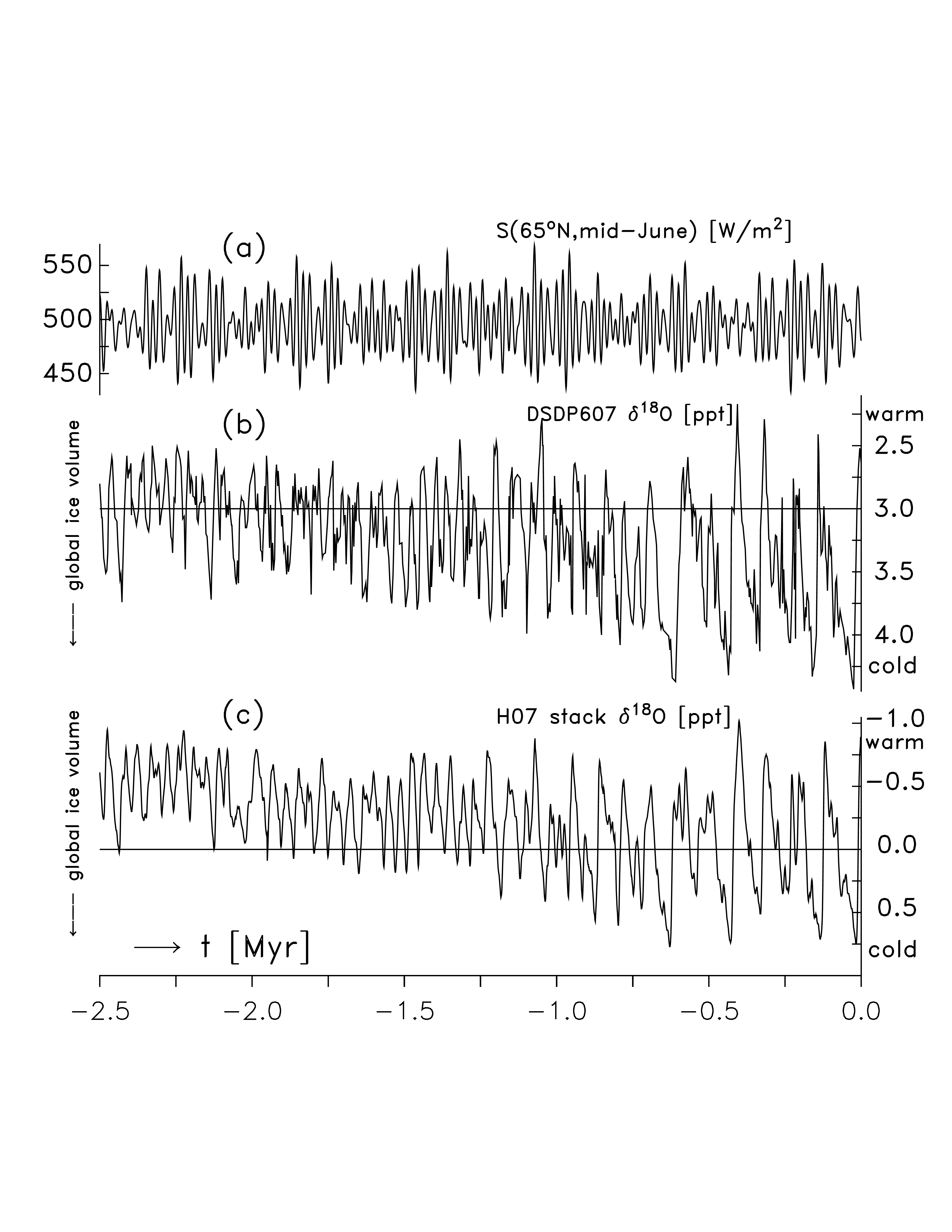
Figure 6.3: (a) Calculated mid-June insolation flux at $65^{o}N$: $f_{SF}$. Climate response as recorded by benthic ${\delta}^{18}O$ (b) in DSDP607 core: $f_{CR1}$, and (c) in H07 stack: $f_{CR2}$.

We first examine a calculated element of the TOA solar forcing field. Fig. 6.3(a) shows $f_{SF}$, the mid-June insolation at $65^{o}N$ at 1 kyr intervals [9]. This TOA forcing index does not encompass the full complexity of solar radiation structure and variability, but is commonly used to gain insight into the timing of advances and retreats of ice sheets in the Northern Hemisphere in this period (e.g., [46]). The Wavelet and Synchrosqueezing decompositions in Fig. 6.4(a) and Fig. 6.5(a), respectively, show the key harmonic components of $f_{SF}$. The application of a shifted bump mother wavelet (see §5.7) yields an upward shift of the spectral features along the scale axis in each of the the representations in Fig. 6.4. Therefore the scale $a$ should not be used to directly infer periodicities. In contrast, the Synchrosqueezing spectrums in Fig. 6.5 explicitly present time-frequency (or here specifically time-periodicity) decompositions with a sharper structure, and are not affected by the scale shift inherent in the choice of mother wavelet.

Fig. 6.5(a) clearly shows the presence of strong precession cycles (at periodicities $\tau$=19 kyr and 23 kyr), obliquity cycles (primary at 41 kyr and secondary at 54 kyr), and very weak eccentricity cycles (primary periodicities at 95 kyr and 124 kyr, and secondary at 400 kyr). This is in contrast with Fig. 6.4(a), which contains blurred and shifted spectral structures only qualitatively similar to Fig. 6.5(a).

We next analyze the climate response during the last 2.5 Myr as deposited in benthic ${\delta}^{18}O$ in long sediments cores. (in which deeper layers contain forams settled further back in time). Fig. 6.3(b) shows $f_{CR1}$: benthic ${\delta}^{18}O$, sampled at irregular time intervals from a single core, DSDP Site 607, in the North Atlantic [84]. This signal was spline interpolated to 1 kyr intervals prior to the spectral analyses. Fig. 6.3(c) shows $f_{CR2}$: the benthic ${\delta}^{18}O$ stack (H07) calculated at 1 kyr intervals from fourteen cores (most of them from the Northern Hemisphere, including DSDP607) using the extended depth-derived age model [51]. Prior to combining the cores in the H07 stack, the record mean between 0.7 Myr ago and the present was subtracted from each ${\delta}^{18}O$ record; this is the cause of the differing vertical ranges in Figs. 6.3(b-c). Noise due to local climate characteristics and measurement errors of each core is reduced when we shift the spectral analysis from DSDP607 to the stack; and this is particularly visible in the finer scales and higher frequencies.

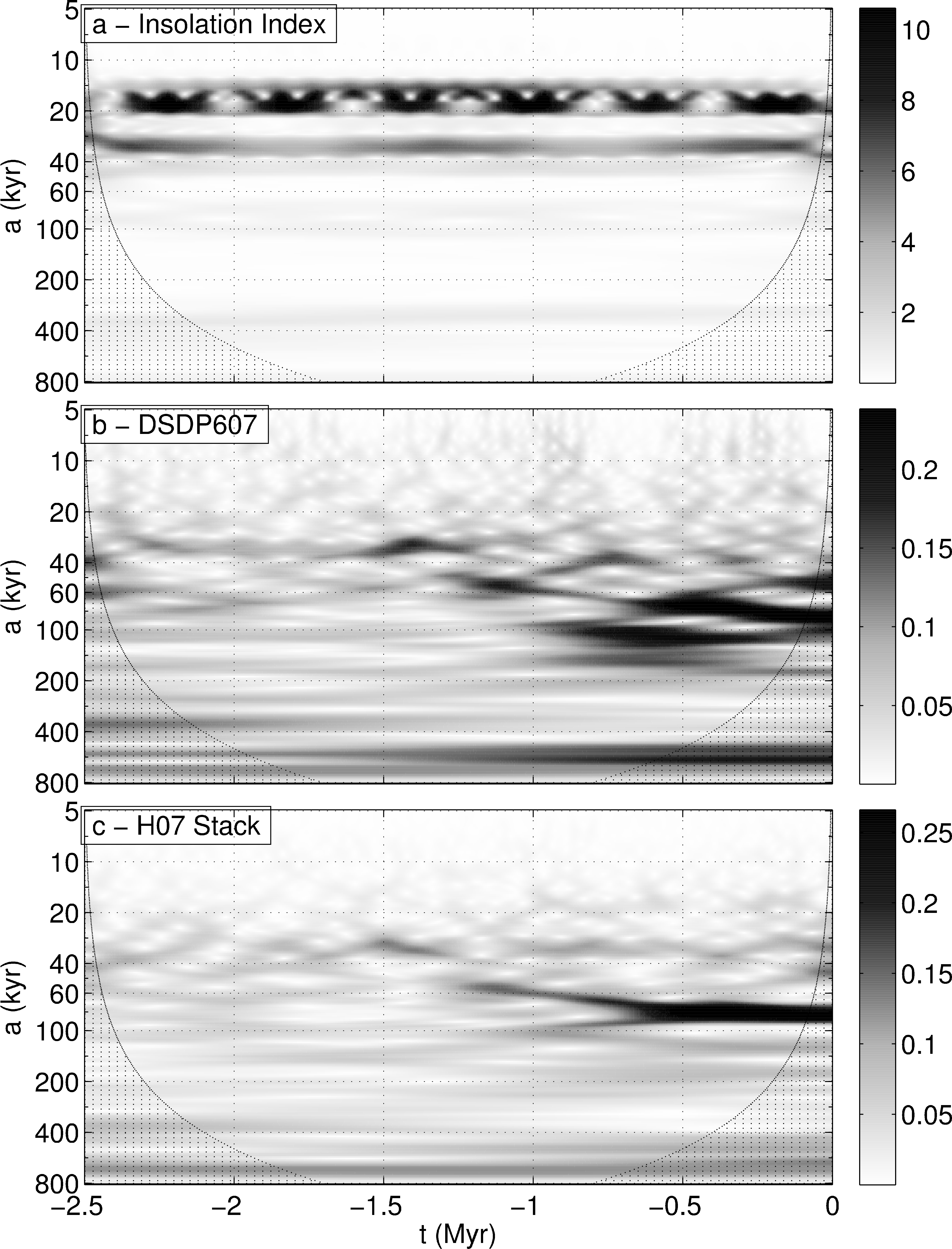
Figure 6.4: Wavelet magnitude time evolution of (a) insolation index $f_{SF}$, and climate response in benthic ${\delta}^{18}O$ of (b) DSDP607 core, $f_{CR1}$, and (c) H07 stack, $f_{CR2}$.

Figure 6.5: Explicit time-periodicity decomposition of Synchrosqueezing spectral magnitude of (a) solar forcing index $f_{SF}$, and climate response in benthic ${\delta}^{18}O$ of (b) DSDP607 core, $f_{CR1}$, and (c) H07 stack, $f_{CR2}$.

The Synchrosqueezing decomposition in Fig. 6.5(c) is a more precise time-frequency representation of the stack than a careful STFT analysis [51, Fig. 4]. In addition, it shows far less stochasticity above the obliquity band as compared to Fig. 6.5(b), enabling the 23 kyr precession cycle to become mostly coherent over the last 1 Myr. Thanks to the stability of Synchrosqueezing, the spectral differences below the obliquity band are less pronounced between Fig. 6.5(b) and Fig. 6.5(c). Overall, the stack reveals sharper time-periodicity evolution of the climate system than DSDP607 or any other single core possibly could. The Wavelet representations in Figs. 6.4(b-c) also show this suppression of noise in the stack (in more diffuse and scale shifted patterns). Figs. 6.6(a) through 6.6(c) show that the time average of Synchrosqueezing magnitudes (normalized by $1/R_{\psi}$) is directly comparable with the Fourier spectrum, but delineates the harmonic components much more clearly (not shown).

During the last 2.5 Myr, the Earth experienced a gradual decrease in global background temperature and $\text{CO}_{2}$ concentration, and an increase in mean global ice volume accompanied with glacial-interglacial oscillations that have intensified towards the present (this is evident in Fig. 6.3(b) and 6.3(c)). The mid-Pleistocene transition, occurring gradually or abruptly sometimes between 1.2 Myr and 0.6 Myr ago, was the shift from 41 kyr-dominated glacial cycles to 100 kyr-dominated glacial cycles recorded in deep-sea proxies (e.g., [85, 22, 80]). The origin of this strong 100 kyr cycle in the late-Pleistocene climate and the prior incoherency of the precession band are still unresolved questions. Both types of spectral analyses of selected ${\delta}^{18}O$ records indicate that the climate system does not respond linearly to external periodic forcing.

Synchrosqueezing enables the detailed time-frequency decomposition of a noisy, nonstationary, climate time series due to stability (Thm. 5.5.2) and more precisely reveals key modulated signals that rise above the stochastic background. The gain (the ratio of the climate response amplitude to insolation forcing amplitude) at a given frequency or period, is not constant. The response to the 41 kyr obliquity cycle is present almost throughout the entire Pleistocene in Fig. 6.5(c). The temporary incoherency of the 41 kyr component starting about 1.25 Myr ago roughly coincides with the initiation of a lower frequency signal ($\approx$ 70 kyr) that evolves into a strong 100 kyr component in the late Pleistocene (about 0.6 Myr ago). Inversion (e.g., spectral integration) of the Synchrosqueezing decomposition of $f_{SF}$ and $f_{CR2}$ across the key orbital frequency bands in Fig. 6.7 again emphasize the nonlinear relation between insolation and climate evolution. Specifically, in Fig. 6.7(a) the amplitude of the filtered precession signal of $f_{CR2}$ abruptly rises 1 Myr ago, while in Fig. 6.7(c) the amplitude of the eccentricity signal shows a gradual increase.

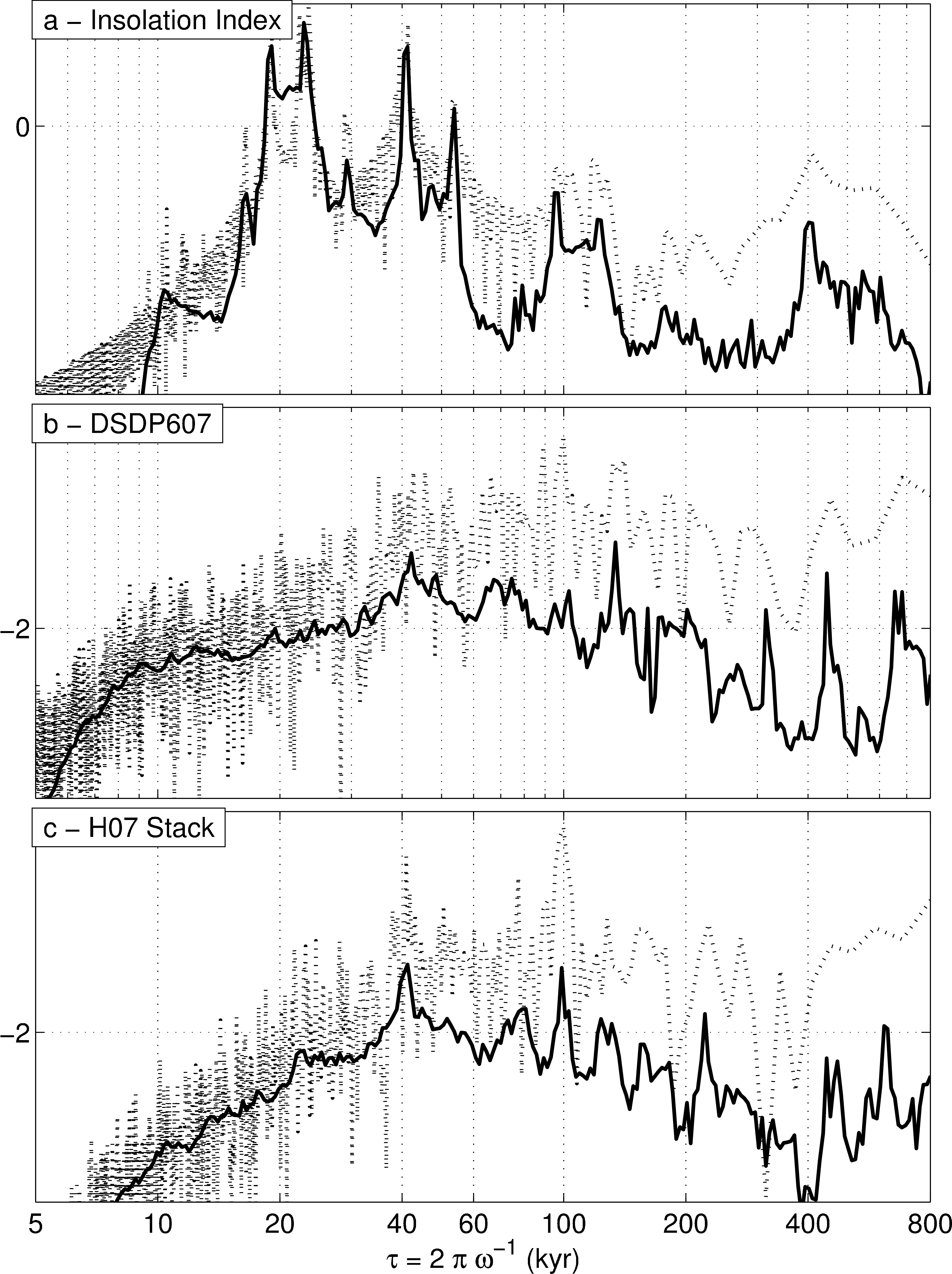
Figure 6.6: Comparison of Fourier magnitude (gray) and Synchrosqueezing magnitude averaged over the entire period (black) of (a) insolation index $f_{SF}$, and climate response in benthic ${\delta}^{18}O$ of (b) DSDP607 core, $f_{CR1}$, and (c) H07 stack, $f_{CR2}$. Synchrosqueezing averages are normalized by $1/R_{\psi}$ to correspond to the true signal magnitudes.

Synchrosqueezing analysis of the solar insolation index and benthic $\delta^{18}O$ makes a significant contribution in three important ways. First, it produces spectrally sharp traces of complex system evolution through the high-dimensional climate state space (compare with, e.g., [22, Fig. 2]). Second, it delineates the effects of noise on specific frequency ranges when comparing a single core to the stack. Low frequency components are mostly robust to noise induced by both local climate variability and the measurement process. Third, thanks to its precision, Synchrosqueezing allows the filtered reconstruction of signal components within frequency bands.

Questions about the key physical processes governing large scale climate variability over the last 2.5 Myr can be answered with sufficient accuracy only by precise data analysis and the development of a hierarchy of models at various levels of complexity that reproduce the key aspects of Pleistocene history. The resulting dynamic stochastic understanding of past climates may benefit our ability to predict future climates.

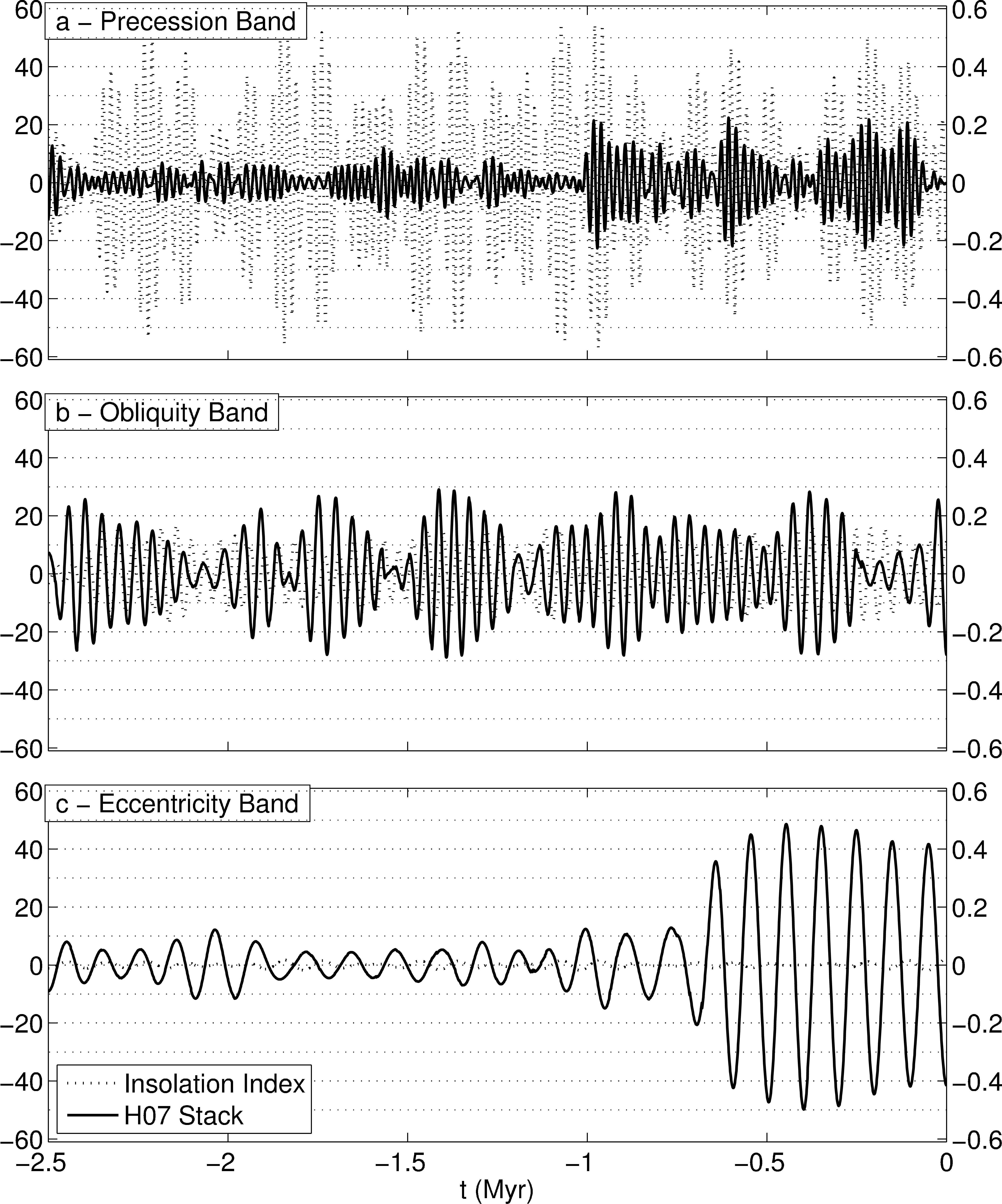
Figure 6.7: Milanković orbital components extracted by the inverse Synchrosqueezing transforms of insolation index $f_{SF}$ (gray curve with vertical scale on the left) and climate response in benthic ${\delta}^{18}O$ stack $f_{CR2}$ (black curve with vertical scale on the right) over (a) precession band (integrated from 17 kyr to 25 kyr), (b) obliquity band (40 kyr - 55 kyr), and (c) eccentricity band (90 kyr - 130 kyr).

Chapter 7 Multiscale Dictionaries of Slepian Functions on the Sphere

7.1 Introduction

The estimation and reconstruction of signals from their samples on a (possibly irregular) grid is an old and important problem in engineering and the natural sciences. Over the last several centuries, both approximation and sampling techniques have been developed to address this problem. Approximation theorems provide (possibly probabilistic) guarantees that a function can be approximated to a specified precision with a bounded number of coefficients in an alternate basis or frame. In general, such guarantees put constraints on the function (e.g., differentiability) and the domain (e.g., smoothness and compactness). Sampling theorems guarantee that a function can be reconstructed to a given precision from either point samples or some other form of sampling technique (e.g., linear combinations of point observations, as in the case of compressive sensing). Again, sampling theorems place requirements on both the sampling (e.g., grid uniformity or a minimum sampling rate), on the original function (e.g., a bandlimit), and/or on the domain (e.g., smoothness, compactness).

Approximation and sampling techniques are closely linked due to their similar goals. For example, a signal can be estimated via its representation in an alternate basis (e.g., via Riemannian sums that numerically calculate projections of point samples onto the basis functions). The estimate then follows by expanding the function in the given basis. Regularization (the approximation) of the estimate can be performed by excluding the basis elements assumed to be zero.

Figure 7.1: EMAG2: Earth Magnetic Anomaly Grid (nT), for the region covering Australia and New Zealand; reprinted from Fig. 6 of [69]. Note the higher frequency, locally directionally consistent components in the ocean basins, and the lower frequency components on the continents.

In this chapter, we focus on the approximation and sampling problem for subsets of the sphere ${\mathcal{R}}\subset S^{2}$. First, we are interested in the representation of signals that are bandlimited but whose contribution of higher frequencies arises from within a certain region of interest (ROI), denoted ${\mathcal{R}}$ (see, e.g., Fig. 7.1). Second, we are interested in reconstructing such functions from point samples within the ROI. To this end, we construct multiscale dictionaries of functions that are bandlimited on the sphere $S^{2}$ and space-concentrated in contiguous regions ${\mathcal{R}}$.

Our constructions are purely numerical, and are motivated by subdivision schemes for wavelet constructions on the interval. By construction, the functions have low coherency (their pairwise inner products are bounded in absolute value). As a result, thanks to new methods in sparse approximation (see, e.g., [15, 44]), they are good candidates for the approximation and reconstruction of signals that are locally bandlimited.

7.2 Notation and Prior Work

We will focus on the important prior work in signal representation, working our way up to Slepian functions on the sphere — the functions upon which our construction is based.

Before proceeding, we first introduce some notation. For two sequences (vectors) $\widehat{f},\widehat{g}\in\ell^{2}$ and a subset of the natural numbers $\Omega$, we refer to the product ${\left\langle{\widehat{f}},{\widehat{g}}\right\rangle_{\Omega}=\sum_{i\in\Omega}\widehat{f}_{i}\overline{\widehat{g}_{i}}}$. When $\Omega$ is omitted, we assume the sum is over all indices. The norm of $\widehat{f}$ is denoted ${{\left\lVert\widehat{f}\right\rVert_{\Omega}^{2}=\left\langle{\widehat{f}},{\widehat{f}}\right\rangle}_{\Omega}}$. For square-integrable functions $f$ and $h$ on a Riemannian manifold $({\mathcal{M}},g)$ (that is, $f,h\in L^{2}({\mathcal{M}})$), and ${\mathcal{R}}$ some subset of ${\mathcal{M}}$, we denote the inner product ${\left\langle{f},{h}\right\rangle_{\mathcal{R}}=\int_{\mathcal{R}}f(x)\overline{h(x)}d\mu(x)}$, where $d\mu(x)$ is the volume element associated with the metric $g$ (see Apps. A–B). The norm is again defined as ${\left\lVert f\right\rVert_{\mathcal{R}}=\sqrt{\left\langle{f},{f}\right\rangle}_{\mathcal{R}}}$. The type of inner product, manifold, and metric will be clear from the context. Notation referring specifically to functions on the sphere $S^{2}$ and the spherical harmonics may be found in §B.2.2.

The prior literature in this area pertains to sampling, interpolation, and basis functions on the real line, and we focus on these next.

7.2.1 Reconstruction of Bandlimited, Regularly Sampled Signals on ${\mathbb{R}}$

A signal $f(t)$ on the real line is defined as bandlimited when it has no frequencies higher than some bandlimit $W$. That is, $\widehat{f}(\omega)=0$ for $\left\lvert\omega\right\rvert>W$. The simplest version of the sampling theorem, as given by Shannon [89, §II], states that if $f$ is sampled at regular intervals of with a frequency at or above the sampling limit $t_{s}=1/2W$, it can be exactly reconstructed via convolution with the sinc low-pass filter:

$$f(t)=\sum_{n=-\infty}^{\infty}x_{n}\text{sinc}(2Wt-n),$$ (7.1)

where $x_{n}=f(t_{s}n)$ are the samples and $\text{sinc}(z)=\sin(\pi z)/(\pi z)$.

Shannon also heuristically describes [89, §III] that if a bandlimited function $f$, with bandlimit $W$, is also timelimited to an interval $[-T,T]$ (that is, all of its samples, taken at rate $k_{s}$, are exactly 0 outside of this interval), then it requires $N=\left\lfloor 2TW\right\rfloor$ samples on this interval to reconstruct. Thus a function that is both time- and bandlimited as described above can be described using only $N$ numbers—and the dimension of such functions is $N$, which is called the Shannon number.

Shannon’s heuristic definition was based on the (at that time) well-known fact that a bandlimited, substantially spacelimited function can be represented well with $N$ numbers. In fact, it is impossible to construct exactly space- and frequency- limited functions on the line; see, e.g., the Paley-Wiener theorem [86, Thm. 7.22]. Thus a different technique is needed for the estimation of bandlimited functions on an interval, from samples only within that interval. As we will describe next the optimal representation for this $N$-dimensional space is given by the ordered basis of Slepian functions. We will now focus on the construction of Slepian functions, and will provide a more rigorous definition of the Shannon number for the space of bandlimited, space-concentrated functions.

7.2.2 An Optimal Basis for Bandlimited Functions on the Interval

The estimation of bandlimited signals on an interval requires the construction of an optimal basis to represent such functions. The Prolate Spheroidal Wave Functions (PSWF) [61, 62, 99], also known as Slepian functions, are one such basis. The criterion of optimal concentration is with respect to the ratio of $L^{2}$ norms. Let ${\mathcal{R}}=[-T,T]$ be the interval on the line, and $\Omega=[-W,W]$ be the bandlimit in frequency. The PSWF are the orthogonal set of solutions to the variational problem

$$\operatorname*{maximize}_{g\in L^{2}({\mathbb{R}})}\quad \lambda=\frac{\int_{\mathcal{R}}g^{2}(t)dt}{\int_{\mathbb{R}}g^{2}(t)dt},$$ (7.2)

subject to $$\hat{g}(\omega)=0,\quad\omega\not\in\Omega,$$

where for $\alpha=1,2,\ldots$, the value $\lambda_{\alpha}$ is achieved by $g_{\alpha}$, and we impose the orthonormality constraint $\left\langle{g_{\alpha}},{g_{\alpha^{\prime}}}\right\rangle=\delta_{\alpha\alpha^{\prime}}$. Here $\lambda_{\alpha}$ is the measure of concentration of $g_{\alpha}$ on ${\mathcal{R}}$; these eigenvalues are bounded: $0<\lambda_{\alpha}<1$. We use the standard ordering of the Slepian functions, wherein ${\lambda_{1}>\lambda_{2}>\cdots}$ (the first Slepian function is the most concentrated within ${\mathcal{R}}$, the second is the second most concentrated, and so on).

The orthonormal solutions to (7.2) satisfy the integral eigenvalue problem [99, 93]:

$$\int_{\Omega} K_{F}(\omega,\omega^{\prime})\widehat{g}_{\alpha}(\omega^{\prime})d\omega^{\prime}=\lambda_{\alpha}\widehat{g}_{\alpha}(\omega),\ \omega\in\Omega,\quad\text{where}$$ (7.3)

$$K_{F}(\omega,\omega^{\prime})=\frac{\sin T(\omega-\omega)}{\pi(\omega-\omega^{\prime})}.$$

Note that $K_{F}$ is a smooth, symmetric, positive-definite kernel with eigenfunctions $\left\{\widehat{g}_{\alpha}\right\}_{\alpha}$ (and associated eigenvalues $\left\{\lambda_{\alpha}\right\}_{\alpha}$). Mercer’s theorem therefore applies [82, §97,98], and we can write

$$K_{F}(\omega,\omega^{\prime})=\sum_{a\geq 1}\lambda_{\alpha}\widehat{g}_{\alpha}(\omega)\overline{\widehat{g}_{\alpha}(\omega^{\prime})}\qquad\text{and}\qquad K_{F}(\omega,\omega)=\sum_{a\geq 1}\lambda_{\alpha}\left\lvert\widehat{g}_{\alpha}(\omega)\right\rvert^{2}.$$ (7.4)

In practice, (7.3) can be solved exactly and efficiently using a special “trick”: this integral equation commutes with a special second-order differential operator and thus its solution can be found via the solution of a PDE of Sturm-Liouville type. The values of the $g_{\alpha}$’s, or of the $\widehat{g}_{\alpha}$’s, can be evaluated exactly at any set of points on their domains, via the factorization of a special tridiagonal matrix [90, 98]. This construction is beyond the scope of this chapter.

It has been shown that the Slepian functions are all either very well concentrated within the interval, or very well concentrated outside of it. That is, the eigenvalues of the Slepian functions are all either nearly $1$ or nearly $0$ [99, Table 1]. Furthermore the values of any bandlimited signal with concentration $1-\epsilon$ on the interval, can be estimated to within a squared error (in $L^{2}$) bounded by $\epsilon$, for any arbitrarily $\epsilon>0$, by approximating this signal using a linear combination of all the Slepian functions whose eigenvalues are near unity [62, Thm. 3], and no fewer [62, Thm. 5].

The number of Slepian functions required to approximate a bandlimited, space-concentrated function can be therefore be calculated by summing their energies:

$$N_{T,W}=\sum_{\alpha\geq 1}\lambda_{\alpha}=\sum_{\alpha\geq 1}\lambda_{\alpha}\int_{\Omega}\left\lvert\widehat{g}_{\alpha}(\omega)\right\rvert^{2}d\omega=\int_{\Omega}K_{F}(\omega,\omega)d\omega=\frac{2TW}{\pi},$$ (7.5)

where we used (7.4) after swapping the sum and integral.

The difference between this value of $N$ and Shannon’s version is due to changes in normalization of Fourier transforms and the constant $\pi$ inside the $\sin$ in (7.1).

7.2.3 An Optimal Basis for Bandlimited Functions on subregions of the Sphere $S^{2}$

The construction of Slepian functions on the sphere proceeds similarly to the interval case, with differences due to the compactness of $S^{2}$. Let ${\mathcal{R}}$ be a closed and connected subset of $S^{2}$ and let the frequency bandlimit be ${\Omega=\left\{(l,m):0\leq l\leq L,-l\leq m\leq l\right\}}$. The set of square-integrable functions on $S^{2}$ with bandlimit $\Omega$, which we will call $L^{2}_{\Omega}(S^{2})$, is an $(L+1)^{2}$ dimensional space. This follows because any $f\in L^{2}_{\Omega}(S^{2})$ can be written as

$$f(\theta,\phi)=\sum_{l=0}^{L}\sum_{m=-l}^{l}\widehat{f}_{lm}Y_{lm}(\theta,\phi),$$ (7.6)

and therefore

$$\dim L^{2}_{\Omega}(S^{2})=\sum_{l=0}^{L}(2l+1)=(L+1)^{2}.$$

For the rest of the chapter, we will refer to the bandlimits “$\Omega$” and “$L$” interchangeably.

We now proceed as in [93]. Slepian functions concentrated on ${\mathcal{R}}$ with bandlimit $L$ are the orthogonal set of solutions to the variational problem

$$\operatorname*{maximize}_{g\in L^{2}(S^{2})}\quad \lambda=\frac{\int_{\mathcal{R}}g^{2}(x)d\mu(x)}{\int_{S^{2}}g^{2}(x)d\mu(x)},$$ (7.7)

subject to $$\hat{g}_{lm}=0,\quad(l,m)\not\in\Omega,$$

where the value $\lambda_{\alpha}$ is achieved by $g_{\alpha}$, $\alpha=1,2,\ldots$, and we impose the orthonormality constraint

$$\int_{S^{2}}g_{\alpha}(x)g_{\alpha^{\prime}}(x)d\mu(x)=\delta_{\alpha\alpha^{\prime}}.$$ (7.8)

Finally, as before, we use the standard order for the Slepian functions: ${\lambda_{1}\geq\lambda_{2}\geq\cdots}$ (i.e., in decreasing concentration). Note that in contrast to the 1D case, the concentration inequalities are not strict due to possible geometric degeneracy. Due to orthonormality, the Slepian functions also fulfill the orthogonality constraint

$$\int_{{\mathcal{R}}}g_{\alpha}(x)g_{\alpha^{\prime}}(x)d\mu(x)=\lambda_{\alpha}\delta_{\alpha\alpha^{\prime}}.$$ (7.9)

The problem (7.7) admits an integral formulation equivalent to (7.3). In addition, as the Fourier basis on $S^{2}$ is countable, the construction can be reduced to a matrix eigenvalue problem.

Writing $g$ in (7.7) via its Fourier series, as in (7.6), reduces the problem to [90, Eq. 33]

$$\sum_{(l^{\prime},m^{\prime})\in\Omega} K_{lm,l^{\prime}m^{\prime}}\widehat{g}_{l^{\prime}m^{\prime}}=\lambda\widehat{g}_{lm},\quad(l,m)\in\Omega,$$ (7.10)

where $$K_{l^{\prime}m^{\prime},lm}=\left\langle{Y_{lm}},{Y_{l^{\prime}m^{\prime}}}\right\rangle_{\mathcal{R}}.$$

From now on, we will denote by $K$ the $(L+1)^{2}{\times}(L+1)^{2}$ matrix with coefficients $K_{l^{\prime}m^{\prime},lm}$. The vector $K\widehat{g}$ is thus an $(L+1)^{2}$-element vector, indexed by coefficients $(l,m)$, with $(K\widehat{g})_{lm}=\sum_{(l^{\prime},m^{\prime})\in\Omega}K_{lm,l^{\prime}m^{\prime}}\widehat{g}_{l^{\prime}m^{\prime}}$ for any $(l,m)\in\Omega$. The matrix $K$ is called the spectral localization kernel; it is real, symmetric and positive-definite. We can now rewrite (7.7) as a proper eigenvalue problem: we solve

$$K\widehat{G}=\widehat{G}\Lambda$$ (7.11)

where $\widehat{G}=\left(\widehat{g}_{1}~{}\cdots~{}\widehat{g}_{(L+1)^{2}}\right)$ is the orthonormal matrix of eigenvectors and the diagonal matrix $\Lambda$ is composed of eigenvalues in decreasing order: ${\Lambda=\text{diag}\left(\lambda_{1}~{}\lambda_{2}~{}\cdots~{}\lambda_{(L+1)^{2}}\right)}$. As $K$ is positive-definite and symmetric, its eigenvectors, ${\widehat{g}_{\alpha},~{}\alpha=1,2,\cdots,(L+1)^{2}}$, form an orthogonal set that spans the space $L^{2}_{\Omega}(S^{2})$. The spatial functions can be easily calculated via (7.6) and efficient recursion formulas for the spherical harmonics.

The Shannon number, $N_{\left\lvert{\mathcal{R}}^{\prime}\right\rvert,L}$ is again defined as the sum of the eigenvalues,

$$N_{\left\lvert{\mathcal{R}}^{\prime}\right\rvert,L}=\sum_{\alpha=1}^{(L+1)^{2}}\lambda_{\alpha}=\text{Tr}(\Lambda)=\text{Tr}(\widehat{G}).$$ (7.12)

It can also be shown (see, e.g., [93, §4.3]) that the Shannon number is given by a formula similar to (7.5):

$$N_{\left\lvert{\mathcal{R}}^{\prime}\right\rvert,L}=\frac{\left\lvert{\mathcal{R}}^{\prime}\right\rvert}{4\pi}(L+1)^{2},$$ (7.13)

where $\left\lvert{\mathcal{R}}^{\prime}\right\rvert=\int_{x\in{\mathcal{R}}^{\prime}}d\mu(x)$ is the area of ${\mathcal{R}}^{\prime}$.

7.2.4 Calculation of the Spectral Localization Kernel $K$

In contrast to the 1D construction of §7.2.2, and with the exception of the cases when the domain ${\mathcal{R}}$ has azimuthal and/or equatorial symmetry (see, e.g., [93]), there is no known differential operator that commutes with the spatial integral version of (7.10). Nevertheless, thanks to the discrete nature of the problem, we can find tractable solutions using simple numerical analysis.

We now briefly discuss the calculation of the symmetric positive-definite matrix $K$ of (7.10); basing the discussion on the work in [92, §4.2]. As the calculation of the largest eigenvalues and associated eigenvectors of $K$ can be performed using standard efficient iterative solvers, the main computational complexity lies in constructing the matrix itself.

The problem of calculating $K$ reduces to numerically estimating the constrained spatial inner product between spherical harmonics,

$$K_{lm,l^{\prime}m^{\prime}}=\int_{\mathcal{R}}Y_{lm}(x)Y_{l^{\prime}m^{\prime}}(x)d\mu(x),$$ (7.14)

when we are given the (splined) boundary $\partial{\mathcal{R}}$ (a closed simple curve in $S^{2}$). This is performed via a semi-analytic integration over a grid. We first find the northernmost and southernmost colatitudes, $\theta_{n}$ and $\theta_{s}$, of $\partial{\mathcal{R}}$. For a given colatitude $\theta$, we can find the westernmost and easternmost points, $\phi_{e}(\theta)$ and $\phi_{w}(\theta)$ of $\partial{\mathcal{R}}$. If ${\mathcal{R}}$ is nonconvex, there will be some $I(\theta)$ number of such points, which we denote $\phi_{e,i}(\theta)$ and ${\phi_{w,i}(\theta),i=1,\ldots,I(\theta)}$. The integral (7.14) thus becomes

$$K_{lm,l^{\prime}m^{\prime}} =\int_{\theta_{s}}^{\theta_{n}}X_{lm}(\theta)X_{l^{\prime}m^{\prime}}(\theta)\Phi_{mm^{\prime}}(\theta)\sin\theta d\theta,$$ (7.15)

$$\text{where}\quad\Phi_{mm^{\prime}}(\theta) =\sum_{i=1}^{I(\theta)}\int_{\phi_{e,i}(\theta)}^{\phi_{w,i}(\theta)}{\mathsf{N}}_{m}{\mathsf{N}}_{m^{\prime}}{\mathsf{S}}_{m}(\phi){\mathsf{S}}_{m^{\prime}}(\phi)d\phi,$$ (7.16)

$${\mathsf{N}}_{m} =\sqrt{2-\delta_{0m}},$$

$$\text{and}\quad{\mathsf{S}}_{m}(\phi) =\begin{cases}\cos m\phi&\text{if }m\leq 0,\\ \sin m\phi&\text{if }m>0.\end{cases}$$

Above, $X_{lm}$ is the colatitudinal portion of $Y_{lm}$; for more details, see App. B.

Equation (7.15) is calculated via Gauss-Legendre integration using the Nyström method, first by discretizing the colatitudinal integral into $J$ points $\left\{\theta_{j}\right\}_{j=1}^{J}$, and then evaluating the integral (7.16) analytically at each point $\theta_{j}$. The discretization number $J$ for the numerical integration is chosen large enough that the spatial-domain eigenfunctions, as calculated via the diagonalization of $K$ and application of (7.6), satisfy the Slepian orthogonality relations (7.8) and (7.9) to within machine precision.

A second way involves the expansion of $\left\langle{Y_{lm}},{Y_{l^{\prime}m^{\prime}}}\right\rangle$ into spherical harmonics — the expansion coefficients are the quantum-mechanical Wigner $3j$ functions, which can be calculated recursively. The remaining integral over a single spherical harmonic can be performed recursively in the manner of [78], which is exact. See also [37].

7.3 Multiscale Trees of Slepian Functions

We now turn our focus to numerically constructing a dictionary ${\mathcal{D}}$ of functions that can be used to approximate mostly low bandwidth signals on the sphere. As we will see in the next section, this dictionary allows for the reconstruction of a variety of signals from their point samples.

To construct ${\mathcal{D}}$, we first need some definitions. Let ${\mathcal{R}}\subset S^{2}$ be a simply connected subset of the sphere. Let $L$ be the bandwidth: the dictionary ${\mathcal{D}}$ will be composed of functions bandlimited to harmonic degrees $0\leq l\leq L$. The construction is based on a binary tree. Choose a positive integer (the node capacity) $n_{b}$; each node of the tree corresponds to the first $n_{b}$ Slepian functions with bandlimit $L$ and concentrated on a subset ${\mathcal{R}}^{\prime}\subset{\mathcal{R}}$. The top node of the tree corresponds to the entire region ${\mathcal{R}}$, and each node’s children correspond to a division of ${\mathcal{R}}^{\prime}$ into two roughly equally sized subregions (the subdivision scheme will be described soon). As the child nodes will be concentrated in disjoint subsets of ${\mathcal{R}}^{\prime}$, all of their corresponding functions and children are effectively incoherent.

Figure 7.2: The binary tree subdivision scheme and associated dictionary ${\mathcal{D}}_{{\mathcal{R}},L}$. We define the top-level region ${\mathcal{R}}$ as ${\mathcal{R}}^{(1)}$ and the generic subsets ${\mathcal{R}}^{\prime}$ as $R^{(j)}$.

We now fix a height $H$ of the tree: the number of times to subdivide ${\mathcal{R}}$. The height is determined as the maximum number of binary subdivisions of ${\mathcal{R}}$ that can have $n_{b}$ well concentrated functions. That is, we find the minimum integer $H$ such that

$$n_{b}\geq N_{2^{-H}\left\lvert{\mathcal{R}}\right\rvert,L}$$

with the solution

$$H=\left\lceil\log_{2}\left(\frac{\left\lvert{\mathcal{R}}\right\rvert}{4\pi}\frac{(L+1)^{2}}{n_{b}}\right)\right\rceil.$$

A complete binary tree with height $H$ has $2^{H+1}-1$ nodes, so from now on we will denote the dictionary

$${\mathcal{D}}_{{\mathcal{R}},L,n_{b}}=\left\{d^{(1,1)},d^{(1,2)},\cdots,d^{(1,n_{b})},\cdots,d^{\left(2^{H+1}-1,1\right)},\cdots,d^{\left(2^{H+1}-1,n_{b}\right)}\right\}$$

as the set of $\left\lvert{\mathcal{D}}_{{\mathcal{R}},L,n_{b}}\right\rvert=n_{b}\,(2^{H+1}-1)$ functions thus constructed on region ${\mathcal{R}}$ with bandlimit $L$ and node capacity $n_{b}$. Fig. 7.2 shows the tree diagram of the subdivision scheme. We use the standard enumeration of nodes wherein node $(j,\cdot)$ is subdivided into child nodes $(2j,\cdot)$ and $(2j+1,\cdot)$, and at a level $0\leq h\leq H$, the nodes are indexed from $2^{h}\leq j\leq 2^{h+1}-1$. More specifically, for ${j=1,2,\ldots}$, we have ${{\mathcal{R}}^{(j)}={\mathcal{R}}^{(2j)}\cup{\mathcal{R}}^{(2j+1)}}$. Furthermore, letting $g^{{\mathcal{R}}^{\prime}}_{\alpha}$ be the $\alpha$’th Slepian function on ${\mathcal{R}}^{\prime}$ (the solution to (7.7) with concentration region ${\mathcal{R}}^{\prime}$), we have that

$$d^{(j,\alpha)}=g^{{\mathcal{R}}^{(j)}}_{\alpha}.$$

Fig. 7.3 shows an example of the construction when ${\mathcal{R}}$ is the African continent. Note how, for example, $d^{(4,1)}$ and $d^{(5,1)}$ are the first Slepian functions associated with the subdivided domains of ${\mathcal{R}}^{(2)}$.

(a) $d^{(1,1)}$

(b) $d^{(2,1)}$

(c) $d^{(3,1)}$

(d) $d^{(4,1)}$

(e) $d^{(5,1)}$

(f) $d^{(6,1)}$

(g) $d^{(250,1)}$

(h) $d^{(251,1)}$

(i) $d^{(252,1)}$

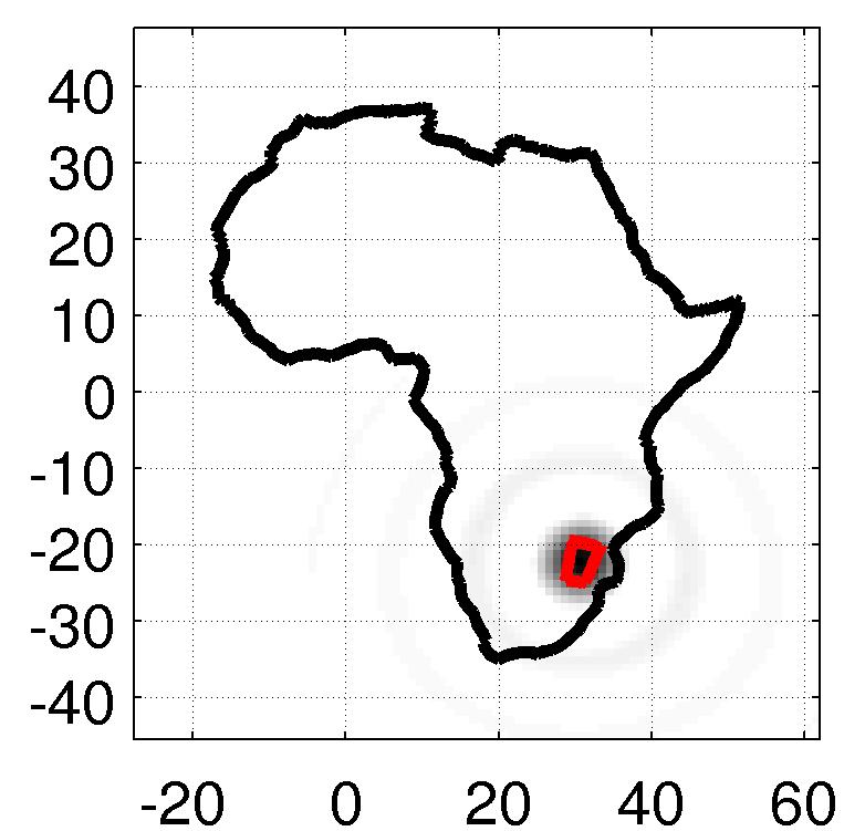
(j) $d^{(253,1)}$

(k) $d^{(254,1)}$

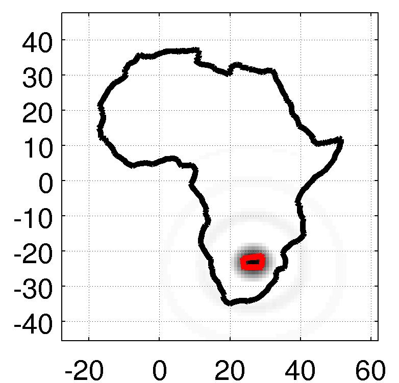
(l) $d^{(255,1)}$

Figure 7.3: Slepian Tree Dictionary ${\mathcal{D}}_{\text{Africa},36,1}$ (having size $\left\lvert{\mathcal{D}}\right\rvert=255$); functions $d^{(1,1)}$ through $d^{(6,1)}$ and $d^{(250,1)}$ through $d^{(255,1)}$. The x-axis is longitude, the y-axis is colatitude. Regions of concentration $\left\{{\mathcal{R}}^{(i)}\right\}$ are outlined.

To complete the top-down construction, it remains to decide how to subdivide a region ${\mathcal{R}}^{\prime}$ into equally sized subregions. For roughly circular connected domains, the first Slepian function has no sign changes, and the second Slepian function has a single zero-level curve that subdivides the region into approximately equal areas; when ${\mathcal{R}}^{\prime}$ is a spherical cap, the subdivision is exact [93]. We thus subdivide a region ${\mathcal{R}}^{\prime}$ into the two nodal domains associated with the second Slepian function on that domain; see Fig. 7.4 for a visualization of the subdivision scheme as applied to the African continent.

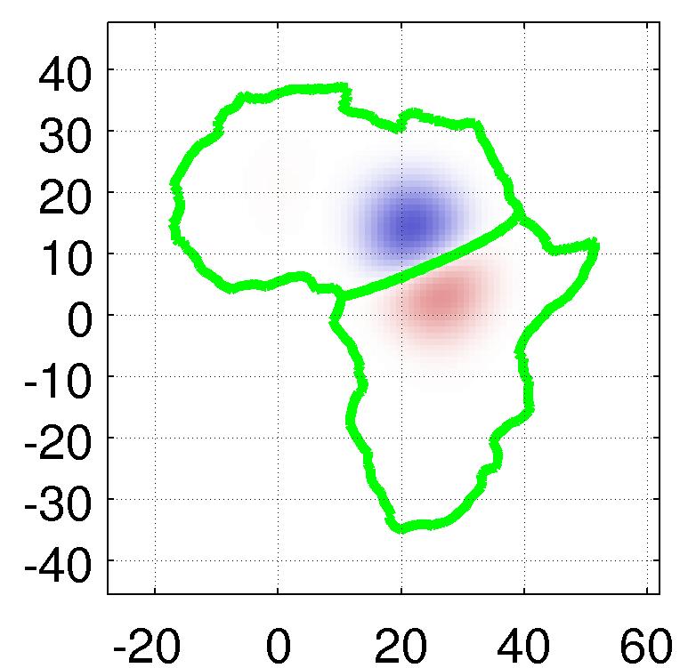
(a) $d^{(1,2)}$

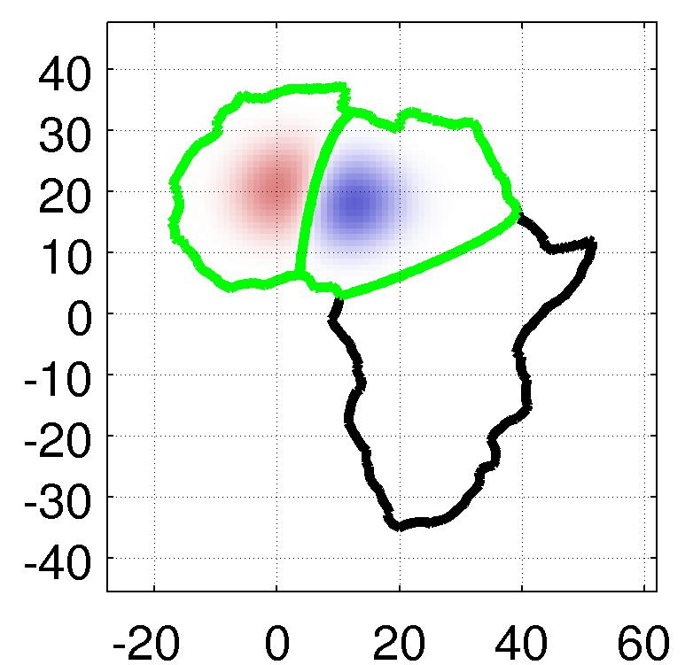
(b) $d^{(2,2)}$

(c) $d^{(3,2)}$

(d) $d^{(4,2)}$

(e) $d^{(5,2)}$

(f) $d^{(6,2)}$

Figure 7.4: Second Slepian functions associated with the regions in Figs. 7.3(a-f). The x-axis is longitude, the y-axis is colatitude. Regions of concentration, and the central dividing contour (the zero-level set), are drawn in green. Blue and red represent the sign of the Slepian function values.

7.4 Concentration, Range, and Incoherence

The utility of the Tree construction presented above depends on its ability to represent bandlimited functions in a region ${\mathcal{R}}$, and its efficacy at reconstructing functions from point samples in ${\mathcal{R}}$. These properties, in turn, reduce to questions of concentration, range, and incoherence:

• Dictionary ${\mathcal{D}}$ is concentrated in ${\mathcal{R}}$ if its functions are concentrated in ${\mathcal{R}}$.

• The range of dictionary ${\mathcal{D}}$ is the subspace spanned by its elements. Ideally, the basis formed by the first $N$ Slepian functions on ${\mathcal{R}}$ is a subspace of the range of ${\mathcal{D}}$.

• When ${\mathcal{D}}$ is incoherent, pairwise inner products of its elements have low amplitude: pairs of functions are approximately orthogonal. This, in turn, is a useful property when using ${\mathcal{D}}$ to estimate signals from point samples, as we will see in the next section.

In this section, we provide several techniques for analyzing these properties for a given dictionary ${\mathcal{D}}$, providing numerical examples as we go along.

Unlike the eigenvalues of the Slepian functions on ${\mathcal{R}}$, not all of the eigenvalues of the elements of ${\mathcal{D}}_{{\mathcal{R}}}$ reflect their concentration within this top-level (parent) region. We thus define the modified concentration value

$$\nu^{(j,\alpha)}=\int_{{\mathcal{R}}}\left[d^{(j,\alpha)}(x)\right]^{2}d\mu(x).$$ (7.17)

Recalling that $\left\lVert d^{(j,\alpha)}\right\rVert_{2}=1$, the value $\nu$ is simply the percentage of energy of the $(j,\alpha)^{\text{th}}$ element that is concentrated in ${\mathcal{R}}$. This value is always larger than the element’s eigenvalue, which relates its fractional energy within the smaller subset ${\mathcal{R}}^{(j)}$. Figs. 7.5, 7.6, and 7.7 compare the eigenvalues of the Slepian functions on the African continent with those of the Tree construction, as well as with numerically calculated values of $\nu$.

Figure 7.5: Eigenvalues of the first $N_{\text{Africa},36}$ Slepian functions for the African continent, normalized and on a base-10 log scale. Blue lines correspond to integer multiples of the Shannon number ${N_{\text{Africa},36}\approx 79}$.

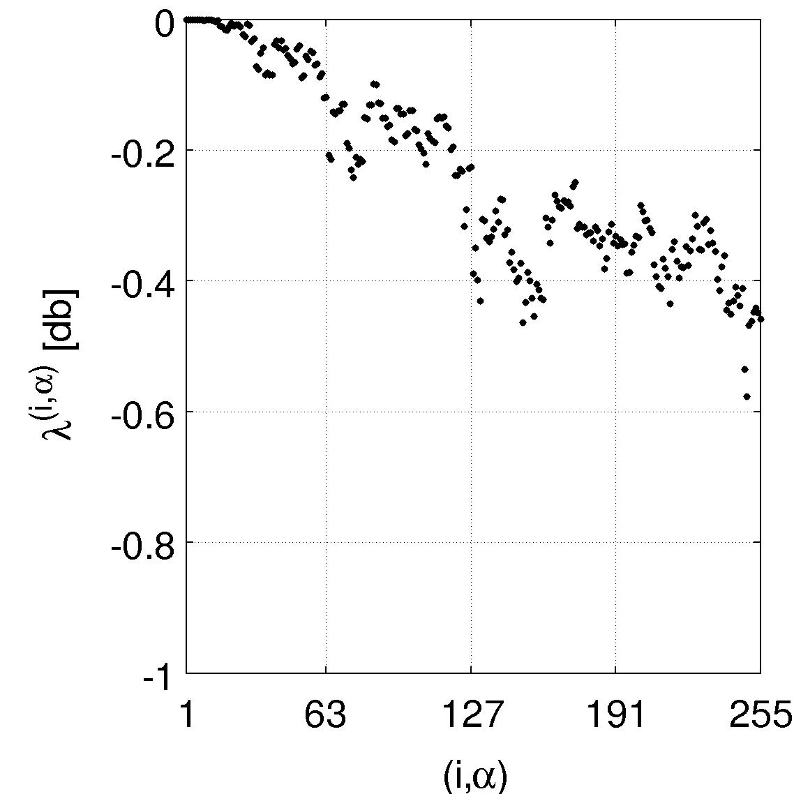
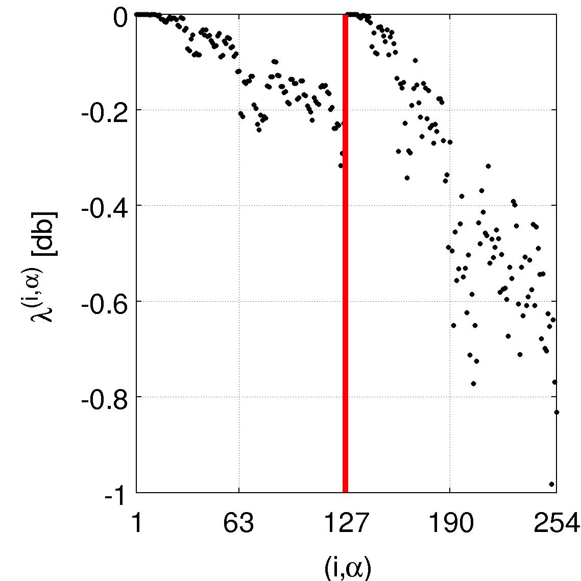
Figure 7.6: Eigenvalues of the dictionary elements of ${{\mathcal{D}}}_{\text{Africa},36,1}$ (left) and ${{\mathcal{D}}}_{\text{Africa},36,2}$ (right), normalized and on a base-10 log scale. On the right pane, the thick line separates the 127 elements with $\alpha=1$ (left) and $\alpha=2$ (right).

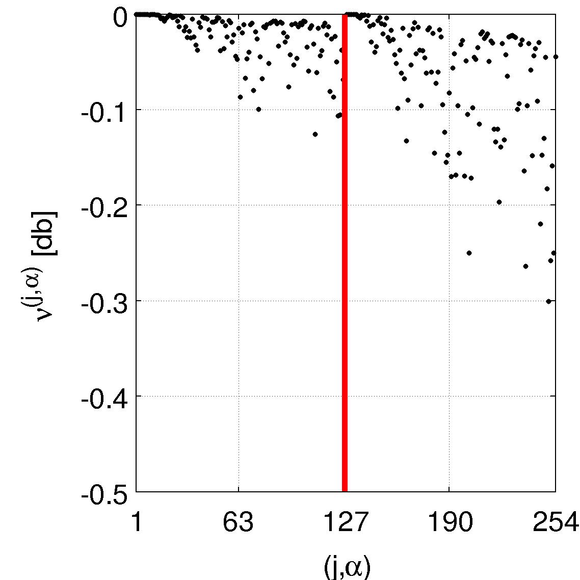
Figure 7.7: Concentrations $\nu$ of the dictionary elements of ${{\mathcal{D}}}_{\text{Africa},36,1}$ (left) and ${{\mathcal{D}}}_{\text{Africa},36,2}$ (right), normalized and on a base-10 log scale. On the right pane, the thick line separates the 127 elements with $\alpha=1$ (left) and $\alpha=2$ (right).

The size of dictionary ${\mathcal{D}}_{{\mathcal{R}},L,n_{b}}$ is generally larger than the Shannon number $N_{\left\lvert{\mathcal{R}}\right\rvert,L}$ for any node capacity $n_{b}$, and as a result it cannot form a proper basis (it has too many functions). Ideally, then, we require that elements of the range of the dictionary spans the space of the first $N_{\left\lvert{\mathcal{R}}\right\rvert,L}$ Slepian functions. We discuss two visual approaches for determining if this is the case.

Though the spatial nature of the construction makes it clear that dictionary elements tend to cover the entire domain ${\mathcal{R}}$, we also investigate the spectral energies of these elements; and compare them with the energies of the $N_{\left\lvert{\mathcal{R}}\right\rvert,L}$ Slepian functions on ${\mathcal{R}}$, which “essentially” form a basis for bandlimited functions in ${\mathcal{R}}$. The spectral energy density of a function $f$ is given for each degree ${l=0,\ldots,L}$ by [27, Eq. 38]:

$$S^{f}_{l}=\frac{1}{2l+1}\sum_{m=-l}^{l}\left\lvert\widehat{f}_{lm}\right\rvert^{2}.$$

Figs. 7.8 and 7.9 compare the power spectra of the Slepian functions on the African continent with the power spectra of two dictionaries given by the tree construction. While the Slepian functions are concentrated within specific ranges of the harmonics, the tree construction leads to spectra that depend on the degree. The dictionary elements with $\alpha=1$ tend to either contain mainly low-frequency harmonics or, for elements concentrated on smaller regions, have a more flat harmonic response within the bandlimit. Dictionary elements associated with higher order Slepian functions have a more pass-band response when concentrated on larger regions and a more flat response within the higher frequencies of the bandlimit when concentrated on smaller regions. So while it is clear that the Slepian functions span the bandlimited frequencies, the spectral amplitude plots do not relay this as clearly for the tree construction.

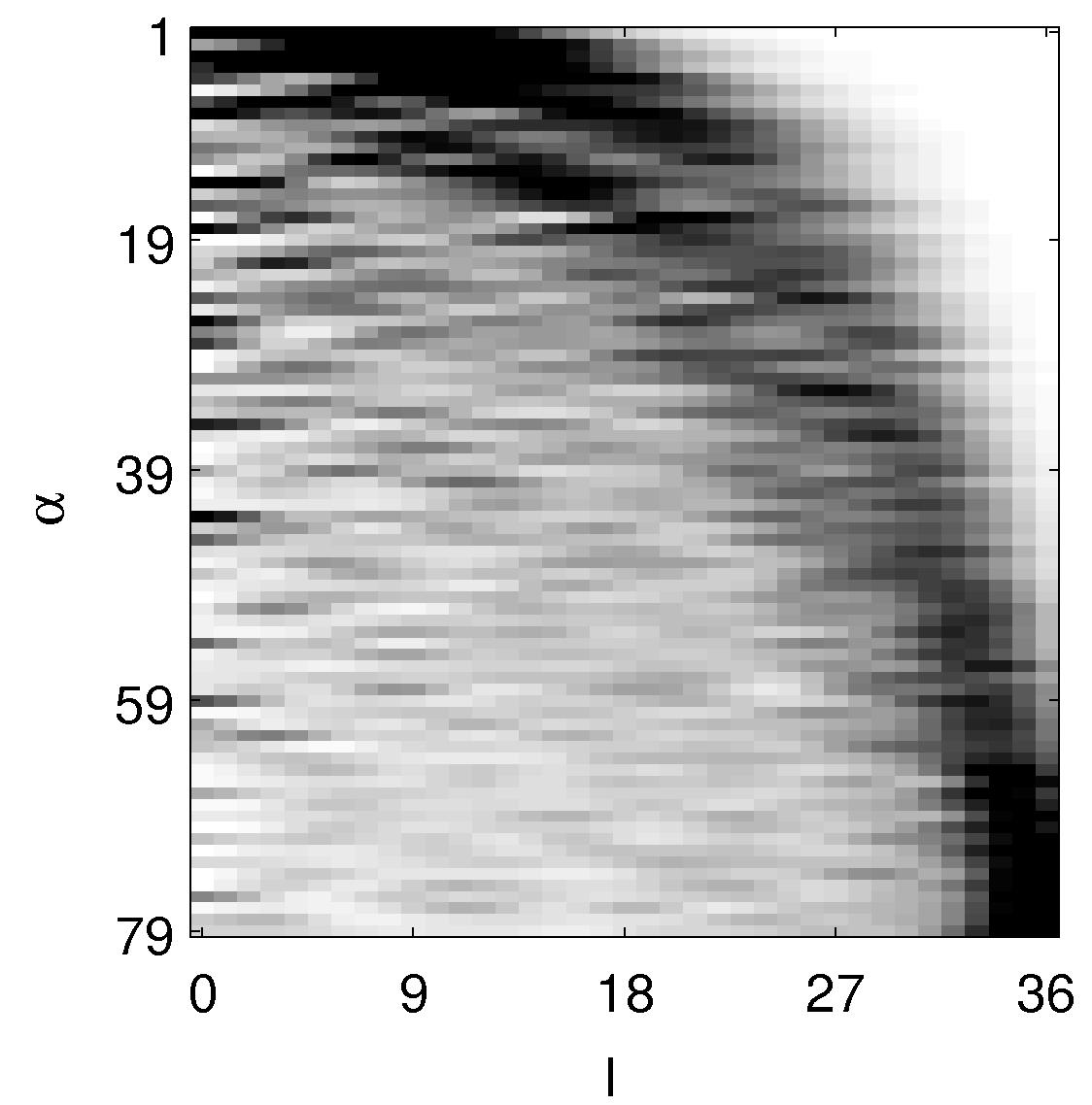
Figure 7.8: Power Spectrum $S_{l}$ of the first $N_{\text{Africa},36}$ Slepian functions for the African continent. The x-axis is degree $l$, the y-axis is Slepian function index $\alpha$. Values are between 0 (white) and 1 (black).

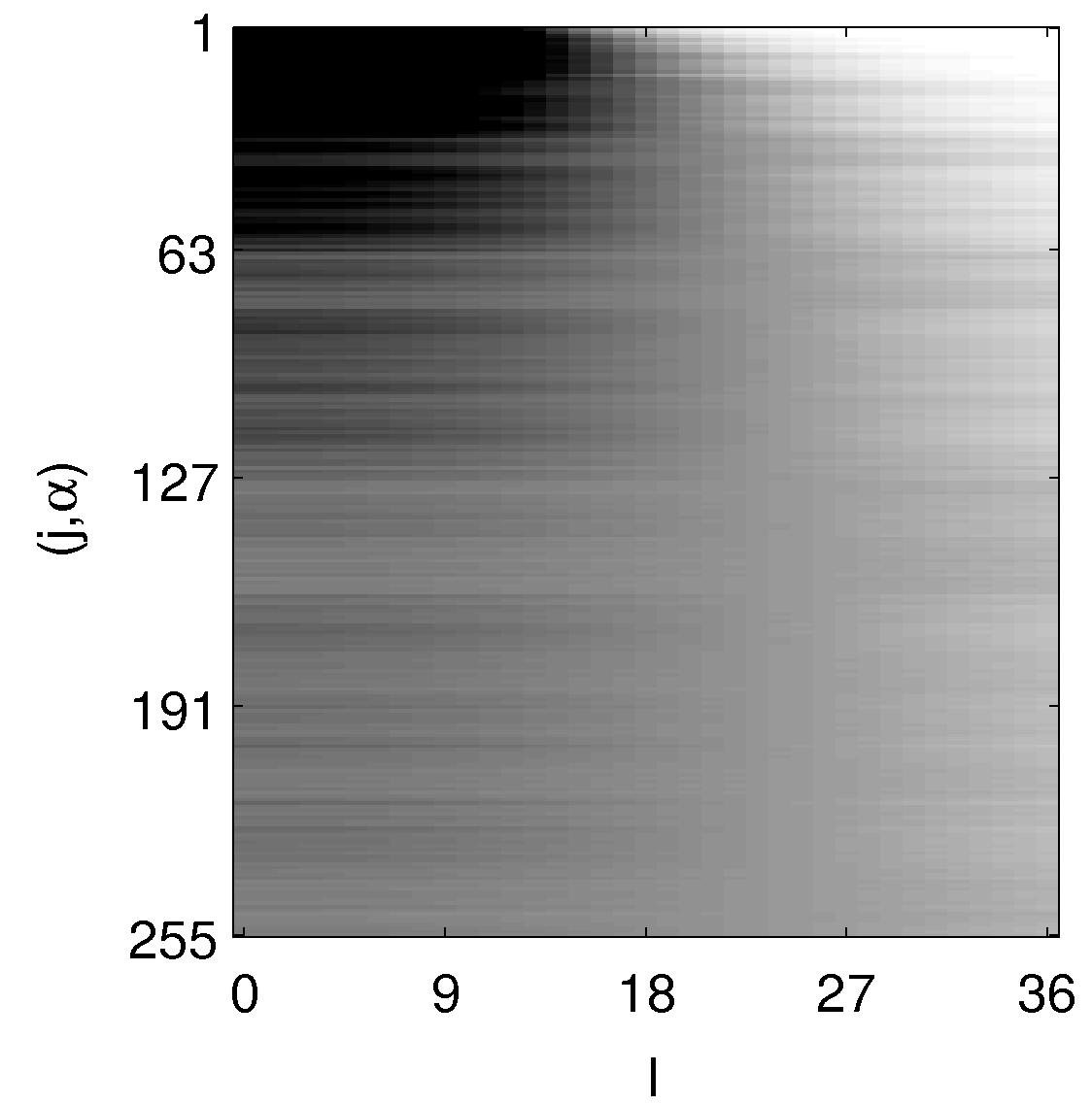
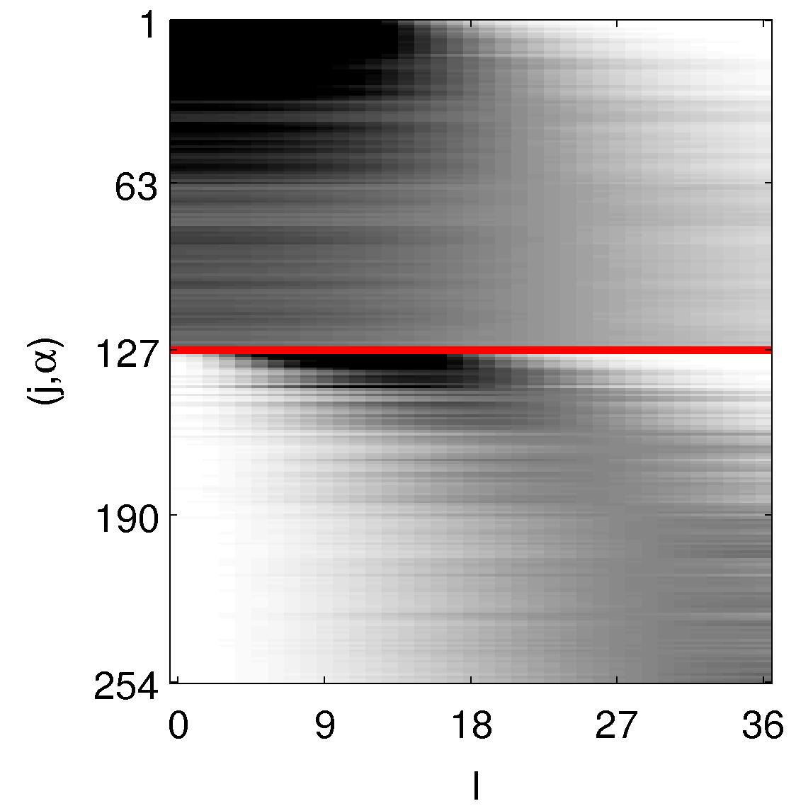
Figure 7.9: Power Spectra $S_{l}$ of the elements of the dictionaries ${{\mathcal{D}}}_{\text{Africa},36,1}$ (left) and ${{\mathcal{D}}}_{\text{Africa},36,1}$ (right). The x-axis is degree $l$, the y-axis is dictionary index $(j,\alpha)$. On the right pane, the red line separates the 127 elements with $\alpha=1$ (top) and $\alpha=2$ (bottom). Values are between 0 (white) and 1 (black).

A complementary answer to the question of the range of ${\mathcal{D}}$ is given by studying the angle between the subspaces spanned by elements of ${\mathcal{D}}$ and the first $\alpha$ functions of the Slepian basis, for ${\alpha=1,2,\ldots}$ [111]. The angle between two subspaces $A$ and $B$ of ${\mathbb{C}}^{n}$ (having possibly different dimensions), is given by the formula

$$\angle(A,B) =\min\left(\sup_{x\in A}\angle(x,B),\sup_{y\in B}\angle(y,A)\right),\quad\text{where}$$ (7.18)

$$\angle(x,B) =\inf_{y\in B}\angle(x,y)=\cos^{-1}\frac{\left\lVert P_{B}x\right\rVert}{\left\lVert x\right\rVert}.$$ (7.19)

Here, $P_{B}$ is the orthogonal projection operator onto space $B$ and all of the norms are with respect to the given subspace. The angle $\angle(A,B)$ is symmetric, nonnegative, and zero iff $A\subset B$ or $B\subset A$; furthermore it is invariant under unitary transforms applied to both on $A$ and $B$ (such as Fourier synthesis), and admits a triangle inequality. It is thus a good indicator of distance between two subspaces; furthermore, it can be calculated accurately given two matrices whose columns span $A$ and $B$. We can therefore identify the matrices $A$ and $B$ with the subspaces spanned by their columns.

Let $\left(\widehat{G}_{{\mathcal{R}},L}\right)_{1:\alpha}$ denote the matrix containing the first $\alpha$ column vectors of $\widehat{G}$ from (7.11). Further, let $\widehat{D}$ denote the $(L+1)^{2}{\times}\left\lvert{\mathcal{D}}_{{\mathcal{R}},L,n_{b}}\right\rvert$ matrix containing the spherical harmonic representations of the elements of ${\mathcal{D}}_{{\mathcal{R}},L,n_{b}}$. Fig. 7.10 shows $\angle(\widehat{G}_{1:\alpha},\widehat{D})$ for ${{\mathcal{R}}=\text{Africa}}$ with ${L=36}$. The Shannon number is ${N_{\text{Africa},36}\approx 79}$ (see Fig. 7.5 and (7.12)). From this figure, it is clear that while the dictionaries ${\mathcal{D}}_{\text{Africa},36,1}$ and ${\mathcal{D}}_{\text{Africa},36,1}$ do not strictly span the space of functions bandlimited to $L=36$ and optimally concentrated in Africa, they are a close approximation: the column span of $\left(\widehat{G}_{\text{Africa},36}\right)_{1:\alpha}$ is nearly linearly dependent with the spans of $\widehat{D}_{\text{Africa},36,1}$ and $\widehat{D}_{\text{Africa},36,2}$, for $\alpha$ significantly larger than $N_{\text{Africa},36}$.

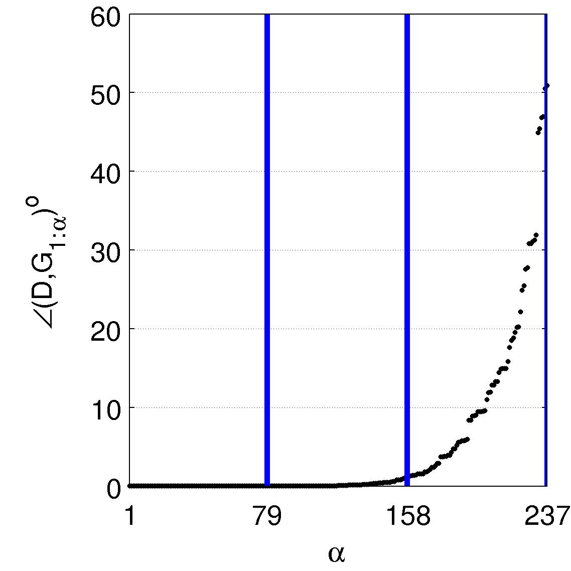
Figure 7.10: Angles (in degrees) between the spaces spanned by $\left(\widehat{G}_{\left\lvert{\mathcal{R}}\right\rvert,36}\right)_{1:\alpha}$ and the dictionary matrices $\widehat{D}_{{\mathcal{R}},36,1}$ (left) and $\widehat{D}_{{\mathcal{R}},36,2}$ (right), ${\mathcal{R}}=\text{Africa}$, $\alpha=1,\ldots,3N_{\left\lvert{\mathcal{R}}\right\rvert,L}$. Thick lines correspond to integer multiples of the Shannon number ${N_{\text{Africa},36}\approx 79}$.

Thanks to novel approaches to signal approximation, which we will discuss in the next section, the requirement that the dictionary elements form an orthogonal basis is less important than the property of mutual incoherence. Mutual incoherence in a dictionary means that the inner product (the angle, when elements are of unit norm) between pairs of elements is almost always very low. Figs. 7.11 and 7.12 numerically show that the two tree constructions on continental Africa have good incoherency properties: most dictionary element pairs are nearly orthogonal.

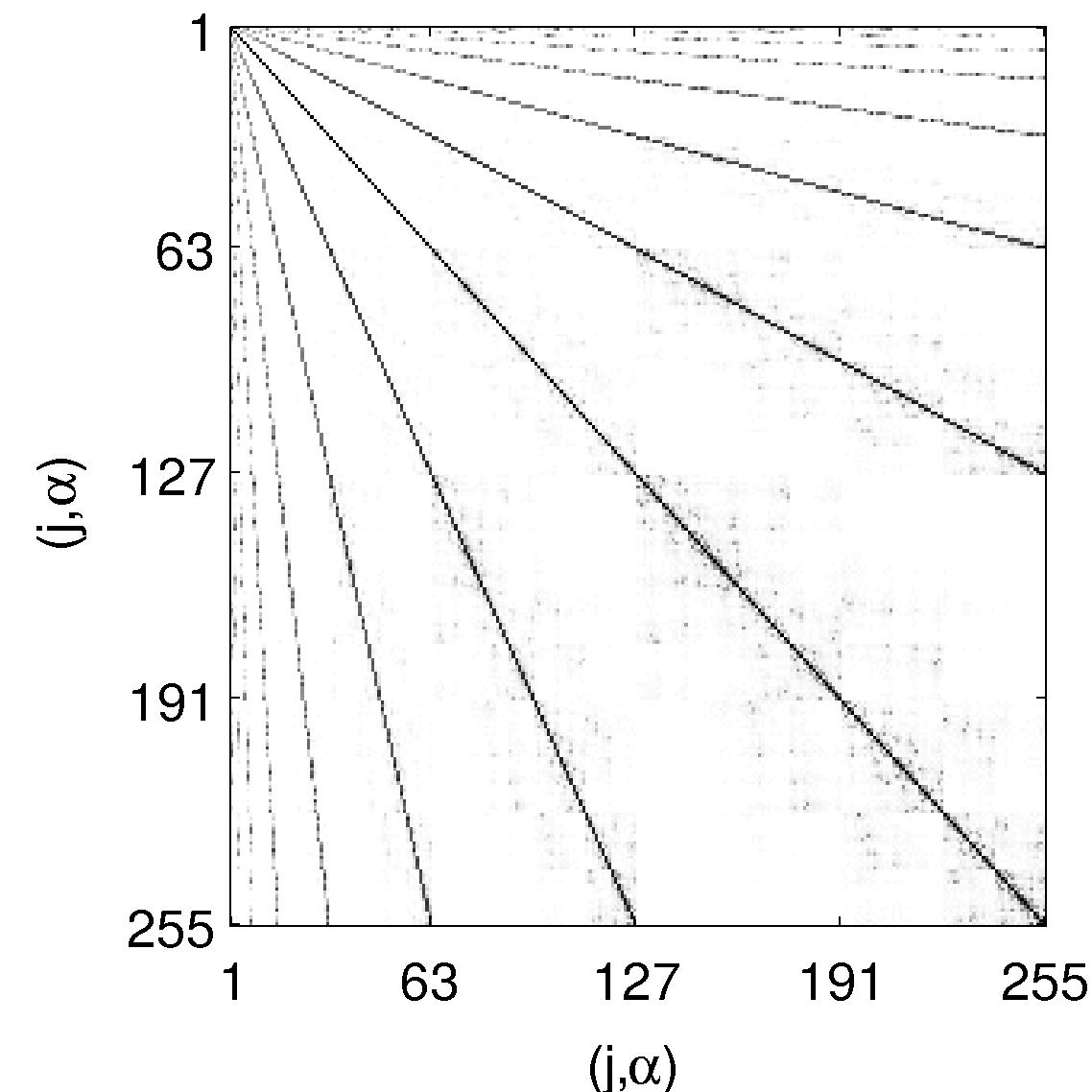
(a) ${\mathcal{D}}_{\text{Africa},36,1}$

(b) ${\mathcal{D}}_{\text{Africa},36,2}$

Figure 7.11: Magnitudes of pairwise inner products of dictionaries (a) ${\mathcal{D}}_{\text{Africa},36,1}$ and (b) ${\mathcal{D}}_{\text{Africa},36,2}$. In (b), as before, thick lines separate inner products between the 127 elements with $\alpha=1$ (top left) and $\alpha=2$ (bottom right), and their cross products. Values are between 0 (white) and 1 (black).

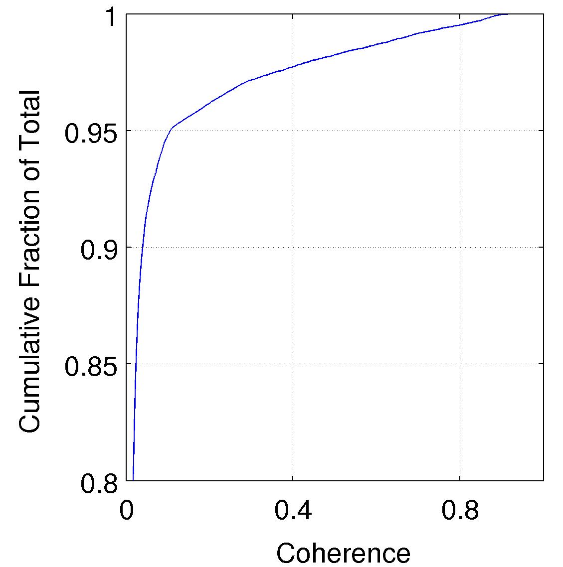
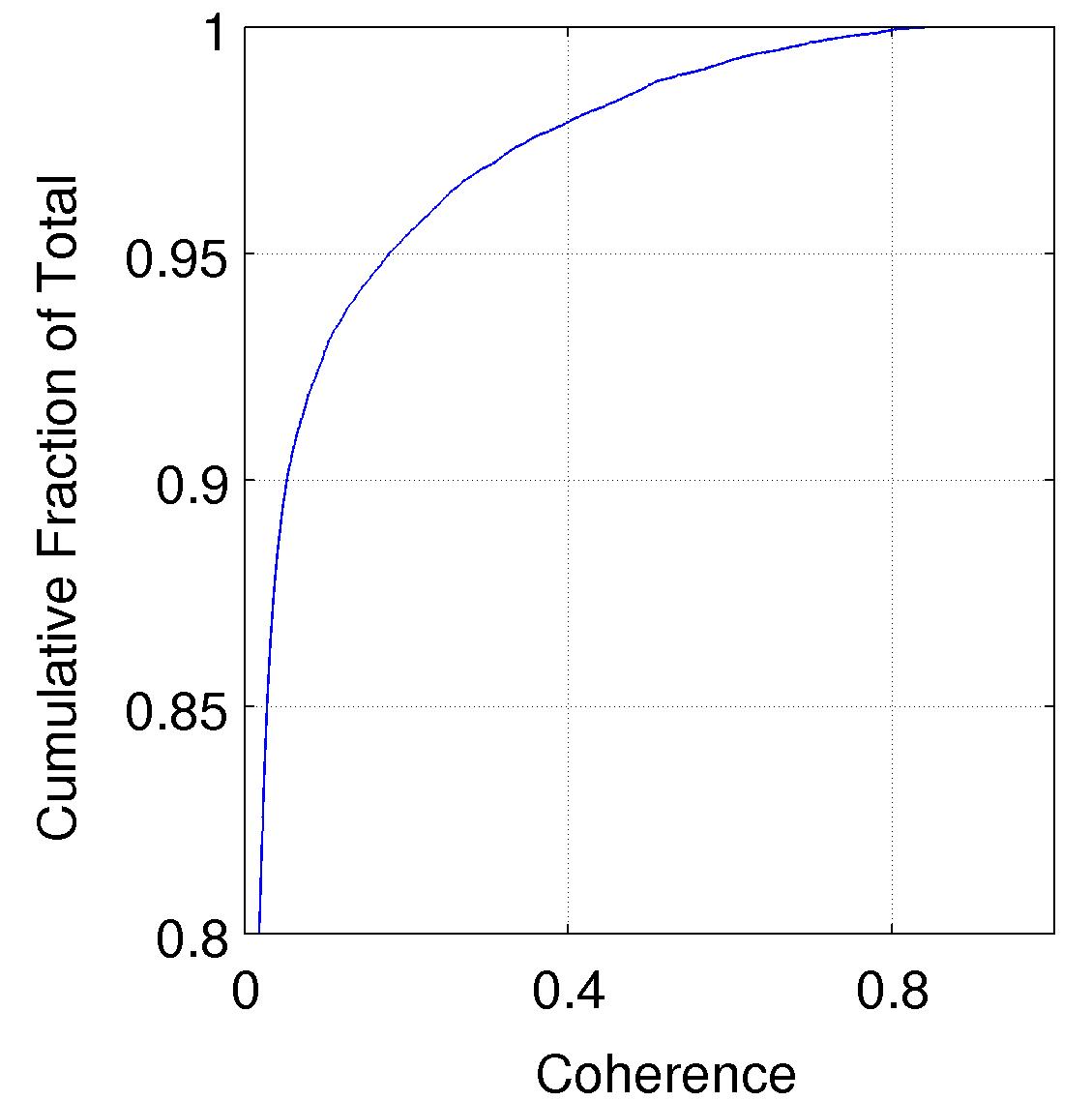
Figure 7.12: Empirical Cumulative Distribution Functions (CDFs) of pairwise inner product magnitudes for dictionaries ${\mathcal{D}}_{\text{Africa},36,1}$ (left) and ${\mathcal{D}}_{\text{Africa},36,1}$ (right). Note, in both cases, approximately $95\%$ of pairwise inner products have a value within $\pm 0.1$.

In Fig. 7.11(a), most pairwise inner products are nearly zero, with the exception of nodes and their ancestors, which share their parents’ regions. More specifically, as expected, dictionary elements ${(j,1)}$, ${(2j,1)}$, ${(2j+1,1)}$, ${(2(2j),1)}$, ${(2(2j)+1,1)}$, ${(2(2j+1),1)}$, ${(2(2j+1)+1,1),\ldots}$, tend to have large inner products, while those elements with non-overlapping borders do not. This exact property is also visible in the two diagonal submatrices of Fig. 7.11(b). In the off-diagonals, due to the orthonormality of the construction, elements of the form $(j,1)$ and $(j,2)$ are orthogonal. In contrast, due to the nature of the tree subdivision scheme, elements of the form $(2j,1)$ or $(2j+1,1)$ and $(j,2)$ have a large magnitude inner product. However, the number of connections between nodes and their ancestors is $O(n_{b}\,(2^{H}H))$, while the total number of pairwise inner products is $O((n_{b}2^{H})^{2})$; and for reasonably sized values of $L$ the ratio of ancestral connections to pairwise inner products grows small (see Fig. 7.12).

7.5 Solution Approaches for Linear Systems

As we will show in §7.6, the signal approximation problem on the sphere reduces to a linear problem of the form

$$y=A~{}x,$$ (7.20)

where $y\in{\mathbb{R}}^{m}$ are samples of a function on a region ${{\mathcal{R}}\subset S^{2}}$, $x\in{\mathbb{R}}^{n}$ are estimate coefficients in the given dictionary, and ${A\in{\mathbb{R}}^{m{\times}n}}$ represents a spatial discretization of the dictionary elements.

While the number of samples $m$ is usually larger than the number of dictionary elements, in practice, due to the nature of sampling and discretization (e.g., [100, Fig. 1b]), the rank $r$ of $A$ is significantly lower than $m$. There are several examples in the literature concerning spherical harmonics, for which (7.20) is invertible (that is, with $r=n\approx m$). For example, it can be shown via a Shannon-type theorem that when $x$ represents the spherical harmonic coefficients of a function with bandlimit $L$, $y$ represents its samples on a special semi-regular grid, and $A$ represents the discretization of the harmonics to the grid, the signal $x$ can be reconstructed exactly [35, Thm. 3]. In this case, the semi-regular grid consists of $m=4L^{2}$ points on the entire sphere $S^{2}$, and the number of harmonic coefficients (also the rank of $A$) is ${r=n=(L+1)^{2}}$. In the limit of large bandlimit $L$, the ratio of the samples to unknowns is $4$. As such, the sampling scheme presented in that paper is in a sense optimal in order of magnitude. Nevertheless, even there the rank is significantly lower than the sample number.

Under the assumption that $r<m$, we can write the compact Singular Value Decomposition (SVD) [49, Chapter 7] of $A$:

$$A=U_{+}\Sigma_{+}V_{+}^{*},\quad U_{+}^{*}U_{+}=I_{r{\times}r},\text{ and }V_{+}^{*}V_{+}=I_{r{\times}r}.$$ (7.21)

Here $U_{+}\in{\mathbb{R}}^{m{\times}r}$, $\Sigma_{+}\in{\mathbb{R}}^{r{\times}r}$ is a diagonal matrix of positive singular values, and $V_{+}\in{\mathbb{R}}^{n{\times}r}$. We can thus rewrite (7.20) as

$$\widehat{y}=\widehat{A}x,\quad\widehat{y}=U_{+}^{*}y,\text{ and }\widehat{A}=\Sigma_{+}V_{+}^{*},$$

where $\widehat{A}\in{\mathbb{R}}^{r{\times}n}$ and $r$ may be smaller than $n$.

We must therefore focus on (7.20) with all three possible cases: the overdetermined case $m>n$ (with rank $r=n$), the case $m=n$ (with rank $r=m=n$), and especially the underdetermined case $m>n$ (with rank $r=n$). We first quickly review the overdetermined case.

7.5.1 Overdetermined and Square Cases: $m\geq n$

When the system (7.20) is overdetermined, there many not be one exact solution $x$. However, in this case it is possible to minimize the sum of squared errors

$$x_{M}=\operatorname*{argmin}_{x\in{\mathbb{R}}^{n}}\left\lVert y-Ax\right\rVert_{2}^{2}.$$ (7.22)

Taking gradients with respect to vector $x$ and setting the resulting system equal to zero, we get the least squares solution

$$x_{M}=(A^{*}A)^{-1}A^{*}y.$$ (7.23)

Note that (7.22) arises from the Maximum Likelihood formulation of a statistical model in which the samples $y$ are observed as [10, Chapter 3]

$$y=Ax+n,$$

where $n\sim{\mathcal{N}}(0,\sigma^{2}I_{m{\times}m})$ is i.i.d Gaussian noise.

When $m=n=r$, (7.20) has exactly one solution. The matrix $A$ and its conjugate are invertible and, using the identity $(AB)^{-1}=B^{-1}A^{-1}$, (7.23) reduces to ${x_{M}=A^{-1}x}$, as expected.

7.5.2 Underdetermined Case: $m<n$

When the linear system $A$ has more unknowns than equations (or rank $r$), additional modeling or regularization is required. We discuss two possible statistical models on $x$, their limiting cases, and the resulting computational considerations.

Prior: $x$ distributed according to a Gaussian distribution

One possible way to model the underdetermined case is via a statistical model in which the coefficients of $x$ are generated i.i.d. with a zero-mean, fixed variance Gaussian distribution:

$$y|x =Ax+n,$$

$$n \sim{\mathcal{N}}(0,\sigma I_{m{\times}m}),\text{ and}$$

$$x \sim{\mathcal{N}}(0,\sigma_{s}I_{n{\times}n}).$$

The maximum a posteriori (MAP) estimate follows from Bayes’ rule:

$$\Pr(x|y) \propto\Pr(y|x)\Pr(x)$$

$$=\frac{1}{(2\pi)^{(m+n)/2}\sigma^{m/2}\sigma_{s}^{n/2}}\exp\left\{-\left(\left\lVert y-Ax\right\rVert^{2}_{2}/2\sigma^{2}+\left\lVert x\right\rVert^{2}_{2}/2\sigma_{s}^{2}\right)\right\}.$$

When $\sigma$ and $\sigma_{s}$ are fixed, maximizing $\Pr(x|y)$ is equivalent to minimizing its negative logarithm. The MAP problem in this case becomes

$$x_{N}=\operatorname*{argmin}_{x\in{\mathbb{R}}^{n}}\left\lVert y-Ax\right\rVert_{2}^{2}+\gamma^{2}\left\lVert x\right\rVert_{2}^{2},$$ (7.24)

where ${\gamma=\sigma/\sigma_{s}}$.

Simple calculus again provides the solution, also known as the Tikhonov regularized solution to (7.24):

$$x_{N}=(A^{*}A+\gamma^{2}I)^{-1}A^{*}y.$$ (7.25)

When the model noise power $\sigma$ grows small with respect to the signal power $\sigma_{s}$, the regularization term $\gamma$ goes to zero. In this limiting case, we can write the limiting solution as [49, pp 421-422]

$$x_{MP}=\lim_{\gamma^{2}\to 0}(A^{*}A+\gamma^{2}I)^{-1}A^{*}y=A^{\dagger}y,$$ (7.26)

where $A^{\dagger}$ is the Moore-Penrose generalized inverse of $A$. For overdetermined and exactly determined systems, $A^{*}A$ has a well defined inverse and $A^{\dagger}$ coincides with the matrix in (7.23). For underdetermined systems, the matrix $A^{\dagger}$ is still well defined, and is given by

$$A^{\dagger}=U_{+}\Sigma_{+}^{-1}V_{+}^{*},$$

where $U,\Sigma,V$ are given by the SVD as in (7.21). Note that $x_{MP}$ also solves the convex, quadratic optimization problem

$$x_{MP}=\operatorname*{argmin}_{x\in{\mathbb{R}}^{m}}\left\lVert x\right\rVert_{2}^{2}\text{ subject to }y=Ax.$$

The Tikhonov and Moore-Penrose solutions (7.24) and (7.26) are a common approach to solving underdetermined inverse problems in the Geosciences literature (see e.g., [113]). However, depending on the dictionary used for the representation of $x$ the Gaussian prior may not be an ideal one; as it encourages all of the coefficients to be nonzero.

One of the major underlying foundations of this work includes recent results in representation theory, which have shown that overcomplete (redundant) multiscale frames and dictionaries with certain incoherency properties can provide stable and noise-robust estimates to ill-posed inversion problems. The basic requirement in the estimation stage is that the solution is as “simple” as possible: most of the coefficients in of the solution $x$ are zero; $x$ is sparse. We discuss this next.

Prior: $x$ distributed according to a Laplace distribution

It is well known in the statistics community (and, most recently, in the Compressive Sensing literature), that applying a super Gaussian prior $\Pr(x)$ induces MAP solutions that have many zero components and a few large magnitude ones. The zero-mean Laplace distribution is one such particularly convenient distribution. We model each component of $x$, $x_{i}$ as i.i.d. Laplace distributed:

$$\Pr(x)=\prod_{i=1}^{n}\frac{1}{2b}\exp(-\left\lvert x_{i}\right\rvert/b)=\frac{1}{(2b)^{n}}\exp(-\left\lVert x\right\rVert_{1}/b).$$

In a manner identical to that of the previous section, for fixed noise power $\sigma^{2}$ and signal scale $b>0$, the MAP problem can be reduced to

$$x_{L}=\operatorname*{argmin}_{x\in{\mathbb{R}}^{n}}\left\lVert y-Ax\right\rVert_{2}^{2}+\eta\left\lVert x\right\rVert_{1},$$ (7.27)

where $\eta=2\sigma/b$. For any $\eta>0$, there is a $t>0$ such that the following problem is identical:

$$\operatorname*{argmin}_{x\in{\mathbb{R}}^{n}}\left\lVert y-Ax\right\rVert_{2}^{2}\text{ subject to }\left\lVert x\right\rVert_{1}\leq t,$$ (7.28)

where for a given $\eta$, there exists a $t(\eta)>0$ such that (7.28) gives a solution identical to (7.27), and $t(\eta)$ decreases monotonically with $\eta$. Furthermore, for any given $t$ to (7.28), an $\eta$ can be found for (7.27) that provides the identical solution [67, §12.4.2]; this result essentially follows from the method of Lagrange multipliers. In other words, the two convex problems are completely equivalent. They are also equivalent to the popularly studied Compressive Sensing problem

$$\operatorname*{argmin}_{x\in{\mathbb{R}}^{n}}\left\lVert x\right\rVert_{1}\text{ subject to }\left\lVert y-Ax\right\rVert_{2}^{2}\leq\epsilon,$$

where $\epsilon$ grows monotonically in $\eta$ and/or $t^{-1}$.

Fast and robust solvers for the convex quadratic optimization problems (7.27) and (7.28) have been the subject of study for many years. For our calculations we use the LASSO solver (see, e.g., [107]). LASSO is an iterative solution method that provides the full solution paths to (7.28). It is computationally efficient for small- to medium- scale linear systems. For systems with more than tens of thousands of unknowns, there are a variety of other techniques for the solution of (7.28) that are much more computationally tractable, though possibly less accurate (see, e.g., [30] and [67, §12.4, §12.5]).

Debiasing the $\ell_{1}$ solution

An alternative approach to finding a sparse solution of (7.20) is to attempt to minimize the problem

$$\min_{x\in{\mathbb{R}}^{n}}\left\lVert y-Ax\right\rVert\text{ subject to }\left\lVert x\right\rVert_{0}\leq\kappa,$$ (7.29)

where $\left\lVert x\right\rVert_{0}=\left\lvert\text{supp}\left(x\right)\right\rvert$ and ${\text{supp}\left(x\right)=\left\{i:x_{i}\neq 0\right\}}$. That is, find the best matching data to the model where the number of nonzero coefficients of the model is bounded by $\kappa$. Unfortunately, this combinatorial problem is nonconvex and therefore usually intractable. In some cases, it can be shown that the solution is equivalent to the $\ell_{1}$ problem (7.28), when the matrix $A$ fulfills one of a number of special properties, e.g., the Restricted Isometry Property (RIP) or Null Space Property (NSP). This result is, in fact, a celebrated equivalence result in Compressive Sensing [17, 34]. Unfortunately, for physical discretization matrices $A$, the RIP and its equivalents are difficult to check [28, 55].

In practice, problem (7.29) can be reduced into two parts:

1. Estimate the support of $x$, ${\mathcal{S}}=\text{supp}\left(x\right)$, such that $\left\lvert{\mathcal{S}}\right\rvert<r$.

2. Solve the overdetermined system (7.22) via (7.23) on the reduced set $\text{supp}\left(x\right)$ by keeping only the columns of $A$ associated with $\text{supp}\left(x\right)$, $A_{\text{supp}\left(x\right)}$, when solving the least squares problem.

A tractable solution to the first part is to use the output of the $\ell_{1}$ (LASSO) estimator:

$${\mathcal{S}}=\text{supp}\left(x\right)=\text{supp}\left(x_{L}\right).$$

The final estimate is the vector $x_{D}$ where

$$x^{\prime}_{D} =\operatorname*{argmin}_{x^{\prime}\in{\mathbb{R}}^{\left\lvert{\mathcal{S}}\right\rvert}}\left\lVert y-A_{{\mathcal{S}}}x^{\prime}\right\rVert_{2}^{2},\text{ and }$$ (7.30)

$$x_{D,i} =x^{\prime}_{D,i}\delta_{i\in{\mathcal{S}}},\quad i=1,\ldots,n.$$

This alternative solution is also sometimes called the debiased $\ell_{1}$ solution, because after the $\ell_{1}$ minimization step, the bias of the $\ell_{1}$ penalty is removed via least squares on the estimated support.

As we will show in the next section, this final combination of support estimate based on a sparsity-inducing prior, followed by the solution to an overcomplete least squares problem on this support set, allows for improvements in signal approximation over currently standard techniques in geophysics.

7.6 Signal Approximation Models for Subsets of the Sphere $S^{2}$

We now turn to the problem of estimating a signal from noisy and/or incomplete observations on a subset ${\mathcal{R}}$ of the sphere. Following the notation of [90], suppose we observe data (samples of some function $f$) on a set of points within the region ${\mathcal{R}}$, consisting of signal $s$ plus noise $n$. We are interested in estimating the signal within ${\mathcal{R}}$ from these samples.

While in practice, most signals of interest in geophysics are not bandlimited, this assumption allows us to perform estimates, and can be thought of as a regularization of the signal, similar in nature to assumptions of a maximum frequencies in audio analysis. Furthermore, as in 1D signal processing, constraints on physical sampling and high frequency noise always reduce the maximum determinable frequency. See, for example, a noise analysis for satellite observations in the GRACE mission [110, Fig. 1], and the effects of noise on power spectral estimation for the CMB dataset [27, Fig. 12].

Let ${{\mathcal{X}}=\left\{x_{i}\right\}_{i=1}^{m},x_{i}\in{\mathcal{R}}}$ be a set of points on which data $f$ is observed, and let the corresponding observations be $\left\{f_{i}=f(x_{i})\right\}_{i=1}^{m}$, which we denote with the vector ${\tilde{f}}$. Then via the harmonic expansion (7.6), we can write

$$f_{i}=\sum_{l=0}^{L}\sum_{m=-l}^{l}\widehat{s}_{lm}Y_{lm}(\theta_{i},\phi_{i})+\nu_{i},$$ (7.31)

where the $\widehat{s}_{lm}$ are the harmonic expansion coefficients of the signal $s$ and $\nu_{i}=\nu(x_{i})$ is a realization of the noise. We will also denote by ${\widetilde{\nu}}$ the vector of samples of the noise process. Let $Y$ be the $\left\lvert{\mathcal{X}}\right\rvert{\times}(L+1)^{2}$ harmonic sensing matrix, with

$${Y_{i,lm}=Y_{lm}(\theta_{i},\phi_{i})}\text{ for }i=1,\ldots,\left\lvert{\mathcal{X}}\right\rvert,\text{ and }(l,m)\in\Omega.$$

Then we can rewrite (7.31) as

$${\tilde{f}}=Y\widehat{s}+{\widetilde{\nu}}.$$ (7.32)

By restricting the bandlimit to $L$, we restrict the function $s$ to lie in $L^{2}_{\Omega}(S^{2})$. Moreover, we are only interested in estimating $s$ on ${\mathcal{R}}\subset S^{2}$.

The Slepian functions are another basis for $L^{2}_{\Omega}(S^{2})$, in which the functions are ordered in terms of their concentration on ${\mathcal{R}}$. As such, we may rewrite the samples via their Slepian expansion:

$$f_{i}=\sum_{\alpha=1}^{n}\widetilde{s}_{\alpha}g_{\alpha}(\theta_{i},\phi_{i})+\nu_{i}$$ (7.33)

where now the $\widetilde{s}_{\alpha}$ are the Slepian expansion coefficients, and we are free to constrain $n$ from $1$ through $(L+1)^{2}$. By setting $n$ to $N_{\left\lvert{\mathcal{R}}\right\rvert,L}$, we concentrate the estimate to ${\mathcal{R}}$, while choosing $n=(L+1)^{2}$ leads to a representation equivalent to (7.31).

Using the harmonic expansion of the Slepian functions, we rewrite (7.33) via the spherical harmonics:

$$f_{i}=\sum_{\alpha=1}^{n}\widetilde{s}_{\alpha}\sum_{l=0}^{L}\sum_{m=-l}^{l}\widehat{g}_{\alpha,lm}Y_{lm}(\theta_{i},\phi_{i})+\nu_{i},$$ (7.34)

and, using the terminology $\widehat{G}$ of §7.4 to denote the harmonic expansion matrix of the Slepian functions, and the “colon” notation to denote restrictions of matrices and vectors to specific index subsets, we can rewrite (7.33) in matrix notation:

$${\tilde{f}}=Y\widehat{G}_{1:n}\widetilde{s}_{S,{1:n}}+{\widetilde{\nu}}.$$ (7.35)

As just described, by setting $n<(L+1)^{2}$ this model assumes that all but the first $n$ of the Slepian coefficients $\widetilde{s}_{S}$ are zero.

Finally, using the Tree dictionary construction of §7.3 and the notation of §7.4, for a given dictionary ${\mathcal{D}}_{{\mathcal{R}},L,n_{b}}$ we can model the signal with the linear model

$$f_{i}=\sum_{\alpha=1}^{n_{b}}\sum_{j=1}^{2^{H+1}-1}\widetilde{s}_{T,(j,\alpha)}d^{(j,\alpha)}_{{\mathcal{R}},L,n_{b}}(\theta_{i},\phi_{i})+\nu_{i}.$$ (7.36)

Writing the dictionary elements via their harmonic expansions, the matrix formulation of (7.36) becomes

$${\tilde{f}}=Y\widehat{D}_{{\mathcal{R}},L,n_{b}}\widetilde{s}_{T}+{\widetilde{\nu}}.$$ (7.37)

As we will see next, this alternative way of describing bandlimited functions on ${\mathcal{R}}$ has a number of advantages.

7.6.1 Regularized Inversion and Numerical Experiments

In practice, the sensing matrix $Y$ is highly rank deficient: depending on the sensing grid points ${\mathcal{X}}$, its rank $r$ tends to be significantly smaller than the maximum possible value $n$, $\dim L^{2}_{\Omega}(S^{2})=(L+1)^{2}$. As such, the estimation of $s$ via direct inversion of (7.32) is ill conditioned: it must be regularized.

As discussed in §7.5, the most common form of regularization is via the Moore-Penrose pseudoinverse: (7.23) for overdetermined systems or (7.26) for underdetermined ones. Following the discussion of §7.2.3 and the statistical analyses in [90, §3] and [91, §7], the “classically” optimal way to estimate $\widetilde{s}$ is by restricting the reconstruction to be concentrated within ${\mathcal{R}}$: that is, first by choosing a small $n$ in (7.35), such that $n<r$, and then applying (7.23) to estimate $\widetilde{s}_{S}$. In practice, we can consider $n$ ranging from $1$ to $N_{\left\lvert R\right\rvert,L}$ because the Shannon number is less than rank $r$. We will call this first estimation method Slepian Truncated Least Squares (STLS).

We now propose, first, a simple alternative approach: assume sparsity of $\widetilde{s}$ (i.e., with respect to the Slepian basis). As the Slepian basis was initially constructed to promote sparsity in the representation of bandlimited functions concentrated on ${\mathcal{R}}$ [§3.1.2][90], we expect that this assumption should lead to estimates that are equivalent to STLS, if not better. The basic idea is to let $n=(L+1)^{2}$ in (7.35), and use the solution method (7.30) with sparsity penalties $\eta_{1}\geq\eta_{2}\geq\cdots$ sufficiently large that only a few nonzero coefficients are found in the support. We consider a range of values $\eta$ from a maximum $\overline{\eta}$ that induces only one nonzero coefficient, to a minimum $\underline{\eta}$ that induces $N_{\left\lvert{\mathcal{R}}\right\rvert,L}$. We call this estimation method Slepian $\ell_{1}$ + Debias (SL1D). Though in this case we do not explicitly require the estimate to be well concentrated in ${\mathcal{R}}$ via choice of basis functions, by minimizing the squared error between sample values on ${\mathcal{X}}\subset{\mathcal{R}}$ we expect that most of estimated support will be within the first Slepian functions.

With the Tree construction of §7.3, we have a new dictionary of elements that are both concentrated in ${\mathcal{R}}$, bandlimited, and multiscale. As such, these dictionaries are excellent candidates for estimation via the $\ell_{1}$+ Debias technique (7.30). This method is similar to the previous one: apply (7.30) to the model (7.37), choosing a range of $\ell_{1}$ penalties $\eta$ that lead to between $1$ and $N_{\left\lvert{\mathcal{R}}\right\rvert,L}$ dictionary elements in the support of $\widetilde{x}_{T}$. We call this the Slepian Tree $\ell_{1}$ Debias (STL1D) method.

The experiments below numerically show that the two new estimation (inversion) methods SL1D and STL1D provide improved performance over the classic STLS, in terms of average reconstruction error over the domain of interest ${\mathcal{R}}$ using a small number of coefficients, for several important types of bandlimited signals. Furthermore, as expected the multiscale and spatially concentrated dictionary elements of the Tree construction provide improved estimation performance when the signal is “red”, i.e., when it contains more energy in the lower harmonic components.

Bandpass Filtered POMME Model

Fig. 7.13 shows a bandpass filtered version of the radial component of Earth’s crustal magnetic field, which we will call $p(\theta,\phi)$: a preprocessed version of the output of the POMME model [70]. The signal $p$ has been:

1. Bandpassed between $l_{\text{min}}=9$ and $l_{\text{max}}=36$.

2. Spatially tapered (multiplied) by the first Slepian function bandlimited to ${L_{t}=18}$ and concentrated within Africa.

3. Low-pass filtered to have maximum frequency $L=36$ via direct projection onto the first $(L+1)^{2}$ spherical harmonics using standard Riemannian sum-integral approximations [90, Eq. 80], i.e., direct inversion.

It can be shown [112, §2] that the harmonics of the tapered signal, at degree $l$, receive contributions from the original coefficients in the range from $\left\lvert l-L_{t}\right\rvert$ to $l+L_{t}$. As a result, only the first $l_{\text{max}}-L_{t}$ degree coefficients are reliable estimates of the original signal’s harmonics.

Samples of $p$ are given via the forward model (7.31) (with ${\widetilde{\nu}}=0$), from the low-pass filtered “ground truth” signal $\widetilde{p}$, on the intersection of the African continent ${\mathcal{R}}$ with the grid

$${\mathcal{X}}^{*}=\left\{(k_{\theta}\Delta,k_{\phi}\Delta),\Delta=0.25^{o},k_{\theta}=\pm 0,\pm 1,\ldots,k_{\phi}=\pm 0,\pm 1,\ldots\right\}$$

We denote this reduced set ${\mathcal{X}}$; it contains $\left\lvert{\mathcal{X}}\right\rvert=40250$ points. For $L=36$, as before, the Shannon number of Africa is $N_{\text{Africa},36}\approx 79$, the dimension of the bandlimited space is $\dim L^{2}_{\Omega}(S^{2})=(L+1)^{2}=1639$, and the rank of the discretization matrix in (7.31), $Y_{1:(L+1)^{2}}$, is ${r=528}\ll 1639$.

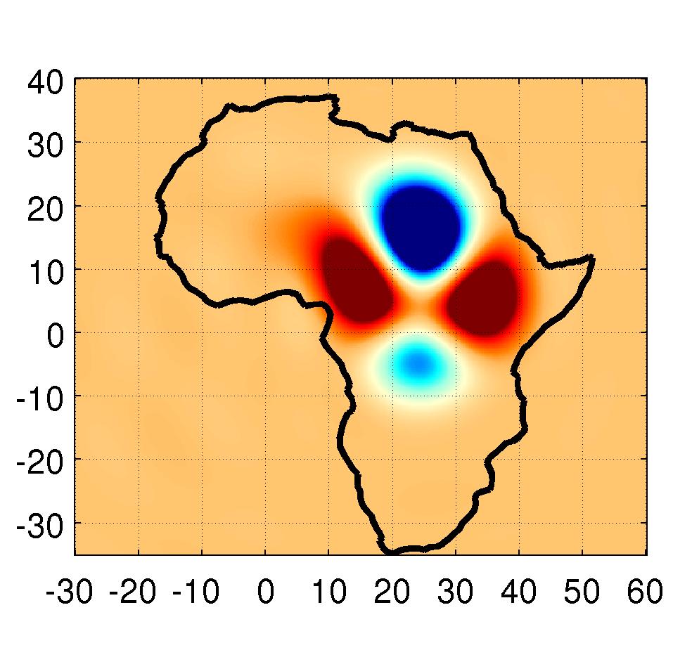
Figure 7.13: The tapered and preprocessed “ground truth” POMME-4 signal $p$, sampled on the regular grid ${\mathcal{X}}^{*}$ around Africa. Red colors are high magnitude positive values, blue are high magnitude negative values.

Figs. 7.14, 7.15, and 7.16 show intermediate results in the estimation of $p$ via the three methods: STLS, SL1D, and STL1D, respectively. Specifically, they show the absolute error between the original sampled signal ${\tilde{p}}$, and the expansion via (7.6) of the three estimates. In Fig. 7.14, the number of nonzero coefficients in the estimate is determined by the Slepian truncation number $n$, while in Figs. 7.15 and 7.16, the number of nonzero coefficients are indirectly determined by the parameter $\eta$ after the support estimation stage, as per our earlier discussion. As such, the number of nonzero components do not always match that of Fig. 7.14; instead nearby values are used when found.

(a) $e_{10}$

(b) $e_{20}$

(c) $e_{30}$

(d) $e_{40}$

(e) $e_{50}$

(f) $e_{60}$

Figure 7.14: Residual errors of the Slepian Truncated Least Squares Reconstruction of POMME-4 data, using the $L=36$ basis concentrated on Africa. Labels above describe the number of nonzero entries in the reconstructed estimate. Absolute error values range between 0 (white) to 50 (black) and above (thresholded black).

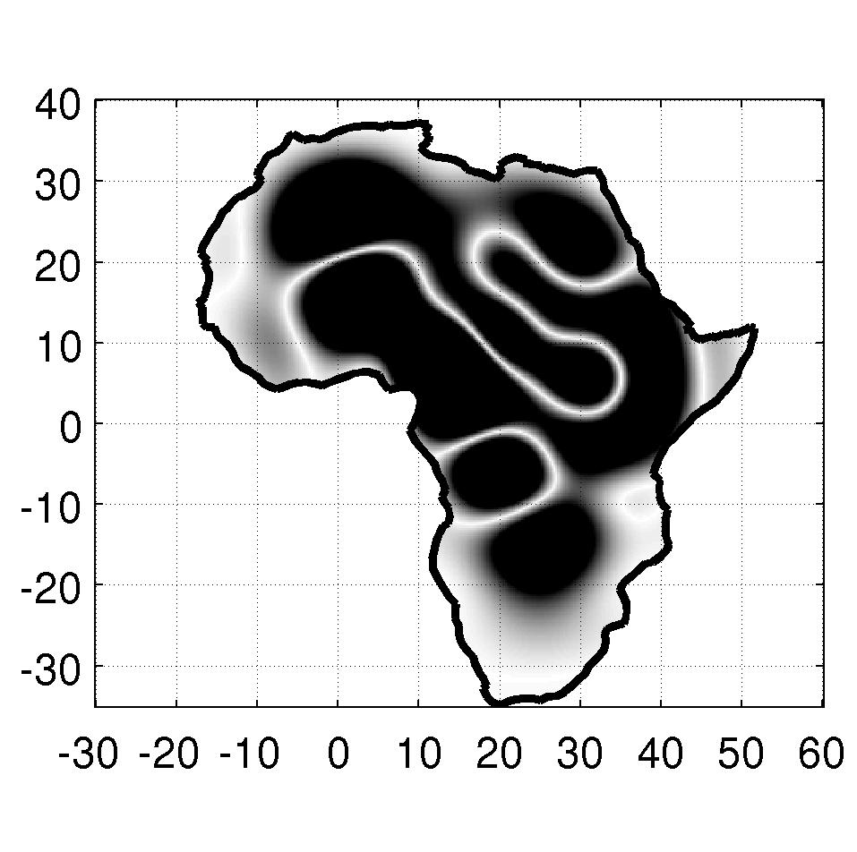
(a) $e_{10}$

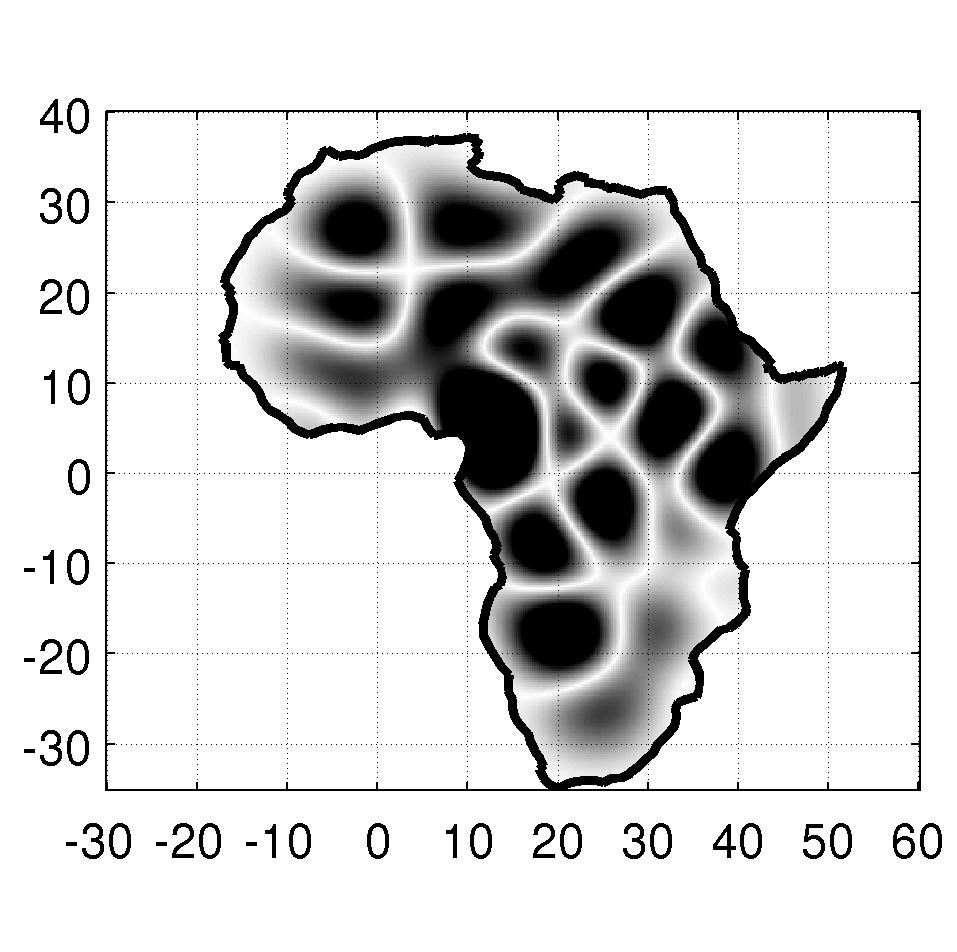
(b) $e_{20}$

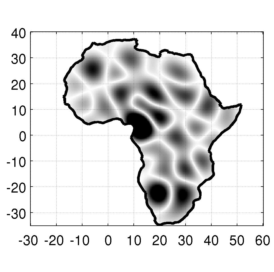
(c) $e_{30}$

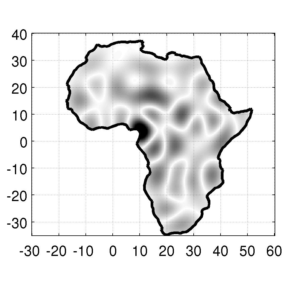
(d) $e_{42}$

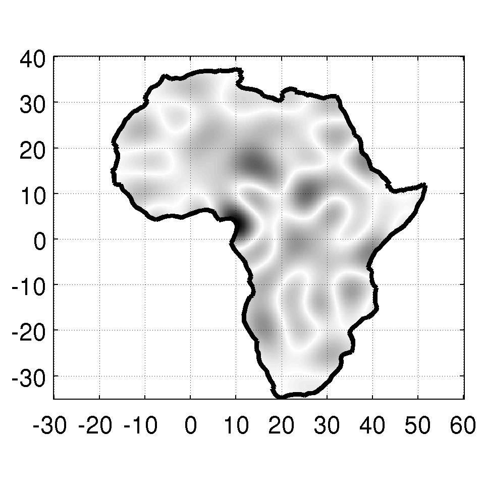
(e) $e_{50}$

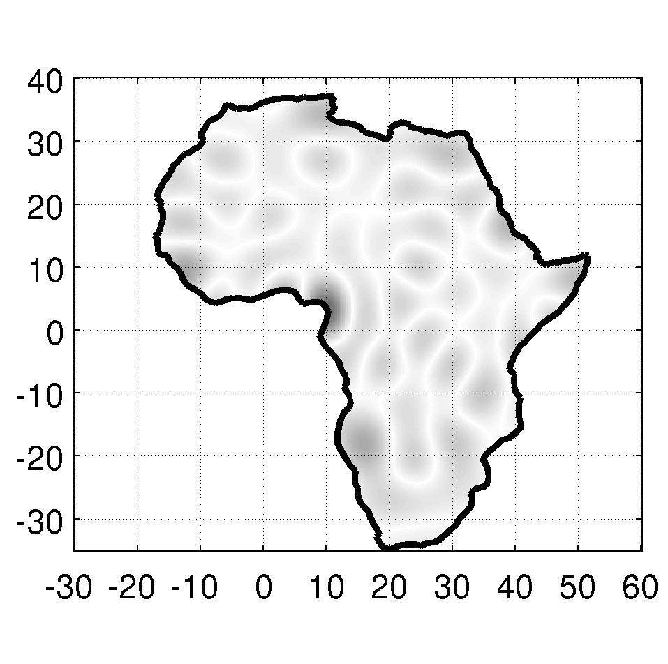
(f) $e_{61}$

Figure 7.15: Residual errors of the Slepian $\ell_{1}$ + Debias Reconstruction of POMME-4 data, using the $L=36$ basis concentrated on Africa. Labels above describe the number of nonzero entries in the reconstructed estimate. Absolute error values range between 0 (white) to 50 (black) and above (thresholded black).

(a) $e_{9}$

(b) $e_{20}$

(c) $e_{31}$

(d) $e_{40}$

(e) $e_{50}$

(f) $e_{62}$

Figure 7.16: Residual errors of the Slepian Tree $\ell_{1}$ Debias Reconstruction of POMME-4 data, using dictionary ${\mathcal{D}}_{\text{Africa},36,1}$. Labels above describe the number of nonzero entries in the reconstructed estimate. Absolute error values range between 0 (white) to 50 (black) and above (thresholded black).

As the dictionary elements given by the Tree construction are localized in both scale and location, we can graphically show which elements are “turned on” through the solution path, as more and more elements in the support are chosen to be nonzero. Fig. 7.17 shows the supporting regions $\left\{{\mathcal{R}}^{(j,\alpha)}\right\}$ of dictionary ${\mathcal{D}}_{\text{Africa},36,1}$ associated the solutions given in the corresponding panels of Fig. 7.16. Clearly, larger scale dictionary elements are chosen first; these reduce the residual error the most. As more and more dictionary elements are added during the $\ell_{1}$ based inversion process, finer and finer details are included in the reconstruction.

(a) ${\mathcal{S}}_{9}$

(b) ${\mathcal{S}}_{20}$

(c) ${\mathcal{S}}_{31}$

(d) ${\mathcal{S}}_{40}$

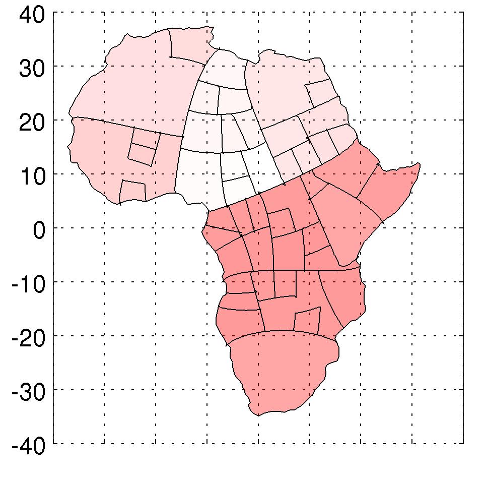
(e) ${\mathcal{S}}_{50}$

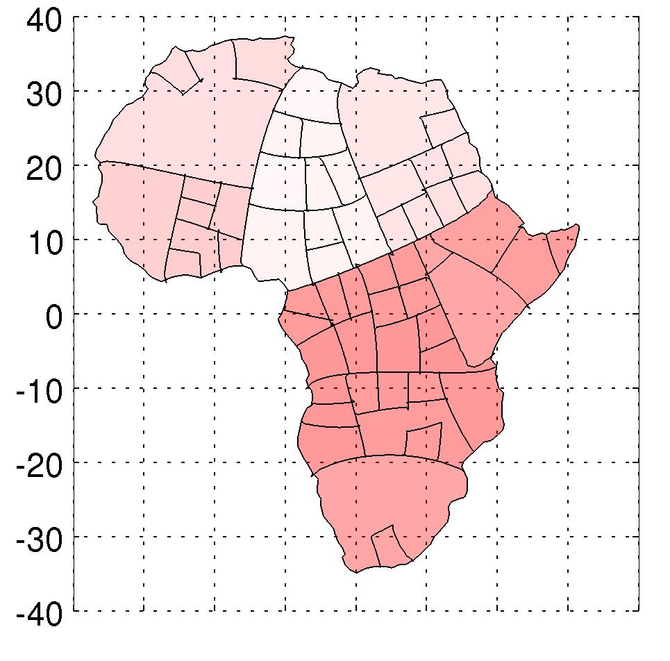
(f) ${\mathcal{S}}_{62}$

Figure 7.17: Support sets as estimated during the Slepian Tree $\ell_{1}$ Debias Reconstruction of POMME-4. The dictionary used was ${\mathcal{D}}_{\text{Africa},36,1}$. These panes are associated with their corresponding panes in Fig. 7.16.

Fig. 7.18 compares, on a logarithmic scale, the spatial residual errors (sum of squared differences) between the three estimates, as a function of the number of nonzero components allowed. Clearly, when a small number of nonzero components is allowed, the sparsity-based estimators outperform the standard Slepian truncation-based inversion.

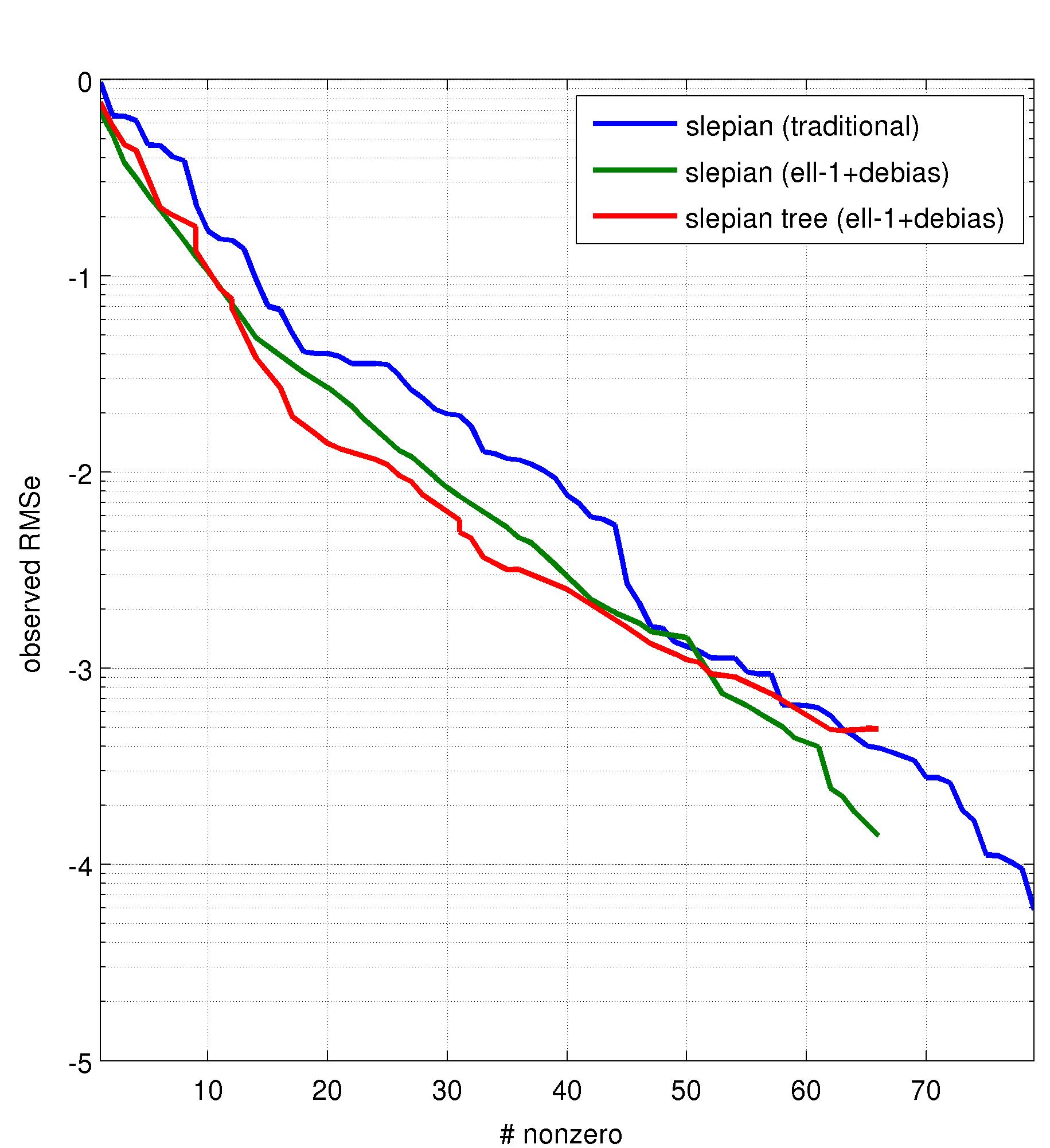
Figure 7.18: Normalized residual error during reconstruction of POMME-4 data vector ${\tilde{p}}$. Values are proportional to the sum of squared differences between ${\tilde{p}}$ and the spatial expansions of its estimates via STLS, SL1D, and STL1D, on the grid ${\mathcal{X}}$. The x-axis denotes the number of nonzero components allowed. The y-axis is on a base-10 logarithmic (dB) scale.

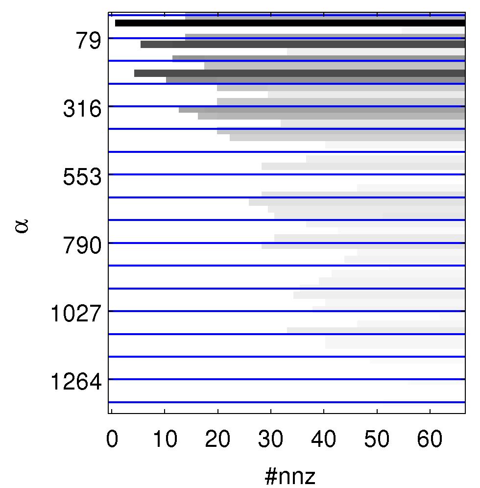
Figure 7.19: Solution paths for the SL1D and STL1D estimators on the POMME-4 data ${\tilde{p}}$. On the left, the solution path (coefficient magnitudes vs. support size) for the SL1D estimator. Blue horizontal lines represent multiples of the Shannon number $N_{\text{Africa},36}\approx 79$. On the right, the solution path for the STL1D estimator with dictionary ${\mathcal{D}}_{\text{Africa},36,1}$.

To study the consistency of the $\ell_{1}$-based SL1D and STL1D estimators, and as a measure of how closely the SL1D method matches the classical truncation strategy, we plot the solution paths of these two estimators. Fig. 7.19 shows that while lower order (better-concentrated in ${\mathcal{R}}$) Slepian functions were chosen early on, when $n$ was small. However, as more and more nonzero indices were allowed, less well concentrated Slepian functions, with lower magnitudes, were included in the solution, probably as small “tweaks” to the estimate near the edges of the region. Once a Slepian function was included into the solution, its magnitude did not change much throughout the solution path (as other elements were added).

In contrast to the behavior of SL1D, the Slepian Tree solution chose particular elements localized to the main features of the signal, not simply elements that are well concentrated in all of Africa on a large scale. In addition, as the size of the support was allowed to increase, the magnitudes of some coefficients were decreased as new elements were added. This supports the general statement that multiscale dictionaries, when combined with sparsity-inducing reconstruction techniques, “fit” the support to the nature of the data. Figs. 7.18 and 7.19 thus help to clarify the behavior of the STL1D estimator.

White and Pink Noise

As a second experiment, we generated multiple observations of either pink or white noise fields, with a bandlimit of $L=36$, on the sphere $S^{2}$, via randomization in the spherical harmonic representation of $L^{2}_{\Omega}(S^{2})$. We then sampled these on ${\mathcal{X}}$ to and attempted to reconstruct them only in Africa, as in the previous example.

A random field $r$ with spectral slope $\beta$, up to degree $L$, is defined as having the harmonic coefficients

$$\widehat{r}_{lm} =l^{\beta/2}N_{l}^{-1}n_{lm}\quad(l,m)\in\Omega,$$ (7.38)

$$\text{where }n_{lm} \operatorname*{\sim}^{\text{i.i.d.}}{\mathcal{N}}(0,1)\quad(l,m)\in\Omega,$$

$$\text{and }N_{l} =(2l+1)^{-1}\textstyle{\sqrt{\sum_{m=-l}^{l}n_{lm}^{2}}}.$$

For a white noise process, with equal signal power across its spectrum, $\beta=0$. Most spatial processes in geophysics, however, have some $\beta<0$; their power drops off with degree $l$. Fields with $\beta$ near $-2$ are considered to be “pink”, while fields with $\beta$ near $-4$ are “red”. The more red a noise process, the higher its spatial correlation, the less “random” it looks. The earth’s geopotential field, for example, is modeled as having ${\beta=-4.036}$. In our experiments, we use $\beta=0$ to generate white noise processes and $\beta=-2$ for pink.

For each of $T=200$ iterations, we generated both pink and white noise fields $r$ (bandlimited to $L=36$) and sampled them on ${\mathcal{X}}$ (the grid over the African continent) to get the vectors ${\tilde{r}}$. As before, the discretization matrix $Y$ is of rank $r=528$ so direct inversion is impossible. We again performed reconstruction via the three methods STLS, SL1D, and STL1D. As in Fig. 7.18, for each of the iterations we calculated the normalized residual: the sum of squared differences between the estimates, as expanded on ${\mathcal{X}}$, and the original samples, normalized by the sum of squares $\left\lVert{\tilde{r}}\right\rVert_{2}^{2}$.

Figs. 7.20 and 7.21 show the mean normalized error over the $T$ iterations for white and pink noise, respectively. For white noise, the ability to use any of the Slepian functions clearly provides an advantage for the SL1D algorithm. In contrast, for pink noise the spatial localization of the dictionary elements and the smaller size of the dictionary give an edge to the Tree-based estimator. Clearly, however, both estimators lead to lower normalized observation error on average, as compared with the classically optimal Slepian truncation method STLS.

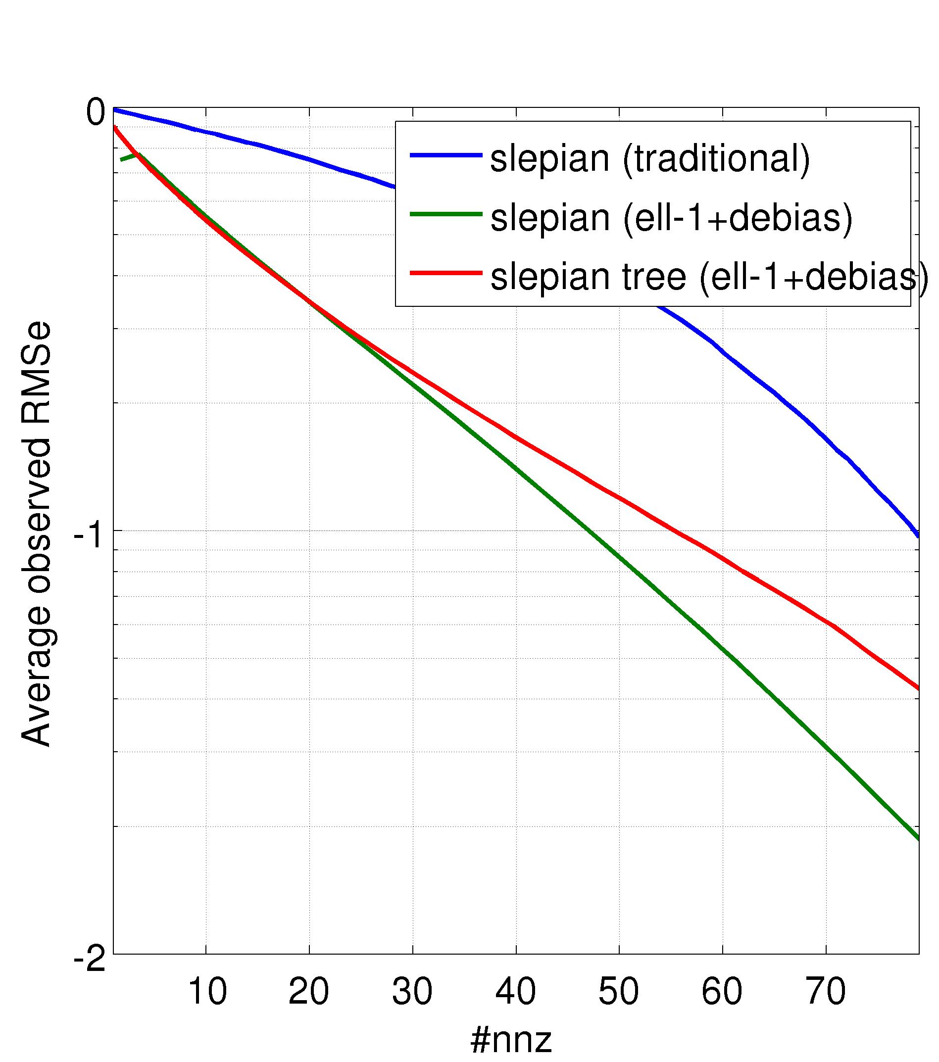
Figure 7.20: White noise ($\beta=0$) average reconstruction error, normalized by signal power within each iteration, on a base-10 log scale. Average taken over $T=200$ iterations. X-axis represents the number of nonzero elements allowed in the support. The Tree dictionary is ${\mathcal{D}}_{\text{Africa},36,1}$.

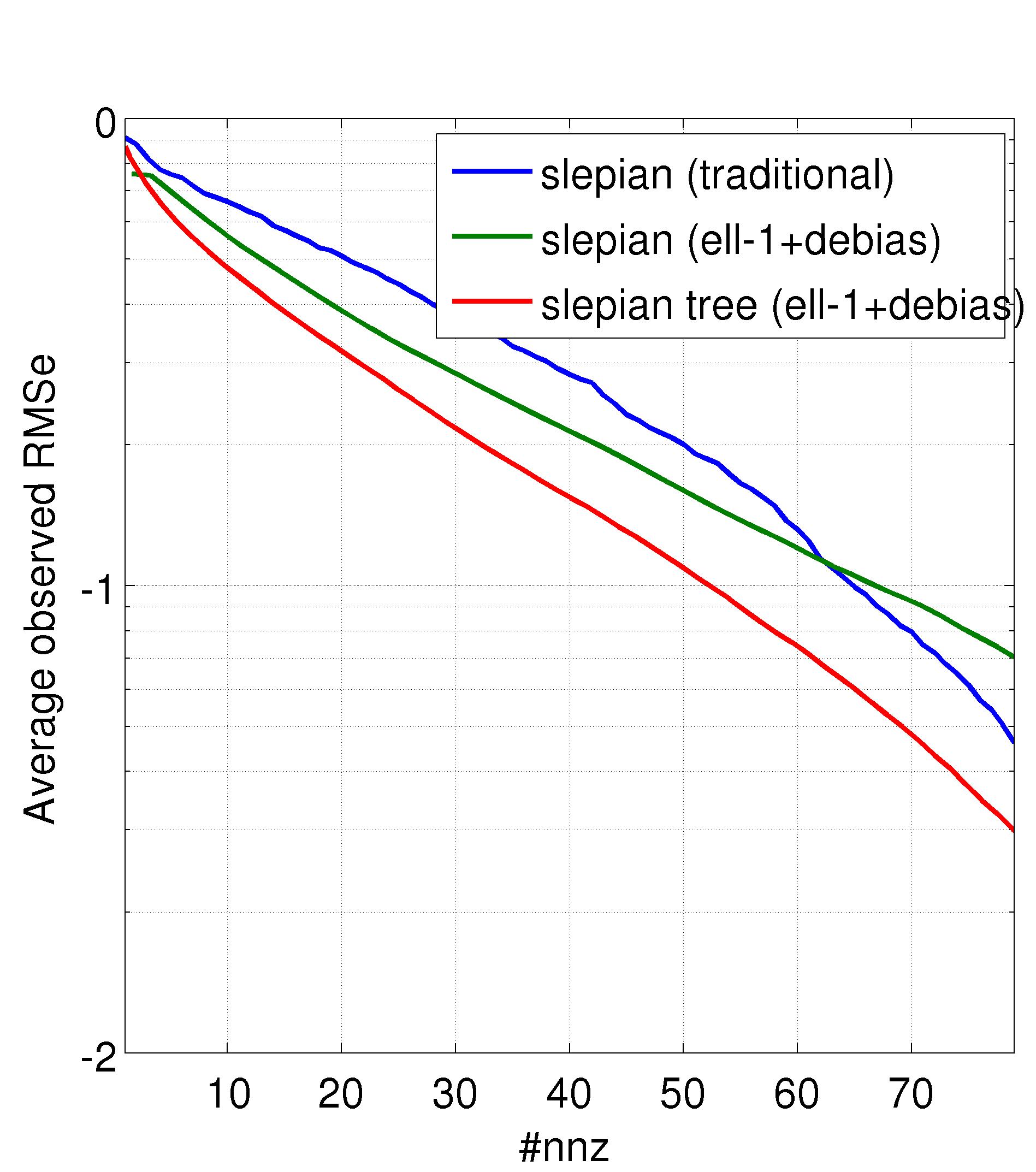
Figure 7.21: Pink noise ($\beta=-2$) average reconstruction error, normalized by signal power within each iteration, on a base-10 log scale. Average taken over $T=200$ iterations. X-axis represents the number of nonzero elements allowed in the support. The Tree dictionary is ${\mathcal{D}}_{\text{Africa},36,1}$.

7.7 Conclusion and Future Work

We have motivated and described a construction for dictionaries of multiscale, bandlimited functions on the sphere. When paired with the modern inversion techniques of §7.5.2, these dictionaries provide a powerful tool for the approximation (inversion) of bandlimited signals concentrated on subsets of the sphere. The numerical examples in §7.6.1 provide good evidence for the efficacy of the estimators SL1D and STL1D. More simulations are required to confirm and explore their numerical accuracy.

In addition, more theoretical analysis of the existing dictionary constructions (e.g., their concentration properties) is also required. Especially when working in concert with the $\ell_{1}$-based estimators, questions of coherence are especially important [44, 17].

The theoretical underpinnings of the SL1D estimator have not been studied, to our knowledge. In contrast, the identically equivalent question of estimating the support of the Fourier transform of a signal, given its (possibly nonuniform) samples, is one that has been studied extensively in the Compressive Sensing community (starting with, e.g., [17, 16]).

The top-down subdivision based scheme described in this chapter is not the only way to construct multiscale dictionaries. Followup work may include one or more of the following ideas:

• Instead of estimating an optimal height $H$ during construction, simply prune a tree element $d^{(j,\alpha)}$ if its spectral concentration $\lambda^{(j,\alpha)}$ or concentration in ${\mathcal{R}}$, $\nu^{(j,\alpha)}$, is below a minimum threshold. This allows for more adaptive and better concentrated dictionary elements near high-curvature borders.

• While the dictionaries described here describe “summary” functions (for $\alpha=1$), it is possible to use Gram-Schmidt orthogonalization to construct an alternate “difference” dictionary by orthogonalizing each node with its parent and sibling. Such dictionaries would be better tuned to find “edges”, and would provide sparser representations for mostly smooth data. In practice, this leads to better performance of $\ell_{1}$-based estimators like STL1D.

• Other subdivision construction schemes should be considered. For example, when the subregion ${\mathcal{R}}$ is highly nonconvex (e.g., when ${\mathcal{R}}$ is the interior of the Earth’s oceans), even the second Slepian function contains more than one mode. In this case, it is unclear how to subdivide the domain from the top down. Instead, a bottom-up approach would work, wherein a fine grid is constructed on the region ${\mathcal{R}}$, and grid elements are “merged” until their area is large enough that reasonably well concentrated Slepian functions with bandwidth $L$ will fit in them.

The ultimate goal of the constructions in this chapter is an overcomplete multiscale frame of bandlimited functions that are well concentrated on ${\mathcal{R}}$, can be constructed quickly, and admit fast forward and inverse transforms. That is, we seek a methodology similar to the Wavelet transforms but allowing for bandlimits. The work here should be considered a stepping stone in that direction as it shares many of the properties of third generation Wavelets treated elsewhere, especially the one that may be most important: numerical accuracy in the solution of ill-posed inverse problems.

Appendix A Differential Geometry: Definitions

The manifold $({\mathcal{M}},g)$ with metric tensor $g$ admits an atlas of charts $\left\{(\phi_{\alpha},U_{\alpha})\right\}_{\alpha}$, where $\phi_{\alpha}:U_{\alpha}\to{\mathbb{R}}^{d}$ is a diffeomorphism from the open subset $U_{\alpha}\subset{\mathcal{M}}$ [33, Chs. 0,4]. The choice of a standard orthonormal basis in ${\mathbb{R}}^{d}$ defines a corresponding basis for the tangent plane to ${\mathcal{M}}$ at each $x\in U_{\alpha}$, as well as a local coordinate system $\left\{v^{j}\right\}$ near $x$. The components of the tensor $g$ are defined as the inner products between the partial derivatives of $\phi_{\alpha}$ in this coordinate system: $g_{ij}(x)=\left\langle{\partial\phi_{\alpha}(x)/\partial v^{i}},{\partial\phi_{\alpha}(x)/\partial v^{j}}\right\rangle$ where $v=\phi_{\alpha}(x)$. The inverse tensor, denoted by $g^{ik}(x)=(g^{-1}(x))_{ik}$, is smooth, everywhere symmetric and positive definite because $g$ is. We use the notation $\left\lvert g\right\rvert=\det{(g_{ij})}$. Note that we will often drop the position term $x$; for example, $g^{-1}=g^{-1}(x)$.

We assign to ${\mathcal{M}}$ the standard gradient $\nabla$, inner product $\cdot$, divergence $\nabla\cdot$, and Laplacian $\Delta=\nabla\cdot\nabla$ at a point $x$ [83, Ch. 1]. For $f$ a twice-differentiable function on ${\mathcal{M}}$ (i.e. $f\in C^{2}({\mathcal{M}})$) and $\bm{f}$ and $\bm{g}$ differentiable vector fields on ${\mathcal{M}}$,

$$\partial_{i}f(x)=\frac{\partial f(x)}{\partial v^{i}}\qquad(\nabla f)^{j}=\sum_{i}g^{ij}(x)\partial_{i}f(x)\qquad\bm{f}\cdot\bm{g}=\sum_{i,j}g_{ij}(x)\bm{f}^{i}(x)\bm{f}^{j}(x)$$

$$\nabla\cdot\bm{f}=\sum_{i}\frac{1}{\sqrt{\left\lvert g(x)\right\rvert}}\partial_{i}\left(\sqrt{\left\lvert g(x)\right\rvert}\bm{f}^{i}(x)\right)\qquad\Delta f=\sum_{i,j}\frac{1}{\sqrt{\left\lvert g(x)\right\rvert}}\partial_{i}\left(\sqrt{\left\lvert g(x)\right\rvert}g^{ij}(x)\partial_{j}f(x)\right),$$

where again $v=\phi_{\alpha}(x)$ and $1\leq i,j,k\leq d$. We use the definitions above throughout, as well as the norm definition $\left\lVert\bm{f}\right\rVert^{2}=\bm{f}\cdot\bm{f}$; thus $\left\lVert\nabla f\right\rVert^{2}=\sum_{i,j}g^{ij}\partial_{i}f\partial_{j}f$.

Appendix B Spectral Theory

In this appendix we state some basic facts about the existence of the Fourier transform for functions in $L^{2}({\mathbb{R}}^{n})$. We also discuss the existence and properties of Fourier series representations for functions in $L^{2}({\mathcal{M}})$, where $({\mathcal{M}},g)$ is a Riemannian manifold with metric $g$ (see App. A). A comprehensive review of Fourier transforms and convolutions on general (possibly non-compact) spaces is available in [86, Ch. 7], and on Riemannian Manifolds in particular in [83, Ch. 1].

B.1 Fourier Transform on ${\mathbb{R}}^{n}$

The Fourier transform of a function $f\in L^{2}({\mathbb{R}}^{n})$ is formally defined, for all $\omega\in{\mathbb{R}}^{n}$, as

$$\widehat{f}(\omega)=\int_{x\in{\mathbb{R}}^{n}}f(x)\overline{\psi_{\omega}(x)}dx,$$

where $\psi_{\omega}(x)=e^{ix\cdot\omega}$ solves the eigenvalue problem

$$\Delta\psi_{\omega}(x)=-\lambda_{\omega}^{2}\psi_{\omega}(x),\qquad x\in{\mathbb{R}}^{n}$$

with $\Delta f(x)=\sum_{j=1}^{n}\frac{\partial^{2}}{\partial x_{j}^{2}}f(x)$ and $\lambda_{\omega}=\left\lVert\omega\right\rVert_{2}$.

The Fourier inversion theorem and its extensions [86, Thms. 7.7 and 7.15] state that $\widehat{f}$ is well defined, and that $f$ can be represented via $\widehat{f}$. For all $x\in{\mathbb{R}}^{n}$,

$$f(x)=(2\pi)^{-n}\int_{\omega\in{\mathbb{R}}^{n}}\widehat{f}(\omega)\psi_{\omega}(x)dx.$$

B.2 Fourier Analysis on Riemannian Manifolds

Suppose ${\mathcal{H}}$ is a separable Hilbert space, e.g., ${\mathcal{H}}=L^{2}(M)$ where $M$ is a compact set. Further, suppose $T:{\mathcal{H}}\to{\mathcal{H}}$ is a bounded, compact, self-adjoint operator. Then the Hilbert-Schmidt theorem [81, Thm. VI.16] states that there is a complete orthonormal basis $\left\{\psi_{k}\right\}$ for ${\mathcal{H}}$ such that $T\psi_{k}(x)=\lambda_{k}\psi_{k}(x)$, $k=0,1,\ldots$, and $\lambda_{k}\to 0$ as $k\to\infty$. The Laplacian operator $T=\Delta$ defined on compact subsets of $M\subset{\mathbb{R}}^{n}$ therefore admits a complete orthonormal basis (as its inverse is compact), and from now on we refer to $\left\{\psi_{k}\right\}$ as the eigenfunctions of the Laplacian. This set is called the Fourier basis.

We can therefore write any function $f\in L^{2}(M)$ as

$$f(x)=\sum_{k=0}^{\infty}\widehat{f}_{k}\psi_{k}(x)\qquad\text{where}\qquad\widehat{f}_{k}=\int_{M}f(x)\overline{\psi_{k}(x)}dx,$$

where $\left\{\widehat{f}_{k}\right\}$ are called the Fourier coefficients. The calculation of Fourier coefficients is called analysis, and the reconstruction of $f$ by expansion in the Fourier basis is called synthesis.

On a Riemannian manifold $({\mathcal{M}},g)$ a similar analysis applies [83, Thm. 1.29]:

Proposition B.2.1 (Hodge Theorem for Functions).

Let $({\mathcal{M}},g)$ be a compact connected oriented Riemannian manifold. There exists an orthonormal basis of $L^{2}({\mathcal{M}})$ consisting of eigenfunctions of the Laplacian. All the eigenvalues are positive, except that zero is an eigenvalue with multiplicity one. Each eigenvalue has finite multiplicity, and the eigenvalues accumulate only at infinity.

The Laplacian given above is the negative of the Laplace-Beltrami operator defined in §A, and the eigenfunctions have Neumann boundary conditions.

Fourier analysis and synthesis can be written as

$$f(x)=\sum_{k=0}^{\infty}\widehat{f}_{k}\psi_{k}(x),x\in{\mathcal{M}}\qquad\text{where}\qquad\widehat{f}_{k}=\int_{\mathcal{M}}f(x)\overline{\psi_{k}(x)}d\mu(x),$$

where the analysis integral above is with respect to the volume metric $g$. Fourier analysis is a unitary operation (this is known as Parseval’s theorem). Note that practical definitions of the forward and inverse Fourier operators often differ by the choice and placement of normalization constants, in order to simplify notation (as is the case throughout this thesis).

B.2.1 Fourier Analysis on the Circle $S^{1}$

On the circle, $S^{1}$, parametrized by $\left\{\theta:\theta\in[0,2\pi)\right\}$ with $d\mu(\theta)=d\theta$, we have $\Delta e^{i\theta k}=-k^{2}e^{ik\theta}$ for $k=0,\pm 1,\pm 2,\ldots$. We can therefore decompose $L^{2}(S^{1})$ via projections onto $\left\{e^{i\theta k}\right\}_{k}$. That is, we can write

$$f(\theta)=\sum_{k=-\infty}^{\infty}\widehat{f}_{k}e^{i\theta k}\qquad\text{where}\qquad\widehat{f}_{k}=\frac{1}{2\pi}\int_{S^{1}}f(\theta)e^{-i\theta k}d\theta$$

for any $f\in L^{2}(S^{1})$.

The analysis, as defined, is an isometry. By Parseval’s theorem, for $f,g\in L^{2}(S^{1})$,

$$\int_{S^{1}}f(\theta)\overline{g(\theta)}d\theta=\sum_{k=-\infty}^{\infty}\widehat{f}_{k}\overline{\widehat{g}_{k}}$$

This analysis can also be applied to functions on $L^{2}[0,2\pi]$ with periodic boundary conditions by identifying the interval with $S^{1}$.

B.2.2 Fourier Analysis on the Sphere $S^{2}$

The unit sphere, $S^{2}$, can be parametrized by $\left\{(\theta,\phi):\theta\in[0,\pi],\phi\in[0,2\pi)\right\}$ where $\theta$ is the colatitude and $\phi$ is the longitude. In this case, the Laplacian is

$$\Delta f(\theta,\phi)=\frac{1}{\sin\theta}\partial_{\theta}\left(\sin\theta\partial_{\theta}f(\theta,\phi)\right)+\frac{1}{\sin^{2}\theta}\partial_{\phi\phi}f(\theta,\phi)$$

and the volume element is $d\mu(\theta,\phi)=\sin\theta d\phi d\theta$.

For our purposes, we are interested in real-valued functions on the sphere. As such, we study the real-valued eigenfunctions of the Laplacian on $S^{2}$. The real surface spherical harmonics, $\left\{Y_{lm}(\theta,\phi)\right\}$, are parametrized by the degree $l$ and order $m$, where $l=0,1,\ldots$ and $m=-l,\ldots,l$. These can be given by [91]:

$$Y_{lm}(\theta,\phi) =\begin{cases}\sqrt{2}X_{l\left\lvert m\right\rvert}(\theta)\cos(m\theta)&-l\leq m<0,\\ X_{l0}(\theta)&m=0,\\ \sqrt{2}X_{lm}(\theta)\sin(m\theta)&0<m\leq l,\end{cases}\qquad\text{where}$$ (B.1)

$$X_{lm}(\theta) =(-1)^{m}\left(\frac{(2l+1)}{4\pi}\frac{(l-m)!}{(l+m)!}\right)^{1/2}P_{lm}(\cos\theta),$$ (B.2)

and $P_{lm}(t)$ are the associated Legendre functions of degree $l$ and degree $m$ [1, §8.1.1]. Each spherical harmonic $Y_{lm}$ fulfills the eigenvalue relationship $\Delta Y_{lm}=-l(l+1)Y_{lm}$.

We can therefore decompose $L^{2}(S^{2},{\mathbb{R}})$ via projections onto $\left\{Y_{lm}(\theta,\phi)\right\}_{lm}$, where now $\overline{Y_{lm}}=Y_{lm}$. That is, we can write

$$f(\theta,\phi)=\sum_{lm}\widehat{f}_{lm}Y_{lm}(\theta,\phi)\qquad\text{where}\qquad\widehat{f}_{lm}=\int_{S^{2}}f(\theta,\phi)Y^{m}_{l}(\theta,\phi)d\mu(\theta,\phi),$$

for any $f\in L^{2}(S^{2},{\mathbb{R}})$.

The analysis, as defined, is an isometry. By a Parseval’s theorem, for real-valued functions $f,g\in L^{2}(S^{2})$,

$$\int_{S^{2}}f(\theta,\phi)g(\theta,\phi)d\mu(\theta,\phi)=\sum_{l\geq 0}\sum_{m=-l}^{l}\widehat{f}_{lm}\widehat{g}_{lm}.$$

References

- [1] M. Abramowitz and I. Stegun, Handbook of mathematical functions with formulas, graphs, and mathematical tables, Dover publications, 1964.
- [2] D. Azagra, J. Ferrera, and B. Sanz, Viscosity solutions to second order partial differential equations on Riemannian manifolds, Journal of Differential Equations, 245 (2008), pp. 307–336.
- [3] M. Balasubramanian and E. L. Schwartz, The isomap algorithm and topological stability, Science, 295 (2002), p. 7.
- [4] M. Belkin, I. Matveeva, and P. Niyogi, Regularization and semi-supervised learning on large graphs, Learning theory, (2004), pp. 624–638.
- [5] M. Belkin and P. Niyogi, Towards a theoretical foundation for Laplacian-based manifold methods, Journal of Computer and System Sciences, 74 (2008), pp. 1289–1308.
- [6] M. Belkin, P. Niyogi, and V. Sindhwani, Manifold regularization: a geometric framework for learning from labeled and unlabeled examples, JMLR, 7 (2006), pp. 2399–2434.
- [7] M. Belkin, J. Sun, and Y. Wang, Discrete Laplace operator on meshed surfaces, in Proceedings of the twenty-fourth annual symposium on Computational geometry, ACM, 2008, pp. 278–287.
- [8] Y. Bengio, J. Paiement, P. Vincent, O. Delalleau, N. Le Roux, and M. Ouimet, Out-of-sample extensions for lle, isomap, mds, eigenmaps, and spectral clustering, in Advances in Neural Information Processing Systems 16: Proceedings of the 2003 Conference, The MIT Press, 2004, p. 177.
- [9] A. Berger and M. Loutre, Astronomical solutions for paleoclimate studies over the last 3 million years, Earth and Planetary Science Letters, 111 (1992), pp. 369–382.
- [10] C. Bishop, Pattern recognition and machine learning, vol. 4, Springer New York, 2006.
- [11] U. Brandes, A faster algorithm for betweenness centrality, Journal of Mathematical Sociology, 25 (2001), p. 163–177.
- [12] E. Brevdo, N. Fučkar, G. Thakur, and H. Wu, The Synchrosqueezing algorithm: a robust analysis tool for signals with time-varying spectrum., Submitted (Arxiv preprint arXiv:1105.0010), (2011).
- [13] E. Brevdo and P. Ramadge, Bridge detection and robust geodesics estimation via random walks, IEEE Int. Conference on Acoustics, Speech & Signal Processing, March 2010.
- [14] , Semisupervised learning: the regularized Laplacian, geodesics, and the small viscosity limit, Submitted, (2011).
- [15] E. Candès and J. Romberg, Sparsity and incoherence in compressive sampling, Inverse problems, 23 (2007), p. 969.
- [16] E. Candès, J. Romberg, and T. Tao, Robust uncertainty principles: Exact signal reconstruction from highly incomplete frequency information, Information Theory, IEEE Transactions on, 52 (2006), pp. 489–509.
- [17] E. Candes, J. Romberg, and T. Tao, Stable signal recovery from incomplete and inaccurate measurements, Communications on pure and applied mathematics, 59 (2006), pp. 1207–1223.
- [18] H. Chang and D. Yeung, Robust locally linear embedding, Pattern Recognition, 39 (2006), pp. 1053–1065.
- [19] O. Chapelle, B. Schölkopf, and A. Zien, eds., Semi-Supervised Learning, MIT Press, Cambridge, MA, 2006.
- [20] O. Chapelle and A. Zien, Semi-supervised classification by low density separation, in Proceedings of the tenth international workshop on artificial intelligence and statistics, vol. 2005, 2005.
- [21] H. Chen, G. Jiang, and K. Yoshihira, Robust nonlinear dimensionality reduction for manifold learning, ICPR, 1 (2006), pp. 447–450.
- [22] P. Clark, D. Archer, D. Pollard, J. Blum, J. Rial, V. Brovkin, A. Mix, N. Pisias, and M. Roy, The middle Pleistocene transition: characteristics, mechanisms, and implications for long-term changes in atmospheric pCO2, Quaternary Science Reviews, 25 (2006), pp. 3150–3184.
- [23] R. Coifman and S. Lafon, Diffusion maps, Applied and Computational Harmonic Analysis, 21 (2006), pp. 5–30.
- [24] R. R. Coifman, S. Lafon, A. B. Lee, M. Maggioni, B. Nadler, F. Warner, and S. W. Zucker, Geometric diffusions as a tool for harmonic analysis and structure definition of data: diffusion maps, PNAS, 102 (2005), pp. 7426–31.
- [25] T. Cormen, C. Leiserson, R. Rivest, and C. Stein, Introduction to algorithms., Cambridge, MA: MIT Press, 2001.
- [26] M. G. Crandall, H. Ishii, and P.-L. Lions, User’s guide to viscosity solutions of second order partial differential equations, Bulletin of the American Mathematical Society, 27 (1992), pp. 1–68.
- [27] F. A. Dahlen and F. J. Simons, Spectral estimation on a sphere in geophysics and cosmology, Geophysical Journal International, 174 (2008), pp. 774–807.
- [28] A. d’Aspremont and L. El Ghaoui, Testing the nullspace property using semidefinite programming, Mathematical Programming, (2008), pp. 1–22.
- [29] I. Daubechies, Ten lectures on wavelets, Society for Industrial Mathematics, 1992.
- [30] I. Daubechies, R. DeVore, M. Fornasier, and C. Güntürk, Iteratively reweighted least squares minimization for sparse recovery, Communications on Pure and Applied Mathematics, 63 (2010), pp. 1–38.
- [31] I. Daubechies, J. Lu, and H.-T. Wu, Synchrosqueezed wavelet transforms: An empirical mode decomposition-like tool, Applied and Computational Harmonic Analysis, (2010).
- [32] I. Daubechies and S. Maes, A nonlinear squeezing of the continuous wavelet transform based on auditory nerve models, Wavelets in Medicine and Biology, (1996), pp. 527–546.
- [33] M. P. do Carmo, Riemannian Geometry, Birkhäuser, Boston, MA, 1992.
- [34] D. Donoho, Compressed sensing, Information Theory, IEEE Transactions on, 52 (2006), pp. 1289–1306.
- [35] J. Driscoll and D. Healy, Computing fourier transforms and convolutions on the 2-sphere, Advances in Applied Mathematics, 15 (1994), pp. 202–250.
- [36] W. Einthoven, G. Fahr, and A. Waart, On the Direction and Manifest Size of the Variations of Potential in the Human Heart and on the Influence of the Position of the Heart on the Form of the Electrocardiogram, Am. Heart J., 40 (1950).
- [37] M. Eshagh, Spatially restricted integrals in gradiometric boundary value problems, Artificial Satellites, 44 (2009), pp. 131–148.
- [38] L. C. Evans, Partial Differential Equations (Graduate Studies in Mathematics, V. 19) GSM/19, American Mathematical Society, June 1998.
- [39] J. Flaherty, S. Blumenschein, A. Alexander, R. Gentzler, T. Gallie, J. Boineau, and M. Spach, Influence of respiration on recording cardiac potentials:: Isopotential surface-mapping and vectorcardiographic studies, The American Journal of Cardiology, 20 (1967), pp. 21–28.
- [40] P. Flandrin, Time-frequency/time-scale analysis, vol. 10 of Wavelet Analysis and its Applications, Academic Press Inc., San Diego, CA, 1999.
- [41] P. Flandrin, F. Auger, and E. Chassande-Mottin, Time-frequency reassignment – from principles to algorithms, in Applications in time-frequency signal processing, A. Papandreou-Suppappola, ed., CRC, 2003.
- [42] S. Fulop and K. Fitz, Algorithms for computing the time-corrected instantaneous frequency (reassigned) spectrogram, with applications, J. Acoust. Soc. Am., 119 (2006), p. 360.
- [43] P. Goupillaud, A. Grossmann, and J. Morlet, Cycle-octave and related transforms in seismic signal analysis, Geoexploration, 23 (1984), pp. 85–102.
- [44] S. Gurevich and R. Hadani, Incoherent dictionaries and the statistical restricted isometry property, Arxiv preprint arXiv:0809.1687, (2008).
- [45] J. Ham, D. D. Lee, S. Mika, and B. Schölkopf, A kernel view of the dimensionality reduction of manifolds, in ICML, ACM New York, NY, USA, 2004.
- [46] J. Hays, J. Imbrie, N. Shackleton, et al., Variations in the Earth’s orbit: pacemaker of the ice ages, Science, 194 (1976), pp. 1121–1132.
- [47] M. Hazewinkel and I. Vinogradov, Encyclopaedia of mathematics, Kluwer Academic Publishers, 1995.
- [48] M. Hein, J. Audibert, and U. Von Luxburg, From graphs to manifolds–weak and strong pointwise consistency of graph Laplacians, Learning theory, (2005), pp. 470–485.
- [49] R. Horn and C. Johnson, Matrix analysis, Cambridge University Press New York, NY, USA, 1985.
- [50] N. Huang, Z. Shen, S. Long, M. Wu, H. Shih, Q. Zheng, N. Yen, C. Tung, and H. Liu, The empirical mode decomposition and the Hilbert spectrum for nonlinear and non-stationary time series analysis, Proceedings: Mathematical, Physical and Engineering Sciences, 454 (1998), pp. 903–995.
- [51] P. Huybers, Glacial variability over the last two million years: an extended depth-derived agemodel, continuous obliquity pacing, and the Pleistocene progression, Quaternary Science Reviews, 26 (2007), pp. 37–55.
- [52] P. Huybers and W. Curry, Links between annual, Milankovitch and continuum temperature variability, Nature, 441 (2006), pp. 329–332.
- [53] P. W. Jones, M. Maggioni, and R. Schul, Manifold parametrizations by eigenfunctions of the laplacian and heat kernels, PNAS, 105 (2008), p. 1803.
- [54] J. Jost, Riemannian Geometry and Geometric Analysis, Springer, 3rd ed., 2001.
- [55] A. Juditsky and A. Nemirovski, On verifiable sufficient conditions for sparse signal recovery via minimization, Mathematical Programming, (2008), pp. 1–32.
- [56] K. Kim, F. Steinke, and M. Hein, Semi-supervised regression using Hessian energy with an application to semi-supervised dimensionality reduction, 22 (2009).
- [57] R. Kimmel and J. Sethian, Computing geodesic paths on manifolds, Proceedings of the National Academy of Sciences of the United States of America, 95 (1998), p. 8431.
- [58] S. N. Kruzkov, Generalized solutions of the hamilton-jacobi equations of eikonal type. i. formulation of the problems; existence, uniqueness and stability theorems; some properties of the solutions, Mathematics of the USSR-Sbornik, 27 (1975), pp. 406–446.
- [59] C. Kubrusly, Measure theory: a first course, Academic Press, 2007.
- [60] S. Lafon, Diffusion maps and geometric harmonics, PhD thesis, Yale University, 2004.
- [61] H. Landau and H. Pollak, Prolate spheroidal wave functions, fourier analysis and uncertainty ii., Bell Syst. Tech. J, 40 (1961), pp. 65–84.
- [62] , Prolate spheroidal wave functions, fourier analysis and uncertainty. iii. the dimension of the space of essentially time-and band-limited signals, Bell Syst. Tech. J, 41 (1962), pp. 1295–1336.
- [63] B. Li, D.-S. Huang, and C. Wang, Improving the robustness of isomap by de-noising, IJCNN, (2008), pp. 266–270.
- [64] P. Lions, Generalized solutions of Hamilton–Jacobi equations, Pitman Boston-London, 1982.
- [65] U. Luxburg, A tutorial on spectral clustering, Statistics and Computing, 17 (2007), p. 416.
- [66] M. Malik and J. Camm, Dynamic Electrocardiography, Wiley, 2004.
- [67] S. Mallat, A Wavelet Tour of Signal Processing, Third Edition: The Sparse Way, Academic Press, 3 ed., Dec. 2008.
- [68] C. Mantegazza and A. C. Mennucci, Hamilton–Jacobi equations and distance functions on Riemannian manifolds, Applied Mathematics and Optimization, 47 (2002), pp. 1–25.
- [69] S. Maus, U. Barckhausen, H. Berkenbosch, N. Bournas, J. Brozena, V. Childers, F. Dostaler, J. Fairhead, C. Finn, R. von Frese, et al., Emag2: A 2–arc min resolution earth magnetic anomaly grid compiled from satellite, airborne, and marine magnetic measurements, Geochemistry Geophysics Geosystems, 10 (2009), p. Q08005.
- [70] S. Maus, M. Rother, C. Stolle, W. Mai, S. Choi, H. Lühr, D. Cooke, and C. Roth, Third generation of the potsdam magnetic model of the earth (pomme), Geochem. Geophys. Geosyst, 7 (2006).
- [71] F. Memoli and G. Sapiro, Distance functions and geodesics on submanifolds of and point clouds, SIAM Journal on Applied Mathematics, 65 (2005), p. 1227.
- [72] M. B. Monagan, K. O. Geddes, K. M. Heal, G. Labahn, S. M. Vorkoetter, J. McCarron, and P. DeMarco, Maple 10 Programming Guide, Maplesoft, Waterloo ON, Canada, 2005.
- [73] G. B. Moody, R. G. Mark, A. Zoccola, and M. S., Derivation of respiratory signals from multi-lead ECGs, Computers in Cardiology, (1985).
- [74] B. Nadler, N. Srebro, and X. Zhou, Semi-supervised learning with the graph Laplacian: the limit of infinite unlabelled data, in Advances in Neural Information Processing Systems, vol. 22, 2009.
- [75] A. Nayfeh, Perturbation methods, vol. 6, Wiley Online Library, 1973.
- [76] M. Newman and M. Girvan, Finding and evaluating community structure in networks, Phys. Rev. E, 69 (2004), pp. 1–15.
- [77] A. Oppenheim, R. Schafer, and J. Buck, Discrete-Time Signal Processing, Prentice Hall, 1999.
- [78] M. Paul, Recurrence relations for integrals of associated legendre functions, Journal of Geodesy, 52 (1978), pp. 177–190.
- [79] R. Pierrehumbert, Principles of planetary climate, Cambridge University Press, 2010.
- [80] M. Raymo and P. Huybers, Unlocking the mysteries of the ice ages, Nature, 451 (2008), pp. 284–285.
- [81] M. Reed and B. Simon, Methods of modern mathematical physics, Academic press, 1980.
- [82] F. Riesz and B. Nagy, Functional analysis. (Translated from the 2nd French edition by LF Boron)., 1956.
- [83] S. Rosenberg, The Laplacian on a Riemannian manifold: an introduction to analysis on manifolds, Cambridge Univ Press, 1997.
- [84] W. Ruddiman, M. Raymo, D. Martinson, B. Clement, and J. Backman, Pleistocene evolution: northern hemisphere ice sheets and North Atlantic Ocean, Paleoceanography, 4 (1989), pp. 353–412.
- [85] W. Ruddiman, M. Raymo, and A. McIntyre, Matuyama 41,000-year cycles: North Atlantic Ocean and northern hemisphere ice sheets, Earth and Planetary Science Letters, 80 (1986), pp. 117–129.
- [86] W. Rudin, Functional Analysis, McGraw-Hill, New York, 1973.
- [87] Z. Schuss and A. Spivak, On recovering the shape of a domain from the trace of the heat kernel, Arxiv preprint math-ph/0501008, (2005).
- [88] J. Sethian and A. Vladimirsky, Fast methods for the Eikonal and related Hamilton–Jacobi equations on unstructured meshes, Proceedings of the National Academy of Sciences of the United States of America, 97 (2000), p. 5699.
- [89] C. Shannon, Communication in the presence of noise, Proceedings of the IRE, 37 (1949), pp. 10–21.
- [90] F. J. Simons, Slepian functions and their use in signal estimation and spectral analysis, in The Handbook of Geomathematics, W. Freeden, Z. M. Nashed, and T. Sonar, eds., Springer Verlag, 2010.
- [91] F. J. Simons and F. A. Dahlen, Spherical Slepian functions and the polar gap in geodesy, Geophysical Journal International, 166 (2006), pp. 1039–1061.
- [92] F. J. Simons and F. A. Dahlen, A spatiospectral localization approach to estimating potential fields on the surface of a sphere from noisy, incomplete data taken at satellite altitudes, in Proc. of SPIE Vol, vol. 6701, 2007.
- [93] F. J. Simons, F. A. Dahlen, and M. A. Wieczorek, Spatiospectral concentration on a sphere, SIAM Review, 48 (2006), p. 504.
- [94] A. Singer, From graph to manifold laplacian: The convergence rate, Applied and Computational Harmonic Analysis, 21 (2006), pp. 128 – 134.
- [95] A. Singer, R. Coifman, F. Sigworth, D. Chester, and Y. Shkolnisky, Detecting consistent common lines in cryo-em by voting, Journal of structural biology, 169 (2010), pp. 312–322.
- [96] A. Singer and H. Wu, 2-d tomography from noisy projections taken at unknown random directions, Submitted, (2009).
- [97] A. Singer and H. Wu, Vector diffusion maps and the connection laplacian, Arxiv preprint arXiv:1102.0075, (2011).
- [98] D. Slepian, Prolate spheroidal wave functions, fourier analysis, and uncertainty. v-the discrete case, Bell Syst. Tech. J, 57 (1978), pp. 1371–1430.
- [99] D. Slepian and H. O. Pollak, Prolate spheroidal wave functions, fourier analysis, and uncertainty-i, Bell System Tech. J., 40 (1961), pp. 43–64.
- [100] D. C. Slobbe, F. J. Simons, and R. Klees, The spherical slepian basis as a means to obtain spectral consistency between mean sea level and the geoid, Journal of Geodesy, (2011).
- [101] A. Smola and R. Kondor, Kernels and regularization on graphs, in Learning theory and Kernel machines: 16th Annual Conference on Learning Theory and 7th Kernel Workshop, COLT/Kernel 2003, Washington, DC, USA, August 24-27, 2003: proceedings, Springer Verlag, 2003, p. 144.
- [102] G. Stewart, Afternotes goes to graduate school: lectures on advanced numerical analysis, Society for Industrial Mathematics, 1998.
- [103] R. Subbarao and P. Meer, Subspace estimation using projection based m-estimators over grassmann manifolds, ECCV, 3951 (2006), pp. 301–312.
- [104] E. Tadmor, The exponential accuracy of Fourier and Chebyshev differencing methods, SIAM Journal on Numerical Analysis, 23 (1986), pp. 1–10.
- [105] J. Tenenbaum, V. Silva, and J. Langford, A global geometric framework for nonlinear dimensionality reduction, Science, 290 (2000), p. 2319.
- [106] G. Thakur and H. Wu, Synchrosqueezing-based recovery of instantaneous frequency from nonuniform samples, Submitted (Arxiv preprint arXiv:1006.2533), (2010).
- [107] R. Tibshirani, Regression shrinkage and selection via the lasso, Journal of the Royal Statistical Society. Series B (Methodological), 58 (1996), pp. 267–288.
- [108] D. Ting, L. Huang, and M. Jordan, An analysis of the convergence of graph laplacians, Tech. Rep. 792, Statistics Department – University of California Berkeley, July 2010.
- [109] D. Trudinger and N. S. Gilbarg, Elliptic partial differential equations of second order, Springer-Verlag, Berlin, second ed., 1983.
- [110] J. M. Wahr, M. Molenaar, and F. Bryan, Time variability of the Earth’s gravity field: Hydrological and oceanic effects and their possible detection using GRACE, JGR, 103 (1998), pp. 30205–30229.
- [111] P. Wedin, On angles between subspaces of a finite dimensional inner product space, Matrix Pencils, (1983), pp. 263–285.
- [112] M. A. Wieczorek and F. J. Simons, Localized spectral analysis on the sphere, Geophysical Journal International, 162 (2005), pp. 655–675.
- [113] P. Xu, Truncated svd methods for discrete linear ill-posed problems, Geophysical Journal International, 135 (1998), pp. 505–514.
- [114] D. Zhou and B. Schölkopf, Learning from labeled and unlabeled data using random walks, in Pattern Recognition: 26th DAGM Symp., Springer, 2004, pp. 237–244.
- [115] X. Zhu, Z. Ghahramani, and J. Lafferty, Semi-supervised learning using Gaussian fields and harmonic functions, in International Conference on Machine Learning, vol. 20, 2003, p. 912.