A projection-based model reduction method for nonlinear mechanics with internal variables: application to thermo-hydro-mechanical systems.

Abstract

We propose a projection-based monolithic model order reduction (MOR) procedure for a class of problems in nonlinear mechanics with internal variables. The work is is motivated by applications to thermo-hydro-mechanical (THM) systems for radioactive waste disposal. THM equations model the behaviour of temperature, pore water pressure and solid displacement in the neighborhood of geological repositories, which contain radioactive waste and are responsible for a significant thermal flux towards the Earth’s surface. We develop an adaptive sampling strategy based on the POD-Greedy method, and we develop an element-wise empirical quadrature hyper-reduction procedure to reduce assembling costs. We present numerical results for a two-dimensional THM system to illustrate and validate the proposed methodology.

Angelo Iollo¹, Giulia Sambataro¹, Tommaso Taddei¹,

¹ IMB, UMR 5251, Univ. Bordeaux; 33400, Talence, France. Inria Bordeaux Sud-Ouest, Team MEMPHIS; 33400, Talence, France, angelo.iollo@inria.fr,giulia.sambataro@inria.fr,tommaso.taddei@inria.fr

Keywords: parameterized partial differential equations; model order reduction; nonlinear mechanics.

1 Introduction

1.1 Model reduction for a class of models in nonlinear mechanics

The disposal and storage of high-level radioactive waste materials in geological means requires a careful assessment of the long-term effects on neighboring areas. The system behaviour is well-described by time-dependent large-scales coupled systems of partial differential equations (PDEs), which take into account the thermal, hydraulic and mechanical response of the geological medium. Numerical simulation of these systems is challenging due to several difficulties: first, finite element (FE) models of the problem are highly-nonlinear, time-dependent and high-dimensional; second, due to the uncertainty in model parameters, we need to solve the model for many different system configurations (many-query problem). In this work, we shall devise a model-order reduction (MOR) strategy to speed up parametric studies for radio-active waste disposal applications.

In this contribution we study a general class of nonlinear problems in structural mechanics with internal variables. We consider the spatial variable $x$ in the Lipschitz domain $\Omega\subset\mathbb{R}^{d}$ with $d=2,3$, and the time variable $t$ in the time internal $(0,T_{\rm{f}})$, where $T_{\rm{f}}$ is the final time. We further define the vector of parameters $\mu$ in the compact parameter region $\mathcal{P}\subset\mathbb{R}^{P}$. We introduce the state (or primary) variables $\underline{U}$ and internal (or dependent) variables $\underline{W}$; we denote by $\mathcal{X}$ and $\mathcal{W}$ suitable Hilbert spaces in $\Omega$ for $\underline{U}$ and $\underline{W}$, and we define the space of continuous functions from $(0,T_{\rm{f}})$ to $\mathcal{X}$ and $\mathcal{W}$, $C(0,T_{\rm{f}};\mathcal{X})$ and $C(0,T_{\rm{f}};\mathcal{W})$. Then, we introduce the parameterised problem of interest: given $\mu\in\mathcal{P}$, find $(\underline{U}_{\mu},\underline{W}_{\mu})\in C(0,T_{\rm{f}};\mathcal{X})\times C(0,T_{\rm{f}};\mathcal{W})$ such that

$$\left\{\begin{array}[]{ll}\displaystyle{\mathcal{G}_{\mu}(\underline{U}_{\mu},\partial_{\rm{t}}\underline{U}_{\mu},\underline{W}_{\mu})=0}&{\rm in}\,\Omega\times(0,T_{\rm{f}})\\[8.53581pt] \displaystyle{\dot{\underline{W}}_{\mu}=\mathcal{F}_{{\mu}}(\underline{U}_{\mu},\underline{W}_{\mu})},&{\rm in}\,\Omega\times(0,T_{\rm{f}})\\ \end{array}\right.$$ (1)

with suitable initial and boundary conditions. Here, $\mathcal{G}_{\mu}$ is a nonlinear second-order in space, first-order in time differential operator that is associated with the equilibrium equations, while $\mathcal{F}_{{\mu}}$ is a set of ordinary differential equations (ODEs) that is associated with the constitutive laws.

Our methodology is motivated by the application to thermo-hydro-mechanical (THM) systems of the form (1), which are widely used to model the system’s response for radio-active waste disposal applications. Radioactive material is placed in an array of horizontal boreholes (dubbed alveoli) deep underground: due to the large temperature of the alveoli, a thermal flux is generated; the thermal flux then drives the mechanical and hydraulic response of the medium over the course of several years. We refer to section 4 for a detailed discussion of the considered THM model and boundary conditions.

1.2 Objective of the work and relationship to previous works

We propose a projection-based monolithic model order reduction (MOR ) ([15, 23, 25]) technique for problems of the form (1), with particular emphasis on THM systems. The approach is characterised by an offline/online splitting to reduce the marginal cost, and relies on Galerkin projection to devise a reduced-order model (ROM) for the solution coefficients. We rely on hyper-reduction to speed up the assembly of the ROM during the online stage, and we rely on adaptive sampling to reduce the offline training costs.

The contribution of the present work is twofold. First, we propose an element-wise empirical quadrature (EQ) procedure for problems with internal variables; second, we extend the POD-Greedy algorithm and we propose an error indicator that is effective to drive the offline greedy search and is inexpensive to evaluate.

EQ procedures also dubbed mesh sampling and weighting have been first proposed in [9, 32, 33] and further developed in several other works including [24]: the key feature of EQ is to recast the problem of hyper-reduction as a sparse representation problem and then resort to state-of-the-art techniques in machine learning and signal processing to estimate the solution to the resulting optimisation problem. Here, we rely on the approach employed in [29], which combines the methods in [9] and [32] and relies on non-negative least-squares to estimate the solution to the sparse representation problem. As discussed in section 3, the presence of internal variables requires several changes to the EQ approach in [29]. We emphasise that several other hyper-reduction techniques have been proposed in the literature including the empirical interpolation method (EIM, [1]) and its discrete variant [8], the approach in [26], and Gappy-POD [6, 31]: a thorough comparison of state-of-the-art hyper-reduction techniques is beyond the scope of this work.

The POD-Greedy algorithm was introduced in [14] and analysed in [12]: the approach combines proper orthogonal decomposition (POD, [4, 2, 30]) to compress temporal trajectories with a greedy search driven by an error indicator to explore the parameter domain. In this work, similarly to [10], we rely on a time-averaged error indicator to drive the greedy search; furthermore, we test two different compression strategies to update the POD basis at each greedy iteration.

We further observe that the development of online-efficient adaptive ROMs for problems of the form (1) is extremely limited in the literature. Relevant examples include the works in [26, 22, 21], which, however, do not consider adaptive sampling. As regards the application of MOR to THM systems, we recall the recent contribution by Larion et al. [19]: note, however, that the work in [19] deals with a linearised THM model without internal variables.

1.3 Outline

The outline of this paper is the following. In section 2 we briefly present the mathematical model and the numerical discretisation for the general class of nonlinear problems in structural mechanics defined in (1). In section 3, we present the MOR technique: to simplify the presentation, we first discuss the solution reproduction problem and then we extend the approach to the parametric case. Section 4 contains details of the THM mathematical model considered in the numerical section. In section 5, we present extensive numerical investigations for a two-dimensional THM system. In section 6, we draw some conclusions and we outline a number of subjects of ongoing research.

2 Formulation

2.1 Notation

In this section, we omit dependence on the parameter. Given $\Omega\subset\mathbb{R}^{d}$, we define the triangulation $\{\texttt{D}_{k}\}_{k=1}^{N_{\rm e}}$, where $N_{\rm e}$ denotes the total number of elements, the nodes $\{x_{j}^{\rm hf}\}_{j=1}^{N_{\rm hf}}$ and the connectivity matrix $\texttt{T}\in\mathbb{N}^{N_{\rm e},n_{\rm lp}}$ such that $\texttt{T}_{k,i}\in\{1,\ldots,N_{\rm hf}\}$ is the index of the $i$-th node of the $k$-th element of the mesh and $n_{\rm lp}$ is the number of degrees of freedom in each element. Then, we introduce the continuous Lagrangian FE basis $\{\varphi_{i}\}_{i=1}^{N_{\rm hf}}$ associated with the triangulation $\{\texttt{D}_{k}\}_{k=1}^{N_{\rm e}}$, such that $\varphi_{i}(x_{j}^{\rm hf})=\delta_{i,j}$, and we introduce the FE space for the state variables:

$$\mathcal{X}_{\rm hf}:={\rm span}\left\{\varphi_{i}\underline{e}_{j}:\;\;i=1,\ldots,N_{\rm hf},\;\;j=1,\ldots,D_{\rm eq}\right\},$$ (2)

where $\underline{e}_{1},\ldots,\underline{e}_{D_{\rm eq}}$ are the elements of the canonical basis and $D_{\rm eq}$ is the number of state variables. We denote by $\|\cdot\|=\sqrt{(\cdot,\cdot)}$ the norm of $\mathcal{X}_{\rm hf}$; furthermore, given $\underline{u}\in\mathcal{X}_{\rm hf}$, we denote by $\underline{\mathbf{u}}\in\mathbb{R}^{N_{\rm hf},D_{\rm eq}}$ the corresponding vector (or matrix) of coefficients such that $(\underline{\mathbf{u}})_{j,\ell}=\left(\underline{u}(x_{j}^{\rm hf})\right)_{\ell}$ for $j=1,\ldots,N_{\rm hf}$ and $\ell=1,\ldots,D_{\rm eq}$.

In view of the MOR formulation, we introduce the elemental restriction operators $\mathbf{E}_{k}:\mathbb{R}^{N_{\rm hf}}\to\mathbb{R}^{n_{\rm lp}}$ such that

$$\left(\mathbf{E}_{k}\underline{\mathbf{u}}\right)_{i,\ell}\,=\,\left(\underline{u}(x_{\texttt{T}_{k,i}}^{\rm hf})\right)_{\ell},\quad i=1,\ldots,n_{\rm lp},\;\ell=1,\ldots,D_{\rm eq},\;k=1,\ldots,N_{\rm e}.$$ (3a)

Furthermore, we introduce the quadrature points $$\{x_{q,k}^{\rm hf,q}\}_{q,k}\subset\Omega x_{q,k}^{\rm hf,q} q k q=1,\ldots,n_{\rm q} \mathbf{E}_{k}^{\rm qd}:\mathbb{R}^{N_{\rm hf}}\to\mathbb{R}^{n_{\rm q}} \mathbf{E}_{k}^{\rm qd,\nabla}:\mathbb{R}^{N_{\rm hf}}\to\mathbb{R}^{n_{\rm q},d}$$, such that is the -th quadrature point of the -th element of the mesh, with , and the operators and such that

$$\left(\mathbf{E}_{k}^{\rm qd}\underline{\mathbf{u}}\right)_{q,\ell}\,=\,\left(\underline{u}(x_{q,k}^{\rm hf,q})\right)_{\ell},\quad\left(\mathbf{E}_{k}^{\rm qd,\nabla}\underline{\mathbf{u}}\right)_{q,\ell,j}\,=\,\left(\frac{\partial}{\partial x_{j}}\underline{u}(x_{q,k}^{\rm hf,q})\right)_{\ell}$$ (3b)

where $$q=1,\ldots,n_{\rm q} \ell=1,\ldots,D_{\rm eq} k=1,\ldots,N_{\rm e} j=1,\ldots,d \mathbf{E}_{k}^{\rm qd,\star}:\mathbb{R}^{N_{\rm hf}}\to\mathbb{R}^{n_{\rm q},d+1}$$, , and . To shorten notation, in the following, we further define such that

$$\left(\mathbf{E}_{k}^{\rm qd,\star}\underline{\mathbf{u}}\right)_{q,\ell,1}=\left(\mathbf{E}_{k}^{\rm qd}\underline{\mathbf{u}}\right)_{q,\ell},\quad\left(\mathbf{E}_{k}^{\rm qd,\star}\underline{\mathbf{u}}\right)_{q,\ell,2\ldots,d+1}=\left(\mathbf{E}_{k}^{\rm qd,\nabla}\underline{\mathbf{u}}\right)_{q,\ell,\cdot}.$$ (3c)

Remark 2.1.

For the THM problem considered in this work, the state $\underline{U}$ contains the displacement $\underline{u}$, the water pressure $p$ and the temperature $T$ ($D_{\rm eq}=2+d$); as discussed in the report [11], to avoid instabilities, it is important to use polynomials of degree $\kappa$ for displacement and $\kappa-1$ for pressure and temperature: as a result, we should introduce separate restriction operators and separate FE spaces for the different components of the state. In the main body of the paper we choose to not explicitly address this issue to simplify notation: we remark that the extension to $\kappa$-$\kappa-1$ discretisations is computationally tedious but methodologically straightforward.

2.2 Finite element discretisation of (1)

We introduce the time grid $0=t^{(0)}<t^{(1)}<\ldots<t^{(J_{\rm max})}=T_{\rm f}$ such that $t^{(j)}=j\Delta t$; we denote by $\{\underline{U}_{\rm hf}^{(j)}\}_{j=1}^{J_{\rm max}}\subset\mathcal{X}_{\rm hf}$ the FE approximation of the state variables at each time step; on the other hand, we denote by $\underline{\mathbf{W}}_{\rm hf}^{(j)}\in\mathbb{R}^{n_{\rm q},N_{\rm e},D_{\rm int}}$ the tensor associated with the evaluation of the internal variables at time $t^{(j)}$ in the quadrature nodes:

$$\left(\underline{\mathbf{W}}_{\rm hf}^{(j)}\right)_{q,k,\ell}\,=\,\left(\underline{W}_{\rm hf}^{(j)}(x_{q,k}^{\rm hf,q})\right)_{\ell},\quad q=1,\ldots,n_{\rm q},\;k=1,\ldots,N_{\rm e}.$$

We further denote by $\texttt{I}_{\rm dir}\subset\{1,\ldots,N_{\rm hf}\cdot D_{\rm eq}\}$ the indices associated with Dirichlet boundary conditions (if any), and we denote by $\underline{\mathbf{g}}_{\rm dir}^{(j)}\in\mathbb{R}^{|\texttt{I}_{\rm dir}|}$ the vector that contains the value of the solution at each Dirichlet node at time $t^{(j)}$.

We state the FE discretisation of (1) as follows: for $j=1,2,\ldots$, find $(\underline{U}_{\rm hf}^{(j)},\underline{W}_{\rm hf}^{(j)})$ such that

$$\left\{\begin{array}[]{ll}\displaystyle{\mathcal{R}^{\rm hf}\left(\underline{\mathbf{U}}_{\rm hf}^{(j)},\;\underline{\mathbf{U}}_{\rm hf}^{(j-1)},\;\underline{\mathbf{W}}_{\rm hf}^{(j)},\;\underline{\mathbf{W}}_{\rm hf}^{(j-1)},\;\underline{\mathbf{V}}\right)=0},\;\;{\forall\,\underline{V}\in\mathcal{X}_{\rm hf,0};}\\[8.53581pt] \underline{\mathbf{U}}_{\rm hf}^{(j)}(\texttt{I}_{\rm dir})=\underline{\mathbf{g}}_{\rm dir}^{(j)};\\[8.53581pt] \displaystyle{\left(\underline{\mathbf{W}}_{\rm hf}^{(j)}\right)_{q,k,\ell}=\mathcal{F}_{\ell}^{\rm hf}\left(\left(\mathbf{E}_{k}^{\rm qd,\star}\underline{\mathbf{U}}_{\rm hf}^{(j)}\right)_{q,\cdot},\;\;\left(\mathbf{E}_{k}^{\rm qd,\star}\underline{\mathbf{U}}_{\rm hf}^{(j-1)}\right)_{q,\cdot},\;\;\left(\underline{\mathbf{W}}_{\rm hf}^{(j-1)}\right)_{q,k,\cdot}\right)},\\[8.53581pt] \hfill q=1,\ldots,n_{\rm q},k=1,\ldots,N_{\rm e},\ell=1,\ldots,D_{\rm int}.\\ \end{array}\right.$$ (4)

where $\mathcal{X}_{\rm hf,0}:=\{\underline{V}\in\mathcal{X}_{\rm hf}\,:\,\underline{\mathbf{V}}(\texttt{I}_{\rm dir})=0\}$. Note that $\mathcal{R}^{\rm hf}$ and $\underline{\mathcal{F}}^{\rm hf}$ are the discrete counterparts of the operators $\mathcal{G}$ and $\underline{\mathcal{F}}$ in (1). Note also that the constitutive laws are stated in the quadrature points of the mesh and the internal fields should be computed in the quadrature points of the mesh.

At each time step, following [11], we solve (4) for $\underline{U}_{\rm hf}^{(j)}$ using a Newton method with line search; the method requires the computation of the Jacobian and the solution to a coupled linear system of size $N_{\rm hf}\cdot D_{\rm eq}$. Since the underlying problem is second-order in space and first-order in time, the residual $\mathcal{R}^{\rm hf}$ can be written as the sum of local contributions:

$$\begin{array}[]{l}\displaystyle{\mathcal{R}^{\rm hf}\left(\underline{\mathbf{U}}^{(j)},\;\underline{\mathbf{U}}^{(j-1)},\;\underline{\mathbf{W}}^{(j)},\;\underline{\mathbf{W}}^{(j-1)},\;\underline{\mathbf{V}}\right)\,=}\\[8.53581pt] \displaystyle{\sum_{k=1}^{N_{\rm e}}\;r_{k}^{\rm hf}\left(\mathbf{E}_{k}\underline{\mathbf{U}}^{(j)},\;\mathbf{E}_{k}\underline{\mathbf{U}}^{(j-1)},\;\left(\underline{\mathbf{W}}^{(j)}\right)_{\cdot,k,\cdot},\;\left(\underline{\mathbf{W}}^{(j-1)}\right)_{\cdot,k,\cdot},\;\mathbf{E}_{k}\underline{\mathbf{V}}^{(j)}\right)}\\ \end{array}$$ (5)

As explained in section 3, decomposition (5) provides the foundation of our hyper-reduction procedure.

3 Methodology

We propose a time-marching Galerkin ROM based on linear approximations. More precisely, we consider approximations of the form

$$\widehat{\underline{U}}_{{\mu}}^{(j)}=\underline{Z}\,\widehat{\boldsymbol{\alpha}}_{{\mu}}^{(j)}=\sum_{n=1}^{N}\,\left(\widehat{\boldsymbol{\alpha}}_{{\mu}}^{(j)}\right)_{n}\underline{\zeta}_{n},\quad j=1,\ldots,J_{\rm max},$$ (6)

where $\{\widehat{\boldsymbol{\alpha}}_{{\mu}}^{(j)}\}_{j=1}^{J_{\rm max}}\subset\mathbb{R}^{N}$ are referred to as solution coefficients and are computed by solving a suitable ROM, while $\underline{Z}:\mathbb{R}^{N}\to\mathcal{X}_{\rm hf}$ is the reduced-order basis (ROB) and $\mathcal{Z}:={\rm span}\{\underline{\zeta}_{n}\}_{n=1}^{N}$ is the reduced space. In presence of non-homogeneous Dirichlet conditions, it is convenient to consider affine approximations of the form $\widehat{\underline{U}}_{{\mu}}^{(j)}=\underline{H}\mathbf{g}^{(j)}+\underline{Z}\,\widehat{\boldsymbol{\alpha}}_{{\mu}}^{(j)}$, where $\underline{H}$ is a suitable lifting operator (see, e.g., [29]) and $\mathcal{Z}\subset\mathcal{X}_{\rm hf,0}$: since in this work, we consider homogeneous Dirichlet conditions, we do not address the treatment of non-homogeneous conditions.

The Galerkin ROM is obtained by projecting (4) onto the reduced space $\mathcal{Z}$: this leads to a nonlinear system of $N$ equations at each time step. To reduce assembly costs, it is important to avoid integration over the whole integration domain. Towards this end, we define the indices associated with the “sampled elements” $\texttt{I}_{\rm eq}\subset\{1,\ldots,N_{\rm e}\}$ and we define the EQ residual:

$$\begin{array}[]{l}\displaystyle{\mathcal{R}_{\mu}^{\rm{eq}}\left(\underline{\mathbf{U}}^{(j)},\;\underline{\mathbf{U}}^{(j-1)},\;\underline{\mathbf{W}}^{(j)},\;\underline{\mathbf{W}}^{(j-1)},\;\underline{\mathbf{V}}\right)\,=}\\[8.53581pt] \displaystyle{\sum_{k\in\texttt{I}_{\rm eq}}\;\rho_{k}^{\rm eq}\;r_{\mu,k}^{\rm hf}\left(\mathbf{E}_{k}\underline{\mathbf{U}}^{(j)},\;\mathbf{E}_{k}\underline{\mathbf{U}}^{(j-1)},\;\left(\underline{\mathbf{W}}^{(j)}\right)_{\cdot,k,\cdot},\;\left(\underline{\mathbf{W}}^{(j-1)}\right)_{\cdot,k,\cdot},\;\mathbf{E}_{k}\underline{\mathbf{V}}^{(j)}\right)}\\ \end{array}$$ (7a)

where $$\boldsymbol{\rho}^{\rm{eq}}=[\rho_{1}^{\rm{eq}},...,\rho_{N_{\rm e}}^{\rm{eq}}]^{T} {\rho}_{k}^{\rm{eq}}=0 k\notin\texttt{I}_{\rm eq} j=1,2,\ldots (\widehat{\underline{U}}_{\mu}^{(j)},\widehat{\underline{W}}_{\mu}^{(j)})$$ is a sparse vector of positive weights such that if . In conclusion, the Galerkin ROM reads as follows: for , find such that

$$\left\{\begin{array}[]{ll}\displaystyle{\mathcal{R}_{\mu}^{\rm eq}\left(\widehat{\underline{\mathbf{U}}}_{\mu}^{(j)},\;\widehat{\underline{\mathbf{U}}}_{\mu}^{(j-1)},\;\widehat{\underline{\mathbf{W}}}_{\mu}^{(j)},\;\widehat{\underline{\mathbf{W}}}_{\mu}^{(j-1)},\;\underline{\mathbf{V}}\right)=0},\;\;{\forall\,\underline{V}\in\mathcal{Z};}\\[8.53581pt] \displaystyle{\left(\widehat{\underline{\mathbf{W}}}_{\mu}^{(j)}\right)_{q,k,\ell}=\mathcal{F}_{\mu,\ell}^{\rm hf}\left(\left(\mathbf{E}_{k}^{\rm qd,\star}\widehat{\underline{\mathbf{U}}}_{\mu}^{(j)}\right)_{q,\cdot},\;\;\left(\mathbf{E}_{k}^{\rm qd,\star}\widehat{\underline{\mathbf{U}}}_{\mu}^{(j-1)}\right)_{q,\cdot},\;\;\left(\widehat{\underline{\mathbf{W}}}_{\mu}^{(j-1)}\right)_{q,k,\cdot}\right)},\\[8.53581pt] \hfill q=1,\ldots,n_{\rm q},k\in\texttt{I}_{\rm eq},\ell=1,\ldots,D_{\rm int}.\\ \end{array}\right.$$ (7b)

Note that the internal variables need to be computed only in the sampled elements. Furthermore, computation of (7b) only requires the storage of the ROB in the sampled elements, $$\{\mathbf{E}_{k}\underline{\boldsymbol{\zeta}}_{n}:n=1,\ldots,N,k\in\texttt{I}_{\rm eq}\} |\texttt{I}_{\rm eq}|\ll N_{\rm e}$$: provided that , this leads to significant savings in terms of online assembly costs and also in terms of online memory costs.

In the remainder of this section, we shall discuss the construction of the ROB $\underline{Z}$ (data compression), the empirical quadrature rule $\boldsymbol{\rho}^{\rm{eq}}$ (hyper-reduction) and also the error indicator. To simplify the presentation, in section 3.1 we focus on the solution reproduction problem, while in section 5.2 we discuss the extension to the parametric problem.

3.1 Solution reproduction problem

The solution reproduction problem refers to the task of reproducing the results obtained for a fixed value of the parameter $\mu$. Algorithm 1 summarises the procedure: during the offline stage, we compute the hf solution to (6) for a given parameter and we store snapshots of the state variables at select time steps $\texttt{I}_{\rm s}\subset\{1,\ldots,J_{\rm max}\}$; then, we use this piece of information to build a ROM for the state; then, during the online stage, we query the ROM for the same value of the parameter considered in the offline stage.

The solution reproduction problem is of little practical interest; however, it represents the first step towards the implementation of an effective ROM for the parametric problem. Note that during the offline stage we store the state variables in a subset of the time steps and we do not store internal variables: this choice is motivated by the fact that for practical problems memory constraints might prevent the storage of all snapshots; in addition, internal variables might not be computed explicitly by available hf codes.

Algorithm 1 Solution reproduction problem: offline/online decomposition

1:Offline stage:

2:compute $\{\underline{\mathbf{U}}_{\rm hf,\mu}^{(j)}\}_{j\in\texttt{I}_{\rm s}}$, $\texttt{I}_{\rm s}\subset\{1,\ldots,J_{\rm max}\}$;

3:construct the ROB $\underline{Z}$; $\triangleright$ section 3.1.1

4:construct the weights $\boldsymbol{\rho}^{\rm{eq}}$. $\triangleright$ section 3.1.2

5:Online stage:

6:compute $\{\widehat{\boldsymbol{\alpha}}_{\mu}^{(j)}\}_{j=1}^{J_{\rm max}}$ by solving the ROM (7).

3.1.1 Data compression

We resort to POD based on the method of snapshots (cf. [27]) to generate the ROB $\underline{Z}$. Given the snapshots $\{\underline{{U}}_{\rm hf,\mu}^{(j)}\}_{j\in\texttt{I}_{\rm s}}=\{\underline{{U}}^{(k)}\}_{k=1}^{K}$, $K=|\texttt{I}_{\rm s}|$, we define the Gramian matrix $\mathbf{C}\in\mathbb{R}^{K,K}$ such that $\mathbf{C}_{k,k^{\prime}}=(\underline{U}^{k},\underline{U}^{k^{\prime}})$; then, we define the POD eigenpairs

$$\mathbf{C}\widetilde{\boldsymbol{\zeta}}_{n}=\lambda_{n}\widetilde{\boldsymbol{\zeta}}_{n},\quad\lambda_{1}\geq\lambda_{2}\geq\ldots\lambda_{K}\geq 0;$$

finally, we define the POD modes

$$\underline{\zeta}_{n}:=\sum_{k=1}^{K}\;\left(\widetilde{\boldsymbol{\zeta}}_{n}\right)_{k}\underline{U}_{k},\quad n=1,\ldots,N.$$

The reduced space size $N$ can be chosen according to the energy criterion:

$$N:=\min\biggl{\{}M:\sum_{n=1}^{M}\lambda_{n}\geq(1-tol_{\rm{POD}}^{2})\;\sum_{i=1}^{K}\;\lambda_{i}\biggr{\}},$$ (8)

for some user-defined tolerance $tol_{\rm{POD}}>0$. Note that the POD modes depend on the choice of the inner product $(\cdot,\cdot)$: we discuss the choice of $(\cdot,\cdot)$ for the THM problem considered in this paper in section 4.

3.1.2 Hyper-reduction

We denote by $\widehat{\mathbf{R}}_{\mu}^{\rm hf}(\cdot)$ and $\widehat{\mathbf{R}}_{\mu}^{\rm eq}(\cdot)$ the algebraic reduced residuals associated with the hf and empirical quadrature rules, such that

$$\left\{\begin{array}[]{l}\displaystyle{\left(\widehat{\mathbf{R}}_{\mu}^{\rm hf}\left(\boldsymbol{\alpha};\,\boldsymbol{\beta},\underline{\mathbf{W}}^{\prime}\right)\right)_{n}:=\mathcal{R}_{\mu}^{\rm hf}\left(\underline{\mathbf{Z}}\,\boldsymbol{\alpha},\;\underline{\mathbf{Z}}\,\boldsymbol{\beta},\;\underline{\mathbf{W}}_{\mu}^{\star},\;\underline{\mathbf{W}}^{\prime},\;\underline{\boldsymbol{\zeta}}_{n}\right),\quad n=1,\ldots,N,}\\[11.38109pt] \displaystyle{\left(\widehat{\mathbf{R}}_{\mu}^{\rm eq}\left(\boldsymbol{\alpha};\boldsymbol{\beta},\underline{\mathbf{W}}^{\prime}\right)\right)_{n}:=\mathcal{R}_{\mu}^{\rm eq}\left(\underline{\mathbf{Z}}\,\boldsymbol{\alpha},\;\underline{\mathbf{Z}}\,\boldsymbol{\beta},\;\underline{\mathbf{W}}_{\mu}^{\star},\;\underline{\mathbf{W}}^{\prime},\;\underline{\boldsymbol{\zeta}}_{n}\right),\quad n=1,\ldots,N,}\\ \end{array}\right.$$

where $\boldsymbol{\alpha},\boldsymbol{\beta}\in\mathbb{R}^{N}$, $\underline{\mathbf{W}}^{\prime}\in\mathbb{R}^{n_{\rm q},N_{\rm e},D_{\rm int}}$, and $\underline{\mathbf{W}}_{\mu}^{\star}=\underline{\mathbf{W}}_{\mu}^{\star}\left(\boldsymbol{\alpha},\boldsymbol{\beta};\underline{\mathbf{W}}^{\prime}\right)$ is obtained by substituting in (4)₃. We further introduce the Jacobians $\mathbf{J}_{\mu}^{\rm hf}(\cdot),\mathbf{J}_{\mu}^{\rm eq}(\cdot)$ such that

$$\left(\mathbf{J}_{\mu}^{\rm hf}(\boldsymbol{\alpha};\boldsymbol{\beta},\underline{\mathbf{W}}^{\prime})\right)_{n,n^{\prime}}:=\frac{\partial}{\partial\alpha_{n^{\prime}}}\left(\widehat{\mathbf{R}}_{\mu}^{\rm hf}\left(\boldsymbol{\alpha};\boldsymbol{\beta},\underline{\mathbf{W}}^{\prime}\right)\right)_{n},\quad\left(\mathbf{J}_{\mu}^{\rm eq}(\boldsymbol{\alpha};\boldsymbol{\beta},\underline{\mathbf{W}}^{\prime})\right)_{n,n^{\prime}}:=\frac{\partial}{\partial\alpha_{n^{\prime}}}\left(\widehat{\mathbf{R}}_{\mu}^{\rm eq}\left(\boldsymbol{\alpha};\boldsymbol{\beta},\underline{\mathbf{W}}^{\prime}\right)\right)_{n},$$

for $n,n^{\prime}=1,\ldots,N$. We observe that the computation of the Jacobian involves the derivatives with respect to the constitutive laws in $\underline{\mathcal{F}}^{\rm hf}$; we further observe that the residuals $\widehat{\mathbf{R}}_{\mu}^{\rm hf}(\cdot)$ and $\widehat{\mathbf{R}}_{\mu}^{\rm eq}(\cdot)$ satisfy

$$\widehat{\mathbf{R}}_{\mu}^{\rm hf}\left(\boldsymbol{\alpha};\boldsymbol{\beta},\underline{\mathbf{W}}^{\prime}\right)=\mathbf{G}\left(\boldsymbol{\alpha};\boldsymbol{\beta},\underline{\mathbf{W}}^{\prime}\right)\;\boldsymbol{\rho}^{\rm hf},\quad\widehat{\mathbf{R}}_{\mu}^{\rm eq}\left(\boldsymbol{\alpha};\boldsymbol{\beta},\underline{\mathbf{W}}^{\prime}\right)=\mathbf{G}\left(\boldsymbol{\alpha};\boldsymbol{\beta},\underline{\mathbf{W}}^{\prime}\right)\;\boldsymbol{\rho}^{\rm eq},$$ (9)

where $\mathbf{G}\in\mathbb{R}^{N,N_{\rm e}}$ can be explicitly derived using the same approach as in [29] and $\boldsymbol{\rho}^{\rm hf}=[1,\ldots,1]^{T}$.

As in [33], we reformulate the problem of finding the sparse weights $\boldsymbol{\rho}^{\rm eq}\in\mathbb{R}^{N_{\rm e}}$ as the problem of finding a vector $\boldsymbol{\rho}^{\rm eq}$ such that:

1. the number of nonzero entries in $\boldsymbol{\rho}^{\rm eq}$, which we denote by $\|\boldsymbol{\rho}^{\rm eq}\|_{0}$, is as small as possible;

2. the entries of $\boldsymbol{\rho}^{\rm eq}$ are non-negative;

3. (constant-function constraint) the constant function is integrated accurately: $\Big{|}\displaystyle{\sum_{k=1}^{N_{\rm e}}}\rho_{k}^{\rm{eq}}|\texttt{D}_{k}|-|\Omega|\Big{|}\ll 1$;

4. (manifold accuracy constraint) the empirical and hf residuals are close at operating conditions:

   $$\big{\|}\left(\mathbf{J}_{\mu}^{\rm hf}(\boldsymbol{\alpha}_{\rm train}^{(j)},\boldsymbol{\alpha}_{\rm train}^{(j)};\underline{\mathbf{W}}_{\rm train}^{(j-1)})\right)^{-1}\left(\widehat{\mathbf{R}}_{\mu}^{\rm hf}\left(\boldsymbol{\alpha}_{\rm train}^{(j)},\boldsymbol{\alpha}_{\rm train}^{(j)};\underline{\mathbf{W}}_{\rm train}^{(j-1)}\right)\;-\;\widehat{\mathbf{R}}_{\mu}^{\rm eq}\left(\boldsymbol{\alpha}_{\rm train}^{(j)},\boldsymbol{\alpha}_{\rm train}^{(j)};\underline{\mathbf{W}}_{\rm train}^{(j-1)}\right)\right)\big{\|}_{2}\ll 1,$$ (10)

   for $j\in\texttt{I}_{\rm s}$ and for suitable choices of $\{\boldsymbol{\alpha}_{\rm train}^{(j)}\}_{j}$ and $\{\underline{\mathbf{W}}_{\rm train}^{(j)}\}_{j}$ that are discussed at the end of the section.

Exploiting (9), we can restate the previous requirements as a sparse representation problem:

$$\rm{find}\,\boldsymbol{\rho}^{\rm{eq}}\in\arg\displaystyle{\min_{\boldsymbol{\rho}\in\mathbb{R}^{N_{\rm e}}}}\|\boldsymbol{\rho}\|_{0}\,\rm{s.t.}\,\begin{cases}\boldsymbol{\rho}\geq\mathbf{0}\\ \|\mathbf{C}\boldsymbol{\rho}-\mathbf{b}\|_{*}\leq\delta,\end{cases}$$ (11)

for a suitable choices of the matrix $\mathbf{C}$, the vector $\mathbf{b}$, the norm $\|\cdot\|_{*}$, and the tolerance $\delta$. Since (11) is NP-hard, we find an approximate solution to (11) by solving the non-negative least-squares problem:

$${\min_{\boldsymbol{\rho}\in\mathbb{R}^{N_{\rm e}}}}\|\mathbf{C}\boldsymbol{\rho}-\mathbf{b}||_{2}\,\rm{s.t.}\,\boldsymbol{\rho}\geq\mathbf{0}.$$ (12)

In this work, we rely on the Matlab function lsqnonneg that implements the Greedy algorithm proposed in [20] and takes as input the matrix $\mathbf{C}$, the vector $\mathbf{b}$, and a tolerance $tol_{\rm eq}$:

$$\boldsymbol{\rho}^{\rm{eq}}=\mathtt{lsqnonneg}(\mathbf{C},\mathbf{b},tol_{\rm eq}).$$

The same algorithm to find the sparse weights $\boldsymbol{\rho}^{\rm{eq}}$ given the matrices $\mathbf{C},\mathbf{b}$ has been first considered in [9]: for large-scale problems, a parallelised extension of the algorithm was introduced and successfully applied to hyper-reduction in [7].

We remark that in order to compute the entries of $\mathbf{C},\mathbf{b}$ associated with (10) we should prescribe the triplets $\left\{\left(\boldsymbol{\alpha}_{\rm train}^{(j)},\boldsymbol{\alpha}_{\rm train}^{(j-1)},\underline{\mathbf{W}}_{\rm train}^{(j-1)}\right)\right\}_{j\in\texttt{I}_{\rm s}}$; note, in particular, that the internal variables cannot be directly extracted from hf computations. We here choose to consider $\boldsymbol{\alpha}_{\rm train}^{(j)}=\widehat{\boldsymbol{\alpha}}_{\rm hf,\mu}^{(j)}$ and $\underline{\mathbf{W}}_{\rm train}^{(j)}=\widehat{\underline{\mathbf{W}}}_{\rm hf,\mu}^{(j)}$ where $\{\widehat{\boldsymbol{\alpha}}_{\rm hf,\mu}^{(j)},\widehat{\underline{\mathbf{W}}}_{\rm hf,\mu}^{(j)}\}_{j}$ denote the solution to (7) for $\boldsymbol{\rho}^{\rm eq}=\boldsymbol{\rho}^{\rm hf}$. Note that this choice requires the solution to a ROM with hf quadrature.

3.2 Parametric problem

In order to extend our methodology to parametric problems, we should address two challenges. First, we should propose an adaptive strategy to explore the parameter domain $\mathcal{P}$ based on an inexpensive error indicator; second, we should devise a compression strategy to combine information from different parameters.

Our point of departure is the POD-Greedy algorithm proposed in [14]. Algorithm 2 summarises the procedure: the procedure takes as input a discretisation of $\mathcal{P}$, $\Xi_{\rm train}$, a tolerance $tol_{\rm loop}$ for the outer greedy loop, a tolerance $tol_{\rm pod}$ for the data compression step, and the maximum number of greedy iterations $N_{\rm count,max}$ — we here prescribe the termination condition based on the error indicator; we refer to the pMOR literature for other termination conditions.

We observe that the algorithm depends on several building blocks: the FE solver

$$\left[\{\underline{\mathbf{U}}_{\rm hf,\mu}^{(j)}\}_{j\in\texttt{I}_{\rm s}}\right]=\texttt{FE-solve}(\mu)$$

takes as input the vector of parameters and returns the snapshot set associated with the sampling times $\texttt{I}_{\rm s}\subset\{1,\ldots,J_{\rm max}\}$; the data compression routine

$$\left[\underline{Z}^{\prime},\;\boldsymbol{\lambda}^{\prime}\right]=\texttt{data-compression}\left(\underline{Z},\;\boldsymbol{\lambda},\{\underline{\mathbf{U}}_{\rm hf,\mu^{\star}}^{(j)}\}_{j\in\texttt{I}_{\rm s}},(\cdot,\cdot),tol_{\rm pod}\right)$$

takes as input the current ROB and the POD eigenvalues $\boldsymbol{\lambda}=[\lambda_{1},\ldots,\lambda_{N}]^{T}$, and returns the updated ROB $\underline{Z}^{\prime}$ and the updated eigenvalues $\boldsymbol{\lambda}^{\prime}$; finally, we observe that construction of the ROM comprises both the construction of the Galerkin ROM and of the error indicator. In the remainder of this section, we discuss each element of the procedure.

Algorithm 2 POD-Greedy algorithm

1:$\Xi_{\rm train}=\{\mu^{(k)}\}_{k=1}^{n_{\rm train}}$, $tol_{\rm loop}$, $tol_{\rm pod}$, $N_{\rm count,max}$.

2:$\mathcal{Z}=\emptyset$, $\boldsymbol{\lambda}=\emptyset$, $\mu^{\star}=\mu^{(1)}$.

3:for $n_{\rm{count}}=1,\ldots,N_{\rm count,max}$ do

4:     $\left[\{\underline{\mathbf{U}}_{\rm hf,\mu^{\star}}^{(j)}\}_{j\in\texttt{I}_{\rm s}}\right]=\texttt{FE-solve}(\mu^{\star})$;

5:     $\left[\underline{Z},\;\boldsymbol{\lambda}\right]=\texttt{data-compression}(\underline{Z},\;\boldsymbol{\lambda},\{\underline{\mathbf{U}}_{\rm hf,\mu^{\star}}^{(j)}\}_{j\in\texttt{I}_{\rm s}},(\cdot,\cdot),tol_{\rm pod})$; $\triangleright$ section 3.2.1.

6:     Construct the ROM with error indicator. $\triangleright$ section 3.2.3.

7:     for $j=1:n_{\rm{train}}$ do

8:         Solve the ROM (7) for $\mu=\mu^{(k)}$ and compute $\Delta_{\mu}$.

9:     end for

10:     $\mu^{\star}=\arg\max_{{\mu}\in\Xi_{\rm{train}}}\Delta_{\mu}$ $\triangleright$ Greedy search

11:     if $\Delta_{\mu^{\star}}<tol_{\rm loop}$ then, $\triangleright$ Termination condition

12:         break,

13:     end if.

14:end forreturn ROB $\underline{Z}$ and ROM: $\mu\in\mathcal{P}\mapsto\{\widehat{\boldsymbol{\alpha}_{\mu}}^{(j)}\}_{j=1}^{J_{\rm max}}$.

3.2.1 Data compression

We consider two different data compression strategies: a hierarchical POD (H-POD) and a hierarchical approximate POD (HAPOD). Both techniques have been considered in several previous works: we refer to [13, section 3.5] for H-POD and to [16] for HAPOD; HAPOD is also related to incremental singular value decomposition in linear algebra [5]. Here, we review the two approaches for completeness. We denote by $\Pi_{\mathcal{Z}}:\mathcal{X}_{\rm hf}\to\mathcal{Z}$ the orthogonal projection operator on $\mathcal{Z}\subset\mathcal{X}_{\rm hf}$; furthermore, we introduce notation

$$\left[\underline{Z},\;\boldsymbol{\lambda}\right]=\texttt{POD}\left(\{\underline{U}^{(k)}\}_{k=1}^{K},(\cdot,\cdot),tol_{\rm pod}\right)$$

to refer to the application of POD to the snapshot set $\{\underline{U}^{(k)}\}_{k=1}^{K}$, with inner product $(\cdot,\cdot)$, and tolerance $tol_{\rm pod}$ (cf. (8)), with $\underline{Z}=[\underline{\zeta}_{1},\ldots,\underline{\zeta}_{N}]$, $\|\underline{\zeta}_{n}\|=1$, $\boldsymbol{\lambda}=[\lambda_{1},\ldots,\lambda_{N}]^{T}$, and $\lambda_{1}\geq\lambda_{2}\ldots\geq\lambda_{N}$.

Given $\underline{Z}$ and the snapshots $\{\underline{U}_{\rm hf,\mu^{\star}}^{(j)}\}_{j}$ H-POD considers the update:

$$\underline{Z}^{\prime}=\left[\underline{Z},\underline{Z}^{\rm new}\right],\quad\underline{Z}^{\rm new}=\texttt{POD}\left(\{\Pi_{\mathcal{Z}^{\perp}}\underline{U}_{\rm hf,\mu^{\star}}^{(j)}\}_{j},(\cdot,\cdot),tol_{\rm pod}\right).$$ (13a)

Note that the approach does not require to input the POD eigenvalues $$\boldsymbol{\lambda} tol_{\rm pod} tol_{\rm pod} \max_{j}\|\underline{U}_{\rm hf,\mu^{\star}}^{(j)}-\Pi_{\mathcal{Z}}\underline{U}_{\rm hf,\mu^{\star}}^{(j)}\| N^{\rm new}$$ from the previous iterations. We observe that the approach leads to a sequence of nested spaces — that is, the updated ROB contains the ROB of the previous iteration — and it returns an orthonormal basis of the reduced space. In our experience, the choice of the tolerance is extremely challenging: since (8) depends on the relative energy content of the snapshot set, the update (13a) with fixed tolerance might lead to an excessively large (resp., small) number of modes when is small (resp., large). For this reason, we propose to choose the number of new modes using the criterion:

$$N^{\rm new}\,:=\,\min\left\{M\,:\,\max_{j\in\texttt{I}_{\rm s}}\;\frac{\|\Pi_{(\mathcal{Z}\oplus\mathcal{Z}_{M}^{\rm new})^{\perp}}\underline{U}_{\rm hf,\mu^{\star}}^{(j)}\|}{\|\underline{U}_{\rm hf,\mu^{\star}}^{(j)}\|}\leq tol_{\rm pod},\;\;\mathcal{Z}_{M}^{\rm new}={\rm span}\{\underline{\zeta}_{m}^{\rm new}\}_{m=1}^{M}\right\}.$$ (13b)

Note that this choice enforces that the in-sample relative projection error is below a certain threshold for all snapshots computed during the greedy iterations.

HAPOD considers the update

$$[\underline{Z}^{\prime},\boldsymbol{\lambda}^{\prime}]=\texttt{POD}\left(\{\underline{U}_{\rm hf,\mu^{\star}}^{(j)}\}_{j}\cup\{\lambda_{n}\underline{\zeta}_{n}\}_{n=1}^{N},(\cdot,\cdot),tol_{\rm pod}\right).$$ (14)

Note that the approach (14) does not in general lead to hierarchical (nested) spaces. As discussed in [16, section 3.3], which refers to (14) as to distributed HAPOD, it is possible to relate the performance of the reduced space obtained using HAPOD to the performance of the POD space associated with the snapshot set $\{\underline{U}_{\rm hf,\mu^{\star,n}}^{(j)}\,:\,n=1,\ldots,N_{\rm count,max},\;j\in\texttt{I}_{\rm s}\}$: we refer to the above-mentioned paper for a thorough discussion.

3.2.2 Time-averaged error indicator

We define the trajectories $\mathbb{U}=\{\underline{U}^{(j)}\}_{j=1}^{J_{\rm max}}$ and $\mathbb{W}=\{\underline{W}^{(j)}\}_{j=1}^{J_{\rm max}}$; given the pair $\left(\mathbb{U},\mathbb{W}\right)$, we define the time-average residual:

$$\mathcal{R}_{\rm avg,\mu}^{\rm hf}\left(\mathbb{U},\mathbb{W},\underline{V}\right)\,:=\,\sum_{j=1}^{J_{\rm max}}\;(t^{(j)}-t^{(j-1)})\;\mathcal{R}_{\mu}^{\rm hf}\left(\underline{U}^{(j)},\underline{U}^{(j-1)},\underline{W}^{(j)},\underline{W}^{(j-1)},\underline{V}\right),\quad\forall\;\underline{V}\in\mathcal{X}_{\rm hf,0},$$ (15)

and the error indicator

$$\Delta_{\mu}^{\rm hf}\left(\mathbb{U},\mathbb{W}\right)\;=\;\sup_{\underline{V}\in\mathcal{X}_{\rm hf,0}}\;\;\frac{\mathcal{R}_{\rm avg,\mu}^{\rm hf}\left(\mathbb{U},\mathbb{W},\underline{V}\right)}{\|\underline{V}\|}.$$ (16)

The indicator (16) is expensive to evaluate since it relies on hf quadrature and it requires the computation of the supremum over all elements of $\mathcal{X}_{\rm hf,0}$: following [28], we consider the hyper-reduced error indicator

$$\Delta_{\mu}\left(\mathbb{U},\mathbb{W}\right)\;=\;\sup_{\underline{V}\in\mathcal{Y}}\;\;\frac{\mathcal{R}_{\rm avg,\mu}^{\rm eq,r}\left(\mathbb{U},\mathbb{W},\underline{V}\right)}{\|\underline{V}\|},$$ (17)

where $\mathcal{Y}\subset\mathcal{X}_{\rm hf,0}$ is an $M$-dimensional empirical test space, while $\mathcal{R}_{\rm avg,\mu}^{\rm eq,r}$ is defined by replacing $\mathcal{R}_{\mu}^{\rm hf}$ in (15) with a suitable sparse weighted residual of the form (7a), defined over the elements $\texttt{I}_{\rm eq,r}\subset\{1,\ldots,N_{\rm e}\}$.

Given the ROM solution $(\widehat{\mathbb{U}}_{\mu},\widehat{\mathbb{W}}_{\mu})$, the test space $\mathcal{Y}$ should guarantee that

$$\sup_{\underline{V}\in\mathcal{Y}}\;\;\frac{\mathcal{R}_{\rm avg,\mu}^{\rm hf}\left(\widehat{\mathbb{U}}_{\mu},\widehat{\mathbb{W}}_{\mu},\underline{V}\right)}{\|\underline{V}\|}\approx\sup_{\underline{V}\in\mathcal{X}_{\rm hf,0}}\;\;\frac{\mathcal{R}_{\rm avg,\mu}^{\rm hf}\left(\widehat{\mathbb{U}}_{\mu},\widehat{\mathbb{W}}_{\mu},\underline{V}\right)}{\|\underline{V}\|},\quad\forall\mu\in\mathcal{P},$$ (18)

which implies that $\mathcal{Y}$ should be an approximation of the space of Riesz elements $\mathcal{M}_{\rm test}:=\{\widehat{\underline{\psi}}_{\mu}\,:\,\mu\in\mathcal{P}\}$ with

$$\left(\widehat{\underline{\psi}}_{\mu},\underline{V}\right)\,=\,\mathcal{R}_{\rm avg,\mu}^{\rm hf}\left(\widehat{\mathbb{U}}_{\mu},\widehat{\mathbb{W}}_{\mu},\underline{V}\right),\quad\forall\;\underline{V}\in\mathcal{X}_{\rm hf,0}.$$ (19)

On the other hand, the empirical quadrature rule should ensure that

$$\mathcal{R}_{\rm avg,\mu}^{\rm eq,r}\left(\widehat{\mathbb{U}}_{\mu},\widehat{\mathbb{W}}_{\mu},\underline{\psi}_{m}\right)\,\approx\,\mathcal{R}_{\rm avg,\mu}^{\rm hf}\left(\widehat{\mathbb{U}}_{\mu},\widehat{\mathbb{W}}_{\mu},\underline{\psi}_{m}\right),\quad\forall\,\mu\in\mathcal{P},\;m=1,\ldots,M,$$ (20)

where $\underline{\psi}_{1},\ldots,\underline{\psi}_{M}$ is an orthonormal basis of $\mathcal{Y}$.

In our implementation, we compute the error indicator during the time iterations — as opposed to after having computed the whole solution trajectory. Algorithm 3 provides the complete online solution and residual indicator computations. We find that computation of $\Delta_{\mu}$ requires to compute the internal variables $\widehat{\mathbb{W}}_{\mu}$ in the elements $\texttt{I}_{\rm eq}\cup\texttt{I}_{\rm eq,r}$ at each time iteration (cf. (7b)), and it requires to store the trial ROB $\underline{Z}$ in $\{\texttt{D}_{k}:k\in\texttt{I}_{\rm eq}\cup\texttt{I}_{\rm eq,r}\}$ and the test basis $\underline{Y}=[\underline{\psi}_{1},\ldots,\underline{\psi}_{M}]$ in $\{\texttt{D}_{k}:k\in\texttt{I}_{\rm eq,r}\}$.

Algorithm 3 Online solution and residual computations

1:Initial state and internal variables; set $\widehat{\mathbf{R}}_{\mu}^{\rm avg}=\mathbf{0}$.

2:for $j=1,\ldots,J_{\rm max}$ do

3:     Compute $\widehat{\boldsymbol{\alpha}}_{\mu}^{(j)}$ by solving (7b).

4:     Compute $\left(\widehat{\underline{\mathbf{W}}}_{\mu}^{(j)}\right)_{\cdot,k,\cdot}$ for all $k\in\texttt{I}_{\rm eq,r}$ using (7b)₂.

5:     Assemble $\widehat{\mathbf{R}}_{\mu}^{(j)}\in\mathbb{R}^{M}$ such that $\left(\widehat{\mathbf{R}}_{\mu}^{(j)}\right)_{m}=\mathcal{R}_{\mu}^{\rm eq,r}\left({\widehat{\underline{U}}}_{\mu}^{(j)},\;{\widehat{\underline{U}}}_{\mu}^{(j-1)},\;{\widehat{\underline{W}}}_{\mu}^{(j)},\;{\widehat{\underline{W}}}_{\mu}^{(j-1)},\;\underline{\psi}_{m}\right)$ for $m=1,\ldots,M$.

6:     Update $\widehat{\mathbf{R}}_{\mu}^{\rm avg}=\widehat{\mathbf{R}}_{\mu}^{\rm avg}+(t^{(j)}-t^{(j-1)})\widehat{\mathbf{R}}_{\mu}^{(j)}$.

7:end forreturn $\{\widehat{\boldsymbol{\alpha}}_{\mu}^{(j)}\}_{j}$ and $\Delta_{\mu}=\|\widehat{\mathbf{R}}_{\mu}^{\rm avg}\|_{2}$

Several authors (e.g., [14]) have considered the time-discrete $L^{2}(0,T_{\rm f};\mathcal{X}_{\rm hf,0}^{\prime})$ residual indicator

$$\Delta_{\mu}^{\rm hf,2}\left(\mathbb{U},\mathbb{W}\right)\;=\;\sqrt{\sum_{j=1}^{J_{\rm max}}\;(t^{(j)}-t^{(j-1)})\;\left(\sup_{\underline{V}\in\mathcal{X}_{\rm hf,0}}\;\;\frac{\mathcal{R}_{\mu}^{\rm hf}\left(\underline{U}^{(j)},\underline{U}^{(j-1)},\underline{W}^{(j)},\underline{W}^{(j-1)},\underline{V}\right)}{\|\underline{V}\|}\right)^{2}}.$$ (21)

We observe that we could apply the same ideas considered in this section to devise an hyper-reduced counterpart of the residual indicator (21). However, we find that the test space $\mathcal{Y}$ and the empirical quadrature rule should be accurate for all parameters and for all time steps: as a result, the resulting test space $\mathcal{Y}$ might be significantly higher dimensional and the quadrature rule might be significantly less sparse, for the desired accuracy. For this reason, in this work, we investigate the effectivity of the time-averaged error indicator (17).

3.2.3 ROM construction

In order to devise an actionable ROM, we should discuss (i) the choice of the EQ rule $\boldsymbol{\rho}^{\rm eq}$, (ii) the choice of the test space $\mathcal{Y}$ and of the EQ rule $\boldsymbol{\rho}^{\rm eq,r}$ in (17). In view of the presentation of the computational procedure, we define the ROM solution with hf quadrature $(\widehat{\mathbb{U}}_{\mu}^{\rm hf},\widehat{\mathbb{W}}_{\mu}^{\rm hf})$; we denote by $\mathbf{C}_{\mu}\in\mathbb{R}^{K\cdot N,N_{\rm e}}$ the EQ matrix associated with the manifold accuracy constraints in (10) for $\mu\in\mathcal{P}$ (cf. section 3.1.2); we further define the vector $\mathbf{c}=[|\texttt{D}_{1}|,\ldots,|\texttt{D}_{N_{\rm e}}|]^{T}$ associated with the constant function accuracy constraint. Given the test reduced basis $\underline{\psi}_{1},\ldots,\underline{\psi}_{M}$, we define $\mathbf{G}_{\mu}^{\rm r}\in\mathbb{R}^{M,N_{\rm e}}$ such that

$$\left(\mathbf{G}_{\mu}^{\rm r}\boldsymbol{\rho}_{\rm hf}\right)_{m}\,=\,\mathcal{R}_{\rm avg,\mu}^{\rm eq,r}\left(\widehat{\mathbb{U}}_{\mu}^{\rm hf},\widehat{\mathbb{W}}_{\mu}^{\rm hf},\;\underline{\psi}_{m}\right),\quad\forall\;\mu\in\mathcal{P},\;m=1,\ldots,M.$$ (22)

We further define the unassembled average residual $\mathbf{R}_{\mu}^{\rm avg,un}\in\mathbb{R}^{n_{\rm lp},N_{\rm e},D_{\rm eq}}$: we observe that $\mathbf{R}_{\mu}^{\rm avg,un}$ might be employed to build the FE residual and ultimately compute the Riesz representers $\widehat{\underline{\psi}}_{\mu}$ in (19), and also, given $\mathcal{Y}$, to compute $\mathbf{G}_{\mu}^{\rm r}$.

We focus on the construction of the ROM at the $n_{\rm c}$-th iteration of the POD Greedy algorithm. We define $\Xi^{\star}=\{\tilde{\mu}^{(j)}\}_{j=1}^{n_{\rm rom}}=\{\mu^{\star,(i)}\}_{i=1}^{n_{\rm c}}\cup\{\tilde{\mu}^{(j)}\}_{j=1}^{n_{\rm train,eq}}$, where $\mu^{\star,(1)},\ldots,\mu^{\star,(n_{\rm c})}$ are the parameters sampled by the greedy algorithm and $\tilde{\mu}^{(1)},\ldots,\tilde{\mu}^{(n_{\rm train,eq})}$ are independent identically distributed samples from the uniform distribution over $\mathcal{P}$. Algorithm 4 summarises the computational procedure as implemented in our code. The test space $\mathcal{Y}$ is built using POD as in [28], while the EQ weights $\underline{\rho}_{\rm{eq},r}$ are obtained using the non-negative least-squares method.

Algorithm 4 Construction of the ROM

1:for $\mu\in\Xi^{\star}$ do

2:     Solve the ROM with hf quadrature and compute $\mathbf{C}_{\mu}$ and $\mathbf{R}_{\mu}^{\rm avg,un}$.

3:end for

4:Assemble $\mathbf{C}=\left[\begin{array}[]{l}\mathbf{C}_{\tilde{\mu}^{(1)}}\\ \vdots\\ \mathbf{C}_{\tilde{\mu}^{(n_{\rm rom})}}\\ \mathbf{c}^{T}\\ \end{array}\right]\in\mathbb{R}^{K\cdot N\cdot n_{\rm rom},N_{\rm e}}$ and set $\boldsymbol{\rho}^{\rm{eq}}=\mathtt{lsqnonneg}(\mathbf{C},\mathbf{C}\boldsymbol{\rho}^{\rm{hf}},\,tol_{\rm eq})$.

5:Compute the Riesz representers $\{\widehat{\underline{\psi}}_{\mu}\}_{\mu\in\Xi_{\star}}$ using (19).

6:Define the empirical test space $\mathcal{Y}={\rm span}\{\underline{\psi}_{m}\}_{m=1}^{M}$ as $[\{\underline{\psi}_{m}\}_{m=1}^{M}]=\texttt{POD}\left(\{\widehat{\underline{\psi}}_{\mu}\}_{\mu\in\Xi_{\star}},(\cdot,\cdot),tol_{\rm pod,res}\right).$

7:Assemble $\mathbf{G}=\left[\begin{array}[]{l}\mathbf{G}_{\tilde{\mu}^{(1)}}\\ \vdots\\ \mathbf{G}_{\tilde{\mu}^{(n_{\rm rom})}}\\ \mathbf{c}^{T}\\ \end{array}\right]\in\mathbb{R}^{M\cdot n_{\rm rom},N_{\rm e}}$ and set $\boldsymbol{\rho}^{\rm{eq,r}}=\mathtt{lsqnonneg}(\mathbf{G},\mathbf{G}\boldsymbol{\rho}^{\rm{hf}},\,tol_{\rm eq,r})$.

4 The THM model

In this section we illustrate the non-dimensional mathematical formulation and the numerical discretisation of the THM system considered in this work. We assume that the solid undergoes small displacements and that soil is fully-saturated in water. We resort to a Lagrangian formulation for the solid, and to an Eulerian formulation for the fluid.

4.1 Preliminary definitions

We first introduce the state variables and the internal variables. The state variables represent solid displacement, water pressure and temperature and are reported in Table 1; the internal variables $\underline{W}=[\rho_{\rm{w}},\varphi,h_{\rm{w}},Q,\underline{M}_{\rm{w}}^{\rm{T}},m_{\rm{w}}]^{\rm{T}}$ represent dependent physical quantities and are illustrated in Table 2, together with the corresponding SI units.

	SI unit	description
$\underline{u}$	$\rm{m}$	solid displacement
$p_{\rm{w}}$	$\rm{Pa}$	water pressure
$T$	$\rm{K}$	temperature

Table 1: primary variables

	SI unit	label
$\rho_{\rm{w}}$	$\rm{kg\cdot m^{-3}}$	water density
$\varphi$	$\%$	Eulerian porosity
$h_{\rm{w}}$	$\rm J\cdot Kg^{-1}$	mass enthalpy of water
$\mathcal{Q}$	$\rm Pa$	non-convected heat
$\underline{M}_{\rm{w}}$	$\rm kg\cdot m^{-2}\cdot s^{-1}$	mass flux
$m_{\rm{w}}$	$\rm kg\cdot m^{-3}$	mass input

Table 2: dependent variables

We denote the Cauchy stress tensor by $\underline{\underline{\sigma}}[\rm Pa]$, and we define the volumetric deformation $\epsilon_{\rm V}=tr(\underline{\underline{\epsilon}})$ where $\underline{\underline{\epsilon}}$ is the strain tensor: $\underline{\underline{\epsilon}}=\nabla_{\rm s}\underline{u}=\frac{1}{2}\left(\nabla\underline{u}+\nabla\underline{u}^{T}\right)$ . We also provide in Table 3 the characteristic parameters that we use for the non-dimensionalisation.

	SI unit	value
$\bar{t}$	$\rm s$	$3.15\cdot 10^{7}$
$\bar{H}$	$\rm m$	$77.3$
$\sigma_{0}$	$\rm Pa$	$11.3\cdot 10^{6}$
$\rho_{0}$	$\rm kg\cdot m^{-3}$	$2450$
$T_{\rm ref}$	$\rm K$	$297.5$
$\overline{\Delta T}$	$\rm K$	$30$

Table 3: characteristic constants

4.1.1 Geometry configuration

The computational domain is shown in Figure  1LABEL:sub@fig:domain. The geological repositories, modelled as boundary conditions, are depicted in red at the bottom of the domain, in the case of two activated alveoli. In the vertical $(x_{2})$ direction, the domain is split into three layers: a clay layer denoted as UA (”unité argilleuse”), a transition layer UT (”unité de transition”) and a silt-carbonate layer USC (”unité silto-carbonatée”).
In Figure  1LABEL:sub@fig:mesh the finite element grid is shown. The number of degrees of freedom for the first state component (solid displacement) is $N_{\rm{hf}}^{\rm{u}}=40430$, while for water pressure and temperature is $N_{\rm{hf}}^{\rm{p}}=N_{\rm{hf}}^{\rm{t}}=9045$.

(a)

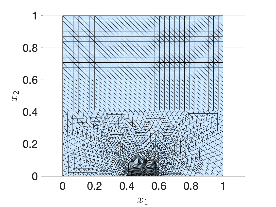
(b)

Figure 1: geometric configuration: (a) the non-dimensional domain (b) the mesh. The size of each alveoulus is equal to $l_{Q}=3.09\,[\rm m]$, while the distance between consecutive alveoli is equal to $l=6.18\,[\rm m].$

The grid is refined in the proximity of the alveoli to better capture the relevant features of the solution. We consider a $\texttt{p}=3$ FE discretisation for the displacement component, and a $\texttt{p}=2$ FE discretisation for both pressure and temperature.

4.2 Mathematical problem

We first state the equilibrium equations – the superscripts $(\cdot)^{\rm{m}}$, $(\cdot)^{\rm{n}}$,$(\cdot)^{\rm{t}}$ refer to quantities associated with the mechanical, hydraulic and thermal behaviours, respectively. Then, we present the constitutive laws that are considered and finally we present the boundary conditions. To clarify the presentation, we report in Table 4 the parameters that enter in the constitutive laws.

We denote by $\underline{F}_{\rm{m}}=-\frac{g}{\gamma}\underline{e}_{2}$ (where $\gamma=\frac{\sigma_{0}}{\rho_{0}\bar{H}}$) the mechanical force with $g$ defined in Table 4 and we specify that $\underline{n}$ (resp. $\underline{t}$) is the unitary outward normal (resp. tangential) vector in the domain depicted in Figure 1LABEL:sub@fig:domain; then we introduce the equilibrium of mechanical forces:

$$\left\{\begin{array}[]{ll}-\nabla\cdot\underline{\underline{\sigma}}\,=\,\rho\underline{F}_{\rm m}&{\rm in}\,\Omega,\\[8.53581pt] \underline{\underline{\sigma}}\,\underline{n}=\underline{g}_{\rm m,N}&{\rm on}\,\Gamma_{\rm N},\\[8.53581pt] \underline{u}\cdot\underline{n}=0&{\rm on}\,\partial\Omega\setminus\Gamma_{\rm N},\\[8.53581pt] (\underline{\underline{\sigma}}\,\underline{n})\cdot\underline{t}=0&{\rm on}\,\partial\Omega\setminus\Gamma_{\rm N},\end{array}\right.$$ (23a)

where $$\Gamma_{\rm N} \underline{g}_{\rm m,N} \underline{g}_{\rm m,N}=-\underline{e}_{2}$$ is depicted in Figure  1LABEL:sub@fig:domain. The Neumann datum is given by . The stress tensor is linked to the primary and internal variables by the linear law

$$\underline{\underline{\sigma}}=2{\mu}{\nabla}_{\rm s}{\underline{u}}+\left({\lambda}\,{\nabla}\cdot{\underline{u}}\,-\,(2{\mu}+3{\lambda}){\alpha_{\rm s}}{T}-b{p}_{\rm w}\right)\mathbbm{1},$$ (23b)

where the Lamé constants $\mu^{\prime},\,\lambda$ satisfy

$$\mu^{\prime}=\frac{E}{2(1+\nu)},$$

$$\lambda=\frac{E\nu}{(1+\nu)(1-2\nu)},$$

and $E$ and $\nu$ are introduced in Table 4.

We state the mass conservation of water as follows

$$\left\{\begin{array}[]{ll}\partial_{{t}}\,{m}_{\rm w}\,+\,{\nabla}\cdot{\underline{M}}_{\rm w}=0&{\rm in}\,\Omega\\[8.53581pt] {\underline{M}}_{\rm w}\cdot\underline{n}=0&{\rm on}\,\partial\Omega\\ \end{array}\right.$$ (24a)

where the muss flux $$\underline{M}_{\rm{w}}$$ is given by the Darcy law

$${{\underline{M}}_{\rm w}=-{\gamma}\left({\nabla}{p}_{\rm w}-{\rho}_{\rm w}{\underline{F}}_{\rm m}\right)},$$ (24b)

and

$${{\gamma}=\rho_{\rm{w}}\frac{\kappa_{\rm w}\,\sigma_{0}\,\bar{t}}{\rho_{0}\mu_{\rm w,0}\,\bar{H}^{2}}\,{\rm exp}\left(-\frac{1808.5}{T_{\rm ref}+\overline{\Delta T}\,{T}}\right)}.$$ (24c)

Finally we consider the energy balance:

$$\left\{\begin{array}[]{ll}{h}_{\rm w}\partial_{{t}}\,{m}_{\rm w}\,+\,\partial_{{t}}\,{\mathcal{Q}}\,+\,{\nabla}\cdot\left({h}_{\rm w}{\underline{M}}_{\rm w}\,+\,{\underline{q}}\right)-{\underline{M}}_{\rm w}\cdot{\underline{F}}_{\rm m}\,=\,{\Theta}&{\rm in}\,\Omega\\[8.53581pt] \left({h}_{\rm w}{\underline{M}}_{\rm w}\,+\,{\underline{q}}\right)\cdot\underline{n}={g}_{\rm t,N}&{\rm on}\,\partial\Omega\\ \end{array}\right.$$ (25a)

where $$\mathcal{Q} \underline{q}$$ is the non-convective heat, is the thermal flux and is given by the Fick law

$${{\underline{q}}=-{\Lambda}{\nabla}{T},}$$ (25b)

with $${\Lambda}=\rm{diag}({\lambda}_{1},{\lambda}_{2})$$.

If we denote by $\Gamma_{\rm{al}}\subset\partial\Omega$ the region associated with the alveoli, $g_{t,N}$ is equal to

$$g_{t,N}=\frac{P_{\rm{t}}n_{c}\bar{t}}{l_{Q}\bar{H}^{2}\sigma_{0}}\exp\big{(}-t/\tau\big{)}\mathbbm{1}_{\Gamma_{\rm al}}=C_{\rm{al}}\exp\big{(}-t/\tau\big{)}\mathbbm{1}_{\Gamma_{\rm{al}}},$$ (26)

where $n_{c}\,[\%]$ is the density of the radioactive waste stock in each alveolus (equal to $45$ anisters), $P_{\rm{t}}=31.4\,[\rm{W}]$ is the unitary termic power at the initial time, $l_{Q}=3.09\,[\rm{m}]$ is the size of each alveolus, $\sigma_{0},\bar{H},\bar{t}$ are introduced in Table 3 and $\tau=\frac{\bar{t}}{\log(0.112)}\,[\rm{s}]$ is a characteristic decay time.

$$\displaystyle{\frac{d\rho_{\rm w}}{\rho_{\rm w}}\,=\,\frac{dp_{\rm w}}{K_{\rm w}}\,-\,3{\alpha}_{\rm w}dT}$$ (27a)

$$\displaystyle{\frac{d\varphi}{b\,-\,\varphi}\,=\,d\epsilon_{\rm V}\,-3{\alpha}_{\rm s}d{T}+\frac{d{p}_{\rm w}}{{K}_{\rm s}}},$$ (27b)

$$\displaystyle{d{h}_{\rm w}={C}_{\rm w}^{\rm p}\,d{T}\,+\,(\beta_{h}^{\rm p}-3{\alpha}_{\rm w}{T})\frac{d{p}_{\rm w}}{{\rho}_{\rm w}}},$$ (27c)

$$\displaystyle{\delta{\mathcal{Q}}=\left(\beta_{\mathcal{Q}}^{\epsilon}+3{\alpha_{\rm s}}{K}_{0}\,{T}\right)\,d\epsilon_{\rm V}\,-\left(\beta_{\mathcal{Q}}^{\rm p}+3{\alpha}_{\rm w,m}{T}\right)\,d{p}_{\rm w}\,+\,{C}_{\epsilon}^{0}\,d{T}},$$ (27d)

$$\displaystyle{{m}_{\rm w}={\rho}_{\rm w}(1+\epsilon_{\rm V})\,\varphi-{\rho}_{\rm w}^{0}\varphi^{0}}$$ (27e)

Here, we have $\beta_{h}^{p}=1-3\alpha_{\rm{w}}T_{\rm ref}$, $\beta_{\mathcal{Q}}^{\epsilon}=3\alpha_{\rm s}K_{0}T_{\rm ref}$, $\beta_{\mathcal{Q}}^{p}=3\alpha_{\rm w,m}T_{\rm{ref}}$.
The parameters in (27a)-(27e) are defined in Table 4.

	SI unit	description	reference value	formula
$g$	$\rm m\cdot s^{-2}$	gravity acceleration	$9.81$
$E$	$\rm Pa$	Young’s modulus	$11.4\cdot 10^{9}\>\rm UA$ $12.3\cdot 10^{9}\>{\rm UT}$ $20\cdot 10^{9}\>{\rm USC}$
$\nu$	$\%$	Poisson’s ratio	$0.3$
$\mu$	$\rm Pa$	Lamé parameter,		$\frac{E}{2(1+\nu)}$
$\lambda$	$\rm Pa$	Lamé parameter		$\frac{E\nu}{(1+\nu)(1-2\nu)}$
$b$	$\%$	Biot coefficient	$0.6$
$\alpha_{\rm s}$	$\rm K^{-1}$	solid thermal expansion coefficient	$1.28\cdot 10^{-5}$
$\alpha_{\rm 0}$	$\rm K^{-1}$	expansion coefficient	$1.28\cdot 10^{-5}$
$\kappa_{\rm w}$	$\rm m^{2}$	intrinsic permeability of porous medium	$10^{-21}$
$\mu_{\rm w}$	$\rm MPa\cdot s$	dynamic viscosity		$\mu_{\rm w}=\mu_{\rm w,0}\exp(\frac{1808.5}{T})$
$\mu_{\rm w,0}$	$\rm MPa\cdot s$	dynamic viscosity coefficient	$2.1\cdot 10^{-12}$
$K_{\rm s}$	$\rm Pa$	bulk modulus of the solid
$K_{\rm{w}}$	$\rm Pa$	bulk modulus of water	$2\cdot 10^{9}$	$K_{\rm s}=\frac{E}{3(1-2\nu)}$
$C_{\rm w}^{\rm p}$	$\rm J\cdot kg^{-1}\cdot K^{-1}$	heat capacity at constant pressure	$4180$
$K_{0}$	$\rm Pa$	drained bulk modulus		$K_{0}=(1-b)K_{\rm s}$
$\alpha_{\rm{w}}$	$K^{-1}$	thermal expansion coefficient of water		$\alpha_{\rm{w}}=9.52\cdot 10^{-5}\log(T-273)-2.19\cdot 10^{-4}$
$\alpha_{\rm w,m}$		dilation coefficient
$C_{\sigma}^{\rm s}$	$\rm J\;kg^{-1}\cdot K$	specific heat at constant stress	$537\>{\rm UA}$ $603\>{\rm UT}$ $640\>{\rm USC}$
$\rho^{0}$	$\rm Kg\cdot m^{-3}$	porous medium initial density	$2450\>{\rm UA}$ $2450\>{\rm UT}$ $2500\>{\rm USC}$
$\rho_{\rm{w}}^{0}$	$\rm Kg\cdot m^{-3}$	initial water density	$10^{3}$
$\varphi^{0}$	$\%$	initial Eulerian porosity	$0.25\>{\rm UA}$ $0.21\>{\rm UT}$ $0.19\>{\rm USC}$
$h_{\rm w}^{0}$	$\rm m^{2}\cdot s^{-2}$	initial water enthalpy		$h_{\rm w}^{0}=\frac{p_{\rm w}^{0}-p_{\rm atm}}{\rho_{\rm w}^{0}}$
$\rho_{\rm s}$	$\rm Kg\cdot m^{-3}$	density ratio		$\rho_{\rm s}=\frac{\rho^{0}-\rho_{\rm w}^{0}\varphi^{0}}{1-\varphi^{0}}$
$C_{\epsilon}^{0}$	$\rm Pa\cdot K^{-1}$	specific heat at constant deformation		$C_{\epsilon}^{0}=(1-\varphi)\rho_{s}C_{\sigma}^{s}+\varphi\rho_{w}C_{w}^{p}-9TK_{0}\alpha_{\rm s}^{2}$
$\Lambda$		thermic conductivity tensor		$\Lambda=\rm{diag}(\lambda_{1},\lambda_{2})$
$\lambda_{1}$	$\rm Wm^{-1}K^{-1}$	thermic conductivity component	$\begin{array}[]{ll}1.5&{\rm UA}\\ 1.5&{\rm UT}\\ 1.3&{\rm USC}\\ \end{array}$
$\lambda_{2}$	$\rm Wm^{-1}K^{-1}$	thermic conductivity component	$\begin{array}[]{ll}1&{\rm UA}\\ 1&{\rm UT}\\ 1.3&{\rm USC}\\ \end{array}$
$\Theta$	$\rm Pa\cdot s^{-1}$	volumetric heat sources

Table 4: parameters of the constitutive laws. Layers UA, UT, USC are depicted in Figure 1 LABEL:sub@fig:domain.

4.2.1 Initial conditions

To set the initial conditions, we consider the case of deactivated repositories: therefore, we set thermal flux equal to zero and we set a constant temperature $T_{0}=T_{\rm{ref}}$ in $\Omega$, where the reference temperature is defined in Table 3. We aim at finding the initial values of the primary variables $\underline{u}$ and $p_{\rm{w}}$ that correspond to the equilibium solutions of a preliminary problem: here, the Neumann boundary condition for the energy equation is zero, that is, $g_{\rm t,N}=0$, and temperature is costant and equal to the reference value $T_{\rm{ref}}$ (in Table 3).
We then seek $\underline{u}_{0}$, $p_{\rm{w},0}$ such that the initial solution vector $\underline{U}_{0}=[\underline{u}^{\rm{T}}_{0},p_{\rm{w}},T_{0}]^{\rm{T}}$ satisfies the equilibrium equations (23a), (24a) and (25a) with thermal flux $g_{\rm{t,N}}$ equal to $0$ on the domain boundary $\partial\Omega$. Towards this end, we first observe that (27a) reduces to

$$\frac{d\rho_{\rm{w}}}{\rho_{\rm{w}}}=\frac{dp_{\rm{w}}}{K_{\rm{w}}}$$ (28)

that brings to $p_{\rm{w}}=\rho_{-\infty}\exp\left(\frac{1}{K_{\rm{w}}}(p_{\rm{w}}-p_{-\infty})\right)$. If we assume that $\rho_{\rm{w}}=\rho_{-\infty}=\rho_{\rm{w},0}$, we find $p_{\rm{w}}=p_{-\infty}$; furthermore, by susbstituting these assumptions into the hydraulic equilibrium equation we find

$$p_{\rm{w},0}(x,y)=p_{\rm{w,top}}+\rho_{\rm{w},0}g(1-y)$$ (29)

where $p_{\rm{w,top}}$ is a datum for water pressure that is defined at the top boundary of the domain $(0,1)\times\{1\}$. Finally, we search for $\underline{u}_{0}$ as the solution to the equilibrium equation of mechanical forces:

$$\int_{\Omega}\,2\mu\,\nabla_{\rm s}\,\underline{u}_{0}\,:\,\nabla_{\rm s}\,\underline{v}\,+\,\lambda(\nabla\cdot\underline{u}_{0})(\nabla\cdot\underline{v})-bp_{\rm{w},0}\,\nabla\cdot\underline{v}\,-\,{\rho}^{0}\underline{F}_{\rm m}\cdot\underline{v}\,dx=\int_{\Gamma_{\rm N}}\,{\underline{g}}_{\rm m,N}\cdot\underline{v}\,dx,$$ (30)

for all $\underline{v}\in\mathcal{X}^{\rm u}_{\rm{hf}}$, such that $\underline{v}\cdot\underline{n}|_{\partial\Omega\setminus\Gamma_{\rm N}}=0$.

4.3 Finite element formulation

We resort to an implicit Euler time discretisation scheme, with $J_{\rm{max}}=100$ uniform time steps; the superscript $(\cdot)^{+}$ refers to the new solution (at the current time step $j$, for $j=1,...,J_{\rm{max}}$), while $(\cdot)^{-}$ refers to the solution at the previous time steps:

$$\left\{\begin{array}[]{l}\displaystyle{\int_{\Omega}\,2{\mu}\,\nabla_{\rm s}\,\underline{u}^{+}\,:\,\nabla_{\rm s}\,\underline{v}\,+\,\left(\lambda\nabla\cdot\underline{u}^{+}\,-\,(2{\mu}+3{\lambda})\,{\alpha}_{\rm s}T^{+}-b{p}^{+}_{\rm w}\right)\,\nabla\cdot\underline{v}\,-\,\left({\rho}^{0}+m^{+}_{\rm w}\right)\,{\underline{F}}_{\rm m}\cdot\underline{v}\,dx}\\[5.69054pt] \displaystyle{\hskip 216.81pt=\,\int_{\Gamma_{\rm N}}\,\underline{g}^{+}_{\rm m,N}\cdot\mathbf{v}\,dx;}\\[8.53581pt] \displaystyle{\int_{\Omega}\,\frac{1}{\Delta t}(m^{+}_{\rm w}-m^{-}_{\rm{w}})\,\psi\,+\,{\gamma^{+}}\,(\nabla{p}^{+}_{\rm w}-\rho^{+}_{\rm w}\underline{F}_{\rm m})\cdot\nabla\psi\,dx\,=0;}\\[8.53581pt] \displaystyle{\int_{\Omega}\,\Big{(}\left(\frac{{h}_{\rm w}}{\Delta t}(m^{+}_{\rm w}-m^{-}_{\rm{w}})\,+\,\frac{1}{\Delta t}(\mathcal{Q}^{+}-\mathcal{Q}^{-})\,+\,\gamma^{+}\,(\nabla{p}^{+}_{\rm w}-\rho^{+}_{\rm w}\underline{F}_{\rm m})\cdot\underline{F}_{\rm m}\right)\,\xi\,-\,\left(-\,h^{-}_{\rm w}\,(\nabla p^{+}_{\rm w}-\rho^{+}_{\rm w}{\underline{F}}_{\rm m})\,+\,{\underline{q}}\right)\,\cdot\nabla\xi}\\[5.69054pt] \displaystyle{\hskip 216.81pt\,=\,\int_{\Omega}\,\Theta^{+}\,\xi\,dx\,-\,\int_{\partial\Omega}\,\ g^{+}_{\rm t,N}\,\xi\,dx;}\\ \end{array}\right.$$ (31)

for all $\underline{v}\in\mathcal{X}^{\rm u}_{\rm{hf}}$ such that $\underline{v}\cdot\underline{n}|_{\partial\Omega\setminus\Gamma_{N}}=0$, $\psi\in\mathcal{X}^{\rm p}_{\rm{hf}}$, $\xi\in\mathcal{X}^{\rm t}_{\rm{hf}}$, where

$$\left\{\begin{array}[]{l}\displaystyle{\rho_{\rm w}^{+}\,=\,\rho_{\rm w}^{-}\,{\rm exp}\left(\frac{p_{\rm w}^{+}-p_{\rm w}^{-}}{K_{\rm w}}\,-\,3\alpha_{\rm w}(T^{+}-T^{-})\right);}\\[8.53581pt] \displaystyle{\varphi^{+}=b\,-\,(b-\varphi^{-})\,{\rm exp}\left(-(\epsilon_{\rm V}^{+}-\epsilon_{\rm V}^{-})+3\alpha_{0}(T^{+}-T^{-})\,-\frac{1}{K_{s}}\,(p_{\rm w}^{+}-p_{\rm w}^{-})\right);}\\[8.53581pt] \displaystyle{h_{\rm w}^{+}=h_{\rm w}^{-}\,+\,C_{\rm w}^{\rm p}\,(T^{+}-T^{-})\,+\,\frac{\beta_{h}^{\rm p}-3\alpha_{\rm w}T^{+}}{\rho_{\rm w}^{+}}\left(p_{\rm w}^{+}-p_{\rm w}^{-}\right);}\\[8.53581pt] \displaystyle{\mathcal{Q}^{+}=\mathcal{Q}^{-}\,+\,\left(\beta_{\mathcal{Q}}^{\epsilon}+3\alpha_{\rm s}K_{0}\,\frac{1}{2}(T^{+}+T^{-})\right)\,\left(\epsilon_{\rm V}^{+}-\epsilon_{\rm V}^{-}\right)\,-\left(\beta_{\mathcal{Q}}^{\rm p}+3\alpha_{\rm w,m}^{+}\frac{1}{2}(T^{+}+T^{-})\right)\,\left(p_{\rm w}^{+}\,-\,p_{\rm w}^{-}\right)}\\ \displaystyle{\hskip 216.81pt\,+\,C_{\epsilon}^{0,+}\,(T^{+}-T^{-});}\\[8.53581pt] \displaystyle{m_{\rm w}^{+}=\rho_{\rm w}^{+}(1+\epsilon_{\rm V}^{+})\,\varphi^{+}-\rho_{\rm w}^{0}\,\varphi^{0}.}\end{array}\right.$$ (32)

4.4 Choice of the norm

We equip the FE space $\mathcal{X}_{\rm{hf}}$ with the weighted inner product

$$(\underline{U},\underline{U}^{\prime})=\frac{1}{\lambda_{\rm{u}}}\sum_{d=1}^{2}(\underline{u}_{d},\underline{u}^{\prime}_{d})_{H^{1}(\Omega)}+\frac{1}{\lambda_{\rm{p}}}(p,p^{\prime})_{H^{1}(\Omega)}+\frac{1}{\lambda_{\rm{t}}}(T,T^{\prime})_{H^{1}(\Omega)},$$ (33)

where the coefficients $\lambda_{\rm{u}},\lambda_{\rm{p}},\lambda_{\rm{t}}$ are the largest eigenvalues of the Gramian matrices $\mathbf{C}^{\rm{u}}$, $\mathbf{C}^{\rm{p}}$, $\mathbf{C}^{\rm{t}}$ associated to displacement, pressure and temperature, respectively. Similarly to [28], the inner product (33) is motivated by the need for properly taking into account the contributions of displacement, pressure and temperature, which are characterised by different magnitudes and different units.

4.5 Parametrization

We consider a vector of four parameters: the Young’s modulus $E$ and the Poisson’s ratio $\nu$ in the region UA, the thermic factor $\tau$ and the constant $C_{\rm{al}}$ in (26). For all parameters, we define the parameter domain $\mathcal{P}$ by considering variations of $\pm 15\%$ with respect to the nominal value reported in Table 4.

5 Numerical results

We measure performance through the discrete $L^{2}(0,T_{\rm{f}};\mathcal{X}_{\rm{hf}})$ relative error

$$E_{\mu}:=\frac{\sqrt{\displaystyle{\sum_{j=1}^{J_{\rm{max}}}}{\left(t^{(j)}-t^{(j-1)}\right)\big{\|}\underline{U}^{(j)}_{\rm{hf},\mu}-\widehat{\underline{U}}^{(j)}_{\mu}\big{\|}^{2}}}}{\sqrt{\displaystyle{\sum_{j=1}^{J_{\rm{max}}}}{\left(t^{(j)}-t^{(j-1)}\right)\|\underline{U}^{(j)}_{\rm{hf},\mu}\|^{2}}}}$$ (34)

for any $\mu\in\mathcal{P}$. Similarly, we denote by $E^{\rm{u}}_{\mu}$, $E^{\rm{p}}_{\mu}$ and $E^{\rm{t}}_{\mu}$ the discrete relative $L^{2}(0,T_{\rm{f}};\mathcal{X}_{\rm{hf}})$ errors associated with the estimate of displacement, pressure and temperature, respectively.

5.1 Solution reproduction problem

We first present numerical results for a fixed configuration of parameters $\bar{\mu}\in\mathcal{P}$ to validate the ROM described in section 3. We consider $\bar{\mu}$ equal to the centroid of $\mathcal{P}$. We perform data compression based on the whole set of snapshots, i.e. $|I_{\rm{s}}|=J_{\rm{max}}=100$.

5.1.1 Data compression: POD

In Figure 2 we compare performance of the global POD based on the weighted inner product $(\cdot,\cdot)$ with the performance of the component-wise POD. More precisely, we define $\underline{Z}$ such that

$$[\underline{Z},\boldsymbol{\lambda}]=\texttt{POD}\left(\{\underline{U}_{\rm hf,\bar{\mu}}^{(j)}\}_{j\in I_{\rm{s}}},(\cdot,\cdot),tol_{\rm pod}\right),$$ (35)

and we extract the displacement, pressure and temperature components $\underline{Z}^{\rm{u}}$, $\underline{Z}^{\rm{p}}$, $\underline{Z}^{\rm{t}}$. Then , we denote the ”optimal” (in a discrete $L^{2}$ sense) spaces

$$[\underline{Z}^{u,\rm{opt}},\boldsymbol{\lambda}^{u,\rm{opt}}]=\texttt{POD}\left(\{\underline{u}_{\rm hf,\bar{\mu}}^{(j)}\}_{j\in\texttt{I}_{\rm{s}}},(\cdot,\cdot)_{H^{1}},tol_{\rm pod}\right);$$ (36)

$$[\underline{Z}^{p,\rm{opt}},\boldsymbol{\lambda}^{p,\rm{opt}}]=\texttt{POD}\left(\{p_{\rm hf,\bar{\mu}}^{(j)}\}_{j\in\texttt{I}_{\rm{s}}},(\cdot,\cdot)_{H^{1}},tol_{\rm pod}\right);$$ (37)

$$[\underline{Z}^{T,\rm{opt}},\boldsymbol{\lambda}^{T,\rm{opt}}]=\texttt{POD}\left(\{T_{\rm hf,\bar{\mu}}^{(j)}\}_{j\in\texttt{I}_{\rm{s}}},(\cdot,\cdot)_{H^{1}},tol_{\rm pod}\right).$$ (38)

In Figure 2 LABEL:sub@fig:eigenvalues we show the behaviour of the POD eigenvalues in (35); in Figure 2LABEL:sub@fig:proj-u, LABEL:sub@fig:proj-p, LABEL:sub@fig:proj-T we compare the relative projection errors associated with $\underline{Z}^{\rm{u}}$ and $\underline{Z}^{\rm{u,opt}}$, $\underline{Z}^{\rm{p}}$, $\underline{Z}^{\rm{p,opt}}$ and $\underline{Z}^{\rm{t}}$ and $\underline{Z}^{\rm{t,opt}}$. We observe that the projection errors are nearly the same for all the three state variables: this obervation suggests to consider a single reduced space to approximate the solution field.

(a) POD eigenvalues

(b) Projection errors: $\underline{u}$

(c) Projection errors: $p_{\rm{w}}$

(d) Projection errors: $T$

Figure 2: LABEL:sub@fig:eigenvalues: exponential decay of POD eigenvalues. LABEL:sub@fig:proj-u, LABEL:sub@fig:proj-p, LABEL:sub@fig:proj-T: projection errors computed through (35) (in black) and (36)-(38)(in red) for increasing numbers of POD modes.

5.1.2 Hyper-reduction

In Figure 3LABEL:sub@fig:hyper_errors we show the performance of the Galerkin ROM with and without hyper-reduction. We distinguish between the high-fidelity quadrature rule, abbreviated as $\rm{hfq}$, and the empirical quadrature rule for several tolerances $tol_{\rm{eq}}$. We also add as a reference, the relative projection error. Figure 3LABEL:sub@fig:elements shows the percentage of selected elements $\frac{\rm{Q}}{N_{\rm{e}}}\times 100\%$ for the same choices of the tolerance $tol_{\rm{eq}}$. We observe that the empirical quadrature procedure is able to significantly reduce the size of the mesh used for online calculations without compromising accuracy. The plateau for $N\gtrsim 14$ is due to the tolerance of the Newton iterative solver.

(a) Errors

(b) Selected elements

Figure 3: solution reproduction problem. LABEL:sub@fig:hyper_errors: errors associated to projection error (proj), Galerkin with high-fidelity quadrature (hfq) and Galerkin with empirical quadrature for several choices of $tol_{\rm{eq}}$ with respect to the ROM dimension $N$. LABEL:sub@fig:elements: percentage of selected elements for several $tol_{\rm{eq}}$.

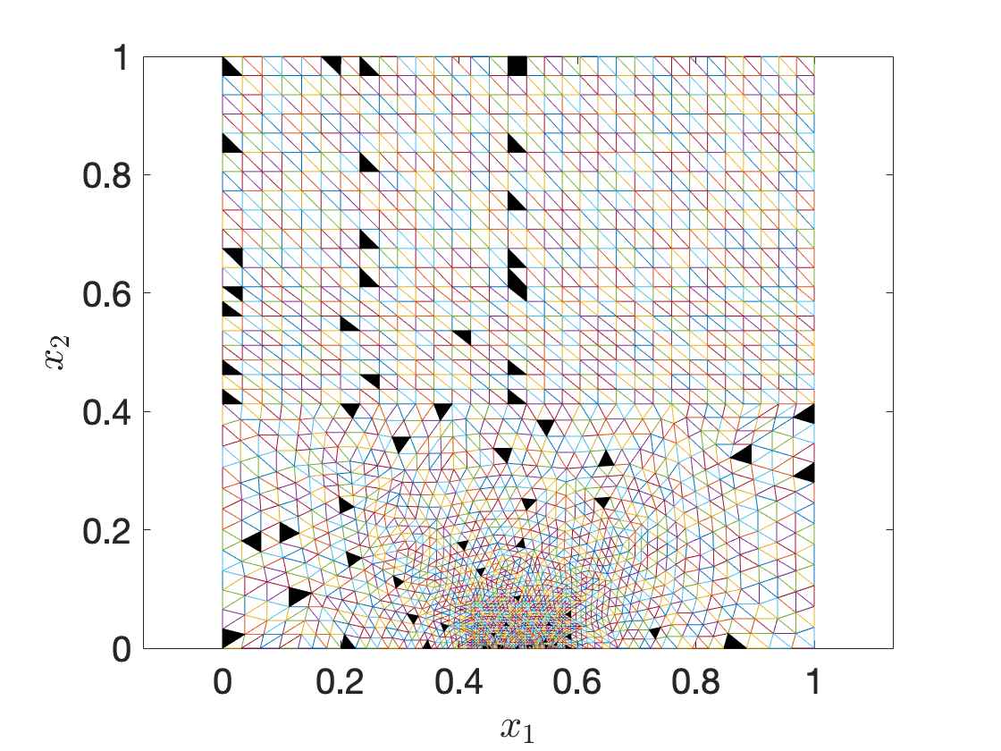
(a) $tol_{\rm{eq}}=10^{-14}$

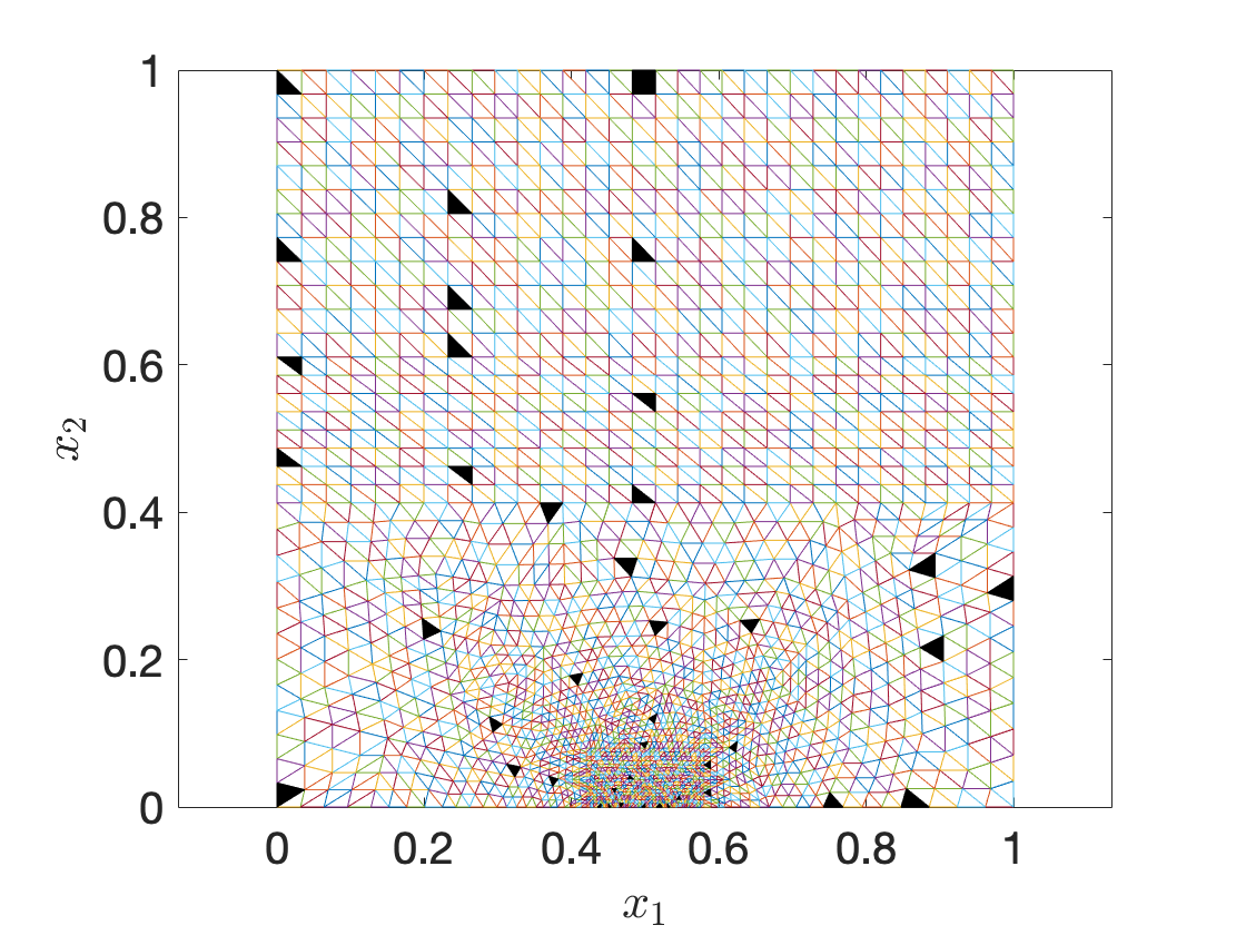
(b) $tol_{\rm{eq}}=10^{-10}$

Figure 4: solution reproduction problem. Reduced mesh for two choices of the empirical quadrature tolerance.

In Figure 4, we show the selected grid elements for two choices of the EQ tolerance value $tol_{\rm{eq}}$ and for $N=12$. We observe that the sampled elements are distributed over the whole domain with a slight prevalence of elements in the proximity of the alveoli.

5.2 Parametric problem

We present results for the parametric case. We denote by $\Xi_{\rm{train}}\subset\mathcal{P}$ the training set used to build the ROM and by $\Xi_{\rm test}\subset\mathcal{P}$ the test set used to assess performance. Both sets consist of independent identically distributed samples of a uniform distribution in $\mathcal{P}$, with $|\Xi_{\rm{train}}|=n_{\rm{train}}=50$ and $|\Xi_{\rm test}|=n_{\rm{test}}=10$. We also set $tol_{\rm{POD}}=10^{-7}$ in (8) and in (13b) for data compression, and we set $tol_{\rm POD,res}=10^{-5}$ in (8) for the construction of the empirical test space. We set $I_{\rm s}\subset\{1,...,J_{\rm{max}}\}$ with $|I_{\rm s}|=20$. EQ rules are depicted usign the tolerance $tol_{\rm{eq}}=10^{-12}$ (cf . Algorithm 4).

5.2.1 Error estimation

In Figure 5 we compare the dual residual and several EQ errors for each parameter $\mu$ in the training set $\Xi_{\rm train}$ and for different dimensions of the reduced space that is progressively updated during the execution of the POD-Greedy algorithm. In particular, we show results in two cases: the hierarchical POD-Greedy (H-POD) and the hierarchical approximate POD-Greedy (denoted as HA-POD). Figures 5LABEL:sub@fig:HPOD_correlation and 5LABEL:sub@fig:HAPOD_correlation show for both H-POD and HA-POD to what extent the residual-based error indicator defined in (17) is correlated with the relative error (34). We observe that for values of the indicators that are larger than $10^{-3}$, correlation is very high, while for smaller values correlation is much weaker.

(a) H-POD

(b) HA-POD

Figure 5: parametric problem: correlation between the time-average residual indicator (17) and true relative errors (34).

To provide a a concrete reference, in Figure 6 we investigate the correlation between the relative error (34) and the time-discrete $L^{2}(0,T_{\rm{f}};\mathcal{X}^{\prime}_{\rm{hf},0})$ residual indicator defined in (21): we observe that the indicator in (21) is significantly more accurate, particularly for small values of the error. As stated in section 3, the residual indicator (21) is considerably more expensive in terms of both memory and computational costs.

Figure 6: parametric problem: correlation between residual indicator (21) and true relative errors 34.

5.2.2 POD-Greedy sampling

In Figures 7 and 8 we show the POD-Greedy algorithm convergence history, for both the hierarchical and approximate hierarchical PODs. At each iteration of the algorithm, until convergence, the error indicator $\Delta_{\mu}$ is illustrated with respect to training parameter indices $\mathcal{I}_{\rm{train}}=\{1,...,|\Xi_{\rm{train}}|\}$ . At each iteration the selected parameter $\mu^{\star}$ is marked in red, while the previously selected parameters are marked in green. We also report the dimension of the updated reduced space and the number of sampled elements.

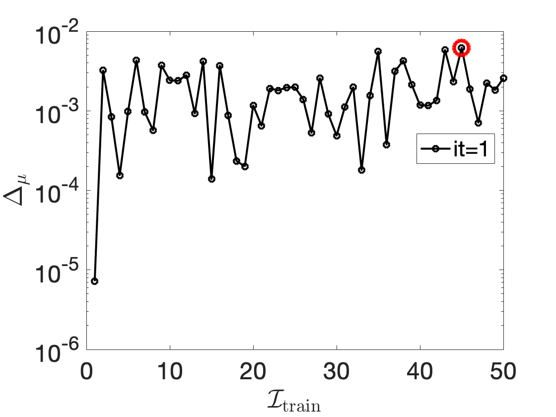
(a) Iteration $\rm{it}=1$; $N=15$, $Q=74$, $Q_{\rm r}=16$

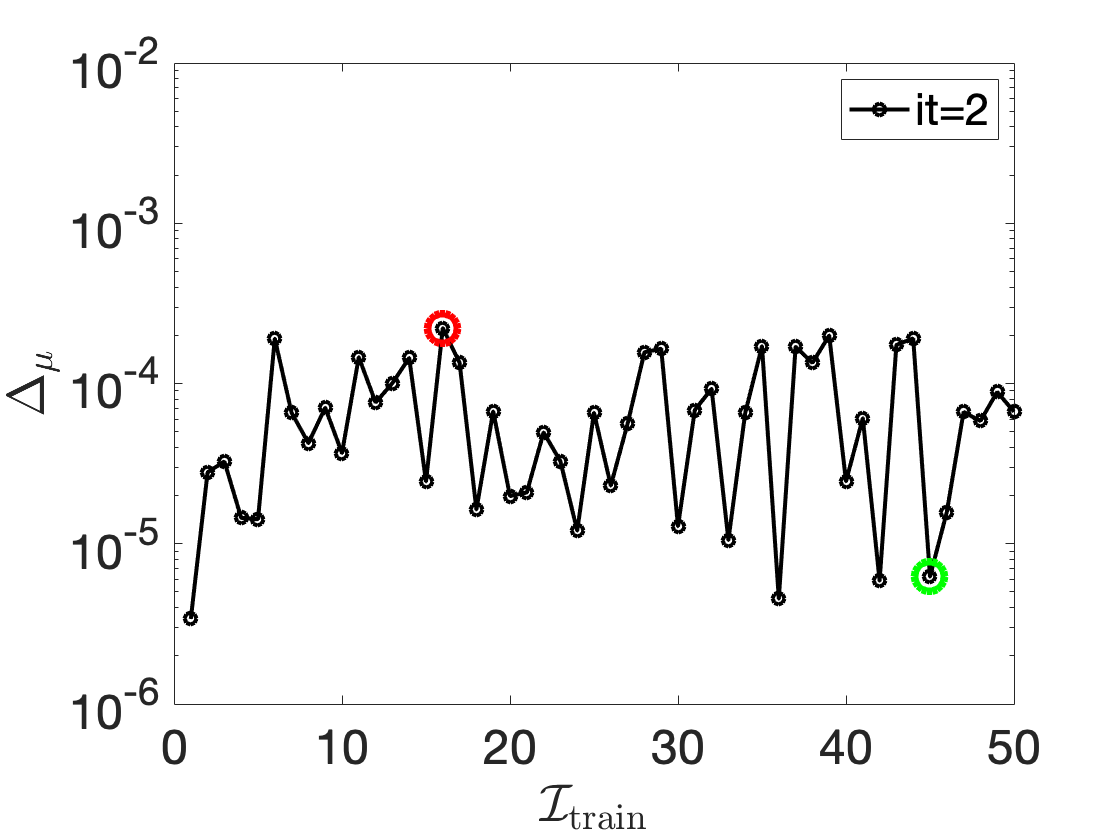
(b) Iteration $\rm{it}=2$; $N=26$, $Q=123$, $Q_{\rm r}=18$

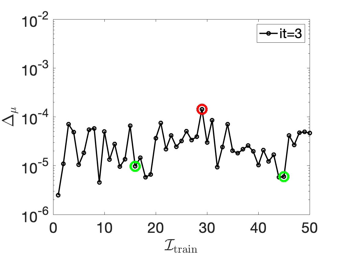
(c) Iteration $\rm{it}=3$; $N=35$, $Q=155$, $Q_{\rm r}=22$

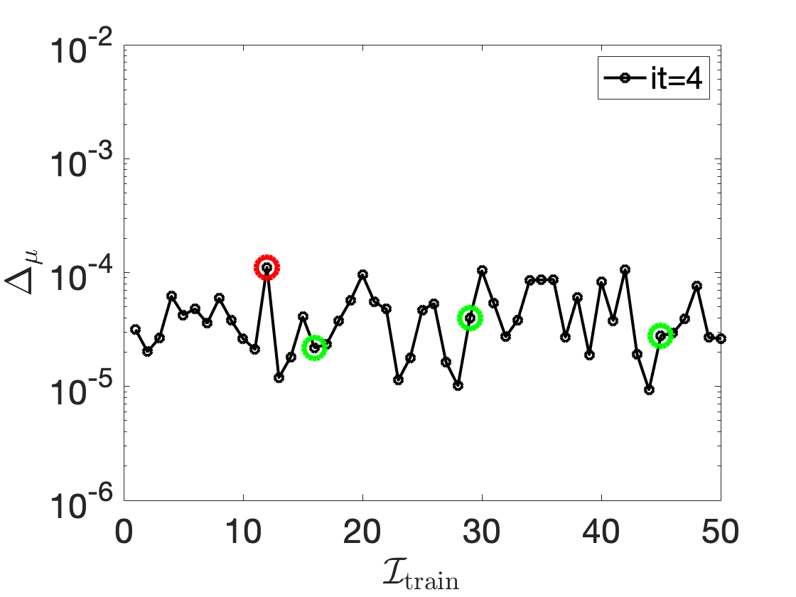
(d) Iteration $\rm{it}=4$; $N=43$, $Q=169$, $Q_{\rm r}=18$

Figure 7: parametric problem: POD-Greedy algorithm convergence history in the H-POD case.

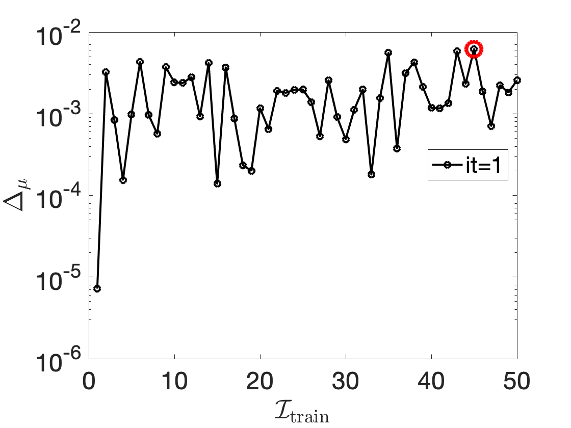
(a) $\rm{it}=1$; $N=15$,$Q=74$,$Q_{\rm r}=16$

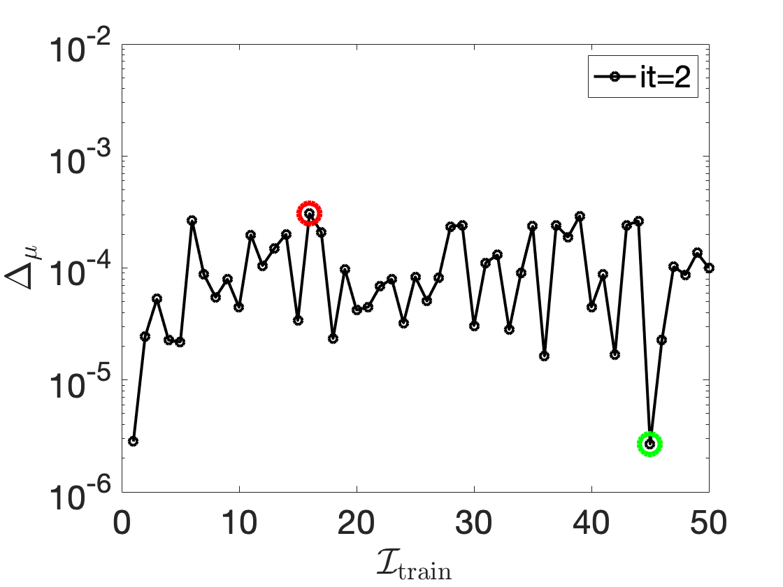
(b) $\rm{it}=2$; $N=25$,$Q=120$, $Q_{\rm r}=19$

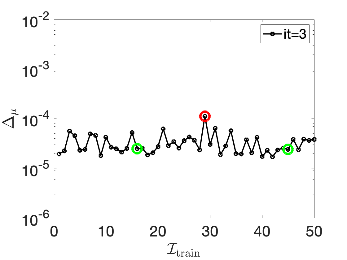
(c) $\rm{it}=3$; $N=31$,$Q=135$, $Q_{\rm r}=21$

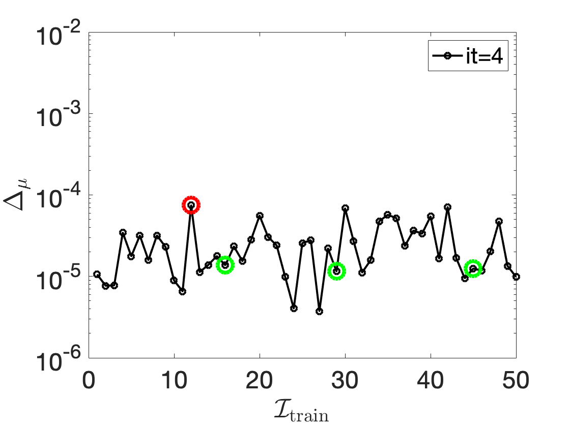
(d) Iteration $\rm{it}=4$; $N=37$,$Q=156$, $Q_{\rm r}=19$

Figure 8: parametric problem: POD-Greedy algorithm convergence history in the HA-POD case.

5.2.3 Predictive tests

In Figure 9, we assess out-of-sample performance of the proposed method. More precisely, we show the behaviour of the maximum relative error (34) over the test set $\displaystyle\max_{\mu\in\Xi_{\rm test}}E_{\mu}$ for both H-POD Greedy and HA-POD Greedy. To provide a relevant benchmark, we compare results with the H-POD Greedy and HA-POD Greedy algorithms based on the exact errors (strong POD-Greedy). For this particular example, we observe that the proposed method is effective to generate accurate ROMs: in particular, the Greedy procedures based on the time-averaged error indicator are comparable in terms of performance with the corresponding strong POD-Greedy algorithms.

(a) H-POD Greedy

(b) HA-POD Greedy

Figure 9: Out-of-sample performance of the ROM parametric problem obtained using the POD-Greedy algorithm. Comparison with strong POD Greedy.

6 Conclusions

In this work, we developed and numerically validated a model order reduction procedure for a class of problems in nonlinear mechanics, and we successfully applied it to a two-dimensional parametric THM problems that arises in radio-active waste management. We proposed a time-averaged error indicator to drive the offline Greedy sampling, and an empirical quadrature procedure to reduce offline costs.

We aim to extend the approach in several directions. First, we wish to apply our method to other problems of the form (1), to demonstrate the generality of the approach and its relevance for continuum mechanics applications. Second, we wish to combine our approach with domain decomposition methods ([3, 18, 17]) to deal with more complex parametrizations and topological changes. Towards this end, we wish to devise effective localised training methods to reduce offline costs and domain decomposition strategies to glue together the solution in different components of the domain.

References

• [1] M. Barrault, Y. Maday, N. C. Nguyen, and A. T. Patera. An empirical interpolation method: application to efficient reduced-basis discretization of partial differential equations. Comptes Rendus Mathematique, 339(9):667–672, 2004.
• [2] M. Bergmann, C.-H. Bruneau, and A. Iollo. Enablers for robust POD models. Journal of Computational Physics, 228(2):516–538, 2009.
• [3] M. Bergmann, A. Ferrero, A. Iollo, E. Lombardi, A. Scardigli, and H. Telib. A zonal Galerkin-free POD model for incompressible flows. Journal of Computational Physics, 352:301–325, 2018.
• [4] G. Berkooz, P. Holmes, and J. Lumley. The proper orthogonal decomposition in the analysis of turbulent flows. Annual review of fluid mechanics, 25(1):539–575, 1993.
• [5] M. Brand. Fast online SVD revisions for lightweight recommender systems. In Proceedings of the 2003 SIAM international conference on data mining, pages 37–46. SIAM, 2003.
• [6] K. Carlberg, C. Farhat, J. Cortial, and D. Amsallem. The GNAT method for nonlinear model reduction: effective implementation and application to computational fluid dynamics and turbulent flows. Journal of Computational Physics, 242:623–647, 2013.
• [7] T. Chapman, P. Avery, P. Collins, and C. Farhat. Accelerated mesh sampling for the hyper reduction of nonlinear computational models. International Journal for Numerical Methods in Engineering, 109(12):1623–1654, 2017.
• [8] S. Chaturantabut and D. C. Sorensen. Nonlinear model reduction via discrete empirical interpolation. SIAM Journal on Scientific Computing, 32(5):2737–2764, 2010.
• [9] C. Farhat, T. Chapman, and P. Avery. Structure-preserving, stability, and accuracy properties of the energy-conserving sampling and weighting method for the hyper reduction of nonlinear finite element dynamic models. International Journal for Numerical Methods in Engineering, 102(5):1077–1110, 2015.
• [10] L. Fick, Y. Maday, A. T. Patera, and T. Taddei. A stabilized pod model for turbulent flows over a range of reynolds numbers: Optimal parameter sampling and constrained projection. Journal of Computational Physics, 371:214 – 243, 2018.
• [11] S. Granet. Modélisations THHM. Généralités et algorithmes. https://www.code-aster.org/V2/doc/v9/fr/man_r/r7/r7.01.10.pdf, 2009.
• [12] B. Haasdonk. Convergence rates of the POD-greedy method. ESAIM: Mathematical Modelling and Numerical Analysis, 47(3):859–873, 2013.
• [13] B. Haasdonk. Reduced basis methods for parametrized pdes–a tutorial introduction for stationary and instationary problems. Model reduction and approximation: theory and algorithms, 15:65, 2017.
• [14] B. Haasdonk and M. Ohlberger. Reduced basis method for finite volume approximations of parametrized linear evolution equations. ESAIM: Mathematical Modelling and Numerical Analysis, 42(2):277–302, 2008.
• [15] J. S. Hesthaven, G. Rozza, and B. Stamm. Certified reduced basis methods for parametrized partial differential equations. Springer, 2016.
• [16] C. Himpe, T. Leibner, and S. Rave. Hierarchical approximate proper orthogonal decomposition. SIAM Journal on Scientific Computing, 40(5):A3267–A3292, 2018.
• [17] D. B. P. Huynh, D. J. Knezevic, and A. T. Patera. A static condensation reduced basis element method: approximation and a posteriori error estimation. ESAIM: Mathematical Modelling and Numerical Analysis, 47(1):213–251, 2013.
• [18] S. Kaulmann, M. Ohlberger, and B. Haasdonk. A new local reduced basis discontinuous Galerkin approach for heterogeneous multiscale problems. Comptes Rendus Mathematique, 349(23-24):1233–1238, 2011.
• [19] Y. Larion, S. Zlotnik, T. J. Massart, and P. Díez. Building a certified reduced basis for coupled thermo-hydro-mechanical systems with goal-oriented error estimation. Computational mechanics, 66(3):559–573, 2020.
• [20] C. L. Lawson and R. J. Hanson. Solving least squares problems, volume 161. Siam, 1974.
• [21] M. Leuschner and F. Fritzen. Reduced order homogenization for viscoplastic composite materials including dissipative imperfect interfaces. Mechanics of Materials, 104:121–138, 2017.
• [22] B. Miled, D. Ryckelynck, and S. Cantournet. A priori hyper-reduction method for coupled viscoelastic–viscoplastic composites. Computers & Structures, 119:95–103, 2013.
• [23] A. Quarteroni, A. Manzoni, and F. Negri. Reduced basis methods for partial differential equations: an introduction, volume 92. Springer, 2015.
• [24] S. Riffaud, M. Bergmann, C. Farhat, S. Grimberg, and A. Iollo. The DGDD method for reduced-order modeling of conservation laws. Journal of Computational Physics, 437:110336, 2021.
• [25] G. Rozza, D. B. P. Huynh, and A. T. Patera. Reduced basis approximation and a posteriori error estimation for affinely parametrized elliptic coercive partial differential equations. Archives of Computational Methods in Engineering, 15(3):229–275, 2007.
• [26] D. Ryckelynck. Hyper-reduction of mechanical models involving internal variables. International Journal for Numerical Methods in Engineering, 77(1):75–89, 2009.
• [27] L. Sirovich. Turbulence and the dynamics of coherent structures. I. Coherent structures. Quarterly of applied mathematics, 45(3):561–571, 1987.
• [28] T. Taddei. An offline/online procedure for dual norm calculations of parameterized functionals: empirical quadrature and empirical test spaces. Advances in Computational Mathematics, 45(5-6):2429–2462, 2019.
• [29] T. Taddei and L. Zhang. A discretize-then-map approach for the treatment of parameterized geometries in model order reduction. Computer Methods in Applied Mechanics and Engineering, 384:113956, 2021.
• [30] S. Volkwein. Model reduction using proper orthogonal decomposition. Lecture Notes, Institute of Mathematics and Scientific Computing, University of Graz. see math.uni-konstanz.de/numerik/personen/volkwein/teaching/POD-Vorlesung.pdf, 1025, 2011.
• [31] K. Willcox. Unsteady flow sensing and estimation via the gappy proper orthogonal decomposition. Computers & fluids, 35(2):208–226, 2006.
• [32] M. Yano. Discontinuous Galerkin reduced basis empirical quadrature procedure for model reduction of parametrized nonlinear conservation laws. Advances in Computational Mathematics, pages 1–34, 2019.
• [33] M. Yano and A. T. Patera. An LP empirical quadrature procedure for reduced basis treatment of parametrized nonlinear PDEs. Computer Methods in Applied Mechanics and Engineering, 344:1104–1123, 2019.