Classical Density Functional Theory in the Canonical Ensemble

Abstract

Classical density functional theory for finite temperatures is usually formulated in the grand-canonical ensemble where arbitrary variations of the local density are possible. However, in many cases the systems of interest are closed with respect to mass, e.g. canonical systems with fixed temperature and particle number. Although the tools of standard, grand-canonical density functional theory are often used in an ad hoc manner to study closed systems, their formulation directly in the canonical ensemble has so far not been known. In this work, the fundamental theorems underlying classical DFT are revisited and carefully compared in the two ensembles showing that there are only trivial formal differences. The practicality of DFT in the canonical ensemble is then illustrated by deriving the exact Helmholtz functional for several systems: the ideal gas, certain restricted geometries in arbitrary numbers of dimensions and finally a system of two hard-spheres in one dimension (hard rods) in a small cavity. Some remarkable similarities between the ensembles are apparent even for small systems with the latter showing strong echoes of the famous exact of result of Percus in the grand-canonical ensemble.

I Introduction

Density functional theory (DFT) is a powerful reformulation of equilibrium statistical mechanics that has found applications throughout physics. The most well-known version of DFT is that for quantum systems at zero temperature (qDFT) which is a fundamental tool used in applications in materials science, chemistry and physicsBurke (2012, 2007). Conceptually related, but quite different in practice, is classical DFT (cDFT) for systems at non-zero temperature (see, e.g. Evans (1979); Lutsko (2010)). Recently, quantum DFT at non-zero temperatures has drawn increasing attention as well (see, e.g. Graziani et al. (2014); Smith et al. (2018)). All three varieties have the same conceptual structure: one proves that there is one-to-one mapping between external applied fields and the local number density. A corollary of this proof is the existence of a functional of the one-body density which is minimized by the equilibrium density distribution. At zero temperature the value of the functional evaluated at its minimum is the ground-state energy of the system whereas for the finite temperature cases it is the grand-canonical free energy. In general, this energy functional is not known and applications depend on carefully constructed approximate functionals which are usually constrained by various exact limits and scaling relations, in the quantum case, or by certain specific exact results in the classical case.

An aspect of DFT that has always caused confusion is the fact that the classical theorems for finite temperature systems are proven in the grand canonical ensembleMermin (1965). One reason for this is simply that it is easier, at the formal level, to work in the grand ensemble than it is under the constraint of fixed particle number that is required for the canonical ensemble. In typical DFT applications, the distinction is often of little practical importance since the ensembles are equivalent in the thermodynamic limit. However, in applications on small systems, in particular, the differences between the ensembles can be qualitatively large. It is sometimes thought that one can simply minimize the grand-canonical energy functional under the constraint of a fixed number of particles and thereby get the canonical result but this is not true : this only fixes the average number of particles in the grand-canonical calculation and does not eliminate the effect of particle number fluctuations which do not exist in the true canonical system. Besides small systems, another important motivation for wanting a canonical version of DFT is that dynamical models often require as input a free energy functional and it is natural to use the sophisticated functionals developed in DFTLutsko (2019). However, dynamical models are almost always formulated for canonical systems (e.g. starting from the Liouville equation) and so the use of grand-canonical energy functionals is always open to question. This also holds true for Dynamical Density Functional TheoryGoddard et al. (2012); te Vrugt et al. (2020), although the point is often not discussed.

Over the years, there have been a number of proposals coming from the statistical mechanics communityLebowitz et al. (1967), the quantum condensed matter communityKosov et al. (2008) and the classical DFT communityGonzález et al. (1998); de las Heras and Schmidt (2014) for extracting more or less exact canonical results from grand-canonical calculations (or in general, results in one ensemble from calculations in another). However, the direct formulation of finite-temperature DFT in the canonical ensemble seems to have been little explored until now. A notable exception is the work of White and VelascoWhite and Velasco (2001) and of White and GonzálezWhite and González (2002). In these papers, the formalism is discussed without however without giving constructive derivations of the variational principle and without giving exact results beyond the basic example of the ideal gas. One should also mention work by AshcroftAshcroft (1996) who similarly explores some of the formal statistical mechanics of cDFT in the canonical ensemble, but again without any applications. The perspective of the present work differs from previous discussions in two ways. First, by comparing constructive proofs of the formalism in the two ensembles, it becomes clear that there is no overwhelming difference in the formalism of DFT in the open and closed ensembles. This is not to say that there are no differences, as sometimes implied in formal discussions (see e.g. Parr and WangParr and Yang (1989)) but, rather, that the differences are easily accounted fo. Second, the present discussion differs in further illustrating this point by development of nontrivial exact results in the canonical ensemble mirroring those already known in the grand-canonical ensemble. In the next Section, the basic theorems of Mermin and Evans that underlie finite-temperature (classical) DFT are revisited by following them step-by step in both the canonical and the grand canonical ensembles. The result is that there is virtually no difference aside from the fact that in the canonical ensemble the relation between external fields is not one-to-one, as in the grand-canonical ensemble, but rather the local density maps uniquely onto an affine family of external fields, which makes little practical difference. This formal similarity is exploited in the third and fourth sections where some exact results are given. First, the rather trivial example of the ideal gas, previously known from the work of White et alWhite and Velasco (2001); White and González (2002), is re-derived from the present perspective. Second, the exact functionals for various collections of small cavities in arbitrary dimensions are determined and compared to the corresponding grand-canonical results. Third, the highly non-trivial problem of hard-rods in one dimension is discussed. In the grand-canonical ensemble, the exact functional for this system was given by PercusPercus (1976, 1981); Vanderlick et al. (1989) and these have since played in a central role in the development of cDFTLutsko (2010). The problem is in some ways more difficult in the canonical ensemble and here only the special case of two hard-rods in a small cavity is worked out. Nevertheless, it is possible to construct the exact solution and in the limit that the cavity becomes just large enough to hold two rods, the functional is very similar to Percus’ general result, which is quite surprising given that one is in some sense making the worse comparison possible - a grand-canonical result to a canonical result for a very small system. The paper concludes with a discussion of the implications of these results.

II DFT in the canonical ensemble

II.1 Notation

Consider a system of $N$ particles with positions and momenta $\mathbf{q}_{i}$ and $\mathbf{p}_{i}$ respectively, for $1\leq i\leq N$. The collection of all phases will be denoted as $\Gamma^{\left(N\right)}$ and the Hamiltonian for the $N$-particle system is $\widehat{H}_{N}$where the caret means that the quantity depends on the phases $\Gamma^{\left(N\right)}$. The systems are subject to an external one-body field $\phi_{\mathbf{r}}$ so that

$$\widehat{H}_{N}\left[\phi\right]=\widehat{H}_{N}\left[0\right]+\sum_{i=1}^{N}\phi_{\mathbf{q}_{i}}$$ (1)

where the square brackets denote a functional dependence and, in order to keep separate the function and functional dependencies, positions and momenta will be denoted as subscripts so that what is written here as $\phi_{\mathbf{q}_{i}}$ would normally be written as $\phi\left(\mathbf{q}_{i}\right)$. In the following, I will give the equations for each step of the arguments simultaneously for the grand-canonical (GC) and canonical (C) ensembles so that the close similarity - and important differences are apparent.

II.2 Definitions

Let

$$\widehat{f}_{N}\left[\phi\right] =\frac{1}{Z_{N}\left[\phi\right]N!h^{ND}}\exp\left(-\beta\widehat{H}_{N}\left[\phi\right]\right),\;\;\text{(C)}$$ (2)

$$\widehat{f}_{N\mu}\left[\phi\right] =\frac{1}{\Xi_{\mu}\left[\phi\right]N!h^{ND}}\exp\left(-\beta\left(\widehat{H}_{N}\left[\phi\right]-\mu N\right)\right),\;\text{(GC)}$$

where $h$ is Planck’s constant, $\beta=1/k_{B}T$ is the inverse temperature and $k_{B}$ is Boltzmann’s constant, and $\mu$ is the chemical potential. For the canonical case, this is just the usual equilibrium distribution while for the grand-canonical case, it is the $N-$body contribution to the full distribution. The canonical and grand canonical partition functions are

$$Z_{N}\left[\phi\right] =\frac{1}{N!h^{ND}}\int\exp\left(-\beta\widehat{H}_{N}\left[\phi\right]\right)d\Gamma^{\left(N\right)},\;\;\text{(C)}$$ (3)

$$\Xi_{\mu}\left[\phi\right] =\sum_{N=0}^{\infty}\frac{1}{N!h^{ND}}\int\exp\left(-\beta\left(\widehat{H}_{N}\left[\phi\right]-\mu N\right)\right)d\Gamma^{\left(N\right)},\;\text{(GC)}$$

and the corresponding free energies are

$$\beta A_{N}\left[\phi\right] =-\ln Z_{N}\left[\phi\right],\;\;\text{(C)}$$ (4)

$$\beta\Omega_{\mu}\left[\phi\right] =-\ln\Xi_{\mu}\left[\phi\right],\;\;\text{(GC).}$$

The central quantity in the analysis is of course the average local density. It is defined in terms of the microscopic density,

$$\widehat{\rho}_{N\mathbf{r}}=\sum_{i=1}^{N}\delta\left(\mathbf{r}-\mathbf{q}_{i}\right),$$ (5)

as

$$\rho_{N\mathbf{r}}\left[\phi\right] =\int\widehat{\rho}_{N\mathbf{r}}\widehat{f}_{N}\left[\phi\right]d\Gamma,\;\;\text{(C)}$$ (6)

$$\rho_{\mu\mathbf{r}}\left[\phi\right] =\sum_{N=0}^{\infty}\int\widehat{\rho}_{N\mathbf{r}}\widehat{f}_{N\mu}\left[\phi\right]d\Gamma,\;\;\text{(GC).}$$

Notice that in terms of the density one has that the Hamiltonian can be written as

$$\widehat{H}_{N}\left[\phi\right]=\widehat{H}_{N}\left[0\right]+\int\widehat{\rho}_{N\mathbf{r}}\phi_{\mathbf{r}}d\mathbf{r}$$ (7)

and as a consequence, one verifies from the definitions that

$$\frac{\delta\beta A_{N}\left[\phi\right]}{\delta\beta\phi_{\mathbf{r}}} =-\frac{\delta\ln Z_{N}\left[\phi\right]}{\delta\beta\phi_{\mathbf{r}}}=\rho_{N\mathbf{r}}\left[\phi\right],\;\;\text{(C)}$$ (8)

$$\frac{\delta\beta\Omega_{\mu}\left[\phi\right]}{\delta\beta\phi_{\mathbf{r}}} =-\frac{\delta\ln\Xi_{\mu}\left[\phi\right]}{\delta\beta\phi_{\mathbf{r}}}=\rho_{\mu\mathbf{r}}\left[\phi\right],\;\;\text{(GC)}$$

and its useful below to note the elementary result that

$$\frac{\partial\beta\Omega_{\mu}\left[\phi\right]}{\partial\mu}=-\left\langle N\right\rangle_{\mu}=-\int\rho_{\mu\mathbf{r}}\left[\phi\right]d\mathbf{r}\equiv-N_{\mu},$$ (9)

the average number of particles.

Finally, the central actors in the following will be the functionals

$$\Lambda_{N}\left[\phi,\phi_{0}\right] \equiv A_{N}\left[\phi_{0}\right]+k_{B}T\int\widehat{f}_{N}\left[\phi\right]\ln\frac{\widehat{f}_{N}\left[\phi\right]}{\widehat{f}_{N}\left[\phi_{0}\right]}d\Gamma^{\left(N\right)},\;\;\text{(C)}$$ (10)

$$\Lambda_{\mu}\left[\phi,\phi_{0}\right] \equiv\Omega_{\mu}\left[\phi_{0}\right]+k_{B}T\sum_{N=0}^{\infty}\int\widehat{f}_{N\mu}\left[\phi\right]\ln\frac{\widehat{f}_{N\mu}\left[\phi\right]}{\widehat{f}_{N\mu}\left[\phi_{0}\right]}d\Gamma^{\left(N\right)},\;\;\text{(GC)}$$

which can also be written as

$$\Lambda_{N}\left[\phi,\phi_{0}\right] =A_{N}\left[\phi\right]+\int\rho_{N\mathbf{r}}\left[\phi\right]\left(\phi_{0,\mathbf{r}}-\phi_{\mathbf{r}}\right)d\mathbf{r},\;\;\text{(C)}$$ (11)

$$\Lambda_{\mu}\left[\phi,\phi_{0}\right] =\Omega_{\mu}\left[\phi\right]+\int\rho_{\mu\mathbf{r}}\left[\phi\right]\left(\phi_{0,\mathbf{r}}-\phi_{\mathbf{r}}\right)d\mathbf{r}.\;\;\text{(GC)}$$

II.3 Fundamental theorem: relation between fields and densities

From the Gibbs inequality, one immediately finds that

$$\Lambda_{N}\left[\phi,\phi_{0}\right] \geq A_{N}\left[\phi_{0}\right],\;\;\text{(C)}$$ (12)

$$\Lambda\left[\phi,\phi_{0}\right] \geq\Omega_{\mu}\left[\phi_{0}\right],\;\;\text{(GC)}$$

with equality if and only if

$$\frac{\widehat{f}_{N}\left[\phi\right]}{\widehat{f}_{N}\left[\phi_{0}\right]} =1,\;\;\text{(C)}$$ (13)

$$\frac{\widehat{f}_{N\mu}\left[\phi\right]}{\widehat{f}_{N\mu}\left[\phi_{0}\right]} =1,\;\;\text{(GC)}$$

for all $\Gamma^{\left(N\right)}.$ (Note that this requirement holds up to a set of measure zero). To understand the meaning of the requirement for equality, we substitute the explicit expressions for $\widehat{f}_{N}$ and $\widehat{f}_{N\mu}$ and after rearranging one finds

$$\left\{\frac{\widehat{f}_{N}\left[\phi\right]}{\widehat{f}_{N}\left[\phi_{0}\right]}=1\right\} \rightarrow\left\{\exp\left(-\beta\sum_{n=1}^{N}\left(\phi_{\mathbf{q}_{n}}-\phi_{0\mathbf{q}_{n}}\right)\right)=\frac{\int\exp\left(-\beta\widehat{H}_{N}\left[\phi\right]\right)d\Gamma^{\left(N\right)}}{\int\exp\left(-\beta\widehat{H}_{N}\left[\phi_{0}\right]\right)d\Gamma^{\left(N\right)}}\right\},\;\;\text{(C)}$$ (14)

$$\left\{\frac{\widehat{f}_{N\mu}\left[\phi\right]}{\widehat{f}_{N\mu}\left[\phi_{0}\right]}=1\right\} \rightarrow\left\{\exp\left(-\beta\sum_{n=1}^{N}\left(\phi_{\mathbf{q}_{n}}-\phi_{0\mathbf{q}_{n}}\right)\right)=\frac{\sum_{N^{\prime}=0}^{\infty}\frac{1}{N^{\prime}!h^{N^{\prime}D}}\int\exp\left(-\beta\left(\widehat{H}_{N^{\prime}}\left[\phi\right]-\mu N^{\prime}\right)\right)d\Gamma^{\left(N\right)}}{\sum_{N^{\prime}=0}^{\infty}\frac{1}{N^{\prime}!h^{N^{\prime}D}}\int\exp\left(-\beta\left(\widehat{H}_{N^{\prime}}\left[\phi_{0}\right]-\mu N^{\prime}\right)\right)d\Gamma^{\left(N\right)}}\right\},\;\;\text{(GC)}$$

The left hand sides of these relations depend on the field at all points in space while the right hand sides are constants: this means that in both cases the relations can only be satisfied if $\phi_{\mathbf{r}}-\phi_{0\mathbf{r}}=c$ for some constant, $c$. Substituting into both sides and using the fact that $\widehat{H}_{N}\left[\phi+c\right]=\widehat{H}_{N}\left[\phi\right]+Nc$ then gives

$$\left\{\frac{\widehat{f}_{N}\left[\phi\right]}{\widehat{f}_{N}\left[\phi_{0}\right]}=1\right\} \rightarrow\left\{\exp\left(-\beta Nc\right)=\exp\left(-\beta Nc\right)\right\},\;\;\text{(C)}$$ (15)

$$\left\{\frac{\widehat{f}_{N\mu}\left[\phi\right]}{\widehat{f}_{N\mu}\left[\phi_{0}\right]}=1\right\} \rightarrow\left\{\exp\left(-\beta Nc\right)=\frac{\sum_{N^{\prime}=0}^{\infty}\frac{1}{N^{\prime}!h^{N^{\prime}D}}\int\exp\left(-\beta\left(\widehat{H}_{N^{\prime}}\left[\phi_{0}\right]-\left(\mu-c\right)N^{\prime}\right)\right)d\Gamma^{\left(N\right)}}{\sum_{N^{\prime}=0}^{\infty}\frac{1}{N^{\prime}!h^{N^{\prime}D}}\int\exp\left(-\beta\left(\widehat{H}_{N^{\prime}}\left[\phi_{0}\right]-\mu N^{\prime}\right)\right)d\Gamma^{\left(N\right)}}\right\},\;\;\text{(GC)}$$

and now the fundamental difference between the ensembles appears: the condition holds in the canonical ensemble for all values of the constant whereas in the grand-canonical ensemble, since the expression must hold for all $N$ and yet the right hand side is independent of $N$, the only choice is $c=0$.

Using this information, the result to this point can be summarized as

$$\left\{\phi_{\mathbf{r}}=\phi_{0,\mathbf{r}}+c\right\}\lor A_{N}\left[\phi_{0}\right] <A_{N}\left[\phi\right]+\int\rho_{N\mathbf{r}}\left[\phi\right]\left(\phi_{0,\mathbf{r}}-\phi_{\mathbf{r}}\right)d\mathbf{r},\;\;\text{(C)}$$ (16)

$$\left\{\phi_{\mathbf{r}}=\phi_{0,\mathbf{r}}\right\}\lor\Omega_{\mu}\left[\phi_{0}\right] <\Omega_{\mu}\left[\phi\right]+\int\rho_{\mu\mathbf{r}}\left[\phi\right]\left(\phi_{0,\mathbf{r}}-\phi_{\mathbf{r}}\right)d\mathbf{r},\;\;\text{(GC)}$$

Repeating the derivation but switching the role of the two fields gives

$$\left\{\phi_{\mathbf{r}}=\phi_{0,\mathbf{r}}+c\right\}\lor A_{N}\left[\phi\right] <A_{N}\left[\phi_{0}\right]+\int\rho_{N\mathbf{r}}\left[\phi_{0}\right]\left(\phi_{\mathbf{r}}-\phi_{0,\mathbf{r}}\right)d\mathbf{r},\;\;\text{(C)}$$ (17)

$$\left\{\phi_{\mathbf{r}}=\phi_{0,\mathbf{r}}\right\}\lor\Omega_{\mu}\left[\phi\right] <\Omega_{\mu}\left[\phi_{0}\right]+\int\rho_{\mu\mathbf{r}}\left[\phi_{0}\right]\left(\phi_{\mathbf{r}}-\phi_{0,\mathbf{r}}\right)d\mathbf{r},\;\;\text{(GC)}$$

and adding the two gives

$$\left\{\phi_{\mathbf{r}}=\phi_{0,\mathbf{r}}+c\right\}\lor 0 <\int\left(\rho_{N\mathbf{r}}\left[\phi\right]-\rho_{N\mathbf{r}}\left[\phi_{0}\right]\right)\left(\phi_{0,\mathbf{r}}-\phi_{\mathbf{r}}\right)d\mathbf{r},\;\;\text{(C)}$$ (18)

$$\left\{\phi_{\mathbf{r}}=\phi_{0,\mathbf{r}}\right\}\lor 0 <\int\left(\rho_{\mu\mathbf{r}}\left[\phi\right]-\rho_{\mu\mathbf{r}}\left[\phi_{0}\right]\right)\left(\phi_{0,\mathbf{r}}-\phi_{\mathbf{r}}\right)d\mathbf{r},\;\;\text{(GC)}$$

The import of this result is the conclusion that the densities generated by two potentials, $\phi$ and $\phi_{0}$, can only be equal if the potentials are trivially related,

$$\rho_{N\mathbf{r}}\left[\phi\right] =\rho_{N\mathbf{r}}\left[\phi_{0}\right]\Rightarrow\phi_{\mathbf{r}}\ =\phi_{0,\mathbf{r}}+c,\;\;\text{(C)}$$ (19)

$$\rho_{\mu\mathbf{r}}\left[\phi\right] =\rho_{\mu\mathbf{r}}\left[\phi_{0}\right]\Rightarrow\phi_{\mathbf{r}}=\phi_{0,\mathbf{r}},\;\;\text{(GC)}$$

(up to a set of measure zero). It is obvious from the expressions for the local density, Eq.(18), that the reverse implication holds: each field (or affine family of fields in the CE) generates a unique local density, so the final result is

$$\rho_{N\mathbf{r}}\left[\phi\right] =\rho_{N\mathbf{r}}\left[\phi_{0}\right]\Leftrightarrow\phi_{\mathbf{r}}\ =\phi_{0,\mathbf{r}}+c,\;\;\text{(C)}$$ (20)

$$\rho_{\mu\mathbf{r}}\left[\phi\right] =\rho_{\mu\mathbf{r}}\left[\phi_{0}\right]\Leftrightarrow\phi_{\mathbf{r}}=\phi_{0,\mathbf{r}},\;\;\text{(GC)}$$

thus showing that there is a unique mapping between local densities and fields, in the GCE, or affine families of fields in the CE. One way to understand the difference between these is that in the canonical ensemble, one must also supply a gauge condition such to fix the constant such as $\min$ $\phi_{\mathbf{r}}=0$ or $Z_{N}[\phi]=1$ etc. Given such a condition, the mapping between fields and densities becomes unique in the canonical ensemble, just as in the grand-canonical ensemble.

In summary, in the grand canonical ensemble, each field $\phi$ generates a unique local density $\rho_{\mu\mathbf{r}}\left[\phi\right]$ as evidenced by the explicit formula for the density, Eq.(6). This means that if two density fields $\rho_{\mu\mathbf{r}}\left[\phi_{1}\right]$ and $\rho_{\mu\mathbf{r}}\left[\phi_{2}\right]$ differ then the fields $\phi_{1}$ and $\phi_{2}$ cannot be identical at all points. Conversely, two fields that differ on a set of non-zero measure, $\phi_{1\mathbf{r}}$ and $\phi_{2\mathbf{r}}$ generate densities which also differ, at least in some regions of space. What is not proven is that for any given density field $\rho_{\mathbf{r}}$ there exists an external field $\phi_{\mathbf{r}}$ such that $\rho_{\mathbf{r}}=\rho_{\mu\mathbf{r}}\left[\phi\right]$. This is the well-known ”v-representability” problem (because the external field is often called $v$ rather than $\phi$) and in fact, examples will be given below where this is trivially seen not to be the case. If we let $\mathcal{R}$ denote the set of all local densities that are generated by some field, then we can say that there is a one-to-one correspondence between fields $\phi$ and densities $\rho\in\mathcal{R}$. Notice that the set $\mathcal{R}$ is independent of the chemical potential since it is obviously the case that

$$\rho_{\mu_{1}\mathbf{r}}\left[\phi\right]=\rho_{\mu_{2}\mathbf{r}}\left[\phi+\mu_{2}-\mu_{1}\right]$$ (21)

so a density that is v-representable at some chemical potential is representable at any chemical potential.

In the canonical ensemble, we can formulate a similar statement : one can say that there is a one-to-one correspondence between affine families of fields $\phi+c$ and densities $\rho\in\mathcal{R}_{N}$. Notice that the density does not need to be labeled with $N\$since any density that results from Eq.(6) automatically has total number of particles $N$ : this means that $\int\rho_{\mathbf{r}}d\mathbf{r}=N$ is a necessary condition for $\rho\in\mathcal{R}_{N}$. Equivalently, if $\mathcal{G}$ is the set of all potentials satisfying a given gauge condition, then one could say that for a given there is a one-to-one correspondence between fields $\phi\in\mathcal{G}$ and densities $\rho\in\mathcal{R}_{N}$. Again, there is no proof of v-representability of any arbitrary $\rho_{\mathbf{r}}$ and, in fact, examples for which there is no such general representability will be given below although, as just mentioned, a density with $\int\rho_{\mathbf{r}}d\mathbf{r}\neq N$ would be a trivial example.

II.4 The Helmholtz functional

Let us write the minimization condition in the form

$$A_{N}\left[\phi_{0}\right] =\min_{\phi\in\mathcal{G}}\left\{A_{N}\left[\phi\right]+\int\rho_{N\mathbf{r}}\left[\phi\right]\left(\phi_{0,\mathbf{r}}-\phi_{\mathbf{r}}\right)d\mathbf{r}\right\},\;\;\text{(C)}$$ (22)

$$\Omega_{\mu}\left[\phi_{0}\right] =\min_{\phi}\left\{\Omega_{\mu}\left[\phi\right]+\int\rho_{\mu\mathbf{r}}\left[\phi\right]\left(\phi_{0,\mathbf{r}}-\phi_{\mathbf{r}}\right)d\mathbf{r}\right\}.\;\;\text{(GC)}$$

Given the uniqueness of the mappings, one can parameterize the field by v-representable densities and so get

$$A_{N}\left[\phi_{0}\right] =\min_{\rho\in\mathcal{R}_{N}}\left\{A_{N}\left[\phi_{N}\left[\rho\right]\right]+\int\rho_{\mathbf{r}}\left(\phi_{0,\mathbf{r}}-\phi_{N\mathbf{r}}\left[\rho\right]\right)d\mathbf{r}\right\},\;\;\text{(C)}$$ (23)

$$\Omega_{\mu}\left[\phi_{0}\right] =\min_{\rho\in\mathcal{R}}\left\{\Omega_{\mu}\left[\phi_{\mu}\left[\rho\right]\right]+\int\rho_{\mathbf{r}}\left(\phi_{0,\mathbf{r}}-\phi_{\mathbf{r}}\left[\rho\right]\right)d\mathbf{r}\right\},\;\;\text{(GC)}$$

or

$$A_{N}\left[\phi_{0}\right] =\min_{\rho\in\mathcal{R}_{N}}\left\{F_{N}\left[\rho\right]+\int\rho_{\mathbf{r}}\phi_{0,\mathbf{r}}d\mathbf{r}\right\},\;\;\text{(C)}$$ (24)

$$\Omega_{\mu}\left[\phi_{0}\right] =\min_{\rho\in\mathcal{R}}\left\{F\left[\rho\right]+\int\rho_{\mathbf{r}}\left(\phi_{0,\mathbf{r}}-\mu\right)d\mathbf{r}\right\},\;\;\text{(GC)}$$

with

$$F_{N}\left[\rho\right] \equiv A_{N}\left[\phi_{N}\left[\rho\right]\right]-\int\rho_{\mathbf{r}}\phi_{N\mathbf{r}}\left[\rho\right]d\mathbf{r},\;\;\text{(C)}$$ (25)

$$F\left[\rho\right] \equiv\Omega_{\mu}\left[\phi_{\mu}\left[\rho\right]\right]-\int\rho_{\mathbf{r}}\left(\phi_{\mu\mathbf{r}}\left[\rho\right]-\mu\right)d\mathbf{r}.\;\;\text{(GC)}$$

Note that in the grand-canonical ensemble, the so-called ”Helmholtz” functional $F\left[\rho\right]$ does not depend on the chemical potential as is easily verified from

$$\left.\frac{\partial F\left[\rho\right]}{\partial\mu}\right|_{\rho\mu} =\left.\frac{\partial\Omega_{\mu}\left[\phi_{\mu}\left[\rho\right]\right]}{\partial\mu}\right|_{\rho}-\int\rho_{\mathbf{r}}\left(\frac{\partial\phi_{\mu\mathbf{r}}\left[\rho\right]}{\partial\mu}-1\right)d\mathbf{r}$$ (26)

$$=\left.\frac{\partial\Omega_{\mu}\left[\phi\right]}{\partial\mu}\right|_{\phi_{\mu}\left[\rho\right]}+\int\left.\frac{\delta\Omega_{\mu}\left[\phi\right]}{\delta\phi_{\mathbf{r}}}\right|_{\phi_{\mu}\left[\rho\right]}\frac{\partial\phi_{\mu\mathbf{r}}\left[\rho\right]}{\partial\mu}d\mathbf{r}-\int\rho_{\mathbf{r}}\left(\frac{\partial\phi_{\mu\mathbf{r}}\left[\rho\right]}{\partial\mu}-1\right)d\mathbf{r}$$

$$=-N_{\mu}\left[\phi_{\mu}\left[\rho\right]\right]+\int\rho_{\mathbf{r}}\frac{\partial\phi_{\mu\mathbf{r}}\left[\rho\right]}{\partial\mu}d\mathbf{r}-\int\rho_{\mathbf{r}}\left(\frac{\partial\phi_{\mu\mathbf{r}}\left[\rho\right]}{\partial\mu}-1\right)d\mathbf{r}$$

$$=-\int\rho_{\mathbf{r}}\left[\phi_{\mu}\left[\rho\right]\right]d\mathbf{r}+\int\rho_{\mathbf{r}}d\mathbf{r}$$

$$=0$$

since by definition $\rho_{\mathbf{r}}\left[\phi_{\mu}\left[\rho\right]\right]=\rho_{\mathbf{r}}$. This gives the central result that the canonical (grand canonical) free energy is obtained by minimizing the functional

$$\Lambda_{N}\left[\rho;\phi_{0}\right] =F_{N}\left[\rho\right]+\int\rho_{\mathbf{r}}\phi_{0,\mathbf{r}}d\mathbf{r},\;\;\text{(C)}$$ (27)

$$\Lambda_{\mu}\left[\rho;\phi_{0}\right] =F\left[\rho\right]+\int\rho_{\mathbf{r}}\left(\phi_{0,\mathbf{r}}-\mu\right)d\mathbf{r},\;\;\text{(GC)}$$

over the density with the minimizing density being $\rho_{N}\left[\phi_{0}\right]$ and $\rho_{\mu}\left[\phi_{0}\right]$, respectively, and with the values of the functionals $\Lambda_{N}$, respectively $\Lambda_{\mu}$, at that minimizing density being the free energies for the field $\phi_{0}$. Thus, aside from the irrelevant technicality of the gauge condition, the main formal difference between DFT in the canonical and grand canonical ensemble is the definition of the v-representable densities. In particular, in the canonical ensemble, the minimization with respect to densities must obviously respect the canonical condition that the particle number is fixed. The Helmholtz functionals, $F\left[\rho\right]$ and $F_{N}\left[\rho\right]$, are universal in the sense that they depend only on the interaction potential and on the temperature: knowing these, the free energy for any inhomogeneity-inducing external field, $\phi\left(\mathbf{r}\right)$, can be obtained via minimization with respect to the one-body density.

III Exact results

III.1 Eliminating the momenta

All exact results begin with the evaluation of the partition function and density in terms of the field. If the Hamiltonian is written as

$$\widehat{H}_{N}\left[\phi\right]=\sum_{i=1}^{N}\frac{p_{i}^{2}}{2m}+\widehat{U}_{N}+\sum_{i=1}^{N}\phi_{\mathbf{q}_{i}}$$ (28)

then the partition functions become

$$Z_{N}\left[\phi\right] =\frac{1}{N!}\Lambda_{T}^{-ND}\int\exp\left(-\beta\widehat{U}_{N\mathbf{q}^{\left(N\right)}}-\sum_{i=1}^{N}\beta\phi_{\mathbf{q}_{i}}\right)d\mathbf{q}^{\left(N\right)},\;\;\text{(C)}$$ (29)

$$\Xi_{\mu}\left[\phi\right] =\sum_{N=0}^{\infty}\frac{1}{N!}\Lambda_{T}^{-ND}\int\exp\left(-\beta\widehat{U}_{N\mathbf{q}^{\left(N\right)}}-\sum_{i=1}^{N}\beta\phi_{\mathbf{q}_{i}}+\beta\mu N\right)d\mathbf{q}^{\left(N\right)},\;\text{(GC)}$$

where the thermal wavelength is

$$\Lambda_{T}=\frac{h}{\sqrt{2\pi mk_{B}T}}.$$ (30)

III.2 The ideal gas

The first example to illustrate the differences between the ensembles is the ideal gas for which the interaction potential is zero so

$$Z_{N}\left[\phi\right] =\frac{1}{N!}\left(\Lambda_{T}^{-D}\int\exp\left(-\beta\phi_{\mathbf{q}}\right)d\mathbf{q}\right)^{N},\;\;\text{(C)}$$ (31)

$$\Xi_{\mu}\left[\phi\right] =\exp\left(\exp\left(\beta\mu\right)\Lambda_{T}^{D}\int\exp\left(-\beta\phi_{\mathbf{q}}\right)d\mathbf{q}\right),\;\text{(GC)}$$

and the free energies are

$$\beta A_{N}\left[\phi\right] =-\ln\frac{1}{N!}\left(\Lambda_{T}^{-D}\int\exp\left(-\beta\phi_{\mathbf{q}}\right)d\mathbf{q}\right)^{N},\;\;\text{(C)}$$ (32)

$$\beta\Omega_{\mu}\left[\phi\right] =-\exp\left(\beta\mu\right)\Lambda_{T}^{D}\int\exp\left(-\beta\phi_{\mathbf{q}}\right)d\mathbf{q},\;\text{(GC)}$$

which, via Eq.(8), imply the local densities

$$\rho_{N\mathbf{r}} =N\frac{\exp\left(-\beta\phi_{\mathbf{r}}\right)}{\int\exp\left(-\beta\phi_{\mathbf{q}}\right)d\mathbf{q}},\;\;\text{(C)}$$ (33)

$$\rho_{\mu\mathbf{r}} =\Lambda_{T}^{D}\exp\left(\beta\mu\right)\exp\left(-\beta\phi_{\mathbf{q}}\right).\;\text{(GC)}$$

The next step is to invert this relation. In the canonical case, it is clear that $\exp\left(-\beta\phi_{\mathbf{r}}\right)\propto\Lambda^{D}\rho_{N\mathbf{r}}$ but there is no way to determine the proportionality constant without specifying the gauge. This is of no concern as we simply write

$$\beta\phi_{\mathbf{r}}\left[\rho_{\mathbf{r}}\right] =\beta c-\ln\left(\Lambda_{T}^{D}\rho_{\mathbf{r}}\right),\;\;\text{(C)}$$ (34)

$$\beta\phi_{\mu\mathbf{r}}\left[\rho_{\mathbf{r}}\right] =\beta\mu-\ln\left(\Lambda_{T}^{D}\rho_{\mathbf{r}}\right),\;\text{(GC)}$$

where $c$ is arbitrary. The partition functions can then be expressed in terms of the density as

$$Z_{N}\left[\phi\left[\rho\right]\right] =\frac{1}{N!}\left(\exp\left(-\beta c\right)N\right)^{N},\;\;\text{(C)}$$ (35)

$$\Xi_{\mu}\left[\phi\left[\rho\right]\right] =\exp\left(\int\rho_{\mathbf{r}}d\mathbf{q}\right),\;\text{(GC)}$$

giving the free energies

$$\beta A_{N}\left[\phi\left[\rho\right]\right] =-\ln\left(\frac{1}{N!}\left(e^{-\beta c}N\right)^{N}\right),\;\;\text{(C)}$$ (36)

$$\beta\Omega_{\mu}\left[\phi_{\mu}\left[\rho\right]\right] =-\int\rho_{\mathbf{q}}d\mathbf{q}.\;\text{(GC)}$$

Substituting into Eq.(25) gives the Helmholtz functionals

$$F_{N}\left[\rho\right] =-\ln\left(\frac{1}{N!}\left(e^{-\beta c}N\right)^{N}\right)-\int\rho_{\mathbf{r}}\left(\beta c-\ln\Lambda^{D}\rho_{N\mathbf{r}}\right)d\mathbf{r},\;\;\text{(C)}$$ (37)

$$F\left[\rho\right] =-\int\rho_{\mathbf{r}}d\mathbf{r}+\int\rho_{\mathbf{r}}\ln\left(\Lambda^{D}\rho_{\mathbf{r}}\right)d\mathbf{r},\;\;\text{(GC)}$$

which can be written as

$$F_{N}\left[\rho_{N}\right] =\int\rho_{\mathbf{r}}\ln\left(\Lambda^{D}\rho_{\mathbf{r}}\right)d\mathbf{r}-\ln\frac{N^{N}}{N!},\;\;\text{(C)}$$ (38)

$$F\left[\rho\right] =\int\left\{\rho_{\mathbf{r}}\ln\left(\Lambda^{D}\rho_{\mathbf{r}}\right)-\rho_{\mathbf{r}}\right\}d\mathbf{r}.\;\;\text{(GC)}$$

Note that the gauge constant does not appear in the final result for the canonical ensemble. Using Sterling’s approximation, one sees that in the limit of large $N$,

$$\ln\frac{N^{N}}{N!}=N\left(1+O\left(\frac{\ln\left(N\right)}{N}\right)\right)$$ (39)

so one can write

$$F_{N}\left[\rho\right]=\int\left\{\rho_{\mathbf{r}}\ln\left(\Lambda^{D}\rho_{\mathbf{r}}\right)-\rho_{\mathbf{r}}\left(1+O\left(\frac{\ln N}{N}\right)\right)\right\}d\mathbf{r},\;\;\text{(C)}$$ (40)

showing that the functional becomes the same as that for the grand canonical ensemble in the limit of large $N$. This reproduces the result previously given by White et alWhite and Velasco (2001); White and González (2002).

III.3 Hard particles in a restricted geometry

An example that has played an important role in recent yearsLutsko (2020) is that of a system of identical hard particles confined to a set of cavities each of which is large enough to hold one, but not two, of the particles. A further complication is that the cavities may overlap in such a way that if one is filled, then one or more of the others is partially filled and so blocked. In the grand canonical ensemble, this is quite non trivial, especially in the case of overlapping cavities, since each may hold either zero or one particles but exact results are nevertheless possible since the sum over particle number is restricted by the number of cavities. Here the functionals for linear chains of one or more such cavities which overlap in such a way that if one cavity is filled, then its neighbors cannot be occupied (see Figure). In the following discussion, the center of the i-th cavity will be $\mathbf{s}_{i}$, and we define the dimensionless quantities

$$e_{i} =\Lambda_{T}^{-D}\int_{V_{i}}\exp\left(-\beta\phi_{\mathbf{r}}\right)d\mathbf{r}$$ (41)

$$N_{i} =\int_{V_{i}}\rho\left(\mathbf{r}\right)d\mathbf{r}$$

where the integrals are restricted to the volume accessible to the center of mass of a particle and the second quantity is the average number of particles in the i-th cavity. When considering the grand canonical ensemble, the definition of $e_{i}$ will be modified with the replacement $\phi_{\mathbf{r}}\rightarrow\phi_{\mathbf{r}}-\mu$.

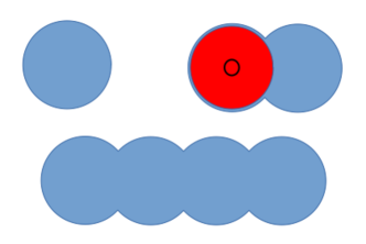
Figure 1: Chains of one, two and four overlapping cavities. The chain of length two shows a hard disk and the small black circle is the volume accessible to its center in the first cavity.

III.3.1 One particle in a chain of $M$ cavities

To see what happens in the canonical ensemble, consider the case of a chain of  $M$ such cavities in $D$ dimensions. The case of $N_{c}=1$ is referred to as a ”zero-dimensional” system in the limit that the cavity is just large enough to hold a single particle. Elementary evaluations lead to

$$Z_{1}\left[\phi\right] =\sum_{i=1}^{M}e_{i}$$ (42)

$$\rho_{\mathbf{r}} =\frac{e^{-\beta\phi_{\mathbf{r}}}}{Z_{1}\left[\phi\right]}\sum_{i=1}^{M}\delta\left(\mathbf{r}\in V_{1}\right)$$

so that

$$e^{-\beta\phi_{\mathbf{r}}}=Z_{1}\left[\phi\right]\Lambda_{T}^{D}\rho_{\mathbf{r}}$$ (43)

and

$$\beta F_{1}\left[\rho\right] =-\ln\left(Z_{1}\left[\phi\left[\rho\right]\right]\right)+\int\rho_{\mathbf{r}}\ln\left(Z_{1}\left[\phi\left[\rho\right]\right]\Lambda_{T}^{D}\rho_{\mathbf{r}}\right)d\mathbf{r}$$ (44)

$$=\int\rho_{\mathbf{r}}\ln\left(\Lambda_{T}^{D}\rho_{\mathbf{r}}\right)d\mathbf{r}$$

which is the ideal-gas result, as one would guess. For comparison, the grand-canonical functional is

$$\beta F\left[\rho\right]=\beta F^{\left(\text{id}\right)}\left[\rho\right]+\Phi\left(\sum_{i=1}^{M}N_{1}\right)$$ (45)

with $\Phi\left(x\right)=\left(1-x\right)\ln\left(1-x\right)+x$ (see, e.g. Ref.Lutsko (2020)). The excess functional - the correction to the ideal gas - is nonzero solely due to the fluctuations in particle number.

III.3.2 Two particles in a chain of three cavities

If the three cavities do not overlap the functional can be guessed based on the preceding results. In the new case of a chain of overlapping cavities the results in both ensembles are non-trivial. We first consider the grand canonical ensemble for which the partition function is

$$\Xi_{\mu}\left[\phi\right]=1+e_{1}+e_{2}+e_{3}+e_{1}e_{3}$$ (46)

giving the density

$$\rho_{\mu\mathbf{r}}=e^{-\beta\left(\phi_{\mathbf{r}}-\mu\right)}\frac{\left(1+e_{3}\right)\delta\left(\mathbf{r}\in V_{1}\right)+\delta\left(\mathbf{r}\in V_{2}\right)+\left(1+e_{1}\right)\delta\left(\mathbf{r}\in V_{3}\right)}{\Xi_{\mu}\left[\phi\right]}$$ (47)

This is integrated over each cavity to get

$$N_{1}=\frac{1+e_{3}}{\Xi_{\mu}\left[\phi\right]}e_{1},\;N_{2}=\frac{1}{\Xi_{\mu}\left[\phi\right]}e_{2},\;N_{3}=\frac{1+e_{1}}{\Xi_{\mu}\left[\phi\right]}e_{3}$$ (48)

and from this system we find

$$e_{1} =\frac{N_{1}}{1-N_{1}-N_{2}},e_{2}=\frac{N_{2}-N_{2}^{2}}{\left(N_{2}+N_{3}-1\right)\left(N_{1}+N_{2}-1\right)},e_{3}=\frac{N_{3}}{1-N_{2}-N_{3}}$$ (49)

$$\Xi =\frac{1-N_{2}}{\left(N_{1}+N_{2}-1\right)\left(N_{2}+N_{3}-1\right)}$$

and

$$e^{-\beta\left(\phi_{\mathbf{r}}-\mu\right)}=\Xi_{\mu}\left[\phi\right]\rho_{\mu\mathbf{r}}\left\{\left(1-\frac{N_{3}}{1-N_{2}}\right)\delta\left(\mathbf{r}\in V_{1}\right)+\delta\left(\mathbf{r}\in V_{2}\right)+\left(1-\frac{N_{1}}{1-N_{2}}\right)\delta\left(\mathbf{r}\in V_{3}\right)\right\}$$ (50)

so that the grand canonical functional is

$$\beta F\left[\rho\right]=\int\rho_{\mathbf{r}}\ln\rho_{\mathbf{r}}d\mathbf{r}-N_{1}\ln\left(\frac{N_{3}}{1-N_{2}}\right)-N_{3}\ln\left(\frac{N_{1}}{1-N_{2}}\right)$$ (51)

In the canonical ensemble, one particle is an ideal gas so we turn to the case of two particles. Here

$$Z_{2}\left[\phi\right] =e_{1}e_{3}$$ (52)

$$\rho_{2\mathbf{r}} =\frac{e^{-\beta\phi_{\mathbf{r}}}}{e_{1}}\delta\left(\mathbf{r}\in V_{1}\right)+\frac{e^{-\beta\phi_{\mathbf{r}}}}{e_{3}}\delta\left(\mathbf{r}\in V_{3}\right)$$

so

$$e^{-\beta\phi_{\mathbf{r}}}=e_{1}\rho_{2\mathbf{r}}\delta\left(\mathbf{r}\in V_{1}\right)+e_{3}\rho_{2\mathbf{r}}\delta\left(\mathbf{r}\in V_{3}\right)$$ (53)

and it follows that

$$\beta F_{2}\left[\rho\right]=\int_{V_{1}}\rho_{\mathbf{r}}\ln\rho_{\mathbf{r}}d\mathbf{r+}\int_{V_{3}}\rho_{\mathbf{r}}\ln\rho_{\mathbf{r}}d\mathbf{r}$$ (54)

which is not an ideal gas unless the potential happens to forbid occupancy (i.e. to be infinite) in the middle cavity. Note that there are several a priori constraints on the density: $N_{1}=N_{3}=1$ and $N_{2}=0$.

III.3.3 Two particles in a chain of four cavities

For two particles in a chain of four cavities, the canonical partition function is

$$Z_{2}\left[\phi\right]=e_{1}e_{3}+e_{1}e_{4}+e_{2}e_{4}$$ (55)

and repeating the usual steps one finds the field

$$Z_{2}\left[\phi\right]e^{-\beta\phi_{\mathbf{r}}}=\frac{1}{e_{3}+e_{4}}\rho_{2\mathbf{r}}\delta\left(\mathbf{r}\in V_{1}\right)+\frac{1}{e_{4}}\rho_{2\mathbf{r}}\delta\left(\mathbf{r}\in V_{2}\right)+\frac{1}{e_{3}}\rho_{2\mathbf{r}}\delta\left(\mathbf{r}\in V_{3}\right)+\frac{1}{e_{1}+e_{2}}\rho_{2\mathbf{r}}\delta\left(\mathbf{r}\in V_{4}\right)$$ (56)

giving the Helmholtz functional

$$F_{2}\left[\rho\right] =\int\rho_{2\mathbf{r}}\ln\rho_{2\mathbf{r}}d\mathbf{r}+N_{1}\ln\frac{1}{e_{3}+e_{4}}+N_{2}\ln\frac{1}{e_{4}}+N_{3}\ln\frac{1}{e_{1}}+N_{4}\ln\frac{1}{e_{1}+e_{2}}$$ (57)

$$+\ln\left(e_{1}e_{3}+e_{1}e_{4}+e_{2}e_{4}\right)$$

with the constants determined from

$$Z_{2}\left[\phi\right]N_{1} =\left(e_{3}+e_{4}\right)e_{1}$$ (58)

$$Z_{2}\left[\phi\right]N_{2} =e_{2}e_{4}$$

$$Z_{2}\left[\phi\right]N_{3} =e_{1}e_{3}$$

$$Z_{2}\left[\phi\right]N_{4} =\left(e_{1}+e_{2}\right)e_{4}$$

The physical requirements that one particle be in one of the first two cavities and the second in one of the last are reflected in the degeneracy $N_{1}+N_{2}=N_{3}+N_{4}=1$, so there are only two independent equations giving, e.g.

$$\frac{N_{1}}{N_{3}} =\frac{e_{4}}{e_{3}}+1\rightarrow e_{3}=e_{4}\left(\frac{N_{1}}{N_{3}}-1\right)^{-1}$$ (59)

$$\frac{N_{4}}{N_{2}} =\frac{e_{1}}{e_{2}}+1\rightarrow e_{2}=e_{1}\left(\frac{N_{4}}{N_{2}}-1\right)^{-1}$$

and finally

$$F_{2}\left[\rho\right] =\int\rho_{2\mathbf{r}}\ln\rho_{2\mathbf{r}}d\mathbf{r}+N_{1}\ln\left(1-\frac{N_{3}}{N_{1}}\right)+N_{4}\ln\left(1-\frac{N_{2}}{N_{4}}\right)-\ln\left(\frac{N_{1}N_{4}-N_{2}N_{3}}{\left(N_{1}-N_{3}\right)\left(N_{4}-N_{2}\right)}\right)$$ (60)

$$=\int\rho_{2\mathbf{r}}\ln\rho_{2\mathbf{r}}d\mathbf{r}+\left(N_{1}+N_{4}+1\right)\ln\left(N_{1}-N_{3}\right)-N_{1}\ln N_{1}-N_{4}\ln N_{4}$$

For comparison, the grand canonical ensemble gives

$$\Xi\left[\phi\right]=1+e_{1}+e_{2}+e_{3}+e_{4}+e_{1}e_{3}+e_{1}e_{4}+e_{2}e_{4}$$ (61)

and

$$e_{1} =\frac{N_{1}}{1-N_{1}-N_{2}}$$ (62)

$$e_{2} =\frac{N_{2}\left(N_{2}-1\right)}{\left(1-N_{2}-N_{3}\right)\left(N_{1}+N_{2}-1\right)}$$

$$e_{3} =\frac{N_{3}\left(N_{3}-1\right)}{\left(1-N_{2}-N_{3}\right)\left(N_{3}+N_{4}-1\right)}$$

$$e_{4} =\frac{N_{4}}{1-N_{3}-N_{4}}$$

yielding

$$\beta F\left[\rho\right] \equiv\int\rho_{\mathbf{r}}\ln\left(\rho_{\mathbf{r}}\right)d\mathbf{r}+\left(1-N_{1}-N_{3}-N_{4}\right)\ln\left(1-N_{2}\allowbreak\right)$$ (63)

$$+\left(1\allowbreak-N_{1}-N_{2}-N_{4}\right)\ln\left(1-N_{3}\allowbreak\right)$$

$$-\left(1-N_{1}-N_{4}\right)\ln\left(1-N_{2}-N_{3}\right)$$

$$-\left(1-N_{3}-N_{4}\right)\ln\left(1-N_{1}-N_{2}\allowbreak\right)$$

$$-\left(1-N_{1}-N_{2}\right)\ln\left(1-N_{3}-N_{4}\right)$$

III.3.4 Comments on v-representability

Notice that all of these results imply certain limits on v-representability. For example, in the case of a single cavity, in the grand-canonical ensemble the average particle number is restricted to be $N_{1}<1$ (see Eq. 45). In the case of a chain of four cavities, in the canonical ensemble one has that $N_{1}+N_{2}=N_{3}+N_{4}=1$ since there must be two particles and since adjacent cavities cannot be simultaneously occupied. Any density violating these constraints cannot be generated by a field. Similarly, in the grand-canonical ensemble, it must be that $N_{1}+N_{2}<1$ and $N_{3}+N_{4}<1$ for similar reasons: when there are zero particles, both sums are zero, when there is one particle neither sum can be greater than one and for two particles the canonical condition holds. So, the weighted average of these giving the grand-canonical result is necessarily less than one and any density violating this is not v-representable.

IV Hard rods in a cavity

Two classes of exactly solvable models have played important roles in the development of modern cDFT in the grand-canonical ensemble. The first is that of hard-spheres in one dimension, also known as hard rods. The exact Helmholtz functional for hard rods was found by Percus in 1976 and will be given below. As of now, no equivalent result is known for the canonical ensemble. Attempts to generalize Percus’ result to higher dimensions eventually led to the development of Fundamental Measure Theory (FMT) which is widely viewed as the most sophisticated model functional. The development of FMT was further guided by the second class of exact models, already discussed above, which are hard particles in small cavities.

IV.1 Grand-canonical

In the grand-canonical ensemble, the exact Helmholtz functional for the case of a single species of hard-rods of length $\sigma$ can be written as

$$F\left[\rho\right]=\int_{-\infty}^{\infty}\rho_{x}\left(\ln\rho_{x}-1\right)dx-\int_{-\infty}^{\infty}s_{x}\left[\rho\right]\ln\left(1-\eta_{x}\left[\rho\right]\right)dx$$ (64)

with

$$\eta_{x}\left[\rho\right] =1-\int_{x-\frac{\sigma}{2}}^{x+\frac{\sigma}{2}}\rho_{y}dy$$ (65)

$$s_{x}\left[\rho\right] =\frac{1}{2}\left(\rho_{x-\frac{\sigma}{2}}+\rho_{x+\frac{\sigma}{2}}\right).$$

If there is a hard wall at $x=0$ and at $x=L$ that means that the center of a hard rod is confined to the domain $\left[\frac{\sigma}{2},L-\frac{\sigma}{2}\right]$ and so the external field is infinite and the density $\rho_{x}=0$ outside this domain. Consider the case that $L<2\sigma$ so that the cavity can only hold a single rod. Some elements of the grand canonical ensemble will have zero rods and some will have one rod so the average total particle number is between zero and one. In general, $\eta_{x}\left[\rho\right]$ will therefore always be between zero and one. Furthermore, if $x-\frac{\sigma}{2}<\frac{\sigma}{2}$, so that $\rho_{x-\frac{\sigma}{2}}=0$ then $x<\sigma$ and so $x+\frac{\sigma}{2}<\frac{3\sigma}{2}<L-\frac{\sigma}{2}$ so $s_{x}\left[\rho\right]$gives (in general) a nonzero contribution. This is all to say that the non-ideal gas part of $F\left[\rho\right]$ contributes, as expected. Nothing conceptually changes as the size of the cavity increases except that the maximum value of the average number of particles.

IV.2 Canonical Ensemble

As noted above, a single particle in a cavity is just an ideal gas, so the simplest nontrivial example would involve two particles. In the following, it is assumed that the length of the cavity is in the range $3\sigma<L<4\sigma$. The reason for not directly considering the possibility $2\sigma<L<3\sigma$ is that it gives rise to mathematical difficulties that will be discussed below.

IV.2.1 The local density

The partition function for the system is

$$Z_{2}\left[\phi\right]=\frac{1}{2!}\Lambda_{T}^{2}\int_{\frac{\sigma}{2}}^{\frac{5\sigma}{2}+\Delta}\int_{\frac{\sigma}{2}}^{\frac{5\sigma}{2}+\Delta}e^{-\beta\phi_{y_{1}}}e^{-\beta\phi_{y_{2}}}\Theta\left(\left|y_{1}-y_{2}\right|-\sigma\right)dy_{1}dy_{2}$$ (66)

where $L=3\sigma+\Delta$ and so $0<\Delta<\sigma$ and the step function $\Theta\left(z\right)=1$ for $z>0$ and zero otherwise. The local density is

$$Z_{2}\left[\phi\right]\Lambda_{T}^{2}\rho_{x}=\Theta\left(\frac{5\sigma}{2}+\Delta-x\right)\Theta\left(x-\frac{\sigma}{2}\right)e^{-\beta\phi_{x}}\int_{\frac{\sigma}{2}}^{\frac{5\sigma}{2}+\Delta}e^{-\beta\phi_{y}}\Theta\left(\left|x-y\right|-\sigma\right)dy$$ (67)

which can be written more explicitly as

$$Z_{2}\left[\phi\right]\Lambda_{T}^{2}\rho_{x} =\Theta\left(\frac{5\sigma}{2}+\Delta-x\right)\Theta\left(x-\frac{3\sigma}{2}\right)e^{-\beta\phi_{x}}\int_{\frac{\sigma}{2}}^{x-\sigma}e^{-\beta\phi_{y}}dy$$ (68)

$$+\Theta\left(\frac{3\sigma}{2}+\Delta-x\right)\Theta\left(x-\frac{\sigma}{2}\right)e^{-\beta\phi_{x}}\int_{x+\sigma}^{\frac{5\sigma}{2}+\Delta}e^{-\beta\phi_{y}}dy$$

or, even more explicitly, the density is zero except for

$$\Lambda_{T}^{2}Z^{\left(2\right)}\left[\phi\right]\rho_{x} =e^{-\beta\phi_{x}}\int_{x+\sigma}^{\frac{5\sigma}{2}+\Delta}e^{-\beta\phi_{y}}dy,\;\;\;\;\;\;\;\;\;\;\;\;\;\;\;\;\;\;\;\;\;\;\frac{\sigma}{2}<x<\frac{3\sigma}{2}$$ (69a)

$$=e^{-\beta\phi_{x}}\int_{\frac{\sigma}{2}}^{x-\sigma}e^{-\beta\phi_{y}}dy+e^{-\beta\phi_{x}}\int_{x+\sigma}^{\frac{5\sigma}{2}+\Delta}e^{-\beta\phi_{y}}dy,\;\frac{3\sigma}{2}<x<\frac{3\sigma}{2}+\Delta$$ (69b)

$$=e^{-\beta\phi_{x}}\int_{\frac{\sigma}{2}}^{x-\sigma}e^{-\beta\phi_{y}}dy,\;\;\;\;\;\;\;\;\;\;\;\;\;\;\;\;\;\;\;\;\;\;\;\;\frac{3\sigma}{2}+\Delta<x<\frac{5\sigma}{2}+\Delta.$$ (69c)

One sees immediately that the function $$\rho_{x}e^{\beta\phi_{x}}$$ is continuous although its first derivative is not and in fact satisfies the jump conditions

$$\lim_{\epsilon\rightarrow 0}\left(\frac{d}{dx}\rho_{x}e^{\beta\phi_{x}}\right)_{\frac{3\sigma}{2}+\epsilon} =\lim_{\epsilon\rightarrow 0}\left(\frac{d}{dx}\rho_{x}e^{\beta\phi_{x}}\right)_{\frac{3\sigma}{2}-\epsilon}+\frac{1}{\Lambda_{T}^{2}Z^{\left(2\right)}\left[\phi\right]}e^{-\beta\phi_{\frac{\sigma}{2}}}$$ (70)

$$\lim_{\epsilon\rightarrow 0}\left(\frac{d}{dx}\rho_{x}e^{\beta\phi_{x}}\right)_{\frac{3\sigma}{2}+\Delta+\epsilon} =\lim_{\epsilon\rightarrow 0}\left(\frac{d}{dx}\rho_{x}e^{\beta\phi_{x}}\right)_{\frac{3\sigma}{2}+\Delta-\epsilon}+\frac{1}{\Lambda_{T}^{2}Z^{\left(2\right)}\left[\phi\right]}e^{-\beta\phi_{\frac{5\sigma}{2}+\Delta}}$$

The density also obeys the relation

$$\rho_{x}e^{\beta\phi_{x}}+\rho_{x+2\sigma}e^{\beta\phi_{x+2\sigma}}=\frac{1}{\Lambda_{T}^{2}Z^{\left(2\right)}\left[\phi\right]}\int_{\frac{\sigma}{2}}^{\frac{5\sigma}{2}+\Delta}e^{-\beta\phi_{y}}dy\equiv A,\;\;\;\;\;\frac{\sigma}{2}<x<\frac{\sigma}{2}+\Delta$$ (71)

which is easily verified by substituting the appropriate expressions for the density from Eq.(85). This will be referred to as the ”duality” relation since it tells us that the functions $\rho_{x}e^{\beta\phi_{x}}$ in the domains $\frac{\sigma}{2}<x<\frac{\sigma}{2}+\Delta$ and $\frac{5\sigma}{2}<x<\frac{5\sigma}{2}+\Delta$ are trivially related.

IV.2.2 Differential relations

Multiplying Eq.(85) by $e^{\beta\phi_{x}}$ and taking the derivative gives a new set of relations

$$\Lambda^{2}Z^{\left(2\right)}\left[\phi\right]\frac{d}{dx}\left(e^{\beta\phi_{x}}\rho_{x}\right) =-e^{-\beta\phi_{x+\sigma}},\;\;\;\;\;\;\;\;\;\;\frac{\sigma}{2}<x<\frac{3\sigma}{2}$$ (72a)

$$\Lambda^{2}Z^{\left(2\right)}\left[\phi\right]\frac{d}{dx}\left(e^{\beta\phi_{x}}\rho_{x}\right) =e^{-\beta\phi_{x-\sigma}}-e^{-\beta\phi_{x+\sigma}},\;\frac{3\sigma}{2}<x<\frac{3\sigma}{2}+\Delta$$

$$\Lambda^{2}Z^{\left(2\right)}\left[\phi\right]\frac{d}{dx}\left(e^{\beta\phi_{x}}\rho_{x}\right) =e^{-\beta\phi_{x-\sigma}},\;\;\;\;\;\;\;\;\;\;\;\frac{3\sigma}{2}+\Delta<x<\frac{5\sigma}{2}+\Delta$$

and shifting the spatial variable in the first and third of these gives

$$\Lambda^{2}Z^{\left(2\right)}\left[\phi\right]\frac{d}{dx}\left(e^{\beta\phi_{x-\sigma}}\rho_{x-\sigma}\right) =-e^{-\beta\phi_{x}},\;\;\;\;\;\;\;\;\;\;\frac{3\sigma}{2}<x<\frac{5\sigma}{2}$$ (73a)

$$\Lambda^{2}Z^{\left(2\right)}\left[\phi\right]\frac{d}{dx}\left(e^{\beta\phi_{x}}\rho_{x}\right) =e^{-\beta\phi_{x-\sigma}}-e^{-\beta\phi_{x+\sigma}},\;\frac{3\sigma}{2}<x<\frac{3\sigma}{2}+\Delta$$ (73b)

$$\Lambda^{2}Z^{\left(2\right)}\left[\phi\right]\frac{d}{dx}\left(e^{\beta\phi_{x+\sigma}}\rho_{x+\sigma}\right) =e^{-\beta\phi_{x}},\;\;\;\;\;\;\;\;\;\;\;\;\;\frac{\sigma}{2}+\Delta<x<\frac{3\sigma}{2}+\Delta.$$ (73c)

Taking advantage of overlaps between the regions in Eq.(85) and Eq.(88) and repeatedly using the duality relation and shifts of the spatial arguments (see Supplementary TextSI ) results in a closed systems of equations which can be partially solved with the result:

$$\frac{d}{dx}\frac{\rho_{x+\sigma}}{\frac{d}{dx}\left(e^{\beta\phi_{x}}\rho_{x}\right)} =\frac{\rho_{x+2\sigma}}{A-\rho_{x}e^{\beta\phi_{x}}}-e^{-\beta\phi_{x}},\;\;\;\;\;\;\;\;\;\;\;\;\;\;\;\;\;\;\;\;\frac{\sigma}{2}<x<\frac{\sigma}{2}+\Delta\equiv D_{1}$$ (74a)

$$e^{-\beta\phi_{x}} =e^{-\beta\phi_{\frac{\sigma}{2}+\Delta}}\frac{\rho_{x}}{\rho_{{}_{\frac{\sigma}{2}+\Delta}}}\exp\left(\int_{\frac{\sigma}{2}+\Delta}^{x}\frac{\rho_{y+\sigma}}{\lambda_{y}\left[\rho\right]}dy\right),\;\;\frac{\sigma}{2}+\Delta<x<\frac{3\sigma}{2}\equiv D_{2}$$ (74b)

$$e^{-\beta\phi_{x}} =\pm\Lambda^{2}Z^{\left(2\right)}\left[\phi\right]\frac{d}{dx}\left(e^{\beta\phi_{x\pm\sigma}}\rho_{x\pm\sigma}\right),\;\;\;\;\;\;\;\;\;\;\;\frac{3\sigma}{2}<x<\frac{3\sigma}{2}+\Delta\equiv D_{3}$$ (74c)

$$e^{-\beta\phi_{x}} =e^{-\beta\phi_{\frac{5\sigma}{2}}}\frac{\rho_{x}}{\rho_{\frac{5\sigma}{2}}}\exp\left(\int_{x-\sigma}^{\frac{3\sigma}{2}}\frac{\rho_{y}}{\lambda_{y}\left[\rho\right]}dy\right),\;\;\;\;\frac{3\sigma}{2}+\Delta<x<\frac{5\sigma}{2}\equiv D_{4}$$ (74d)

$$e^{-\beta\phi_{x}} =\frac{\rho_{x}}{A-e^{\beta\phi_{x-2\sigma}}\rho_{x-2\sigma}},\;\;\;\;\;\;\;\;\;\;\;\;\;\;\;\;\;\;\;\;\;\;\frac{5\sigma}{2}<x<\frac{5\sigma}{2}+\Delta\equiv D_{5}$$ (74e)

with

$$\lambda_{x}\left[\rho\right] =\lambda_{\frac{\sigma}{2}+\Delta}+\int_{\frac{\sigma}{2}+\Delta}^{\frac{3\sigma}{2}+\Delta}\rho_{y}dy-\int_{x}^{x+\sigma}\rho_{y}dy=\lambda_{\frac{\sigma}{2}+\Delta}+\int_{\frac{\sigma}{2}+\Delta}^{x}\rho_{y}dy-\int_{\frac{3\sigma}{2}+\Delta}^{x+\sigma}\rho_{y}dy$$ (75)

$$\Lambda^{2}Z^{\left(2\right)}\left[\phi\right] =\frac{1}{e^{\beta\phi_{\frac{5\sigma}{2}}}\rho_{\frac{5\sigma}{2}}}\frac{1}{e^{\beta\phi_{\frac{\sigma}{2}+\Delta}}\rho_{{}_{\frac{\sigma}{2}+\Delta}}}\lambda_{\frac{\sigma}{2}+\Delta}\left[\rho\right]\exp\left(\int_{\frac{\sigma}{2}+\Delta}^{\frac{3\sigma}{2}}\frac{\rho_{y}}{\lambda_{y}\left[\rho\right]}dy\right)$$

Names have been assigned to various domains and the physical significance of these divisions is as follows: the domain $D_{3}$ is the only one which both hard rods can visit. When the rightmost rod is in this range, the leftmost is confined to $D_{1}$ and when the leftmost is in the overlap range, the rightmost is confined to $D_{5}$. The leftmost rod can be in the range $D_{2}$ when the when the rightmost rod is not in the overlap region, $D_{3}$, and vice versa for $D_{4}$. In the course of solving the equations, the following constraints are generated:

$$\int_{\frac{\sigma}{2}}^{\frac{\sigma}{2}+\Delta}e^{-\beta\phi_{y}}dy =e^{-\beta\phi_{\frac{\sigma}{2}+\Delta}}\frac{1}{\rho_{{}_{\frac{\sigma}{2}+\Delta}}}\lambda_{\frac{\sigma}{2}+\Delta}$$ (76a)

$$\int_{\frac{5\sigma}{2}}^{\frac{5\sigma}{2}+\Delta}e^{-\beta\phi_{y}}dy =e^{-\beta\phi_{\frac{5\sigma}{2}}}\frac{1}{\rho_{\frac{5\sigma}{2}}}\lambda_{\frac{3\sigma}{2}}$$

$$-\frac{\rho_{\frac{\sigma}{2}+\Delta}e^{\beta\phi_{\frac{\sigma}{2}+\Delta}}}{\left(\rho_{x}e^{\beta\phi_{x}}\right)_{\frac{\sigma}{2}+\Delta}^{\prime}}\rho_{\frac{3\sigma}{2}+\Delta}+\int_{\frac{\sigma}{2}+\Delta}^{\frac{3\sigma}{2}}\rho_{y}dy =\frac{\rho_{\frac{5\sigma}{2}}e^{\beta\phi_{\frac{5\sigma}{2}}}}{\left(\rho_{x}e^{\beta\phi_{x}}\right)_{\frac{5\sigma}{2}}^{\prime}}\rho_{\frac{3\sigma}{2}}+\int_{\frac{3\sigma}{2}+\Delta}^{\frac{5\sigma}{2}}\rho_{z}dz.$$

The solution of Eq.(74) involves 6 integration constants: two from the ode in domain  $$D_{1} e^{-\beta\phi_{\frac{\sigma}{2}+\Delta}},e^{-\beta\phi_{\frac{5\sigma}{2}}},\lambda_{\frac{\sigma}{2}+\Delta} A \rho_{x}e^{\beta\phi_{x}} A A A$$, and . Continuity of the quantity across the boundaries of the domains gives four conditions and the first two of Eq.(76a) already give six. There is also the definition of , Eq(87), the jump conditions, Eq.(86), and the last of Eq.(76a): clearly, many of these are redundant. In fact, based on the solution given here, one can easily show that the jump conditions are automatically satisfied and that the evaluation of from its definition ends in a tautology giving no new information. Also, the second of the relations in Eq.(76a) follows from the first as is easily shown using Eq.(88b) and the third relation also follows from the definitions. So, in the end, there are only the four continuity relations and the first of Eq.(76a) and the indeterminacy of the parameter represents the gauge freedom of the potential.

As a simple illustration of these results, note first that in the case of no field (or, more generally, a constant field), the density is a piece-wise-linear function

$$\Lambda_{T}^{2}Z^{\left(2\right)}\left[\phi\right]\rho_{x} =\left(\Delta-x+\frac{3}{2}\sigma\right),\;\;\;\;\;\;\;\;\;\;\;\;\;\;\;\;\;\;\;\;\;\;\frac{\sigma}{2}<x<\frac{3\sigma}{2}$$ (77a)

$$=\Delta,\;\frac{3\sigma}{2}<x<\frac{3\sigma}{2}+\Delta$$

$$=\left(x-\frac{3}{2}\sigma\right),\;\;\;\;\;\;\;\;\;\;\;\;\;\;\;\;\;\;\;\;\;\;\;\;\frac{3\sigma}{2}+\Delta<x<\frac{5\sigma}{2}+\Delta.$$

with

$$\Lambda_{T}^{2}Z^{\left(2\right)}\left[\phi\right]=\frac{1}{2}\left(\Delta+\sigma\right)^{2}$$ (78)

The field as a function of the density can be solved analytically for the case of a constant density $\rho_{x}=\frac{2}{2\sigma+\Delta}$ throughout $\frac{\sigma}{2}<x<\frac{5\sigma}{2}+\Delta$ with the result

$$e^{-\beta\phi_{x}} =\frac{\rho}{A}\left(1+e^{B\left(x-\frac{1}{2}\sigma-\frac{\Delta}{2}\right)}\right),\;\;\;\;\;\;\;\;\;\;\;\;\;\;\;\;\;\;\;\;\;\;\;\;\frac{\sigma}{2}<x<\frac{\sigma}{2}+\Delta$$ (79a)

$$=\frac{\rho}{A}\frac{B\Delta}{B\Delta-2}e^{-\frac{2}{\Delta}\left(\frac{\sigma}{2}+\Delta-x\right)},\;\;\;\;\;\;\;\;\;\;\;\;\;\;\;\;\;\;\;\;\;\;\;\frac{\sigma}{2}+\Delta<x<\frac{3\sigma}{2}$$

$$=\frac{\rho}{A}\frac{\left(B\Delta\right)^{3}}{4\left(B\Delta-2\right)}e^{-\frac{2}{\Delta}\left(\Delta-\sigma\right)}\frac{e^{B\left(x-\frac{3}{2}\sigma\right)}}{\left(1+e^{B\left(x-\frac{3}{2}\sigma-\frac{\Delta}{2}\right)}\right)^{2}},\;\frac{3\sigma}{2}<x<\frac{3\sigma}{2}+\Delta$$

$$=\frac{\rho}{A}\frac{B\Delta}{B\Delta-2}e^{-\frac{2}{\Delta}\left(x-\frac{5}{2}\sigma\right)},\;\;\;\;\;\;\;\;\;\;\;\;\;\;\;\;\;\;\;\;\;\;\;\;\frac{3\sigma}{2}+\Delta<x<\frac{5\sigma}{2}$$

$$=\frac{\rho}{A}\left(1+e^{B\left(\frac{5}{2}\sigma+\frac{\Delta}{2}-x\right)}\right),\;\;\;\;\;\;\;\;\;\;\;\;\;\;\;\;\;\;\;\;\;\;\;\;\;\frac{5\sigma}{2}<x<\frac{5\sigma}{2}+\Delta$$

where, $$A \phi_{x}-k_{B}T\ln A B B\Delta=2+2W\left(e^{-1}\right)\approx 2.\,\allowbreak 556\,92 W(x)$$ is the expected arbitrary constant (so that the family of equivalent potentials is ), the constant is determined from where is the Lambert W-function and the partition function is

$$\Lambda^{2}Z^{\left(2\right)}\left[\phi\right]=\left(\frac{B\Delta}{A\left(B\Delta-2\right)}\right)^{2}\frac{1}{2}\rho\Delta e^{-\frac{2}{\Delta}\left(\Delta-\sigma\right)}.$$ (80)

IV.2.3 The Helmholtz functional

The Helmholtz functional is determined from Eq.(25) as in the case of the ideal gas (see Supplementary TextSI ). Not all contributions can be explicitly worked out but a useful result is still possible in the form

$$F\left[\rho\right]=\int_{\frac{\sigma}{2}}^{\frac{5\sigma}{2}}\rho_{x}\left(\ln\Lambda_{T}\rho_{x}-1\right)dx-\int_{\sigma}^{2\sigma}s_{x}\left[\rho\right]\ln\left(1-\eta_{x}\left[\rho\right]\right)dx+O\left(\frac{\Delta}{\sigma}\right).$$ (81)

In fact the limit $\frac{\Delta}{\sigma}=0$ can be derived directly but there are certain ambiguities which, in this extended calculation, resolve as terms which separately diverge in the limit $\frac{\Delta}{\sigma}\rightarrow 0$ but which are collectively finite for all $\frac{\Delta}{\sigma}$. This was, in fact, the reason for considering this more general system. It is interesting to note that the origin of the singularities lies in the physical fact that for a cavity of length $3\sigma$, the center of one rod is confined to $\left[\frac{\sigma}{2},\frac{3\sigma}{2}\right]$ and that of the second to $\left[\frac{3\sigma}{2},\frac{5\sigma}{2}\right]$ so that $\rho_{\frac{3\sigma}{2}}=0$ and $\eta_{\sigma}\left[\rho\right]=\eta_{2\sigma}\left[\rho\right]=1$ , the latter fact leading to difficulties with the log in Eq.(81).

V Conclusions

It has been shown that the mapping between the external field and the density in both the canonical and grand-canonical ensembles is virtually identical with the only difference being an unimportant freedom in the canonical ensemble to shift the field arbitrarily (and this freedom can be removed by imposing a gauge condition). As a consequence, DFT in the two ensembles is formally identical and this is explicitly seen in the case of the ideal gas for which the functionals are almost the same in the two ensembles. Beyond the ideal gas, there are only a few systems for which exact results have been derived in the grand-canonical ensemble: hard particles in small cavities that can only hold a single particle and, at the other extreme, hard rods in one dimension with no constraint on the geometry (and slight generalizations, such as sticky hard rods). It was shown here that for chains of small cavities, results for small cavities can be easily obtained in the canonical ensemble. These can do doubt be extended, as in the grand-canonical ensemble, to other interesting topologiesLutsko (2020). Finally, the important case of hard-rods in one dimension was considered where the general exact result for the grand-canonical ensemble is known. In this case, the canonical ensemble seems to be more difficult to work with and in fact, the problem of even two hard rods in a restricted geometry turns out to be difficult to solve explicitly although a formal solution was constructed. A remarkable aspect of the resulting Helmholtz functional was the close similarity it has to the general grand-canonical result. This can be made even more apparent by writing them together:

$$F\left[\rho\right] =\int_{\frac{\sigma}{2}}^{\frac{5\sigma}{2}}\rho_{x}\left(\ln\Lambda_{T}\rho_{x}-1\right)dx-\int_{\sigma}^{2\sigma}s_{x}\left[\rho\right]\ln\left(1-\eta_{x}\left[\rho\right]\right)dx+O\left(\frac{\Delta}{\sigma}\right),\;\text{(C)}$$ (82)

$$F\left[\rho\right] =\int_{\frac{\sigma}{2}}^{\frac{5\sigma}{2}}\rho_{x}\left(\ln\Lambda_{T}\rho_{x}-1\right)dx-\int_{0}^{3\sigma}s_{x}\left[\rho\right]\ln\left(1-\eta_{x}\left[\rho\right]\right)dx,\;\;\;\;\;\;\;\;\;\;\;\;\text{(GC)}$$

so that one sees that to leading order in $\frac{\Delta}{\sigma}$, the only difference is in the limits of the integrals. Nevertheless, the overall complexity of the full result is far more involved than for the grand-canonical ensemble, thus highlighting important differences between them.

Finally, one can only speculate on the broader implications of these results. Clearly, cDFT exists equally rigorously in both the canonical and grand-canonical ensembles. The most important difference between them is in the variety of exact results available on which to base models and even then, the gap is not as large as might be expected. Indeed, in the examples considered here, the functionals show certain similarities of structure. While this might have been anticipated for the ideal gas, it is very surprising that even for a very small system such as the case of two hard-rods, the canonical and grand-canonical Helmholtz functionals can be so similar. While this does not rigorously justify using grand-canonical functionals in canonical models, it does suggest that do so - for lack of better options - is not unreasonable.

The Helmholtz functional

For completeness, the expression for the Helmholtz functional for two rods in a cavity in the canonical ensemble as derived in the Supplementary TextSI is quoted here:

$$\beta F_{2}\left[\rho\right] =F_{2}^{\text{ideal}}\left[\rho_{N}\right]-\int_{\sigma+\Delta}^{2\sigma}s_{x}[\rho]\ln(\Delta\lambda+\eta_{x}[\rho])dx$$ (83)

$$+\left(1-\int_{\frac{\sigma}{2}+\Delta}^{\frac{3\sigma}{2}}\rho_{x}dx\right)\ln\frac{e^{\beta\phi_{\frac{\sigma}{2}+\Delta}}\rho_{{}_{\frac{\sigma}{2}+\Delta}}}{\lambda_{\frac{\sigma}{2}+\Delta}^{1/2}}+\left(1-\int_{\frac{3\sigma}{2}+\Delta}^{\frac{5\sigma}{2}}\rho_{x}dx\right)\ln\frac{e^{\beta\phi_{\frac{5\sigma}{2}}}\rho_{\frac{5\sigma}{2}}}{\lambda_{\frac{3\sigma}{2}}^{1/2}}$$

$$+\frac{1}{2}\left(\int_{\frac{\sigma}{2}+\Delta}^{\frac{3\sigma}{2}}\rho_{y}dy+\lambda_{\frac{\sigma}{2}+\Delta}-1\right)\left(\int_{\frac{\sigma}{2}+\Delta}^{\frac{3\sigma}{2}}\frac{\rho_{y+\sigma}+\rho_{y}}{\lambda_{y}}dy\right)-1$$

$$-\sum_{a=0}^{2}\int_{\frac{\sigma}{2}+a\sigma}^{\frac{\sigma}{2}+a\sigma+\Delta}\rho_{x}\left(\ln e^{\beta\phi_{x}}\rho_{x}-\frac{1}{2}\right)dx$$

where $F_{2}^{\text{ideal}}$ is the ideal gas functional,Eq.(38), $\eta_{x}[\rho],s_{x}[\rho]$ are components of the Percus functional, Eq.(65), and

$$\Delta\lambda\equiv\lambda_{\frac{\sigma}{2}+\Delta}+\int_{\frac{\sigma}{2}+\Delta}^{\frac{3\sigma}{2}+\Delta}\rho_{y}dy-1$$ (84)

Finally, it is important to note that these expressions are not as explicit as they appear since the quantities $\phi_{\frac{\sigma}{2}+\Delta},\phi_{\frac{5\sigma}{2}},\lambda_{\frac{\sigma}{2}+\Delta}$ are all functionals of the density as well as, of course, the explicit contributions in $\phi_{x}[\rho]$.

Supplementary Text

Appendix A Canonical Cavity: the field in terms of the density

The problem concerns two hard rods of length $\sigma$ in a cavity defined by $0\leq x\leq L=3\sigma+\Delta$ with $\Delta<\sigma$ . This means that the centers of a single hard rod is confined to the interval $\frac{\sigma}{2}\leq x\leq\frac{5\sigma}{2}+\Delta$ and so is defined by an external field that is infinite everywhere outside this range. For convenience, we recall the important preliminary results from the main text. The density is

$$\Lambda_{T}^{2}Z^{\left(2\right)}\left[\phi\right]\rho_{x} =e^{-\beta\phi_{x}}\int_{x+\sigma}^{\frac{5\sigma}{2}+\Delta}e^{-\beta\phi_{y}}dy,\;\;\;\;\;\;\;\;\;\;\;\;\;\;\;\;\;\;\;\;\;\;\frac{\sigma}{2}<x<\frac{3\sigma}{2}$$ (85a)

$$=e^{-\beta\phi_{x}}\int_{\frac{\sigma}{2}}^{x-\sigma}e^{-\beta\phi_{y}}dy+e^{-\beta\phi_{x}}\int_{x+\sigma}^{\frac{5\sigma}{2}+\Delta}e^{-\beta\phi_{y}}dy,\;\frac{3\sigma}{2}<x<\frac{3\sigma}{2}+\Delta$$ (85b)

$$=e^{-\beta\phi_{x}}\int_{\frac{\sigma}{2}}^{x-\sigma}e^{-\beta\phi_{y}}dy,\;\;\;\;\;\;\;\;\;\;\;\;\;\;\;\;\;\;\;\;\;\;\;\;\frac{3\sigma}{2}+\Delta<x<\frac{5\sigma}{2}+\Delta.$$ (85c)

and from these one easily demonstrates the jump conditions

$$\lim_{\epsilon\rightarrow 0}\left(\frac{d}{dx}\rho_{x}e^{\beta\phi_{x}}\right)_{\frac{3\sigma}{2}+\epsilon} =\lim_{\epsilon\rightarrow 0}\left(\frac{d}{dx}\rho_{x}e^{\beta\phi_{x}}\right)_{\frac{3\sigma}{2}-\epsilon}+\frac{1}{\Lambda_{T}^{2}Z^{\left(2\right)}\left[\phi\right]}e^{-\beta\phi_{\frac{\sigma}{2}}}$$ (86)

$$\lim_{\epsilon\rightarrow 0}\left(\frac{d}{dx}\rho_{x}e^{\beta\phi_{x}}\right)_{\frac{3\sigma}{2}+\Delta+\epsilon} =\lim_{\epsilon\rightarrow 0}\left(\frac{d}{dx}\rho_{x}e^{\beta\phi_{x}}\right)_{\frac{3\sigma}{2}+\Delta-\epsilon}+\frac{1}{\Lambda_{T}^{2}Z^{\left(2\right)}\left[\phi\right]}e^{-\beta\phi_{\frac{5\sigma}{2}+\Delta}}$$

The duality relation is

$$\rho_{x}e^{\beta\phi_{x}}+\rho_{x+2\sigma}e^{\beta\phi_{x+2\sigma}}=\frac{1}{\Lambda_{T}^{2}Z^{\left(2\right)}\left[\phi\right]}\int_{\frac{\sigma}{2}}^{\frac{5\sigma}{2}+\Delta}e^{-\beta\phi_{y}}dy\equiv A,\;\;\;\;\;\frac{\sigma}{2}<x<\frac{\sigma}{2}+\Delta$$ (87)

and the differential relations derived in the main text are

$$\Lambda^{2}Z^{\left(2\right)}\left[\phi\right]\frac{d}{dx}\left(e^{\beta\phi_{x-\sigma}}\rho_{x-\sigma}\right) =-e^{-\beta\phi_{x}},\;\;\;\;\;\;\;\;\;\;\frac{3\sigma}{2}<x<\frac{5\sigma}{2}$$ (88a)

$$\Lambda^{2}Z^{\left(2\right)}\left[\phi\right]\frac{d}{dx}\left(e^{\beta\phi_{x}}\rho_{x}\right) =e^{-\beta\phi_{x-\sigma}}-e^{-\beta\phi_{x+\sigma}},\;\frac{3\sigma}{2}<x<\frac{3\sigma}{2}+\Delta$$ (88b)

$$\Lambda^{2}Z^{\left(2\right)}\left[\phi\right]\frac{d}{dx}\left(e^{\beta\phi_{x+\sigma}}\rho_{x+\sigma}\right) =e^{-\beta\phi_{x}},\;\;\;\;\;\;\;\;\;\;\;\;\;\frac{\sigma}{2}+\Delta<x<\frac{3\sigma}{2}+\Delta.$$ (88c)

A.1 Solving the canonical cavity

Using Eq.(88a) one can rewrite Eq.(85b) as

$$\rho_{x}=-\frac{d}{dx}\left(e^{\beta\phi_{x-\sigma}}\rho_{x-\sigma}\right)\left\{\int_{\frac{\sigma}{2}}^{x-\sigma}e^{-\beta\phi_{y}}dy+\int_{x+\sigma}^{\frac{5\sigma}{2}+\Delta}e^{-\beta\phi_{y}}dy\right\},\;\frac{3\sigma}{2}<x<\frac{3\sigma}{2}+\Delta$$ (89a)

So

$$\frac{d}{dx}\frac{\rho_{x}}{\frac{d}{dx}\left(e^{\beta\phi_{x-\sigma}}\rho_{x-\sigma}\right)}=-e^{-\beta\phi_{x-\sigma}}+e^{-\beta\phi_{x+\sigma}},\;\frac{3\sigma}{2}<x<\frac{3\sigma}{2}+\Delta$$ (90a)

and shifting gives

$$\frac{d}{dx}\frac{\rho_{x+\sigma}}{\frac{d}{dx}\left(e^{\beta\phi_{x}}\rho_{x}\right)}=-e^{-\beta\phi_{x}}+e^{-\beta\phi_{x+2\sigma}},\;\frac{\sigma}{2}<x<\frac{\sigma}{2}+\Delta$$ (91a)

and the duality relation allows this to be written as

$$\frac{d}{dx}\frac{\rho_{x+\sigma}}{\frac{d}{dx}\left(e^{\beta\phi_{x}}\rho_{x}\right)}=\frac{\rho_{x+2\sigma}}{A-e^{\beta\phi_{x}}\rho_{x}}-e^{-\beta\phi_{x}},\;\frac{\sigma}{2}<x<\frac{\sigma}{2}+\Delta.$$ (92a)

Using it again to replace $$e^{\beta\phi_{x}}\rho_{x} A-\rho_{x+2\sigma}e^{\beta\phi_{x+2\sigma}}$$ by and shifting gives

$$\frac{d}{dx}\frac{\rho_{x-\sigma}}{\frac{d}{dx}\left(e^{\beta\phi_{x}}\rho_{x}\right)}=\frac{\rho_{x-2\sigma}}{A-e^{\beta\phi_{x}}\rho_{x}}-e^{-\beta\phi_{x}},\;\frac{5\sigma}{2}<x<\frac{5\sigma}{2}+\Delta.$$ (93a)

Eq.(88a) then immediately gives

$$e^{-\beta\phi_{x}}=-\Lambda^{2}Z^{\left(2\right)}\left[\phi\right]\frac{d}{dx}\left(e^{\beta\phi_{x-\sigma}}\rho_{x-\sigma}\right)=\Lambda^{2}Z^{\left(2\right)}\left[\phi\right]\frac{d}{dx}\left(e^{\beta\phi_{x+\sigma}}\rho_{x+\sigma}\right),\;\;\;\;\;\;\;\;\;\;\frac{3\sigma}{2}<x<\frac{3\sigma}{2}+\Delta$$ (94)

with the second equality following from duality.

To get the remaining intervals, start with Eq.(85c) and use Eq.(88a) to write

$$\rho_{x}=-\frac{d}{dx}\left(e^{\beta\phi_{x-\sigma}}\rho_{x-\sigma}\right)\int_{\frac{\sigma}{2}}^{x-\sigma}e^{-\beta\phi_{y}}dy,\;\;\frac{3\sigma}{2}+\Delta<x<\frac{5\sigma}{2}.$$ (95a)

Differentiate and shift to get

$$\frac{d}{dx}\frac{\rho_{x+\sigma}}{\frac{d}{dx}\left(e^{\beta\phi_{x}}\rho_{x}\right)}=-e^{-\beta\phi_{x}},\;\;\frac{\sigma}{2}+\Delta<x<\frac{3\sigma}{2}.$$ (96)

The final interval follows from the same process using Eq.(85a) and (88c)

$$\frac{d}{dx}\frac{\rho_{x-\sigma}}{\frac{d}{dx}\left(e^{\beta\phi_{x}}\rho_{x}\right)}=-e^{-\beta\phi_{x}},\;\;\;\;\;\;\;\frac{3\sigma}{2}+\Delta<x<\frac{5\sigma}{2}.$$ (97)

We can then summarize as

$$\frac{d}{dx}\frac{\rho_{x+\sigma}}{\frac{d}{dx}\left(e^{\beta\phi_{x}}\rho_{x}\right)} =\frac{\rho_{x+2\sigma}}{A-\rho_{x}e^{\beta\phi_{x}}}-e^{-\beta\phi_{x}},\;\;\;\;\;\;\;\;\;\frac{\sigma}{2}<x<\frac{\sigma}{2}+\Delta$$ (98)

$$\frac{d}{dx}\frac{\rho_{x+\sigma}}{\frac{d}{dx}\left(e^{\beta\phi_{x}}\rho_{x}\right)} =-e^{\beta\phi_{x}},\;\;\;\;\;\;\;\;\;\;\;\;\;\;\;\;\;\;\;\;\;\;\;\;\;\frac{\sigma}{2}+\Delta<x<\frac{3\sigma}{2}$$

$$e^{-\beta\phi_{x}} =\pm\Lambda^{2}Z^{\left(2\right)}\left[\phi\right]\frac{d}{dx}\left(e^{\beta\phi_{x\pm\sigma}}\rho_{x\pm\sigma}\right),\;\frac{3\sigma}{2}<x<\frac{3\sigma}{2}+\Delta$$

$$\frac{d}{dx}\frac{\rho_{x-\sigma}}{\frac{d}{dx}\left(e^{\beta\phi_{x}}\rho_{x}\right)} =-e^{-\beta\phi_{x}},\;\;\;\;\;\;\;\;\;\;\;\;\;\;\;\;\;\;\;\;\;\;\;\frac{3\sigma}{2}+\Delta<x<\frac{5\sigma}{2}$$

$$\frac{d}{dx}\frac{\rho_{x-\sigma}}{\frac{d}{dx}\left(e^{\beta\phi_{x}}\rho_{x}\right)} =\frac{\rho_{x-2\sigma}}{A-e^{\beta\phi_{x}}\rho_{x}}-e^{-\beta\phi_{x}},\;\;\;\;\;\;\;\;\;\frac{5\sigma}{2}<x<\frac{5\sigma}{2}+\Delta$$

A.2 Explicit solutions

Define

$$w_{x}=\left(e^{\beta\phi_{x}}\rho_{x}\right)^{-1}$$ (99)

and after substituting into the first of Eq.(98) and simplifying one gets

$$\frac{d}{dx}\left(-\frac{w_{x}\rho_{x+\sigma}}{w_{x}^{\prime}}\right)=\rho_{x+\sigma}-\rho_{x},\;\;\frac{\sigma}{2}+\Delta<x<\frac{3\sigma}{2}$$ (100)

so

$$\frac{w_{x}\rho_{x+\sigma}}{w_{x}^{\prime}}=\lambda_{-}\left(x\right)\equiv\left(\frac{w_{x}\rho_{x+\sigma}}{w_{x}^{\prime}}\right)_{\frac{\sigma}{2}+\Delta}-\int_{\frac{\sigma}{2}+\Delta}^{x}\left(\rho_{y+\sigma}-\rho_{y}\right)dy,\;\;\frac{\sigma}{2}+\Delta<x<\frac{3\sigma}{2}.$$ (101)

Solving gives

$$\ln w_{x}=\ln w_{\frac{\sigma}{2}+\Delta}+\int_{\frac{\sigma}{2}+\Delta}^{x}\frac{\rho_{z+\sigma}}{\lambda_{z}^{\left(-\right)}}dz,\;\;\frac{\sigma}{2}+\Delta<x<\frac{3\sigma}{2}$$ (102)

or

$$e^{-\beta\phi_{x}}=e^{-\beta\phi_{\frac{\sigma}{2}+\Delta}}\frac{\rho_{x}}{\rho_{\frac{\sigma}{2}+\Delta}}\exp\left(\int_{\frac{\sigma}{2}+\Delta}^{x}\frac{\rho_{z+\sigma}}{\lambda_{z}^{\left(-\right)}}dz\right),\;\;\frac{\sigma}{2}+\Delta<x<\frac{3\sigma}{2}$$ (103)

so that $e^{-\beta\phi_{\frac{\sigma}{2}+\Delta}}$ and $\lambda_{-}\left(\frac{\sigma}{2}+\Delta\right)$ are the expected two integration constants. Note that since $\frac{d}{dx}\lambda_{-}\left(x\right)=\rho_{x}-\rho_{x+\sigma}$ one has the very useful relations

$$\frac{\rho_{x}}{\rho_{\frac{\sigma}{2}+\Delta}}\exp\left(\int_{\frac{\sigma}{2}+\Delta}^{x}\frac{\rho_{z+\sigma}}{\lambda_{z}^{\left(-\right)}}dz\right)=\frac{\lambda_{\frac{\sigma}{2}+\Delta}^{\left(-\right)}}{\rho_{\frac{\sigma}{2}+\Delta}}\frac{\rho_{x}}{\lambda_{x}^{\left(-\right)}}\exp\left(\int_{\frac{\sigma}{2}+\Delta}^{x}\frac{\rho_{z}}{\lambda_{z}^{\left(-\right)}}dz\right)=\frac{\lambda_{\frac{\sigma}{2}+\Delta}^{\left(-\right)}}{\rho_{\frac{\sigma}{2}+\Delta}}\frac{d}{dx}\exp\left(\int_{\frac{\sigma}{2}+\Delta}^{x}\frac{\rho_{z}}{\lambda_{z}^{\left(-\right)}}dz\right).$$ (104)

Similarly, one finds

$$e^{-\beta\phi_{x}}=e^{-\beta\phi_{\frac{5\sigma}{2}}}\frac{\rho_{x}}{\rho_{\frac{5\sigma}{2}}}\exp\left(-\int_{x}^{\frac{5\sigma}{2}}\frac{\rho_{y-\sigma}}{\lambda_{y}^{\left(+\right)}}dy\right),\;\;\;\;\;\frac{3\sigma}{2}+\Delta<x<\frac{5\sigma}{2}$$ (105)

with

$$\lambda_{x}^{\left(+\right)}=-\frac{\rho_{\frac{5\sigma}{2}}e^{\beta\phi_{\frac{5\sigma}{2}}}}{\left(\rho_{x}e^{\beta\phi_{x}}\right)_{\frac{5\sigma}{2}}^{\prime}}\rho_{\frac{3\sigma}{2}}-\int_{\frac{3\sigma}{2}}^{\frac{5\sigma}{2}}\rho_{z}dz+\int_{x-\sigma}^{x}\rho_{z}dz$$ (106)

and again, since $\frac{d}{dx}\lambda_{x}^{\left(+\right)}=\rho_{x}-\rho_{x-\sigma}$,

$$\frac{\rho_{x}}{\rho_{\frac{5\sigma}{2}}}\exp\left(-\int_{x}^{\frac{5\sigma}{2}}\frac{\rho_{y-\sigma}}{\lambda_{y}^{\left(+\right)}}dy\right)=\frac{\lambda_{\frac{5\sigma}{2}}^{\left(+\right)}}{\rho_{\frac{5\sigma}{2}}}\frac{\rho_{x}}{\lambda_{x}^{\left(+\right)}}\exp\left(-\int_{x}^{\frac{5\sigma}{2}}\frac{\rho_{y}}{\lambda_{y}^{\left(+\right)}}dy\right)=\frac{\lambda_{\frac{5\sigma}{2}}^{\left(+\right)}}{\rho_{\frac{5\sigma}{2}}}\frac{d}{dx}\exp\left(-\int_{x}^{\frac{5\sigma}{2}}\frac{\rho_{y}}{\lambda_{y}^{\left(+\right)}}dy\right).$$ (107)

As a final step, we use both of these together to verify the original relation between density and field, starting with Eq.(85a)

$$\Lambda_{T}^{2}Z^{\left(2\right)}\left[\phi\right]\rho_{x} =e^{-\beta\phi_{x}}\int_{x+\sigma}^{\frac{5\sigma}{2}+\Delta}e^{-\beta\phi_{y}}dy,\;\;\;\;\frac{\sigma}{2}+\Delta<x<\frac{3\sigma}{2}$$ (108)

$$=e^{-\beta\phi_{x}}\left(\int_{\frac{5\sigma}{2}}^{\frac{5\sigma}{2}+\Delta}e^{-\beta\phi_{y}}dy+\int_{x+\sigma}^{\frac{5\sigma}{2}}e^{-\beta\phi_{y}}dy\right)$$

$$=e^{-\beta\phi_{x}}\left(\int_{\frac{5\sigma}{2}}^{\frac{5\sigma}{2}+\Delta}e^{-\beta\phi_{y}}dy+e^{-\beta\phi_{\frac{5\sigma}{2}}}\frac{\lambda_{\frac{5\sigma}{2}}^{\left(+\right)}}{\rho_{\frac{5\sigma}{2}}}-e^{-\beta\phi_{\frac{5\sigma}{2}}}\exp\left(-\int_{x+\sigma}^{\frac{5\sigma}{2}}\frac{\rho_{y}}{\lambda_{y}^{\left(+\right)}}dy\right)\right)$$

where the third line follows from recognizing that the integrand is restricted to the interval $\frac{3\sigma}{2}+\Delta<x<\frac{5\sigma}{2}$ and using the last line of 107. Substituting the solution for the field in $D_{2}$ and simplifying gives

$$\Lambda_{T}^{2}Z^{\left(2\right)}\left[\phi\right] =e^{-\beta\phi_{\frac{\sigma}{2}+\Delta}}\frac{1}{\rho_{\frac{\sigma}{2}+\Delta}}\exp\left(\int_{\frac{\sigma}{2}+\Delta}^{x}\frac{\rho_{z+\sigma}}{\lambda_{z}^{\left(-\right)}}dz\right),\;\;\;\;\frac{\sigma}{2}+\Delta<x<\frac{3\sigma}{2}$$ (109)

$$\times\left(\int_{\frac{5\sigma}{2}}^{\frac{5\sigma}{2}+\Delta}e^{-\beta\phi_{y}}dy+e^{-\beta\phi_{\frac{5\sigma}{2}}}\frac{\lambda_{\frac{5\sigma}{2}}^{\left(+\right)}}{\rho_{\frac{5\sigma}{2}}}-e^{-\beta\phi_{\frac{5\sigma}{2}}}\frac{\lambda_{\frac{5\sigma}{2}}^{\left(+\right)}}{\rho_{\frac{5\sigma}{2}}}\exp\left(-\int_{x+\sigma}^{\frac{5\sigma}{2}}\frac{\rho_{y}}{\lambda_{z}^{\left(+\right)}}dy\right)\right)$$

The left hand side is independent of $x$ so the right hand side must be also. Taking a derivative with respect to $x$ and simplifying gives

$$0=\int_{\frac{5\sigma}{2}}^{\frac{5\sigma}{2}+\Delta}e^{-\beta\phi_{y}}dy+e^{-\beta\phi_{\frac{5\sigma}{2}}}\frac{\lambda_{\frac{5\sigma}{2}}^{\left(+\right)}}{\rho_{\frac{5\sigma}{2}}}-e^{-\beta\phi_{\frac{5\sigma}{2}}}\left(1+\frac{\lambda_{x}^{\left(-\right)}}{\lambda_{x+\sigma}^{\left(+\right)}}\right)\frac{\lambda_{\frac{5\sigma}{2}}^{\left(+\right)}}{\rho_{\frac{5\sigma}{2}}}\exp\left(-\int_{x+\sigma}^{\frac{5\sigma}{2}}\frac{\rho_{y}}{\lambda_{z}^{\left(+\right)}}dy\right)$$ (110)

Another derivative and simplification gives

$$0=\rho_{x}\frac{\lambda_{x+\sigma}^{\left(+\right)}+\lambda_{x}^{\left(-\right)}}{\lambda_{x+\sigma}^{\left(+\right)2}}$$ (111)

so one concludes that $\lambda_{x}^{\left(+\right)}=-\lambda_{x-\sigma}^{\left(-\right)}$ which then, from the previous relation implies

$$\int_{\frac{5\sigma}{2}}^{\frac{5\sigma}{2}+\Delta}e^{-\beta\phi_{y}}dy+e^{-\beta\phi_{\frac{5\sigma}{2}}}\frac{\lambda_{\frac{5\sigma}{2}}^{\left(+\right)}}{\rho_{\frac{5\sigma}{2}}}=0$$ (112)

The original relation then becomes an expression for the partition function,

$$\Lambda_{T}^{2}Z^{\left(2\right)}\left[\phi\right] =e^{-\beta\phi_{\frac{\sigma}{2}+\Delta}}\frac{1}{\rho_{\frac{\sigma}{2}+\Delta}}\exp\left(\int_{\frac{\sigma}{2}+\Delta}^{x}\frac{\rho_{z+\sigma}}{\lambda_{z}^{\left(-\right)}}dz\right)\left(-e^{-\beta\phi_{\frac{5\sigma}{2}}}\frac{\lambda_{\frac{5\sigma}{2}}^{\left(+\right)}}{\rho_{\frac{5\sigma}{2}}}\exp\left(\int_{x+\sigma}^{\frac{5\sigma}{2}}\frac{\rho_{y}}{\lambda_{z-\sigma}^{\left(-\right)}}dy\right)\right),\;\;\;\;\frac{\sigma}{2}+\Delta<x<\frac{3\sigma}{2}$$ (113)

$$=e^{-\beta\phi_{\frac{\sigma}{2}+\Delta}}e^{-\beta\phi_{\frac{5\sigma}{2}}}\frac{1}{\rho_{\frac{\sigma}{2}+\Delta}}\frac{\lambda_{\frac{3\sigma}{2}}^{\left(-\right)}}{\rho_{\frac{5\sigma}{2}}}\exp\left(\int_{\frac{\sigma}{2}+\Delta}^{\frac{3\sigma}{2}}\frac{\rho_{z+\sigma}}{\lambda_{z}^{\left(-\right)}}dz\right)$$

One can perform the same exercise beginning with Eq.(85c) with the only new result being the condition

$$\int_{\frac{\sigma}{2}}^{\frac{\sigma}{2}+\Delta}e^{-\beta\phi_{y}}dy=e^{-\beta\phi_{\frac{\sigma}{2}+\Delta}}\frac{\lambda_{\frac{\sigma}{2}+\Delta}^{\left(-\right)}}{\rho_{\frac{\sigma}{2}+\Delta}}$$ (114)

Thus, the result is that

$$e^{-\beta\phi_{x}} =e^{-\beta\phi_{\frac{\sigma}{2}+\Delta}}\frac{\rho_{x}}{\rho_{\frac{\sigma}{2}+\Delta}}\exp\left(\int_{\frac{\sigma}{2}+\Delta}^{x}\frac{\rho_{z+\sigma}}{\lambda_{z}}dz\right),\;\;\frac{\sigma}{2}+\Delta<x<\frac{3\sigma}{2}$$ (115)

$$e^{-\beta\phi_{x}} =e^{-\beta\phi_{\frac{5\sigma}{2}}}\frac{\rho_{x}}{\rho_{\frac{5\sigma}{2}}}\exp\left(\int_{x}^{\frac{5\sigma}{2}}\frac{\rho_{z-\sigma}}{\lambda_{z-\sigma}}dz\right),\;\;\frac{3\sigma}{2}+\Delta<x<\frac{5\sigma}{2}$$

$$\Lambda_{T}^{2}Z^{\left(2\right)}\left[\phi\right] =e^{-\beta\phi_{\frac{\sigma}{2}+\Delta}}e^{-\beta\phi_{\frac{5\sigma}{2}}}\frac{1}{\rho_{\frac{\sigma}{2}+\Delta}}\frac{\lambda_{\frac{3\sigma}{2}}}{\rho_{\frac{5\sigma}{2}}}\exp\left(\int_{\frac{\sigma}{2}+\Delta}^{\frac{3\sigma}{2}}\frac{\rho_{z+\sigma}}{\lambda_{z}}dz\right)$$

$$=e^{-\beta\phi_{\frac{\sigma}{2}+\Delta}}e^{-\beta\phi_{\frac{5\sigma}{2}}}\frac{1}{\rho_{\frac{\sigma}{2}+\Delta}}\frac{\lambda_{\frac{\sigma}{2}+\Delta}}{\rho_{\frac{5\sigma}{2}}}\exp\left(\int_{\frac{\sigma}{2}+\Delta}^{\frac{3\sigma}{2}}\frac{\rho_{z}}{\lambda_{z}}dz\right)$$

with

$$\lambda_{x}=\lambda_{\frac{\sigma}{2}+\Delta}+\int_{\frac{\sigma}{2}+\Delta}^{\frac{3\sigma}{2}+\Delta}\rho_{y}dy-\int_{x}^{x+\sigma}\rho_{y}dy$$ (116)

and the constraints

$$\frac{e^{\beta\phi_{\frac{\sigma}{2}+\Delta}}\rho_{\frac{\sigma}{2}+\Delta}}{\left(e^{\beta\phi_{x}}\rho_{x}\right)_{\frac{\sigma}{2}+\Delta}^{\prime}}\rho_{\frac{3\sigma}{2}+\Delta}+\int_{\frac{\sigma}{2}+\Delta}^{\frac{3\sigma}{2}+\Delta}\rho_{y}dy =\frac{\rho_{\frac{5\sigma}{2}}e^{\beta\phi_{\frac{5\sigma}{2}}}}{\left(\rho_{x}e^{\beta\phi_{x}}\right)_{\frac{5\sigma}{2}}^{\prime}}\rho_{\frac{3\sigma}{2}}+\int_{\frac{3\sigma}{2}}^{\frac{5\sigma}{2}}\rho_{z}dz$$ (117)

$$\lambda_{\frac{\sigma}{2}+\Delta} =\frac{e^{\beta\phi_{\frac{\sigma}{2}+\Delta}}\rho_{\frac{\sigma}{2}+\Delta}}{\left(e^{\beta\phi_{x}}\rho_{x}\right)_{\frac{\sigma}{2}+\Delta}^{\prime}}\rho_{\frac{3\sigma}{2}+\Delta}$$

$$\int_{\frac{5\sigma}{2}}^{\frac{5\sigma}{2}+\Delta}e^{-\beta\phi_{y}}dy =e^{-\beta\phi_{\frac{5\sigma}{2}}}\frac{\lambda_{\frac{3\sigma}{2}}}{\rho_{\frac{5\sigma}{2}}}$$

$$\int_{\frac{\sigma}{2}}^{\frac{\sigma}{2}+\Delta}e^{-\beta\phi_{y}}dy =e^{-\beta\phi_{\frac{\sigma}{2}+\Delta}}\frac{\lambda_{\frac{\sigma}{2}+\Delta}}{\rho_{\frac{\sigma}{2}+\Delta}}$$

The jump conditions are automatically satisfied.

A.3 The definition of the constant $A$ provides no new information

We would like to simplify

$$A=\frac{1}{\Lambda_{T}^{2}Z^{\left(2\right)}\left[\phi\right]}\int_{\frac{\sigma}{2}}^{\frac{5\sigma}{2}+\Delta}e^{-\beta\phi_{x}}dx$$ (118)

so we consider the contribution from each domain separately. First,

$$\Lambda_{T}^{2}Z^{\left(2\right)}\left[\phi\right]A_{1}=\int_{\frac{\sigma}{2}}^{\frac{\sigma}{2}+\Delta}e^{-\beta\phi_{x}}dx=e^{-\beta\phi_{\frac{\sigma}{2}+\Delta}}\frac{\lambda_{\frac{\sigma}{2}+\Delta}}{\rho_{\frac{\sigma}{2}+\Delta}}$$ (119)

but also

$$\Lambda_{T}^{2}Z^{\left(2\right)}\left[\phi\right]A_{1} =\int_{\frac{\sigma}{2}}^{\frac{\sigma}{2}+\Delta}e^{\beta\phi_{x+2\sigma}}dx-\int_{\frac{\sigma}{2}}^{\frac{\sigma}{2}+\Delta}\frac{d}{dx}\frac{\rho_{x+\sigma}}{\frac{d}{dx}\left(e^{\beta\phi_{x}}\rho_{x}\right)}dx$$ (120)

$$=A_{5}-\frac{\rho_{\frac{3\sigma}{2}+\Delta}}{\frac{d}{dx}\left(e^{\beta\phi_{x}}\rho_{x}\right)_{\frac{\sigma}{2}+\Delta}}+\frac{\rho_{\frac{3\sigma}{2}}}{\frac{d}{dx}\left(e^{\beta\phi_{x}}\rho_{x}\right)_{\frac{\sigma}{2}}}$$

Next

$$\Lambda_{T}^{2}Z^{\left(2\right)}\left[\phi\right]A_{2} =\int_{\frac{\sigma}{2}+\Delta}^{\frac{3\sigma}{2}}e^{-\beta\phi_{x}}dx$$ (121)

$$=e^{-\beta\phi_{\frac{\sigma}{2}+\Delta}}\frac{\lambda_{-}\left(\frac{\sigma}{2}+\Delta\right)}{\rho_{\frac{\sigma}{2}+\Delta}}\int_{\frac{\sigma}{2}+\Delta}^{\frac{3\sigma}{2}}\frac{d}{dx}\exp\left(\int_{\frac{\sigma}{2}+\Delta}^{x}\frac{\rho_{z}}{\lambda_{-}\left(z\right)}dz\right)dx$$

$$=e^{-\beta\phi_{\frac{\sigma}{2}+\Delta}}\frac{\lambda_{\frac{\sigma}{2}+\Delta}}{\rho_{\frac{\sigma}{2}+\Delta}}\left(\exp\left(\int_{\frac{\sigma}{2}+\Delta}^{\frac{3\sigma}{2}}\frac{\rho_{z}}{\lambda_{z}}dz\right)-1\right)$$

The third domain is easy

$$\Lambda_{T}^{2}Z^{\left(2\right)}\left[\phi\right]A_{3} =\int_{\frac{3\sigma}{2}}^{\frac{3\sigma}{2}+\Delta}e^{-\beta\phi_{x}}dx$$ (122)

$$=\Lambda^{2}Z^{\left(2\right)}\left[\phi\right]\left(e^{\beta\phi_{\frac{5\sigma}{2}+\Delta}}\rho_{\frac{5\sigma}{2}+\Delta}-e^{\beta\phi_{\frac{5\sigma}{2}}}\rho_{\frac{5\sigma}{2}}\right)$$

$$=-\Lambda^{2}Z^{\left(2\right)}\left[\phi\right]\left(e^{\beta\phi_{\frac{\sigma}{2}+\Delta}}\rho_{\frac{\sigma}{2}+\Delta}-e^{\beta\phi_{\frac{\sigma}{2}}}\rho_{\frac{\sigma}{2}}\right)$$

and the fourth gives

$$\Lambda_{T}^{2}Z^{\left(2\right)}\left[\phi\right]A_{4} =\int_{\frac{3\sigma}{2}+\Delta}^{\frac{5\sigma}{2}}e^{-\beta\phi_{x}}dx=e^{-\beta\phi_{\frac{5\sigma}{2}}}\frac{\lambda\left(\frac{3\sigma}{2}\right)}{\rho_{\frac{5\sigma}{2}}}\left(\exp\left(\int_{\frac{3\sigma}{2}+\Delta}^{\frac{5\sigma}{2}}\frac{\rho_{y}}{\lambda\left(y-\sigma\right)}dy\right)-1\right)$$ (123)

$$=e^{-\beta\phi_{\frac{5\sigma}{2}}}\frac{\lambda_{\frac{\sigma}{2}+\Delta}}{\rho_{\frac{5\sigma}{2}}}\exp\left(\int_{\frac{\sigma}{2}+\Delta}^{\frac{3\sigma}{2}}\frac{\rho_{y}}{\lambda_{y}}dy\right)-e^{-\beta\phi_{\frac{5\sigma}{2}}}\frac{\lambda\left(\frac{3\sigma}{2}\right)}{\rho_{\frac{5\sigma}{2}}}$$

and the final one is

$$\Lambda_{T}^{2}Z^{\left(2\right)}\left[\phi\right]A_{5}=\int_{\frac{5\sigma}{2}}^{\frac{5\sigma}{2}+\Delta}e^{-\beta\phi_{x}}dx=e^{-\beta\phi_{\frac{5\sigma}{2}}}\frac{\lambda\left(\frac{3\sigma}{2}\right)}{\rho_{\frac{5\sigma}{2}}}$$ (124)

So summing gives

$$\Lambda_{T}^{2}Z^{\left(2\right)}\left[\phi\right]A =e^{-\beta\phi_{\frac{\sigma}{2}+\Delta}}\frac{\lambda_{\frac{\sigma}{2}+\Delta}}{\rho_{\frac{\sigma}{2}+\Delta}}\exp\left(\int_{\frac{\sigma}{2}+\Delta}^{\frac{3\sigma}{2}}\frac{\rho_{z}}{\lambda_{z}}dz\right)+e^{-\beta\phi_{\frac{5\sigma}{2}}}\frac{\lambda_{\frac{\sigma}{2}+\Delta}}{\rho_{\frac{5\sigma}{2}}}\exp\left(\int_{\frac{\sigma}{2}+\Delta}^{\frac{3\sigma}{2}}\frac{\rho_{y}}{\lambda_{y}}dy\right)$$ (125)

$$-\Lambda^{2}Z^{\left(2\right)}\left[\phi\right]\left(e^{\beta\phi_{\frac{\sigma}{2}+\Delta}}\rho_{\frac{\sigma}{2}+\Delta}-e^{\beta\phi_{\frac{\sigma}{2}}}\rho_{\frac{\sigma}{2}}\right)$$

or

$$\Lambda_{T}^{2}Z^{\left(2\right)}\left[\phi\right]A=\frac{\lambda_{\frac{\sigma}{2}+\Delta}}{e^{\beta\phi_{\frac{\sigma}{2}+\Delta}}\rho_{\frac{\sigma}{2}+\Delta}\rho_{\frac{5\sigma}{2}}e^{\beta\phi_{\frac{5\sigma}{2}}}}\exp\left(\int_{\frac{\sigma}{2}+\Delta}^{\frac{3\sigma}{2}}\frac{\rho_{z}}{\lambda_{z}}dz\right)\left(\rho_{\frac{5\sigma}{2}}e^{\beta\phi_{\frac{5\sigma}{2}}}+\rho_{\frac{\sigma}{2}}e^{\beta\phi_{\frac{\sigma}{2}}}\right)$$ (126)

which are equal via the duality relation and using the known expression for the partition function. Thus, this relation gives no new information.

A.4 Proof that the partial integrals of the potential are not independent

Two constraints were derived above,

$$I_{1} \equiv\int_{\frac{\sigma}{2}}^{\frac{\sigma}{2}+\Delta}e^{-\beta\phi_{y}}dy=e^{-\beta\phi_{\frac{\sigma}{2}+\Delta}}\frac{\lambda_{\frac{\sigma}{2}+\Delta}}{\rho_{\frac{\sigma}{2}+\Delta}}$$ (127)

$$I_{2} \equiv\int_{\frac{5\sigma}{2}}^{\frac{5\sigma}{2}+\Delta}e^{-\beta\phi_{y}}dy=e^{-\beta\phi_{\frac{5\sigma}{2}}}\frac{\lambda_{\frac{3\sigma}{2}}}{\rho_{\frac{5\sigma}{2}}}$$

and here the goal is to show that they are not independent. To begin, integrate Rq.(88b) over its range of validity to get

$$\int_{\frac{3\sigma}{2}}^{\frac{3\sigma}{2}+\Delta}\left(e^{-\beta\phi_{x-\sigma}}-e^{-\beta\phi_{x+\sigma}}\right)dx=\int_{\frac{3\sigma}{2}}^{\frac{3\sigma}{2}+\Delta}\Lambda^{2}Z^{\left(2\right)}\left[\phi\right]\frac{d}{dx}\left(e^{\beta\phi_{x}}\rho_{x}\right)dx$$ (128)

or

$$I_{1}-I_{2}=\Lambda^{2}Z^{\left(2\right)}\left[\phi\right]\left(e^{\beta\phi_{\frac{3\sigma}{2}+\Delta}}\rho_{\frac{3\sigma}{2}+\Delta}-e^{\beta\phi_{\frac{3\sigma}{2}}}\rho_{\frac{3\sigma}{2}}\right)$$ (129)

We use the continuity of $e^{\beta\phi_{x}}\rho_{x}$ and the results given in Eq.(115) for both the fields and the partition function to get

$$I_{1}-I_{2}=e^{-\beta\phi_{\frac{\sigma}{2}+\Delta}}\frac{\lambda_{\frac{\sigma}{2}+\Delta}}{\rho_{\frac{\sigma}{2}+\Delta}}-e^{-\beta\phi_{\frac{5\sigma}{2}}}\frac{\lambda_{\frac{3\sigma}{2}}}{\rho_{\frac{5\sigma}{2}}}$$ (130)

so that once one of the relations is satisfied the other follows automatically.

Appendix B The Helmholtz functional

As always, the strategy is to use the explicit expression for the field in terms of the density to evaluate

$$\beta F_{N}\left[\rho\right]\equiv\beta A_{N}\left[\phi_{N}\left[\rho\right]\right]-\int\rho_{\mathbf{r}}\beta\phi_{N\mathbf{r}}\left[\rho\right]d\mathbf{r}.\;$$ (131)

First, the free energy is

$$\beta A_{2}\left[\phi\left[\rho\right]\right] =-\ln Z^{\left(2\right)}\left[\phi\right]$$ (132)

$$=\ln e^{\beta\phi_{\frac{5\sigma}{2}}}\rho_{\frac{5\sigma}{2}}+\ln e^{\beta\phi_{\frac{\sigma}{2}+\Delta}}\rho_{{}_{\frac{\sigma}{2}+\Delta}}-\ln\lambda_{\frac{\sigma}{2}+\Delta}-\int_{\frac{\sigma}{2}+\Delta}^{\frac{3\sigma}{2}}\frac{\rho_{y}}{\lambda_{y}}dy$$

We will also need

$$\int_{\frac{\sigma}{2}}^{\frac{5\sigma}{2}+\Delta}\rho_{x}\beta\phi_{x}dx =\int_{\frac{\sigma}{2}}^{\frac{\sigma}{2}+\Delta}\rho_{x}\beta\phi_{x}dx+\int_{\frac{\sigma}{2}+\Delta}^{\frac{3\sigma}{2}}\rho_{x}\beta\phi_{x}dx$$ (133)

$$+\int_{\frac{3\sigma}{2}}^{\frac{3\sigma}{2}+\Delta}\rho_{x}\beta\phi_{x}dx+\int_{\frac{3\sigma}{2}+\Delta}^{\frac{5\sigma}{2}}\rho_{x}\beta\phi_{x}dx$$

$$+\int_{\frac{5\sigma}{2}}^{\frac{5\sigma}{2}+\Delta}\rho_{x}\beta\phi_{x}dx$$

or, regrouping,

$$\int_{\frac{\sigma}{2}}^{\frac{5\sigma}{2}+\Delta}\rho_{x}\beta\phi_{x}dx =\int_{\frac{\sigma}{2}+\Delta}^{\frac{3\sigma}{2}}\rho_{x}\beta\phi_{x}dx+\int_{\frac{3\sigma}{2}+\Delta}^{\frac{5\sigma}{2}}\rho_{x}\beta\phi_{x}dx$$ (134)

$$+\int_{\frac{\sigma}{2}}^{\frac{\sigma}{2}+\Delta}\rho_{x}\beta\phi_{x}dx+\int_{\frac{3\sigma}{2}}^{\frac{3\sigma}{2}+\Delta}\rho_{x}\beta\phi_{x}dx+\int_{\frac{5\sigma}{2}}^{\frac{5\sigma}{2}+\Delta}\rho_{x}\beta\phi_{x}dx$$

So the Helmholtz functional is

$$\beta F\left[\rho\right] =\ln e^{\beta\phi_{\frac{5\sigma}{2}}}\rho_{\frac{5\sigma}{2}}+\ln e^{\beta\phi_{\frac{\sigma}{2}+\Delta}}\rho_{{}_{\frac{\sigma}{2}+\Delta}}-\ln\lambda_{\frac{\sigma}{2}+\Delta}-\int_{\frac{\sigma}{2}+\Delta}^{\frac{3\sigma}{2}}\frac{\rho_{y}}{\lambda_{y}}dy$$ (135)

$$-\int_{\frac{\sigma}{2}+\Delta}^{\frac{3\sigma}{2}}\rho_{x}\beta\phi_{x}dx-\int_{\frac{3\sigma}{2}+\Delta}^{\frac{5\sigma}{2}}\rho_{x}\beta\phi_{x}dx$$

$$-\int_{\frac{\sigma}{2}}^{\frac{\sigma}{2}+\Delta}\rho_{x}\beta\phi_{x}dx-\int_{\frac{3\sigma}{2}}^{\frac{3\sigma}{2}+\Delta}\rho_{x}\beta\phi_{x}dx-\int_{\frac{5\sigma}{2}}^{\frac{5\sigma}{2}+\Delta}\rho_{x}\beta\phi_{x}dx$$

Substituting for the third line and simplifying gives

$$\beta F\left[\rho\right] =\left(1-\int_{\frac{\sigma}{2}+\Delta}^{\frac{3\sigma}{2}}\rho_{x}dx\right)\ln e^{\beta\phi_{\frac{\sigma}{2}+\Delta}}\rho_{{}_{\frac{\sigma}{2}+\Delta}}+\left(1-\int_{\frac{3\sigma}{2}+\Delta}^{\frac{5\sigma}{2}}\rho_{x}dx\right)\ln e^{\beta\phi_{\frac{5\sigma}{2}}}\rho_{\frac{5\sigma}{2}}-\ln\lambda_{\frac{\sigma}{2}+\Delta}-\int_{\frac{\sigma}{2}+\Delta}^{\frac{3\sigma}{2}}\frac{\rho_{y}}{\lambda_{y}}dy$$ (136)

$$+\int_{\frac{\sigma}{2}+\Delta}^{\frac{3\sigma}{2}}\rho_{x}\ln\rho_{x}dx+\int_{\frac{3\sigma}{2}+\Delta}^{\frac{5\sigma}{2}}\rho_{x}\ln\rho_{x}dx$$

$$+\int_{\frac{\sigma}{2}+\Delta}^{\frac{3\sigma}{2}}\rho_{x}\left(\int_{\frac{\sigma}{2}+\Delta}^{x}\frac{\rho_{y+\sigma}}{\lambda_{y}}dy\right)dx+\int_{\frac{3\sigma}{2}+\Delta}^{\frac{5\sigma}{2}}\rho_{x}\left(\int_{x-\sigma}^{\frac{3\sigma}{2}}\frac{\rho_{y}}{\lambda_{y}}dy\right)dx$$

$$-\int_{\frac{\sigma}{2}}^{\frac{\sigma}{2}+\Delta}\rho_{x}\beta\phi_{x}dx-\int_{\frac{3\sigma}{2}}^{\frac{3\sigma}{2}+\Delta}\rho_{x}\beta\phi_{x}dx-\int_{\frac{5\sigma}{2}}^{\frac{5\sigma}{2}+\Delta}\rho_{x}\beta\phi_{x}dx$$

or, more succinctly,

$$\beta F\left[\rho\right] =\left(1-\int_{\frac{\sigma}{2}+\Delta}^{\frac{3\sigma}{2}}\rho_{x}dx\right)\ln e^{\beta\phi_{\frac{\sigma}{2}+\Delta}}\rho_{{}_{\frac{\sigma}{2}+\Delta}}+\left(1-\int_{\frac{3\sigma}{2}+\Delta}^{\frac{5\sigma}{2}}\rho_{x}dx\right)\ln e^{\beta\phi_{\frac{5\sigma}{2}}}\rho_{\frac{5\sigma}{2}}-\ln\lambda_{\frac{\sigma}{2}+\Delta}-\int_{\frac{\sigma}{2}+\Delta}^{\frac{3\sigma}{2}}\frac{\rho_{y}}{\lambda_{y}}dy$$ (137)

$$+\int_{\frac{\sigma}{2}}^{\frac{5\sigma}{2}+\Delta}\rho_{x}\ln\rho_{x}dx$$

$$+\int_{\frac{\sigma}{2}+\Delta}^{\frac{3\sigma}{2}}\rho_{x}\left(\int_{\frac{\sigma}{2}+\Delta}^{x}\frac{\rho_{y+\sigma}}{\lambda_{y}}dy\right)dx+\int_{\frac{3\sigma}{2}+\Delta}^{\frac{5\sigma}{2}}\rho_{x}\left(\int_{x-\sigma}^{\frac{3\sigma}{2}}\frac{\rho_{y}}{\lambda_{y}}dy\right)dx$$

$$-\sum_{a=0}^{2}\int_{\frac{\sigma}{2}+a\sigma}^{\frac{\sigma}{2}+a\sigma+\Delta}\rho_{x}\left(\beta\phi_{x}-\ln\rho_{x}\right)dx$$

We begin to analyze the third line by splitting it into two pieces

$$\int_{\frac{\sigma}{2}+\Delta}^{\frac{3\sigma}{2}}\rho_{x}\left(\int_{\frac{\sigma}{2}+\Delta}^{x}\frac{\rho_{y+\sigma}}{\lambda_{y}}dy\right)dx+\int_{\frac{3\sigma}{2}+\Delta}^{\frac{5\sigma}{2}}\rho_{x}\left(\int_{x-\sigma}^{\frac{3\sigma}{2}}\frac{\rho_{y}}{\lambda_{y}}dy\right)dx$$ (138)

$$=\frac{1}{2}\int_{\frac{\sigma}{2}+\Delta}^{\frac{3\sigma}{2}}\rho_{x}\left(\int_{\frac{\sigma}{2}+\Delta}^{x}\frac{\rho_{y+\sigma}+\rho_{y}}{\lambda_{y}}dy\right)dx+\frac{1}{2}\int_{\frac{3\sigma}{2}+\Delta}^{\frac{5\sigma}{2}}\rho_{x}\left(\int_{x-\sigma}^{\frac{3\sigma}{2}}\frac{\rho_{y}+\rho_{y+\sigma}}{\lambda_{y}}dy\right)dx$$

$$+\frac{1}{2}\int_{\frac{\sigma}{2}+\Delta}^{\frac{3\sigma}{2}}\rho_{x}\left(\int_{\frac{\sigma}{2}+\Delta}^{x}\frac{\rho_{y+\sigma}-\rho_{y}}{\lambda_{y}}dy\right)dx+\frac{1}{2}\int_{\frac{3\sigma}{2}+\Delta}^{\frac{5\sigma}{2}}\rho_{x}\left(\int_{x-\sigma}^{\frac{3\sigma}{2}}\frac{\rho_{y}-\rho_{y+\sigma}}{\lambda_{y}}dy\right)dx$$

Recall that

$$\lambda_{x}=\lambda_{\frac{\sigma}{2}+\Delta}+\int_{\frac{\sigma}{2}+\Delta}^{\frac{3\sigma}{2}+\Delta}\rho_{y}dy-\int_{x}^{x+\sigma}\rho_{y}dy$$ (139)

so

$$\int_{\frac{\sigma}{2}+\Delta}^{\frac{3\sigma}{2}}\rho_{x}\left(\int_{\frac{\sigma}{2}+\Delta}^{x}\frac{\rho_{y+\sigma}}{\lambda_{y}}dy\right)dx+\int_{\frac{3\sigma}{2}+\Delta}^{\frac{5\sigma}{2}}\rho_{x}\left(\int_{x-\sigma}^{\frac{3\sigma}{2}}\frac{\rho_{y}}{\lambda_{y}}dy\right)dx$$ (140)

$$=\frac{1}{2}\int_{\frac{\sigma}{2}+\Delta}^{\frac{3\sigma}{2}}\rho_{x}\left(\int_{\frac{\sigma}{2}+\Delta}^{x}\frac{\rho_{y+\sigma}+\rho_{y}}{\lambda_{y}}dy\right)dx+\frac{1}{2}\int_{\frac{3\sigma}{2}+\Delta}^{\frac{5\sigma}{2}}\rho_{x}\left(\int_{x-\sigma}^{\frac{3\sigma}{2}}\frac{\rho_{y}+\rho_{y+\sigma}}{\lambda_{y}}dy\right)dx$$

$$+\frac{1}{2}\int_{\frac{\sigma}{2}+\Delta}^{\frac{3\sigma}{2}}\rho_{x}\ln\frac{\lambda_{\frac{\sigma}{2}+\Delta}}{\lambda_{x}}dx+\frac{1}{2}\int_{\frac{3\sigma}{2}+\Delta}^{\frac{5\sigma}{2}}\rho_{x}\ln\frac{\lambda_{\frac{3\sigma}{2}}}{\lambda_{x-\sigma}}dx$$

So

$$\beta F\left[\rho\right] =\left(1-\int_{\frac{\sigma}{2}+\Delta}^{\frac{3\sigma}{2}}\rho_{x}dx\right)\ln e^{\beta\phi_{\frac{\sigma}{2}+\Delta}}\rho_{{}_{\frac{\sigma}{2}+\Delta}}+\left(1-\int_{\frac{3\sigma}{2}+\Delta}^{\frac{5\sigma}{2}}\rho_{x}dx\right)\ln e^{\beta\phi_{\frac{5\sigma}{2}}}\rho_{\frac{5\sigma}{2}}-\ln\lambda_{\frac{\sigma}{2}+\Delta}-\int_{\frac{\sigma}{2}+\Delta}^{\frac{3\sigma}{2}}\frac{\rho_{y}}{\lambda_{y}}dy$$ (141)

$$+\int_{\frac{\sigma}{2}}^{\frac{5\sigma}{2}+\Delta}\rho_{x}\ln\rho_{x}dx+\frac{1}{2}\int_{\frac{\sigma}{2}+\Delta}^{\frac{3\sigma}{2}}\rho_{x}\ln\frac{\lambda_{\frac{\sigma}{2}+\Delta}}{\lambda_{x}}dx+\frac{1}{2}\int_{\frac{3\sigma}{2}+\Delta}^{\frac{5\sigma}{2}}\rho_{x}\ln\frac{\lambda_{\frac{3\sigma}{2}}}{\lambda_{x-\sigma}}dx$$

$$+\frac{1}{2}\int_{\frac{\sigma}{2}+\Delta}^{\frac{3\sigma}{2}}\rho_{x}\left(\int_{\frac{\sigma}{2}+\Delta}^{x}\frac{\rho_{y+\sigma}+\rho_{y}}{\lambda_{y}}dy\right)dx+\frac{1}{2}\int_{\frac{3\sigma}{2}+\Delta}^{\frac{5\sigma}{2}}\rho_{x}\left(\int_{x-\sigma}^{\frac{3\sigma}{2}}\frac{\rho_{y}+\rho_{y+\sigma}}{\lambda_{y}}dy\right)dx$$

$$-\sum_{a=0}^{2}\int_{\frac{\sigma}{2}+a\sigma}^{\frac{\sigma}{2}+a\sigma+\Delta}\rho_{x}\left(\beta\phi_{x}+\ln\rho_{x}\right)dx$$

We again focus on the third line which we call $J$,

$$J =\int_{\frac{\sigma}{2}+\Delta}^{\frac{3\sigma}{2}}\rho_{x}\left(\int_{\frac{\sigma}{2}+\Delta}^{x}\frac{\rho_{y+\sigma}+\rho_{y}}{\lambda_{y}}dy\right)dx+\int_{\frac{3\sigma}{2}+\Delta}^{\frac{5\sigma}{2}}\rho_{x}\left(\int_{x-\sigma}^{\frac{3\sigma}{2}}\frac{\rho_{y}+\rho_{y+\sigma}}{\lambda_{y}}dy\right)dx$$ (142)

$$=\int_{\frac{\sigma}{2}+\Delta}^{\frac{3\sigma}{2}}\left(\frac{d}{dx}\int_{\frac{\sigma}{2}+\Delta}^{x}\rho_{y}dy\right)\left(\int_{\frac{\sigma}{2}+\Delta}^{x}\frac{\rho_{y+\sigma}+\rho_{y}}{\lambda_{y}}dy\right)dx-\int_{\frac{3\sigma}{2}+\Delta}^{\frac{5\sigma}{2}}\left(\frac{d}{dx}\int_{x}^{\frac{5\sigma}{2}}\rho_{y}dy\right)\left(\int_{x-\sigma}^{\frac{3\sigma}{2}}\frac{\rho_{y}+\rho_{y+\sigma}}{\lambda_{y}}dy\right)dx$$

$$=\left(\int_{\frac{\sigma}{2}+\Delta}^{\frac{3\sigma}{2}}\rho_{y}dy\right)\left(\int_{\frac{\sigma}{2}+\Delta}^{\frac{3\sigma}{2}}\frac{\rho_{y+\sigma}+\rho_{y}}{\lambda_{y}}dy\right)-\int_{\frac{\sigma}{2}+\Delta}^{\frac{3\sigma}{2}}\left(\int_{\frac{\sigma}{2}+\Delta}^{x}\rho_{y}dy\right)\frac{\rho_{x+\sigma}+\rho_{x}}{\lambda_{x}}dx$$

$$+\left(\int_{\frac{3\sigma}{2}+\Delta}^{\frac{5\sigma}{2}}\rho_{y}dy\right)\left(\int_{\frac{\sigma}{2}+\Delta}^{\frac{3\sigma}{2}}\frac{\rho_{y}+\rho_{y+\sigma}}{\lambda_{y}}dy\right)-\int_{\frac{3\sigma}{2}+\Delta}^{\frac{5\sigma}{2}}\left(\int_{x}^{\frac{5\sigma}{2}}\rho_{y}dy\right)\frac{\rho_{x-\sigma}+\rho_{x}}{\lambda_{x-\sigma}}dx$$

or

$$J =\left(\int_{\frac{\sigma}{2}+\Delta}^{\frac{3\sigma}{2}}\rho_{y}dy+\int_{\frac{3\sigma}{2}+\Delta}^{\frac{5\sigma}{2}}\rho_{y}dy\right)\left(\int_{\frac{\sigma}{2}+\Delta}^{\frac{3\sigma}{2}}\frac{\rho_{y+\sigma}+\rho_{y}}{\lambda_{y}}dy\right)$$ (143)

$$-\int_{\frac{\sigma}{2}+\Delta}^{\frac{3\sigma}{2}}\left(\int_{\frac{\sigma}{2}+\Delta}^{x}\rho_{y}dy\right)\frac{\rho_{x+\sigma}+\rho_{x}}{\lambda_{x}}dx-\int_{\frac{3\sigma}{2}+\Delta}^{\frac{5\sigma}{2}}\left(\int_{x}^{\frac{5\sigma}{2}}\rho_{y}dy\right)\frac{\rho_{x-\sigma}+\rho_{x}}{\lambda_{x-\sigma}}dx$$

This idea is to combine the last two terms to get things that look like $\lambda_{x}$,

$$-\int_{\frac{\sigma}{2}+\Delta}^{\frac{3\sigma}{2}}\left(\int_{\frac{\sigma}{2}+\Delta}^{x}\rho_{y}dy\right)\frac{\rho_{x+\sigma}+\rho_{x}}{\lambda_{x}}dx-\int_{\frac{3\sigma}{2}+\Delta}^{\frac{5\sigma}{2}}\left(\int_{x}^{\frac{5\sigma}{2}}\rho_{y}dy\right)\frac{\rho_{x-\sigma}+\rho_{x}}{\lambda_{x-\sigma}}dx$$ (144)

$$=-\int_{\frac{\sigma}{2}+\Delta}^{\frac{3\sigma}{2}}\left(\int_{\frac{\sigma}{2}+\Delta}^{x}\rho_{y}dy\right)\frac{\rho_{x+\sigma}}{\lambda_{x}}dx-\int_{\frac{\sigma}{2}+\Delta}^{\frac{3\sigma}{2}}\left(\int_{\frac{\sigma}{2}+\Delta}^{x}\rho_{y}dy\right)\frac{\rho_{x}}{\lambda_{x}}dx$$

$$-\int_{\frac{\sigma}{2}+\Delta}^{\frac{3\sigma}{2}}\left(\int_{x+\sigma}^{\frac{5\sigma}{2}}\rho_{y}dy\right)\frac{\rho_{x}}{\lambda_{x}}dx-\int_{\frac{\sigma}{2}+\Delta}^{\frac{3\sigma}{2}}\left(\int_{x+\sigma}^{\frac{5\sigma}{2}}\rho_{y}dy\right)\frac{\rho_{x+\sigma}}{\lambda_{x}}dx$$

$$=-\int_{\frac{\sigma}{2}+\Delta}^{\frac{3\sigma}{2}}\left(\int_{\frac{\sigma}{2}+\Delta}^{x}\rho_{y}dy+\int_{x+\sigma}^{\frac{5\sigma}{2}}\rho_{y}dy\right)\frac{\rho_{x+\sigma}}{\lambda_{x}}dx-\int_{\frac{\sigma}{2}+\Delta}^{\frac{3\sigma}{2}}\left(\int_{\frac{\sigma}{2}+\Delta}^{x}\rho_{y}dy+\int_{x+\sigma}^{\frac{5\sigma}{2}}\rho_{y}dy\right)\frac{\rho_{x}}{\lambda_{x}}dx$$

$$=-\int_{\frac{\sigma}{2}+\Delta}^{\frac{3\sigma}{2}}\left(\int_{\frac{\sigma}{2}+\Delta}^{\frac{5\sigma}{2}}\rho_{y}dy-\int_{x}^{x+\sigma}\rho_{y}dy\right)\frac{\rho_{x+\sigma}}{\lambda_{x}}dx-\int_{\frac{\sigma}{2}+\Delta}^{\frac{3\sigma}{2}}\left(\int_{\frac{\sigma}{2}+\Delta}^{\frac{5\sigma}{2}}\rho_{y}dy-\int_{x}^{x+\sigma}\rho_{y}dy\right)\frac{\rho_{x}}{\lambda_{x}}dx$$

$$=-\int_{\frac{\sigma}{2}+\Delta}^{\frac{3\sigma}{2}}\left(\int_{\frac{3\sigma}{2}+\Delta}^{\frac{5\sigma}{2}}\rho_{y}dy+\lambda_{x}-\lambda_{\frac{\sigma}{2}+\Delta}\right)\frac{\rho_{x+\sigma}}{\lambda_{x}}dx-\int_{\frac{\sigma}{2}+\Delta}^{\frac{3\sigma}{2}}\left(\int_{\frac{3\sigma}{2}+\Delta}^{\frac{5\sigma}{2}}\rho_{y}dy+\lambda_{x}-\lambda_{\frac{\sigma}{2}+\Delta}\right)\frac{\rho_{x}}{\lambda_{x}}dx$$

or

$$=-\left(\int_{\frac{3\sigma}{2}+\Delta}^{\frac{5\sigma}{2}}\rho_{y}dy-\lambda_{\frac{\sigma}{2}+\Delta}\right)\int_{\frac{\sigma}{2}+\Delta}^{\frac{3\sigma}{2}}\frac{\rho_{x+\sigma}+\rho_{x}}{\lambda_{x}}dx-\int_{\frac{\sigma}{2}+\Delta}^{\frac{3\sigma}{2}}\rho_{x+\sigma}dx-\int_{\frac{\sigma}{2}+\Delta}^{\frac{3\sigma}{2}}\rho_{x}dx$$ (145)

So

$$J=\left(\int_{\frac{\sigma}{2}+\Delta}^{\frac{3\sigma}{2}}\rho_{y}dy+\lambda_{\frac{\sigma}{2}+\Delta}\right)\left(\int_{\frac{\sigma}{2}+\Delta}^{\frac{3\sigma}{2}}\frac{\rho_{y+\sigma}+\rho_{y}}{\lambda_{y}}dy\right)-\int_{\frac{\sigma}{2}+\Delta}^{\frac{3\sigma}{2}}\left(\rho_{x+\sigma}+\rho_{x}\right)dx$$ (146)

and

$$\beta F\left[\rho\right] =\left(1-\int_{\frac{\sigma}{2}+\Delta}^{\frac{3\sigma}{2}}\rho_{x}dx\right)\ln e^{\beta\phi_{\frac{\sigma}{2}+\Delta}}\rho_{{}_{\frac{\sigma}{2}+\Delta}}+\left(1-\int_{\frac{3\sigma}{2}+\Delta}^{\frac{5\sigma}{2}}\rho_{x}dx\right)\ln e^{\beta\phi_{\frac{5\sigma}{2}}}\rho_{\frac{5\sigma}{2}}-\ln\lambda_{\frac{\sigma}{2}+\Delta}-\int_{\frac{\sigma}{2}+\Delta}^{\frac{3\sigma}{2}}\frac{\rho_{y}}{\lambda_{y}}dy$$ (147)

$$+\int_{\frac{\sigma}{2}}^{\frac{5\sigma}{2}+\Delta}\rho_{x}\ln\rho_{x}dx+\frac{1}{2}\int_{\frac{\sigma}{2}+\Delta}^{\frac{3\sigma}{2}}\rho_{x}\ln\frac{\lambda_{\frac{\sigma}{2}+\Delta}}{\lambda_{x}}dx+\frac{1}{2}\int_{\frac{3\sigma}{2}+\Delta}^{\frac{5\sigma}{2}}\rho_{x}\ln\frac{\lambda_{\frac{3\sigma}{2}}}{\lambda_{x-\sigma}}dx$$

$$+\frac{1}{2}\left(\int_{\frac{\sigma}{2}+\Delta}^{\frac{3\sigma}{2}}\rho_{y}dy+\lambda_{\frac{\sigma}{2}+\Delta}\right)\left(\int_{\frac{\sigma}{2}+\Delta}^{\frac{3\sigma}{2}}\frac{\rho_{y+\sigma}+\rho_{y}}{\lambda_{y}}dy\right)-\frac{1}{2}\int_{\frac{\sigma}{2}+\Delta}^{\frac{3\sigma}{2}}\left(\rho_{x+\sigma}+\rho_{x}\right)dx$$

$$-\sum_{a=0}^{2}\int_{\frac{\sigma}{2}+a\sigma}^{\frac{\sigma}{2}+a\sigma+\Delta}\rho_{x}\left(\beta\phi_{x}+\ln\rho_{x}\right)dx$$

Writing the last term of the first line as

$$\int_{\frac{\sigma}{2}+\Delta}^{\frac{3\sigma}{2}}\frac{\rho_{y}}{\lambda_{y}}dy =\frac{1}{2}\int_{\frac{\sigma}{2}+\Delta}^{\frac{3\sigma}{2}}\frac{\rho_{y}+\rho_{y+\sigma}}{\lambda_{y}}dy+\frac{1}{2}\int_{\frac{\sigma}{2}+\Delta}^{\frac{3\sigma}{2}}\frac{\rho_{y}-\rho_{y+\sigma}}{\lambda_{y}}dy$$ (148)

$$=\frac{1}{2}\int_{\frac{\sigma}{2}+\Delta}^{\frac{3\sigma}{2}}\frac{\rho_{y}+\rho_{y+\sigma}}{\lambda_{y}}dy+\frac{1}{2}\ln\frac{\lambda_{\frac{3\sigma}{2}}}{\lambda_{\frac{\sigma}{2}+\Delta}}$$

this becomes

$$\beta F\left[\rho\right] =\left(1-\int_{\frac{\sigma}{2}+\Delta}^{\frac{3\sigma}{2}}\rho_{x}dx\right)\ln\frac{e^{\beta\phi_{\frac{\sigma}{2}+\Delta}}\rho_{{}_{\frac{\sigma}{2}+\Delta}}}{\lambda_{\frac{\sigma}{2}+\Delta}^{1/2}}+\left(1-\int_{\frac{3\sigma}{2}+\Delta}^{\frac{5\sigma}{2}}\rho_{x}dx\right)\ln\frac{e^{\beta\phi_{\frac{5\sigma}{2}}}\rho_{\frac{5\sigma}{2}}}{\lambda_{\frac{3\sigma}{2}}^{1/2}}$$ (149)

$$+\int_{\frac{\sigma}{2}}^{\frac{5\sigma}{2}+\Delta}\rho_{x}\ln\rho_{x}dx-\frac{1}{2}\int_{\frac{\sigma}{2}+\Delta}^{\frac{3\sigma}{2}}\rho_{x}\ln\lambda_{x}dx-\frac{1}{2}\int_{\frac{3\sigma}{2}+\Delta}^{\frac{5\sigma}{2}}\rho_{x}\ln\lambda_{x-\sigma}dx$$

$$+\frac{1}{2}\left(\int_{\frac{\sigma}{2}+\Delta}^{\frac{3\sigma}{2}}\rho_{y}dy+\lambda_{\frac{\sigma}{2}+\Delta}-1\right)\left(\int_{\frac{\sigma}{2}+\Delta}^{\frac{3\sigma}{2}}\frac{\rho_{y+\sigma}+\rho_{y}}{\lambda_{y}}dy\right)-\frac{1}{2}\int_{\frac{\sigma}{2}+\Delta}^{\frac{3\sigma}{2}}\left(\rho_{x+\sigma}+\rho_{x}\right)dx$$

$$-\sum_{a=0}^{2}\int_{\frac{\sigma}{2}+a\sigma}^{\frac{\sigma}{2}+a\sigma+\Delta}\rho_{x}\left(\beta\phi_{x}+\ln\rho_{x}\right)dx$$

we can also write this as

$$\beta F\left[\rho\right] =\left(1-\int_{\frac{\sigma}{2}+\Delta}^{\frac{3\sigma}{2}}\rho_{x}dx\right)\ln\frac{e^{\beta\phi_{\frac{\sigma}{2}+\Delta}}\rho_{{}_{\frac{\sigma}{2}+\Delta}}}{\lambda_{\frac{\sigma}{2}+\Delta}^{1/2}}+\left(1-\int_{\frac{3\sigma}{2}+\Delta}^{\frac{5\sigma}{2}}\rho_{x}dx\right)\ln\frac{e^{\beta\phi_{\frac{5\sigma}{2}}}\rho_{\frac{5\sigma}{2}}}{\lambda_{\frac{3\sigma}{2}}^{1/2}}$$ (150)

$$+\int_{\frac{\sigma}{2}}^{\frac{5\sigma}{2}+\Delta}\rho_{x}\ln\rho_{x}dx-\frac{1}{2}\int_{\sigma+\Delta}^{2\sigma}\left(\rho_{x-\frac{\sigma}{2}}+\rho_{x+\frac{\sigma}{2}}\right)\ln\lambda_{x-\frac{\sigma}{2}}dx$$

$$+\frac{1}{2}\left(\int_{\frac{\sigma}{2}+\Delta}^{\frac{3\sigma}{2}}\rho_{y}dy+\lambda_{\frac{\sigma}{2}+\Delta}-1\right)\left(\int_{\frac{\sigma}{2}+\Delta}^{\frac{3\sigma}{2}}\frac{\rho_{y+\sigma}+\rho_{y}}{\lambda_{y}}dy\right)-1$$

$$-\sum_{a=0}^{2}\int_{\frac{\sigma}{2}+a\sigma}^{\frac{\sigma}{2}+a\sigma+\Delta}\rho_{x}\left(\ln e^{\beta\phi_{x}}\rho_{x}-\frac{1}{2}\right)dx$$

and

$$\lambda_{x-\frac{\sigma}{2}}=\lambda_{\frac{\sigma}{2}+\Delta}+\int_{\frac{\sigma}{2}+\Delta}^{\frac{3\sigma}{2}+\Delta}\rho_{y}dy-\int_{x-\frac{\sigma}{2}}^{x+\frac{\sigma}{2}}\rho_{y}dy.$$ (151)

Let us assume that in the small $\frac{\Delta}{\sigma}$ limit, all quantities are sufficiently well behaved. and recall that

$$\int_{\frac{\sigma}{2}}^{\frac{\sigma}{2}+\Delta}e^{-\beta\phi_{y}}dy=e^{-\beta\phi_{\frac{\sigma}{2}+\Delta}}\frac{1}{\rho_{{}_{\frac{\sigma}{2}+\Delta}}}\lambda_{\frac{\sigma}{2}+\Delta}$$ (152)

which implies that $\lambda_{\frac{\sigma}{2}+\Delta}=O\left(\frac{\Delta}{\sigma}\right)$. Furthermore, since, on physical grounds,

$$\lim_{\frac{\Delta}{\sigma}\rightarrow 0}\int_{\frac{\sigma}{2}+\Delta}^{\frac{3\sigma}{2}}\rho_{x}dx=1$$

one concludes that for nonzero $\frac{\Delta}{\sigma}$, the integral is equal to $1+O\left(\frac{\Delta}{\sigma}\right)$. As a consequence, one can say that

$$\beta F\left[\rho\right] =\int_{\frac{\sigma}{2}}^{\frac{5\sigma}{2}+\Delta}\rho_{x}\ln\rho_{x}dx-\frac{1}{2}\int_{\sigma+\Delta}^{2\sigma}\left(\rho_{x-\frac{\sigma}{2}}+\rho_{x+\frac{\sigma}{2}}\right)\ln\lambda_{x-\frac{\sigma}{2}}dx-1$$

$$+O\left(\frac{\Delta}{\sigma},\frac{\Delta}{\sigma}\ln\frac{\Delta}{\sigma}\right)$$

References

• Burke (2012) Kieron Burke, “Perspective on density functional theory,” The Journal of Chemical Physics 136, 150901 (2012)https://doi.org/10.1063/1.4704546 .
• Burke (2007) K. Burke, “The abc of dft,” https://dft.uci.edu/doc/g1.pdf (2007), accessed: 2021-06-09.
• Evans (1979) R. Evans, “The nature of the liquid-vapour interface and other topics in the statistical mechanics of non-uniform, classical fluids,” Adv. Phys. 28, 143 (1979).
• Lutsko (2010) James F. Lutsko, “Recent developments in classical density functional theory,” Adv. Chem. Phys. 144, 1 (2010).
• Graziani et al. (2014) Frank Graziani, Michael P. Desjarlais, Ronald Redmer,  and Samuel B. Trickey, eds., Frontiers and Challenges in Warm Dense Matter (Springer International Publishing, Heidelberg, Germany, 2014).
• Smith et al. (2018) Justin C. Smith, Francisca Sagredo,  and Kieron Burke, “Warming up density functional theory,” in Frontiers of Quantum Chemistry, edited by Marek J. Wójcik, Hiroshi Nakatsuji, Bernard Kirtman,  and Yukihiro Ozaki (Springer Singapore, Singapore, 2018) pp. 249–271.
• Mermin (1965) N. David Mermin, “Thermal properties of the inhomogeneous electron gas,” Phys. Rev. 137, A1441–A1443 (1965).
• Lutsko (2019) James F. Lutsko, “How crystals form: A theory of nucleation pathways,” Sci. Adv. 5, eaav7399 (2019).
• Goddard et al. (2012) Benjamin D. Goddard, Andreas Nold, Nikos Savva, Grigorios A. Pavliotis,  and Serafim Kalliadasis, “General dynamical density functional theory for classical fluids,” Phys. Rev. Lett. 109, 120603 (2012).
• te Vrugt et al. (2020) Michael te Vrugt, Hartmut Löwen,  and Raphael Wittkowski, “Classical dynamical density functional theory: from fundamentals to applications,” Advances in Physics 69, 121–247 (2020).
• Lebowitz et al. (1967) J. L. Lebowitz, J. K. Percus,  and L. Verlet, “Ensemble dependence of fluctuations with application to machine computations,” Phys. Rev. 153, 250–254 (1967).
• Kosov et al. (2008) D. S. Kosov, M. F. Gelin,  and A. I. Vdovin, “Calculations of canonical averages from the grand canonical ensemble,” Phys. Rev. E 77, 021120 (2008).
• González et al. (1998) A. González, J. A. White, F. L. Román,  and R. Evans, “How the structure of a confined fluid depends on the ensemble: Hard spheres in a spherical cavity,” The Journal of Chemical Physics 109, 3637–3650 (1998)https://doi.org/10.1063/1.476961 .
• de las Heras and Schmidt (2014) Daniel de las Heras and Matthias Schmidt, “Full canonical information from grand-potential density-functional theory,” Phys. Rev. Lett. 113, 238304 (2014).
• White and Velasco (2001) J. A White and S Velasco, “The ornstein-zernike equation in the canonical ensemble,” Europhysics Letters (EPL) 54, 475–481 (2001).
• White and González (2002) J A White and A González, “The extended variable space approach to density functional theory in the canonical ensemble,” Journal of Physics: Condensed Matter 14, 11907–11919 (2002).
• Ashcroft (1996) N. W. Ashcroft, “Density functional descriptions of classical inhomogeneous fluids,” Aust. J. Phys. 49, 3–24 (1996).
• Parr and Yang (1989) Robert G. Parr and Weitao Yang, Density-Functional Theory of Atoms and Molecules (Oxford University Press, Oxford, 1989).
• Percus (1976) J. K. Percus, “Percus, j.k. equilibrium state of a classical fluid of hard rods in an external field,” J. Stat. Phys. 15, 505–511 (1976).
• Percus (1981) J. K. Percus, “One-dimensional classical fluid with nearest-neighbor interaction in arbitrary external field,” J. Stat. Phys. 28, 67 (1981).
• Vanderlick et al. (1989) T. K. Vanderlick, H. T. Davis,  and J. K. Percus, “The statistical mechanics of inhomogeneous hard rod mixtures,” J. Chem. Phys. 91, 7136 (1989).
• Lutsko (2020) James F. Lutsko, “Explicitly stable fundamental-measure-theory models for classical density functional theory,” Phys. Rev. E 102, 062137 (2020).
• (23) See Supplemental Material at http://UNKNOWN for details of the derivations.