Generalized conditional gradient and learning in potential mean field games

Abstract

We apply the generalized conditional gradient algorithm to potential mean field games and we show its well-posedeness. It turns out that this method can be interpreted as a learning method called fictitious play. More precisely, each step of the generalized conditional gradient method amounts to compute the best-response of the representative agent, for a predicted value of the coupling terms of the game. We show that for the learning sequence $\delta_{k}=2/(k+2)$, the potential cost converges in $O(1/k)$, the exploitability and the variables of the problem (distribution, congestion, price, value function and control terms) converge in $O(1/\sqrt{k})$, for specific norms.

Key-words:

mean field games, generalized conditional gradient, fictitious play, learning, exploitability.

AMS classification:

90C52, 91A16, 91A26, 91B06, 49K20, 35F21, 35Q91.

1 Introduction

Mean field games were introduced by J.-M. Lasry and P.-L. Lions in [47, 48, 49] and M. Huang, R. Malhamé, and P. Caines in [41], to study interactions among a large population of players. Mean field games have found various applications such has epidemic control [24, 26], electricity management [4, 21], finance and banking [17, 19, 20, 28, 44], social network [5], economics [1, 38], crowd motion [45]. In these models, the nature of the interactions can be of two kinds. Interactions through the density $m$ of players, which appear typically in epidemic or crowd motion models, will be modeled in the following by a congestion function denoted $f$. Interactions through the controls $v$, which rather appear in economics, finance or energy management models, will be modeled by a price function denoted $\phi$.

Framework

In this article, we study the generalized conditional gradient algorithm to solve potential mean field game problems. We consider the continuous and finite time framework formulated in [9], consisting of a Hamilton-Jacobi-Bellman equation, a Fokker-Planck equation, and other coupling equations. We show that the generalized conditional gradient method can be interpreted as a learning procedure called fictitious play. This perspective allows us to:

1. borrow and apply classical tools from the conditional gradient theory and derive, under suitable assumptions, convergence rates for the potential cost, the different variables generated by the fictitious play algorithm, and the exploitability;

2. show that the notion of exploitability from game theory is equivalent to the notion of primal-dual gap defined (as defined in Section 5).

Potential mean field games

We say that a mean field game has a convex potential formulation if the congestion and price mappings $f$ and $\phi$ derive from convex potentials $F$ and $\Phi$. In the mean field game literature, potential (or variational) mean field games were first considered in [48]. This class of games has been widely investigated, we refer the reader to [8, 15, 18, 51, 57] for congestion interactions and [9, 33, 34, 36, 35, 37] for price interactions. A key interest of potential mean field games is that the mean field game system stands as sufficient first order conditions for the potential control problem. This is of particular interest for numerical resolution: in such a case one expects classical optimization algorithms to be applicable.

Algorithms

The numerical resolution of mean field games has been widely studied, see [3] for a survey. Primal-dual methods [10, 12, 13] fully use the primal-dual structure of the potential problem. The augmented Lagrangian algorithm [6, 8, 10] is a primal method based on successive minimization of the primal variable and gradient ascent step of dual variables. Other methods have been investigated such as the Sinkhorn algorithm [7] or the Mirror Descent algorithm [39, 53].

Let us emphasize that most of the above references deal with interaction terms depending on the distribution of the states of the agents; few publications are concerned with interactions through the controls (see [2, 10]).

Generalized conditional gradient

The generalized conditional gradient algorithm is a variant of the conditional gradient algorithm, also called Frank-Wolfe algorithm, first developed in [29]. The conditional gradient method is designed to minimize a convex objective function on a convex and compact set. The idea is to linearize the objective function at each iteration $k\in\mathbb{N}$, at a given point $\bar{x}_{k}$, and to find a minimizer $x_{k}$ of this linearized problem. Then a new point $\bar{x}_{k+1}=(1-\delta_{k})\bar{x}_{k}+\delta_{k}x_{k}$ is computed for some step size $\delta_{k}\in[0,1]$. As we will see later, the step size $\delta_{k}$ can be interpreted as a learning rate for games. A classical choice of step size is given by $\delta_{k}=2/(k+2)$ (see [25, 42]) which yields the convergence of the objective function in $O(1/k)$. For a recent description of the conditional gradient algorithm, we refer to [43, Chapter 1]. In our study we consider the generalized conditional gradient algorithm (first studied in [11]), which is based on a semi-linearization of the objective function instead of a full linearization. An interesting feature of this method is that most of the existing convergence results obtained for the conditional gradient remain true for the generalized conditional gradient method. We refer to [58] for a study. We mention that the previous references deal with finite dimensional problems but these algorithms have been also investigated in infinite dimensional setting, see [11, 56, 60] respectively for studies in Hilbert, measures and Banach spaces.

Learning and exploitability

Since most models in social science or engineering rely on Nash equilibria, one can wonder whether such equilibria can be reached if all agents follow their personal interests. Learning is thus a central question in game theory [30]. Fictitious play is a best response iterative method for solving games, introduced in [14, 59]. The idea is the following: at each step of the algorithm, for a given belief on the strategy of the others, find the best response of the players; then learn by averaging all the best responses found from the beginning of the learning procedure. An application of the fictitious play to potential games can be found in [52]. The fictitious play has been investigated in [16, 27, 40, 55]. The convergence results for learning methods can be of various forms. In potential games, one can study the convergence of the potential cost along a sequence generated by the fictitious play algorithm. In general, one can consider the exploitability of the game at each iteration and try to show its convergence to zero. Given a player and a belief on the others behaviors, the exploitability is the expected relative reward that the player can get by choosing a best response. This notion has recently received a growing attention [22, 23, 31, 53, 54, 55]. The convergence of the exploitability has been addressed in [55] in the context of continuous time learning and discrete mean field games, and a convergence rate is provided.

Link between the generalized conditional gradient and fictitious play

A key message of this article is that, in the context of continuous potential mean field games, the generalized conditional gradient algorithm can be interpreted as a fictitious play method. It relies on the following fact: at each step of the method, the problem to be solved (arising from a semi-linearization of the potential problem) coincides with the individual control problem of the agents, for a given belief of the coupling terms. The update formula $\bar{x}_{k+1}=(1-\delta_{k})\bar{x}_{k}+\delta_{k}x_{k}$ corresponds to the learning step in the fictitious play algorithm, where the agents update their belief by averaging the past and the new distributions of states and controls.

This interpretation has already been highlighted in a very recent work [31], for a class of potential mean field games with some discrete structure. To the best of our knowledge, no other contribution in the literature has investigated the conditional gradient method for mean field games and has pointed out this interpretation. A minor difference between our framework and the one of [31] is the linearity of the running cost of the agents, so that they can apply the classical conditional gradient algorithm (and do not need to rely on semi-linearizations of the potential cost). In our PDE setting, we must employ the standard change of variable “à la Benamou-Brenier” and the perspective function of the running cost to get a convex potential problem. It turns out that in order to get an interpretation of the method as a learning method, the contribution of the perspective function (in the potential cost) must not be linearized, whence the use of the generalized conditional gradient algorithm.

Contributions

Our contributions concern the well-posedness of the generalized conditional gradient algorithm and its convergence to the solution of the problem. The well-posedness is established with the help of suitable regularity estimates for the Hamilton-Jacobi-Bellman equation and the Fokker-Planck equation.

Similarly to [31], we use the standard convergence results of the conditional gradient method to prove that the potential cost converges at a rate $O(1/k)$ and the exploitability at a rate $O(1/\sqrt{k})$, when $\delta_{k}=2/(k+2)$.

In comparison with [31], the main novelty of our work (besides the different analytical framework) is the proof of convergence of all variables of the game: the coupling terms (price and congestion), the distribution of the agents, and their value function, at a rate $O(1/\sqrt{k})$. A key tool for the proof of convergence is a kind of quadratic growth property satisfied by the potential cost, which itself follows from the (assumed) strong convexity of the running cost of the agents.

Let us mention that we also provide convergence rates for the case $\delta_{k}=1/(k+1)$ which is more standard in the fictitious play algorithm: $O(\ln(k)/k)$ for the potential cost, $O(\sqrt{\ln(k)/k})$ for the exploitability and the different variables of the game.

Plan of the paper

In Section 2 we provide our framework, the mean field game system we are interested in, and give our main assumptions. In Section 3 we study a stochastic individual control problem. We derive the Hamilton-Jacobi-Bellman equation associated with the value function of the control problem, and provide some regularity results. We link this problem with a partial differential equation (PDE) control problem of a Fokker-Planck equation and show existence of a (regular) optimal policy. In Section 4 we explicit the potential problem under study. We derive uniqueness results for the potential and the individual control problem. In Section 5 we recall the generalized conditional gradient algorithm and apply it to our context. We show that the algorithm is well-defined. We define the exploitability and show the equality with the primal-dual gap. At the end of the section we exhibit the link with the fictitious play learning method. Finally, in Section 6, we provide our convergence results.

2 Data and main assumptions

2.1 Notations

We fix $T>0$ the duration of the game and $d,k\in\mathbb{N}^{\star}$ two dimensional coefficients.

Sets

We set $Q=\mathbb{T}^{d}\times[0,T]$. Given a metric space $X$, we denote by $X^{\star}$ its dual. For any $\alpha\in(0,1)$, we denote by $\mathcal{C}^{\alpha}(Q)$ the set of Hölder continuous mappings on $Q$ of exponent $\alpha$ and by $\mathcal{C}^{2+\alpha,1+\alpha/2}(Q)$ the set of continuous mappings $u$ with Hölder continuous derivatives $\partial_{t}u$, $\nabla u$ and $D_{xx}^{2}u$ on $Q$ of exponent $\alpha$. We also denote by $\mathcal{C}^{1+\alpha,\alpha}(Q;\mathbb{R}^{d})$ the set of all $v\in\mathcal{C}^{\alpha}(Q;\mathbb{R}^{d})$ with $D_{x}v\in\mathcal{C}^{\alpha}(Q,\mathbb{R}^{d\times d})$.

Sobolev spaces are denoted by $W^{n,q}(Q)$, the order of derivation $n$ being possibly non-integral (following the definition in [46, section II.2]). We set

$$W^{2,1,q}(Q)=W^{1,q}(Q)\cap L^{q}(0,T;W^{2,q}(\mathbb{T}^{d})),\quad W^{1,0,q}(Q)=L^{q}(0,T;W^{1,q}(\mathbb{T}^{d})).$$

We define

$$\mathcal{D}_{1}(\mathbb{T}^{d})=\left\{m\in L^{\infty}(\mathbb{T}^{d}),\;m\geq 0,\;\int_{\mathbb{T}^{d}}m(x)\mathrm{d}x=1\right\}.$$

We fix a real number $p$ such that $p>d+2$.

Nemytskii notations

For any mappings $g\colon Q\times\mathbb{R}^{d}\to\mathbb{R}^{d}$ and $u\colon Q\to\mathbb{R}^{d}$, we define $\bm{g}[u]\colon Q\to\mathbb{R}$,

$$\bm{g}[u](x,t)=g(x,t,u(x,t))$$

called Nemytskii operator. This notation will mainly be used for the Hamiltonian $H$. Note that $\bm{H}_{p}$ will denote the Nemytskii operator associated with the partial derivative of $H$ with respect to $p$ (a similar notation will be used for the other partial derivatives).

Data of the problem

We fix an initial distribution and a terminal cost

$$m_{0}\in\mathcal{D}_{1}(\mathbb{T}^{d}),\qquad g\colon\mathbb{T}^{d}\rightarrow\mathbb{R},$$

and four maps: a running cost $L$, a congestion cost $f$, a vector of price $\phi$ and an aggregation term $a$,

$$\begin{array}[]{rl}L\colon&Q\times\mathbb{R}^{d}\rightarrow\mathbb{R},\\ f\colon&Q\times\mathcal{D}_{1}(\mathbb{T}^{d})\to\mathbb{R},\\ \phi\colon&[0,T]\times\mathbb{R}^{k}\rightarrow\mathbb{R}^{d},\\ a\colon&Q\to\mathbb{R}^{k\times d}.\end{array}$$

We assume that $L$ is strongly convex, more precisely, we assume that there exists a constant $C_{0}>0$ such that for any $v,v^{\prime}\in\mathbb{R}^{d}$ and for any $(x,t)\in Q$, we have

$$\langle L_{v}(x,t,v)-L_{v}(x,t,v^{\prime}),v-v^{\prime}\rangle\geq\frac{1}{C_{0}}|v-v^{\prime}|.$$ (A1)

For any $(x,t,p)\in Q\times\mathbb{R}^{d}$, we define the Hamiltonian $H$,

$$H(x,t,p)=\sup_{v\in\mathbb{R}^{d}}\;-\langle p,v\rangle-L(x,t,v).$$

The strong convexity assumption on $L$ ensures that $H$ takes finite values and is continuously differentiable (more regularity properties on $H$ are collected in Appendix A). We define the perspective function $\tilde{L}\colon Q\times\mathbb{R}\times\mathbb{R}^{d}\rightarrow\mathbb{R}$,

$$\tilde{L}(x,t,m,w)=\begin{cases}\begin{array}[]{ll}mL\left(x,t,\frac{w}{m}\right),&\text{if $m>0$},\\ 0,&\text{if $m=0$ and $w=0,$}\\ +\infty,&\text{otherwise.}\end{array}\end{cases}$$ (1)

Note that $\tilde{L}$ is convex and lower semi-continuous with respect to $(m,w)$. We define $A:L^{1}(Q;\mathbb{R}^{d})\to L^{1}(0,T;\mathbb{R}^{k})$ and $A^{\star}:L^{1}(0,T;\mathbb{R}^{k})\to L^{1}(Q;\mathbb{R}^{d})$ as follows,

$$A[w](t)=\int_{\mathbb{T}^{d}}a(x,t)w(x,t)\mathrm{d}x,\qquad\quad A^{\star}[P](x,t)=a^{\star}(x,t)P(t),$$

for any $(x,t)\in Q$.

2.2 Coupled system and assumptions

The mean field game system under study is the following,

$$\begin{cases}\begin{array}[]{clc}\text{(i)}&\begin{cases}-\partial_{t}u-\Delta u+\bm{H}[\nabla u+A^{\star}P]=\gamma,\\ u(x,T)=g(x),\end{cases}&\begin{array}[]{r}(x,t)\in Q,\\ x\in\mathbb{T}^{d},\end{array}\\[15.00002pt] \text{(ii)}&v=-\bm{H}_{p}[\nabla u+A^{\star}P],&(x,t)\in Q,\\[10.00002pt] \text{(iii)}&\begin{cases}\partial_{t}m-\Delta m+\nabla\cdot(vm)=0,\\ m(0,x)=m_{0}(x),\end{cases}&\begin{array}[]{r}(x,t)\in Q,\\ x\in\mathbb{T}^{d},\end{array}\\[15.00002pt] \text{(iv)}&\gamma(x,t)=f(x,t,m(t)),&(x,t)\in Q,\\[10.00002pt] \text{(v)}&P(t)=\bm{\phi}[A[vm]](t),&t\in[0,T],\end{array}\end{cases}$$ (MFG)

where the unknown is $(m,v,u,\gamma,P)$ with $m(x,t)\in\mathbb{R}$, $v(x,t)\in\mathbb{R}^{d}$, $u(x,t)\in\mathbb{R}$, $\gamma(x,t)\in\mathbb{R}$, and $P(t)\in\mathbb{R}^{k}$, for any $(x,t)\in Q$. The equation (MFG,i) is a Hamilton-Jacobi-Bellman equation and describes the evolution of the value function as time goes backward. Equation (MFG,ii) defines the optimal control $v$, which is given by the gradient $H_{p}$ of the Hamiltonian. Equation (MFG,iii) is a Fokker-Planck equation, describing the evolution of the state distribution of the agents. Equation (MFG,iv) defines the congestion $\gamma$ and equation (MFG,v) the price $P$.

Regularity assumptions

We assume that $\bm{L}_{v}$ is differentiable with respect to $x$ and $v$ and that $a$ is differentiable with respect to $x$. All along the article, we make use of the following assumptions.

Growth assumptions

There exists $C_{0}>0$ such that for all $(x,t)\in Q$, $y\in\mathbb{T}^{d}$, $v\in\mathbb{R}^{d}$, $z\in\mathbb{R}^{k}$, and $m\in\mathcal{D}_{1}(\mathbb{T}^{d})$,

$$L(x,t,v)\leq C_{0}|v|^{2}+C_{0},$$ (A2)

$$|L(x,t,v)-L(y,t,v)|\leq C_{0}|x-y|(1+|v|^{2}),$$ (A3)

$$|\phi(t,z)|\leq C_{0},$$ (A4)

$$|f(x,t,m)|\leq C_{0}.$$ (A5)

Hölder and Lipschitz continuity assumptions

For all $R>0$, there exists $\alpha_{0}\in(0,1)$ such that

$$\begin{cases}\begin{array}[]{rl}L\in&\mathcal{C}^{\alpha_{0}}(B_{R}),\\ L_{v}\in&\mathcal{C}^{\alpha_{0}}(B_{R},\mathbb{R}^{d}),\\ L_{vx}\in&\mathcal{C}^{\alpha_{0}}(B_{R},\mathbb{R}^{d\times d}),\\ L_{vv}\in&\mathcal{C}^{\alpha_{0}}(B_{R},\mathbb{R}^{d\times d}),\end{array}\end{cases}\quad\begin{cases}\begin{array}[]{rl}\phi\in&\mathcal{C}^{\alpha_{0}}(B_{R}^{\prime},\mathbb{R}^{d}),\\ a\in&\mathcal{C}^{\alpha_{0}}(Q,\mathbb{R}^{k\times d}),\\ D_{x}a\in&\mathcal{C}^{\alpha_{0}}(Q,\mathbb{R}^{k\times d\times d}),\end{array}\end{cases}\qquad$$ (A6)

where $B_{R}=Q\times B(\mathbb{R}^{d},R)$ and $B_{R}^{\prime}=[0,T]\times B(\mathbb{R}^{k},R)$. There exists $\alpha_{0}\in(0,1)$ and $C_{0}>0$ such that

$$|f(x_{2},t_{2},m_{2})-f(x_{1},t_{1},m_{1})|\leq C_{0}\left(|x_{2}-x_{1}|+|t_{2}-t_{1}|^{\alpha_{0}}+\|m_{2}-m_{1}\|_{L^{2}(\mathbb{T}^{d})}\right),$$ (A7)

for all $(x_{1},t_{1})$ and $(x_{2},t_{2})\in Q$ and for all $m_{1}$ and $m_{2}\in\mathcal{D}_{1}(\mathbb{T}^{d})$. We further assume that $\phi$ is Lipschitz continuous with respect to its second variable,

$$|\phi(t,z_{2})-\phi(t,z_{1})| \leq C_{0}|z_{2}-z_{1}|,$$ (A8)

for all $(x,t)\in Q$, for all $z_{1}$ and $z_{2}\in\mathbb{R}^{k}$.

Remark 1.

Note that compared to the framework of [9] the Assumptions (A4) and (A7) are strengthened. Indeed, we require here more regularity: on $f$ with respect to its third variable; on $\phi$ with respect to its second variable.

Boundary conditions and convention on constants

We assume that there exists $\varepsilon_{0}>0$ such that $m_{0}(x)\geq\varepsilon_{0}$ for any $x\in\mathbb{T}^{d}$. There exists $\alpha_{0}\in(0,1)$ such that

$$m_{0}\in\mathcal{C}^{2+\alpha_{0}}(\mathbb{T}^{d}),\quad g\in\mathcal{C}^{2+\alpha_{0}}(\mathbb{T}^{d}).$$ (A9)

All along the article, we make use of two generic constants $C>0$ and $\alpha\in(0,1)$. The value of $C$ may increase from an inequality to the next one; the value of $\alpha$ may decrease. The constants depend on the data of the problem introduced above.

2.3 Potentials

Congestion

We assume that $f$ is monotone, that is to say,

$$\int_{\mathbb{T}^{d}}(f(x,t,m_{2})-f(x,t,m_{1}))(m_{2}(x)-m_{1}(x))\mathrm{d}x\geq 0,$$

for any $m_{1}$ and $m_{2}\in\mathcal{D}_{1}(\mathbb{T}^{d})$ and for any $t\in[0,T]$. We assume that $f$ has a primitive, that is, we assume the existence of a map $F\colon[0,T]\times\mathcal{D}_{1}(\mathbb{T}^{d})$ such that

$$F(t,m_{2})-F(t,m_{1})=\int_{0}^{1}\int_{\mathbb{T}^{d}}f(x,t,sm_{2}+(1-s)m_{1})(m_{2}(x)-m_{1}(x))\mathrm{d}x\mathrm{d}s.$$ (2)

The monotonicity assumption implies that

$$F(t,m_{2})\geq F(t,m_{1})+\int_{\mathbb{T}^{d}}f(x,t,m_{1})(m_{2}(x)-m_{1}(x))\mathrm{d}x.$$

Since this inequality holds for any $m_{1}\in\mathcal{D}_{1}(\mathbb{T}^{d})$, $F$ is convex with respect to its second variable as the supremum of affine functions.

Price

We assume that $\phi$ has a convex potential $\Phi$, that is to say there exists a measurable mapping $\Phi:[0,T]\times\mathbb{R}^{k}\to\mathbb{R}$, convex with respect to its second variable and such that $\phi(t,z)=\nabla_{z}\Phi(t,z)$ for any $(t,z)\in[0,T]\times\mathbb{R}^{k}$.

3 Estimates for the individual control problem

In this section we establish regularity results on the variables $u$, $v$, and $m$, when obtained by solving the equations (MFG,i-iii), for fixed congestion and price. We investigate the stochastic optimal control problem associated with the HJB equation (MFG,i). In the section we fix $\beta\in(0,1)$ and we consider

$$\mathcal{U}^{\beta}=\mathcal{C}^{1,\beta}(Q)\times\mathcal{C}^{\beta}(0,T;\mathbb{R}^{k}).$$ (3)

We also fix a pair $(\gamma,P)\in\mathcal{U}^{\beta}$ and a constant $R>0$ such that

$$\|\gamma\|_{L^{\infty}(Q)}+\|\nabla\gamma\|_{L^{\infty}(Q;\mathbb{R}^{d})}+\|P\|_{L^{\infty}(0,T;\mathbb{R}^{k})}\leq R.$$ (4)

3.1 The individual problem as a stochastic optimal control problem

Let $(B_{s})_{s\in[0,T]}$ denote a Brownian motion and let $Y$ be a random variable, independent of $(B_{s})_{s\in[0,T]}$, with probability distribution $m_{0}$. Let $\mathbb{F}$ denote the filtration generated by the Brownian motion $(B_{s})_{s\in[0,T]}$ and the initial random variable $Y$. We denote by $L_{\mathbb{F}}^{2}(t,T;\mathbb{R}^{d})$ (resp. $L_{\mathbb{F}}^{2,K}(t,T;\mathbb{R}^{d})$, for some constant $K>0$) the set of progressively measurable stochastic processes $\nu$ on $[t,T]$ with value in $\mathbb{R}^{d}$ such that $\mathbb{E}\left[\int_{t}^{T}|\nu_{s}|^{2}\mathrm{d}s\right]<+\infty$ (resp. $\mathbb{E}\left[\int_{t}^{T}|\nu_{s}|^{2}\mathrm{d}s\right]\leq K$). For all $\nu\in L_{\mathbb{F}}^{2}(t,T;\mathbb{R}^{d})$, we denote by $(X^{\nu}_{s})_{s\in[0,T]}$ the solution to the stochastic differential equation

$$\mathrm{d}X_{s}=\nu_{s}\mathrm{d}s+\sqrt{2}\mathrm{d}B_{s},\quad X_{0}=Y.$$

We define the individual cost $Z_{\gamma,P}\colon L_{\mathbb{F}}^{2}(0,T;\mathbb{R}^{d})\to\mathbb{R}$,

$$Z_{\gamma,P}(\nu)=\mathbb{E}\left[\int_{0}^{T}L(X_{s}^{\nu},s,\nu_{s})+\langle A^{\star}[P](X_{s}^{\nu},s),\nu_{s}\rangle+\gamma(X_{s}^{\nu},s)\mathrm{d}s+g(X_{T}^{\nu})\right].$$ (5)

We consider the following stochastic individual control problem

$$\inf_{\nu\in L_{\mathbb{F}}^{2}(0,T;\mathbb{R}^{d})}Z_{\gamma,P}(\nu).$$ (P_γ,P)

This problem will play an important role in the following, in particular in learning procedures: at each step, a representative player assumes the behavior of the others to be given and solves (P_γ,P).

We define the mapping $J_{\gamma,P}\colon Q\times L_{\mathbb{F}}^{2}(0,T;\mathbb{R}^{d})\to\mathbb{R}$,

$$J_{\gamma,P}(x,t,\nu)=\mathbb{E}\left[\int_{t}^{T}L(X_{s},s,\nu_{s})+\langle A^{\star}[P](X_{s},s),\nu_{s}\rangle+\gamma(X_{s},s)\mathrm{d}s+g(X_{T})\right],$$

where $(X_{s})_{s\in[t,T]}$ is the solution to

$$\mathrm{d}X_{s}=\nu_{s}\mathrm{d}s+\sqrt{2}\mathrm{d}B_{s},\quad X_{t}=x.$$

We define by $\mathsf{u}[\gamma,P]\colon Q\to\mathbb{R}$ the value function associated with the individual control problem (P_γ,P),

$$\mathsf{u}[\gamma,P](x,t)=\inf_{\nu\in L_{\mathbb{F}}^{2}(t,T;\mathbb{R}^{d})}J_{\gamma,P}(x,t,\nu).$$ (6)

Lemma 2.

Let $u=\mathsf{u}[\gamma,P]$. There exists a constant $C>0$, only depending on $R$, such that

$$u(x,t)=\inf_{\nu\in L_{\mathbb{F}}^{2,C}(t,T;\mathbb{R}^{d})}J_{\gamma,P}(x,t,\nu)$$

for a.e. $(x,t)\in Q$, i.e. the optimization set in (6) can be restricted to $L_{\mathbb{F}}^{2,C}(t,T;\mathbb{R}^{d})$ (the set is defined in the beginning of section 3.1).

Proof.

We first derive a lower bound of $L$. By assumption (A6), $L(x,t,0)$ and $L_{v}(x,t,0)$ are bounded. It follows then from the strong convexity assumption (A1) that there exists a constant $C>0$ such that

$$\frac{1}{C}|\nu|^{2}-C\leq L(x,t,\nu),\quad\text{ for all }(x,t,\nu)\in Q\times\mathbb{R}^{d}.$$ (7)

Then, for any $(x,s)\in Q$ and for any $\nu\in\mathbb{R}^{d}$, we have the following estimates:

$$L(x,s,\nu)+\langle A^{\star}[P](x,s),\nu\rangle \geq\frac{1}{C}|\nu|^{2}-\|a\|_{L^{\infty}(Q;\mathbb{R}^{k\times d})}|P(s)||\nu|-C$$

$$\geq\frac{1}{C}(|\nu|^{2}-|P(s)|^{2}-1)\geq\frac{1}{C}(|\nu|^{2}-1).$$

Let $t\in[0,T]$, let $\varepsilon\in(0,1)$ and let $\tilde{\nu}\in L_{\mathbb{F}}^{2}(t,T;\mathbb{R}^{d})$ be an $\varepsilon$-optimal process. Using the bound on $g$ given in Assumption (A9) and using inequality (4), we deduce from the above inequality that

$$\mathbb{E}\left[\int_{t}^{T}|\tilde{\nu}_{s}|^{2}\mathrm{d}s\right] \leq C\left(\inf_{\nu\in L_{\mathbb{F}}^{2}(t,T;\mathbb{R}^{d})}J_{\gamma,P}(x,t,\nu)+\varepsilon+1\right)$$

$$\leq C\left(\mathsf{u}[\gamma,P](x,t)+2\right)\leq C,$$

where the constant $C$ does not depend on $t$ and $\varepsilon$. Thus any $\varepsilon$-optimal process lies in $L_{\mathbb{F}}^{2,C}(t,T;\mathbb{R}^{d})$, which concludes the proof. ∎

We now consider the Hamilton-Jacobi-Bellman equation

$$\begin{array}[]{rlr}-\partial_{t}u-\Delta u+\bm{H}[\nabla u+A^{\star}P]=&\gamma,&(x,t)\in Q,\\ u(x,T)=&g(x),&x\in\mathbb{T}^{d}.\end{array}$$ (8)

By the classical dynamic programming theory, we know that $\mathsf{u}[\gamma,P]$ is the unique viscosity solution to (8).

Lemma 3.

There exists $\alpha\in(0,1)$, depending on $\gamma$ and $P$, such that $\mathsf{u}[\gamma,P]\in\mathcal{C}^{2+\alpha,1+\alpha/2}(Q)$. In addition there exists a constant $C>0$, only depending on $R$, such that

$$\|\mathsf{u}[\gamma,P]\|_{W^{2,1,p}(Q)}+\|\nabla\mathsf{u}[\gamma,P]\|_{W^{2,1,p}(Q)}\leq C.$$

Proof.

The proof is given in Appendix D. ∎

3.2 The individual problem as a PDE optimal control problem

We consider in this subsection an equivalent formulation of (P_γ,P) as an optimal control problem of the Fokker-Planck equation. To this purpose, we consider the mapping $\mathsf{m}:W^{1,0,\infty}(Q)\to W^{2,1,p}(Q)$ which associates to any $v\in W^{1,0,\infty}(Q)$ the solution to the Fokker-Planck equation

$$\begin{array}[]{rlr}\partial_{t}m-\Delta m+\nabla\cdot(vm)=&0,&(x,t)\in Q,\\ m(x,0)=&m_{0}(x),&x\in\mathbb{T}^{d}.\end{array}$$ (9)

Lemma 4.

The mapping $\mathsf{m}$ is well defined. Moreover, for any $v\in W^{1,0,\infty}(Q)$, we have $\mathsf{m}[v](x,t)>0$, for any $(x,t)\in Q$.

Proof.

Direct consequence of Lemma 29. ∎

We define $\mathcal{B}^{p}=W^{2,1,p}(Q)\times W^{1,0,\infty}(Q)$ (recall that $p>d+2$ is fixed) and we define

$$\mathcal{R} =\left\{(m,v)\in\mathcal{B}^{p},\partial_{t}m-\Delta m+\nabla\cdot(vm)=0,\,m(0)=m_{0},\,(x,t)\in Q\right\},$$

$$\tilde{\mathcal{R}} =\left\{(m,w)\in\mathcal{B}^{p},\,\partial_{t}m-\Delta m+\nabla\cdot w=0,\,m(0)=m_{0},\,m(x,t)>0,\,(x,t)\in Q\right\}.$$

Lemma 5.

The mapping $\chi\colon\mathcal{R}\to\tilde{\mathcal{R}}$ given by $\chi(m,v)=(m,mv)$ is well-posed and bijective. Its inverse is given by $\chi^{-1}(m,w)=(m,w/m)$.

Proof.

Let $(m,v)\in\mathcal{R}$. We have that $m=\mathsf{m}[v]\in W^{2,1,p}(Q)$, thus $m\in L^{\infty}(Q)$ and $\nabla m\in L^{\infty}(Q;\mathbb{R}^{d})$, by Lemma 26. It follows that $w\coloneqq\mathsf{m}[v]v\in W^{1,0,\infty}(Q)$. Moreover, $m>0$, by Lemma 4. Therefore $(m,w)\in\tilde{\mathcal{R}}$, that is, $\chi$ is well defined. Similarly, for any $(m,w)\in\tilde{\mathcal{R}}$, we have that $w/m\in W^{1,0,\infty}(Q)$ and $\mathsf{m}[w/m]\in W^{2,1,p}(Q)$. Obviously we have $\chi\circ\chi^{-1}=id$ and $\chi^{-1}\circ\chi=id$, which concludes the proof. ∎

Remark 6.

Let $(m,v)\in\mathcal{R}$ and let $(m,w)=\chi(m,v)\in\tilde{\mathcal{R}}$. Recalling the definition of the perspective function (1), we have

$$\int_{Q}\bm{L}[v]m\mathrm{d}x\mathrm{d}t=\int_{Q}\tilde{\bm{L}}[m,w]\mathrm{d}x\mathrm{d}t.$$

This fact, together with the existence of a bijection between $\mathcal{R}$ and $\tilde{\mathcal{R}}$, will allow to prove the equivalence of the optimal control problems, introduced later, posed over $\mathcal{R}$ and $\tilde{\mathcal{R}}$.

We define the individual cost $\mathcal{Z}_{\gamma,P}\colon\mathcal{R}\to\mathbb{R}$,

$$\mathcal{Z}_{\gamma,P}(m,v)=\int_{Q}\left(\bm{L}[v]+\gamma\right)m\mathrm{d}x\mathrm{d}t+\int_{0}^{T}\langle A[mv],P\rangle\mathrm{d}t+\int_{\mathbb{T}^{d}}gm(T)\mathrm{d}x.$$

We define the following individual control problem

$$\inf_{(m,v)\in\mathcal{R}}\mathcal{Z}_{\gamma,P}(m,v). \mathcal{P}_{\gamma,P}$$ ()

Here the state equation of the agent is a Fokker-Planck equation with controlled drift $v$. We define the individual cost $\tilde{\mathcal{Z}}_{\gamma,P}\colon\tilde{\mathcal{R}}\to\mathbb{R}$,

$$\tilde{\mathcal{Z}}_{\gamma,P}(m,w)=\int_{Q}\left(\tilde{\bm{L}}[m,w]+\gamma m\right)\mathrm{d}x\mathrm{d}t+\int_{0}^{T}\langle A[w],P\rangle\mathrm{d}t+\int_{\mathbb{T}^{d}}gm(T)\mathrm{d}x,$$

where $\tilde{\bm{L}}$ is the perspective function of $\bm{L}$ (see the definition (1)), and the following control problem

$$\inf_{(m,w)\in\tilde{\mathcal{R}}}\tilde{\mathcal{Z}}_{\gamma,P}(m,w). \tilde{\mathcal{P}}_{\gamma,P}$$ ()

Given $v\in W^{1,0,\infty}(Q)$, we denote $(X^{v}_{s})_{s\in[0,T]}$ the solution to the following stochastic differential equation

$$\mathrm{d}X_{s}=v(X_{s},s)\mathrm{d}s+\sqrt{2}\mathrm{d}B_{s},\quad X_{0}=Y.$$ (10)

We further consider the associated control $\nu^{v}_{s}\in L_{\mathbb{F}}^{2}(0,T;\mathbb{R}^{d})$ defined by $\nu^{v}_{s}=v(s,X^{v}_{s})$.

Lemma 7.

For any $v\in W^{1,0,\infty}(Q,\mathbb{R}^{d})$, we have

$$Z_{\gamma,P}(\nu^{v})=\mathcal{Z}_{\gamma,P}(\mathsf{m}[v],v)=\tilde{\mathcal{Z}}_{\gamma,P}\circ\chi(\mathsf{m}[v],v).$$

Proof.

It is clear that $\mathcal{Z}_{\gamma,P}(\mathsf{m}[v],v)=\tilde{\mathcal{Z}}_{\gamma,P}\circ\chi(\mathsf{m}[v],v)$, see Remark 6. Since $v\in W^{1,0,\infty}(Q,\mathbb{R}^{d})$, the process $\nu^{v}$ lies in $L_{\mathbb{F}}^{2}(0,T;\mathbb{R}^{d})$ and $Z_{\gamma,P}(\nu^{v})<+\infty$. For any $t\in[0,T]$, $\mathsf{m}[v](\cdot,t)$ is the probability density of the distribution of $X_{t}^{v}$. In addition we have by definition that $\nu^{v}_{t}=v(t,X^{v}_{t})$, which yields that $Z_{\gamma,P}(\nu^{v})=\mathcal{Z}_{\gamma,P}(\mathsf{m}[v],v)$. ∎

Lemma 8.

Let $u=\mathsf{u}[\gamma,P]$ and let $v=-\bm{H}_{p}[\nabla u+A^{\star}P]$. Let $m=\mathsf{m}[v]$ and let $(m,w)=\chi(m,v)$.

1. There exists $\alpha\in(0,1)$, depending on $\gamma$ and $P$, such that

   $$v\in\mathcal{C}^{1+\alpha,\alpha}(Q;\mathbb{R}^{d}),\quad m\in\mathcal{C}^{2+\alpha,1+\alpha/2}(Q),\quad w\in\mathcal{C}^{1+\alpha,\alpha}(Q;\mathbb{R}^{d}).$$

2. There exists $C>0$, depending only on $R$, such that

   $$\|v\|_{W^{1,0,\infty}(Q;\mathbb{R}^{d})}\leq C,\quad\|m\|_{W^{2,1,p}(Q)}\leq C,\quad\|w\|_{W^{1,0,\infty}(Q;\mathbb{R}^{d})}\leq C.$$

3. The stochastic process $(\nu^{v}_{s})_{s\in[0,T]}$ is the solution to (P_γ,P).

4. The pair $(m,v)$ is a solution to ($\mathcal{P}_{\gamma,P}$) and $(m,w)$ is a solution to ($\tilde{\mathcal{P}}_{\gamma,P}$).

Proof.

Point 1. We know that $H_{p}$ is Hölder continuous (Lemma 21), $\nabla u$ is Hölder continuous (Lemma 3), and $P$ is Hölder continuous by assumption. Thus $v$ is Hölder continuous. Now we show that $D_{x}v\in\mathcal{C}^{\alpha}(Q,\mathbb{R}^{d\times d})$. The derivative of $v$ is given by

$$D_{x}v=-\bm{H}_{px}[\nabla u+A^{\star}P]-\bm{H}_{pp}[\nabla u+A^{\star}P](D^{2}_{xx}u+D_{x}A^{\star}P).$$ (11)

Assumption (A6) yields $D_{x}A^{\star}P\in\mathcal{C}^{\alpha}(Q;\mathbb{R}^{d\times d})$. In addition we have that $\nabla u\in\mathcal{C}^{\alpha}(Q;\mathbb{R}^{d})$ and $D_{xx}^{2}u\in\mathcal{C}^{\alpha}(Q;\mathbb{R}^{d\times d})$. Finally the Hölder continuity of $H_{pp}$ (see Lemma 21) yields $v\in\mathcal{C}^{1+\alpha,\alpha}(Q)$. It follows that $m\in\mathcal{C}^{2+\alpha,1+\alpha/2}(Q;\mathbb{R}^{d})$, by Theorem 27 and $w=mv\in\mathcal{C}^{1+\alpha,\alpha}(Q;\mathbb{R}^{d})$, as was to be proved.

Point 2. The constants $C$ used for proving the second point only depend on $C$. By Lemma 21, $H_{p}$, $H_{pp}$, and $H_{px}$ are Hölder continuous. By (4) and Lemma 3, there exists $C>0$ only depending on $R$ such that $\|v\|_{L^{\infty}(Q;\mathbb{R}^{d})}\leq C$.

We use again formula (11) for proving that $D_{x}v$ is uniformly bounded. We know that $a$ and $D_{x}a$ are bounded (Assumption (A6)) and by Lemma 3, $\nabla u$ and $D_{x}x^{2}u$ are bounded in $L^{\infty}$ by some constant depending on $R$. We conclude that $\|v\|_{W^{1,0,\infty}(Q;\mathbb{R}^{d})}\leq C$, for some $C$ depending only on $R$. Now we have that $m$ is the solution to the Fokker-Planck equation

$$\begin{array}[]{rlr}\partial_{t}m-\Delta m+m(\nabla\cdot v)+\nabla m\cdot v=&0,&(x,t)\in Q,\\ m(0,x)=&m_{0}(x),&x\in\mathbb{T}^{d}.\end{array}$$

Since $\|v\|_{W^{1,0,\infty}(Q;\mathbb{R}^{d})}\leq C$, we have that $m$ is the solution of a parabolic PDE with bounded coefficients, which implies that $\|m\|_{W^{2,1,p}(Q)}\leq C$, by Theorem 23. By Lemma 26, we have $\|m\|_{L^{\infty}(Q)}\leq C$ and $\|\nabla m_{k}\|_{L^{\infty}(Q;\mathbb{R}^{d})}\leq C$. It follows that $\|w\|_{W^{1,0,\infty}(Q;\mathbb{R}^{d})}\leq C$ since $w=mv$.

Point 3. The statement holds by a classical verification argument.

Point 4. This is a direct consequence of Point 3 and Lemma 7. Indeed, for any $(m^{\prime},v^{\prime})\in\mathcal{R}$, we have

$$\mathcal{Z}_{\gamma,P}(m^{\prime},v^{\prime})=Z_{\gamma,P}(\nu^{v^{\prime}})\geq Z_{\gamma,P}(\nu^{v})=\mathcal{Z}_{\gamma,P}(\mathsf{m}[v],v),$$

which proves the optimality of $(\mathsf{m}[v],v)$. The optimality of $\chi(\mathsf{m}[v],v)$ follows then from Remark 6. ∎

4 Properties of the solution to the mean field game system

We first recall the main result of [9] concerning the existence and uniqueness of a solution $(\bar{m},\bar{v},\bar{u},\bar{\gamma},\bar{P})$ to (MFG). Then we establish a quadratic growth property (inequality (13)) which is at the heart of our convergence analysis in Section 6. It allows to show that $(\bar{m},\bar{v})$ is the unique solution to an optimization problem (P) and that $(\bar{m},\bar{m}\bar{v})$ is the unique solution to an equivalent convex potential problem (P̃). With an analogous reasonning, we prove the uniqueness of the solutions to problems ($\mathcal{P}_{\gamma,P}$) and ($\tilde{\mathcal{P}}_{\gamma,P}$).

Theorem 9.

There exists $\alpha\in(0,1)$ such that (MFG) has a unique classical solution $(\bar{m},\bar{v},\bar{u},\bar{\gamma},\bar{P})$, with

$$\begin{cases}\begin{array}[]{rl}\bar{m}\in&\mathcal{C}^{2+\alpha,1+\alpha/2}(Q),\\ \bar{v}\in&\mathcal{C}^{1+\alpha,\alpha}(Q;\mathbb{R}^{d})\\ \bar{u}\in&\mathcal{C}^{2+\alpha,1+\alpha/2}(Q),\\ \bar{\gamma}\in&\mathcal{C}^{\alpha}(Q),\\ \bar{P}\in&\mathcal{C}^{\alpha}(0,T;\mathbb{R}^{k}).\end{array}\end{cases}$$ (12)

Proof.

Direct application of [9, Theorem 1, Proposition 2]. ∎

We define the following primal problem

$$\inf_{(m,v)\in\mathcal{R}}\mathcal{J}(m,v)\coloneqq\int_{Q}\bm{L}[v]m\mathrm{d}x\mathrm{d}t+\int_{0}^{T}\left(\bm{F}[m]+\bm{\Phi}[A[mv]]\right)\mathrm{d}t+\int_{\mathbb{T}^{d}}gm(T)\mathrm{d}x.$$ (P)

Lemma 10.

Let $(\bar{m},\bar{v},\bar{u},\bar{\gamma},\bar{P})$ be the solution to (MFG). Then there exists a constant $C>0$ such that for any $(m,v)\in\mathcal{R}$ we have the following estimate:

$$\mathcal{J}(m,v)-\mathcal{J}(\bar{m},\bar{v})\geq\frac{1}{C}\int_{Q}|v-\bar{v}|^{2}m\mathrm{d}x\mathrm{d}t.$$ (13)

Proof.

By [9, Proposition 2], we have that $(\bar{m},\bar{v})$ is solution to Problem (P). By (MFG,ii) we have that $\bar{v}=-\bm{H}_{p}[\nabla\bar{u}+A^{\star}\bar{P}]$. Then by Lemma 22,

$$\bm{L}[v](x,t)m(x,t)-\bm{L}[\bar{v}](x,t)\bar{m}(x,t)\geq-\bm{H}[\nabla\bar{u}+A^{\star}\bar{P}](x,t)(m(x,t)-\bar{m}(x,t))$$

$$-\langle(\nabla\bar{u}+A^{\star}\bar{P})(x,t),w(x,t)-\bar{w}(x,t)\rangle+\frac{1}{C}|v(x,t)-\bar{v}(x,t)|^{2}m(x,t),$$ (14)

for all $(x,t)\in Q$, $v\in\mathcal{C}^{1+\alpha}(Q;\mathbb{R}^{d})$ where $(w,\bar{w})=(mv,\bar{m}\bar{v})$. By (MFG,i),

$$\int_{Q}-\bm{H}[\nabla\bar{u}+A^{\star}\bar{P}](m-\bar{m})\mathrm{d}x\mathrm{d}t=\int_{Q}(-\partial_{t}\bar{u}-\Delta\bar{u}-\bar{\gamma})(m-\bar{m})\mathrm{d}x\mathrm{d}t.$$ (15)

By (MFG,iv) we have that $\bar{\gamma}(x,t)=f(x,t,\bar{m}(t))$ thus by convexity of $\bm{F}$,

$$\int_{0}^{T}\left(\bm{F}[m]-\bm{F}[\bar{m}]\right)\mathrm{d}t\geq\int_{Q}\bar{\gamma}(m-\bar{m})\mathrm{d}x\mathrm{d}t.$$ (16)

By (MFG,v) we have that $\bar{P}=\bm{\phi}[A\bar{w}]$ thus by convexity of $\bm{\Phi}$,

$$\int_{0}^{T}\left(\bm{\Phi}[A[w]]-\bm{\Phi}[A[\bar{w}]]\right)\mathrm{d}t\geq\int_{0}^{T}\langle\bar{P},A[w-\bar{w}]\rangle\mathrm{d}t=\int_{Q}\langle A^{\star}\bar{P},w-\bar{w}\rangle\mathrm{d}x\mathrm{d}t.$$ (17)

Combining (14), (15), (16), and (17) and integrating by parts we obtain that

$$\mathcal{J}(m,v)-\mathcal{J}(\bar{m},\bar{v})\geq \int_{Q}\left((\partial_{t}\bar{u}-\Delta\bar{u})(m-\bar{m})-\nabla\bar{u}(w-\bar{w})\right)\mathrm{d}x\mathrm{d}t$$

$$+\int_{\mathbb{T}^{d}}(m(T)-\bar{m}(T))g\mathrm{d}x+\frac{1}{C}\int_{Q}|v-\bar{v}|^{2}m\mathrm{d}x\mathrm{d}t$$

$$\geq \int_{Q}\bar{u}\left(\partial_{t}(m-\bar{m})-\Delta(m-\bar{m})+\nabla\cdot(w-\bar{w})\right)\mathrm{d}x\mathrm{d}t$$

$$+\int_{\mathbb{T}^{d}}\bar{u}(0)(m(0)-m_{0})\mathrm{d}x+\frac{1}{C}\int_{Q}|v-\bar{v}|^{2}m\mathrm{d}x\mathrm{d}t.$$

Then (13) holds since $(m,w)$ and $(\bar{m},\bar{w})$ lie in $\tilde{\mathcal{R}}$. ∎

We next consider the problem

$$\inf_{(m,w)\in\tilde{\mathcal{R}}}\tilde{\mathcal{J}}(m,w)\coloneqq\int_{Q}\tilde{\bm{L}}[m,w]\mathrm{d}x\mathrm{d}t+\int_{0}^{T}\left(\bm{F}[m]+\bm{\Phi}[Aw]\right)\mathrm{d}t+\int_{\mathbb{T}^{d}}gm(T)\mathrm{d}x.$$ (P̃)

Corollary 11.

Let $(\bar{m},\bar{v},\bar{u},\bar{\gamma},\bar{P})$ be the unique solution to (MFG). Then $(\bar{m},\bar{v})$ is the unique solution to Problem (P) and $(\bar{m},\bar{w})\coloneqq\chi(\bar{m},\bar{v})$ is the unique solution to Problem (P̃).

Proof.

Let $(m,v),(m^{\prime},v^{\prime})\in\mathcal{R}$ be two solutions to Problem (P). Then by Lemma 10 we have $\int_{Q}|v-v^{\prime}|^{2}m\mathrm{d}x\mathrm{d}t=0$ which yields $v=v^{\prime}$ since $m$ is positive. Then $m$ and $m^{\prime}$ are solution to the same Fokker-Planck equation and thus $m=m^{\prime}$. Finally, $(\bar{m},\bar{w})$ is the unique solution to (P̃), by Remark 6. ∎

Lemma 12.

Let $\beta\in(0,1)$, let $(\gamma,P)\in\mathcal{U}^{\beta}$, let $u=\mathsf{u}[\gamma,P]$ and let $v=-\bm{H}_{p}[\nabla u+P]$. Then $(\mathsf{m}[v],v)$ is the unique solution to Problem ($\mathcal{P}_{\gamma,P}$) and $\chi(\mathsf{m}[v],v)$ is the unique solution to Problem ($\tilde{\mathcal{P}}_{\gamma,P}$).

Proof.

The optimality of $(\mathsf{m}[v],v)$ and $\chi(\mathsf{m}[v],v)$ has been established in Lemma 8. Following the proof of Lemma 10, one can easily show that

$$\mathcal{Z}_{\gamma,P}(m^{\prime},v^{\prime})-\mathcal{Z}_{\gamma,P}(\mathsf{m}[v],v)\geq\frac{1}{C}\int_{Q}|v^{\prime}-v|^{2}m^{\prime}\mathrm{d}x\mathrm{d}t,$$

for any $(m^{\prime},v^{\prime})\in\mathcal{R}$. Applying the same reasoning as in the proof of Corollary 11 and using Remark 6 allows to conclude the proof. ∎

5 Generalized conditional gradient

In this section we first present the generalized conditional gradient method in an abstract framework. Then we present a generalized conditional gradient method for our potential mean field game. We show that this procedure is linked with the fictitious play method, a learning procedure. The generalized conditional gradient point of view allows us to link two notions from different areas: the notion of exploitability from game theory and the notion of duality gap defined in (generalized) conditional gradient theory.

Abstract framework

We present here the main ideas of the generalized conditional gradient method in a finite dimensional setting. Consider the optimization problem

$$\min_{x\in K}f(x)=f_{1}(x)+f_{2}(x),$$ (P_f)

where $K$ is a convex and compact subset of $\mathbb{R}^{n}$ of finite diameter $D$, $f_{1}$ is a (possibly non-smooth) convex function and $f_{2}$ a continuous differentiable function with $L$-Lipschitz gradient. We consider the mapping $h\colon K\times K\rightarrow\mathbb{R}$ defined by

$$h(x,y)=f_{1}(y)-f_{1}(x)+\langle\nabla f_{2}(x),y-x\rangle.$$

The mapping $h$ is a kind of first-order approximation of $f(y)-f(x)$, where only $f_{2}$ is linearized. Let $(\delta_{k})_{k\in\mathbb{N}}\in[0,1]$ be a sequence of step sizes. The method generates iteratively two sequences $(\bar{x}_{k})_{k\in\mathbb{N}}$ and $(x_{k})_{k\in\mathbb{N}}$ in $K$. At iteration $k$, $\bar{x}_{k}$ is available and $(x_{k},\bar{x}_{k+1})$ is obtained as follows:

$$x_{k}\in\operatorname*{arg\,min}_{y\in K}h(\bar{x}_{k},y),$$

$$\bar{x}_{k+1}=(1-\delta_{k})\bar{x}_{k}+\delta_{k}x_{k}.$$

We also consider the mapping $\sigma\colon K\rightarrow\mathbb{R}$ defined by

$$\sigma(x)=-\min_{y\in K}h(x,y)\geq 0.$$

We call $\sigma(x)$ the primal-dual gap at $x\in K$. This terminology is motivated by the following. Consider the Lagrangian $\mathcal{L}\colon K\times\mathbb{R}^{d}\times\mathbb{R}^{d}\to\mathbb{R}$,

$$\mathcal{L}(x,y,\lambda)=f_{1}(x)+f_{2}(y)+\langle\lambda,x-y\rangle.$$

It is easy to verify that (P_f) can be formulated as follows:

$$\inf_{x\in K,\,y\in\mathbb{R}^{d}}\ \sup_{\lambda\in\mathbb{R}^{d}}\mathcal{L}(x,y,\lambda).$$

In particular, for $x\in K$, we have $f(x)=\sup_{\lambda^{\prime}\in\mathbb{R}^{d}}\mathcal{L}(x,x,\lambda^{\prime})$. The dual problems writes

$$\sup_{\lambda\in\mathbb{R}^{d}}\ \inf_{x\in K,\,y\in\mathbb{R}^{d}}\mathcal{L}(x,y,\lambda).$$

Given $x\in K$, a candidate for the dual problem is $\lambda=\nabla f_{2}(x)$. The dual cost is then

$$\inf_{x^{\prime}\in K,\,y^{\prime}\in\mathbb{R}^{d}}\mathcal{L}(x^{\prime},y^{\prime},\lambda)=\ \inf_{x^{\prime}\in K}f_{1}(x^{\prime})+\langle\lambda,x^{\prime}\rangle+\inf_{y^{\prime}\in\mathbb{R}^{d}}f_{2}(y^{\prime})-\langle\nabla f_{2}(x),y^{\prime}\rangle$$

$$=\ f(x)+\inf_{x^{\prime}\in K}h(x,x^{\prime})=f(x)-\sigma(x).$$

Thus $\sigma(x)$ is nothing but the difference between the primal cost at $x$, and the dual cost at $\nabla f_{2}(x)$. We will later see that it coincides with the notion of exploitability in the context of mean field games.

Under the previous assumptions, one can show that (see [58, Lemma 2.4])

$$0\leq f(\bar{x}_{k})-f(\bar{x})\leq\sigma(\bar{x}_{k}),$$ (18)

where $\bar{x}$ is a solution to problem (P_f). In words, any point $x\in K$ is $\sigma(x)$-optimal.

Application to potential mean field games

Our framework is infinite dimensional, we aim at minimizing the potential $\tilde{\mathcal{J}}(m,w)$ under the constraint $(m,w)\in\tilde{\mathcal{R}}$. Following the ideas presented in the previous paragraph, we define a mapping $h:\tilde{\mathcal{R}}\times\tilde{\mathcal{R}}\to\mathbb{R}$,

$$h((m,w),(m^{\prime},w^{\prime}))=\ \tilde{\mathcal{Z}}_{\gamma,P}(m^{\prime},w^{\prime})-\tilde{\mathcal{Z}}_{\gamma,P}(m,w)$$

$$=\ \int_{Q}\left(\tilde{\bm{L}}[m^{\prime},w^{\prime}]-\tilde{\bm{L}}[m,w]\right)\mathrm{d}x\mathrm{d}t+\int_{\mathbb{T}^{d}}g(m^{\prime}-m)(T)\mathrm{d}x$$

$$+\int_{Q}\gamma(m^{\prime}-m)\mathrm{d}x\mathrm{d}t+\int_{0}^{T}\langle A[w^{\prime}-w],P\rangle\mathrm{d}t$$ (19)

where $\gamma(x,t)=f(x,t,m(t))$ and $P(t)=\phi(t,Aw(t))$ for any $(x,t)\in Q$. By analogy with the previous abstract framework, we can interpret $h((m,w),(m^{\prime},w^{\prime}))$ as a partial linearization of $\tilde{\mathcal{J}}(m^{\prime},w^{\prime})-\tilde{\mathcal{J}}(m,w)$: we have a non-linearized part composed of the perspective function $\tilde{\bm{L}}$ (analogous to the term $f_{1}$) and a linearized part composed of all the other terms (analogous to the term $f_{2}$): the congestion $\gamma$, the price $P$ and the terminal cost $g$. Two reasons motivates this choice of linearization:

1. In general the perspective function $\tilde{\bm{L}}$ is not differentiable.

2. This particular choice of linearization allows to link the generalized conditional gradient method with the fictitious play algorithm, as explained in the end of this section.

We define the following generalized conditional gradient algorithm for potential mean field games as follows:

Algorithm 1 Generalized conditional gradient

  Choose $(\bar{m}_{0},\bar{w}_{0})\in\mathcal{C}^{2+\alpha,1+\alpha/2}(Q)\times\mathcal{C}^{1+\alpha,\alpha}(Q;\mathbb{R}^{d})$ with $\bar{m}_{0}(x,t)>0$ for any $(x,t)\in Q$ and choose a sequence $(\delta_{k})_{k\in\mathbb{N}}\in[0,1]$.

  for $0\leq k<N$ do

     Find $(m_{k},w_{k})=\operatorname*{arg\,min}_{(m,w)\in\tilde{\mathcal{R}}}h((\bar{m}_{k},\bar{w}_{k}),(m,w))$

     Actualise $(\bar{m}_{k+1},\bar{w}_{k+1})=(1-\delta_{k})(\bar{m}_{k},\bar{w}_{k})+\delta_{k}(m_{k},w_{k})$

  end for

  return  $(\bar{m}_{N},\bar{w}_{N})$.

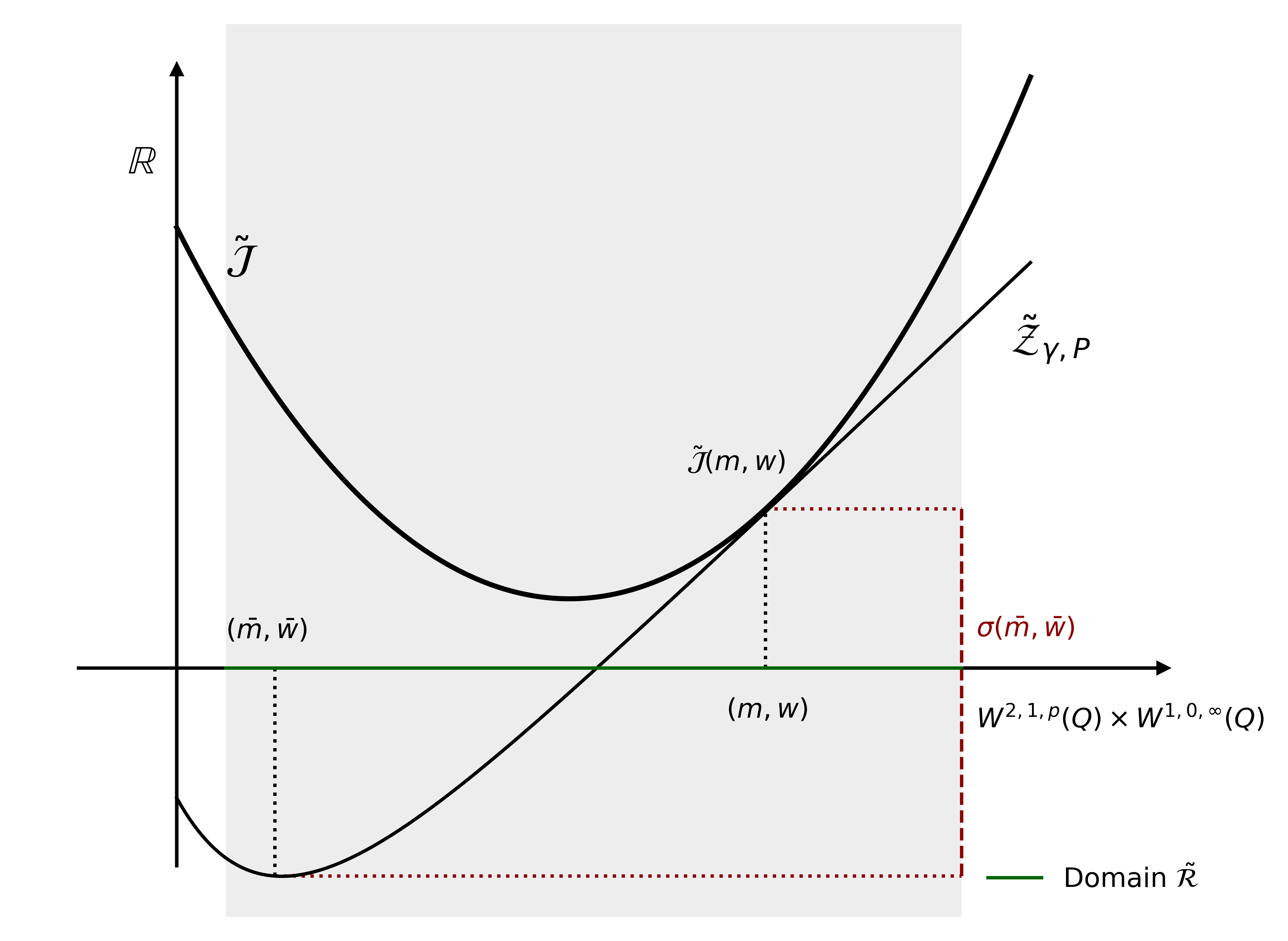
Figure 1: Illustration of the potential cost $\tilde{\mathcal{J}}$, the individual cost $\tilde{\mathcal{Z}}_{\gamma,P}$ and the exploitability $\sigma$.

We first justify the well-posedness of the algorithm (in particular, we need to justify the existence and uniqueness of $(m_{k},w_{k})$). To this goal, we introduce the following sequences

$$\begin{array}[]{llll}P_{k}(t)&=\phi(t,A\bar{w}_{k}(t)),&\gamma_{k}(x,t)&=f(x,t,\bar{m}_{k}(t)),\\ u_{k}(x,t)&=\mathsf{u}[\gamma_{k},P_{k}](x,t),&v_{k}(x,t)&=-\bm{H}_{p}[\nabla u_{k}+A^{\star}P_{k}]](x,t),\end{array}$$

for any $(x,t)\in Q$. For future reference, we define

$$\bar{v}_{k}=\bar{w}_{k}/\bar{m}_{k}.$$

In the next lemma, we provide an explicit formula to the minimization step, directly derived from Lemma 8.

Lemma 13.

For all $k\in\mathbb{N}$, we have $(m_{k},w_{k})=\chi(\mathsf{m}[v_{k}],v_{k})$. Moreover, there exists $\alpha_{k}\in(0,1)$ such that

$$\begin{cases}\begin{array}[]{rl}m_{k},\bar{m}_{k}\in&\mathcal{C}^{2+\alpha_{k},1+\alpha_{k}/2}(Q),\\ v_{k},w_{k},\bar{w}_{k}\in&\mathcal{C}^{1+\alpha_{k},\alpha_{k}}(Q;\mathbb{R}^{d}),\\ u_{k}\in&\mathcal{C}^{2+\alpha_{k},1+\alpha_{k}/2}(Q),\\ \gamma_{k}\in&\mathcal{C}^{\alpha_{k}}(Q),\\ P_{k}\in&\mathcal{C}^{\alpha_{k}}(0,T;\mathbb{R}^{k}).\end{array}\end{cases}$$ (20)

Proof.

We prove the result by induction. Let $k\in\mathbb{N}$. Assume that there exists $\alpha\in(0,1)$ such that $\bar{m}_{k}\in\mathcal{C}^{2+\alpha,1+\alpha/2}(Q)$, $\bar{w}_{k}\in\mathcal{C}^{1+\alpha,\alpha}(Q;\mathbb{R}^{d})$.

Step 1: $P_{k}\in\mathcal{C}^{\alpha}(0,T;\mathbb{R}^{k})$ and $\gamma_{k}\in\mathcal{C}^{\alpha}(Q)$. By assumptions (A6) and (A8),

$$|P_{k}(t_{2})-P_{k}(t_{1})| =|\phi[A\bar{w}_{k}](t_{2})-\phi[A\bar{w}_{k}](t_{1})|$$

$$\leq C\left(|t_{2}-t_{1}|^{\alpha}+|A\bar{w}_{k}(t_{2})-A\bar{w}_{k}(t_{1})|\right)$$

$$\leq C\left(|t_{2}-t_{1}|^{\alpha}+\|a\|_{L^{\infty}(Q;\mathbb{R}^{k\times d})}\int_{\mathbb{T}^{d}}|\bar{w}_{k}(t_{2})-\bar{w}_{k}(t_{1})|\mathrm{d}x\right),$$

for all $t_{1},t_{2}\in[0,T]$. It follows that $P_{k}$ is Hölder continuous, since by induction assumption, $\bar{w}_{k}\in\mathcal{C}^{1+\alpha,\alpha}(Q;\mathbb{R}^{d})$. The announced regularity on $\gamma_{k}$ is a direct consequence of the induction assumption ($\bar{m}_{k}\in\mathcal{C}^{2+\alpha,1+\alpha/2}(Q)$) and Assumption (A7).

Step 2: $u_{k}\in\mathcal{C}^{2+\alpha,1+\alpha/2}(Q)$. The regularity of $P_{k}$ and $\gamma_{k}$ obtained in the previous steps allows us to apply 3, which yields the announced regularity on $u_{k}$.

Step 3: $(m_{k},w_{k})=\chi(\mathsf{m}[v_{k}],v_{k})$. By Lemma 8 and Lemma 12, $\chi(\mathsf{m}[v_{k}],v_{k})$ is the unique minimizer of $\mathcal{Z}_{\gamma_{k},P_{k}}$, thus the unique minimizer of $h((\bar{m}_{k},\bar{w}_{k}),\cdot)$ on $\tilde{\mathcal{R}}$.

Step 4: $v_{k}\in\mathcal{C}^{1+\alpha,\alpha}(Q;\mathbb{R}^{d})$, $m_{k}\in\mathcal{C}^{2+\alpha,1+\alpha/2}(Q)$, and $w_{k}\in\mathcal{C}^{1+\alpha,\alpha}(Q;\mathbb{R}^{d})$. Direct consequence of the previous steps and Point 1 of Lemma 8.

Conclusion. By Step 4 and by the induction assumption, we have that $(\bar{m}_{k+1},\bar{w}_{k+1})\in\mathcal{C}^{2+\alpha,1+\alpha/2}(Q)\times\mathcal{C}^{1+\alpha,\alpha}(Q;\mathbb{R}^{d})$. Thus the induction assumption holds at $k+1$, which concludes the proof. ∎

Link with the fictitious play

Let us consider the primal-dual gap

$$\sigma_{k}=-\min_{(m,w)\in\tilde{\mathcal{R}}}h((\bar{m}_{k},\bar{w}_{k}),(m,w)).$$ (21)

As mentioned earlier, $\sigma_{k}$ is a primal gap certificate; it provides us with an upper bound of $\tilde{\mathcal{J}}(\bar{m}_{k},\bar{w}_{k})-\tilde{\mathcal{J}}(\bar{m},\bar{w})$ (this will be proved in Lemma 15). In the current mean field game context, it coincides with the notion of exploitability: it is the largest decrease in cost that a representative agent can reach by playing its best response, assuming that all other agents use the feedback $\bar{v}_{k}:=\bar{w}_{k}/\bar{m}_{k}$. Indeed, we have

$$\sigma_{k}=\ \tilde{\mathcal{Z}}_{\gamma_{k},P_{k}}(\bar{m}_{k},\bar{w}_{k})-\inf_{(m,w)\in\tilde{\mathcal{R}}}\tilde{\mathcal{Z}}_{\gamma_{k},P_{k}}(m,w)$$

$$=\ Z_{\gamma_{k},P_{k}}(\nu^{\bar{v}_{k}})-\inf_{\nu\in L_{\mathbb{F}}^{2}(t,T;\mathbb{R}^{d})}Z_{\gamma_{k},P_{k}}(\nu),$$

by Lemma 8 and Lemma 13.

We provide now an interpretation of the generalized gradient algorithm as a learning procedure called fictitious play. A definition and a study of the latter learning algorithm in the context of mean field games can be found in [16, 40]. Each iteration $k$ of Algorithm 1 relies on the following steps:

For $k\in\mathbb{N}$ let $(\bar{m}_{k},\bar{w}_{k})$ be a given belief and $\gamma_{k}$ and $P_{k}$ the resulting beliefs on congestion and price. Then there are four main steps:

1. Given $(\bar{m}_{k},\bar{w}_{k})$ compute the congestion terms $P_{k}$ and $\gamma_{k}$. In words, the agents make a prediction of the congestion term and the price at equilibrium, based on the belief $(\bar{m}_{k},\bar{w}_{k})$.

2. Find the value function $u_{k}$ solution to the Hamilton-Jacobi-Bellman equation parametrized by $(\gamma_{k},P_{k})$. Then compute the optimal control $v_{k}$, given the value function $u_{k}$ and the price $P_{k}$. This step can be interpreted as follows: for a given belief on the distributions of the others $(m_{k},w_{k})$, a representative agent computes its best response $v_{k}$.

3. Find the solution $m_{k}$ to the Fokker-Planck equation for the given drift $v_{k}$ and compute the associated distribution of controls $w_{k}$.

4. The actualization step of $(\bar{m}_{k+1},\bar{w}_{k+1})$ can be interpreted as a learning step. The learning rule consists in averaging the past realizations of the distribution and flow at a rate determined by the sequence $(\delta_{k})_{k\in\mathbb{N}}$.

6 Convergence Results

In this section, the generic constants $C$ and $\alpha$ depend on the data of the problem (introduced in Section 2.2) and depend on the pair $(\bar{m}_{0},\bar{w}_{0})$ chosen to initialize Algorithm 1.

Lemma 14.

There exists $C>0$ such that for any $k\in\mathbb{N}$,

$$\begin{array}[]{llll}\|\gamma_{k}\|_{W^{1,0,\infty}(Q;\mathbb{R}^{d})}&\leq C&\|m_{k}\|_{W^{2,1,p}(Q)}&\leq C\\ \|P_{k}\|_{L^{\infty}(0,T;\mathbb{R}^{k})}&\leq C&\|w_{k}\|_{W^{1,0,\infty}(Q;\mathbb{R}^{d})}&\leq C\\ \|u_{k}\|_{W^{2,1,p}(Q)}&\leq C&\|\bar{m}_{k}\|_{W^{2,1,p}(Q)}&\leq C\\ \|\nabla u_{k}\|_{W^{2,1,p}(Q;\mathbb{R}^{d})}&\leq C&\|\bar{w}_{k}\|_{W^{1,0,\infty}(Q;\mathbb{R}^{d})}&\leq C.\\ \|v_{k}\|_{W^{1,0,\infty}(Q;\mathbb{R}^{d})}&\leq C\\ \end{array}$$

In addition, we have

$$m_{k}(x,t)\geq 1/C,\quad\bar{m}_{k}(x,t)\geq 1/C,\quad\|\bar{v}_{k}\|_{L^{\infty}(Q;\mathbb{R}^{d})}\leq C,\quad$$

for all $(x,t)\in Q$.

Proof.

Let $k\in\mathbb{N}$. Assume that there exists $C>0$ such that the bounds hold for all $i\in\left\{0,\ldots,k-1\right\}$.

Step 1: Bounds of $\gamma_{k}$ and $P_{k}$. These bounds directly follow from assumptions (A4), (A5), and (A7). They imply the existence of $C>0$ such that

$$\|\gamma_{k}\|_{L^{\infty}(Q)}+\|\nabla\gamma_{k}\|_{L^{\infty}(Q;\mathbb{R}^{d})}+\|P_{k}\|_{L^{\infty}(0,T;\mathbb{R}^{k})}\leq C,$$

so that we can employ the technical Lemmas of Section 3 to prove the other announced bounds.

Step 2: Bounds of $u_{k}$ and $\nabla u_{k}$. Direct consequence of Step 1 and Lemma 3.

Step 3: Bounds of $v_{k}$, $m_{k}$ and $w_{k}$. Direct consequence of the previous steps and Point 2 of Lemma 8.

Step 4: Bounds of $\bar{m}_{k}$ and $\bar{w}_{k}$. This is a direct consequence of the fact that $(\bar{m}_{k},\bar{w}_{k})$ can be expressed as a convex combination of $(m_{k},w_{k})_{i=0,...,k-1}$ and $(\bar{m}_{0},\bar{w}_{0})$.

Step 5: $m_{k}(x,t),\bar{m}_{k}(x,t)\geq 1/C$ for any $(x,t)\in Q$. Since $m_{k}=\mathsf{m}[v_{k}]$ with $\|v_{k}\|_{W^{1,0,\infty}(Q;\mathbb{R}^{d})}\leq C$ and $m_{0}(x)\geq\varepsilon_{0}$ for any $x\in\mathbb{T}^{d}$, therefore $m_{k}(x,t)\geq 1/C$ by Lemma 29. Then $\bar{m}_{k}(x,t)\geq 1/C$ as a convex combination of $(m_{k})_{i=0,...,k-1}$.

Step 6: $\|\bar{v}_{k}\|_{L^{\infty}(Q;\mathbb{R}^{d})}\leq C$. By Step 4 and Step 5,

$$\|\bar{v}_{k}\|_{L^{\infty}(Q;\mathbb{R}^{d})}=\left\|\bar{w}_{k}/\bar{m}_{k}\right\|_{L^{\infty}(Q;\mathbb{R}^{d})}\leq C.$$

Conclusion. Since $(\bar{m}_{0},\bar{w}_{0})\in\mathcal{C}^{2+\alpha,1+\alpha/2}(Q)\times\mathcal{C}^{1+\alpha,\alpha}(Q;\mathbb{R}^{d})$ with $\bar{m}_{0}(x,t)>0$ for any $(x,t)\in Q$, the conclusion follows by induction. ∎

Recall the definition of the exploitability $\sigma_{k}$, given in (21). We define the sequence of primal gaps $(\epsilon_{k})_{k\in\mathbb{N}}$ as follows

$$\epsilon_{k}=\tilde{\mathcal{J}}(\bar{m}_{k},\bar{w}_{k})-\tilde{\mathcal{J}}(\bar{m},\bar{w}).$$

We recall that $(\bar{m},\bar{w})=\operatorname*{arg\,min}_{(m,w)\in\tilde{\mathcal{R}}}\tilde{\mathcal{J}}(m,w)$. The following Lemma is a certificate result, similar to inequality (18).

Lemma 15.

We have that $\epsilon_{k}\leq\sigma_{k}$.

Proof.

For any $(m,w)\in\tilde{\mathcal{R}}$ we have that

$$h((\bar{m}_{k},\bar{w}_{k}),(m,w))=\tilde{\mathcal{J}}(m,w)-\tilde{\mathcal{J}}(\bar{m}_{k},\bar{w}_{k})+a+b,$$

where

$$a =\int_{0}^{T}\bm{F}[\bar{m}_{k}]-\bm{F}[m]\mathrm{d}t+\int_{Q}f(x,t,\bar{m}_{k}(t))(m(x,t)-\bar{m}_{k}(x,t))\mathrm{d}x\mathrm{d}t\leq 0,$$

$$b =\int_{0}^{T}\bm{\Phi}[A\bar{w}_{k}]-\bm{\Phi}[Aw]\mathrm{d}t+\int_{0}^{T}\langle\phi(t,Aw_{k}(t)),A[w-\bar{w}_{k}](t)\rangle\mathrm{d}t\leq 0,$$

by convexity of $\bm{F}$ and $\bm{\Phi}$. Then we have that

$$\inf_{(m,w)\in\tilde{\mathcal{R}}}h((\bar{m}_{k},\bar{w}_{k}),(m,w))\leq\inf_{(m,w)\in\tilde{\mathcal{R}}}\tilde{\mathcal{J}}(m,w)-\tilde{\mathcal{J}}(\bar{m}_{k},\bar{w}_{k}),$$ (22)

and the conclusion follows. ∎

Lemma 16.

There exists $C>0$ such that for any $\delta\in[0,1]$, it holds:

$$\tilde{\mathcal{J}}(\bar{m}_{k}^{\delta},\bar{w}_{k}^{\delta})\leq\tilde{\mathcal{J}}(\bar{m}_{k},\bar{w}_{k})-\delta\sigma_{k}+\delta^{2}C,$$ (23)

where $(\bar{m}_{k}^{\delta},\bar{w}_{k}^{\delta})=\delta(m_{k},w_{k})+(1-\delta)(\bar{m}_{k},\bar{w}_{k})$.

Proof.

The convexity of $\tilde{L}$ yields

$$\int_{Q}\tilde{\bm{L}}[\bar{m}_{k}^{\delta},\bar{w}_{k}^{\delta}]\mathrm{d}x\mathrm{d}t\leq\int_{Q}\tilde{\bm{L}}[\bar{m}_{k},\bar{w}_{k}]+\delta\left(\tilde{\bm{L}}[\bar{m}_{k},\bar{w}_{k}]-\tilde{\bm{L}}[m_{k},w_{k}]\right)\mathrm{d}x\mathrm{d}t.$$ (24)

Using that $F$ is the primitive of $f$ in the sense of (2), we have for all $t\in[0,T]$,

$$\bm{F}[\bar{m}^{\delta}_{k}](t)=\bm{F}[\bar{m}_{k}](t)$$

$$+\delta_{k}\int_{0}^{1}\int_{\mathbb{T}^{d}}f\left(x,t,\bar{m}_{k}(t)+s\delta(m_{k}(t)-\bar{m}_{k}(t))\right)(m_{k}(x,t)-\bar{m}_{k}(x,t))\mathrm{d}x\mathrm{d}s,$$ (25)

For any $(x,t)\in Q$, the Lipschitz-continuity of $f$ yields

$$f\left(x,t,\bar{m}_{k}(t)+s\delta(m_{k}(t)-\bar{m}_{k}(t))\right) \leq f(x,t,\bar{m}_{k}(t))+s\delta C\|m_{k}(t)-\bar{m}_{k}(t)\|_{L^{2}(\mathbb{T}^{d})}$$

$$\leq f(x,t,\bar{m}_{k}(t))+s\delta C,$$

since $\bar{m}_{k},m_{k}$ are uniformly bounded by Lemma 14. Plugging into (25) yields

$$\bm{F}[\bar{m}^{\delta}_{k}](t)=\bm{F}[\bar{m}_{k}](t)+\delta\int_{\mathbb{T}^{d}}f(x,t,\bar{m}_{k}(t))(m_{k}(x,t)-\bar{m}_{k}(x,t))\mathrm{d}x+\delta^{2}C.$$ (26)

Now using that $\Phi$ is the primitive of $\phi$, we have

$$\bm{\Phi}[A\bar{w}^{\delta}_{k}](t)\leq\bm{\Phi}[A\bar{w}_{k}](t)+\delta\langle\phi(t,A\bar{w}_{k}(t)),A[w_{k}-\bar{w}_{k}](t)\rangle+\delta^{2}|A[w_{k}-\bar{w}_{k}](t)|^{2}$$

by Assumption (A8). Using that $\bar{w}_{k},w_{k}$ are uniformly bounded by Lemma 14 yields

$$|A[w_{k}-\bar{w}_{k}](t)|\leq\|a(t)\|_{L^{\infty}(\mathbb{T}^{d})}\|w_{k}(t)-\bar{w}_{k}(t)\|_{L^{\infty}(\mathbb{T}^{d})}\leq C.$$

Combining the two last inequalities yields

$$\bm{\Phi}[A\bar{w}^{\delta}_{k}](t)\leq\bm{\Phi}[A\bar{w}_{k}](t)+\delta\langle\phi(t,A\bar{w}_{k}(t)),A[w_{k}-\bar{w}_{k}](t)\rangle+\delta^{2}C.$$ (27)

Then inequality (23) holds combining the Assumption (A9) on $g$ and inequalities (24), (26), and (27) which concludes the proof. ∎

Lemma 17.

We have that

$$\epsilon_{k+1}\leq(1-\delta_{k})\epsilon_{k}+\delta_{k}^{2}C.$$

Proof.

A direct application of Lemma 16 yields,

$$\tilde{\mathcal{J}}(\bar{m}_{k+1},\bar{w}_{k+1})\leq\tilde{\mathcal{J}}(\bar{m}_{k},\bar{w}_{k})-\delta_{k}\sigma_{k}+\delta_{k}^{2}C.$$

Thus $\epsilon_{k+1}\leq\epsilon_{k}-\delta_{k}\sigma_{k}+\delta_{k}^{2}K$ and the conclusion follows by Lemma 15 since $-\sigma_{k}\leq-\epsilon_{k}$. ∎

Lemma 18.

Let $L_{0}\coloneqq\max\{\epsilon_{0}/2,C\}$ and $L_{1}\coloneqq\max\{2\epsilon_{1},C\}/\ln(2)$. We have that

$$\begin{cases}\begin{array}[]{llll}{\text{(i)}}&\epsilon_{k}\leq\frac{4L_{0}}{k+2}&{\text{if }}\delta_{k}=\frac{2}{k+2},&{\text{for any }}k\in\mathbb{N},\\[10.00002pt] {\text{(ii)}}&\epsilon_{k}\leq\frac{\ln(k+1)L_{1}}{k+1}&{\text{if }}\delta_{k}=\frac{1}{k+1},&{\text{for any }}k\in\mathbb{N}\setminus\{0\}.\end{array}\end{cases}$$ (28)

The above Lemma summarizes the rate of convergence of the sequence $(\epsilon_{k})_{k\in\mathbb{N}}$ for two learning rates. The first result (28,i) is classical in the context of conditional gradient algorithm (see [25, 29]). For the sake of completeness we recall how to derive this result in the following proof. The second result (28,ii) corresponds to the classical fictitious play learning rate.

Proof.

Step 1: (28,i) holds. Let $\delta_{k}=2/(k+2)$ for any $k\in\mathbb{N}$. For $k=0$, it is clear that (28,i) holds. For $k>0$, assume that $\epsilon_{k}$ satisfies the inequality (28,i). By Lemma 17 we have that

$$\epsilon_{k+1}\leq\left(1-\frac{2}{k+2}\right)\frac{4L_{0}}{k+2}+\frac{4C}{(k+2)^{2}}\leq\frac{4L_{0}(k+1)}{(k+2)^{2}}\leq\frac{4L_{0}}{(k+3)},$$

and by induction the step $1$ is proved.

Step 2: (28,ii) holds. Let $\delta_{k}=1/(k+1)$ for any $k\in\mathbb{N}$. For $k=1$, it is clear that (28,ii) holds by Lemma 17. For $k>1$ assume that $\epsilon_{k}$ satisfies the inequality (28,ii) then by Lemma 17 we have

$$\epsilon_{k+1}\leq\left(1-\frac{1}{k+1}\right)\frac{\ln(k+1)L_{1}}{k+1}+\frac{C}{(k+1)^{2}}.$$

Then to prove (28,ii) it is enough to check

$$\frac{k\ln(k+1)L_{1}+C}{(k+1)^{2}}\leq\frac{\ln(k+2)}{(k+2)}.$$

Multiplying both side by $(k+1)^{2}(k+2)$, the inequation (28,ii) holds if

$$(k+2)\frac{C}{L_{1}} \leq(k+1)^{2}\ln(k+2)-k(k+2)\ln(k+1)$$

$$\leq k(k+2)\ln\left(1+\frac{1}{k+1}\right)+\ln(k+2).$$ (29)

The concavity of the logarithm yields $\ln\left(1+1/(k+1)\right)\geq\ln(2)/k$. Thus the inequality (29) holds whenever

$$\frac{C}{L_{1}}\leq\ln(2)+\frac{\ln(k+2)}{k+2},$$

which holds by definition of $L_{1}$. Then Step 2 is proved, which concludes the proof. ∎

Lemma 19.

There exists $C>0$ such that $\sigma_{k}\leq C\epsilon_{k}^{1/2}$ for all $k\in\mathbb{N}$.

Proof.

For any $\delta\in[0,1]$, Lemma 16 yields $\tilde{\mathcal{J}}(\bar{m},\bar{w})\leq\tilde{\mathcal{J}}(\bar{m}_{k},\bar{w}_{k})-\delta\sigma_{k}+\delta^{2}C$. It follows that

$$\sigma_{k}\leq\epsilon_{k}/\delta+\delta C,\qquad\forall\delta\in(0,1],$$ (30)

by Lemma 18. The optimal choice of $\delta\in(0,1]$ in the latter inequality is given by $\delta=\min\{\sqrt{\epsilon_{k}/C},1\}$. Since the sequence $(\epsilon_{k})_{k\in\mathbb{N}}$ is uniformly bounded from above, we can increase the constant $C$, so that one can choose $\delta=\sqrt{\epsilon_{k}/C}\in(0,1]$. For this choice of $\delta$, inequality (30) yields the announced result. ∎

For any $k\in\mathbb{N}$ we denote

$$\begin{array}[]{llllll}\delta\bar{m}_{k}&=\bar{m}_{k}-\bar{m},&\delta\bar{w}_{k}&=\bar{w}_{k}-\bar{w},&\delta\bar{v}_{k}&=\bar{v}_{k}-\bar{v},\\ \delta P_{k}&=P_{k}-\bar{P},&\delta\gamma_{k}&=\gamma_{k}-\bar{\gamma},&\delta u_{k}&=u_{k}-\bar{u}.\end{array}$$

Theorem 20.

There exists $C>0$ such that for all $k\in\mathbb{N}$,

$$\|\delta\bar{v}_{k}\|_{L^{2}(Q;\mathbb{R}^{d})}+\|\delta\bar{m}_{k}\|_{L^{\infty}(0,T;L^{2}(\mathbb{T}^{d}))}+\|\delta\bar{w}_{k}\|_{L^{2}(Q;\mathbb{R}^{d})}$$

$$+\|\delta P_{k}\|_{L^{2}(0,T;\mathbb{R}^{k})}+\|\delta\gamma_{k}\|_{L^{\infty}(Q)}+\|\delta u_{k}\|_{L^{\infty}(Q)} \leq C\epsilon^{1/2}_{k}.$$

Proof.

Step 1: $\|\delta\bar{v}_{k}\bar{m}_{k}\|_{L^{2}(Q;\mathbb{R}^{d})}\leq C\epsilon_{k}^{1/2}$. By Lemma 10, we have

$$\frac{1}{C}\int_{Q}|\delta\bar{v}_{k}|^{2}\bar{m}_{k}\mathrm{d}x\mathrm{d}t\leq\mathcal{J}(\bar{m}_{k},\bar{v}_{k})-\mathcal{J}(\bar{m},\bar{v})=\epsilon_{k}.$$

Combining the above inequality with $\|\bar{m}_{k}\|_{L^{\infty}(Q)}\leq C$ yields the desired estimate.

Step 2: $\|\delta\bar{v}_{k}\|_{L^{2}(Q;\mathbb{R}^{d})}\leq C\epsilon_{k}^{1/2}$. By Step 1 and Lemma 14,

$$\|\delta\bar{v}_{k}\|_{L^{2}(Q;\mathbb{R}^{d})}\leq\|\delta\bar{v}_{k}\bar{m}_{k}\|_{L^{2}(Q;\mathbb{R}^{d})}\|1/\bar{m}_{k}\|_{L^{\infty}(Q)}\leq C\epsilon_{k}^{1/2},$$

and Step 2 holds.

Step 3: $\|\delta\bar{m}_{k}\|_{C(0,T;L^{2}(\mathbb{T}^{d}))}\leq C\epsilon^{1/2}_{k}$. We have that $\delta\bar{m}_{k}$ satisfies

$$\begin{array}[]{rlr}\partial_{t}\delta\bar{m}_{k}-\Delta\delta\bar{m}_{k}+\nabla\cdot(\bar{v}\delta\bar{m}_{k})=&-\nabla\cdot(\delta\bar{v}_{k}\bar{m}_{k}),&(x,t)\in Q,\\ \delta m_{k}(0,x)=&0,&x\in\mathbb{T}^{d}.\end{array}$$

We define the space $V=W^{2,1}(\mathbb{T}^{d})$ and its dual $V^{*}$. Then $\delta m_{k}$ is solution of a parabolic equation of the form

$$\begin{array}[]{rlr}\partial_{t}m(t)+B(t)m(t)=&f(t),&(x,t)\in Q,\\ m(0,x)=&0,&x\in\mathbb{T}^{d},\end{array}$$

where $B(t)\in L(V,V^{*})$ and $f(t)\in V^{*}$. It is easy to verify that since $\bar{v}\in W^{1,0,\infty}(Q;\mathbb{R}^{d})$, there exists a constant $C$ such that $\langle B(t)y,y^{\prime}\rangle_{V}\leq C\|y\|_{V}\|y^{\prime}\|_{V}$, for a.e. $t\in(0,T)$ and for all $y$ and $y^{\prime}$ in $V$. For any $y\in V$ we further have that

$$\langle B(t)y,y\rangle_{V} =\int_{\mathbb{T}^{d}}\left(-\Delta y+\nabla\cdot\bar{v}(t)y+\langle\bar{v}(t),\nabla y\rangle\right)y\mathrm{d}x$$

$$\geq\int_{\mathbb{T}^{d}}|\nabla y|^{2}+C|y|^{2}-C|\nabla y||y|\mathrm{d}x\geq\frac{1}{2}\|y\|^{2}_{V}-\frac{C}{2}\|y\|^{2}_{L^{2}(\mathbb{T}^{d})},$$

where we have used that $-\int_{\mathbb{T}^{d}}|\nabla y||y|\mathrm{d}x\geq-\frac{1}{2}\int_{\mathbb{T}^{d}}|\nabla y|^{2}/C+C|y|^{2}\mathrm{d}x$. Then $B(t)$ is semi-coercive, uniformly in time. Thus by [50, Chapter 3, Theorem 1.2] we have

$$\|\delta\bar{m}_{k}\|_{L^{2}(0,T;V)}+\|\partial_{t}\delta\bar{m}_{k}\|_{L^{2}(0,T;V^{*})} \leq C\|f\|_{L^{2}(0,T;V^{*})}$$

$$\leq C\|\nabla\cdot\delta\bar{v}_{k}\bar{m}_{k}\|_{L^{2}(0,T;V^{*})}$$

$$\leq C\|\delta\bar{v}_{k}\bar{m}_{k}\|_{L^{2}(Q;\mathbb{R}^{d})}\leq C\epsilon^{1/2}_{k}.$$

We conclude Step 3 with the continuous inclusion (see [50, Chapter 3, Theorem 1.1])

$$\{m\in L^{2}(0,T;V);\;\partial_{t}m\in L^{2}(0,T;V^{*})\}\subseteq C(0,T;L^{2}(\mathbb{T}^{d})).$$

Step 4: $\|\delta\bar{w}_{k}\|_{L^{2}(Q;\mathbb{R}^{d})}\leq C\epsilon^{1/2}_{k}$. By definition of $\delta\bar{w}_{k}$ we have

$$\|\delta\bar{w}_{k}\|_{L^{2}(Q;\mathbb{R}^{d})}\leq\|\delta\bar{v}_{k}\bar{m}_{k}\|_{L^{2}(Q;\mathbb{R}^{d})}+\|\bar{v}\delta\bar{m}_{k}\|_{L^{2}(Q;\mathbb{R}^{d})}\leq C\epsilon^{1/2}_{k},$$

where the last inequality follows from Step 1 and Step 3.

Step 5: $\|\delta P_{k}\|_{L^{2}(0,T;\mathbb{R}^{k})}\leq C\epsilon^{1/2}_{k}$ and $\|\delta\gamma_{k}\|_{L^{\infty}(Q)}\leq C\epsilon^{1/2}_{k}$. Using that $\phi$ is Lipschitz with respect to its second variable (see Assumption (A8)),

$$|\delta P_{k}(t)|=|\phi(t,A\bar{w}_{k}(t))-\phi(t,A\bar{w}(t))| \leq C|A\delta\bar{w}_{k}(t)|$$

for almost every $t\in[0,T]$. Since

$$|A\delta\bar{w}_{k}(t)|=\left|\int_{\mathbb{T}^{d}}a(x,t)\delta\bar{w}_{k}(x,t)\mathrm{d}x\right|\leq\|a(t)\|_{L^{\infty}(\mathbb{T}^{d};\mathbb{R}^{k\times d})}\|\delta\bar{w}_{k}(t)\|_{L^{1}(\mathbb{T}^{d};\mathbb{R}^{d})},$$

Since $\|a\|_{L^{\infty}(Q;\mathbb{R}^{k\times d})}\leq C$, Step 4 yields the desired estimate

$$\|\delta P_{k}\|_{L^{2}(0,T;\mathbb{R}^{k})}\leq C\|\delta\bar{w}_{k}\|_{L^{2}(Q;\mathbb{R}^{d})}\leq C\epsilon^{1/2}_{k}.$$

Using that $f$ is Lipschitz with respect to its third variable (see Assumption (A7)) yields

$$|\delta\gamma_{k}(x,t)|=|f(x,t,\bar{m}_{k}(t))-f(x,t,\bar{m}(t))|\leq C\|\delta\bar{m}_{k}(t)\|_{L^{2}(\mathbb{T}^{d})},$$

for any $(x,t)\in Q$. Taking the supremum over $(x,t)\in Q$ both sides of the inequality yields that $\|\delta\gamma_{k}\|_{C(Q)}\leq C\epsilon^{1/2}_{k}$ by Step 3, which concludes the step.

Step 6: $\|\delta u_{k}\|_{C(Q)}\leq C\epsilon^{1/2}_{k}$. Since $\|\gamma_{k}\|_{L^{\infty}(Q)}\leq C$, $\|P_{k}\|_{L^{2}(0,T;\mathbb{R}^{k})}\leq C$, $\|\bar{\gamma}\|_{L^{\infty}(Q)}\leq C$, and $\|\bar{P}\|_{L^{2}(0,T;\mathbb{R}^{k})}\leq C$, Lemma 2 yields

$$\delta u_{k}(x,t)=\inf_{\alpha\in L_{\mathbb{F}}^{2,C}(t,T;\mathbb{R}^{d})}J_{\gamma_{k},P_{k}}(x,t,\alpha)-\inf_{\alpha^{\prime}\in L_{\mathbb{F}}^{2,C}(t,T;\mathbb{R}^{d})}J_{\bar{\gamma},\bar{P}}(x,t,\alpha^{\prime}),$$

for any $(x,t)\in Q$. We denote $(X^{\alpha}_{s})_{s\in[t,T]}$ the solution to the stochastic differential equation $\mathrm{d}X_{s}=\alpha_{s}\mathrm{d}s+\sqrt{2}\mathrm{d}B_{s}$ with $X^{\alpha}_{t}=x$, for any $\alpha\in L_{\mathbb{F}}^{2}(t,T;\mathbb{R}^{d})$. Then

$$|\delta u_{k}(x,t)| \leq\sup_{\alpha\in L_{\mathbb{F}}^{2,C}(t,T;\mathbb{R}^{d})}|J_{\gamma_{k},P_{k}}(x,t,\alpha)-J_{\bar{\gamma},\bar{P}}(x,t,\alpha)|$$

$$\leq\sup_{\alpha\in L_{\mathbb{F}}^{2,C}(t,T;\mathbb{R}^{d})}\mathbb{E}\left[\int_{t}^{T}|\langle A^{\star}[\delta P_{k}](X^{\alpha}_{s},s),\alpha_{s}\rangle|+|\delta\gamma_{k}(X^{\alpha}_{s},s)|\mathrm{d}s\right].$$

For any $(x,s)\in Q$ and $\alpha\in\mathbb{R}^{d}$, the Cauchy-Schwarz inequality yields

$$|\langle A^{\star}[\delta P_{k}](x,s),\alpha\rangle| \leq|\langle a(x,s)\delta P_{k}(s)||\alpha|$$

$$\leq\|a\|_{L^{\infty}(Q;\mathbb{R}^{k\times d})}|\delta P_{k}(s)||\alpha|.$$

Since $\|a\|_{L^{\infty}(Q;\mathbb{R}^{k\times d})}\leq C$, we finally have

$$|\delta u_{k}(x,t)|\leq C\left(\|\delta P_{k}\|_{L^{2}(0,T;\mathbb{R}^{k})}+\|\delta\gamma_{k}\|_{L^{\infty}(Q)}\right).$$

Thus Step 6 holds by Step 5, which concludes the proof. ∎

Let us comment our last convergence results: Lemma 19 and Theorem 20. For the fictitious play learning rate $\delta_{k}=1/(k+1)$, we have proved that the primal gap sequence $(\epsilon_{k})_{k\in\mathbb{N}}$ converges in $O(\ln(k)/k)$ and the exploitability sequence $(\sigma_{k})_{k\in\mathbb{N}}$ and the sequence of variables $(\bar{m}_{k},\bar{w}_{k},\bar{v}_{k},P_{k},\gamma_{k},u_{k})_{k\in\mathbb{N}}$ converge in $O(\sqrt{\ln(k)/k})$. We have obtained a sharper convergence result for the Frank-Wolfe learning rate $\delta_{k}=2/(k+2)$. For this choice, we have shown that the primal gap sequence $(\epsilon_{k})_{k\in\mathbb{N}}$ converges in $O(1/k)$ and the exploitability sequence $(\sigma_{k})_{k\in\mathbb{N}}$ and the sequence of variables $(\bar{m}_{k},\bar{w}_{k},\bar{v}_{k},P_{k},\gamma_{k},u_{k})_{k\in\mathbb{N}}$ converge in $O(\sqrt{1/k})$. The convergence results for $(\bar{m}_{k},\bar{w}_{k},\bar{v}_{k},P_{k},\gamma_{k},u_{k})$ are new in the mean field game literature.

We conclude this section with a discussion on our results. The results concerning the convergence of the primal gap and the exploitability (Lemmas 18 and 19) are the same as those obtained in [31] for different mean field game models, with a discrete structure. These results are indeed general, since they only rely on the convexity structure of the potential problem and the regularity properties of the coupling terms. Therefore, they could certainly be adapted to other models, for example first order mean field games.

We also expect that similar convergence results, for the coupling terms, the value function, and the distribution, could be obtained in a different framework. A key step in the proof would be to establish a quadratic growth property (as the one obtained in Lemma 10), under a strong convexity assumption on the running cost $L$.

Appendix A Regularity of the Hamiltonian

Some properties of the Hamiltonian can be deduced from the convexity assumption (A1) and the Hölder continuity of $L$ and its derivatives (Assumption (A6)). They are collected in the following lemmas. whose proofs can be found in [9].

Lemma 21.

The Hamiltonian $H$ is differentiable with respect to $p$ and $H_{p}$ is differentiable with respect to $x$ and $p$. Moreover, for all $R>0$, there exists $\alpha\in(0,1)$ such that $H\in\mathcal{C}^{\alpha}(B_{R})$, $H_{p}\in\mathcal{C}^{\alpha}(B_{R},\mathbb{R}^{d})$, $H_{px}\in\mathcal{C}^{\alpha}(B_{R},\mathbb{R}^{d\times d})$, and $H_{pp}\in\mathcal{C}^{\alpha}(B_{R},\mathbb{R}^{d\times d})$.

Proof.

See [9, Lemma 1]. ∎

Lemma 22.

There exists a constant $C>0$ such that for all $(x,t)\in Q$, for all $p\in\mathbb{R}^{d}$ and for all $v\in\mathbb{R}^{d}$,

$$H(x,t,p)+L(x,t,v)+\langle p,v\rangle\geq\frac{1}{C}|v+H_{p}(x,t,p)|^{2}.$$ (31)

In addition for any $m,\bar{m}\geq 0$ and $\bar{v}=-H_{p}(x,t,p)$ we have that

$$L(x,t,v)m-L(x,t,\bar{v})\bar{m}\geq-H(x,t,p)(m-\bar{m})-\langle p,w-\bar{w}\rangle+\frac{1}{C}|v-\bar{v}|^{2}m,$$ (32)

where $(w,\bar{w})\coloneqq(mv,\bar{m}\bar{v})$.

Proof.

See [9, Proof of Proposition 2]. ∎

Appendix B A priori bounds for parabolic equations

In this appendix we provide estimates for the following parabolic equation:

$$\begin{array}[]{rlr}\partial_{t}u-\sigma\Delta u+\langle b,\nabla u\rangle+cu=&h,&(x,t)\in Q,\\ u(x,0)=&u_{0}(x),&x\in\mathbb{T}^{d},\end{array}$$ (33)

for different assumptions on $b$, $c$, $h$, and $u_{0}$. The proofs of the following results can be found in the Appendix of [9]; they largely rely on [46]. We recall that $p$ is a fixed parameter and $p>d+2$.

Theorem 23.

For all $R>0$, there exists $C>0$ such that for all $u_{0}\in W^{p,2-2/p}(\mathbb{T}^{d})$, for all $b\in L^{p}(Q;\mathbb{R}^{d})$, for all $c\in L^{p}(Q)$, for all $h\in L^{p}(Q)$, satisfying

$$\|u_{0}\|_{W^{p,2-2/p}(\mathbb{T}^{d})}\leq R,\quad\|b\|_{L^{p}(Q;\mathbb{R}^{d})}\leq R,\quad\|c\|_{L^{p}(Q)}\leq R,\quad\|h\|_{L^{p}(Q)}\leq R,$$

equation (33) has a unique solution $u$ in $W^{2,1,p}(Q)$. Moreover, $\|u\|_{W^{2,1,p}(Q)}\leq C$.

Theorem 24.

For $q\in(1,\infty)$, the trace at time $t=0$ of elements of $W^{2,1,q}(Q)$ belongs to $W^{q,2-2/q}(\Omega)$.

Theorem 25.

There exists $C>0$ such that for all $u_{0}\in W^{2-2/p,p}(\mathbb{T}^{d})$ and for all $h\in L^{p}(Q)$, the unique solution $u$ to (33) (with $b=0$ and $c=0$) satisfies the following estimate:

$$\|u\|_{W^{2,1,p}(Q)}\leq C\left(\|u_{0}\|_{W^{2-2/p,p}(\mathbb{T}^{d})}+\|h\|_{L^{p}(Q)}\right).$$

Lemma 26.

There exists $\delta\in(0,1)$ and $C>0$ such that for all $u\in W^{2,1,p}(Q)$,

$$\|u\|_{\mathcal{C}^{\delta}(Q)}+\|\nabla u\|_{\mathcal{C}^{\delta}(Q;\mathbb{R}^{d})}\leq C\|u\|_{W^{2,1,p}(Q)}.$$

Theorem 27.

For all $\beta\in(0,1)$, for all $R>0$, there exist $\alpha\in(0,1)$ and $C>0$ such that for all $u_{0}\in\mathcal{C}^{2+\beta}(\mathbb{T}^{d})$, $b\in\mathcal{C}^{\beta,\beta/2}(Q;\mathbb{R}^{d})$, $c\in\mathcal{C}^{\beta,\beta/2}(Q)$ and $h\in\mathcal{C}^{\beta,\beta/2}(Q)$ satisfying

$$\|u_{0}\|_{\mathcal{C}^{2+\beta}(\mathbb{T}^{d})}\leq R,\ \ \|b\|_{\mathcal{C}^{\beta,\beta/2}(Q;\mathbb{R}^{d})}\leq R,\ \ \|c\|_{\mathcal{C}^{\beta,\beta/2}(Q)}\leq R,\ \ \text{and}\ \ \|h\|_{\mathcal{C}^{\beta,\beta/2}(Q)}\leq R,$$

the solution to (33) lies in $\mathcal{C}^{2+\alpha,1+\alpha/2}(Q)$ and satisfies $\|u\|_{\mathcal{C}^{2+\alpha,1+\alpha/2}(Q)}\leq C$.

Appendix C Maximum principle

In this appendix we establish a maximum principle for the Fokker-Planck equation. We study the parabolic equation (33) with $h=0$,

$$\begin{array}[]{rlr}\partial_{t}m-\sigma\Delta m+\langle b,\nabla m\rangle+cm=&0,&(x,t)\in Q,\\ m(x,0)=&m_{0}(x),&x\in\mathbb{T}^{d}.\end{array}$$ (34)

We assume that $m_{0}$ satisfies Assumption (A9) and define the mapping $\bar{\mathsf{m}}\colon L^{\infty}(Q;\mathbb{R}^{d})\times L^{\infty}(Q)\to W^{2,1,p}(Q)$ which associates to any $(b,c)$ the solution to (34). By Theorem 23 the mapping $\bar{\mathsf{m}}$ is well-defined.

Lemma 28.

The mapping $\bar{\mathsf{m}}$ is continuous.

Proof.

Consider the mapping $\varphi:W^{2,1,p}(Q)\times L^{\infty}(Q;\mathbb{R}^{d})\times L^{\infty}(Q)\to W^{p,2-2/p}(\mathbb{T}^{d})\times L^{p}(Q)$ defined by

$$\varphi[m,b,c]=(m(0,\cdot)-m_{0}(\cdot),\partial_{t}m-\sigma\Delta m+\langle b,\nabla m\rangle+cm).$$

We define

$$\begin{array}[]{llll}\varphi_{0}[m]&=m(0,\cdot),&\varphi_{2}[m,b]&=\langle b,\nabla m\rangle,\\ \varphi_{1}[m]&=\partial_{t}m-\sigma\Delta m,&\varphi_{3}[m,c]&=cm,\end{array}$$

so that $\varphi[m,b,c]=(\varphi_{0}[m]-m_{0}(\cdot),\varphi_{1}[m]+\varphi_{2}[m,b]+\varphi_{3}[m,c])$. By Theorem 23 and Theorem 24, there exists a constant $C>0$ such that

$$\begin{array}[]{llll}\|\varphi_{0}[m]\|_{W^{p,2-2/p}(\mathbb{T}^{d})}\!\!&\leq C\|m\|_{W^{2,1,p}(Q)},&\|\varphi_{2}[m,b]\|_{L^{p}(Q)}\!\!\!\!&\leq\|b\|_{L^{\infty}(Q)}\|m\|_{W^{2,1,p}(Q)},\\ \|\varphi_{1}[m]\|_{L^{p}(Q)}&\leq C\|m\|_{W^{2,1,p}(Q)},&\|\varphi_{3}[m,c]\|_{L^{p}(Q)}\!\!\!\!&\leq\|c\|_{L^{\infty}(Q)}\|m\|_{W^{2,1,p}(Q)}.\end{array}$$

Thus $\varphi_{0}$ and $\varphi_{1}$ (resp. $\varphi_{2}$ and $\varphi_{3}$) are $C^{\infty}$ as bounded linear (resp. bi-linear) applications. It follows that $\varphi$ is $C^{\infty}$. Let $(m,b,c)\in W^{2,1,p}(Q)\times L^{p}(Q;\mathbb{R}^{d})\times L^{p}(Q)$ be such that $\varphi[m,b,c]=0$. For any direction $z\in W^{2,1,p}(Q)$, we have

$$D_{m}\varphi[m,b,c]z=(z(0,\cdot),\partial_{t}z-\sigma\Delta z+\langle b,\nabla z\rangle+cz).$$

For any $(h_{0},h_{1})\in W^{p,2-2/p}(\mathbb{T}^{d})\times L^{p}(Q)$, the equation

$$\begin{array}[]{rlr}\partial_{t}z-\sigma\Delta z+\langle b,\nabla z\rangle+cz=&h_{1},&(x,t)\in Q,\\ z(x,0)=&h_{0},&x\in\mathbb{T}^{d},\end{array}$$

has a unique solution $z\in W^{2,1,p}(Q)$, by Theorem 23. Then $D_{m}\varphi[m,b,c]$ is bijective and thus invertible. The conclusion follows by the implicit function theorem. ∎

Lemma 29.

Let $v\in W^{1,0,\infty}(Q;\mathbb{R}^{d})$ and let $m=\bar{\mathsf{m}}[v,\nabla\cdot v]\in W^{2,1,p}(Q)$ be the solution to (34) with $(b,c)=(v,\nabla\cdot v)$. Assume that $m_{0}(x)\geq\varepsilon_{0}>0$ for any $x\in\mathbb{T}^{d}$. Then

$$m(x,t)\geq\varepsilon_{0}\exp\big{(}-T\|\nabla\cdot v\|_{L^{\infty}(Q)}\big{)},\quad\forall(x,t)\in Q.$$ (35)

Proof.

We first prove the result when $v\in\mathcal{C}^{1+\alpha,\alpha/2}(Q;\mathbb{R}^{d})$, for some $\alpha\in(0,1)$. By Theorem 27, $m\in C^{2,1}(Q)$. Let $\kappa>\|\nabla\cdot v\|_{L^{\infty}(Q)}$. We define

$$y(x,t)=e^{-\kappa t}\left(m(x,t)-\varepsilon_{0}e^{-\kappa t}\right),$$

for all $(x,t)\in Q$. By a direct computation we have

$$\partial_{t}y(x,t)=-y(x,t)(\kappa-\nabla\cdot v(x,t))+\Delta y(x,t)+\langle v(x,t),\nabla y(x,t)\rangle$$

$$+\varepsilon_{0}e^{-2\kappa t}\left(\kappa+\nabla\cdot v(x,t)\right).$$ (36)

Next we show that $y(x,t)\geq 0$ for all $(x,t)\in Q$. Let $(x_{0},t_{0})\in\operatorname*{arg\,min}_{(x,t)\in Q}y(x,t)$. Let us assume, by a way of contradiction, that $y(x_{0},t_{0})<0$. Since $y(0,x)\geq 0$ for any $x\in\mathbb{T}^{d}$, we have that $t_{0}>0$ and thus $\partial_{t}y(x_{0},t_{0})\leq 0$. Since $x_{0}\in\mathbb{T}^{d}$, we have that $\nabla y(x_{0},t_{0})=0$. Moreover, since $m$ is twice differentiable with respect to its second variable, we have that $\Delta y(x_{0},t_{0})\geq 0$. Then it follows from (36) that

$$\partial_{t}y(x_{0},t_{0})\geq-y(x_{0},t_{0})(\kappa-\nabla\cdot v(x_{0},t_{0}))\\ +\varepsilon_{0}e^{-2\kappa t_{0}}\left(\kappa+\nabla\cdot v(x_{0},t_{0})\right).$$

The right-hand side is positive since $\kappa>\|\nabla\cdot v\|_{L^{\infty}(Q)}$. This contradicts the inequality $\partial_{t}y(x_{0},t_{0})\leq 0$ and proves that $y(x,t)\geq 0$, for any $(x,t)\in Q$. It follows then from the definition of $y$ that $m(x,t)\geq\varepsilon_{0}e^{-\kappa t}$, for any $(x,t)\in Q$. Passing to the limit when $\kappa\rightarrow$ yields (35).

We now consider the general case when $v\in W^{1,0,\infty}(Q;\mathbb{R}^{d})$ and proceed by density. Let $(\rho_{k})_{k\in\mathbb{N}}$ be a sequence of regularizing kernels in $C^{\infty}(Q)$. We define $v_{k}=\rho_{k}*v\in C^{\infty}(Q;\mathbb{R}^{d})$, where $*$ is the convolution product. We next define $m_{k}=\bar{\mathsf{m}}[v_{k},\nabla\cdot v_{k}]$ for any $k\in\mathbb{N}$. Applying (35) to $m_{k}$, we obtain that

$$m_{k}(x,t)\geq\varepsilon_{0}\exp\big{(}-T\|\nabla\cdot v_{k}\|_{L^{\infty}(Q)}\big{)},\quad\forall(x,t)\in Q.$$

Since $v_{k}$ (resp. $\nabla v_{k}$) uniformly converges to $v$ (resp. $\nabla v$) and since $\bar{\mathsf{m}}$ is continuous for the uniform topology, we deduce that $m_{k}$ converges to $m$ in $W^{2,1,p}(Q)$ and finally that $m_{k}$ uniformly converges to $m$, by Lemma 26. This allows us to pass to the limit in the above inequality, which concludes the proof of the lemma. ∎

Appendix D Existence of a classical solution to the Hamilton-Jacobi-Bellman equation

In this appendix we prove Lemma 3, that is, we establish the existence of a solution to the Hamilton-Jacobi-Bellman equation

$$\begin{array}[]{rlr}-\partial_{t}u-\Delta u+\bm{H}[\nabla u+A^{\star}P]=&\gamma,&(x,t)\in Q,\\ u(x,T)=&g(x),&x\in\mathbb{T}^{d},\end{array}$$ (37)

in $C^{2,1}(Q)$. By classical, we mean that (37) can be understood in a pointwise manner. We recall that $g\in\mathcal{C}^{2+\alpha}(\mathbb{T}^{d})$ and that $(\gamma,P)\in\mathcal{U}^{\beta}$ (defined in (3)). Moreover, the constant $R>0$ is such that

$$\|\gamma\|_{L^{\infty}(Q)}+\|\nabla\gamma\|_{L^{\infty}(Q;\mathbb{R}^{d})}+\|P\|_{L^{\infty}(0,T;\mathbb{R}^{k})}\leq R.$$ (38)

The proof of the lemma relies on a fixed point approach. To this purpose, we introduce the mapping $\mathcal{T}\colon W^{2,1,p}(Q)\times[0,1]\to W^{2,1,p}(Q)$ which associates to any $u\in W^{2,1,p}(Q)$ the classical solution $\mathcal{T}[u,\tau]$ to the linear parabolic equation

$$\begin{array}[]{rlr}-\partial_{t}\tilde{u}-\Delta\tilde{u}+\tau\bm{H}[\nabla u+A^{\star}P]=&\tau\gamma&(x,t)\in Q,\\ \tilde{u}(x,T)=&\tau g(x)&x\in\mathbb{T}^{d}.\end{array}$$

For any $(u,\tau)\in W^{2,1,p}(Q)\times[0,1]$, we have $\tau\big{(}\gamma-\bm{H}[\nabla u+A^{\star}P]\big{)}\in L^{\infty}(Q)$, thus $\mathcal{T}[u,\tau]$ lies in $W^{2,1,p}(Q)$, by Theorem 23, proving that $\mathcal{T}$ is well-defined.

Lemma 30.

The mapping $\mathcal{T}\colon W^{2,1,p}(Q)\times[0,1]\to W^{2,1,p}(Q)$ is continuous and compact. In addition, for all $K>0$, there exists $\alpha\in(0,1)$ and $C>0$ depending on $K$, $\gamma$, and $P$ such that $\|u\|_{W^{2,1,p}(Q)}\leq K$ implies $\|\mathcal{T}[u,\tau]\|_{\mathcal{C}^{2+\alpha,1+\alpha/2}(Q)}\leq C$.

Proof.

Step 1: Continuity of $\mathcal{T}$. Let $(u_{k},\tau_{k})\in W^{2,1,p}(Q)\times[0,1]$ be a sequence converging to $(u,\tau)\in W^{2,1,p}(Q)\times[0,1]$. Then $\nabla u_{k}\to\nabla u$ in $L^{\infty}(Q;\mathbb{R}^{d})$ by Lemma 26. Then $\tau_{k}(\gamma-\bm{H}[\nabla u_{k}+A^{\star}P])\to\tau(\gamma-\bm{H}[\nabla u+A^{\star}P])$ in $L^{\infty}(Q;\mathbb{R}^{d})$ by continuity of the Hamiltonian (see Lemma 21). Finally the continuity of $\mathcal{T}$ follows by Theorem 25.

Step 2: Compactness of $\mathcal{T}$. Let $K>0$ and let $(u,\tau)\in W^{2,1,p}(Q)\times[0,1]$ be such that $\|u\|_{W^{2,1,p}(Q)}+|\tau|<K$. Combining Lemma 26 and Lemma 21 there exist $\alpha\in(0,1)$ and $C>0$ such that $\|\tau(\gamma-\bm{H}[\nabla u+A^{\star}P])\|_{C^{\alpha}(Q)}<C$. Then applying Theorem 27, there exist $\alpha\in(0,1)$ and $C>0$ such that $\|\mathcal{T}[u,\tau]\|_{\mathcal{C}^{2+\alpha,1+\alpha/2}(Q)}<C$. By the Arzela-Ascoli Theorem the centered ball of $\mathcal{C}^{2+\alpha,1+\alpha/2}(Q)$ of radius $C>0$ is a relatively compact subset of $W^{2,1,p}(Q)$. As a consequence $\mathcal{T}[u,\tau]$ is a compact mapping and the conclusion follows. ∎

Theorem 31.

(Leray-Schauder) Let $X$ be a Banach space and let $T:X\times[0,1]\to X$ be a continuous and compact mapping. Assume that $T(x,0)=0$ for all $x\in X$ and assume there exists $C>0$ such that $\|x\|_{X}<C$ for all $(x,\tau)\in X\times[0,1]$ such that $T(x,\tau)=x$. Then, there exists $x\in X$ such that $T(x,1)=x$.

Proof.

See [32, Theorem 11.6]. ∎

Proof of Lemma 3.

Step 1: Existence of a classical solution. We have that $\mathcal{T}[u,0]=0$ for all $u\in W^{2,1,p}(Q)$. Now let $(u,\tau)\in W^{2,1,p}(Q)\times[0,1]$ such that $\mathcal{T}[u,\tau]=u$. From Lemma 30, the mapping $\mathcal{T}$ is continuous and compact, in addition $u$ is a classical solution and thus the viscosity solution to the Hamilton-Jacobi-Bellman equation

$$\begin{array}[]{rlr}-\partial_{t}u-\Delta u+\tau\bm{H}[\nabla u+A^{\star}P]=&\tau\gamma&(x,t)\in Q,\\ u(x,T)=&\tau g(x)&x\in\mathbb{T}^{d},\end{array}$$

and can be interpreted as the value function associated to the following stochastic control problem

$$\inf_{\nu\in L_{\mathbb{F}}^{2}(0,T;\mathbb{R}^{d})}\tau\mathbb{E}\left[\int_{0}^{T}L(X^{\tau}_{s},s,\nu_{s})+\langle A^{\star}[P](X^{\tau}_{s},s),\nu_{s}\rangle+\gamma(X^{\tau}_{s},s)\mathrm{d}s+g(X^{\tau}_{T})\right],$$

where $(X^{\tau}_{s})_{s\in[t,T]}$ is the solution to $\mathrm{d}X_{s}=\tau\nu_{s}\mathrm{d}s+\sqrt{2}\mathrm{d}B_{s}$, $X_{0}=Y$. Following [9, Proposition 1, Step 2], there exists a constant $C>0$, depending only on $R$, such that $\|u\|_{L^{\infty}(Q)}+\|\nabla u\|_{L^{\infty}(Q;\mathbb{R}^{d})}\leq C$. Assumption (38) yields that $\|\bm{H}[\nabla u+A^{\star}P]-\gamma\|_{L^{\infty}(Q)}\leq C$. Then $u$ is the solution to a parabolic PDE with bounded coefficients and thus $\|u\|_{W^{2,1,p}(Q)}\leq C$, by Theorem 23. Again, $C$ only depends on $R$. By the Leray-Schauder Theorem 31, there exists a classical solution to (37).

Step 2: Uniqueness. Let $u_{1}$ and $u_{2}$ be two classical solutions to (37). Then $u_{1}$ and $u_{2}$ are viscosity solutions to (37). Since the viscosity solution is unique, $u_{1}=u_{2}$.

Step 3: $\|u\|_{W^{2,1,p}(Q)}+\|\nabla u\|_{W^{2,1,p}(Q)}\leq C$. We have already obtained a bound on $\|u\|_{W^{2,1,p}(Q)}$ in Step 1. It remains to show that $\|\nabla u\|_{W^{2,1,p}(Q)}\leq C$. Let $i\in\left\{1,\ldots,d\right\}$. We have that $u^{i}\coloneqq\partial_{x_{i}}u$ is the solution to the following equation

$$\begin{array}[]{rl}-\partial_{t}u^{i}-\Delta u^{i}+\partial_{x_{i}}\bm{H}[\nabla u+A^{\star}P]+\bm{H}_{p}[\nabla u+A^{\star}P]\cdot(\nabla u^{i}+\partial_{x_{i}}A^{\star}P)=&\partial_{x_{i}}\gamma,\\ u^{i}(T)=&\partial_{x_{i}}g,\end{array}$$

for any $(x,t)\in Q$. By Lemma 21, $\partial_{x_{i}}\bm{H}$ and $\bm{H}_{p}$ are continuous, thus

$$\|\partial_{x_{i}}\bm{H}[\nabla u+A^{\star}P]\|_{L^{\infty}(Q)}\leq C,\quad\|\bm{H}_{p}[\nabla u+A^{\star}P]\|_{L^{\infty}(Q;\mathbb{R}^{d})}\leq C,$$

since $\|\nabla u\|_{\mathcal{C}^{\alpha}(Q;\mathbb{R}^{d})}\leq C$ and $\|A^{\star}P\|_{L^{\infty}(Q;\mathbb{R}^{d})}\leq C$. By Assumption (A6), $\partial_{x_{i}}a$ is continuous, therefore $\|\partial_{x_{i}}A^{\star}P\|_{L^{\infty}(Q;\mathbb{R}^{d})}\leq C$. We further have $\|\nabla\gamma_{k}\|_{L^{\infty}(Q;\mathbb{R}^{d})}\leq C$ and $\|\partial_{x_{i}}g\|_{L^{\infty}(\mathbb{T}^{d})}\leq C$, by Assumption (A9). It follows that $u^{i}_{k}$ is the solution of a parabolic PDE with bounded coefficients, thus by Theorem 23, $\|u^{i}\|_{W^{2,1,p}(Q)}\leq C$ and the Step 3 is proved which concludes the proof. ∎

References

• [1] Yves Achdou, Francisco J Buera, Jean-Michel Lasry, Pierre-Louis Lions, and Benjamin Moll. Partial differential equation models in macroeconomics. Philosophical Transactions of the Royal Society A: Mathematical, Physical and Engineering Sciences, 372(2028):20130397, 2014.
• [2] Yves Achdou and Ziad Kobeissi. Mean field games of controls: Finite difference approximations, 2020.
• [3] Yves Achdou and Mathieu Laurière. Mean field games and applications: Numerical aspects. arXiv preprint arXiv:2003.04444, 2020.
• [4] Clémence Alasseur, Imen Ben Tahar, and Anis Matoussi. An extended mean field game for storage in smart grids. Journal of Optimization Theory and Applications, 184(2):644–670, 2020.
• [5] Dario Bauso, Hamidou Tembine, and Tamer Basar. Opinion dynamics in social networks through mean-field games. SIAM Journal on Control and Optimization, 54(6):3225–3257, 2016.
• [6] Jean-David Benamou and Guillaume Carlier. Augmented Lagrangian methods for transport optimization, mean field games and degenerate elliptic equations. Journal of Optimization Theory and Applications, 167(1):1–26, Oct 2015.
• [7] Jean-David Benamou, Guillaume Carlier, Simone Di Marino, and Luca Nenna. An entropy minimization approach to second-order variational mean-field games. Mathematical Models and Methods in Applied Sciences, 29(08):1553–1583, 2019.
• [8] Jean-David Benamou, Guillaume Carlier, and Filippo Santambrogio. Variational mean field games. In Active Particles, Volume 1, pages 141–171. Springer, 2017.
• [9] J. Frédéric Bonnans, Saeed Hadikhanloo, and Laurent Pfeiffer. Schauder estimates for a class of potential mean field games of controls. Applied Mathematics & Optimization, 83:1431–1464, 2021.
• [10] J. Frédéric Bonnans, Pierre Lavigne, and Laurent Pfeiffer. Discrete potential mean field games. 2021.
• [11] Kristian Bredies, Dirk A Lorenz, and Peter Maass. A generalized conditional gradient method and its connection to an iterative shrinkage method. Computational Optimization and Applications, 42(2):173–193, 2009.
• [12] Luis Briceño-Arias, Dante Kalise, Ziad Kobeissi, Mathieu Laurière, A. Mateos González, and Francisco J. Silva. On the implementation of a primal-dual algorithm for second order time-dependent mean field games with local couplings. ESAIM: Proceedings and Surveys, 65:330–348, 2019.
• [13] Luis M. Briceno-Arias, Dante Kalise, and Francisco J. Silva. Proximal methods for stationary mean field games with local couplings. SIAM Journal on Control and Optimization, 56(2):801–836, 2018.
• [14] George W. Brown. Iterative solution of games by fictitious play. Activity analysis of production and allocation, 13(1):374–376, 1951.
• [15] Pierre Cardaliaguet, P. Jameson Graber, Alessio Porretta, and Daniela Tonon. Second order mean field games with degenerate diffusion and local coupling. Nonlinear Differential Equations and Applications NoDEA, 22(5):1287–1317, 2015.
• [16] Pierre Cardaliaguet and Saeed Hadikhanloo. Learning in mean field games: the fictitious play. ESAIM: Control, Optimisation and Calculus of Variations, 23(2):569–591, 2017.
• [17] Pierre Cardaliaguet and Charles-Albert Lehalle. Mean field game of controls and an application to trade crowding. Mathematics and Financial Economics, 12(3):335–363, 2018.
• [18] Pierre Cardaliaguet, Alpár R. Mészáros, and Filippo Santambrogio. First order mean field games with density constraints: pressure equals price. SIAM Journal on Control and Optimization, 54(5):2672–2709, 2016.
• [19] René Carmona, François Delarue, and Daniel Lacker. Mean field games of timing and models for bank runs. Applied Mathematics & Optimization, 76(1):217–260, 2017.
• [20] René Carmona and Daniel Lacker. A probabilistic weak formulation of mean field games and applications. The Annals of Applied Probability, 25(3):1189–1231, 2015.
• [21] Romain Couillet, Samir M. Perlaza, Hamidou Tembine, and Mérouane Debbah. Electrical vehicles in the smart grid: A mean field game analysis. IEEE Journal on Selected Areas in Communications, 30(6):1086–1096, 2012.
• [22] Kai Cui and Heinz Koeppl. Approximately solving mean field games via entropy-regularized deep reinforcement learning. In International Conference on Artificial Intelligence and Statistics, pages 1909–1917. PMLR, 2021.
• [23] François Delarue and Athanasios Vasileiadis. Exploration noise for learning linear-quadratic mean field games. arXiv preprint arXiv:2107.00839, 2021.
• [24] Josu Doncel, Nicolas Gast, and Bruno Gaujal. A mean field game analysis of SIR dynamics with vaccination. Probability in the Engineering and Informational Sciences, pages 1–18, 2020.
• [25] Joseph C. Dunn and S. Harshbarger. Conditional gradient algorithms with open loop step size rules. Journal of Mathematical Analysis and Applications, 62(2):432–444, 1978.
• [26] Romuald Elie, Emma Hubert, and Gabriel Turinici. Contact rate epidemic control of covid-19: an equilibrium view. Mathematical Modelling of Natural Phenomena, 15:35, 2020.
• [27] Romuald Elie, Julien Pérolat, Mathieu Laurière, Matthieu Geist, and Olivier Pietquin. Approximate fictitious play for mean field games. arXiv preprint arXiv:1907.02633, 2019.
• [28] Olivier Féron, Peter Tankov, and Laura Tinsi. Price formation and optimal trading in intraday electricity markets. arXiv preprint arXiv:2009.04786, 2020.
• [29] Marguerite Frank and Philip Wolfe. An algorithm for quadratic programming. Naval research logistics quarterly, 3(1-2):95–110, 1956.
• [30] Drew Fudenberg and David K Levine. The theory of learning in games, volume 2. MIT press, 1998.
• [31] Matthieu Geist, Julien Pérolat, Mathieu Laurière, Romuald Elie, Sarah Perrin, Olivier Bachem, Rémi Munos, and Olivier Pietquin. Concave utility reinforcement learning: the mean-field game viewpoint. arXiv preprint arXiv:2106.03787, 2021.
• [32] David Gilbarg and Neil S. Trudinger. Elliptic partial differential equations of second order. springer, 2015.
• [33] P. Jameson Graber and Alain Bensoussan. Existence and uniqueness of solutions for Bertrand and Cournot mean field games. Applied Mathematics & Optimization, pages 1–25, 2015.
• [34] P. Jameson Graber, Vincenzo Ignazio, and Ariel Neufeld. Nonlocal bertrand and cournot mean field games with general nonlinear demand schedule. Journal de Mathématiques Pures et Appliquées, 148:150–198, 2021.
• [35] P. Jameson Graber and Charafeddine Mouzouni. Variational mean field games for market competition. In PDE models for multi-agent phenomena, pages 93–114. Springer, 2018.
• [36] P. Jameson Graber and Charafeddine Mouzouni. On mean field games models for exhaustible commodities trade. ESAIM: Control, Optimisation and Calculus of Variations, 26:11, 2020.
• [37] P Jameson Graber, Alan Mullenix, and Laurent Pfeiffer. Weak solutions for potential mean field games of controls. Nonlinear Differential Equations and Applications NoDEA, 28(5):1–34, 2021.
• [38] Olivier Guéant, Jean-Michel Lasry, and Pierre-Louis Lions. Mean field games and applications. In Paris-Princeton lectures on mathematical finance 2010, pages 205–266. Springer, 2011.
• [39] Saeed Hadikhanloo. Learning in anonymous nonatomic games with applications to first-order mean field games. arXiv preprint arXiv:1704.00378, 2017.
• [40] Saeed Hadikhanloo and Francisco J. Silva. Finite mean field games: Fictitious play and convergence to a first order continuous mean field game. Journal de Mathématiques Pures et Appliquées, 132:369 – 397, 2019.
• [41] Minyi Huang, Roland P. Malhamé, and Peter E. Caines. Large population stochastic dynamic games: closed-loop McKean-Vlasov systems and the Nash certainty equivalence principle. Communications in Information & Systems, 6(3):221–252, 2006.
• [42] Martin Jaggi. Revisiting Frank-Wolfe: Projection-free sparse convex optimization. In International Conference on Machine Learning, pages 427–435. PMLR, 2013.
• [43] Thomas Kerdreux. Accelerating conditional gradient methods. PhD thesis, Université Paris sciences et lettres, 2020.
• [44] Aimé Lachapelle, Jean-Michel Lasry, Charles-Albert Lehalle, and Pierre-Louis Lions. Efficiency of the price formation process in presence of high frequency participants: a mean field game analysis. Mathematics and Financial Economics, 10(3):223–262, 2016.
• [45] Aimé Lachapelle and Marie-Therese Wolfram. On a mean field game approach modeling congestion and aversion in pedestrian crowds. Transportation research part B: methodological, 45(10):1572–1589, 2011.
• [46] Olga Aleksandrovna Ladyzhenskaia, Vsevolod Alekseevich Solonnikov, and Nina N Ural’tseva. Linear and quasi-linear equations of parabolic type, volume 23. American Mathematical Soc., 1988.
• [47] Jean-Michel Lasry and Pierre-Louis Lions. Jeux à champ moyen. i–le cas stationnaire. Comptes Rendus Mathématique, 343(9):619–625, 2006.
• [48] Jean-Michel Lasry and Pierre-Louis Lions. Jeux à champ moyen. ii–horizon fini et contrôle optimal. Comptes Rendus Mathématique, 343(10):679–684, 2006.
• [49] Jean-Michel Lasry and Pierre-Louis Lions. Mean field games. Japanese journal of mathematics, 2(1):229–260, 2007.
• [50] Jacques-Louis Lions. Optimal control of systems governed by partial differential equations, volume 170. Springer Verlag, 1971.
• [51] Alpár Richárd Mészáros and Francisco J. Silva. A variational approach to second order mean field games with density constraints: the stationary case. Journal de Mathématiques Pures et Appliquées, 104(6):1135–1159, 2015.
• [52] Dov Monderer and Lloyd S Shapley. Potential games. Games and economic behavior, 14(1):124–143, 1996.
• [53] Julien Perolat, Sarah Perrin, Romuald Elie, Mathieu Laurière, Georgios Piliouras, Matthieu Geist, Karl Tuyls, and Olivier Pietquin. Scaling up mean field games with online mirror descent. arXiv preprint arXiv:2103.00623, 2021.
• [54] Sarah Perrin, Mathieu Laurière, Julien Pérolat, Matthieu Geist, Romuald Élie, and Olivier Pietquin. Mean field games flock! the reinforcement learning way. arXiv preprint arXiv:2105.07933, 2021.
• [55] Sarah Perrin, Julien Pérolat, Mathieu Laurière, Matthieu Geist, Romuald Elie, and Olivier Pietquin. Fictitious play for mean field games: Continuous time analysis and applications. arXiv preprint arXiv:2007.03458, 2020.
• [56] Konstantin Pieper and Daniel Walter. Linear convergence of accelerated conditional gradient algorithms in spaces of measures. arXiv preprint arXiv:1904.09218, 2019.
• [57] Adam Prosinski and Filippo Santambrogio. Global-in-time regularity via duality for congestion-penalized mean field games. Stochastics, 89(6-7):923–942, 2017.
• [58] Alain Rakotomamonjy, Rémi Flamary, and Nicolas Courty. Generalized conditional gradient: analysis of convergence and applications. arXiv preprint arXiv:1510.06567, 2015.
• [59] Julia Robinson. An iterative method of solving a game. Annals of mathematics, pages 296–301, 1951.
• [60] Hong-Kun Xu. Convergence analysis of the Frank-Wolfe algorithm and its generalization in Banach spaces. arXiv preprint arXiv:1710.07367, 2017.