Anomalous transport phenomenon of a charged Brownian particle
under a thermal gradient and a magnetic field

Abstract

There is a growing interest in the stochastic processes of nonequilibrium systems subject to non-conserved forces, such as the magnetic forces acting on charged particles and the chiral self-propelled force acting on active particles. In this paper, we consider the stationary transport of non-interacting Brownian particles under a constant magnetic field in a position-dependent temperature background. We demonstrate the existence of the Nernst-like stationary density current perpendicular to both the temperature gradient and magnetic field, induced by the intricate coupling between the non-conserved force and the multiplicative noises due to the position-dependent temperature.

I Introduction

In the past two decades, we have witnessed a tremendous development of stochastic thermodynamic theory and transport phenomena of systems far from equilibrium [1, 2, 3]. Especially, the nonequilibrium systems in the presence of the non-conserved forces or the forces without time-reversal symmetry such have recently attracted a lot of attention [4, 5, 6, 7, 8, 9]. The Lorentz force due to a magnetic field, the Coriolis force in the rotating systems, the chiral self-propelled force of the active matters are typical examples of the forces which violate the time-reversal symmetry. The forces without time-reversal symmetry do not affect the stationary distribution at the thermal equilibrium state, as exemplified by the celebrated Bohr-van Leeuwen theorem for the classical systems in the magnetic field [10]. Likewise, the linear response theory built upon the detailed balance condition is also unaltered by the presence of the time-anti-symmetric forces, as Onsager’s reciprocal relation claims [11, 12]. However, if the system is in a nonequilibrium state beyond the linear response regime, the violation of the detailed balance coupled with the violation of the time-reversal symmetry can bring about anomalous transport phenomena and nontrivial stationary distribution [7].

In this paper, we demonstrate the simplest example of such anomalous transport, i.e., a single classical Brownian motion in the presence of the temperature gradient and a constant magnetic field. We show that the anomalous transport emerges perpendicular to both temperature gradient and magnetic field.

First, let us summarize what we know of a simple Brownian motion under the temperature gradient and the magnetic field. The force acting on a single Brownian particle moving with the velocity $\bm{v}$ is written as

$${\bf F}=-\zeta\bm{v}-\nabla\Phi(\bm{r})-q\bm{B}\times\bm{v}.$$ (1)

Here the first term is the drag force, with the friction coefficient $\zeta$, the second is the force due to a conserved force $\Phi(\bm{r})$, and the last term is the Lorenz force, where $q$ is the charge of the particle and $\bm{B}$ is a magnetic field. If the magnetic field is absent, the diffusion current is given by $\bm{J}=-\left(\zeta^{-1}\nabla\Phi+D\nabla\right)\rho=-\zeta^{-1}\left(\nabla\Phi+k_{\mathrm{B}}T\nabla\right)\rho$, where $\rho=\rho(\bm{r},t)$ is the probability distribution function and $D=k_{\mathrm{B}}T/\zeta$ is the diffusion coefficient. If the magnetic field $\bm{B}$ is turned on, the velocity-dependent force $-\zeta\bm{v}$ is replaced by $-(\zeta+q\bm{B}\times)\bm{v}\equiv-{\bm{\zeta}}\cdot\bm{v}$ as seen in Eq. (1). Here,

$${\bm{\zeta}}=\zeta+q\bm{B}\times$$ (2)

is the friction matrix. Therefore, the diffusion current is replaced by

$$\bm{J}=-{\bm{\zeta}}^{-1}\cdot\left(\nabla\Phi+k_{\mathrm{B}}T\nabla\right)\rho.$$ (3)

This relation holds even when ${\bm{\zeta}}$ depends on $\bm{r}$. Eq. (3) looks deceptively simple but its derivation requires careful adiabatic elimination of the velocity and the importance of the asymmetric nature of the friction coefficient should not be understated [5]. Since the matrix coefficient, ${\bm{\zeta}}^{-1}$ in Eq. (3) contains anti-symmetric components due to the Lorentz force, the current perpendicular to both $\bm{B}$ and $\nabla\rho$ should be induced. For example, if $\bm{B}=(0,0,B)$, the friction matrix is written as

$${\bm{\zeta}}=\zeta\left(\begin{array}[]{ccc}1&-\omega_{s}\tau&0\\ \omega_{s}\tau&1&0\\ 0&0&1\\ \end{array}\right),$$ (4)

where $\omega_{s}=qB/m$ is the cyclotron frequency and $\tau=m/\zeta$ is the relaxation time of the velocity. $m$ is the mass of the Brownian particle. Thus, the density gradient in the $x$-direction induces the current in the $y$-direction that is proportional to $J_{y}\propto\omega_{s}\tau\partial\rho/\partial x$. This is nothing but the (classical) Hall effect.

Next, consider to place the system under the temperature gradient. In this case, $T=T(\bm{r})$ is spatially heterogeneous and Eq. (3) should be modified as

$$\bm{J}=-{\bm{\zeta}}^{-1}\cdot\left(\nabla\Phi+\nabla k_{\mathrm{B}}T\right)\rho.$$ (5)

Note that $k_{\mathrm{B}}T(\bm{r})$ is now placed after $\nabla$. This originates from the multiplicative nature of the position-dependent random noises. Eq. (5) was derived by an adiabatic elimination method in Refs. [13, 14, 15]. The presence of $\nabla T$ in Eq. (5) implies that the temperature gradient can induce the density current and it is the simplest example of the so-called Soret effect or thermophoresis [16]. Eq. (5) also claims that the density current induced by the temperature gradient can, in turn, induce the Hall current. The Hall effect due to the temperature gradient is referred to as the Nernst effect [17].

What will happen if the system is confined by a wall or subject to the periodic boundary condition in the direction of the temperature gradient, say, along the $x$-axis when $\bm{B}$ is exerted along the $z$-axis? Can the Nernst effect induce the stationary density current to the direction perpendicular to the $x$-axis? Obviously, Eq. (5) claims that the answer is No, because the density current in the $x$-direction, $J_{x}$, is prohibited by the boundary condition in its direction. If $J_{x}$ is absent, $J_{y}$ cannot be induced. But this is not rigorously true.

In this paper, we analyze the Kramers equation of a single Brownian particle in the presence of the temperature gradient and the magnetic field analytically and demonstrate that the Nernst flow is induced when we go beyond the linear response regime. The Nernst effect is commonly observed in electronic or spin currents or in rarefied plasma systems [17, 18]. In the system we consider, this Nernst flow is explained in a subtle interplay between the nonequilibrium condition (temperature modulation), the non-conserved force (magnetic field), and the inertial effect of the Brownian particles. The magnitude of the current is found to be linear in $\bm{B}$ and the higher-order derivative of the temperature, $\nabla^{3}T$. In the terminology kinetic theory, it is the Burnett corrections [19, 20]. We also verify the result by a Brownian Dynamics simulation which quantitatively agrees with the analytical results up to the lowest order in $\bm{B}$.

This paper is organized as follows. In Sec. II, we start with the Kramers equation for the velocity and position of a Brownian particle and carry out the standard inverse-friction expansion [21]. The solution is given in the form of the Brinkman’s hierarchy up to the lowest order in the coupling of the temperature gradient and the magnetic field [22, 23]. In Sec. III, we derive the solution of the hierarchy and compare the results of the Brownian Dynamic simulations. We provide semi-quantitative argument on our results in Sec. IV. In Sec. V, we conclude.

II Inverse-Friction expansion

We start with the underdamped Langevin equation for a non-interacting Brownian particle in the presence of the magnetic field $\bm{B}$ and the position-dependent temperature profile $T(\bm{r})$. The Langevin equation is given by

$$m\dot{\bm{v}}=-\zeta\bm{v}-\nabla\Phi(\bm{r})-q{\bm{B}}\times\bm{v}+\sqrt{2\zeta k_{\mathrm{B}}T(\bm{r})}~{}{\bm{\eta}},$$ (6)

where $m$, $\zeta$, $q$ are the mass, friction coefficient, and the charge of the particle, respectively. $k_{\mathrm{B}}$ is the Boltzmann constant and $-\nabla\Phi(\bm{r})$ is the conserved force. ${\bm{\eta}}(t)$ is the random white noise which satisfies $\left\langle\eta_{i}(t)\right\rangle=0$, and $\left\langle\eta_{i}(t)\eta_{j}(t)\right\rangle=\delta_{ij}\delta(t-t^{\prime}),$ with $i,j=x,y,z$. We carry out the standard inverse-friction expansion method of the Brownian system under the condition that all parameters in Eq. (6), $T$, $\zeta$, and $B$ are functions of the position $\bm{r}$. By expanding the Kramers equation to the lowest order in the inverse of the friction coefficient, one obtains the overdamped Langevin equations [21, 24] in the presence of the thermal gradient[13, 14, 23] and the magnetic field [5]. We need to explore the higher-order in the inverse of the friction to obtain the coupling of the temperature gradient and the magnetic field. The higher-order expansion was carried out for one-dimensional system under the temperature gradient [25, 26]. We generalize the method to the case that both the magnetic field and the temperature gradient are present.

For simplicity, we assume that the magnetic field is exerted in the $z$-direction, $\bm{B}=(0,0,B)$, and $\bm{B}$ is independent of $z$, so that we consider the two-dimensional Brownian motion in the $(x,y)$-plane. Eq. (6) is written as,

$$\dot{\bm{v}}={\bm{f}}-{\bf G}\cdot\bm{v}+\sqrt{2\gamma k_{B}T/m}~{}{\bm{\eta}},$$ (7)

where ${\bm{f}}=-m^{-1}\nabla\Phi$ and $\gamma=\zeta/m$. ${\bf G}={\bm{\zeta}}/m$ is the friction matrix with ${\bm{\zeta}}$ defined by Eq. (4). The Kramers equation for the probability distribution function for a single Brownian particle $P(\bm{v},\bm{r},t)$ corresponding to Eq. (7) is written as

$$\frac{\partial}{\partial t}P(\bm{v},\bm{r},t)=\mathcal{L}P(\bm{v},\bm{r},t)=(\mathcal{L}_{\mathrm{rev}}+\mathcal{L}_{\mathrm{irr}})P(\bm{v},\bm{r},t),\\$$ (8)

where $\mathcal{L}_{\mathrm{rev}}$ and $\mathcal{L}_{\mathrm{irr}}$ are the reversible and irreversible operators, respectively, defined by

$$\left\{\begin{aligned} &\mathcal{L}_{\mathrm{rev}}=-\bm{v}\cdot\frac{\partial}{\partial\bm{r}}-{\bm{f}}(\bm{r})\cdot\frac{\partial}{\partial\bm{v}}-\frac{q}{m}\frac{\partial}{\partial\bm{v}}\cdot\left(\bm{v}\times{\bm{B}}\right),\\ &\mathcal{L}_{\mathrm{irr}}=\gamma\frac{\partial}{\partial\bm{v}}\cdot\left(\bm{v}+v_{\mathrm{th}}^{2}\frac{\partial}{\partial\bm{v}}\right),\end{aligned}\right.$$ (9)

where $v_{\mathrm{th}}=\sqrt{k_{\mathrm{B}}T(\bm{r})/m}$ is the thermal velocity. The position-dependence of $v_{\mathrm{th}}$ through $T=T(\bm{r})$ will play an essential role in the following derivation. It is convenient to introduce the new operator by

$$\begin{split}\bar{\mathcal{L}}&\equiv\left(\rho(v_{1})\rho(v_{2})\right)^{-1/2}\mathcal{L}\left(\rho(v_{1})\rho(v_{2})\right)^{1/2},\end{split}$$ (10)

with $\rho(v)=(2\pi v_{\mathrm{th}}^{2})^{-1}e^{-v^{2}/2v_{\mathrm{th}}^{2}}$ and rewrite Eq. (8) as

$$\frac{\partial}{\partial t}\bar{P}(\bm{v},\bm{r},t)=(\bar{\mathcal{L}}_{\mathrm{rev}}+\bar{\mathcal{L}}_{\mathrm{irr}})\bar{P}(\bm{v},\bm{r},t),$$ (11)

where $\bar{P}(\bm{v},\bm{r},t)\equiv P(\bm{v},\bm{r},t)/\sqrt{\rho(v_{x})\rho(v_{y})}$. Eq. (10) transforms $\mathcal{L}_{\mathrm{irr}}$ to Hermitian operator given by

$$\bar{\mathcal{L}}_{\mathrm{irr}}=-\gamma\bm{b}^{\dagger}\cdot\bm{b},$$ (12)

where we introduced the ladder operator $\bm{b}$ and $\bm{b}^{\dagger}$ by

$$\begin{split}\bm{b}=v_{\mathrm{th}}\frac{\partial}{\partial\bm{v}}+\frac{\bm{v}}{2v_{\mathrm{th}}},\quad\bm{b}^{\dagger}=-v_{\mathrm{th}}\frac{\partial}{\partial\bm{v}}+\frac{\bm{v}}{2v_{\mathrm{th}}}.\end{split}$$ (13)

The $n$-th orthogonal eigenfunctions of $-\gamma{b}_{i}^{\dagger}{b}_{i}$ ($i=x,y$) are given by

$$\begin{split}\psi_{n}(v_{i},\bm{r})&=\frac{(b^{\dagger}_{i})^{n}\psi_{0}(v_{i})}{\sqrt{n!}}=\frac{\psi_{0}(v_{i})}{\sqrt{n!2^{n}}}\ \mathrm{H}_{n}\left(\frac{v_{i}}{\sqrt{2}v_{\mathrm{th}}}\right)\end{split}$$ (14)

with $\psi_{0}(v)\equiv\sqrt{\rho(v)}$. Here $n$ is the non-negative integer and $\mathrm{H}_{n}(z)$ are the Hermite polynomials. Note that the $\bm{r}$-dependence comes through $T(\bm{r})$ in $v_{\mathrm{th}}$. The orthogonal eigenfunctions of $\bar{\mathcal{L}}_{\mathrm{irr}}$ are written as $\Psi_{k,l}(\bm{v},\bm{r})=\psi_{k}(v_{1},\bm{r})\psi_{l}(v_{2},\bm{r})$. One can construct the solution of Eq. (11) by expanding $\bar{P}(\bm{v},\bm{r},t)$ in terms of the eigenfunctions $\Psi_{k,l}(\bm{v},\bm{r})$ as $\bar{P}(\bm{v},\bm{r},t)=\sum_{k,l=0}^{\infty}c_{k,l}(\bm{r},t)\Psi_{k,l}(\bm{v},\bm{r}),$ where $c_{k,l}(\bm{r},t)$ is the expansion coefficients. Rewriting $\bar{\mathcal{L}}_{\mathrm{rev}}\bar{P}(\bm{v},\bm{r},t)$ in terms of the ladder operator is a straightforward task. After tedious calculations, one arrives at the Kramers equation in terms of the ladder operator given by

$$\begin{split}&\sum_{k,l=0}^{\infty}\frac{\partial c_{k,l}}{\partial t}\Psi_{k,l}\\ &=-\sum_{k,l=0}^{\infty}\Biggl{[}\gamma c_{k,l}{\bm{b}}^{\dagger}\cdot{\bm{b}}+\left({\bm{D}}c_{k,l}\right)\cdot{\bm{b}}+\left(\hat{\bm{D}}c_{k,l}\right)\cdot{\bm{b}}^{\dagger}\\ &+c_{k,l}\frac{\partial v_{\mathrm{th}}}{\partial\bm{r}}\cdot({\bm{b}}+{\bm{b}}^{\dagger})\left\{{\bm{b}}^{\dagger}\cdot({\bm{b}}+{\bm{b}}^{\dagger})\right\}-c_{k,l}{\bm{\omega}}_{s}\cdot({\bm{b}}^{\dagger}\times{\bm{b}})\Biggr{]}\\ &\times\Psi_{k,l},\end{split}$$ (15)

where ${\bm{\omega}}_{s}=\omega_{s}{\bm{B}}/|{\bm{B}}|$ and the operator $\bm{D}$ and $\hat{\bm{D}}$ are defined by

$$\begin{split}\bm{D}&=v_{\mathrm{th}}\frac{\partial}{\partial\bm{r}},\quad\hat{\bm{D}}=v_{\mathrm{th}}\frac{\partial}{\partial\bm{r}}-\frac{\bm{f}}{v_{\mathrm{th}}}.\end{split}$$ (16)

From Eq. (15), one can construct the hierarchical recurrence equation for $c_{k,l}(\bm{r},t)$ using the properties of eigenfunctions and the ladder operator

$$b_{i}\psi_{k}=\sqrt{k}\psi_{k-1},~{}~{}b_{i}^{\dagger}\psi_{k}=\sqrt{k+1}\psi_{k+1}.$$ (17)

Using the orthogonal relation of the eigenfunctions of $\psi_{n}(v_{i},\bm{r})$, we obtain the hierarchy equation for $c_{k,l}$ given by

$$\begin{split}&\frac{\partial c_{k,l}}{\partial t}=-\gamma(k+l)c_{k,l}-\sqrt{k+1}D_{x}c_{k+1,l}-\sqrt{l+1}D_{y}c_{k,l+1}-\sqrt{k}\hat{D}_{x}c_{k-1,l}-\sqrt{l}\hat{D}_{y}c_{k,l-1}\\ &+\sqrt{k(l+1)}~{}\omega_{s}c_{k-1,l+1}-\sqrt{(k+1)l}~{}\omega_{s}c_{k+1,l-1}-\frac{\partial v_{\mathrm{th}}}{\partial x}\left\{(k+1)^{\frac{3}{2}}c_{k+1,l}+2k^{\frac{3}{2}}c_{k-1,l}+\sqrt{k(k-1)(k-2)}c_{k-3,l}\right\}\\ &-\frac{\partial v_{\mathrm{th}}}{\partial y}\left\{(l+1)^{\frac{3}{2}}c_{k,l+1}+2l^{\frac{3}{2}}c_{k,l-1}+\sqrt{l(l-1)(l-2)}c_{k,l-3}\right\}\\ &-\frac{\partial v_{\mathrm{th}}}{\partial x}\left\{\sqrt{k+1}lc_{k+1,l}+\sqrt{(k+1)l(l-1)}c_{k+1,l-2}+\sqrt{k}lc_{k-1,l}+\sqrt{kl(l-1)}c_{k-1,l-2}\right\}\\ &-\frac{\partial v_{\mathrm{th}}}{\partial y}\left\{\sqrt{l+1}kc_{k,l+1}+\sqrt{(l+1)k(k-1)}c_{k-2,l+1}+\sqrt{l}kc_{k,l-1}+\sqrt{lk(k-1)}c_{k-2,l-1}\right\}.\\ \end{split}$$ (18)

This equation is a generalized version of the Brinkman’s hierarchy [22]. Up to here, the equation is rigorous and contains no approximation. The hierarchy equation is already derived in Ref. [5] for ${\bm{B}}\neq 0$ (but with a constant $T$) and in Ref. [23] for the $\bm{r}$-dependent $T(\bm{r})$ (but in the absence of ${\bm{B}}$).

II.1 Lowest order term

Let us first collect the lowest order term in $\mathcal{O}(\gamma^{-1})$ in Eq. (18). The terms that survive are $c_{k,l}$ which satisfy $k+l=0,1$ and $\partial c_{k,l}/\partial t$ which satisfy $k+l=0$. The set of equations for $c_{0,0}$ and ${\bm{c}}_{1}\equiv(c_{1,0},c_{0,1})$ is given by

$$\left\{\begin{aligned} &\frac{\partial c_{0,0}}{\partial t}=-{\bm{D}}\cdot{\bm{c}}_{1}-\frac{\partial v_{\mathrm{th}}}{\partial\bm{r}}\cdot{\bm{c}}_{1}=-\frac{\partial}{\partial\bm{r}}\cdot(v_{\mathrm{th}}{\bm{c}}_{1}),\\ &0=-{\bf G}(\bm{r})\cdot{\bm{c}}_{1}-\left(\hat{\bm{D}}+2\frac{\partial v_{\mathrm{th}}}{\partial\bm{r}}\right)c_{0,0},\end{aligned}\right.$$ (19)

where ${\bf G}(\bm{r})$ is defined by Eq. (7). The probability distribution for the position, $\rho(\bm{r},t)$ is related to the coefficient $c_{0,0}$ by

$$\rho(\bm{r},t)=\int_{-\infty}^{\infty}d\bm{v}~{}P(\bm{v},\bm{r},t)=c_{0,0}(\bm{r},t).$$ (20)

By substituting the second equation of Eq. (19) to the first, we obtain the Smoluchowski equation

$$\begin{split}\frac{\partial\rho}{\partial t}&=\frac{\partial}{\partial\bm{r}}\cdot{\bm{\zeta}}^{-1}\cdot\left(\frac{\partial\Phi}{\partial\bm{r}}+\frac{\partial}{\partial\bm{r}}k_{\mathrm{B}}T\right)\rho,\end{split}$$ (21)

where ${\bm{\zeta}}^{-1}=m^{-1}{\bf G}^{-1}$ is the inverse friction matrix which is defined by Eq. (2). The probability flux

$$\begin{split}{\bm{J}}\equiv-{\bm{\zeta}}^{-1}\cdot\left(\frac{\partial\Phi}{\partial\bm{r}}+\frac{\partial}{\partial\bm{r}}k_{\mathrm{B}}T\right)\rho\end{split}$$ (22)

is identical to Eq. (5) which was originally derived by adiabatic elimination of the momentum variable directory from the Langevin equation [13, 14, 15]. We address again that Eq. (21) corresponds to the overdamped Langevin equation and as discussed in Introduction, it fails to predict the stationary current if the system is confined in the direction of the temperature gradient.

II.2 Beyond the lowest order term

Next, we go beyond the linear order in $\gamma^{-1}$ and consider the higher-order terms in the hierarchy equation of Eq. (18). Since the calculations are involved, we shall consider only the stationary state where $\partial c_{k,l}/\partial t=0$. We also assume, for simplicity, that the temperature is modulated only in the $x$-direction so that $T(\bm{r})=T(x)$, the magnetic field is constant and does not depend on $\bm{r}$ so that ${\bm{B}}(\bm{r})={\bm{B}}=(0,0,B)$, $\zeta$ is also constant, and finally there is no external conserved force so that $\Phi(\bm{r})=0$. We shall impose the wall or periodic boundary condition in the direction of the temperature gradient at $x=0$ and $L$, so that $\left\langle v_{x}(x)\right\rangle=0$ for arbitrary position $x$. This is equivalent to impose $c_{1,0}=0$ for arbitrary order in $\gamma^{-1}$. We also assume that the system is not bounded in the $y$-direction. The probability distribution does not depend on $y$ due to the symmetry and therefore all coefficients $c_{k,l}$ are functions of $x$. Then the hierarchy equation, Eq. (18) is simplified as

$$\begin{split}0=&-\gamma(k+l)c_{k,l}-D_{x}\left(\sqrt{k+1}c_{k+1,l}-\sqrt{k}c_{k-1,l}\right)+\omega_{s}\left\{\sqrt{k(l+1)}c_{k-1,l+1}-\sqrt{(k+1)l}c_{k+1,l-1}\right\}\\ &-\frac{\partial v_{\mathrm{th}}}{\partial x}\left\{(k+1)^{\frac{3}{2}}c_{k+1,l}+2k^{\frac{3}{2}}c_{k-1,l}+\sqrt{k(k-1)(k-2)}c_{k-3,l}\right.\\ &\left.+\sqrt{k+1}lc_{k+1,l}+\sqrt{(k+1)l(l-1)}c_{k+1,l-2}+\sqrt{k}lc_{k-1,l}+\sqrt{kl(l-1)}c_{k-1,l-2}\right\}.\end{split}$$ (23)

The question is whether $\left\langle v_{y}(x)\right\rangle$, or the probability flux $J_{y}(x)\equiv\rho(x)\langle v_{y}(x)\rangle$, is finite in the nonequilibrium condition even when $\left\langle v_{x}(x)\right\rangle=0$. $J_{y}(x)$ is written as

$$\begin{split}J_{y}(x)&=\int v_{y}P(\bm{v},x)d\bm{v}.\end{split}$$ (24)

Let us calculate this density current by applying the Orthogonality of the Hermite polynomial. The current is written in terms of $c_{0,1}(x)$ as

$$\begin{split}J_{y}(x)=\int v_{y}c_{0,1}(x)\Psi_{0,1}(\bm{v})\Psi_{0}(\bm{v})d\bm{v}&=v_{\mathrm{th}}c_{0,1}(x),\end{split}$$ (25)

where we used the definition for the eigenfunction, Eq. (14). The hierarchy equation, Eq. (23), gives the relation between $c_{0,1}$ and $c_{1,1}$;

$$\begin{split}\gamma c_{0,1}=&-D_{x}c_{1,1}-2\frac{\partial v_{\mathrm{th}}}{\partial x}c_{1,1}.\\ \end{split}$$ (26)

We need to pick up the terms which survive at the same order of $\gamma^{-1}$ to calculate a non-zero $c_{1,1}$. Let us denote $c_{k,l}^{(l)}$ for the coefficients of the order of $\gamma^{-l}$. We already showed $c_{0,0}^{(0)}$ satisfies the Smoluchowski equation, Eq. (21). Next order terms of the order of $\gamma^{-1}$ are

$$\begin{split}c_{3,0}^{(1)}=-\frac{\sqrt{6}}{3\gamma}{\frac{\partial v_{\mathrm{th}}}{\partial x}}c_{0,0}^{(0)},~{}~{}~{}c_{1,2}^{(1)}=-\frac{\sqrt{2}}{3\gamma}{\frac{\partial v_{\mathrm{th}}}{\partial x}}c_{0,0}^{(0)},\end{split}$$ (27)

which are derived from Eq. (23). These terms represent the kinetic energy current parallel to thermal gradient. The kinetic energy current calculated from these terms gives the same result as the linear irreversible thermodynamics. The next order terms of $\mathcal{O}(\gamma^{-2})$ are $c_{2,0}^{(2)},c_{0,2}^{(2)},c_{2,1}^{(2)}$, which are written, using $c_{0,0}^{(0)}$, as

$$\left\{\begin{aligned} c_{2,0}^{(2)}=&-\frac{\sqrt{3}}{2\gamma}\bar{D}_{3}c_{3,0}^{(1)}=\frac{\sqrt{2}}{2\gamma^{2}}\bar{D}_{3}\frac{\partial v_{\mathrm{th}}}{\partial x}c^{(0)}_{0,0},\\ c_{0,2}^{(2)}=&-\frac{1}{2\gamma}\bar{D}_{3}c_{1,2}^{(1)}=\frac{\sqrt{2}}{6\gamma^{2}}\bar{D}_{3}\frac{\partial v_{\mathrm{th}}}{\partial x}c^{(0)}_{0,0},\\ c_{2,1}^{(2)}=&\frac{1}{3\gamma}\left(2\omega_{s}c_{1,2}^{(1)}-\sqrt{3}\omega_{s}c_{3,0}^{(1)}\right)=\frac{\sqrt{2}\omega_{s}}{9\gamma^{2}}\frac{\partial v_{\mathrm{th}}}{\partial x}c^{(0)}_{0,0},\end{aligned}\right.$$ (28)

where we introduced the differential operator

$$\bar{D}_{3}=D_{x}+3\frac{\partial v_{\mathrm{th}}}{\partial x}.$$ (29)

$c_{1,1}^{(3)}$ is the order of $\mathcal{O}(\gamma^{-3})$ and given by

$$\begin{split}\sqrt{2}\gamma c_{1,1}^{(3)}=&-\bar{D}_{3}c_{2,1}^{(2)}+\omega_{s}c_{0,2}^{(2)}-\omega_{s}c_{2,0}^{(2)}.\end{split}$$ (30)

Substituting Eq. (28) to Eq. (30), $c_{1,1}^{(3)}$ is written in terms of $c^{(0)}_{0,0}$ as

$$\begin{split}c_{1,1}^{(3)}=-\frac{4\omega_{s}}{9\gamma^{3}}\bar{D}_{3}\frac{\partial v_{\mathrm{th}}}{\partial x}c^{(0)}_{0,0}.\end{split}$$ (31)

The correction of $c_{0,1}$ of $\mathcal{O}(\gamma^{-4})$ is written using the relation between $c_{0,1}$ and $c_{1,1}$, Eq. (26), as

$$\begin{split}c_{0,1}^{(4)}=&\frac{2\omega_{s}}{9\gamma^{4}}\frac{N^{(0)}}{v_{\mathrm{th}}}\frac{\partial^{3}}{\partial x^{3}}v_{\mathrm{th}}^{2},\end{split}$$ (32)

where $c^{(0)}_{0,0}=N^{(0)}/v_{\mathrm{th}}^{2}$ and $N^{(0)}=(\int dx/v_{\mathrm{th}}^{2}(x))^{-1}$ is the normalization constant for $c_{0,0}^{(0)}(x)$ to satisfy $\int c^{(0)}_{0,0}dx=1$. Eq. (32) is the first non-zero contribution of $c_{0,1}$. From Eq. (25), we arrive at

$$\begin{split}J_{y}(x)=\frac{2\omega_{s}N^{(0)}}{9\gamma^{4}}\frac{\partial^{3}}{\partial x^{3}}\frac{k_{\mathrm{B}}T(x)}{m}.\end{split}$$ (33)

This is the main result of this paper. It shows that the Nernst-like current appears as the super Burnett term [19, 20] and is the lowest order term which is finite and it is linear in $|\bm{B}|$.

III Comparison with the numerical simulation

We verify the analytical expression, Eq. (33), by the direct numerical simulation. We simulate the Langevin equation given by Eq. (6) by the standard Brownian Dynamics simulation for a two-dimensional system. We apply a constant magnetic field along the $z$-direction, $\bm{B}=(0,0,B)$. Therefore, the motion of the non-interacting Brownian particles along the $z$-direction is decoupled with the motion on the $(x,y)$-plane. As we have detailed in the previous section, the anomalous current is proportional to the third derivative of the temperature profile and therefore we consider a system where the periodic temperature modulation imposed along the $x$-direction, which is given by

$$\begin{split}T(x)=T_{\mathrm{ave}}\left\{1+\alpha\cos\left(\frac{2\pi x}{L}\right)\right\},\end{split}$$ (34)

where $\alpha$ is the amplitude of the temperature modulation that controls the strength of the temperature gradient and $T_{\mathrm{ave}}$ is the mean temperature. The Brownian motion of particles is affected by the local temperature through the random force $\sqrt{2\zeta k_{\mathrm{B}}T(x)}~{}{\bm{\eta}}$ in Eq. (6). In our simulation, we set the system size $L$ and the velocity relaxation time $\tau\equiv\gamma^{-1}$ as the unit of length and time. We introduce the non-dimensional parameter for the magnetic field and temperature by

$$B^{*}=\omega_{\mathrm{s}}\tau,~{}~{}~{}~{}T^{*}=\frac{k_{\mathrm{B}}T_{\mathrm{ave}}}{m}\frac{\tau^{2}}{L^{2}},$$ (35)

where $\omega_{\mathrm{s}}=qB/m$ is the cyclotron frequency. We adopt the periodic boundary condition for a two dimensional box of the size $L$. We perform the Brownian Dynamics simulation for $N=4,194,304$ non-interacting particles in the simulation box and take $1,000$ samples for each simulation run. Since we consider the non-interacting particles, the probability density $\rho(x,t)$ can be interpreted as the density field. To obtain the current profile of $J_{y}(x)$ and $J_{x}(x)$ as a function of $x$, we divide the system into 25 bins in the $x$-direction and then average over $y$-direction. We choose simulation time step of $dt=10^{-4}\times\min(2\pi/B^{*},1/\sqrt{T^{*}})$ which is much shorter than relevant time scales. Sampling time is $\tau_{\mathrm{sample}}=\max(2\pi/B^{*},1/\sqrt{T^{*}})$.

Figure 1 shows the $x$-dependence of the current $J_{y}(x)$ along the $y$-direction, predicted by our theory, Eq. (33), and obtained by the simulation . We chose the parameters $\alpha=0.2$, $T^{*}=0.002$, and $B^{*}=0.1$. The simulation result of the density current for $y$-direction agrees very well with the theoretical prediction. Note that the density current in the $x$-direction $J_{x}(x)$ vanishes as expected.

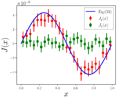
Figure 1: The average density current to $x$ and $y$-direction. Theoretical result Eq. (33) (Blue solid line) and the simulation result of the current for $x$-direction $J_{x}(x)$ (Red dots) and $y$-direction $J_{y}(x)$ are shown. The error bar for the simulation result is the standard error. The parameters are $\alpha=0.2,T^{*}=0.002,B^{*}=0.1$.

Since we have truncated the expansion up to the linear order in $\omega_{\mathrm{s}}$, we chose a relatively small value of $B^{*}$.

Next, we investigate the $B$-dependence of the current. The current has the sinusoidal profile fitted by $A\sin(2\pi x)$ and we plot the $B$ dependence of the amplitude $A$ in Figure 2 together with the theoretical prediction. The theoretical prediction is $A={16\pi^{3}\alpha N^{(0)}T^{*}B^{*}}/{9\gamma^{4}}$ from Eq. (33).

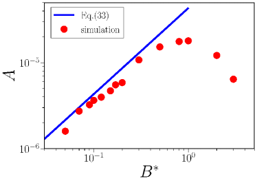
Figure 2: The $B$-dependence of the current intensity for the theoretical result (Blue solid line) and the simulation result (Red dots). Simulation parameters are $\alpha=0.2,T^{*}=0.002$.

In the small $B$-regime, the simulation result agrees well with the theoretical prediction. As $B$ increases, the simulation result reaches a peak and then decreases. Note that the magnetic field for which the cyclotron frequency becomes comparable with the inverse of the velocity relaxation time, $\omega_{s}\tau=1$, is at $B^{\ast}\approx 1$. The value agrees with the position of the peak of $A$ shown in Fig. 2. This implies that when the magnetic field is strong, the cyclotron frequency is very fast and the cyclotron radius becomes small, which reduces the bend of the particle trajectories, as is the case for the Nernst coefficient for the rarefied gases [17]. This nonlinear effect is not taken into account in our theoretical analysis (Eq. (33)) because we retain only the linear terms in $B$.

IV semi-quantitative argument

We provide a semi-quantitative argument about how the anomalous transport arises and why the current depends on $\partial_{x}^{3}T$. Let us consider the hydrodynamic description of the Brownian particles. In the stationary state, the frictional force due to the current and the osmotic pressure should be balanced. If the magnetic field is present, the Lorentz force should be also added, so that we have

$$0=-\nabla p-\zeta\bm{J}-q\bm{B}\times\bm{J},$$ (36)

where $p$ is the osmotic pressure field and $\bm{J}$ is the velocity field (and not the velocity of respective particles). Inverting the equation, we obtain the solution for $J_{y}$ given by

$$J_{y}(x)\approx-\frac{\omega_{s}\tau}{\zeta}\frac{\partial p}{\partial x}$$ (37)

up to the linear order in $B$. For the non-interacting Brownian particles, the osmotic pressure is given by $p=\rho k_{\mathrm{B}}T$. This is exact if the local equilibrium condition is satisfied. We assume that $p$ is still proportional to $\rho T$ even when the local equilibrium condition is violated. We expand $\rho$ as $\rho(x)=\rho^{(0)}(x)+\rho^{(1)}(x)+\cdots$ in the $1/\gamma$-expansion. As we have shown in Section II (see Eq. (22)), $\rho^{(0)}(x)T(x)=$constant for the lowest order term in the steady state in the case that the conserved force is absent. This solution corresponds to the overdamped approximation [15]. The next order terms in $1/\gamma$ is $\rho^{(2)}$ ($=c_{0,0}^{(2)}$ in Section II) . $\rho^{(2)}$ satisfies

$$\begin{split}\left(\frac{\partial}{\partial x}+\frac{2}{v_{\mathrm{th}}}\frac{\partial v_{\mathrm{th}}}{\partial x}\right)\rho^{(2)}=-\sqrt{2}\left(\frac{\partial}{\partial x}+\frac{2}{v_{\mathrm{th}}}\frac{\partial v_{\mathrm{th}}}{\partial x}\right)c^{(2)}_{2,0}.\end{split}$$ (38)

We have already derived $c^{(2)}_{2,0}$ in Section II (see Eq. (28)). The solution of this equation is

$$\rho^{(2)}=-\frac{N^{(0)}}{2T(x)\gamma^{2}}\frac{\partial^{2}T(x)}{\partial x^{2}}+\frac{mN^{(0)}}{k_{\mathrm{B}}T(x)}N^{(2)}.$$ (39)

where $N^{(0)}$ is a normalization constant for $c^{(0)}_{0,0}$ introduced at Eq. (32) and $N^{(2)}=\sqrt{2}\int c^{(2)}_{2,0}dx$ is a normalization constant which is determined in such a way that $\int\rho^{(2)}dx=0$. It is noteworthy that Eq. (39) does not depend on $B$ and is present in the absence of $B$. Combining the above results, we conclude that the osmotic pressure gradient is not zero but instead it is given by

$$\begin{split}\frac{\partial p}{\partial x}&=\frac{\partial}{\partial x}\rho^{(2)}(x)k_{\mathrm{B}}T(x)=-\frac{k_{\mathrm{B}}N^{(0)}}{2\gamma^{2}}\frac{\partial^{3}T(x)}{\partial x^{3}}.\end{split}$$ (40)

Combining this expression with Eq. (37), we arrive at

$$\begin{split}J_{y}(x)=\frac{\omega_{s}N^{(0)}}{2\gamma^{4}}\frac{\partial^{3}}{\partial x^{3}}\frac{k_{\mathrm{B}}T(x)}{m}\\ \end{split}$$ (41)

Aside from a numerical factor, this is identical to our final result, Eq. (33). We conclude that the small deviation of the density field from the local equilibrium induces the local pressure modulation, $\partial p/\partial x\neq 0$ which causes the local velocity field in the $x$-direction and eventually leads to the velocity field in the $y$-direction. The current in the $x$-direction is only local and net current integrated over $x$-direction should vanish.

V Discussion and Conclusions

We have shown that there exists a stationary density current of non-interacting Brownian particles perpendicular to the temperature modulation and the magnetic field, even when the system is confined in the direction of the temperature modulation by the wall or the periodic boundary condition. This Nernst-like effect is proportional to the magnetic field and the third derivative of the temperature modulation. This has been explained by analytically solving the Kramers equation by the standard inverse friction expansion. These effects are beyond the linear response regime in that the current is due to the super Burnett correction or the higher-order derivative of the temperature gradient. This anomalous current can not be explained in the overdamped limit, which corresponds to the lowest order contribution in the $1/\gamma$ expansion, at which the local equilibrium assumption is valid.

It is not easy practically to observe the anomalous current in realistic systems because the large magnetic field and the small friction coefficient are required. However, it is important to recognize that the coupling between the force which does not satisfy the time-reversal symmetry can induce the macroscopic current, if small, in the simple classical system. In active matter systems, the non-conserved force which violates the time-reversal symmetry combined with the strong nonequilibrium conditions is ubiquitous [27, 28, 7, 8, 9, 29, 30]. The coupling of the effect of the inertia and the nonequilibrium conditions is also known to bring about the nontrivial macroscopic effect in active matter systems, in stark contrast with the equilibrium Brownian motion where the short time scales are relevant in the underdamped equation does not affect the macroscopic behaviors [31, 32]. The result in this paper demonstrates the counter-intuitive effects due to a subtle interplay between the non-conserved force (the Lorentz force), the nonequilibrium condition (the inhomogeneous temperature), and the inertia effect (the finite $m$) in possibly the simplest model system. Considering the coupling of these effects in realizable systems such as active matter systems is a promising future direction.