On Faster Convergence of Scaled Sign Gradient Descent

Abstract

Communication has been seen as a significant bottleneck in industrial applications over large-scale networks. To alleviate the communication burden, sign-based optimization algorithms have gained popularity recently in both industrial and academic communities, which is shown to be closely related to adaptive gradient methods, such as Adam. Along this line, this paper investigates faster convergence for a variant of sign-based gradient descent, called scaled SIGNGD, in three cases: 1) the objective function is strongly convex; 2) the objective function is nonconvex but satisfies the Polyak-Łojasiewicz (PL) inequality; 3) the gradient is stochastic, called scaled SIGNSGD in this case. For the first two cases, it can be shown that the scaled SIGNGD converges at a linear rate. For case 3), the algorithm is shown to converge linearly to a neighborhood of the optimal value when a constant learning rate is employed, and the algorithm converges at a rate of $O(1/k)$ when using a diminishing learning rate, where $k$ is the iteration number. The results are also extended to the distributed setting by majority vote in a parameter-server framework. Finally, numerical experiments on logistic regression are performed to corroborate the theoretical findings.

I Introduction

This paper studies an unconstrained optimization problem

$$\min_{x\in\mathbb{R}^{d}}f(x),$$ (1)

where the objective $f:\mathbb{R}^{d}\to\mathbb{R}$ is a proper differentiable function, and may be nonconvex, which has numerous applications in industry, such as electric vehicles [1, 2], smart grid [3], internet of things (IoT) [4], and so on. To solve this problem, a quintessential algorithm is the gradient descent (GD) method [5, 6, 7], which requires to access true gradients. However, it is usually expensive or difficult to compute the true gradients in reality, and thereby a typical stochastic gradient descent (SGD) algorithm has become prevalent in deep neural networks [8, 9], which depends upon a lower computing cost for stochastic gradients.

As for large-scale neural networks, the training efficiency can be substantially improved in general by introducing multiple workers in a parameter-server framework, where a group of workers can train their own mini-batch datasets in parallel. Nonetheless, the communication between workers and the parameter server has been a non-negligible handicap for its wide practical application. As such, as one of gradient compression techniques, sign-based methods have been popular in recent decades, not only because they can reduce the communication cost to one bit for each gradient coordinate, but because they have good performance and close relationship with adaptive gradient methods [10, 11, 12]. As a matter of fact, it has been demonstrated in [13, 11] that SIGNSGD with momentum often has pretty similar performance to Adam on deep learning missions in practice. Notice that a wide range of gradient compression approaches exist for reducing the communication cost in the literature, e.g., [14, 15], whose elaboration is beyond the scope of this paper. Particularly, sign-based methods considered in this paper can be regarded as a special gradient compression scheme which need to transmit only one bit per gradient component [16].

Along this line, the sign gradient descent (SIGNGD) algorithm and its stochastic counterpart (SIGNSGD) have been extensively studied in recent years [17, 11, 18, 12, 19], which are, respectively, of the form

$$x_{k+1} =x_{k}-\alpha_{k}\operatorname{sign}(\nabla f(x_{k})),$$ (2)

$$x_{k+1} =x_{k}-\alpha_{k}\operatorname{sign}(h_{k}),$$ (3)

where $h_{k}\in\mathbb{R}^{d}$ is a stochastic gradient of $f$ at $x_{k}$, $\alpha_{k}>0$ is the learning rate, and the signum function $\operatorname{sign}$ is operated componentwise. For instance, it was demonstrated in [11] that SIGNSGD enjoys a SGD-level convergence rate for nonconvex but smooth objective functions under a separable smoothness assumption, which, in combination with majority vote in distributed setup, was further shown to be efficient in terms of communication and fault toleration in [18]. Recently, the authors in [12] found that the $\ell_{\infty}$-smoothness is a weaker and natural assumption than the separable smoothness and established two conditions under which the sign-based methods are preferable over GD.

Contributions. To our best knowledge, this paper is the first to address faster convergence of sign methods with more details as follows.

First, it is found that SIGNGD is not generally convergent even for strongly convex and smooth objectives when using constant learning rates, although it is indeed convergent for vanilla GD. Therefore, scaled versions in Algorithms 1 and 2 are investigated. It is proved that Algorithm 1 converges linearly to the minimal value for two cases: strongly convex objectives and nonconvex objectives yet satisfying the Polyak-Łojasiewicz (PL) inequality. Meanwhile, Algorithm 2 converges linearly to a neighborhood of the minimal value when using a constant learning rate $\alpha$ with an error being proportional to $\alpha^{2}$ and the variance of stochastic gradients. When applying a kind of diminishing learning rate, a rate $O(\ln^{2}(k)/k^{2})$ can be ensured for (15), which is superior to the widely known rate $O(1/k)$ [20].

Second, the obtained results are extended to the distributed setup, where a group of workers compute their own (stochastic) gradients using individual dataset and then transmit the sign gradient and the gradient $\ell_{1}$-norm to the parameter server who calculates the sign gradient by majority vote along with taking the average of the gradient $\ell_{1}$-norms and transmits back to all the workers.

Notations. Denote by $[n]:=\{1,2,\ldots,n\}$ for an integer $n>0$. Let $\|\cdot\|$, $\|\cdot\|_{1}$, $\|\cdot\|_{\infty}$ and $x^{\top}$ be the $\ell_{2}$-norm, $\ell_{1}$-norm, $\ell_{\infty}$-norm and the transpose of $x\in\mathbb{R}^{n}$, respectively. $\mathbf{1}$ and $\mathbf{0}$ stand for column vectors of compatible dimension with all entries being $1$ and $0$, respectively. $\nabla f$ represents the gradient of a function $f$. $\mathbb{E}(\cdot)$ and $\mathbb{P}(\cdot)$ denote the mathematical expectation and probability, respectively.

II Counterexamples for SIGNGD

For SIGNGD, an interesting result can also be found in the continuous-time setup, which demonstrates obvious advantages of SIGNGD compared with GD. Particularly, SIGNGD converges linearly, while GD is only sublinearly convergent. More details are postponed to the Appendix as supplemental materials.

Motivated by the fact in the continuous-time setup, it seems promising to consider the discrete-time counterpart of (23), i.e., SIGNGD (2) with $\alpha_{k}=\alpha>0$ being a constant learning rate. However, it is not the case. It is well known that GD is linearly convergent for small enough $\alpha>0$, while several counterexamples are presented below for illustrating that the sign counterpart (2) is generally not convergent even for strongly convex and smooth objectives.

Example 1.

Consider $f(x)=x_{1}^{2}+x_{2}^{2}$ for $x\in\mathbb{R}^{2}$, which is strongly convex and smooth with $\nabla f(x)=(2x_{1},2x_{2})^{\top}$. By choosing the initial point as $x_{0}=(\alpha/2,\alpha/2)^{\top}$, it is easy to verify for (2) that for $l=0,1,2,\ldots$,

$$x_{2l}=\big{(}-\frac{\alpha}{2},-\frac{\alpha}{2}\big{)}^{\top},~{}~{}~{}x_{2l+1}=\big{(}\frac{\alpha}{2},\frac{\alpha}{2}\big{)}^{\top},$$ (4)

which is obviously not convergent.

Example 1 shows that the exact convergence cannot be ensured for SIGNGD even for strongly convex and smooth objectives. To fix it, one may attempt to consider the sign counterpart of adaptive gradient methods. However, it generally does not work as well. For instance, the AdaGrad-Norm [21]

$$b_{k+1}^{2} =b_{k}^{2}+\|\nabla f(x_{k})\|^{2},$$

$$x_{k+1} =x_{k}-\frac{\eta}{b_{k+1}}\nabla f(x_{k}),~{}~{}~{}\eta>0$$ (5)

is shown to converge linearly without knowing any function parameters beforehand [22], while the linear convergence cannot be ensured in general for its sign counterparts, as illustrated below for its two sign variants.

Example 2.

Consider the first sign variant as

$$b_{k+1}^{2} =b_{k}^{2}+\|\nabla f(x_{k})\|^{2},$$

$$x_{k+1} =x_{k}-\frac{\eta}{b_{k+1}}\operatorname{sign}(\nabla f(x_{k})),~{}~{}~{}\eta>0$$ (6)

and $f(x)=x^{2}/2$ (strongly convex and smooth) with $x\in\mathbb{R}$. For simplicity, set $b_{0}=0$ and $x_{0}\neq 0$. Then simple manipulations give rise to $b_{k+1}^{2}=\sum_{l=0}^{k}x_{l}^{2}$.

In what follows, we show that the convergence rate of (6) is not linear. To do so, it is easy to see that $x_{k+1}=x_{k}-\frac{\eta}{b_{k+1}}\operatorname{sign}(x_{k})$, which leads to that

$$x_{k+1}^{2} =x_{k}^{2}-\frac{2\eta}{b_{k+1}}|x_{k}|+\frac{\eta^{2}}{b_{k+1}^{2}}$$

$$=x_{k}^{2}-\frac{\eta}{b_{k+1}^{2}}(2b_{k+1}|x_{k}|-\eta).$$ (7)

By contradiction, if $x_{k}$ or $f(x_{k})$ is linearly convergent, then one has that $\sum_{k=0}^{\infty}x_{k}^{2}\leq B$ for some constant $B>0$, which, together with (7) and $b_{k+1}^{2}=\sum_{l=0}^{k}x_{l}^{2}$, gives

$$x_{k+1}^{2}\geq x_{k}^{2}-\frac{\eta}{b_{k+1}^{2}}(2\sqrt{B}|x_{k}|-\eta).$$ (8)

After $|x_{k}|$ decreases to where $|x_{k}|\leq\frac{\eta}{2\sqrt{B}}$, invoking (8) leads to $x_{k+1}^{2}\geq x_{k}^{2}$, thus implying that $f(x_{k})$ will finally oscillate around the origin, which is a contradiction with the linear convergence of $f(x_{k})$. Hence, (6) is not linearly convergent.

Example 3.

Consider now another sign variant as

$$b_{k+1}^{2} =b_{k}^{2}+\|\operatorname{sign}(\nabla f(x_{k}))\|^{2},$$

$$x_{k+1} =x_{k}-\frac{\eta}{b_{k+1}}\operatorname{sign}(\nabla f(x_{k})),~{}~{}~{}\eta>0$$ (9)

and let $f=x^{2}$ (strongly convex and smooth) with $x\in\mathbb{R}$ with initial $x_{0}=\eta/2$ and $b_{0}=0$. In this case, it is straightforward to calculate that $b_{k}=\sqrt{k}$ and

$$x_{k} =\eta\Big{(}\frac{1}{2}-1+\frac{1}{\sqrt{2}}-\frac{1}{\sqrt{3}}+\cdots+\frac{(-1)^{k}}{\sqrt{k}}\Big{)},$$ (10)

from which one can conclude that (6) amounts to

$$x_{k+1}=x_{k}-\frac{\eta}{\sqrt{k+1}}\operatorname{sign}(x_{k}),$$ (11)

which can be viewed as GD for the convex objective $g(x)=|x|$ with a learning rate $\eta/\sqrt{k+1}$. Therefore, the convergence rate of classic GD can be invoked for (8), which is known to be sublinear [23].

Remark 1.

The above examples demonstrate that although GD and AdaGrad-Norm are indeed linearly convergent for strongly convex and smooth objectives, their sign counterparts fail to converge linearly in general.

III Linear Rate of Scaled SIGNGD/SGD

With the above preparations, it is now ready to study faster convergence for solving problem (1). As shown in Section II, the sign counterparts of GD and AdaGrad-Norm are not applicable for linear convergence. As such, the scaled versions of SIGNGD/SGD are considered in this paper, as in Algorithms 1 and 2, which can be viewed as the steepest descent with respect to the maximum norm [12], but is still not fully understood.

A few assumptions are necessary for the following analysis.

Assumption 1.

$f$ is $\mu$-strongly convex with respect to $\ell_{\infty}$-norm for some constant $\mu>0$, i.e., $f(x)-f(y)\geq\nabla f(y)^{\top}(x-y)+\frac{\mu}{2}\|x-y\|_{\infty}^{2}$ for all $x,y\in\mathbb{R}^{d}$.

Assumption 2.

$f$ satisfies the Polyak-Łojasiewicz (PL) inequality, i.e., $\|\nabla f(x)\|_{1}^{2}\geq 2\mu(f(x)-f^{*}),~{}\forall x\in\mathbb{R}^{d}$, where $f^{*}$ is the minimum value.

Assumption 3.

$f$ is $L$-smooth with respect to $\ell_{\infty}$-norm, i.e., $\|\nabla f(x)-\nabla f(y)\|_{1}\leq L\|x-y\|_{\infty}$ for all $x,y\in\mathbb{R}^{d}$.

The PL inequality does not require $f$ to be even convex, and the $\ell_{\infty}$- and $\ell_{1}$-norms employed in Assumptions 1 and 2, respectively, are slightly more relaxed than the Euclidean norm. Meanwhile, the smoothness condition is made with respect to $\ell_{\infty}$-norm, since it is more favorable than the Euclidean smoothness and separable smoothness [12].

Remark 2.

It is noteworthy that another promising sign method is EF-SIGNGD [16] using error feedback, given as

$$p_{k} =\lambda\nabla f(x_{k})+e_{k},$$

$$x_{k+1} =x_{k}-\frac{\|p_{k}\|_{1}}{d}\operatorname{sign}(p_{k}),$$

$$e_{k+1} =p_{k}-\frac{\|p_{k}\|_{1}}{d}\operatorname{sign}(p_{k}),$$ (12)

where $\lambda>0$ is the learning rate. In [16], it is shown that EF-SIGNGD/SGD has a better performance than SIGNGD/SGD, actually enjoying the same convergence rate as GD/SGD. However, we point out that EF-SIGNGD/SGD is, roughly speaking, equivalent to GD/SGD. Let us show this by slightly modifying (12) as

$$p_{k} =\lambda\nabla f(x_{k}-e_{k})+e_{k},$$

$$x_{k+1} =x_{k}-\frac{\|p_{k}\|_{1}}{d}\operatorname{sign}(p_{k}),$$

$$e_{k+1} =p_{k}-\frac{\|p_{k}\|_{1}}{d}\operatorname{sign}(p_{k}).$$ (13)

By defining $z_{k}=x_{k}-e_{k}$, it is easy to verify that $z_{k+1}=z_{k}-\lambda\nabla f(z_{k})$, that is, (13) amounts to GD in terms of $z_{k}$. As a result, EF-SIGNGD/SGD is not considered here.

In the following, the main results are divided into two scenarios, i.e., the deterministic and stochastic settings.

Algorithm 1 Scaled SIGNGD

  Input: learning rate $\alpha$, current point $x_{k}$

  

$$x_{k+1}=x_{k}-\alpha\|g_{k}\|_{1}\operatorname{sign}(g_{k}),~{}~{}~{}g_{k}:=\nabla f(x_{k})$$ (14)

Algorithm 2 Scaled SIGNSGD

  Input: learning rate $\alpha_{k}$, current point $x_{k}$

  

$$\tilde{g}_{k}=\text{StochasticGradient}(x_{k})$$

$$x_{k+1}=x_{k}-\alpha_{k}\|\tilde{g}_{k}\|_{1}\operatorname{sign}(\tilde{g}_{k})$$ (15)

III-A The Deterministic Setting

Consider the deterministic setting with full gradients, i.e., (14), for which we have the following results. Note that all proofs are given in the Appendix.

Theorem 1.

The following statements are true for (14).

1. Under Assumptions 1 and 3, if $0<\alpha<\frac{2}{L}$, then

   $$f(x_{k})-f^{*}\leq\zeta^{k}(f(x_{0})-f^{*}),$$ (16)

   where $\zeta:=1-2\mu\alpha\big{(}1-\frac{L\alpha}{2}\big{)}\in[0,1)$.

2. Under Assumptions 2 and 3 with $\alpha$ satisfying $0<\alpha<\frac{2}{L}$, (16) still holds.

3. If Assumption 3 holds only, then

   $$\min_{l\in\{0,1,\ldots,k\}}\|g_{l}\|_{1}^{2}\leq\frac{f(x_{0})-f^{*}}{\gamma(k+1)},$$ (17)

   where $\gamma:=\alpha(1-\frac{L\alpha}{2})$.

Remark 3.

In view of Theorem 1, the algorithm (14) is proved to be linearly convergent, which is contrast to SIGNGD and sign AdaGrad-Norm as discussed in Section II. Moreover, for the nonconvex but smooth with respect to the Euclidean norm, by leveraging the similar argument to Theorem 1, it is easy to obtain for SIGNGD with a constant learning rate that $\min_{l\in\{0,1,\ldots,k\}}\|g_{l}\|_{1}^{2}\leq\frac{dL(f(x_{0})-f^{*})}{2(k+1)}$ by choosing the learning rate as $\alpha=\sqrt{\frac{2(f(x_{0})-f^{*})}{dL(k+1)}}$. In comparison, (17) can be nearly $\frac{L(f(x_{0})-f^{*})}{2(k+1)}$ when $\alpha$ is chosen to approach $\frac{2}{L}$. In this regard, our result is tighter up to a dimension constant $d$, and the learning rate here is easier to implement. In addition, if the smoothness is with respect to the maximum norm, then the result here has the same convergence bound as SIGNGD but with a less conservative learning rate selection.

Remark 4.

A similar result can be also obtained from the most related work [24] by resorting to the $\delta$-approximate compressor. To be specific, $\mathcal{C}(v):=\frac{\|v\|_{1}}{d}\operatorname{sign}(v)$ can be viewed as $\frac{1}{d}$-approximate compressor, and then applying Theorem 13 in [24] leads to the learning rate $\alpha\in[0,\frac{1}{L}]$ and convergence rate $(1-\frac{\alpha\mu}{d})^{k}$. In contrast, Theorem 1 of this paper (need to replace $\alpha$ by $\frac{\alpha}{d}$ here) is for $\alpha\in(0,\frac{2d}{L})$ with the convergence rate $(1-\frac{2\mu\alpha}{d}(1-\frac{L\alpha}{2}))^{k}$. It is easy to verify that our learning rate is more relaxed and the convergence rate is faster due to $\frac{\alpha\mu}{d}\leq\frac{2\mu\alpha}{d}(1-\frac{L\alpha}{2})$.

III-B The Stochastic Setting

This section considers the stochastic gradient case, where the true gradient $g_{k}=\nabla f(x_{k})$ is expensive to compute and instead a stochastic gradient $\tilde{g}_{k}$ is relatively cheap to evaluate as an estimate of $g_{k}$. To move forward, some standard assumptions are imposed on stochastic gradients [13, 11].

Assumption 4.

The stochastic gradients $\{\tilde{g}_{k}\}_{k=0}^{\infty}$ are unbiased and have bounded variances with respect to $\ell_{1}$-norm, i.e., there exists a constant $\sigma>0$ such that

$$\mathbb{E}(\tilde{g}_{k})=g_{k},~{}~{}~{}~{}~{}\mathbb{E}(\|\tilde{g}_{k}-g_{k}\|_{1}^{2})\leq\sigma^{2}.$$ (18)

In this case, the algorithm becomes (15). For brevity, define $p_{k,i}:=\mathbb{P}(\operatorname{sign}(\tilde{g}_{k,i})=\operatorname{sign}(g_{k,i}))$ for $k\geq 0$ and $i\in[d]$, where $\tilde{g}_{k,i}$ and $g_{k,i}$ represents the $i$-th components of $\tilde{g}_{k,i}$ and $g_{k}$, respectively.

Remark 5.

For stochastic gradient $g_{k}$, when leveraging a mini-batch of size $n_{k}$ at $x_{k}$, the oracle gives us $n_{k}$ gradient estimates and in this case, the stochastic gradient $\tilde{g}_{k}$ can be chosen as the average of $n_{k}$ estimates. In this respect, the variance bound can be reduced to $\frac{\sigma^{2}}{n_{k}}$. Additionally, it was shown in [19] that the success probability $p_{k,i}$ should be greater than $1/2$, and otherwise the sign algorithm generally fails to work. And a multitude of cases can ensure $p_{k,i}>1/2$, for instance, each component $\tilde{g}_{k,i}$ possesses a unimodal and symmetric distribution [11, 19].

We are now in a position to present the main result on (15).

Theorem 2.

For (15), under Assumptions 1, 3, 4 or 2-4, the following statements are true.

1. If $\alpha_{k}=\alpha\in\big{(}0,\frac{2p_{min}-1}{L}\big{)}$, then

   $$\mathbb{E}(f(x_{k}))-f^{*} \leq\zeta_{1}^{k}(\mathbb{E}(f(x_{0}))-f^{*})$$

   $$\hskip 11.38092pt+\frac{L\sigma^{2}\alpha}{2\mu(2p_{min}-1-L\alpha)},$$ (19)

   where $p_{min}:=\min_{i\in[d],k\geq 0}p_{k,i}$ and $\zeta_{1}:=1-2\mu\alpha(2p_{min}-1-L\alpha)\in[\frac{1}{2},1)$.

2. If $\alpha_{k}=\frac{3}{\mu(2p_{min}-1)(k+1)}$, then

   $$\mathbb{E}(f(x_{k}))-f^{*} \leq\frac{9L\sigma^{2}}{\mu^{2}(2p_{min}-1)^{2}}\Big{(}\frac{32}{k}+\frac{1}{k^{2}}\Big{)}$$

   $$\hskip 11.38092pt+\frac{f(x_{0})-f^{*}}{(k+1)^{3}}.$$ (20)

Remark 6.

The first result in Theorem 2 shows that algorithm (15) converges linearly at a rate $\zeta_{1}$. This is comparable to vanilla SGD in [25], where the convergence rate is $1-\alpha\mu$, which is slower than $\zeta_{1}$ (i.e., $\zeta_{1}\leq 1-\alpha\mu$) when $\alpha\in(0,\frac{1}{2L})$. Moreover, the result in (20) is the exact convergence with rate $O(\frac{1}{k})$ for both strongly convex case and nonconvex case with PL inequality, which is the same as both vanilla SGD [26] and compression methods [20]. In addition, the same rate $O(\frac{1}{k})$ was established in [27]. However, the condition in [27] for convergence does not always hold, e.g., $t_{k}=1$ in Theorem II.2 of [27], and our result (20) includes more faster rate $O(\frac{1}{k^{2}}+\frac{1}{k^{3}})$ except for $O(\frac{1}{k})$ in [27].

IV The Distributed Setting

Now, we extend the results in Section III to the distributed setting within a parameter server framework. For simplicity, we only focuses on scaled SIGNSGD in this section, but the results can be similarly obtained for scaled SIGNGD.

Algorithm 3 Distributed Scaled SIGNSGD by Majority Vote

  Input: learning rate $\alpha$, current point $x_{k}$, $\#$ workers $M$ each with an i.i.d. gradient estimate $\tilde{g}_{k}^{m},m\in[M]$

  On server        Pull $\operatorname{sign}(\tilde{g}_{k}^{m})$ and $\|\tilde{g}_{k}^{m}\|_{1}$ from each worker       Push $\operatorname{sign}(\hat{g}_{k}^{s})$ and $M_{k}$ to each worker               $\hat{g}_{k}^{s}:=\frac{1}{M}\sum_{m=1}^{M}\operatorname{sign}(\tilde{g}_{k}^{m})$               $M_{k}:=\frac{1}{M}\sum_{m=1}^{M}\|\tilde{g}_{k}^{m}\|_{1}$

  On each worker        $x_{k+1}=x_{k}-\alpha M_{k}\operatorname{sign}(\hat{g}_{k}^{s})$

To proceed, the distributed scaled SIGNSGD by majority vote is given in Algorithm 3, for which the following convergence result is obtained.

Theorem 3.

For Algorithm 3, under Assumptions 1, 3, 4 or 2-4, if $0<\alpha<\frac{2I_{p_{min}}(\kappa,\kappa)-1}{L}$, then

$$\mathbb{E}(f(x_{k}))-f^{*}\leq\zeta_{2}^{k}(\mathbb{E}(f(x_{0}))-f^{*})+\frac{L\sigma^{2}\alpha^{2}}{1-\zeta_{2}},$$ (21)

where $p_{min}=\min_{l\in[d],k\geq 0}p_{k,l}$, $\zeta_{2}:=1-2\mu\alpha(2I_{p_{min}}(\kappa,\kappa)-1-L\alpha)\in[\frac{1}{2},1)$, $\kappa:=\lfloor\frac{M+1}{2}\rfloor$ with $\lfloor\cdot\rfloor$ being the floor function, and $I_{p}(a,b)$ is the regularized incomplete beta function, defined by

$$I_{p}(a,b):=\frac{\int_{0}^{p}t^{a-1}(1-t)^{b-1}dt}{\int_{0}^{1}t^{a-1}(1-t)^{b-1}dt},~{}~{}~{}a,b>0,~{}p\in[0,1].$$

Remark 7.

It is noteworthy that the exact convergence can be similarly established as (20) in Theorem 2, which is omitted in Theorem 3.

V Experiments

Numerical experiments are provided to corroborate the efficacy of the obtained theoretical results here.

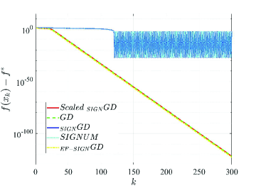
Figure 1: Simulation results for several algorithms.

Example 4 (A Toy Example).

Let us consider a simple example, where $f(x)=x^{2}+3\sin^{2}(x)$ for $x\in\mathbb{R}$. It is easy to verify that $f(x)$ is nonconvex, but satisfying the PL condition. To verify the performance of the proposed scaled SIGNGD, several existing algorithms are compared in Fig. 1 by setting $\alpha=0.05$ with an arbitrary initial state. The comparisons are performed with vanilla gradient descent (GD), SIGNGD, SIGNGDM (i.e., SIGNUM), and EF-SIGNGD [16]. It can be observed from Fig. 1 that the proposed algorithm has the same linear convergence as GD and EF-SIGNGD, while SIGNGD and SIGNUM cannot converge, behaving oscillations near the optimal variable. In summary, this example shows the efficiency of the scaled SIGNGD, and supports the observation in Example 1.

Example 5.

Consider the logistic regression problem, where the objective is $f(x)=\frac{1}{n}\sum_{i=1}^{n}\log(1+\exp(-b_{i}a_{i}^{\top}x))+\frac{1}{2n}\|x\|^{2}$ with a standard $L2$-regularizer [20], and $a_{i}\in\mathbb{R}^{d}$ and $b_{i}\in\{-1,+1\}$ are the data samples.

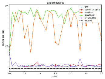
Figure 2: Scaled SIGNSGD. (a) $\alpha=2$; (b) $\alpha_{k}=\frac{6n}{k+1}$.

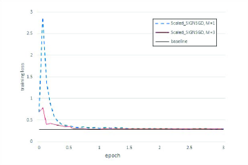
Figure 3: Distributed scaled SIGNSGD for $M=1,3$.

To test the performance of scaled SIGNSGD, the epsilon dataset with $n=400000$ and $d=2000$ is exploited [28], and the baseline is calculated using the standard optimizer LogisticSGD of scikit-learn [29]. To marginalize out the effect of initial choices, the numerical result is averaged over repeated runs with $x_{0}\approx\mathcal{N}(0,I)$. We compare scaled SIGNSGD with vanilla SGD, SIGNSGD, SIGNSGDM, and EF-SIGNSGD [16], as shown in Fig. 2 on a platform with the Intel Core i7-4300U CPU. Fig. 2 indicates that SIGNSGD has a similar performance to SGD and performs better than SIGNSGD and SIGNSGDM. It can be also observed that EF-SIGNSGD is comparable to SGD, which is consistent with the discussion in Remark 2. Moreover, the case in Fig. 2(a) with a constant learning rate converges faster than that in Fig. 2(b) with a diminishing learning rate. Meanwhile, Fig. 3 shows that more workers can improve the performance. Therefore, the numerical results support our theoretical findings.

VI Conclusion

This paper has investigated faster convergence of scaled SIGNGD/SGD, which can relieve the communication cost compared with vanilla SGD. To further motivate the study of sign methods, continuous-time algorithms have been addressed, indicating that sign SGD can significantly improve the convergence speed of SGD. Subsequently, it has been proven that scaled SIGNGD is linearly convergent for both strongly convex and nonconvex (satisfying PL inequality) objectives. Also, the convergence for SIGNSGD has been analyzed in two cases with constant and decaying learning rates. The results are also extended to the distributed setting in the parameter server framework. The efficacy of scaled sign methods has been validated by numerical experiments for the logistic regression problem.

Appendix

VI-A Further Motivations for SIGNGD

Let us provide more evidences for studying sign-based GD from the continuous-time perspective. In doing so, consider the continuous-time dynamics corresponding to the discrete-time GD and SIGNGD, i.e.,

$$\dot{x} =-\beta\nabla f(x),$$ (22)

$$\dot{x} =-\beta\operatorname{sign}(\nabla f(x)),$$ (23)

where $\beta>0$ is a constant learning rate.

To proceed, let us construct a Lyapunov candidate as

$$V(t):=f(x)-f^{*},~{}~{}~{}\forall~{}t\geq 0$$ (24)

where $f^{*}$ denotes the minimum value attained by $f$.

For algorithms (22) and (23), the following results can be obtained.

Proposition 1.

For algorithm (22),

1. if $f$ is convex, then $V(t)\leq\frac{D_{1}^{2}V(0)}{D_{1}^{2}+V(0)\beta t}$, where $D_{1}:=\max_{x:f(x)\leq f(x_{0})}\min_{x^{*}\in\mathcal{X}^{*}}\|x-x^{*}\|$ with $\mathcal{X}^{*}$ being the set of minimizers;

2. if $f$ is nonconvex, then $\min_{s\in[0,t]}\|\nabla f(x(s))\|\leq\frac{\sqrt{f(x(0))-f^{*}}}{\sqrt{\beta t}}$.

Proposition 2.

For algorithm (23),

1. if $f$ is convex, then $V(t)\leq V(0)e^{-\frac{\beta t}{D_{2}}}$, where $D_{2}:=\max_{x:f(x)\leq f(x_{0})}\min_{x^{*}\in\mathcal{X}^{*}}\|x-x^{*}\|_{\infty}$;

2. if $f$ is nonconvex, then $\min_{s\in[0,t]}\|\nabla f(x(s))\|_{1}\leq\frac{f(x(0))-f^{*}}{\beta t}$.

In view of the above results, it can be easily observed that (23) with sign gradients converges apparently faster than GD (22) in the continuous-time domain, indicating that the performance of gradient descent can be largely improved by sign gradient compression. For instance, in the scenario with convex objectives, GD (22) is sublinearly convergent while SIGNGD (23) is linearly convergent. As a result, the above results provide a new perspective for showing advantages of SIGNGD compared with GD.

VI-B Proof of Proposition 1

Consider the case with convex objectives. In light of (22), it can be calculated that

$$\dot{V}(t)=\nabla f(x(t))^{\top}\dot{x}=-\beta\|\nabla f(x(t))\|^{2}\leq 0,$$ (25)

which implies $f(x(t))\leq f(x(0))$.

Meanwhile, invoking the convexity of $f$ yields

$$V(t) \leq\nabla f(x(t))^{\top}(x-x^{*})$$

$$\leq\|\nabla f(x(t))\|\cdot\|x-x^{*}\|$$

$$\leq D_{1}\|\nabla f(x(t))\|,$$ (26)

which, together with (25), gives rise to $\dot{V}(t)\leq-\frac{\beta}{D_{1}^{2}}V(t)^{2}$, further implying the claimed result.

For the case with nonconvex objectives, by integrating (25) from $0$ to $t$, one can obtain that

$$\beta\int_{0}^{t}\|\nabla f(x(s))\|^{2}ds =V(0)-V(t)$$

$$=f(x(0))-f(x(t))$$

$$\leq f(x(0))-f^{*},$$ (27)

where the inequality has employed the fact that $f(z)\geq f^{*}$ for all $z\in\mathbb{R}^{d}$. Then taking the minimum of $\|\nabla f(x(s))\|$ over $[0,t]$ ends the proof. ∎

VI-C Proof of Proposition 2

Consider first the convex case. Similar to (25), it can be obtained that

$$\dot{V}(t)=-\beta\|\nabla f(x(t))\|_{1}.$$ (28)

Akin to (26), one has that

$$V(t) \leq\nabla f(x(t))^{\top}(x-x^{*})$$

$$\leq\|\nabla f(x(t))\|_{1}\cdot\|x-x^{*}\|_{\infty}$$

$$\leq D_{2}\|\nabla f(x(t))\|_{1},$$ (29)

where the second inequality has used Holder’s inequality. Combining (28) with (29) yields $\dot{V}(t)\leq-\frac{\beta}{D_{2}}V(t)$, from which it is easy to verify the claimed result.

Consider now the nonconvex case. The desired result can be obtained by (28) and the similar argument to that in convex case. This completes the proof. ∎

VI-D Proof of Theorem 1

To facilitate the subsequent analysis, define

$$V_{k}:=f(x_{k})-f^{*},~{}~{}~{}\forall k\geq 0.$$ (30)

In view of (14) and Assumption 3, it can be concluded that

$$V_{k+1}-V_{k} =f(x_{k+1})-f(x_{k})$$

$$\leq\nabla f(x_{k})^{\top}(x_{k+1}-x_{k})+\frac{L}{2}\|x_{k+1}-x_{k}\|_{\infty}^{2}$$

$$=-\alpha\|g_{k}\|_{1}^{2}+\frac{L\alpha^{2}}{2}\|g_{k}\|_{1}^{2}\cdot\|\operatorname{sign}(g_{k})\|_{\infty}^{2}$$

$$\leq-\alpha\|g_{k}\|_{1}^{2}+\frac{L\alpha^{2}}{2}\|g_{k}\|_{1}^{2}$$

$$=-\gamma\|g_{k}\|_{1}^{2}.$$ (31)

In what follows, let us prove this theorem one by one.

First, for case 1, invoking Assumption 1 yields

$$V_{k} \leq g_{k}^{\top}(x_{k}-x^{*})-\frac{\mu}{2}\|x_{k}-x^{*}\|_{\infty}^{2}$$

$$\leq\frac{1}{2}\Big{(}\frac{\|g_{k}\|_{1}^{2}}{\mu}+\mu\|x_{k}-x^{*}\|_{\infty}^{2}\Big{)}-\frac{\mu}{2}\|x_{k}-x^{*}\|_{\infty}^{2}$$

$$=\frac{\|g_{k}\|_{1}^{2}}{2\mu},$$

where the second inequality has employed the Holder inequality. Then one has that $\|g_{k}\|_{1}^{2}\geq 2\mu V_{k}$. Therefore, in combination with (31), one can obtain that $V_{k+1}-V_{k}\leq-2\mu\gamma V_{k}$, further leading to $V_{k+1}\leq\zeta V_{k}$. Consequently, by iteration, this completes the proof of case 1.

Second, for case 2, Assumption 2 leads to $2\mu V_{k}\leq\|g_{k}\|_{1}^{2}$, which, together with the similar argument to case 1, follows the conclusion in this case.

Third, for case 3, invoking (31) gives $\gamma\|g_{k}\|_{1}^{2}\leq V_{k}-V_{k+1}$, which, by summation over $l=0,1,\ldots,k$, implies that

$$\gamma\sum_{l=0}^{k}\|g_{l}\|_{1}^{2} \leq V_{0}-V_{k+1}=f(x_{0})-f(x_{k+1})$$

$$\leq f(x_{0})-f^{*},$$ (32)

where the last inequality has used the fact that $f(x_{k+1})\geq f^{*}$. Then taking the minimum of $\|g_{l}\|_{1}^{2}$ over $l=0,1,\ldots,k$ ends the proof. ∎

VI-E Proof of Theorem 2

Recalling $V_{k}$ in (30). Invoking Assumption 3 gives rise to

$$V_{k+1}-V_{k} \leq g_{k}^{\top}(x_{k+1}-x_{k})+\frac{L}{2}\|x_{k+1}-x_{k}\|_{\infty}^{2}$$

$$=-\alpha\|\tilde{g}_{k}\|_{1}g_{k}^{\top}\operatorname{sign}(\tilde{g}_{k})+\frac{L\alpha^{2}}{2}\|\tilde{g}_{k}\|_{1}^{2}\|\operatorname{sign}(\tilde{g}_{k})\|_{\infty}^{2}$$

$$\leq-\alpha\|\tilde{g}_{k}\|_{1}g_{k}^{\top}\operatorname{sign}(\tilde{g}_{k})+\frac{L\alpha^{2}}{2}\|\tilde{g}_{k}\|_{1}^{2}.$$

By taking the conditional expectation, one has

$$\mathbb{E}(V_{k+1}|x_{k})-V_{k} \leq-\alpha g_{k}^{\top}\mathbb{E}(\|\tilde{g}_{k}\|_{1}\operatorname{sign}(\tilde{g}_{k})|x_{k})$$

$$\hskip 11.38092pt+\frac{L\alpha^{2}}{2}\mathbb{E}(\|\tilde{g}_{k}\|_{1}^{2}|x_{k}).$$ (33)

Consider now the coordinate $\tilde{g}_{k,i}$ for $i\in[d]$. One has that

$$\mathbb{E}(\|\tilde{g}_{k}\|_{1}\operatorname{sign}(\tilde{g}_{k,i})|x_{k}) =\mathbb{E}[\mathbb{E}(\|\tilde{g}_{k}\|_{1}\operatorname{sign}(\tilde{g}_{k,i})|\tilde{g}_{k})|x_{k}]$$

$$=\mathbb{E}[\|\tilde{g}_{k}\|_{1}\mathbb{E}(\operatorname{sign}(\tilde{g}_{k,i})|\tilde{g}_{k})|x_{k}]$$

$$=\mathbb{E}[\|\tilde{g}_{k}\|_{1}\mathbb{P}(\operatorname{sign}(\tilde{g}_{k,i})=\operatorname{sign}(g_{k,i}))\operatorname{sign}(g_{k,i})$$

$$-\|\tilde{g}_{k}\|_{1}\mathbb{P}(\operatorname{sign}(\tilde{g}_{k,i})\neq\operatorname{sign}(g_{k,i}))\operatorname{sign}(g_{k,i})|x_{k}]$$

$$=\mathbb{E}[p_{k,i}\|\tilde{g}_{k}\|_{1}\operatorname{sign}(g_{k,i})-(1-p_{k,i})\|\tilde{g}_{k}\|_{1}\operatorname{sign}(g_{k,i})|x_{k}]$$

$$=(2p_{k,i}-1)\operatorname{sign}(g_{k,i})\mathbb{E}(\|\tilde{g}_{k}\|_{1}|x_{k}),$$

which, together with (33), implies that

$$\mathbb{E}(V_{k+1}|x_{k})-V_{k} \leq-\alpha\sum_{i=1}^{d}(2p_{k,i}-1)|g_{k,i}|\mathbb{E}(\|\tilde{g}_{k}\|_{1}|x_{k})$$

$$\hskip 11.38092pt+\frac{L\alpha^{2}}{2}\mathbb{E}(\|\tilde{g}_{k}\|_{1}^{2}|x_{k}).$$ (34)

By Jesen’s inequality, it follows that $\mathbb{E}(\|\tilde{g}_{k}\|_{1}|x_{k})\geq\|\mathbb{E}(\tilde{g}_{k}|x_{k})\|_{1}=\|g_{k}\|_{1}$. Because $p_{k,i}\geq p_{min}$ for $i\in[d]$, taking the expectation implies that

$$\mathbb{E}(V_{k+1})-\mathbb{E}(V_{k}) \leq-\alpha(2p_{min}-1)\mathbb{E}(\|g_{k}\|_{1}^{2})$$

$$+L\alpha^{2}[\mathbb{E}(\|\tilde{g}_{k}-g_{k}\|_{1}^{2})+\mathbb{E}(\|g_{k}\|^{2})]$$

$$\leq-\alpha(2p_{min}-1-L\alpha)\mathbb{E}(\|g_{k}\|_{1}^{2})+L\sigma^{2}\alpha^{2}.$$ (35)

Now, under Assumption 1 or 2, using the similar argument to the proof of Theorem 1 can both lead to that $\mathbb{E}(\|g_{k}\|_{1}^{2})\geq 2\mu\mathbb{E}(V_{k})$, which together with (35) yields that

$$\mathbb{E}(V_{k+1})\leq\zeta_{1}\mathbb{E}(V_{k})+L\sigma^{2}\alpha^{2}.$$ (36)

Iteratively applying the above inequality leads to (19).

It remains to show (20). Invoking the similar analysis for (36) yields that

$$\mathbb{E}(V_{k+1})\leq c_{k}\mathbb{E}(V_{k})+L\sigma^{2}\alpha_{k}^{2},$$

where $c_{k}:=1-\alpha_{k}\mu(2p_{min}-1)$, further implying that

$$\mathbb{E}(V_{k}) \leq\Pi_{l=0}^{k-1}c_{l}V_{0}+L\sigma^{2}(c_{k-1}\cdots c_{1}\alpha_{0}^{2}+\cdots$$

$$\hskip 11.38092pt+c_{k-1}\alpha_{k-2}^{2}+\alpha_{k-1}^{2})$$

$$\leq\Pi_{l=0}^{k-1}c_{l}V_{0}+\frac{9}{\mu^{2}(2p_{min}-1)^{2}}$$

$$\hskip 42.67912pt\cdot\Big{(}\sum_{m=1}^{k-1}e^{-\sum_{l=m}^{k-1}\frac{3}{l+1}}\frac{1}{m^{2}}+\frac{1}{k^{2}}\Big{)},$$ (37)

where the second inequality has employed the expression of $\alpha_{k}$.

For the last two terms in (37), in light of the fact that $\Pi_{l=0}^{m}(1-a_{l})\leq e^{-\sum_{l=0}^{m}a_{l}}$ for $a_{l}\in[0,1]$, one has that

$$\Pi_{l=0}^{k-1}c_{l} \leq e^{-\mu(2p_{min}-1)\sum_{l=0}^{k-1}\alpha_{l}}$$

$$\leq\frac{1}{(k+1)^{3}},$$ (38)

and

$$\sum_{m=1}^{k-1}e^{-\sum_{l=m}^{k-1}\frac{3}{l+1}}\frac{1}{m^{2}} \leq\sum_{m=1}^{k-1}\frac{(m+1)^{3}}{(k+1)^{3}}\frac{1}{m^{2}}$$

$$\leq\sum_{m=1}^{k-1}\frac{8m^{3}}{(k+1)^{3}m^{2}}$$

$$\leq\frac{4}{k}.$$ (39)

Then inserting (38) and (39) to (37) leads to the conclusion (20). The proof is complete. ∎

VI-F Proof of Theorem 3

To ease the exposition, define $\hat{g}_{k}:=\{\tilde{g}_{k}^{m},m\in[M]\}$. Invoking Assumptions 3 and Algorithm 3 yields

$$V_{k+1}-V_{k}\leq-\alpha M_{k}g_{k}^{\top}\operatorname{sign}(\hat{g}_{k}^{s})+\frac{L\alpha^{2}}{2}M_{k}^{2},$$

which, by taking the conditional expectation, implies that

$$\mathbb{E}(V_{k+1}|x_{k})-V_{k} \leq-\alpha g_{k}^{\top}\mathbb{E}(M_{k}\operatorname{sign}(\hat{g}_{k}^{s})|x_{k})$$

$$\hskip 11.38092pt+\frac{L\alpha^{2}}{2}\mathbb{E}(M_{k}^{2}|x_{k}).$$ (40)

For $g_{k}^{\top}\mathbb{E}(M_{k}\operatorname{sign}(\hat{g}_{k}^{s})|x_{k})$ in (40), one has

$$g_{k}^{\top}\mathbb{E}(M_{k}\operatorname{sign}(\hat{g}_{k}^{s})|x_{k}) =g_{k}^{\top}\mathbb{E}(M_{k}\mathbb{E}(\operatorname{sign}(\hat{g}_{k}^{s})|\hat{g}_{k})|x_{k})$$

$$=\mathbb{E}(M_{k}\sum_{i=1}^{d}g_{k,i}\mathbb{E}(\operatorname{sign}(\hat{g}_{k,i}^{s})|\hat{g}_{k})|x_{k})$$

$$=\mathbb{E}(M_{k}\sum_{i=1}^{d}|g_{k,i}|\mathbb{E}(\operatorname{sign}(\hat{g}_{k,i}^{s}g_{k,i})|\hat{g}_{k})|x_{k})$$

$$=\mathbb{E}(M_{k}\sum_{i=1}^{d}|g_{k,i}|(2I_{p_{k,i}}(\kappa,\kappa)-1)|x_{k})$$

$$\geq(2I_{p_{min}}(\kappa,\kappa)-1)\|g_{k}\|_{1}\mathbb{E}(M_{k}|x_{k}),$$ (41)

where the last equality has exploited Lemma 7 in [19], and the inequality comes from the fact that $p_{k,i}\geq p_{min}$ for $i\in[d],k\geq 0$.

As for the last term in (41), it can be concluded that

$$\mathbb{E}(M_{k}|x_{k}) \geq\mathbb{E}(\big{\|}\frac{1}{M}\sum_{m=1}^{M}\tilde{g}_{k}^{m}\big{\|}_{1}|x_{k})$$

$$\geq\big{\|}\mathbb{E}(\frac{1}{M}\sum_{m=1}^{M}\tilde{g}_{k}^{m}|x_{k})\big{\|}_{1}$$

$$=\|g_{k}\|_{1},$$

which, combining with (40) and (41), leads to

$$\mathbb{E}(V_{k+1})-\mathbb{E}(V_{k}) \leq-\alpha(2I_{p_{min}}(\kappa,\kappa)-1)\mathbb{E}(\|g_{k}\|_{1}^{2})$$

$$\hskip 11.38092pt+\frac{L\alpha^{2}}{2}\mathbb{E}(M_{k}^{2}).$$ (42)

Now, for the last term in (42), one has

$$\mathbb{E}(M_{k}^{2}) \leq\frac{1}{M}\sum_{m=1}^{M}\mathbb{E}(\|\tilde{g}_{k}^{m}\|_{1}^{2})$$

$$\leq\frac{2}{M}\sum_{m=1}^{M}\mathbb{E}(\|\tilde{g}_{k}^{m}-g_{k}\|_{1}^{2})+2\mathbb{E}(\|g_{k}\|_{1}^{2})$$

$$\leq 2\sigma^{2}+2\mathbb{E}(\|g_{k}\|_{1}^{2}),$$

which, together with (42), yields

$$\mathbb{E}(V_{k+1})-\mathbb{E}(V_{k})$$

$$\hskip 11.38092pt\leq-\alpha(2I_{p_{min}}(\kappa,\kappa)-1-L\alpha)\mathbb{E}(\|g_{k}\|_{1}^{2})+L\sigma^{2}\alpha^{2}.$$

The rest of proof is similar to that after (35). This ends the proof. ∎

References

• [1] J. Shen, S. Dusmez, and A. Khaligh, “Optimization of sizing and battery cycle life in battery/ultracapacitor hybrid energy storage systems for electric vehicle applications,” IEEE Transactions on Industrial Informatics, vol. 10, no. 4, pp. 2112–2121, 2014.
• [2] X. Li, X. Yi, and L. Xie, “Distributed online optimization for multi-agent networks with coupled inequality constraints,” IEEE Transactions on Automatic Control, in press, doi: 10.1109/TAC.2020.3021011, 2020.
• [3] W. Su, H. Eichi, W. Zeng, and M.-Y. Chow, “A survey on the electrification of transportation in a smart grid environment,” IEEE Transactions on Industrial Informatics, vol. 8, no. 1, pp. 1–10, 2011.
• [4] S. Messaoud, A. Bradai, and E. Moulay, “Online GMM clustering and mini-batch gradient descent based optimization for industrial IoT 4.0,” IEEE Transactions on Industrial Informatics, vol. 16, no. 2, pp. 1427–1435, 2019.
• [5] S. Ruder, “An overview of gradient descent optimization algorithms,” arXiv preprint arXiv:1609.04747, 2016.
• [6] M. Meng and X. Li, “Aug-PDG: Linear convergence of convex optimization with inequality constraints,” arXiv preprint arXiv:2011.08569, 2020.
• [7] X. Li, L. Xie, and Y. Hong, “Distributed aggregative optimization over multi-agent networks,” IEEE Transactions on Automatic Control, in press, DOI: 10.1109/TAC.2021.3095456, 2021.
• [8] L. Bottou, “Stochastic gradient descent tricks,” in Neural Networks: Tricks of the Trade.   Springer, 2012, pp. 421–436.
• [9] S. Bonnabel, “Stochastic gradient descent on Riemannian manifolds,” IEEE Transactions on Automatic Control, vol. 58, no. 9, pp. 2217–2229, 2013.
• [10] M. Riedmiller and H. Braun, “A direct adaptive method for faster backpropagation learning: The RPROP algorithm,” in International Conference on Neural Networks, San Francisco, USA, 1993, pp. 586–591.
• [11] J. Bernstein, Y.-X. Wang, K. Azizzadenesheli, and A. Anandkumar, “signSGD: Compressed optimisation for non-convex problems,” in International Conference on Machine Learning, Stockholm, Sweden, 2018, pp. 560–569.
• [12] L. Balles, F. Pedregosa, and N. L. Roux, “The geometry of sign gradient descent,” arXiv preprint arXiv:2002.08056, 2020.
• [13] L. Balles and P. Hennig, “Dissecting Adam: The sign, magnitude and variance of stochastic gradients,” in International Conference on Machine Learning, Stockholm, Sweden, 2018, pp. 404–413.
• [14] J. Hamer, M. Mohri, and A. T. Suresh, “FedBoost: A communication-efficient algorithm for federated learning,” in International Conference on Machine Learning, 2020, pp. 3973–3983.
• [15] C. Xie, S. Zheng, O. O. Koyejo, I. Gupta, M. Li, and H. Lin, “CSER: Communication-efficient SGD with error reset,” in Advances in Neural Information Processing Systems, vol. 33, 2020.
• [16] S. P. Karimireddy, Q. Rebjock, S. Stich, and M. Jaggi, “Error feedback fixes signSGD and other gradient compression schemes,” in International Conference on Machine Learning, 2019, pp. 3252–3261.
• [17] F. Seide, H. Fu, J. Droppo, G. Li, and D. Yu, “1-bit stochastic gradient descent and its application to data-parallel distributed training of speech DNNs,” in Fifteenth Annual Conference of the International Speech Communication Association, Singapore, 2014, pp. 1058–1062.
• [18] J. Bernstein, J. Zhao, K. Azizzadenesheli, and A. Anandkumar, “signSGD with majority vote is communication efficient and fault tolerant,” in International Conference on Learning Representations, 2019.
• [19] M. Safaryan and P. Richtárik, “On stochastic sign descent methods,” arXiv preprint arXiv:1905.12938, 2019.
• [20] S. U. Stich, J.-B. Cordonnier, and M. Jaggi, “Sparsified SGD with memory,” in Advances in Neural Information Processing Systems, Montréal, Canada, 2018, pp. 4447–4458.
• [21] R. Ward, X. Wu, and L. Bottou, “AdaGrad stepsizes: Sharp convergence over nonconvex landscapes,” in International Conference on Machine Learning, 2019, pp. 6677–6686.
• [22] Y. Xie, X. Wu, and R. Ward, “Linear convergence of adaptive stochastic gradient descent,” in International Conference on Artificial Intelligence and Statistics, Palermo, Italy, 2020, pp. 1475–1485.
• [23] A. Nedić and A. Olshevsky, “Distributed optimization over time-varying directed graphs,” IEEE Transactions on Automatic Control, vol. 60, no. 3, pp. 601–615, 2015.
• [24] A. Beznosikov, S. Horváth, P. Richtárik, and M. Safaryan, “On biased compression for distributed learning,” arXiv preprint arXiv:2002.12410, 2020.
• [25] R. M. Gower, N. Loizou, X. Qian, A. Sailanbayev, E. Shulgin, and P. Richtárik, “SGD: General analysis and improved rates,” in International Conference on Machine Learning, Long Beach, California, 2019, pp. 5200–5209.
• [26] A. Rakhlin, O. Shamir, and K. Sridharan, “Making gradient descent optimal for strongly convex stochastic optimization,” in International Conference on Machine Learning, Edinburgh, Scotland, UK, 2012, pp. 1571–1578.
• [27] D. Carlson, Y.-P. Hsieh, E. Collins, L. Carin, and V. Cevher, “Stochastic spectral descent for discrete graphical models,” IEEE Journal of Selected Topics in Signal Processing, vol. 10, no. 2, pp. 296–311, 2015.
• [28] S. Sonnenburg, V. Franc, E. Yom-Tov, and M. Sebag, “Pascal large scale learning challenge,” vol. 10, pp. 1937–1953, 2008.
• [29] F. Pedregosa, G. Varoquaux, A. Gramfort, V. Michel, B. Thirion, O. Grisel, M. Blondel, P. Prettenhofer, R. Weiss, V. Dubourg et al., “Scikit-learn: Machine learning in Python,” Journal of Machine Learning Research, vol. 12, pp. 2825–2830, 2011.