Generalized local ansatz for scale-dependent primordial non-Gaussianities and future galaxy surveys

Abstract

We revisit a possible scale-dependence of local-type primordial non-Gaussianities induced by super-horizon evolution of scalar field perturbations. We develop the formulation based on $\delta N$ formalism and derive the generalized form of the local-type bispectrum and also trispectrum which allows us to implement the scale-dependence and suitably compare model prediction with observational data. We propose simple but phenomenologically meaningful expressions, which encompass the information of a wide range of physically motivated models. We also formulate large-scale power spectrum and bispectrum of biased objects in the presence of the scale-dependent primordial non-Gaussianities. We perform the Fisher analysis for future galaxy surveys and give the projected constraints on the parameters of the generalized local-form of primordial non-Gaussianities.

1 Introduction

In the standard cosmology, the primordial fluctuations are assumed to be described by a Gaussian distribution, and characterized by an almost scale-invariant power spectrum. However, possible small deviations from a purely Gaussian primordial density fluctuations, called primordial non-Gaussianity, have also been extensively investigated. Since the primordial non-Gaussianity reflects the fundamental interactions and nonlinear processes involved during and after the inflation, it can bring insights into the generation mechanism of primordial density fluctuations. Among several types of primordial non-Gaussianities, the local-type one has been studied widely. In the simplest case, the curvature perturbation $\zeta$ can be expanded in terms of the purely Gaussian variable $\zeta_{\rm g}$ as (Komatsu and Spergel, 2001)

$$\zeta=\zeta_{\rm g}+\frac{3}{5}f_{\rm NL}\zeta_{\rm g}^{2}+\frac{9}{25}g_{\rm NL}\zeta_{\rm g}^{3}+\cdots\,,$$ (1)

which leads to the bispectrum and the trispectrum of the following form:

$$B_{\zeta}(k_{1},k_{2},k_{3})=\frac{6}{5}f_{\rm NL}\Bigl{[}P_{\zeta}(k_{1})P_{\zeta}(k_{2})+{\rm 2\ perms}\Bigr{]}\,,$$ (2)

$$T_{\zeta}(k_{1}k_{2},k_{3},k_{4})=\tau_{\rm NL}\Bigl{[}P_{\zeta}(k_{1})P_{\zeta}(k_{2})P_{\zeta}(k_{13})+{\rm 11\ perms}\Bigr{]}$$

$$\quad\quad\quad\quad\quad\quad\quad\quad+\frac{54}{25}g_{\rm NL}\Bigl{[}P_{\zeta}(k_{1})P_{\zeta}(k_{2})P_{\zeta}(k_{3})+{\rm 3\ perms}\Bigr{]}~{}.$$ (3)

Here $f_{\rm NL},~{}g_{\rm NL},$ and $\tau_{\rm NL}$ are called nonlinearity parameters for the local-type and usually assumed to be constant. $P_{\zeta}(k)$ denotes the power spectrum of the curvature perturbations, and $k_{13}=|{\bf k}_{1}+{\bf k}_{3}|$. The generation of the local-type primordial non-Gaussianity through the super-horizon evolution can be evaluated by using the $\delta N$ formalism (Starobinsky, 1986; Salopek and Bond, 1990; Sasaki and Stewart, 1995; Sasaki and Tanaka, 1998; Lyth, Malik, and Sasaki, 2004; Lyth and Rodriguez, 2005). We consider $\delta N$ with an initial flat hypersurface at $t_{\rm i}$, on which the initial values of the fields have a certain distribution, and follow its evolution until reaching the final uniform energy density hypersurface at $t_{\rm f}$. The $\delta N$ formalism gives the curvature perturbations contributed generally from the multiple scalar fields $\phi^{I}(t,{\bf x})$ which are calculated through the perturbation of the $e$-folding number measured between the initial and the final surfaces:

$$\zeta(t_{\rm f},{\bf x})=\delta N(t_{\rm f},\phi^{I}(t_{\rm i},{\bf x}))\,.$$ (4)

Based on the above formula, expanding in terms of the field perturbations, we can systematically calculate the bispectrum and trispectrum of the primordial curvature perturbations and evaluate the nonlinearity parameters $f_{\rm NL}$, $\tau_{\rm NL}$ and $g_{\rm NL}$.

The nonlinearity parameters have primarily been constrained from the higher-order spectrum in cosmic microwave background (CMB) (see (Akrami et al., 2018) for recent constraints from Planck). However, the current CMB measurements are already reaching to the precision of the cosmic-variance limited one. A complementary way to access primordial non-Gaussianity is to measure the spatial clustering behavior of halos/galaxies on large scales. One of the most distinctive effect of the local-type primordial non-Gaussianity is the enhancement of the large-scale clustering of biased objects, which is due to the non-linear coupling generated by the primordial non-Gaussianity (Dalal et al., 2008; Desjacques, Seljak, and Iliev, 2209). In fact, it has been shown that the power spectrum measurements of galaxy clustering in future surveys such as Square Kilometre Array Observatory (SKAO)  in radio wavelengths (see e.g., (Bacon et al., 2020; Yamauchi et al., 2016)) and Euclid  in optical and infrared bands can constrain the nonlinearity parameters to the level comparable to or tighter than CMB measurements (see e.g. (Ferramacho et al., 2014; Yamauchi, Takahashi, and Oguri, 2014; de Putter and Doré, 2014; Yamauchi and Takahashi, 2015)). So far, the cosmological analysis of large-scale structure surveys has relied on matter and galaxy power spectrum, however the extra information can also be extracted with higher-order correlation functions, namely matter and galaxy bispectrum, which is expected to have a great potential to drastically improve the constraints on not only the primordial non-Gaussianity (Jeong and Komatsu, 2009; Hashimoto et al., 2016; Tellerini et al., 2016; Yamauchi, Yokoyama, and Takahashi, 2016; Shirasaki et al., 2021) but also modified theories of gravity (Yamauchi, Yokoyama, and Tashiro, 2017; Yamauchi and Sugiyama, 2021).

In this paper, we revisit the extension of the simplest model of the local-type non-Gaussianity with implementing the scale-dependence of the nonlinearity parameters. Although in many literatures the local-type nonlinearity parameters are frequently assumed to be scale-independent as in Eq. (1), there are several possible sources that generate a scale-dependent primordial non-Gaussianity. For instance, in models with multiple scalar fields where a field other than the inflaton can be responsible for the curvature perturbation (see, e.g., (Suyama et al., 2010) for various models and their predictions for non-Gaussianities), the non-linear evolution after the horizon exit can generate scale-dependent local-type non-Gaussianities (see e.g.,  (Yokoyama, Suyama, and Tanaka, 2007a, b; Byrnes et al., 2010a, b; Byrnes and Gong, 2012) for a general discussion on scale-dependence of non-Gaussianities, see (Byrnes, Enqvist, and Takahashi, 2010; Huang, 2010a, b; Byrnes et al., 2011; Huang and Lin, 2011; Kobayashi and Takahashi, 2012; Byrnes and Tarrant, 2015) for some explicit models). On the observational side, there have been several works which obtain constraints on the scale-dependence of non-Gaussianities from CMB (Becker and Huterer, 2012; Oppizzi et al., 2018) and large scale structure (Dai and Xia, 2020). Some works investigate expected constraints from future galaxy surveys (Raccanelli, Dore, and Dalal, 2014; Ballardini, Mattherson, and Maartens, 2019) (see also (Sefusatti et al., 2009; Giannantonio et al., 2012; Becker, Huterer, and Kadota, 2012; Biagetti et al., 2013) for the pre-Planck analysis). Actually, the galaxy power spectrum analysis alone may not accurately constrain the scale-dependence of the primordial non-Gaussianity. Hence, we expect that the combination of the galaxy power and bi-spectra provides us with the unique opportunity to probe the scale-dependence of the primordial non-Gaussianity to some accuracy. In the light of this, we revisit the scale-dependence of the nonlinearity parameters which arise in some realistic inflationary models and explore the impact of the use of both the galaxy power and bi-spectra in future large-scale structure surveys.

This paper is organized as follows. In Sec. 2 we revisit the $\delta N$ formalism to evaluate the scale-dependence of primordial bi- and tri-spectra. In particular, we derive the generalized form of the local-type primordial non-Gaussianities at leading order in slow-roll expansion for the scale dependence. Based on the derived expression, we then calculate the galaxy power- and bi-spectrum, and show the generalized form of the scale-dependent biases in Sec. 3. In Sec. 4 we quantitatively estimate the impact of the generalized local-type primordial non-Gaussianities and the use of the galaxy bispectrum to probe primordial non-Gaussianities in SKAO and Euclid as future representative large-scale structure surveys. Finally, Sec. 5 is devoted to the summary and discussion.

2 Generalized local form of primordial non-Gaussianities

In this section, we discuss the scale-dependence of the local-type primordial non-Gaussianities generated on super-horizon scales, based on the $\delta N$ formalism. We consider the multiple scalar fields which can contribute to a scale-dependence of the nonlinearity parameters. As shown below, there are two ways to generate the scale-dependence. The first one is due to the different scale-dependence of the various Gaussian fields. The second one is the evolution of perturbations after horizon exit. Following Refs. (Yokoyama, Suyama, and Tanaka, 2007a, b; Byrnes et al., 2010a, b), we will show the explicit form of the scale-dependence of nonlinearity parameters $f_{\rm NL},\tau_{\rm NL}$ and $g_{\rm NL}$, in which both of these types are properly incorporated.

2.1 General argument

We start with the Lagrangian governing the system, which is given by

$${\cal L}=-\frac{1}{2}g^{\mu\nu}\delta_{IJ}\partial_{\mu}\phi^{I}\partial_{\nu}\phi^{J}-V(\phi^{K})\,.$$ (5)

For simplicity, we assume a flat metric in field space. Based on $\delta N$ formalism (Starobinsky, 1986; Salopek and Bond, 1990; Sasaki and Stewart, 1995; Sasaki and Tanaka, 1998; Lyth, Malik, and Sasaki, 2004; Lyth and Rodriguez, 2005), we expand the Fourier components of the curvature perturbation on super-horizon scales in terms of the fluctuations of the scalar fields as

$$\zeta(t_{\rm f},{\bf k})= N_{I}(t_{\rm f},t_{\rm i})\delta\phi^{I}(t_{\rm i},{\bf k})+\frac{1}{2}N_{IJ}(t_{\rm f},t_{\rm i})\left(\delta\phi^{I}\star\delta\phi^{J}\right)(t_{\rm i},{\bf k})$$ (6)

$$+\frac{1}{6}N_{IJK}(t_{\rm f},t_{\rm i})\left(\delta\phi^{I}\star\delta\phi^{J}\star\delta\phi^{K}\right)(t_{\rm i},{\bf k})+\cdots\,.$$

Here $(\delta\phi\star\delta\phi)$ and $(\delta\phi\star\delta\phi\star\delta\phi)$ denote the convolution defined as

$$\left(\delta\phi^{I}\star\delta\phi^{J}\right)(t_{\rm i},{\bf k}) :=\int\frac{\mathrm{d}^{3}{\bf p}}{(2\pi)^{3}}\delta\phi^{I}(t_{\rm i},{\bf p})\delta\phi^{J}(t_{\rm i},{\bf k}-{\bf p})\,,$$ (7)

$$\left(\delta\phi^{I}\star\delta\phi^{J}\star\delta\phi^{K}\right)(t_{\rm i},{\bf k}) :=\int\frac{\mathrm{d}^{3}{\bf p}}{(2\pi)^{3}}\int\frac{\mathrm{d}^{3}{\bf q}}{(2\pi)^{3}}\delta\phi^{I}(t_{\rm i},{\bf p})\delta\phi^{J}(t_{\rm i},{\bf q})\delta\phi^{K}(t_{\rm i},{\bf k}-{\bf p}-{\bf q})\,.$$ (8)

Here we take a uniform energy density (or comoving) slice at $t_{\rm f}$ and a spatially flat one at $t_{\rm i}$. The quantities $N(t_{\rm f},t_{\rm i})$, $N_{I}(t_{\rm f},t_{\rm i}):=\partial N(t_{\rm f},\phi^{K}(t_{\rm i}))/\partial\phi^{I}(t_{\rm i})$, $N_{IJ}(t_{\rm f},t_{\rm i}):=\partial^{2}N(t_{\rm f},\phi^{K}(t_{\rm i}))/\partial\phi^{I}(t_{\rm i})\partial\phi^{J}(t_{\rm i})$ and so on respectively denote the number of $e$-folds measured from $t_{\rm i}$ to $t_{\rm f}$, and their derivatives with respect to scalar fields at $t=t_{\rm i}$. In the framework of $\delta N$ formalism, the curvature perturbation depends on $t_{\rm f}$, but it should be independent on the choice of $t_{\rm i}$. However, the statistical property of the scalar field perturbations on the flat hypersurface at $t_{\rm i}$ would depend on the choice of $t_{i}$ due to their super-horizon non-linear growth. Thus, in usual, $t_{\rm i}$ is taken to be a certain time soon after the relevant length scale crossed the horizon scale, at when the scalar field perturbations on the flat hypersurface are supposed to be almost Gaussian in the slow-roll inflationary phase. Then the non-Gaussianities of the primordial curvature perturbation can be completely captured in the non-linear evolution of the number of $e$-folds measured from $t_{\rm i}$ to $t_{\rm f}$. In order to investigate the scale-dependence of the bi- and tri-spectra accurately, it is quite important to take the fact that the different momenta exit the horizon at different times, very carefully.

Now let us introduce $t_{\rm c}$ as the time at which all the scales of interest of the scalar field fluctuations have already exited the horizon though the slow-roll conditions for all the relevant scalar fields are still satisfied. As we have mentioned, the expression (6) is independent on the choice of $t_{\rm i}$, and hence $t_{\rm i}$ can be replaced with $t_{\rm c}$. In the replaced expression, $\delta\phi^{I}(t_{\rm c},{\bf k})$ is no longer the Gaussian due to the super-horizon non-linear growth. In order to evaluate the statistical property of $\delta\phi^{I}(t_{\rm c},{\bf k})$, we need to solve the evolution equations for scalar field perturbations and obtain the solution for $\delta\phi^{I}(t_{\rm c},{\bf k})$ order-by-order in terms of $\delta\phi^{I}(t_{\rm i},{\bf k})$ (see (Yokoyama, Suyama, and Tanaka, 2007a, b)). As far as we consider a mode which exits the horizon before $t=t_{\rm c}$, that is, $k<a(t_{\rm c})H(t_{\rm c})$, we can use the slow-roll approximation for solving the super-horizon evolution and in that approximation the slow-roll parameters are almost constant in time for $t_{\rm i}<t<t_{\rm c}$. Then, we can obtain the formal expressions as (Yokoyama, Suyama, and Tanaka, 2007a, b; Byrnes et al., 2010a, b)

$$\delta\phi^{I}(t_{\rm c},{\bf k})= \delta\phi_{(1)}^{I}(t_{\rm c},{\bf k})+\frac{1}{2}\delta\phi_{(2)}^{I}(t_{\rm c},{\bf k})+\frac{1}{6}\delta\phi_{(3)}^{I}(t_{\rm c},{\bf k})+\cdots\,,$$ (9)

with

$$\delta\phi_{(1)}^{I}(t_{\rm c},{\bf k})=\biggl{[}\delta^{I}{}_{J}+\epsilon^{I}{}_{J}\ln\left(\frac{a(t_{\rm c})H(t_{\rm c})}{a(t_{\rm i})H(t_{\rm i})}\right)\biggr{]}\delta\phi^{J}(t_{\rm i},{\bf k})\equiv\Lambda^{I}{}_{J}(t_{\rm c},t_{\rm i})\delta\phi^{J}(t_{\rm i},{\bf k})\,,$$ (10)

$$\delta\phi_{(2)}^{I}(t_{\rm c},{\bf k})=F^{I}_{(2)JK}\ln\left(\frac{a(t_{\rm c})H(t_{\rm c})}{a(t_{\rm i})H(t_{\rm i})}\right)\Bigl{(}\delta\phi_{(1)}^{J}\star\delta\phi_{(1)}^{K}\Bigr{)}(t_{\rm i},{\bf k})\,,$$ (11)

$$\delta\phi_{(3)}^{I}(t_{\rm c},{\bf k})=F^{I}_{(3)JKL}\ln\left(\frac{a(t_{\rm c})H(t_{\rm c})}{a(t_{\rm i})H(t_{\rm i})}\right)\Bigl{(}\delta\phi_{(1)}^{J}\star\delta\phi_{(1)}^{K}\star\delta\phi_{(1)}^{L}\Bigr{)}(t_{\rm i},{\bf k})\,.$$ (12)

Here, we have introduced the slow-roll suppressed coefficients $\epsilon^{I}{}_{J}$, $F^{I}_{(2)JK}$, $F^{I}_{(3)JKL}$, whose explicit expressions are presented in Appendix A. In order for Eqs. (10)–(12) to be valid, these parameters are constant in time from $t_{\rm i}$ to $t_{\rm c}$, and the logarithmic term should not grow very large. Indeed, when we consider observational scales where the scale-dependence of non-Gaussianities is probed, $\ln(a(t_{\rm c})H(t_{\rm c})/a(t_{\rm i})H(t_{\rm i}))={\cal O}(1)-{\cal O}(10)$, in which we can safely assume that slow-roll parameters are constant in time. Note that as shown in the above expression for each order, the non-linear relation between $\delta\phi^{I}(t_{\rm c})$ and $\delta\phi^{I}(t_{\rm i})$ are expressed at the leading order of $C_{\rm SR}\ln(a(t_{\rm c})H(t_{\rm c})/a(t_{\rm i})H(t_{\rm i}))$ with $C_{\rm SR}$ being the coefficient given by the combinations of slow-roll parameters such as $\epsilon^{I}_{J}$, $F^{I}_{(2)JK}$, and $F^{I}_{(3)JKL}$. As we will see later, this term gives the scale-dependence of the non-linearity parameters.

To evaluate the curvature perturbation, we choose the initial time $t_{\rm i}$ as that at the horizon crossing of a mode ${\bf k}$. Later, we will evaluate the bi- and tri-spectra of the curvature perturbations which are functions of the multiple wave numbers $\{{\bf k}_{i}\}$. For the different wave numbers, we need to consider the different horizon crossing times. Thus, hereinafter we denote the horizon crossing time of the mode $\bf k$ as $t_{\ast}(k)$ at which $a(t_{\ast}(k)H(t_{\ast}(k))=k$ holds and, in the following, we take $t_{\rm i}$ to be $t_{\ast}(k)$. Actually the convolution in Eq. (11) can be written as

$$\Bigl{(}\delta\phi_{(1)}^{I}\star\delta\phi_{(1)}^{J}\Bigr{)}(t_{\rm i},{\bf k})=\int\frac{\mathrm{d}^{3}{\bf p}}{(2\pi)^{3}}\delta\phi_{(1)}^{I}(t_{\rm i},{\bf p})\delta\phi_{(1)}^{J}(t_{\rm i},{\bf k}-{\bf p})\,.$$ (13)

(The similar expression holds for the convolution in Eq. (12).) Notice that $t_{\rm i}$ is not the horizon crossing time of the modes ${\bf p}$ nor ${\bf k}-{\bf p}$, and hence we need to specify the horizon crossing time for each mode separately.

Based on this formulation, $\delta\phi_{(1)}^{I}(t,{\bf k})$ can be treated as a Gaussian variable. Hence, by substituting Eqs. (9)–(12) into Eq. (6), we obtain the curvature perturbation evaluated at $t=t_{\rm c}$ rewritten in terms of the Gaussian variable $\delta\phi_{(1)}^{I}(t,{\bf k})$ as

$$\zeta(t_{\rm f},{\bf k})= N_{I}(t_{\rm f},t_{\rm c})\delta\phi^{I}(t_{\rm c},{\bf k})+\frac{1}{2}N_{IJ}(t_{\rm f},t_{\rm c})\left(\delta\phi^{I}\star\delta\phi^{J}\right)(t_{\rm c},{\bf k})$$

$$\quad\quad\quad\quad+\frac{1}{6}N_{IJK}(t_{\rm f},t_{\rm c})\left(\delta\phi^{I}\star\delta\phi^{J}\star\delta\phi^{K}\right)(t_{\rm c},{\bf k})+\cdots$$

$$= N_{I}^{\ast}(k)\delta\phi_{\ast}^{I}({\bf k})+\frac{1}{2}N_{IJ}^{\ast}(k)\Bigl{(}\delta\phi_{(1)}^{I}\star\delta\phi_{(1)}^{J}\Bigr{)}(t_{\ast}(k),{\bf k})$$ (14)

$$\quad\quad\quad\quad+\frac{1}{6}N_{IJK}^{\ast}(k)\Bigl{(}\delta\phi_{(1)}^{I}\star\delta\phi_{(1)}^{J}\star\delta\phi_{(1)}^{K}\Bigr{)}(t_{\ast}(k),{\bf k})+\cdots\,,$$

with (Byrnes et al., 2010b)

$$N_{I}^{\ast}(k)=N_{J}(t_{\rm f},t_{\rm c})\Lambda^{J}{}_{I}(t_{\rm c},t_{\ast}(k))\,,$$ (15)

$$N_{IJ}^{\ast}(k)=N_{I^{\prime}J^{\prime}}(t_{\rm f},t_{\rm c})\Lambda^{I^{\prime}}{}_{I}(t_{\rm c},t_{\ast}(k))\Lambda^{J^{\prime}}{}_{J}(t_{\rm c},t_{\ast}(k))$$

$$\quad\quad\quad\quad\quad+N_{K}(t_{\rm f},t_{\rm c})F^{K}_{(2)IJ}\ln\left(\frac{a(t_{\rm c})H(t_{\rm c})}{k}\right)\,,$$ (16)

$$N_{IJK}^{\ast}(k)=N_{I^{\prime}J^{\prime}K^{\prime}}(t_{\rm f},t_{\rm c})\Lambda^{I^{\prime}}{}_{I}(t_{\rm c},t_{\ast}(k))\Lambda^{J^{\prime}}{}_{J}(t_{\rm c},t_{\ast}(k))\Lambda^{K^{\prime}}{}_{K}(t_{\rm c},t_{\ast}(k))$$

$$\quad\quad\quad+\biggl{[}3N_{I^{\prime}L}(t_{\rm f},t_{\rm c})\Lambda^{I^{\prime}}{}_{I}(t_{\rm c},t_{\ast}(k))F^{L}_{(2)JK}+N_{L}(t_{\rm f},t_{\rm c})F^{L}_{(3)IJK}\biggr{]}\ln\left(\frac{a(t_{\rm c})H(t_{\rm c})}{k}\right)\,,$$ (17)

where for notational simplicity, we denote $\delta\phi_{\ast}^{I}({\bf k}):=\delta\phi^{I}(t_{\ast}(k),{\bf k})$.

Based on the derived expressions of the super-horizon evolution of the scalar-field perturbations, let us calculate the correlation functions of the curvature perturbation in Fourier space. The power spectrum of the scalar field perturbations during the slow-roll phase at the horizon crossing time is given by (see Ref. (Byrnes et al., 2010b))

$$\left\langle\delta\phi_{*}^{I}({\bf k})\delta\phi_{*}^{J}({\bf k}^{\prime})\right\rangle= (2\pi)^{3}\delta^{3}_{\rm D}({\bf k}+{\bf k})\frac{H^{2}(t_{*}(k))}{2k^{3}}\gamma^{IJ}\,,$$ (18)

where we have introduced $\gamma^{IJ}:=\delta^{IJ}-2\epsilon\delta^{I}{}_{J}+2(2-\ln 2-\gamma_{\rm E})\epsilon^{I}{}_{J}$ with $\epsilon=-\dot{H}/H^{2}$ and $\gamma_{\rm E}$ being the Euler-Mascheroni constant. By using this expression and Eq. (14), we obtain the power spectrum for the curvature perturbation defined by $\left\langle\zeta({\bf k})\zeta({\bf k}^{\prime})\right\rangle=(2\pi)^{3}\delta^{3}_{\rm D}({\bf k}+{\bf k}^{\prime})P_{\zeta}(k)$ in the form

$$P_{\zeta}(k)= \frac{H^{2}(t_{*}(k))}{2k^{3}}N^{\ast}_{I}(k)N_{\ast}^{I}(k)\,,$$ (19)

with $N_{\ast}^{I}(k):=N^{\ast}_{J}(k)\gamma^{IJ}$. Hereinafter, $t_{\rm f}$ in $\zeta$ is omitted. This immediately implies that the standard expression for the spectral index at the leading order as

$$n_{\rm s}-1:=\frac{\mathrm{d}\ln(k^{3}P_{\zeta}(k))}{\mathrm{d}\ln k}=-2\epsilon-2\frac{\epsilon^{IJ}N_{I}(t_{\rm f},t_{\rm c})N_{J}(t_{\rm f},t_{\rm c})}{N_{K}(t_{\rm f},t_{\rm c})N^{K}(t_{\rm f},t_{\rm c})}\,.$$ (20)

Actually, in this expression $\epsilon$ term comes from the derivative of $H$ and $\epsilon^{IJ}$ term can be obtained by the derivative of the linear propagator $\Lambda$ given in Eq. (10).

We now proceed to apply this approach to calculate the scale-dependence of the nonlinearity parameters. By making use of Eq. (14) and the fact that $\delta\phi_{(1)}^{I}(t,{\bf k})$ obeys the Gaussian statistics, the three-point function of the curvature perturbation in Fourier space is given by

$$\left\langle\zeta({\bf k}_{1})\zeta({\bf k}_{2})\zeta({\bf k}_{3})\right\rangle=N_{I}^{\ast}(k_{1})N_{J}^{\ast}(k_{2})N^{\ast}_{KL}(k_{3})$$

$$\quad\quad\times\int\frac{\mathrm{d}^{3}{\bf p}}{(2\pi)^{3}}\Big{\langle}\delta\phi_{\ast}^{I}({\bf k}_{1})\delta\phi_{(1)}^{K}(t_{\ast}(k_{3}),{\bf k}_{3}-{\bf p})\Big{\rangle}\Big{\langle}\delta\phi_{*}^{J}({\bf k}_{2})\delta\phi_{(1)}^{L}(t_{\ast}(k_{3}),{\bf p})\Big{\rangle}+(2~{}{\rm perms.})$$

$$\quad=(2\pi)^{3}\delta_{\rm D}^{3}({\bf k}_{1}+{\bf k}_{2}+{\bf k}_{3})N^{I}_{\ast}(k_{1})N^{J}_{\ast}(k_{2})N_{KL}^{\ast}(k_{3})$$

$$\quad\quad\times\Lambda^{K}{}_{I}(t_{\ast}(k_{3}),t_{\ast}(k_{1}))\Lambda^{L}{}_{J}(t_{\ast}(k_{3}),t_{\ast}(k_{2}))\frac{H^{2}(t_{*}(k_{1}))}{2k_{1}^{3}}\frac{H^{2}(t_{*}(k_{2}))}{2k_{2}^{3}}+(2~{}{\rm perms.})\,.$$ (21)

Defining the bispectrum as $\left\langle\zeta({\bf k}_{1})\zeta({\bf k}_{2})\zeta({\bf k}_{3})\right\rangle=(2\pi)^{3}\delta_{\rm D}^{3}({\bf k}_{1}+{\bf k}_{2}+{\bf k}_{3})B_{\zeta}(k_{1},k_{2},k_{3})$, and using (19), we obtain the expression for the generalized scale-dependent local form of the bispectrum for the curvature perturbation as (Byrnes et al., 2010b)

$$B_{\zeta}(k_{1},k_{2},k_{3})=\frac{6}{5}\widehat{f}_{\rm NL}(k_{1},k_{2},k_{3})P_{\zeta}(k_{1})P_{\zeta}(k_{2})+({\rm 2\ perms.})\,,$$ (22)

with

$$\frac{6}{5}\widehat{f}_{\rm NL}(k_{1},k_{2},k_{3})= \frac{N^{I}_{\ast}(k_{1})N^{J}_{\ast}(k_{2})N_{KL}^{\ast}(k_{3})\Lambda^{K}{}_{I}(t_{\ast}(k_{3}),t_{\ast}(k_{1}))\Lambda^{L}{}_{J}(t_{\ast}(k_{3}),t_{\ast}(k_{2}))}{N_{I^{\prime}}^{\ast}(k_{1})N^{I^{\prime}}_{\ast}(k_{1})N_{J^{\prime}}^{\ast}(k_{2})N^{J^{\prime}}_{\ast}(k_{2})}\,.$$ (23)

We have derived this formula by carefully taking account of the fact that different modes exit the horizon at different times. This expression is generic but a bit complicated. We find that it can be further simplified by expanding it to the first-order of the expansion. Keeping up to the first order in $C_{\rm SR}\ln(a(t_{\rm c})H(t_{\rm c})/k)$, in which the relation $\Lambda^{I}{}_{J}(t_{1},t_{2})\Lambda^{J}{}_{K}(t_{2},t_{3})\approx\Lambda^{I}{}_{K}(t_{1},t_{3})$ holds, we can decompose the scale-dependence of $\widehat{f}_{\rm NL}$ as

$$\frac{6}{5}\widehat{f}_{\rm NL}(k_{1},k_{2},k_{3})\approx\Pi^{I}(k_{1})\Pi^{J}(k_{2})\Theta_{IJ}(k_{3})\,,$$ (24)

where

$$\Theta_{IJ}(k):=N_{IJ}(t_{\rm f},t_{\rm c})+N_{K}(t_{\rm f},t_{\rm c})F^{K}_{(2)IJ}\ln\left(\frac{a(t_{\rm c})H(t_{\rm c})}{k}\right)\,,$$ (25)

$$\Pi^{I}(k):=\frac{N^{J}_{\ast}(k)\Lambda^{I}{}_{J}(t_{\rm c},t_{*}(k))}{N_{K}^{\ast}(k)N^{K}_{\ast}(k)}\,.$$ (26)

This simplified expression is one of the main results in this paper. We found that the resultant formula of $\widehat{f}_{\rm NL}$ can be described by a product of the functions depending on a single $k$-mode. Actually the form of Eq. (24) has been phenomenologically introduced to study its effects on the halo bias in Shandera, Dalal, and Huterer (2010), however, we have derived this form from the $\delta N$ formalism in a general setup and given the explicit formulas for $\Theta_{IJ}$ and $\Pi^{I}$ as a function of $k$.

Following the same step as the three-point function, the four-point function of the curvature perturbation in Fourier space is given as

$$\left\langle\zeta({\bf k}_{1})\zeta({\bf k}_{2})\zeta({\bf k}_{3})\zeta({\bf k}_{4})\right\rangle=N_{I}^{\ast}(k_{1})N^{\ast}_{J}(k_{2})N^{\ast}_{KL}(k_{3})N^{\ast}_{MN}(k_{4})$$

$$\quad\quad\times\int\frac{\mathrm{d}^{3}{\bf p}_{1}\mathrm{d}^{3}{\bf p}_{2}}{(2\pi)^{6}}\Big{\langle}\delta\phi_{\ast}^{I}({\bf k}_{1})\delta\phi_{(1)}^{K}(t_{\ast}(k_{3}),{\bf k}_{3}-{\bf p}_{1})\Big{\rangle}$$

$$\quad\quad\times\Big{\langle}\delta\phi_{\ast}^{J}({\bf k}_{2})\delta\phi_{(1)}^{M}(t_{\ast}(k_{4}),{\bf k}_{4}-{\bf p}_{2})\Big{\rangle}\Big{\langle}\delta\phi_{(1)}^{L}(t_{\ast}(k_{3}),{\bf p}_{1})\delta\phi_{(1)}^{N}(t_{\ast}(k_{4}),{\bf p}_{2})\Big{\rangle}$$

$$\quad+(11~{}{\rm perms.})$$

$$\quad+N^{\ast}_{I}(k_{1})N^{\ast}_{J}(k_{2})N^{\ast}_{K}(k_{3})N^{\ast}_{LMN}(k_{4})$$

$$\quad\quad\times\int\frac{\mathrm{d}^{3}{\bf p}_{1}\mathrm{d}^{3}{\bf p}_{2}}{(2\pi)^{6}}\Big{\langle}\delta\phi_{*}^{I}({\bf k}_{1})\delta\phi_{(1)}^{L}(t_{\ast}(k_{4}),{\bf k}_{4}-{\bf p}_{1}-{\bf p}_{2})\Big{\rangle}$$

$$\quad\quad\times\Big{\langle}\delta\phi_{*}^{J}({\bf k}_{2})\delta\phi_{(1)}^{M}(t_{\ast}(k_{4}),{\bf p}_{1})\Big{\rangle}\Big{\langle}\delta\phi_{*}^{K}({\bf k}_{3})\delta\phi_{(1)}^{N}(t_{\ast}(k_{4}),{\bf p}_{2})\Big{\rangle}+(3~{}{\rm perms.})$$

$$\quad=(2\pi)^{3}\delta_{\rm D}^{3}({\bf k}_{1}+{\bf k}_{2}+{\bf k}_{3}+{\bf k}_{4})$$

$$\quad\quad\times\Biggl{\{}\biggl{[}N^{I}_{\ast}(k_{1})N_{\ast}^{J}(k_{2})N^{\ast}_{KL}(k_{3})N^{\ast}_{MN}(k_{4})\Lambda^{K}{}_{I}(t_{\ast}(k_{3}),t_{\ast}(k_{1}))\Lambda^{M}{}_{J}(t_{\ast}(k_{4}),t_{\ast}(k_{2}))$$

$$\quad\quad\quad\quad\quad\times\Lambda^{L}{}_{L^{\prime}}(t_{\ast}(k_{3}),t_{\ast}(k_{13}))\Lambda^{N}{}_{N^{\prime}}(t_{\ast}(k_{4}),t_{\ast}(k_{13}))\gamma^{L^{\prime}N^{\prime}}$$

$$\quad\quad\quad\quad\quad\times\frac{H^{2}(t_{*}(k_{1}))}{2k_{1}^{3}}\frac{H^{2}(t_{*}(k_{2}))}{2k_{2}^{3}}\frac{H^{2}(t_{*}(k_{13}))}{2k_{13}^{3}}+(11~{}{\rm perms.})\biggr{]}$$

$$\quad\quad\quad+\biggl{[}N_{\ast}^{I}(k_{1})N_{\ast}^{J}(k_{2})N_{\ast}^{K}(k_{3})N^{\ast}_{LMN}(k_{4})$$

$$\quad\quad\quad\quad\quad\times\Lambda^{L}{}_{I}(t_{\ast}(k_{4}),t_{\ast}(k_{1}))\Lambda^{M}{}_{J}(t_{\ast}(k_{4}),t_{\ast}(k_{2}))\Lambda^{N}{}_{K}(t_{\ast}(k_{4}),t_{\ast}(k_{3}))$$

$$\quad\quad\quad\quad\quad\times\frac{H^{2}(t_{*}(k_{1}))}{2k_{1}^{3}}\frac{H^{2}(t_{*}(k_{2}))}{2k_{2}^{3}}\frac{H^{2}(t_{*}(k_{3}))}{2k_{3}^{3}}+(3~{}{\rm perms.})\biggr{]}\Biggr{\}}\,.$$ (27)

Defining the trispectrum for the curvature perturbation as $\left\langle\zeta({\bf k}_{1})\zeta({\bf k}_{2})\zeta({\bf k}_{3})\zeta({\bf k}_{4})\right\rangle=(2\pi)^{3}\delta_{\rm D}^{3}({\bf k}_{1}+{\bf k}_{2}+{\bf k}_{3}+{\bf k}_{4})~{}T_{\zeta}(k_{1},k_{2},k_{3},k_{4})$, we write down the generalized scale-dependent local form of the trispectrum for the curvature perturbation as (Byrnes et al., 2010b)

$$T_{\zeta}(k_{1}k_{2},k_{3},k_{4})= \widehat{\tau}_{\rm NL}(k_{1},k_{2},k_{3},k_{4})P_{\zeta}(k_{1})P_{\zeta}(k_{2})P_{\zeta}(k_{13})+({\rm 11\ perms.})$$ (28)

$$+\frac{54}{25}\widehat{g}_{\rm NL}(k_{1},k_{2},k_{3},k_{4})P_{\zeta}(k_{1})P_{\zeta}(k_{2})P_{\zeta}(k_{3})+({\rm 3\ perms.})\,,$$

with

$$\widehat{\tau}_{\rm NL}(k_{1},k_{2},k_{3},k_{4})=\frac{N^{I}_{\ast}(k_{1})N_{\ast}^{J}(t_{\ast}(k_{2}))N^{\ast}_{KL}(k_{3})N^{\ast}_{MN}(k_{4})}{N_{I^{\prime}}(k_{1})N^{I^{\prime}}(k_{1})N_{J^{\prime}}(k_{2})N^{J^{\prime}}(k_{2})N_{K^{\prime}}(k_{13})N^{K^{\prime}}(k_{13})}$$

$$\quad\quad\quad\quad\quad\quad\quad\times\Lambda^{K}{}_{I}(t_{\ast}(k_{3}),t_{\ast}(k_{1}))\Lambda^{M}{}_{J}(t_{\ast}(k_{4}),t_{\ast}(k_{2}))$$

$$\quad\quad\quad\quad\quad\quad\quad\times\Lambda^{L}{}_{L^{\prime}}(t_{\ast}(k_{3}),t_{\ast}(k_{13}))\Lambda^{N}{}_{N^{\prime}}(t_{\ast}(k_{4}),t_{\ast}(k_{13}))\gamma^{L^{\prime}N^{\prime}}\,,$$ (29)

$$\frac{54}{25}\widehat{g}_{\rm NL}(k_{1},k_{2},k_{3},k_{4})=\frac{N_{\ast}^{I}(k_{1})N_{\ast}^{J}(k_{2})N_{\ast}^{K}(k_{3})N^{\ast}_{LMN}(k_{4})}{N_{I^{\prime}}^{\ast}(k_{1})N^{I^{\prime}}_{\ast}(k_{1})N_{J^{\prime}}^{\ast}(k_{2})N^{J^{\prime}}_{\ast}(k_{2})N_{K^{\prime}}^{\ast}(k_{3})N^{K^{\prime}}_{\ast}(k_{3})}$$

$$\quad\quad\quad\quad\quad\quad\quad\times\Lambda^{L}{}_{I}(t_{\ast}(k_{4}),t_{\ast}(k_{1}))\Lambda^{M}{}_{J}(t_{\ast}(k_{4}),t_{\ast}(k_{2}))\Lambda^{N}{}_{K}(t_{\ast}(k_{4}),t_{\ast}(k_{3}))\,.$$ (30)

We expand these expression with respect to $C_{\rm SR}\ln(a(t_{\rm c})H(t_{\rm c})/k)$ and keep the first order term. We then obtain

$$\widehat{\tau}_{\rm NL}(k_{1},k_{2},k_{3},k_{4})\approx\Pi^{I}(k_{1})\Pi^{J}(k_{2})\Theta_{IK}(k_{3})\Theta_{JL}(k_{4})\Gamma^{KL}(k_{13})\,,$$ (31)

$$\frac{54}{25}\widehat{g}_{\rm NL}(k_{1},k_{2},k_{3},k_{4})\approx\Pi^{I}(k_{1})\Pi^{J}(k_{2})\Pi^{K}(k_{3})\Theta_{IJK}(k_{4})\,,$$ (32)

where

$$\Gamma^{IJ}(k):=\frac{\Lambda^{I}{}_{K}(t_{\rm c},t_{\ast}(k))\Lambda^{J}{}_{L}(t_{\rm c},t_{\ast}(k))\gamma^{KL}}{N_{M}^{\ast}(k)N_{\ast}^{M}(k)}\,,$$ (33)

$$\Theta_{IJK}(k):=N_{IJK}(t_{\rm f},t_{\rm c})+\Bigl{[}3N_{IL}(t_{\rm f},t_{\rm c})F^{L}_{(2)JK}+N_{L}(t_{\rm f},t_{\rm c})F^{L}_{(3)IJK}\Bigr{]}\ln\left(\frac{a(t_{\rm c})H(t_{\rm c})}{k}\right)\,.$$ (34)

Similar to $\widehat{f}_{\rm NL}$, we have shown that $\widehat{\tau}_{\rm NL}$ and $\widehat{g}_{\rm NL}$ can be also written as a product of the functions of a single $k$ mode, which is also one of our main results in this paper. Thus, we have derived the generalized scale-dependent form of the local-type bispectrum and trispectrum based on $\delta N$ formalism. The resultant formulae show that the scale-dependence of the nonlinearity parameters can be induced from the evolution of the long modes after horizon crossing, which are characterized by $\epsilon^{IJ},F_{(2)JK}^{I}$, and $F_{(3)JKL}^{I}$. Moreover, the nonlinearity parameters would have the scale-dependence due to the contributions from multi-scalar fields which have the different scale dependence in the power spectrum at the horizon crossing time.

2.2 Parameterizing scale-dependent local form of primordial non-Gaussianities

Although the formulae derived in the previous subsection are generic, they seem complicated to estimate the constraints from the observations. Here, based on the above generic expressions, we propose a simpler but phenomenologically meaningful expression for the generalized scale-dependent local form of the primordial non-Gaussianities. To do this, we introduce two functions to describe the scale-dependent nonlinearity parameter for primordial bispectrum: (see also (Shandera, Dalal, and Huterer, 2010))

$$\widehat{f}_{\rm NL}(k_{1},k_{2},k_{3})=f_{\rm NL}\xi_{\rm m}(k_{1})\xi_{\rm m}(k_{2})\xi_{\rm s}(k_{3})\,.$$ (35)

This form captures a wide range of physically motivated models. As shown below, two functions $\xi_{\rm s}(k)$ and $\xi_{\rm m}(k)$ are related with the non-linear super-horizon evolution of the scalar field perturbations included in $\Theta_{IJ}(k)$ and the multi-field contributions in the curvature perturbation characterized by $\Pi^{I}(k)$, respectively. Based on the analysis presented in the previous subsections, in order to describe the scale-dependence of the primordial trispectrum, we need to add a function $\xi_{\rm g}(k)$ characterized by $\Theta_{IJK}(k)$. We now define the scale-dependent functions as the generalized local form of the primordial trispectrum:

$$\widehat{\tau}_{\rm NL}(k_{1},k_{2},k_{3},k_{4})=\tau_{\rm NL}\xi_{\rm m}(k_{1})\xi_{\rm m}(k_{2})\xi_{\rm m}(k_{13})\xi_{\rm s}(k_{3})\xi_{\rm s}(k_{4})\,,$$ (36)

$$\widehat{g}_{\rm NL}(k_{1},k_{2},k_{3},k_{4})=g_{\rm NL}\xi_{\rm m}(k_{1})\xi_{\rm m}(k_{2})\xi_{\rm m}(k_{3})\xi_{\rm g}(k_{4})\,.$$ (37)

In the subsequent analysis, we will parametrize the scale-dependence as

$$\xi_{\rm A}(k)=\left(\frac{k}{k_{\rm piv}}\right)^{n_{\rm NL}^{\rm A}}\,,$$ (38)

where ${\rm A}={\rm s},{\rm m}$, and ${\rm g}$, and $k_{\rm piv}$ is a pivot scale. Hereafter, we will show several models in which the scale-dependence of primordial non-Gaussianities is naturally induced and their correspondence to the above formula.

2.2.1 Generic single-source case

Let us consider the simplest example where the primordial curvature perturbation is generated from a single source, say $\phi$. Examples of this case includes self-interacting curvaton and axionic curvaton models where the curvaton alone generates the curvature perturbations (Byrnes et al., 2010a; Byrnes, Enqvist, and Takahashi, 2010; Huang, 2010a; Byrnes et al., 2011; Byrnes and Tarrant, 2015). In this case, the resultant formulae derived in the previous subsection is drastically simplified. In particular, $\Pi^{\phi}$ and $\Gamma^{\phi\phi}$ defined in Eqs. (26) and (33) can be reduced to the simple forms:

$$\Pi^{\phi}(k)=\frac{\Lambda^{\phi}{}_{\phi}(t_{\rm c},t_{\ast}(k))}{N_{\phi}^{\ast}(k)}=\frac{1}{N_{\phi}(t_{\rm f},t_{\rm c})}\,,$$ (39)

$$\Gamma^{\phi\phi}(k)=\left(\frac{\Lambda^{\phi}{}_{\phi}(t_{\rm c},t_{\ast}(k))}{N_{\phi}^{\ast}(k)}\right)^{2}=\frac{1}{N_{\phi}^{2}(t_{\rm f},t_{\rm c})}\,,$$ (40)

where we have used the relation Eq. (10). An interesting observation is that the scale-dependence of $\Pi^{\phi}$ and $\Gamma^{\phi\phi}$ completely vanishes in the single-source case. Hence, substituting these into Eqs. (23), (31), and (32), we show that the leading-order scale-dependence of the nonlinearity parameters can be written in the following forms:

$$\frac{6}{5}\widehat{f}_{\rm NL}=\frac{N_{\phi\phi}(t_{\rm f},t_{\rm c})}{N_{\phi}^{2}(t_{\rm f},t_{\rm c})}\left[1+\frac{N_{\phi}(t_{\rm f},t_{\rm c})F_{(2)\phi\phi}^{\phi}}{N_{\phi\phi}(t_{\rm f},t_{\rm c})}\ln\left(\frac{a(t_{\rm c})H(t_{\rm c})}{k_{3}}\right)\right]\,,$$ (41)

$$\widehat{\tau}_{\rm NL}=\frac{N_{\phi\phi}^{2}(t_{\rm f},t_{\rm c})}{N_{\phi}^{4}(t_{\rm f},t_{\rm c})}\left[1+\frac{N_{\phi}(t_{\rm f},t_{\rm c})F_{(2)\phi\phi}^{\phi}}{N_{\phi\phi}(t_{\rm f},t_{\rm c})}\left(\ln\left(\frac{a(t_{\rm c})H(t_{\rm c})}{k_{3}}\right)+\ln\left(\frac{a(t_{\rm c})H(t_{\rm c})}{k_{4}}\right)\right)\right]\,,$$ (42)

$$\frac{54}{25}\widehat{g}_{\rm NL}=\frac{N_{\phi\phi\phi}(t_{\rm f},t_{\rm c})}{N_{\phi}^{3}(t_{\rm f},t_{\rm c})}\left[1+\frac{3N_{\phi\phi}(t_{\rm f},t_{\rm c})F_{(2)\phi\phi}^{\phi}+N_{\phi}(t_{\rm f},t_{\rm c})F_{(3)\phi\phi\phi}^{\phi}}{N_{\phi\phi\phi}(t_{\rm f},t_{\rm c})}\ln\left(\frac{a(t_{\rm c})H(t_{\rm c})}{k_{4}}\right)\right]\,.$$ (43)

Thus, comparing the above result with Eqs. (35), (36) and (37), the nonlinearity parameters in the single-source case do not have the scale-dependence characterized by $\xi_{\rm m}(k)$. By assuming the coefficient in front of $\ln k$ is small, for $f_{\rm NL}$ we can approximately obtain

$$\ln\left(\frac{6}{5}\widehat{f}_{\rm NL}\right)=\ln\left\{\frac{N_{\phi\phi}(t_{\rm f},t_{\rm c})}{N_{\phi}^{2}(t_{\rm f},t_{\rm c})}\left[1+\frac{N_{\phi}(t_{\rm f},t_{\rm c})F_{(2)\phi\phi}^{\phi}}{N_{\phi\phi}(t_{\rm f},t_{\rm c})}\ln\left(\frac{a(t_{\rm c})H(t_{\rm c})}{k_{3}}\right)\right]\right\}$$

$$\qquad\qquad=\ln\left(\frac{N_{\phi\phi}(t_{\rm f},t_{\rm c})}{N_{\phi}^{2}(t_{\rm f},t_{\rm c})}\right)+\ln\left[1+\frac{N_{\phi}(t_{\rm f},t_{\rm c})F_{(2)\phi\phi}^{\phi}}{N_{\phi\phi}(t_{\rm f},t_{\rm c})}\ln\left(\frac{a(t_{\rm c})H(t_{\rm c})}{k_{3}}\right)\right]$$

$$\qquad\qquad\simeq\ln\left(\frac{N_{\phi\phi}(t_{\rm f},t_{\rm c})}{N_{\phi}^{2}(t_{\rm f},t_{\rm c})}\right)+\frac{N_{\phi}(t_{\rm f},t_{\rm c})F_{(2)\phi\phi}^{\phi}}{N_{\phi\phi}(t_{\rm f},t_{\rm c})}\ln\left(\frac{a(t_{\rm c})H(t_{\rm c})}{k_{3}}\right)$$

$$\qquad\qquad=\ln\left[\frac{N_{\phi\phi}(t_{\rm f},t_{\rm c})}{N_{\phi}^{2}(t_{\rm f},t_{\rm c})}\left(\frac{k_{3}}{a(t_{\rm c})H(t_{\rm c})}\right)^{n_{\rm NL}^{\rm s}}\right]~{},$$ (44)

with

$$n_{\rm NL}^{\rm s}=-\frac{N_{\phi}(t_{\rm f},t_{\rm c})}{N_{\phi\phi}(t_{\rm f},t_{\rm c})}F^{\phi}_{(2)\phi\phi}\,.$$ (45)

Thus, in the single-source case the scale-dependent local-type $\widehat{f}_{\rm NL}$ can be leadingly parameterized as Eq. (35) with Eq. (38).

Similarly, the scale-dependence of the local-type $\widehat{\tau}_{\rm NL}$ and $\widehat{g}_{\rm NL}$ are approximately described as

$$\widehat{\tau}_{\rm NL}\simeq\left(\frac{N_{\phi\phi}(t_{\rm f},t_{\rm c})}{N_{\phi}^{2}(t_{\rm f},t_{\rm c})}\right)^{2}\left(\frac{k_{3}}{a(t_{\rm c})H(t_{\rm c})}\right)^{n_{\rm NL}^{\rm s}}\left(\frac{k_{4}}{a(t_{\rm c})H(t_{\rm c})}\right)^{n_{\rm NL}^{\rm s}}\,,$$ (46)

$$\frac{54}{25}\widehat{g}_{\rm NL}\simeq\left(\frac{N_{\phi\phi\phi}(t_{\rm f},t_{\rm c})}{N_{\phi}^{3}(t_{\rm f},t_{\rm c})}\right)\left(\frac{k_{3}}{a(t_{\rm c})H(t_{\rm c})}\right)^{n_{\rm NL}^{\rm g}}\,,$$ (47)

with

$$n_{\rm NL}^{\rm g}=-\frac{1}{N_{\phi\phi\phi}(t_{\rm f},t_{\rm c})}\biggl{[}3N_{\phi\phi}(t_{\rm f},t_{\rm c})F^{\phi}_{(2)\phi\phi}+N_{\phi}(t_{\rm f},t_{\rm c})F^{\phi}_{(3)\phi\phi\phi}\biggr{]}\,.$$ (48)

2.2.2 Mixed inflaton-spectator scenario

Next, as a specific model of multi-field models, we consider the model of an inflaton field $\sigma$ and a spectator field $\phi$. We now assume that the primordial curvature perturbation generated from the inflaton fluctuation is very close to Gaussian, while the primordial curvature perturbation from the spectator fluctuation may provide significantly large non-Gaussianity. Thus, the primordial curvature perturbation can be well approximated as

$$\zeta({\bf k})= N_{\sigma}(t_{\rm f},t_{\rm i})\delta\sigma(t_{\rm i},{\bf k})+N_{\phi}(t_{\rm f},t_{\rm i})\delta\phi(t_{\rm i},{\bf k})+\frac{1}{2}N_{\phi\phi}(t_{\rm f},t_{\rm i})\left(\delta\phi\star\delta\phi\right)(t_{\rm i},{\bf k})$$ (49)

$$+\frac{1}{6}N_{\phi\phi\phi}(t_{\rm f},t_{\rm i})\left(\delta\phi\star\delta\phi\star\delta\phi\right)(t_{\rm i},{\bf k})+\cdots\,.$$

Some explicit models of this type have been discussed in (Byrnes et al., 2010a, b; Kobayashi and Takahashi, 2012). To simplify the analysis, we further assume that the cross term $\epsilon_{\phi\sigma}$ is negligibly smaller than other components $\epsilon_{\phi\phi}$ and $\epsilon_{\sigma\sigma}$, which immediately leads to $\left\langle\delta\phi_{\ast}({\bf k}_{1})\delta\sigma_{\ast}({\bf k}_{2})\right\rangle=0$. Under these assumptions, one sees that the power spectrum for the primordial curvature perturbation can be decomposed into two parts:

$$P_{\zeta}(k)=\frac{H^{2}(t_{*}(k))}{2k^{3}}\Bigl{[}(N_{\sigma}^{\ast}(k))^{2}\gamma^{\sigma\sigma}+(N_{\phi}^{\ast}(k))^{2}\gamma^{\phi\phi}\Bigr{]}\equiv P_{\zeta,\sigma}(k)+P_{\zeta,\phi}(k)\,.$$ (50)

Even in this case, since the non-Gaussianity comes from the nonlinear terms such as $N_{\phi\phi}$ and $N_{\phi\phi\phi}$, the nonlinearity parameters are given by

$$\frac{6}{5}\widehat{f}_{\rm NL}(k_{1},k_{2},k_{3})=\Pi^{\phi}(k_{1})\Pi^{\phi}(k_{2})\Theta_{\phi\phi}(k_{3})\,,$$ (51)

$$\widehat{\tau}_{\rm NL}(k_{1},k_{2},k_{3},k_{4})=\Pi^{\phi}(k_{1})\Pi^{\phi}(k_{2})\Theta_{\phi\phi}(k_{3})\Theta_{\phi\phi}(k_{4})\Gamma^{\phi\phi}(k_{13})\,,$$ (52)

$$\frac{54}{25}\widehat{g}_{\rm NL}(k_{1},k_{2},k_{3},k_{4})=\Pi^{\phi}(k_{1})\Pi^{\phi}(k_{2})\Pi^{\phi}(k_{3})\Theta_{\phi\phi\phi}(k_{4})\,,$$ (53)

where $\Pi^{\phi}$ and $\Gamma^{\phi\phi}$ can be written as

$$\Pi^{\phi}(k)=\frac{R(k)}{1+R(k)}\frac{1}{N_{\phi}(t_{\rm f},t_{\rm c})}\,,$$ (54)

$$\Gamma^{\phi\phi}(k)=\frac{R(k)}{1+R(k)}\frac{1}{N_{\phi}^{2}(t_{\rm f},t_{\rm c})}\,.$$ (55)

Here we have used Eq. (10) and we have introduced the fractional power spectrum defined as

$$R(k)=\frac{P_{\zeta,\phi}(k)}{P_{\zeta,\sigma}(k)}\,.$$ (56)

Comparing with the single-source case discussed previously, in the mixed scenario we have additional scale-dependence characterized by $R(k)$, which is induced from the different scale-dependence of $P_{\zeta,\phi}$ and $P_{\zeta,\sigma}$. In the limit where $R\gg 1$ for all the relevant scales, the above expressions for the nonlinearity parameters actually come to those in the single-source case. Thus, the additional scale-dependence in the mixed scenario can be captured in the function, $\xi_{\rm m}(k)\propto k^{n_{\rm NL}^{\rm m}}$ with the power-law index:

$$n_{\rm NL}^{\rm m}=\frac{2}{1+R}\left(\epsilon^{\sigma}{}_{\sigma}-\epsilon^{\phi}{}_{\phi}\right)~{}.$$ (57)

3 Matter clustering with generalized local non-Gaussianities

In this section, we calculate the power spectrum and bispectrum of biased objects, based on the integrated perturbation theory (iPT) (Matsubara, 2011). Provided the statistical nature of primordial curvature perturbation, the linear density field $\delta_{\rm L}$ is determined through

$$\delta_{\rm L}({\bf k},z)={\cal M}(k;z)\Phi({\bf k})\,,$$ (58)

where the function ${\cal M}(k,z)$ are defined as

$${\cal M}(k;z)=\frac{2}{3}\frac{D_{+}(z)}{D_{+}(z_{*})(1+z_{*})}\frac{k^{2}T(k)}{H_{0}^{2}\Omega_{{\rm m},0}}\,,$$ (59)

with $D_{+}(z)$ and $T(k)$ being the linear growth rate and matter transfer function, respectively. $z_{*}$ represents an arbitrary redshift at the matter dominated era. With these, we also introduce the power and higher-order spectra of density field, which are directly related to those of the primordial spectra as $P_{\rm L}(k)={\cal M}^{2}(k)P_{\Phi}(k)$, $B_{\rm L}({\bf k}_{1},{\bf k}_{2},{\bf k}_{3})={\cal M}(k_{1}){\cal M}(k_{2}){\cal M}(k_{3})B_{\Phi}({\bf k}_{1},{\bf k}_{2},{\bf k}_{3})$ and $T_{\rm L}({\bf k}_{1},{\bf k}_{2},{\bf k}_{3},{\bf k}_{4})={\cal M}(k_{1}){\cal M}(k_{2}){\cal M}(k_{3}){\cal M}(k_{4})T_{\Phi}({\bf k}_{1},{\bf k}_{2},{\bf k}_{3},{\bf k}_{4})$ for the linear density field. The variation of density fluctuations smoothed on a scale $R$ associated to mass $M$ is defined as

$$\sigma^{2}(M)=\int\frac{\mathrm{d}^{3}{\bf k}}{(2\pi)^{3}}W^{2}(kR)P_{\rm L}(k)\,,$$ (60)

where $W(kR)$ is the Fourier transform of the top-hat window function. The spatial smoothing scale $R$ is the related to the smoothing mass scale $M$ via $M=(4\pi/3)R^{3}\rho_{{\rm m},0}$, with $\rho_{{\rm m},0}$ being the matter energy density at the present time.

In this paper, we focus on the clustering features of galaxy number density field obtained from future galaxy surveys. Although the linear density field is indirectly related to observables of large-scale structure, the relation between them is rather complicated. To connect them, we will adopt the iPT (Matsubara, 2011, 2012) to include the late-time gravitational evolution and the effect of halo/galaxy bias without assuming the peak-background split or the high-peak limit. The explicit relation between the linear density field and the galaxy power spectrum and bispectrum in the iPT framework is presented in Appendix B.

3.1 Power spectrum of biased object in iPT

The power spectrum of the biased objects ${\rm X}$ and ${\rm Y}$ up to the leading order of the nonlinearity parameters can be represented as (Yokoyama and Matsubara, 2012)

$$P_{\rm XY}(k)=P_{\rm XY}^{\rm tree}(k)+P_{\rm XY}^{\rm bis}(k)+P_{\rm XY}^{\rm tri}(k)+\cdots\,,$$ (61)

where

$$P_{\rm XY}^{\rm tree}(k)=\Gamma_{\rm X}^{(1)}({\bf k})\Gamma_{\rm Y}^{(1)}({\bf k})P_{\rm L}(k)\,,$$ (62)

$$P_{\rm XY}^{\rm bis}(k)=\Gamma_{({\rm X}}^{(1)}({\bf k})\int\frac{\mathrm{d}^{3}{\bf p}}{(2\pi)^{3}}\Gamma_{{\rm Y})}^{(2)}({\bf p},{\bf k}-{\bf p})B_{\rm L}({\bf k},-{\bf p},-{\bf k}+{\bf p})\,,$$ (63)

$$P_{\rm XY}^{\rm tri}(k)=\frac{1}{4}\int\frac{\mathrm{d}^{3}{\bf p}_{1}}{(2\pi)^{3}}\int\frac{\mathrm{d}^{3}{\bf p}_{2}}{(2\pi)^{3}}\Gamma_{({\rm X}}^{(2)}({\bf p}_{1},{\bf k}-{\bf p}_{1})\Gamma_{{\rm Y})}^{(2)}(-{\bf p}_{2},-{\bf k}+{\bf p}_{2})$$

$$\qquad\qquad\qquad\times T_{\rm L}({\bf p}_{1},{\bf k}-{\bf p}_{1},-{\bf p}_{2},-{\bf k}+{\bf p}_{2})$$

$$\quad\quad\quad\quad+\frac{1}{3}\Gamma_{({\rm X}}^{(1)}({\bf k})\int\frac{\mathrm{d}^{3}{\bf p}_{1}}{(2\pi)^{3}}\int\frac{\mathrm{d}^{3}{\bf p}_{2}}{(2\pi)^{3}}\Gamma_{{\rm Y})}^{(3)}({\bf p}_{1},{\bf p}_{2},{\bf k}-{\bf p}_{1}-{\bf p}_{2})$$

$$\qquad\qquad\qquad\times T_{\rm L}({\bf k},-{\bf p}_{1},-{\bf p}_{2},-{\bf k}+{\bf p}_{1}+{\bf p}_{2})\,,$$ (64)

with $\Gamma^{(n)}_{\rm X}$ being the multipoint propagators defined in Eq. (106). Since the multipoint propagators are fully non-perturbative quantities and include the non-linear gravitational evolution and halo/galaxy bias properties, it is difficult to evaluate them over all scale. However, for the large scale of our interest, these can reduce to simpler expressions. Taking the large-scale limit, that is $k\ll p$, we find that the leading terms can be described in terms of the renormalized bias functions Eq. (109) as (Yokoyama and Matsubara, 2012)

$$P_{\rm XY}^{\rm tree}(k)\approx b_{\rm X}^{(1)}b_{\rm Y}^{(1)}P_{\rm L}(k)\,,$$ (65)

$$P_{\rm XY}^{\rm bis}(k)\approx b_{({\rm X}}^{(1)}\int\frac{\mathrm{d}^{3}{\bf p}}{(2\pi)^{3}}c_{{\rm Y})}^{(2)}({\bf p},-{\bf p})B_{\rm L}({\bf k},-{\bf p},{\bf p})\,,$$ (66)

$$P_{\rm XY}^{\rm tri}(k)\approx\frac{1}{4}\int\frac{\mathrm{d}^{3}{\bf p}_{1}}{(2\pi)^{3}}\int\frac{\mathrm{d}^{3}{\bf p}_{2}}{(2\pi)^{3}}c_{\rm X}^{(2)}({\bf p}_{1},-{\bf p}_{1})c_{\rm Y}^{(2)}(-{\bf p}_{2},{\bf p}_{2})T_{\rm L}({\bf p}_{1},{\bf k}-{\bf p}_{1},-{\bf p}_{2},-{\bf k}+{\bf p}_{2})$$

$$\quad\quad\quad\quad+\frac{1}{3}b_{({\rm X}}^{(1)}\int\frac{\mathrm{d}^{3}{\bf p}_{1}}{(2\pi)^{3}}\int\frac{\mathrm{d}^{3}{\bf p}_{2}}{(2\pi)^{3}}c_{{\rm Y})}^{(3)}({\bf p}_{1},{\bf p}_{2},-{\bf p}_{1}-{\bf p}_{2})T_{\rm L}({\bf k},-{\bf p}_{1},-{\bf p}_{2},{\bf p}_{1}+{\bf p}_{2})\,,$$ (67)

where $b_{\rm X}^{(1)}\equiv\Gamma_{\rm X}^{(1)}(k\to 0)=1+b_{1}^{\rm L}$ corresponds to the linear halo bias. When we consider the generalized local form of the primordial bispectrum and trispectrum, Eqs. (35)–(37), the leading order contributions of the power spectrum of the biased objects X and Y are given by

$$P_{\rm XY}(k)\approx\biggl{[} b_{({\rm X}}^{(1)}b_{{\rm Y})}^{(1)}+2b_{({\rm X}}\left(f_{\rm NL}\Delta b^{f}_{{\rm Y})}(k)+g_{\rm NL}\Delta b^{g}_{{\rm Y})}(k)\right)$$ (68)

$$\qquad+\frac{25\tau_{\rm NL}}{36\xi_{\rm m}(k)}\Delta b^{f}_{\rm X}(k)\Delta b^{f}_{\rm Y}(k)\biggr{]}P_{\rm L}(k)\,.$$

Here the bias corrections due to the primordial bi- and tri-spectra are written as (see also (Yokoyama and Matsubara, 2012))

$$\Delta b^{f}_{\rm X}(k)=\frac{2}{{\cal M}(k)}\xi_{\rm m}(k)\int\frac{\mathrm{d}^{3}{\bf p}}{(2\pi)^{3}}c_{\rm X}^{(2)}({\bf p},-{\bf p};M)\xi_{\rm m}(p)\xi_{\rm s}(p)P_{\rm L}(p)\,,$$ (69)

$$\Delta b^{g}_{\rm X}(k)=\frac{3}{{\cal M}(k)}\xi_{\rm m}(k)\int\frac{\mathrm{d}^{3}{\bf p}_{1}}{(2\pi)^{3}}\int\frac{\mathrm{d}^{3}{\bf p}_{2}}{(2\pi)^{3}}c_{\rm X}^{(3)}({\bf p}_{1},{\bf p}_{2},-{\bf p}_{1}-{\bf p}_{2})$$

$$\quad\quad\quad\quad\quad\times\xi_{\rm m}(p_{1})\xi_{\rm m}(p_{2})\xi_{\rm g}(|{\bf p}_{1}+{\bf p}_{2}|){\cal M}(p_{1}){\cal M}(p_{2}){\cal M}(|{\bf p}_{1}+{\bf p}_{2}|)P_{\Phi}(p_{1})P_{\Phi}(p_{2})\,.$$ (70)

Substituting the definition of the second- and third-order renormalized bias functions Eq. (109) into Eqs. (69) and (70), we have

$$\Delta b^{f}_{\rm X}(k)=\frac{2\beta^{(2)}_{n_{\rm NL}^{\rm s}+n_{\rm NL}^{\rm m}}(M)}{{\cal M}(k)}\left(\frac{k}{k_{\rm piv}}\right)^{n_{\rm NL}^{\rm m}}\,,$$ (71)

$$\Delta b^{g}_{\rm X}(k)=\frac{\beta^{(3)}_{n_{\rm NL}^{\rm m},n_{\rm NL}^{\rm m},n_{\rm NL}^{\rm g}}(M)}{2{\cal M}(k)}\left(\frac{k}{k_{\rm piv}}\right)^{n_{\rm NL}^{\rm m}}\,.$$ (72)

Here, the coefficients $\beta^{(2)}_{\alpha}$ and $\beta^{(3)}_{\alpha\beta\gamma}$ are defined as

$$\beta^{(2)}_{\alpha}(M):=\frac{\sigma_{\alpha}^{2}(M)}{\delta_{\rm c}^{2}}\biggl{[}A_{2}(M)+2A_{1}(M)\left(\frac{\partial\ln\sigma_{\alpha}(M)}{\partial\ln\sigma(M)}-1\right)\biggr{]}\,,$$ (73)

$$\beta^{(3)}_{\alpha\beta\gamma}(M):=\frac{\sigma^{4}(M)S_{3,\alpha\beta\gamma}(M)}{\delta_{\rm c}^{3}}\biggl{[}A_{3}(M)+A_{2}(M)\left(\frac{\mathrm{d}\ln S_{3,\alpha\beta\gamma}(M)}{\mathrm{d}\ln\sigma(M)}+1\right)\biggr{]}\,,$$ (74)

where $\delta_{c}$ is the critical overdensity, $A_{1}(M)$, $A_{2}(M)$, and $A_{3}(M)$ can be obtained from Eqs. (114)–(116), and we have introduced the modified variance and skewness of the smoothed density field, which are given by

$$\sigma_{\alpha}^{2}(M)=\int\frac{\mathrm{d}^{3}{\bf k}}{(2\pi)^{3}}W^{2}(kR)\left(\frac{k}{k_{\rm piv}}\right)^{\alpha}P_{\rm L}(k)\,,$$ (75)

$$S_{3,\alpha\beta\gamma}(M)=\frac{6}{\sigma^{4}(M)}\int\frac{\mathrm{d}^{3}{\bf p}_{1}}{(2\pi)^{3}}\int\frac{\mathrm{d}^{3}{\bf p}_{2}}{(2\pi)^{3}}W(p_{1}R)W(p_{2}R)W(|{\bf p}_{1}+{\bf p}_{2}|R)$$

$$\quad\quad\times\left(\frac{p_{1}}{k_{\rm piv}}\right)^{\alpha}\left(\frac{p_{2}}{k_{\rm piv}}\right)^{\beta}\left(\frac{|{\bf p}_{1}+{\bf p}_{2}|}{k_{\rm piv}}\right)^{\gamma}{\cal M}(p_{1}){\cal M}(p_{2}){\cal M}(|{\bf p}_{1}+{\bf p}_{2}|)P_{\Phi}(p_{1})P_{\Phi}(p_{2})\,.$$ (76)

These results shown here are the generalization of the well-known scaling relations to account for the scale-dependent local-type primordial non-Gaussianities. If we take $n_{\rm NL}^{\rm m}=n_{\rm NL}^{\rm s}=n_{\rm NL}^{\rm g}=0$, we reproduce the standard formula of the scale-dependent bias (Yokoyama and Matsubara, 2012). Using the large-scale behavior of the transfer function ${\cal M}\propto k^{2}$, we analytically estimate the scaling relation of the bias on large scales: $\Delta b^{f},\Delta b^{g}\propto k^{-2+n_{\rm NL}^{\rm m}}$. We found that even in the presence of the nonvanishing $n_{\rm NL}^{\rm s}$ and $n_{\rm NL}^{\rm g}$, the scale-dependence of $\Delta b^{f}$ and $\Delta b^{g}$ is determined only by $n_{\rm NL}^{\rm m}$. If $n_{\rm NL}^{\rm m}<2$, the effect of the scale-dependence due to the primordial bi- and tri-spectra is more prominent on large scale and at high redshift.

3.2 Bispectrum of biased object in iPT

We then apply the iPT framework to the bispectrum of biased objects. The tree-level bispectrum of the biased objects ${\rm X}$, ${\rm Y}$, and ${\rm Z}$ up to the leading order of the nonlinearity parameters can be represented as (Yokoyama, Matsubara, and Taruya, 2013)

$$B_{\rm XYZ}({\bf k}_{1},{\bf k}_{2},{\bf k}_{3})=B_{\rm XYZ}^{\rm grav}({\bf k}_{1},{\bf k}_{2},{\bf k}_{3})+B_{\rm XYZ}^{\rm bis}({\bf k}_{1},{\bf k}_{2},{\bf k}_{3})+B_{\rm XYZ}^{\rm tris}({\bf k}_{1},{\bf k}_{2},{\bf k}_{3})+\cdots\,,$$ (77)

where

$$B_{\rm XYZ}^{\rm grav}({\bf k}_{1},{\bf k_{2}},{\bf k}_{3})=\Gamma_{({\rm X}}^{(1)}({\bf k}_{1})\Gamma_{\rm Y}^{(1)}({\bf k}_{2})\Gamma_{{\rm Z})}^{(2)}(-{\bf k}_{1},-{\bf k}_{2})P_{\rm L}(k_{1})P_{\rm L}(k_{2})+(2\ {\rm perms.})\,,$$ (78)

$$B_{\rm XYZ}^{\rm bis}({\bf k}_{1},{\bf k_{2}},{\bf k}_{3})=\Gamma_{\rm X}^{(1)}({\bf k}_{1})\Gamma_{\rm Y}^{(1)}({\bf k}_{2})\Gamma_{\rm Z}^{(1)}({\bf k}_{3})B_{\rm L}(k_{1},k_{2},k_{3})\,,$$ (79)

$$B_{\rm XYZ}^{\rm tri}({\bf k}_{1},{\bf k_{2}},{\bf k}_{3})=\frac{1}{2}\Gamma_{({\rm X}}^{(1)}({\bf k}_{1})\Gamma_{\rm Y}^{(1)}({\bf k}_{2})\int\frac{\mathrm{d}^{3}{\bf p}}{(2\pi)^{3}}\Gamma_{{\rm Z})}^{(2)}({\bf p},{\bf k}_{3}-{\bf p})T_{\rm L}({\bf k}_{1},{\bf k}_{2},{\bf p},{\bf k}_{3}-{\bf p})$$

$$\qquad\qquad\qquad\qquad+(2\ {\rm perms.})\,.$$ (80)

Following the same step as the previous subsection, we take the large-scale limit to reduce the above expression. The leading terms are given by

$$B_{\rm XYZ}^{\rm grav}({\bf k}_{1},{\bf k_{2}},{\bf k}_{3})\approx b_{({\rm X}}^{(1)}b_{\rm Y}^{(1)}\widetilde{\Gamma}_{{\rm Z})}^{(2)}(-{\bf k}_{1},-{\bf k}_{2})P_{\rm L}(k_{1})P_{\rm L}(k_{2})+(2\ {\rm perms.})\,,$$ (81)

$$B_{\rm XYZ}^{\rm bis}({\bf k}_{1},{\bf k_{2}},{\bf k}_{3})\approx b_{\rm X}^{(1)}b_{\rm Y}^{(1)}b_{\rm Z}^{(1)}B_{\rm L}(k_{1},k_{2},k_{3})\,,$$ (82)

$$B_{\rm XYZ}^{\rm tri}({\bf k}_{1},{\bf k_{2}},{\bf k}_{3})\approx\frac{1}{2}b_{({\rm X}}^{(1)}b_{\rm Y}^{(1)}\int\frac{\mathrm{d}^{3}{\bf p}}{(2\pi)^{3}}c_{{\rm Z})}^{(2)}({\bf p},-{\bf p})T_{\rm L}({\bf k}_{1},{\bf k}_{2},{\bf p},{\bf k}_{3}-{\bf p})+(2\ {\rm perms.})\,,$$ (83)

where $\widetilde{\Gamma}^{(2)}_{\rm X}$ is the large-scale limit of the second-order multipoint propagator:

$$\widetilde{\Gamma}^{(2)}_{\rm X}({\bf k}_{1},{\bf k}_{2})=F_{2}({\bf k}_{1},{\bf k}_{2})+\biggl{[}2+\left(\frac{k_{1}}{k_{2}}+\frac{k_{2}}{k_{1}}\right)\frac{{\bf k}_{1}\cdot{\bf k}_{2}}{k_{1}k_{2}}\biggr{]}b_{1}^{\rm L}+b_{2}^{\rm L}\,.$$ (84)

With the generalized local form of the primordial bispectrum Eq. (35), we then write down the biased bispectum induced by the primordial one

$$B_{\rm XYZ}^{\rm bis}\approx f_{\rm NL}b_{\rm X}^{(1)}b_{\rm Y}^{(1)}b_{\rm Z}^{(1)}\widehat{B}_{\rm L}(k_{1},k_{2},k_{3})+(2\ {\rm perms.})\,.$$ (85)

Here we have introduced the linear bispectrum with $f_{\rm NL}=1$, which is defined as

$$\widehat{B}_{\rm L}(k_{1},k_{2},k_{3})= 2{\cal M}(k_{1}){\cal M}(k_{2}){\cal M}(k_{3})\xi_{\rm m}(k_{1})\xi_{\rm m}(k_{2})\xi_{\rm s}(k_{3})P_{\Phi}(k_{1})P_{\Phi}(k_{2})$$

$$= 2\frac{{\cal M}(k_{3})\xi_{\rm m}(k_{1})\xi_{\rm m}(k_{2})\xi_{\rm s}(k_{3})}{{\cal M}(k_{1}){\cal M}(k_{2})}P_{\rm L}(k_{1})P_{\rm L}(k_{2})\,.$$ (86)

Substituting the generalized local form Eq. (36) into Eq. (83), we obtain the biased bispectrum induced by the $\tau_{\rm NL}$ term as

$$B^{\tau_{\rm NL}}_{\rm XYZ}= b_{\rm X}^{(1)}b_{\rm Y}^{(1)}\frac{25\tau_{\rm NL}}{18{\cal M}(k_{3})}$$

$$\times\biggl{[}\frac{\beta_{2n_{\rm NL}^{\rm s}+n_{\rm NL}^{\rm m}}}{\xi_{\rm s}(k_{3})}\widehat{B}_{\rm L}(k_{1},k_{2},k_{3})+\beta_{n_{\rm NL}^{\rm s}+n_{\rm NL}^{\rm m}}\left(\widehat{B}_{\rm L}(k_{2},k_{3},k_{1})+\widehat{B}_{\rm L}(k_{3},k_{1},k_{2})\right)\biggr{]}$$

$$+(2\ {\rm perms.})$$

$$= b_{({\rm X}}^{(1)}b_{\rm Y}^{(1)}\Delta\widetilde{b}^{\tau}_{Z)}(k_{1},k_{2},k_{3})\widehat{B}_{\rm L}(k_{1},k_{2},k_{3})+(2\ {\rm perms.})\,,$$ (87)

where the bias correction is expressed as

$$\Delta\widetilde{b}^{\tau}_{\rm X}(k_{1},k_{2},k_{3})=\frac{25}{18}\tau_{\rm NL}\biggl{[}\beta_{n_{\rm NL}^{\rm s}+n_{\rm NL}^{\rm m}}\left(\frac{1}{{\cal M}(k_{1})}+\frac{1}{{\cal M}(k_{2})}\right)+\frac{\beta_{2n_{\rm NL}^{\rm s}+n_{\rm NL}^{\rm m}}}{\xi_{\rm s}(k_{3}){\cal M}(k_{3})}\biggr{]}\,.$$ (88)

Here, $\beta_{\alpha}$ was defined in Eq. (73). The bispectrum induced by the $g_{\rm NL}$ term is given by

$$B^{g_{\rm NL}}_{\rm XYZ}=b_{({\rm X}}^{(1)}b_{\rm Y}^{(1)}\Delta\widetilde{b}^{g}_{{\rm Z})}(k_{3})\widehat{B}_{\rm L}(k_{1},k_{2},k_{3})+(2\ {\rm perms.})\,,$$ (89)

with

$$\Delta\widetilde{b}^{g}_{\rm X}(k_{3})=3g_{\rm NL}\frac{\beta_{n_{\rm NL}^{\rm g}+n_{\rm NL}^{\rm m}}}{\xi_{\rm s}(k_{3}){\cal M}(k_{3})}\,.$$ (90)

We found that the contributions from the primordial trispectrum provide the additional scale-dependence compared to that from the primordial bispectrum. We should emphasize that the dependence of the bias on $n_{\rm NL}^{\rm A}$ in the biased bispectrum is different from that of the bias for the power spectrum. In particular, there appears the explicit scale-dependence with the power-law index $n_{\rm NL}^{\rm s}$, unlike the biased power spectrum. Hence, we expect that this can break the degeneracy between the scale-dependence of the primordial non-Gaussianities.

4 Fisher analysis

4.1 Observable of galaxy clustering and error covariance

To connect the halo formalism with galaxy clustering, we need a method for describing the way how galaxies populate the dark matter halos. In this paper, we adopt a halo model (Cooray and Sheth, 2002), in which we use the Halo Occupation Distribution (HOD) functions to provide the mean number density of galaxies per a halo of a given mass, $\left\langle N(M,z)\right\rangle$. We estimate the redshift distribution of number density of galaxies per unit area, $n_{\rm g}(z)$, through the weighted average of the halo mass function $n(M,z)$ as

$$n_{\rm g}(z)=\frac{\mathrm{d}^{2}V}{\mathrm{d}z\mathrm{d}\Omega}\int_{M_{\rm min}}^{\infty}\mathrm{d}M\,n(M,z)\left\langle N(M,z)\right\rangle\,,$$ (91)

where $\mathrm{d}^{2}V/\mathrm{d}\Omega\mathrm{d}z=\chi^{2}(z)/H(z)$ denotes the comoving volume element per unit redshift per unit steradian, with $\chi$ denoting the comoving radial distance. We then define the projected number density of galaxies in the redshift interval $\overline{z}_{i}-\Delta z/2<z<\overline{z}_{i}+\Delta z/2$ as

$$\overline{n}_{\rm g}(\overline{z}_{i})=\int_{\overline{z}_{i}-\Delta z/2}^{\overline{z}_{i}+\Delta z/2}\mathrm{d}z\,n_{\rm g}(z)\,.$$ (92)

Using this, we set $M_{\rm min}$ so that $\overline{n}_{\rm g}(\overline{z}_{i})$ matches the expected mean galaxy number density of the survey in each redshift bin. As for the HOD function, we adopt the model proposed by (Tinker et al., 2005), which is given as

$$\left\langle N(M,z)\right\rangle=1+\frac{M}{M_{1}(z)}\exp\left(-\frac{M_{\rm cut}(z)}{M}\right)\,,$$ (93)

for $M>M_{\rm min}(z)$ and zero otherwise. We employ a fit to $N$-body simulations for the mass scale $M_{1}$ and $M_{\rm cut}$ (Conroy, Wechsler, and Kravtsov, 2005). In the subsequent analysis, we assume the following correlations between $M_{1}$ , $M_{\rm cut}$ , and $M_{\rm min}$ : $\log_{10}(M_{\rm cut}/h^{-1}M_{\odot})=0.76\log_{10}(M_{1}/h^{-1}M_{\odot})+2.3$ and $\log_{10}(M_{1}/M_{\rm min})=1.1$.

In our analysis, we adopt the angular power- and bi-spectra for galaxy clustering as relevant statistical quantities. Employing the Limber approximation, the angular power- and bi-spectra in the $i$-th redshift bin are respectively expressed as

$$C_{i}(\ell)= \int_{\overline{z}_{i}-\Delta z/2}^{\overline{z}_{i}+\Delta z/2}\mathrm{d}z\frac{H(z)}{\chi^{2}(z)}$$ (94)

$$\times\prod_{{\rm m}=1,2}\biggl{[}\frac{1}{\overline{n}_{\rm g}(\overline{z}_{i})}\frac{\mathrm{d}^{2}V}{\mathrm{d}z\mathrm{d}\Omega}\int_{M_{\rm min}(\overline{z}_{i})}^{\infty}\mathrm{d}M_{m}n(M_{m},z)\left\langle N(M_{m},z)\right\rangle\biggr{]}P_{\rm gg}\left(\frac{\ell+1/2}{\chi(z)};z\right)\,,$$

and

$$B_{i}(\ell_{1},\ell_{2},\ell_{3})= \int_{\overline{z}_{i}-\Delta z/2}^{\overline{z}_{i}+\Delta z/2}\mathrm{d}z\frac{H^{2}(z)}{\chi^{4}(z)}$$ (95)

$$\times\prod_{{\rm m}=1,2,3}\biggl{[}\frac{1}{\overline{n}_{\rm g}(\overline{z}_{i})}\frac{\mathrm{d}^{2}V}{\mathrm{d}z\mathrm{d}\Omega}\int_{M_{\rm min}(\overline{z}_{i})}^{\infty}\mathrm{d}M_{m}n(M_{m},z)\left\langle N(M_{m},z)\right\rangle\biggr{]}$$

$$\times B_{\rm ggg}\left(\frac{\ell_{1}+1/2}{\chi(z)},\frac{\ell_{2}+1/2}{\chi(z)},\frac{\ell_{3}+1/2}{\chi(z)};z\right)\,.$$

The three-dimensional power- and bi-spectra of galaxy clustering, $P_{\rm gg}$ and $B_{\rm ggg}$, are obtained from Secs. 3.1 and 3.2. Using the resultant formulae, we adopt the Fisher analysis to estimate expected errors of model parameters for a given survey. For simplicity, we will neglect the cross covariance between the power and bi-spectra. The Fisher matrix is defined as

$$F_{\alpha\beta}=F_{\alpha\beta}^{P}+F_{\alpha\beta}^{B}\,,$$ (96)

where

$$F_{\alpha\beta}^{P}=\sum_{\ell,\ell^{\prime}=\ell_{\rm min}}^{\ell_{\rm max}}\sum_{i,j}\frac{\partial C_{i}(\ell)}{\partial\theta^{\alpha}}{\rm Cov}\Bigl{[}{\bf C}(\ell),{\bf C}(\ell^{\prime})]\Bigr{]}^{-1}_{ij}\frac{\partial C_{j}(\ell^{\prime})}{\partial\theta^{\beta}}\,,$$ (97)

$$F_{\alpha\beta}^{B}=\sum_{\ell,\ell^{\prime}=\ell_{\rm min}}^{\ell_{\rm max}}\sum_{i,j}\frac{\partial B_{i}(\ell_{1},\ell_{2},\ell_{3})}{\partial\theta^{\alpha}}{\rm Cov}\Bigl{[}{\bf B}(\ell_{1},\ell_{2},\ell_{3}),{\bf B}(\ell_{1}^{\prime},\ell_{2}^{\prime}.\ell_{3}^{\prime})]\Bigr{]}^{-1}_{ij}\frac{\partial B_{j}(\ell_{1}^{\prime},\ell_{2}^{\prime},\ell_{3}^{\prime})}{\partial\theta^{\beta}}\,.$$ (98)

Assuming the Gaussian error covariance, the covariant matrices of the angular power and bi-spectra are expressed as (Kayo, Takada, and Jain, 2012)

$${\rm Cov}[C_{\ell}^{i},C_{\ell^{\prime}}^{j}]=2\frac{\delta_{ij}^{\rm K}\delta^{\rm K}_{\ell\ell^{\prime}}}{N_{\rm pair}(\ell)}\left(C_{i}(\ell)+\frac{1}{\overline{n}_{\rm g}(\overline{z}_{i})}\right)^{2}\,,$$ (99)

$${\rm Cov}[B_{i}(\ell_{1},\ell_{2},\ell_{3}),B_{j}(\ell_{1}^{\prime},\ell_{2}^{\prime},\ell_{3}^{\prime})]$$

$$\qquad=\frac{\Omega_{\rm s}\delta^{\rm K}_{ij}}{N_{\rm trip}(\ell_{1},\ell_{2},\ell_{3})}\left(C_{i}(\ell)+\frac{1}{\overline{n}_{\rm g}(\overline{z}_{i})}\right)^{3}\biggl{[}\delta^{\rm K}_{\ell_{1}\ell_{1}^{\prime}}\delta^{\rm K}_{\ell_{2}\ell_{2}^{\prime}}\delta^{\rm K}_{\ell_{3}\ell_{3}^{\prime}}+(5\,{\rm perms})\biggr{]}\,.$$ (100)

Here the quantity $N_{\rm pair}(\ell)$ denotes the number of independent pairs for two vectors ${\bf\ell}$ and $-{\bf\ell}$ within the multipole bin $[\ell-\Delta\ell/2,\ell+\Delta\ell/2]$, and $N_{\rm trip}(\ell_{1},\ell_{2},\ell_{3})$ is the number of independent triplets for three vectors forming triangular configuration. The explicit expressions of these quantities are given by

$$N_{\rm pair}(\ell)\approx\frac{2\pi\ell\Delta\ell}{\ell_{\rm f}^{2}}\,,$$ (101)

$$N_{\rm trip}(\ell_{1},\ell_{2},\ell_{3})\approx\frac{1}{\ell_{\rm f}^{4}}\frac{8\pi\ell_{1}\ell_{2}\ell_{3}\Delta\ell_{1}\Delta\ell_{2}\Delta\ell_{3}}{\sqrt{2\ell_{1}^{2}\ell_{2}+2\ell_{2}\ell_{3}^{2}+2\ell_{3}^{2}\ell_{1}^{2}-\ell_{1}^{4}-\ell_{2}^{4}-\ell_{3}^{4}}}\,,$$ (102)

where $\ell_{\rm f}=2\pi/\sqrt{\Omega_{\rm s}}$ is the fundamental multipole with $\Omega_{\rm s}=4\pi f_{\rm sky}$ being the survey area in unit of steradian. In the subsequent analysis, we take $\Delta\ell=\Delta\ell_{1}=\Delta\ell_{2}=\Delta\ell_{3}=\ell_{\rm min}=\ell_{\rm f}$, while the maximum multipole $\ell_{\rm max}$ is set to $150$. We note that this may lead to the conservative constraints, since for galaxy bispectrum, increasing $\ell_{\rm max}$ would potentially give tighter constraints. However, as increasing $\ell_{\rm max}$ the small-scale contributions to the galaxy bispectrum becomes rather important, hence we take the conservative choice. Here, we consider $6$ parameters in the Fisher analysis; $3$ parameters for the primordial bispectrum, $(f_{\rm NL},n_{\rm NL}^{\rm s},n_{\rm NL}^{\rm m})$, 3 parameters for the primordial trispectrum, $(\tau_{\rm NL},g_{\rm NL},n_{\rm NL}^{\rm g})$ with the fiducial values $(f_{\rm NL},n_{\rm NL}^{\rm s},n_{\rm NL}^{\rm m},\tau_{\rm NL},g_{\rm NL},n_{\rm NL}^{\rm g})=(1,0,0,36/25,1,0)$. Furthermore, we do not marginalize the uncertainty in the halo/galaxy bias properties. Since the clustering bias is expected to be observationally determined at the relatively small scales, in which the effect of the primordial non-Gaussianities is not so large, we expect that there is no serious parameter degeneracy with the nonlinearity parameters.

4.2 Results

Based on the derived analysis tool, we then apply our Fisher matrix analysis to future galaxy surveys as a demonstration. To elucidate the statistical power of power and bi-spectra, we shall consider two representative galaxy surveys: SKAO and Euclid. We adopt the predicted number density of galaxies as a function of redshift, given in Appendix B of Ref. (Bull, 2016) for SKAO and Table 3 of Ref. (Amendola et al., 2018) for Euclid, respectively.

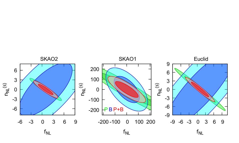
Figure 1: The marginalized $1$ and $2\sigma$ error contours on $(f_{\rm NL},n_{\rm NL}^{\rm s})$ in the single-source model for SKAO2 (left), SKAO1 (middle) and Euclid (right). For each panel, the cases with power spectrum alone (green), bispectrum alone (blue), combined analyses (red) are shown.

Let us consider the single-source model, which was discussed in Sec. 2.2.1. Since we can take $n_{\rm NL}^{\rm m}=0$ and $\tau_{\rm NL}$ can be rewritten in terms of $f_{\rm NL}$ and $n_{\rm NL}^{\rm s}$, the number of independent parameters can reduce to four, $(f_{\rm NL},n_{\rm NL}^{\rm s},g_{\rm NL},n_{\rm NL}^{\rm g})$. In order to simplify the analysis, we further assume that only $f_{\rm NL}$ and $n_{\rm NL}^{\rm s}$ are taken into account. The two-dimensional error contours on $(f_{\rm NL},n_{\rm NL}^{\rm s})$ are shown in Fig. 1, and the marginalized (unmarginalized) $1\sigma$ errors on them are summarized in Table 1. These figure and table imply that the expected constraints from the galaxy power spectrum alone provide a severe degeneracy between $f_{\rm NL}$ and $n_{\rm NL}^{\rm s}$, hence the marginalized constraint are substantially degraded, compared to the unmarginalized ones. This can be understood as follows: As shown in Sec. 3.1, $n_{\rm NL}^{\rm s}$ does not give any scale-dependence to the bias factor of the galaxy power spectrum, but there appears a weak dependence of $n_{\rm NL}^{\rm s}$ on the effective variation of the smoothed density fluctuations. On the other hand, as for the large-scale galaxy bispectrum, although its constraining power is relatively weak, there is a clear scale-dependence with the power-law index $n_{\rm NL}^{\rm s}$. Therefore, we found that it would be useful to use the information of the galaxy bispectrum to break the degeneracy between them and obtain the tighter constraints on both $f_{\rm NL}$ and $n_{\rm NL}^{\rm s}$.

SKAO2	$P$ alone	$B$ alone	$P+B$ combined
$\sigma(f_{\rm NL})$	$1.7(0.48)$	$4.8(3.3)$	$1.4(0.47)$
$\sigma(n_{\rm NL}^{\rm s})$	$1.4(0.38)$	$6.0(3.8)$	$1.1(0.38)$
SKAO1	$P$ alone	$B$ alone	$P+B$ combined
$\sigma(f_{\rm NL})$	$1.5\times 10^{2}(45)$	$1.0\times 10^{2}(58)$	$85(36)$
$\sigma(n_{\rm NL}^{\rm s})$	$1.1\times 10^{2}(31)$	$1.1\times 10^{2}(70)$	$64(28)$
Euclid	$P$ alone	$B$ alone	$P+B$ combined
$\sigma(f_{\rm NL})$	$3.7(0.54)$	$8.6(4.4)$	$2.2(0.53)$
$\sigma(n_{\rm NL}^{\rm s})$	$3.0(0.43)$	$9.8(4.7)$	$1.8(0.43)$

Table 1: Forecast results of marginalized (unmarginalized) $1\sigma$ errors on primordial non-Gaussianity parameters for the case of the single-source model, which is discussed in Sec. 2.2.1.

Next, we consider the model of the generic scale-dependent primordial non-Gaussianities, in which six independent parameters are considered. In Table 2, we summarize the marginalized (unmarginalized) errors on $(f_{\rm NL},n_{\rm NL}^{\rm s},n_{\rm NL}^{\rm m},\tau_{\rm NL},g_{\rm NL},n_{\rm NL}^{\rm g})$. There still exists the degeneracy among these parameters for the case of the galaxy power spectrum in some complicated way. Unfortunately, the parameter degeneracy also appears for the galaxy bispectrum, and the constraining power becomes worse. However, the combined analysis between the galaxy power spectrum and bispectrum can be used to break the parameter degeneracy and obtain the tighter constraints.

SKAO2	$P$ alone	$B$ alone	$P+B$ combined
$\sigma(f_{\rm NL})$	$11(0.53)$	$18(3.4)$	$3.5(0.53)$
$\sigma(n_{\rm NL}^{\rm s})$	$7.9(0.38)$	$10(3.8)$	$1.5(0.38)$
$\sigma(n_{\rm NL}^{\rm m})$	$1.3(0.20)$	$7.1(0.84)$	$1.1(0.19)$
$\sigma(\tau_{\rm NL})$	$38(11)$	$5.7\times 10^{2}(2.1\times 10^{2})$	$33(11)$
$\sigma(g_{\rm NL})$	$1.3\times 10^{6}(5.7\times 10^{4})$	$9.5\times 10^{3}(2.7\times 10^{3})$	$8.7\times 10^{3}(2.7\times 10^{3})$
$\sigma(n_{\rm NL}^{\rm g})$	$1.9\times 10^{5}(8.0\times 10^{3})$	$6.4\times 10^{3}(1.9\times 10^{3})$	$5.8\times 10^{3}(1.8\times 10^{3})$
SKAO1	$P$ alone	$B$ alone	$P+B$ combined
$\sigma(f_{\rm NL})$	$9.5\times 10^{2}(45)$	$1.9\times 10^{2}(59)$	$1.2\times 10^{2}(36)$
$\sigma(n_{\rm NL}^{\rm s})$	$9.4\times 10^{2}(31)$	$1.9\times 10^{3}(69)$	$1.1\times 10^{2}(28)$
$n_{\rm NL}^{\rm m}$	$88(35)$	$1.4\times 10^{2}(35)$	$71(25)$
$\sigma(\tau_{\rm NL})$	$1.5\times 10^{5}(4.8\times 10^{4})$	$2.0\times 10^{5}(5.7\times 10^{4})$	$1.1\times 10^{5}(3.7\times 10^{4})$
$\sigma(g_{\rm NL})$	$3.5\times 10^{7}(1.2\times 10^{6})$	$9.6\times 10^{5}(2.3\times 10^{5})$	$6.8\times 10^{5}(2.3\times 10^{5})$
$\sigma(n_{\rm NL}^{\rm g})$	$7.0\times 10^{6}(1.8\times 10^{5})$	$6.5\times 10^{5}(1.6\times 10^{5})$	$3.9\times 10^{5}(1.2\times 10^{5})$
Euclid	$P$ alone	$B$ alone	$P+B$ combined
$\sigma(f_{\rm NL})$	$27(0.61)$	$29(4.6)$	$4.5(0.61)$
$\sigma(n_{\rm NL}^{\rm s})$	$11(0.43)$	$15(4.7)$	$2.2(0.43)$
$\sigma(n_{\rm NL}^{\rm m})$	$1.6(0.22)$	$11(1.0)$	$1.4(0.22)$
$\sigma(\tau_{\rm NL})$	$47(11)$	$7.6\times 10^{2}(2.4\times 10^{2})$	$36(10)$
$\sigma(g_{\rm NL})$	$6.8\times 10^{6}(1.5\times 10^{5})$	$2.1\times 10^{4}(3.1\times 10^{3})$	$2.1\times 10^{4}(3.1\times 10^{3})$
$\sigma(n_{\rm NL}^{\rm g})$	$5.4\times 10^{5}(2.3\times 10^{4})$	$1.6\times 10^{4}(2.4\times 10^{3})$	$1.6\times 10^{4}(2.4\times 10^{3})$

Table 2: Forecast results of marginalized (unmarginalized) $1\sigma$ errors on primordial non-Gaussianity parameters for the case of the generic model.

5 Summary

We have revisited the local-type primordial non-Gaussianities and have developed the formalism which allows us to include their scale-dependence due to the evolution of the scalar field perturbations after horizon exit and the different scale-dependence of various fields, based on the $\delta N$ formalism. We then have derived the generalized form of the local type bi- and tri-spectra [Eqs. (23)–(26), (29)–(34)]. Although the results are generic formulae, these are a bit complicated and may not be suitable to compare with observational data. Therefore, we have proposed simpler but phenomenologically meaningful expressions, Eqs. (35)–(37), which capture a wide range of physically motivated models. We then have applied our formulae to the specific models, and explicitly shown that not only the amplitude but also the scale-dependence of the primordial non-Gaussianities can be well parametrized by using the generalized local-form.

To see the clustering features of density field caused by the resultant scale-dependent primordial non-Gaussianities, adopting the integrated perturbation theory which systematically includes the late-time gravitational evolution of the effect of halo/galaxy bias, we have derived the formulae of the large-scale power spectrum and bispectrum of the biased objects. We have shown that the scale-dependence of the bias factor for the biased power spectrum is determined only by the power-law index characterizing the multi-field model, $n_{\rm NL}^{\rm m}$, hence the biased power spectrum analysis cannot accurately constrain the power-law indexes characterizing the single-source model, $n_{\rm NL}^{\rm s}$ and $n_{\rm NL}^{\rm g}$. In contrast, the biased bispectrum generated from the primordial one explicitly depends on $n_{\rm NL}^{\rm s}$ and $n_{\rm NL}^{\rm g}$, therefore the combined analysis with the biased power and bi-spectra provides the unique opportunity to probe the scale-dependence of the primordial non-Gaussianities.

Performing the Fisher analysis based on the derived formulae, we have given the forecasts for constraints from the two representative surveys such as SKAO and Euclid. In the case of the single-source model, the measurements of galaxy power spectrum alone provides a severe degeneracy between $f_{\rm NL}$ and $n_{\rm NL}^{\rm s}$, and the marginalized constraint is substantially degraded, compared to the unmarginalized ones. When the galaxy bispectrum is taken into account, there is no serious parameter degeneracy between them and the marginalized constraint on $n_{\rm NL}^{\rm s}$ approaches to the unmarginalized one.

In this paper, we have made several simplified assumptions. In particular, we have considered only the large-scale asymptotes of the biased power spectrum and bispectrum. In this sense, our results presented in this paper may be regarded as a conservative estimate, and a possibility to further improve the constraints needs to be investigated for a quantitative estimation. On the other hand, we have adopted the Limber-approximation for angular power spectrum and bispectrum as statistical quantities. The Limber approximation becomes invalid at lower multipoles, and our treatment with flat-sky limit may not be adequate. This may be a rather optimistic assumption, however the primary purpose of this paper is to explore the impact of the scale-dependence of the local-type primordial non-Gaussianities on future large-scale structure observations. Hence the full-sky correction at lower multipoles to the galaxy power and bi-spectra is left as a future issue.

This work was supported in part by JSPS KAKENHI Grant Nos. 17K14304 (D.Y.), 19H01891 (D.Y.), JP20H01932 (S.Y.), JP20K03968 (S.Y.), 17H01131 (T.T.) and 19K03874 (T.T.), and MEXT KAKENHI Grant No. 19H05110 (T.T.).

Appendix A Explicit form of coefficients

The explicit expressions of the coefficients of the super-horizon scalar field perturbations in Eqs. (10)–(12) are given by (Byrnes et al., 2010b)

$$\epsilon_{IJ}=2\sqrt{\epsilon_{I}\epsilon_{J}}-\eta_{IJ}\,,$$ (103)

$$F^{I}_{(2)JK}=-\frac{V_{IJK}}{3H^{2}}-4\sqrt{2\epsilon_{I}\epsilon_{J}\epsilon_{K}}+\eta_{IJ}\sqrt{2\epsilon_{K}}+\eta_{JK}\sqrt{2\epsilon_{I}}+\eta_{IK}\sqrt{2\epsilon_{J}}\,,$$ (104)

$$F^{I}_{(3)JKL}=-\frac{V_{IJKL}}{3H^{2}}+\sqrt{2\epsilon_{L}}\frac{V_{IJK}}{3H^{2}}+\sqrt{2\epsilon_{K}}\frac{V_{IJL}}{3H^{2}}+\sqrt{2\epsilon_{J}}\frac{V_{IKL}}{3H^{2}}+\sqrt{2\epsilon_{I}}\frac{V_{JKL}}{3H^{2}}$$

$$\quad\quad\quad\quad\quad\quad+24\sqrt{\epsilon_{I}\epsilon_{J}\epsilon_{K}\epsilon_{L}}-4\left(\eta_{IK}\sqrt{\epsilon_{J}\epsilon_{K}}+\eta_{JL}\sqrt{\epsilon_{I}\epsilon_{K}}+\eta_{KL}\sqrt{\epsilon_{I}\epsilon_{J}}\right)$$

$$\quad\quad\quad\quad\quad\quad+\eta_{IJ}\eta_{KL}+\eta_{JK}\eta_{IK}+\eta_{IK}\eta_{JL}\,.$$ (105)

Here we have introduced the slow-roll parameters as $\epsilon=-\dot{H}/H^{2}$, $\epsilon_{I}=(V_{I}/3H^{2})^{2}/2$, and $\eta_{IJ}=V_{IJ}/3H^{2}$.

Appendix B Integrated perturbation theory

In the iPT framework developed in (Matsubara, 2011, 2012), the power spectrum and bispectrum of the biased tracer are constructed with multipoint propagators of the biased object ${\rm X}$ in the Eulerian space, $\Gamma_{\rm X}^{(n)}$, which are defined by the ensemble averages of the functional derivatives

$$\left\langle\frac{\delta^{n}\delta_{\rm X}({\bf k})}{\delta\delta_{\rm L}({\bf k}_{1})\cdots\delta\delta_{\rm L}({\bf k}_{n})}\right\rangle=(2\pi)^{3(1-n)}\delta_{\rm D}^{3}({\bf k}_{1}+\cdots+{\bf k}_{n}-{\bf k})\Gamma_{\rm X}^{(n)}({\bf k}_{1},\cdots,{\bf k}_{n})\,,$$ (106)

where $\delta_{\rm L}$ and $\delta_{\rm X}$ denote the linear density field defined in Eq. (58) and the number density field of the biased objects in Eulerian space, respectively, The first- and second-order multipoint propagators can be described as

$$\Gamma_{\rm X}^{(1)}({\bf k})\approx 1+c_{1}^{\rm L}({\bf k})\,,$$ (107)

$$\Gamma_{\rm X}^{(2)}({\bf k}_{1},{\bf k}_{2})\approx F_{2}({\bf k}_{1},{\bf k}_{2})+\left(1+\frac{{\bf k}_{1}\cdot{\bf k}_{2}}{k_{1}^{2}}\right)c_{1}^{\rm L}({\bf k}_{1})+\left(1+\frac{{\bf k}_{1}\cdot{\bf k}_{2}}{k_{2}^{2}}\right)c_{1}^{\rm L}({\bf k}_{2})+c_{2}^{\rm L}({\bf k}_{1},{\bf k}_{2})\,,$$ (108)

where $F_{2}$ and $c_{n}^{\rm L}$ are the second-order kernel of the standard perturbation theory and the renormalized bias functions in the Lagragian space. To proceed the analysis, we need the explicit expression of the renormalized bias functions. We then adopt the halo bias prescription proposed in (Matsubara, 2012). In this prescription, the renormalized bias function for halos with mass $M$ can be obtained by the universal mass function, $f_{\rm MF}(\nu)$ with $\nu=\delta_{\rm c}/\sigma(M)$ through

$$c_{n}^{\rm L}({\bf k}_{1},\cdots,{\bf k}_{n})=\frac{1}{\nu^{n}}\left(A_{n}(M)+A_{n-1}(M)\frac{\mathrm{d}}{\mathrm{d}\ln\sigma}\right)\left(\frac{W(k_{1}R)\cdots W(k_{n}R)}{\sigma^{n}}\right)\,.$$ (109)

Here a function $A_{n}(M)$ is defined as

$$A_{n}(M)=\sum_{j=0}^{n}\frac{n!}{j!}\frac{(-\nu)^{j}}{f_{\rm MF}(\nu)}\frac{\mathrm{d}^{j}f_{\rm MF}(\nu)}{\mathrm{d}\nu^{j}}\,.$$ (110)

The halo mass function $n_{\rm h}(M)$ and the scale-independent Lagrangian bias function $b_{n}^{\rm L}(M)$ can be defined in terms of the universal mass function as

$$n(M)=-\frac{\rho_{{\rm m},0}}{M^{2}}\frac{\mathrm{d}\ln\sigma}{\mathrm{d}\ln M}f_{\rm MF}(\nu)\,,$$ (111)

$$b_{n}^{\rm L}(M)=\frac{1}{(-\sigma)^{n}f_{\rm MF}}\frac{\mathrm{d}^{n}}{\mathrm{d}\nu^{n}}f_{\rm MF}(\nu)\,.$$ (112)

One can confirm that the long wavelength asymptotes of the renormalized bias functions reduce to the bias defined above, namely $c_{n}^{\rm L}(|{\bf k}_{i}|\to 0)\to b_{n}^{\rm L}$. In this paper, we employ the Sheth-Tormen fitting formula (Sheth, Mo, and Tormen, 2001) for the universal mass function, which is given by

$$f_{\rm MF}(\nu)=A\sqrt{\frac{2q}{\pi}}\left(1+(q\nu^{2})^{-p}\right)\nu e^{-q\nu^{2}/2}\,,$$ (113)

with $A=[1+\Gamma(1/2-p)/\sqrt{\pi}2^{p}]^{-1}$ , $p=0.3$ , and $q=0.707$. When the power spectrum and bispectrum of galaxy clustering are considered, the detailed amplitude and shape of scale-dependent biases depend on the first three functions of the renormalized bias functions, $c_{1}^{\rm L}({\bf k})$, $c_{2}^{\rm L}({\bf k}_{1},{\bf k}_{2})$, and $c_{3}^{\rm L}({\bf k}_{1},{\bf k}_{2},{\bf k}_{3})$. In particular, the coefficients of the bias parameters $A_{1}$, $A_{2}$, and $A_{3}$ are explicitly written in terms of the parameters of the Sheth-Tormen mass functions as

$$A_{1}(M)=q\nu^{2}+\frac{2p}{1+(q\nu^{2})^{p}}\,,$$ (114)

$$A_{2}(M)=q\nu^{2}\delta_{\rm c}b_{1}^{\rm L}(M)+\frac{2p(q\nu^{2}+2p+1)}{1+(q\nu^{2})^{p}}\,,$$ (115)

$$A_{3}(M)=q\nu^{2}\delta_{\rm c}^{2}b_{2}^{\rm L}(M)+\frac{2p[2p(2q\nu^{2}+2p+3)+q^{2}\nu^{4}+q\nu^{2}+2]}{1+(q\nu^{2})^{p}}\,.$$ (116)

We also write down the Lagrangian bias functions as

$$b_{1}^{\rm L}(M)=\frac{1}{\delta_{\rm c}}\left(q\nu^{2}-1+\frac{2p}{1+(q\nu^{2})^{p}}\right)\,,$$ (117)

$$b_{2}^{\rm L}(M)=\frac{1}{\delta_{\rm c}^{2}}\left(q^{2}\nu^{4}-3q\nu^{2}+\frac{2p(2q\nu^{2}+2p-1)}{1+(q\nu^{2})^{p}}\right)\,,$$ (118)

$$b_{3}^{\rm L}(M)=\frac{1}{\delta_{\rm c}^{3}}\left(q^{3}\nu^{6}-6q^{2}\nu^{4}+3q\nu^{2}+\frac{2p[2p(3q\nu^{2}+2p)+3q^{2}\nu^{4}-6q\nu^{2}-1]}{1+(q\nu^{2})^{p}}\right)\,.$$ (119)

References

• Komatsu and Spergel (2001) E. Komatsu and D. N. Spergel, Phys. Rev. D 63, 063002 (2001) doi:10.1103/PhysRevD.63.063002 [arXiv:astro-ph/0005036 [astro-ph]].
• Starobinsky (1986) A. A. Starobinsky, JETP Lett. 42, 152-155 (1985)
• Salopek and Bond (1990) D. S. Salopek and J. R. Bond, Phys. Rev. D 42, 3936-3962 (1990) doi:10.1103/PhysRevD.42.3936
• Sasaki and Stewart (1995) M. Sasaki and E. D. Stewart, Prog. Theor. Phys. 95, 71-78 (1996) doi:10.1143/PTP.95.71 [arXiv:astro-ph/9507001 [astro-ph]].
• Sasaki and Tanaka (1998) M. Sasaki and T. Tanaka, Prog. Theor. Phys. 99, 763-782 (1998) doi:10.1143/PTP.99.763 [arXiv:gr-qc/9801017 [gr-qc]].
• Lyth, Malik, and Sasaki (2004) D. H. Lyth, K. A. Malik and M. Sasaki, JCAP 05, 004 (2005) doi:10.1088/1475-7516/2005/05/004 [arXiv:astro-ph/0411220 [astro-ph]].
• Lyth and Rodriguez (2005) D. H. Lyth and Y. Rodriguez, Phys. Rev. Lett. 95, 121302 (2005) doi:10.1103/PhysRevLett.95.121302 [arXiv:astro-ph/0504045 [astro-ph]].
• Akrami et al. (2018) Y. Akrami et al. [Planck], Astron. Astrophys. 641, A9 (2020) doi:10.1051/0004-6361/201935891 [arXiv:1905.05697 [astro-ph.CO]].
• Dalal et al. (2008) N. Dalal, O. Dore, D. Huterer and A. Shirokov, Phys. Rev. D 77, 123514 (2008) doi:10.1103/PhysRevD.77.123514 [arXiv:0710.4560 [astro-ph]].
• Desjacques, Seljak, and Iliev (2209) V. Desjacques, U. Seljak and I. Iliev, Mon. Not. Roy. Astron. Soc. 396, 85-96 (2009) doi:10.1111/j.1365-2966.2009.14721.x [arXiv:0811.2748 [astro-ph]].
• Bacon et al. (2020) D. J. Bacon et al. [SKA], Publ. Astron. Soc. Austral. 37, e007 (2020) doi:10.1017/pasa.2019.51 [arXiv:1811.02743 [astro-ph.CO]].
• Yamauchi et al. (2016) D. Yamauchi et al. [SKA-Japan Consortium Cosmology Science Working Group], Publ. Astron. Soc. Jap. 68, no.6, R2 (2016) doi:10.1093/pasj/psw098 [arXiv:1603.01959 [astro-ph.CO]].
• Ferramacho et al. (2014) L. D. Ferramacho, M. G. Santos, M. J. Jarvis and S. Camera, Mon. Not. Roy. Astron. Soc. 442, no.3, 2511-2518 (2014) doi:10.1093/mnras/stu1015 [arXiv:1402.2290 [astro-ph.CO]].
• Yamauchi, Takahashi, and Oguri (2014) D. Yamauchi, K. Takahashi and M. Oguri, Phys. Rev. D 90, no.8, 083520 (2014) doi:10.1103/PhysRevD.90.083520 [arXiv:1407.5453 [astro-ph.CO]].
• Yamauchi and Takahashi (2015) D. Yamauchi and K. Takahashi, Phys. Rev. D 93, no.12, 123506 (2016) doi:10.1103/PhysRevD.93.123506 [arXiv:1509.07585 [astro-ph.CO]].
• de Putter and Doré (2014) R. de Putter and O. Doré, Phys. Rev. D 95, no.12, 123513 (2017) doi:10.1103/PhysRevD.95.123513 [arXiv:1412.3854 [astro-ph.CO]].
• Jeong and Komatsu (2009) D. Jeong and E. Komatsu, Astrophys. J. 703, 1230-1248 (2009) doi:10.1088/0004-637X/703/2/1230 [arXiv:0904.0497 [astro-ph.CO]].
• Hashimoto et al. (2016) I. Hashimoto, A. Taruya, T. Matsubara, T. Namikawa and S. Yokoyama, Phys. Rev. D 93, no.10, 103537 (2016) doi:10.1103/PhysRevD.93.103537 [arXiv:1512.08352 [astro-ph.CO]].
• Tellerini et al. (2016) M. Tellarini, A. J. Ross, G. Tasinato and D. Wands, JCAP 06, 014 (2016) doi:10.1088/1475-7516/2016/06/014 [arXiv:1603.06814 [astro-ph.CO]].
• Yamauchi, Yokoyama, and Takahashi (2016) D. Yamauchi, S. Yokoyama and K. Takahashi, Phys. Rev. D 95, no.6, 063530 (2017) doi:10.1103/PhysRevD.95.063530 [arXiv:1611.03590 [astro-ph.CO]].
• Shirasaki et al. (2021) M. Shirasaki, N. S. Sugiyama, R. Takahashi and F. S. Kitaura, Phys. Rev. D 103, no.2, 023506 (2021) doi:10.1103/PhysRevD.103.023506 [arXiv:2010.04567 [astro-ph.CO]].
• Yamauchi, Yokoyama, and Tashiro (2017) D. Yamauchi, S. Yokoyama and H. Tashiro, Phys. Rev. D 96, no.12, 123516 (2017) doi:10.1103/PhysRevD.96.123516 [arXiv:1709.03243 [astro-ph.CO]].
• Yamauchi and Sugiyama (2021) D. Yamauchi and N. S. Sugiyama, [arXiv:2108.02382 [astro-ph.CO]].
• Suyama et al. (2010) T. Suyama, T. Takahashi, M. Yamaguchi and S. Yokoyama, JCAP 12, 030 (2010) doi:10.1088/1475-7516/2010/12/030 [arXiv:1009.1979 [astro-ph.CO]].
• Yokoyama, Suyama, and Tanaka (2007a) S. Yokoyama, T. Suyama and T. Tanaka, JCAP 07 (2007), 013 doi:10.1088/1475-7516/2007/07/013 [arXiv:0705.3178 [astro-ph]].
• Yokoyama, Suyama, and Tanaka (2007b) S. Yokoyama, T. Suyama and T. Tanaka, Phys. Rev. D 77 (2008), 083511 doi:10.1103/PhysRevD.77.083511 [arXiv:0711.2920 [astro-ph]].
• Byrnes et al. (2010a) C. T. Byrnes, S. Nurmi, G. Tasinato and D. Wands, JCAP 02 (2010), 034 doi:10.1088/1475-7516/2010/02/034 [arXiv:0911.2780 [astro-ph.CO]].
• Byrnes et al. (2010b) C. T. Byrnes, M. Gerstenlauer, S. Nurmi, G. Tasinato and D. Wands, JCAP 10 (2010), 004 doi:10.1088/1475-7516/2010/10/004 [arXiv:1007.4277 [astro-ph.CO]].
• Byrnes and Gong (2012) C. T. Byrnes and J. O. Gong, Phys. Lett. B 718, 718-721 (2013) doi:10.1016/j.physletb.2012.11.052 [arXiv:1210.1851 [astro-ph.CO]].
• Byrnes, Enqvist, and Takahashi (2010) C. T. Byrnes, K. Enqvist and T. Takahashi, JCAP 09, 026 (2010) doi:10.1088/1475-7516/2010/09/026 [arXiv:1007.5148 [astro-ph.CO]].
• Huang (2010a) Q. G. Huang, JCAP 11, 026 (2010) [erratum: JCAP 02, E01 (2011)] doi:10.1088/1475-7516/2011/02/E01 [arXiv:1008.2641 [astro-ph.CO]].
• Huang (2010b) Q. G. Huang, JCAP 12, 017 (2010) doi:10.1088/1475-7516/2010/12/017 [arXiv:1009.3326 [astro-ph.CO]].
• Byrnes et al. (2011) C. T. Byrnes, K. Enqvist, S. Nurmi and T. Takahashi, JCAP 11, 011 (2011) doi:10.1088/1475-7516/2011/11/011 [arXiv:1108.2708 [astro-ph.CO]].
• Huang and Lin (2011) Q. G. Huang and C. Lin, JCAP 10, 005 (2011) doi:10.1088/1475-7516/2011/10/005 [arXiv:1108.4474 [astro-ph.CO]].
• Kobayashi and Takahashi (2012) T. Kobayashi and T. Takahashi, JCAP 06, 004 (2012) doi:10.1088/1475-7516/2012/06/004 [arXiv:1203.3011 [astro-ph.CO]].
• Byrnes and Tarrant (2015) C. T. Byrnes and E. R. M. Tarrant, JCAP 07, 007 (2015) doi:10.1088/1475-7516/2015/07/007 [arXiv:1502.07339 [astro-ph.CO]].
• Becker and Huterer (2012) A. Becker and D. Huterer, Phys. Rev. Lett. 109, 121302 (2012) doi:10.1103/PhysRevLett.109.121302 [arXiv:1207.5788 [astro-ph.CO]].
• Oppizzi et al. (2018) F. Oppizzi, M. Liguori, A. Renzi, F. Arroja and N. Bartolo, JCAP 05, 045 (2018) doi:10.1088/1475-7516/2018/05/045 [arXiv:1711.08286 [astro-ph.CO]].
• Dai and Xia (2020) J. P. Dai and J. Q. Xia, Mon. Not. Roy. Astron. Soc. 491, no.1, L61-L65 (2020) doi:10.1093/mnrasl/slz170 [arXiv:1911.01329 [astro-ph.CO]].
• Raccanelli, Dore, and Dalal (2014) A. Raccanelli, O. Dore and N. Dalal, JCAP 08, 034 (2015) doi:10.1088/1475-7516/2015/08/034 [arXiv:1409.1927 [astro-ph.CO]].
• Ballardini, Mattherson, and Maartens (2019) M. Ballardini, W. L. Matthewson and R. Maartens, Mon. Not. Roy. Astron. Soc. 489, no.2, 1950-1956 (2019) doi:10.1093/mnras/stz2258 [arXiv:1906.04730 [astro-ph.CO]].
• Sefusatti et al. (2009) E. Sefusatti, M. Liguori, A. P. S. Yadav, M. G. Jackson and E. Pajer, JCAP 12, 022 (2009) doi:10.1088/1475-7516/2009/12/022 [arXiv:0906.0232 [astro-ph.CO]].
• Giannantonio et al. (2012) T. Giannantonio, C. Porciani, J. Carron, A. Amara and A. Pillepich, Mon. Not. Roy. Astron. Soc. 422, 2854-2877 (2012) doi:10.1111/j.1365-2966.2012.20604.x [arXiv:1109.0958 [astro-ph.CO]].
• Becker, Huterer, and Kadota (2012) A. Becker, D. Huterer and K. Kadota, JCAP 12, 034 (2012) doi:10.1088/1475-7516/2012/12/034 [arXiv:1206.6165 [astro-ph.CO]].
• Biagetti et al. (2013) M. Biagetti, H. Perrier, A. Riotto and V. Desjacques, Phys. Rev. D 87, 063521 (2013) doi:10.1103/PhysRevD.87.063521 [arXiv:1301.2771 [astro-ph.CO]].
• Shandera, Dalal, and Huterer (2010) S. Shandera, N. Dalal and D. Huterer, JCAP 03 (2011), 017 doi:10.1088/1475-7516/2011/03/017 [arXiv:1010.3722 [astro-ph.CO]].
• Matsubara (2011) T. Matsubara, Phys. Rev. D 83 (2011), 083518 doi:10.1103/PhysRevD.83.083518 [arXiv:1102.4619 [astro-ph.CO]].
• Matsubara (2012) T. Matsubara, Phys. Rev. D 86 (2012), 063518 doi:10.1103/PhysRevD.86.063518 [arXiv:1206.0562 [astro-ph.CO]].
• Yokoyama and Matsubara (2012) S. Yokoyama and T. Matsubara, Phys. Rev. D 87 (2013), 023525 doi:10.1103/PhysRevD.87.023525 [arXiv:1210.2495 [astro-ph.CO]].
• Yokoyama, Matsubara, and Taruya (2013) S. Yokoyama, T. Matsubara and A. Taruya, Phys. Rev. D 89 (2014) no.4, 043524 doi:10.1103/PhysRevD.89.043524 [arXiv:1310.4925 [astro-ph.CO]].
• Cooray and Sheth (2002) A. Cooray and R. K. Sheth, Phys. Rept. 372 (2002), 1-129 doi:10.1016/S0370-1573(02)00276-4 [arXiv:astro-ph/0206508 [astro-ph]].
• Tinker et al. (2005) J. L. Tinker, D. H. Weinberg, Z. Zheng and I. Zehavi, Astrophys. J. 631 (2005), 41-58 doi:10.1086/432084 [arXiv:astro-ph/0411777 [astro-ph]].
• Conroy, Wechsler, and Kravtsov (2005) C. Conroy, R. H. Wechsler and A. V. Kravtsov, Astrophys. J. 647 (2006), 201-214 doi:10.1086/503602 [arXiv:astro-ph/0512234 [astro-ph]].
• Kayo, Takada, and Jain (2012) I. Kayo, M. Takada and B. Jain, Mon. Not. Roy. Astron. Soc. 429 (2013), 344-371 doi:10.1093/mnras/sts340 [arXiv:1207.6322 [astro-ph.CO]].
• Bull (2016) P. Bull, Astrophys. J. 817 (2016) no.1, 26 doi:10.3847/0004-637X/817/1/26 [arXiv:1509.07562 [astro-ph.CO]].
• Amendola et al. (2018) L. Amendola, S. Appleby, A. Avgoustidis, D. Bacon, T. Baker, M. Baldi, N. Bartolo, A. Blanchard, C. Bonvin and S. Borgani, et al. Living Rev. Rel. 21 (2018) no.1, 2 doi:10.1007/s41114-017-0010-3 [arXiv:1606.00180 [astro-ph.CO]].
• Sheth, Mo, and Tormen (2001) R. K. Sheth, H. J. Mo and G. Tormen, Mon. Not. Roy. Astron. Soc. 323 (2001), 1 doi:10.1046/j.1365-8711.2001.04006.x [arXiv:astro-ph/9907024 [astro-ph]].