Canoe : A System for Collaborative Learning for Neural Nets

Abstract.

For highly distributed environments such as edge computing, collaborative learning approaches eschew the dependence on a global, shared model, in favor of models tailored for each location. Creating tailored models for individual learning contexts reduces the amount of data transfer, while collaboration among peers provides acceptable model performance. Collaboration assumes, however, the availability of knowledge transfer mechanisms, which are not trivial for deep learning models where knowledge isn’t easily attributed to precise model slices. We present Canoe – a framework that facilitates knowledge transfer for neural networks. Canoe provides new system support for dynamically extracting significant parameters from a helper node’s neural network, and uses this with a multi-model boosting-based approach to improve the predictive performance of the target node. The evaluation of Canoe with different PyTorch and TensorFlow neural network models demonstrates that the knowledge transfer mechanism improves the model’s adaptiveness to changes up to $3.5\times$ compared to learning in isolation, while affording several magnitudes reduction in data movement costs compared to federated learning.

1. Introduction

The rise of sensors and connected devices leads to tremendous growth in the amount of data generated at the edges of the network. In order to manage, process and analyze the increasing amount of data, service providers have started relying on machine learning techniques to provide automation and to improve user experience, content discovery, curated search results or recommendations (Hazelwood et al., 2018; Amatriain, 2013; Amat et al., 2018; Neethu and Rajasree, 2013; Syam and Sharma, 2018; Ozertem et al., 2012).

With data been generated in a highly distributed manner, companies build machine learning (ML) models using systems for distributed learning such as Federated Learning (FL) (Konečnỳ et al., 2015; Arivazhagan et al., 2019). Such solutions leverage computational resources closer to the sources, in geo-distributed data centers (Hsieh et al., 2017) or at many distributed server locations in the edges of the network (Wang et al., 2019; Wang et al., 2019; Lu et al., 2019), to learn in place from localized data and summarize the changes as a model update. Model updates from all participants are aggregated in a centralized location to improve a global model, which is then shared with all. FL reduces the data transfer cost compared to approaches which aggregate the raw data centrally, however the communication with a remote cloud is still required for regular exchange of model updates.

In fact, by aiming to build a global, generic model, all of the above approaches rely on periodic communication among distributed locations, in order to transfer raw data or model updates. Highly distributed environments, particularly such as those observed across nodes in mobile edge computing (MEC) (ets, [n.d.]), have been shown to benefit from models tailored to the context of specific locations (Polese et al., 2018; Padmanabha Iyer et al., 2018; Paul et al., 2011a; Zhou et al., 2012a; Daga et al., 2019; Lu et al., 2019). In addition, distinct locations may not exhibit any change in their localized inputs, thus not benefiting from model updates due to churn in data trends observed at other locations. Abandoning any cross-node coordination in learning in favor of isolated learning approaches, eliminates data transfer costs. However, if data trends shift across locations (i.e., in the event of concept drift), models learned in isolation suffer from loss of accuracy and need more time to adapt to change, compared to when relying on a global model. In response, distributed machine learning models for collaborative learning across edge nodes have been proposed, as a way to create robust tailored models. Collaborative learning allows distributed nodes to adapt quickly to input shifts and retain model accuracy, with low data transfer costs (Daga et al., 2019; Lu et al., 2019).

A key assumption in realizing collaborative learning is the ability to transfer knowledge from one peer who has previously learned a given input class – a helper node – to another peer exhibiting a change in its inputs – a target node. For certain types of machine learning models, such as the online random forest (ORF) and online support vector machines (OSVM) used in (Daga et al., 2019), realizing knowledge transfer is straightforward, as the association of input classes to model parameters is easily identifiable: to transfer knowledge about a given class from a helper to a target model, the corresponding subtrees in ORF or matrix rows in OSVM models need to be copied over across models. In practice, however, services are increasingly turning to deep learning techniques based on neural networks (app, [n.d.]; Zheng et al., 2020; fb:, [n.d.]; goo, [n.d.]; Bhatia et al., 2020; Homayounfar et al., 2019; Kaplanyan et al., 2019), where knowledge about a particular input class cannot be trivially attributed to a slice of the model. This raises the question, how to enable knowledge transfer across neural network (NN) models? Without the support to extract features from a helper node’s model relevant for the knowledge needed at the target, and to then integrate them with the target node’s model, collaborative learning will not be feasible for deep learning techniques. This will limit the opportunity for the benefits of collaborative distributed learning to be afforded to many important application classes relying on deep learning.

In response, we present Canoe – a framework that enables collaborative deep learning by facilitating selective knowledge transfer across neural network models. Canoe combines system support for dynamic creation of helper models from an existing neural network model, with a multi-model boosting-based approach to use this knowledge and update a target model. The knowledge transfer in Canoe is made possible through the use of mechanisms for (1) on-demand gleaning of significant parameters of a model, (2) use of boosted helper models, and (3) support for managing helper model chains. Canoe is evaluated for several neural network models based on PyTorch and TensorFlow, and shows opportunities for significant improvements in model performance and data transfer costs, across both frameworks and with different models. The evaluation also demonstrates that Canoe exposes new opportunities to exploit tradeoffs among model accuracy, the ability to quickly adapt to changes in a model’s predictive performance, data transfer costs and learning overheads. Future policy engines can exploit such tradeoffs to further tailor the behavior of the distributed learning process.

In summary, the contributions of this paper include:

• New mechanisms to facilitate knowledge transfer for deep learning models (§5);

• The design and implementation of Canoe, a first framework that integrates support for collaborative deep learning (§6);

• Evaluation with several models, ML frameworks, and workloads, which demonstrates that Canoe enables collaborative deep learning across distributed nodes in a manner that allows models to adapt to change $3.5\times$ faster than isolated learning while giving a similar predictive performance compared to federated learning, but with orders of magnitude lower overall data transfer costs (§7).

2. Background and Motivation

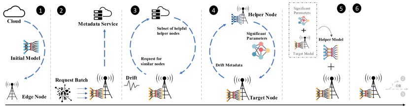
Figure 1. Collaborative learning in distributed edge computing.

Multi-access Edge Computing. MEC (ets, [n.d.]; Sabella et al., 2016) provides IT services and compute capabilities at the edge of the network, in wireless and cellular access points such as gateways and cell towers, in close proximity to the client devices. It offers infrastructure for execution of applications requiring low latency (e.g., AR/VR, automation (Al-Shuwaili and Simeone, 2017; Ren et al., 2019)), reduction in backhaul data demand (e.g., IoT analytics (Li et al., 2018; Satyanarayanan et al., 2015), content delivery (Fajardo et al., 2015; Zhang et al., 2018)), and geo-localized data handling (e.g., for GDPR (Parliament and of the European Union, 2018)). One challenge MEC exposes is that of creating an extremely dispersed distributed infrastructure, which differs from datacenter-based distributed environments in its scale and in the fine-grained geo-localization of the inputs observed at each node (Polese et al., 2018). For instance, COLLA (Lu et al., 2019), a collaborative system to predict user behavior patterns, highlights that a shared global model might not achieve the desired performance for all the users. Thus it trains smaller more tailored models at individual edge nodes and captures users with similar behavior patterns. Cellscope (Padmanabha Iyer et al., 2018) also demonstrated the ineffectiveness of using a shared global model for managing the base stations in mobile network; similar observations are confirmed in other research (Paul et al., 2011a; Zhou et al., 2012a).

Collaborative Distributed Learning. Contrary to federated learning, where a global shared model is created and distributed, collaborative distributed learning is relevant for contexts such as MEC, where information is localized and nodes require only a portion of the global model (Daga et al., 2019; Lu et al., 2019). This helps in reducing the overall data transfer, provides smaller model size and reduces (re)training time.

Figure 1 illustrates a typical workflow in a collaborative system. Edge nodes use their resident model to perform inference, following which the model is re-trained locally. Upon shift in the data distribution, the model performance at the edge node deteriorates. In such a scenario, the node relies on the collaborative system to find a helper node, and to leverage the helper’s model (knowledge) to boost its own model. In order to find a helper node in a timely manner, a common metadata service (MdS) aggregates information from each node in the system. This metadata is information that helps the system differentiate the nodes, such as node hardware, network configuration, workload characteristics such as estimates of class priors, overall model performance, etc. Each edge node uses drift detection algorithms (Gama et al., 2014; Kifer et al., 2004; Bifet and Gavalda, 2007) on the local metadata information to decide when a model at the target edge node needs to be updated, and to query the MdS for candidates for a possible helper. The MdS uses the metadata it has aggregated to determine helper node candidates using algorithms such as (Joyce, 2011; Beran et al., 1977; Rao and Scott, 1981; Lin, 1991).

In order to update the target node’s model and improve its predictive performance, a collaborative system uses knowledge transfer (Daga et al., 2019) or distillation (Lu et al., 2019). Knowledge distillation (Hinton et al., 2015) uses a teacher model to train a student model. It is a process of transferring knowledge from a large model (teacher) to a smaller model (student) to obtain similar accuracy as the teacher model. Knowledge transfer is a mechanism to transfer the knowledge regarding several (typically not all) classes from one machine learning model to another. In this paper we use knowledge transfer mechanism to collaborate among edge nodes which use the same neural network. We chose knowledge transfer over distillation because in distillation the teacher model is assumed to be a perfect model, whereas, we already point out, a perfect global model may not be needed for MEC, and it may be too costly to maintain it at large scale in a highly distributed settings.

Neural Networks for MEC. When compared with other machine learning models, Neural Networks have shown superior performance for many emerging intelligent applications. Convolutional Neural Networks (CNN) (LeCun et al., 1995) have shown best performance for image and video analytics, while Recurrent Neural Networks (RNN) (Zaremba et al., 2014) are extensively used for voice search (Hakkani-Tür et al., 2016) such as Apple’s Siri and Google’s voice search. A growing number of applications based on real-time analytics of sensor data, automation, AR/VR, etc., (Kanzaki et al., 2017; Li et al., 2018; Wang et al., 2017; Bura et al., 2018; Lu et al., 2018; Hou and Dey, 2020; Liu et al., 2019), have started to deploy deep learning services at the edge of the network. The real-time nature of applications makes the inference latency-critical. The large size and distribution of the training data that may be gathered across the user contexts of these applications, make such applications bandwidth intensive. One potential solution is to use federated learning for such applications. However, when working with neural nets even small amounts of raw data can result in large amounts of information being communicated to the aggregating node (Bonawitz et al., 2019). The combination of these factors makes support for collaborative learning for neural network an important distributed learning strategy. This, in turn, requires support for knowledge transfer.

Knowledge Transfer in Neural Networks. Knowledge transfer for neural networks is a hard problem that is receiving a lot of attention from the ML community (Zhou et al., 2018; Bau et al., 2018; Yosinski et al., 2014). Even when considering the same type of neural networks, given the many connected layers, information required to classify a class is spread across each layer, requiring specialized algorithms to extract it. If the data observed at target node is very similar to the one observed by the helper, fine-tuning (Tajbakhsh et al., 2016) is one methodology that can be used, where the helper model design and parameters are fully or partially replicated on the target model. However, as workload characteristics can vary across different nodes, using this technique can further reduce the model performance, as we show in §5.2. One alternative is to improve and speed up the learning of the target node model for the new task using techniques such as  (Parisotto et al., 2015; Xu et al., 2020). However, such techniques assume the helper model to be an expert teacher model, which in our case might not be always feasible. A different approach is to apply techniques that extract the portion of the model that most contribute to its performance for a given input. (Zhou et al., 2018) suggests removing one neuron at a time to determine if it has impact on the model performance. (Yu et al., 2018) analyzes the activation, gradients and visualization patterns to determine a critical path. However, as the machine learning models are continuously (re)trained on the incoming data stream at each edge node, knowledge transfer needs to be performed dynamically, and over fresh models, requiring time and resource-efficient techniques.

3. Goal and Challenges

Goal. The goal of Canoe is to provide a collaborative framework for distributed deep learning which will enable fast knowledge transfer across the neural network models of the peer nodes.

System model. The previous section illustrates that in a collaborative system each edge node creates a customized model and requests for help when there is drift in the model performance. The concept of providing help is the ability to perform knowledge transfer from a helper node to a target node. We assume that helper nodes can be identified from the model and node metadata, using techniques such as (Joyce, 2011; Beran et al., 1977; Rao and Scott, 1981; Lin, 1991), as done in (Daga et al., 2019). The specific contributions made by Canoe are new techniques which enable knowledge transfer to be performed across neural network models among distributed nodes in a manner that boosts the overall accuracy at the target node while maintaining low data transfer costs.

Challenges. The fundamental issue in performing knowledge transfer across collaborative peer nodes lies in the fact that the helper node’s knowledge is neither all necessary at the target node, nor is it strictly a superset of the target node’s knowledge. Simply using the helper node’s model introduces either unnecessary data movement (for portion of the knowledge not relevant for the inputs at the target), or worse, degrades the target node’s knowledge (by displacing localized knowledge that was already acquired). This is in contrast to centralized or federated learning frameworks, where a centralized helper node is assumed to have globally relevant, generic model. Instead, for collaborative learning only a relevant portion of the helper node’s model needs to be transferred, such that the target model can achieve the needed boost in its accuracy, while also keeping the data transfer costs low. Addressing this issue for neural network models introduces the following main challenges:

C1: How to extract a relevant portion of a neural network model? A neural network model consists of multiple hidden layers. It takes an input, passes it through multiple layers of hidden neurons (mini-functions with unique coefficients that must be learned), and outputs a prediction representing the combined input of all the neurons. Thus, various parameters spread across different layers help the model in providing a good predictive performance. The challenge is to determine a methodology that could help in selecting the relevant parameters from all the layers, and to do so with low overheads and with low resulting data transfer demands.

C2: How to utilize the knowledge at the target node? The target node’s neural network similarly consists of hidden layers whose parameter values reflect existing locally acquired knowledge. The model parameters then need to be carefully updated with the knowledge obtained from the helper, in order to improve the target model without displacing local knowledge. The challenge is to determine a methodology for updating the target node’s model parameters with the helper’s knowledge quickly and effectively, without degrading its performance on previously known classes.

4. Overview of Canoe

Approach. To address these challenges, Canoe adopts an approach that combines support to dynamically extract significant model parameters, with use of multi-model boosting. Specifically, Canoe relies on helper nodes, but only extracts the portion of their knowledge relevant for the target node. It then uses boosting to create custom helper models for the target, and then uses those helper models, in conjunction with the target’s existing knowledge, to create a more effective combined model.

By using a multi-model approach, Canoe makes it possible to decouple the updates that need to be performed to improve the target model’s prediction accuracy from the specific parameters extracted from the helper node’s original model. By using a simple boosting technique to create the helper models, Canoe makes it possible to achieve a resulting helper model that benefits from the helper for recognizing new classes, while retaining its knowledge quality for pre-existing, familiar classes.

Mechanisms. Underpinning Canoe are three key mechanisms designed for selecting significant parameters from the helper node’s model, creating a boosted helper model and managing model chains on the target node.

To solve the challenge C1 of selectively picking the parameters from each layer of the neural network, the framework uses a mechanism for significant parameter selection, in Figure 1. The task of selecting significant parameters of a DNN model can be rephrased into the following question: given a DNN $f$ and input image $x$, what is the part of $f(x)$ that made the DNN reach the particular decision of classifying the input as class $y$. In other words, which coefficients or weights at each layer in the model contributed towards the classification of $x$ to an output $y$?

On the target node, Canoe creates helper models using the significant parameters from the original model  . A helper model with poor performance for some classes can degrade the overall model performance, effectively displacing knowledge that already existed as part of the target model. To prevent this, a helper model should be created by using the knowledge obtained from the helper node with the existing knowledge on the target node. The resulting helper model is then used in conjunction with target model.

A target node may exhibit multiple instance of input drift over time. This will require new knowledge transfers, and can result in a chain of helper models. To prevent helper models from creating a resource bloat on the target, they are ephemeral, and are discarded when no longer needed. The target node continues to learn during the boosting period, so as to make it possible to remove its dependence on the helper model. Once all helper models are discarded, the target continues to operate only with its, now updated, target model . The use of a boosted helper model and the techniques for managing helper model chains, solve the challenge C2.

5. Design of Canoe

Next, we describe in greater detail the design of the three mechanisms Canoe uses to realize knowledge transfer from a helper to a target node for neural network models.

5.1. Significant Parameters Selection

To address the challenge C1, Canoe provides support for extracting a relevant portion of a helper node’s model in a practical manner via a mechanism for selecting the model’s significant parameters. A neural network model consists of multiple hidden layers of neurons, each with their activation function, interconnected with weighted synapses. During the learning process each neuron takes a group of weighted input, applies an activation function and returns the output. These inputs can be features from the dataset or output of a previous layer’s neuron. The weights are adjusted using backpropagation (Hecht-Nielsen, 1992) (”backprop”), and the process is repeated until the network error drops below a threshold. Thus, for a given input, a combination of coefficients across multiple layers plays a role in determining the outcome. Our goal is to select from each layer of a model the significant parameters that are relevant to the requested classes.

A trivial design choice could be to send the entire model from a helper to a target node while avoiding any overhead of selecting a relevant portion of the helper model. However, this is not a good design choice as NN models are large, and can include millions of parameters as shown in Table 1. Furthermore, when considering collaborative learning, only certain parameters relevant for the missing classes are required by the target node. Thus, by pre-processing the helper’s node original model to identify and send only the significant parameters for the relevant classes, the data transfer cost are reduced.

Parameter Sensitivity. To select the significant parameters we first need to determine the relation and influence of each parameter on the output value, i.e., the parameter sensitivity. A neural network consists of a large number of parameters. A change in the value of these parameters has a direct impact on the predictive performance of the model. Our goal is to first understand the sensitivity and impact of each parameter on the output value, and then to determine a subset of the most significant parameters. We use the backprop technique to determine the sensitivity by finding the impact that a small change in an input neuron (i) has on an output neuron (o). If drastic change occurs, i is considered to be significant for producing the current activation value of o.

Let $f(W,x)=p$ denote the neural network model where $W$, $x$ and $p$ are set of all the model parameters, inputs and prediction, respectively. For a multi-class classification task the output of the neural network is an array of size $C$ where each element represents the confidence of the input being class $C_{i}$. We determine the sensitivity value of a parameter $W_{j}$ towards the class output value $C_{i}$ as

(1) $$sen(W_{j},C_{i})=\frac{\partial C_{i}}{\partial W_{j}}=\lim\limits_{\Delta W_{j}\rightarrow 0}\frac{C_{i}(W_{j}+\Delta W_{j})-C_{i}(W_{j})}{\Delta W_{j}}$$

$sen(W_{j},C_{i})>0$ means increasing the value of parameter $W_{j}$, increases the output value for class $C_{i}$ which implies the model is more confident that the input belongs to class $C_{i}$. On the contrary, $sen(W_{j},C_{i})<0$ means increasing $W_{j}$ makes the model more confident about an input not being class $C_{i}$. Thus, $|sen(W_{j},C_{i})|$ is defined as the measure of sensitivity of the parameter. The larger magnitude indicates higher significance of the parameter, as a small change in the parameter value could change the output.

Calculating the sensitivity value of each parameter for all the classes is computational expensive. Thus for a class the sensitivity of each parameter is calculated using the backprop technique similar to the one used in gradient descent (Amari, 1993) where it uses the partial derivative to determine the impact of change of the parameter on the class output value.

Determining sensitivity for a changing model. Over time the model at the edge node changes. As a result significant values cannot be calculated in the initial phase and used at a later time when a request from the target node is received. As the model is continuously retrained there are few ways to evaluate these values (Zhou et al., 2018; Cao and Chen, 1997; Zeng and Yeung, 2001; Amari, 1998). We can either pre-calculate the sensitivity after every batch in a continuous manner, and then do a quick look up when a request from a target node is received, or dynamically compute these values upon request. To evaluate the contribution of parameters on-demand, we can either add Gaussian noise at different layers (Rusu et al., 2016) or have a data reservoir and use the backprop technique to measure how their change contributes to the model output ($o$).

The first method is based on a continuous update of a sensitivity map for all model parameters and classes. Since the gradient is linear we combine the neural net output of all the data points in a batch to compute the parameters sensitivity value for all the classes. For the subsequent batches the values are recalculated and are added with the previously stored values. After every batch, this calculation of parameters adds a compute overhead of up to $0.7\times$ the time taken to process a batch. Additionally, since the sensitivity value of a parameter is different from its actual value in the model, this approach requires an addition memory of $O(CW)$ at each edge node. With large NN model sizes and resource constrained edge nodes, this method might not be a viable option. However, the pre-calculated values help in quickly responding to the request when a request for a portion of the model is made.

A second approach is one where significant parameters are calculated on-demand, when a request is received. To achieve this we keep a smaller local database (data reservoir) of the last $B$ request batches. When requested, the sensitivity of the parameters is calculated against the stored batches in a similar way as before. The effectiveness and overheads of this method are dependent on the exact setting of $B$. In general, the choice depends on the workload dynamics and model. For our dataset and models we experimentally found that $B=1$ worked well as each request batch consists of sufficient data points.

The above two approaches showcase a tradeoff between the amount of memory required to calculate the sensitivity parameters and response time. §7.3 discusses the overhead involved in each of the approaches. Canoe provides a pluggable parameter selection component which enables the user to use any technique.

Significant Parameters. Once the helper node determines the sensitivity of the parameters for the requested classes, the system selects the top $Z$ percent of the sensitive parameter (both positive and negative). For a multi-class request we average the sensitivity value for all the classes before selecting the top $Z$ parameters. After selecting the top parameters, Canoe selects the corresponding weights of these parameters from the model. Since these parameters are the most relevant towards the classification of a class we refer to them as significant parameters. The significant parameters are compressed, which reduces the data size by up to $3$-$5\times$, and are sent to the target node. The exact setting of $Z$ depends on the model as well as the tradeoff between the data transfer versus knowledge transfer to improve the target node model. For our dataset and NN models we experimentally found that $Z$ can vary in the range $20\%$ to $50\%$. §7.4 illustrates the impact of different values of $Z$ and we leave the automatic tuning of $Z$ as a topic for future investigation.

5.2. Helper Model

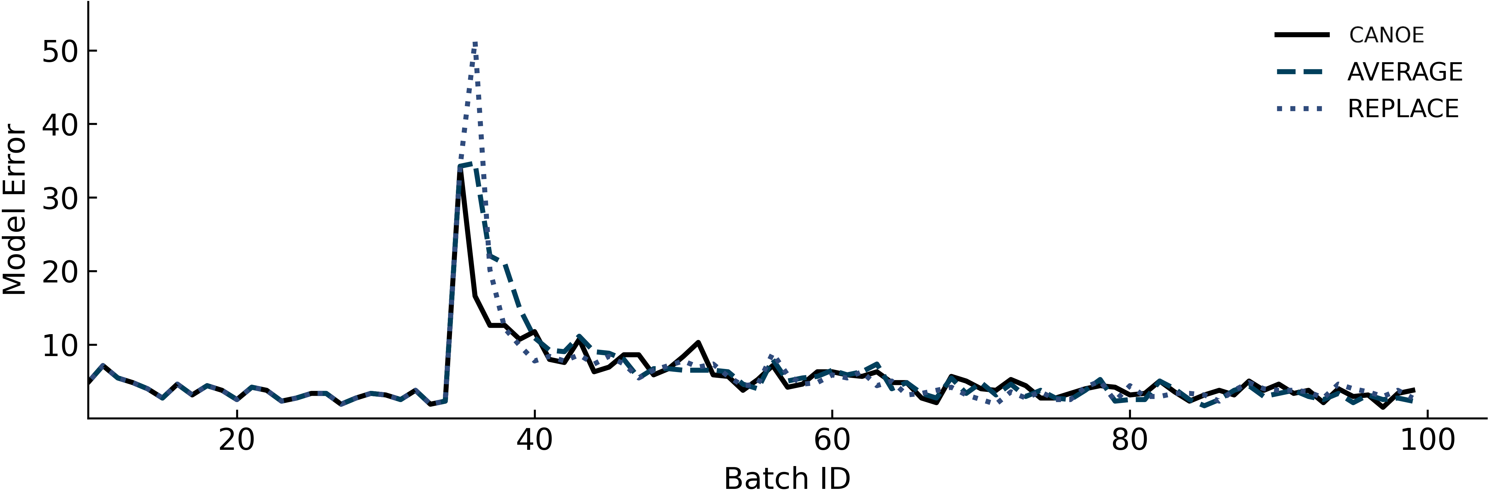
(a) Non overlapping workload

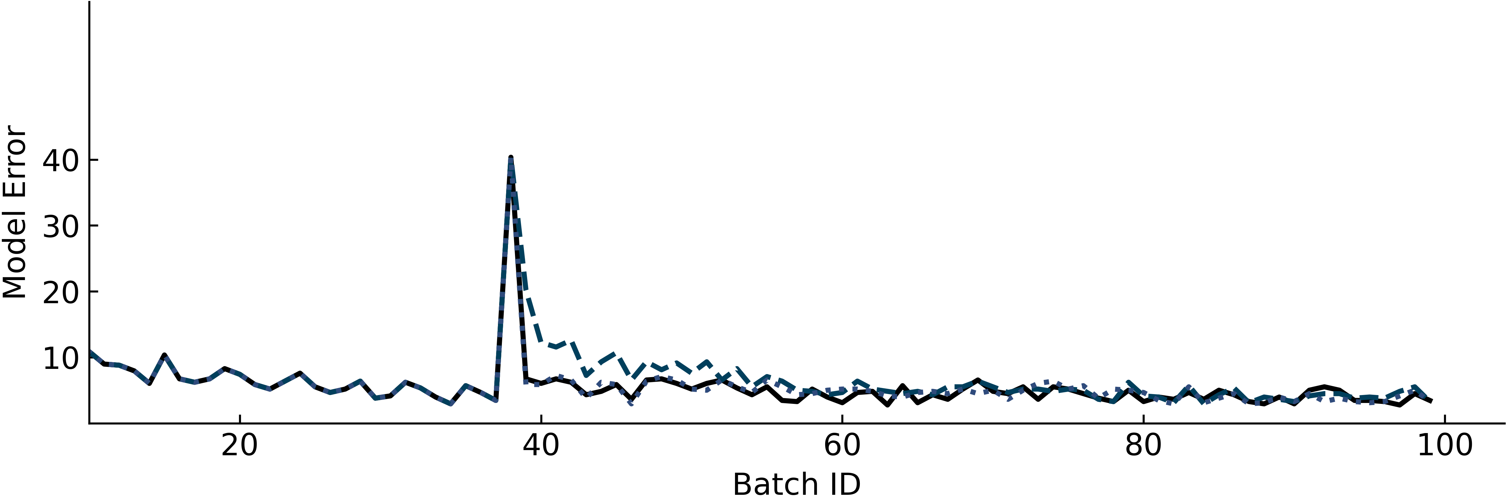
(b) Overlapping workload

Figure 2. Multi-model approach compared with averaging or replacing the existing model parameters: Canoe performed well and was consistent in both the scenarios; replacing the parameters worked well with overlapping classes and average performed better when the classes at the two nodes were non-overlapping.

To address the challenge C2, Canoe provides support for creating and managing helper models used for boosting the model at the target node.

After receiving the significant parameters from the helper node(s), the target node needs a mechanism to apply these updates to improve the predictive performance of its model. Let $W^{t}$ and $W^{s}$ represents the target node and significant parameters, respectively. A simple approach would be to apply the received knowledge directly on the existing target model. Different from replacing the significant parameters is to create the model by averaging the weights of target model with the received significant parameters. This technique would be similar to Federated average algorithm (McMahan et al., 2017).

The outcome of replacing or averaging the existing parameters is dependent on the workload distribution. Figure 2 illustrates the model error rate observed over the 100 request batches from a subset of the classes in the EMNIST (Cohen et al., 2017) dataset at the target node using the MobileNet (Howard et al., 2017) convolution neural nets for image classification. The workload distribution observed at different nodes in the system can vary. It can be overlapping where the workload observed at the target is a subset of the workload observed at another node, or non-overlapping where no two classes observed at the nodes are the same. To illustrate the impact of replacing or averaging the existing parameters we use two workloads – overlapping and non-overlapping. At batch id 35 a new class(es) is introduced at the target node. When the target node workload distribution is a subset of the workload observed at the helper node (overlapping), replacing the parameters would provide more benefits. However, when the workloads differ (non-overlapping), averaging the parameters would help more when compared to parameter replacement. Figure 2(a) illustrates that for a non-overlapping workload replacing the parameters further increases the model error rate since it replaces parameters for classes already learned by the model. When the target and helper model observe a similar workload, Figure 2(b) shows that replacing the parameters helps, whereas averaging the parameters would result in the target model taking more time to adapt to the new changes.

Multi-model approach. To decouple the way the significant parameters are used to update the target node’s model from the dependence on how the workload is distributed across the target and helper node(s) in the system, we use the significant parameters to create a helper model.

The existing model at the target node is well trained to predict the already observed classes, while the significant parameters received from the helper can assist in improving the prediction of the newly observed classes. As neither the target model nor the significant parameters can solely make accurate prediction, Canoe uses a multi-model approach where a helper model is created using a boosting technique (Dai et al., 2007; Freund and Schapire, 1997). Boosting converts or combines weak learners to form a strong the helper model. We use the original target model with the goal of maintaining the accuracy of the model for the existing classes. We use the helper model to provide a boost in accuracy for new classes which were already known at the helper node. The final output is a resultant of combining the output from both the models.

Helper model creation. As the target node receives only a subset of the parameters from the helper node(s), we consider two ways to create a helper model. In the first method, shown as Canoe (ZERO) in Figure 3, the helper model is created by using the significant parameters, and the remaining parameters of the model are set to $0$. Using $W^{h}$ to denote the parameters of the helper model, we formulate this as

(2) $$W^{h}_{i}\leftarrow\begin{cases}W_{i}^{s},\quad&\textmd{if $W_{i}^{s}$ is significant}\\ 0,&\textmd{if $W_{i}^{s}$ is not significant}\end{cases}$$

Neural network consists of interconnected neurons where each connection is associated with a weight which helps in determining the output. By having some weights in the layer as $0$ effectively reduces the magnitude of the output of that layer, eventually impacting the overall output. In the worst case, if the parameters in one of the layers are all set to $0$, all intermediate values and final class output scores would be the same for any input. In such a case, no useful information could be derived from the helper model output. Therefore, we consider a second method, which creates a helper model by combining the significant parameters from the helper node with the existing parameters from the target node. The resulting boosted helper model is represented as shown in Equation 3, and illustrated as Canoe (BOOST) in Figure 3.

(3) $$W^{h}_{i}\leftarrow\begin{cases}W_{i}^{s},\quad&\textmd{if $W_{i}^{s}$ is significant}\\ W_{i}^{t},&\textmd{if $W_{i}^{s}$ is not significant}\end{cases}$$

Boosted model output. After creating the helper model we update the prediction function to take into account the classification outputs from the helper model. At this stage we have a target model, good for the existing classes, and a helper model, good for the new ones. We use average of both the models to compute the final output, though other functions can be plugged in.

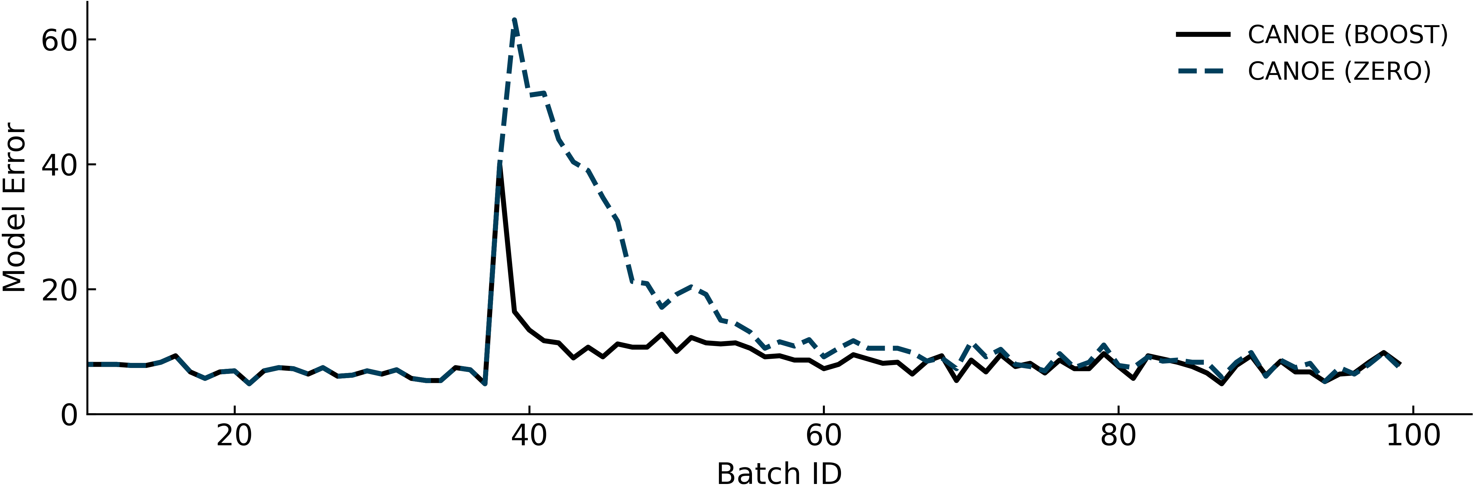
Figure 3. Boosted model error rate for two types of helper models. Helper model created with boosting from target model performs better than the one created only using the significant parameters.

Figure 3 compares the two approaches of helper model creation, and shows that a helper model created using the target model is more effective when compared to the one created using no prior information: Canoe (BOOST) experiences a lower spike in the model error rate when a previously known class is observed at the target, and it more quickly adapts and converges to its original accuracy.

Managing helper model chains. The use of helper models improves the overall performance of the model, however, it creates the problem of repeatedly generating new helper models, on-demand, whenever a concept drift is detected. Maintaining an ever lasting chain of helper models would add more strain on the resources at the edge node. To alleviate this pressure we take two steps. First, since the goal of the helper model is to provide assistance to the target model, we freeze the helper model by not retraining it, while we continue to (re)train the target model. Second, we discard the helper model(s) as the performance of the model stabilizes for the class(es) for which the helper model was created.

A straightforward way would be to discard the model after a user-defined number of batches. Discarding a helper model prematurely could result in a second smaller drift, while discarding it too late would result in additional unnecessary computation and resource usage. To avoid this uncertainty Canoe uses a dynamic approach where after every request batch the performance of the target model is tracked separately and is compared to the pre-drift performance. When the target model reaches the earlier performance level the helper model is discarded. In presence of chain of helper models Canoe provides an additional check which compares the predictive performance of the new classes for past $L$ batches to determine which model to discard. The precise value of $L$ depends on the number of samples observed, models and dataset. For our experiments the value was experimentally determined and we leave the online tuning of $L$ as a topic for future work. The precise discard policy is configurable.

6. Canoe Runtime

We describe the interaction among the different components in Canoe, and discuss the requirements for its implementation in the context of existing ML frameworks.

Canoe Components. The runtime is divided into three main blocks – ML Model Interface (ML), Knowledge Transfer (KT), and Collaborative Component (CC), shown in Figure 4.

The CC component controls how a node collaborates with other nodes in the distributed system. It encapsulates the functionality needed to discover a helper node and to determine when to reach out for help. Synchronizer is responsible for exchange of metadata that provides the necessary state for helper node discovery. Drift detector determines when interactions with a helper node get triggered, ideally, when the local model degrades in performance, based on a drift detection algorithm, as in (Daga et al., 2019). In (Lu et al., 2019), synchronization is performed periodically, and is always coupled with a receiving help via model distillation.

The ML component provides the interface to the machine learning framework (e.g., PyTorch or TensorFlow). It uses the predict interface to perform the prediction on the incoming request data batch. The output of the prediction is passed to an operator component. During normal operation, the prediction result is used directly. In the presence of helper model(s), during periods of knowledge transfer, the operator averages the outcome of all the model(s). The cycle is completed with training the resident target model with the new batch of data using the (re)train interface.

The KT component facilitates the knowledge transfer mechanisms. At each node, parameter picker supports the parameter selection mechanism, and is invoked asynchronously, when a node receives a request for help for a specific class(es). The process is performed by either the continuous or the on-demand mechanism. The resulting parameters are sent to the target node where booster creates a new helper model. When helper model(s) are created, the operator function is adjusted to perform averaging, and a discard checker monitors the convergence process to determine when helpers are to be discarded, dynamically or statically after predefined number of batches, according to a configurable policy.

Canoe exposes APIs to configure the system parameters controlling the knowledge transfer process in terms of the percentage of significant parameter transferred from the helper, the number of request batches to be locally stored for on-demand parameter selection, the discard policy, etc. In this manner, Canoe exposes new tuning knobs that control the knowledge transfer process in terms of its effectiveness in improving the target model and the overheads it introduces, which can be used for new types of resource orchestrators for distributed learning.

Implementation. We implemented a prototype of Canoe for the PyTorch and TensorFlow ML frameworks, using Flask to provide support for communication among different nodes.

The use of the different frameworks exposes the following requirement for implementing Canoe. The significant parameter selection can be done in different ways, however using the dynamic selection approach would require the ML framework to provide corresponding APIs for calculating the gradients on the model. The framework should also provide the capability to dynamically create, use and discard helper model(s), in conjunction with the existing model. Given the available APIs in PyTorch, our implementation of Canoe supports all the mechanisms described in §5. TensorFlow creates a static computation graph before a model is run and any interaction with the model is tightly integrated with the session interfaces and state placeholders. Due to these limitations, TensorFlow cannot support on-demand significant parameter selection, hence, this implementation of Canoe uses the continuous significant parameter mechanism. Additionally, since TensorFlow does not permit models to be dynamically created, we use a pool of helper models from the initial state of the experiment. The resulting TensorFlow implementation of Canoe introduces runtime memory overheads which may be prohibitive for practical settings. We note that the limitations of the current TensorFlow APIs may be addressed in future versions of the system, and we still compare the two implementations to illustrate the generality of Canoe for realizing knowledge transfer across models developed with different ML frameworks (§7.5).

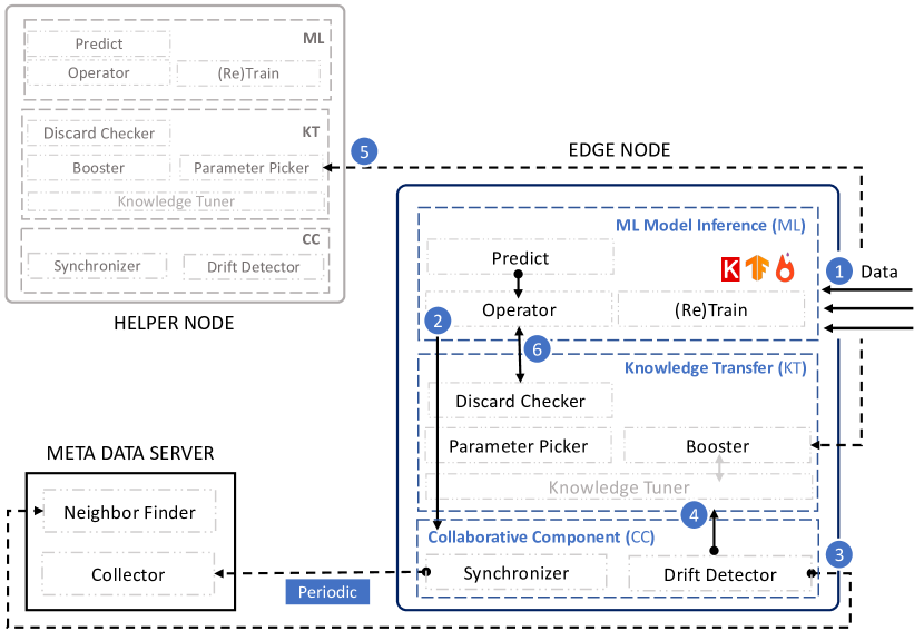
Figure 4. Canoe System Components.

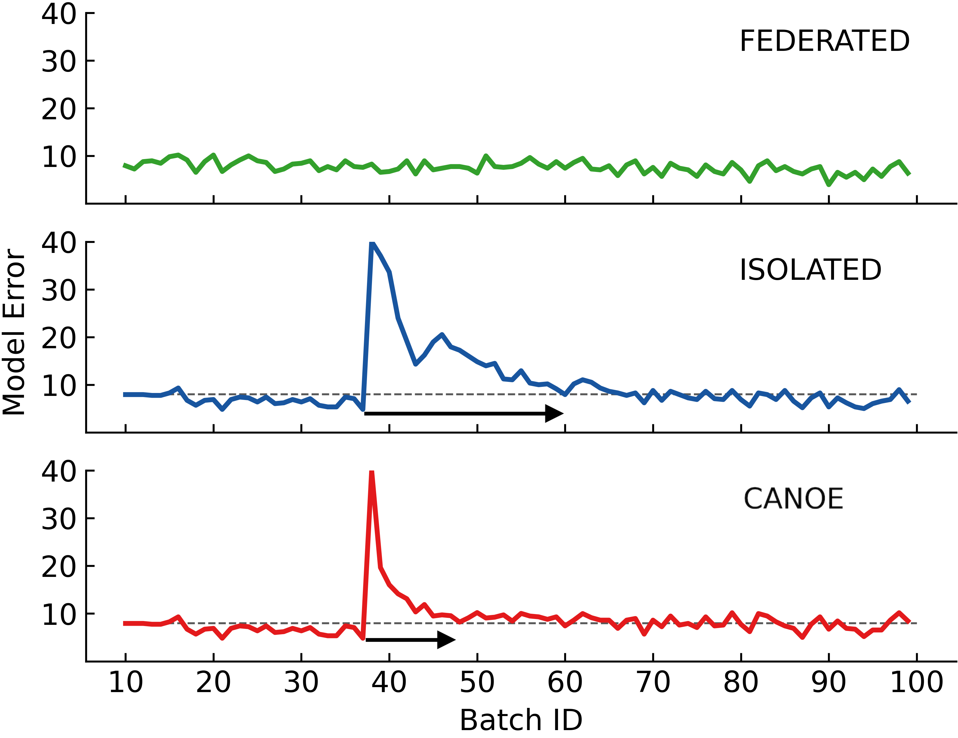
(a) MobileNet

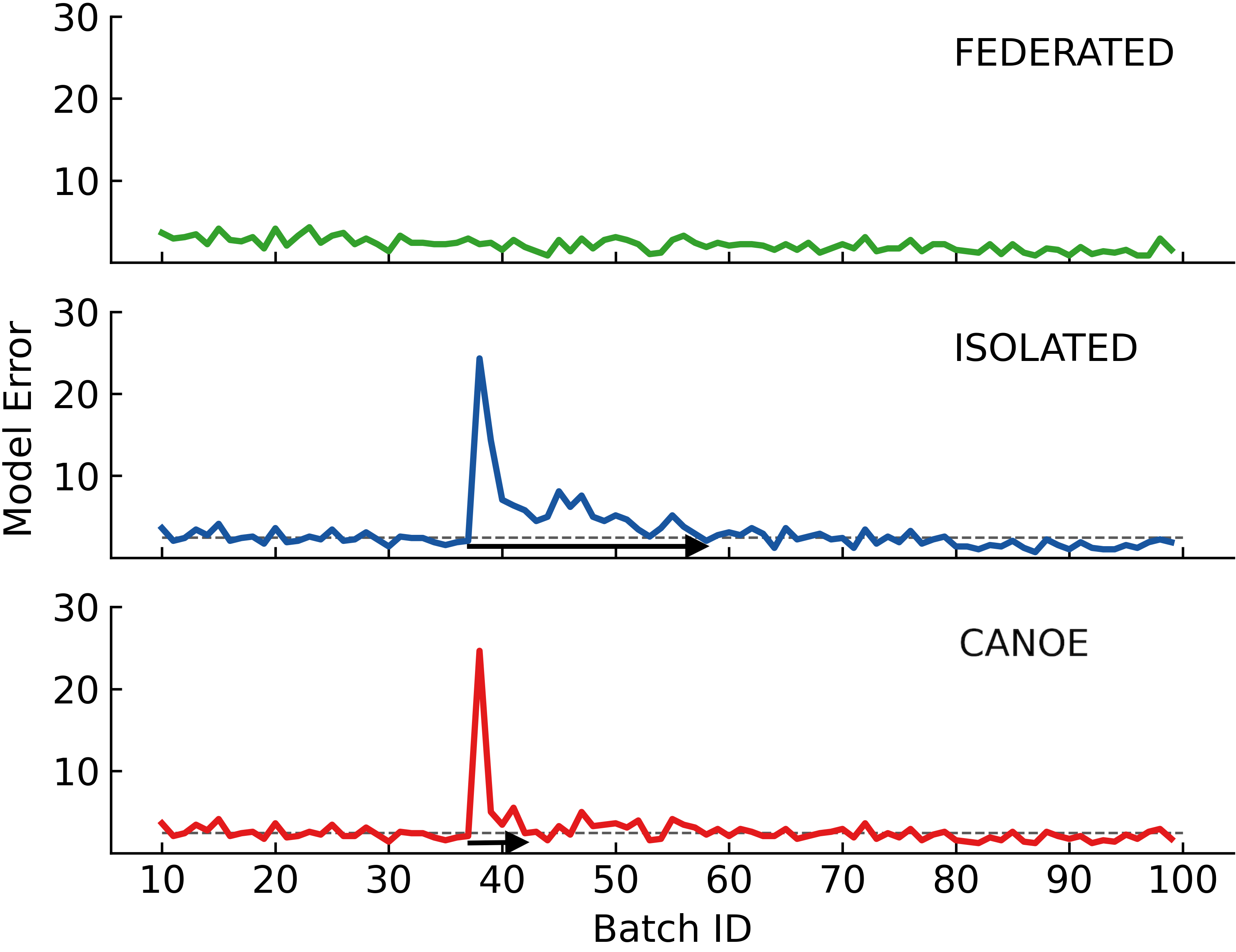
(b) DenseNet

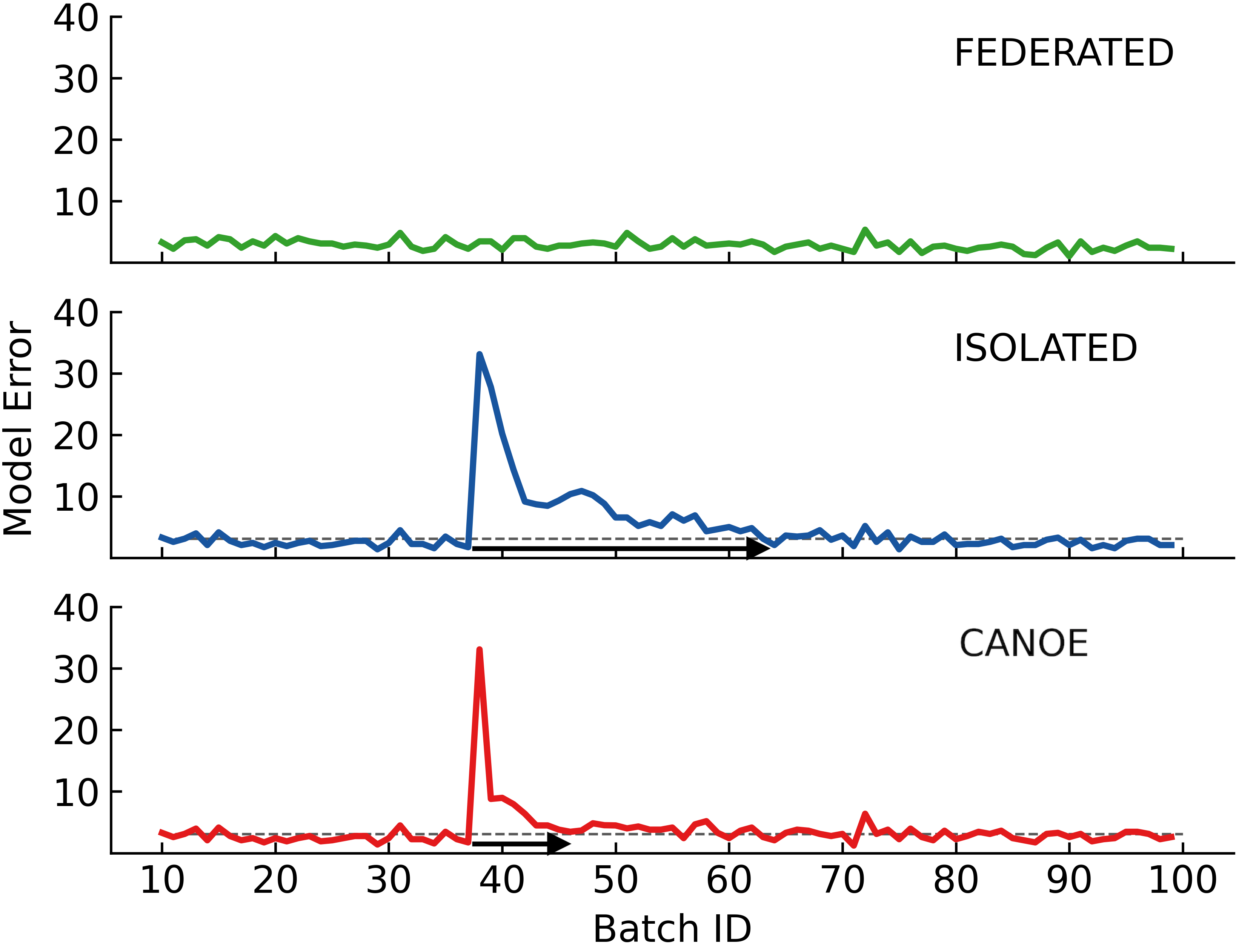
(c) ResNet

Figure 5. Performance comparison for introduction workload distribution (lower error rate is better) showcasing overall model error change. Misclassification of introductory class degrades the model performance. Canoe is able to quickly adapt to the change in distribution (given by the horizontal arrow). The horizontal dotted line (in black) defines the lower bound obtained through an offline training.

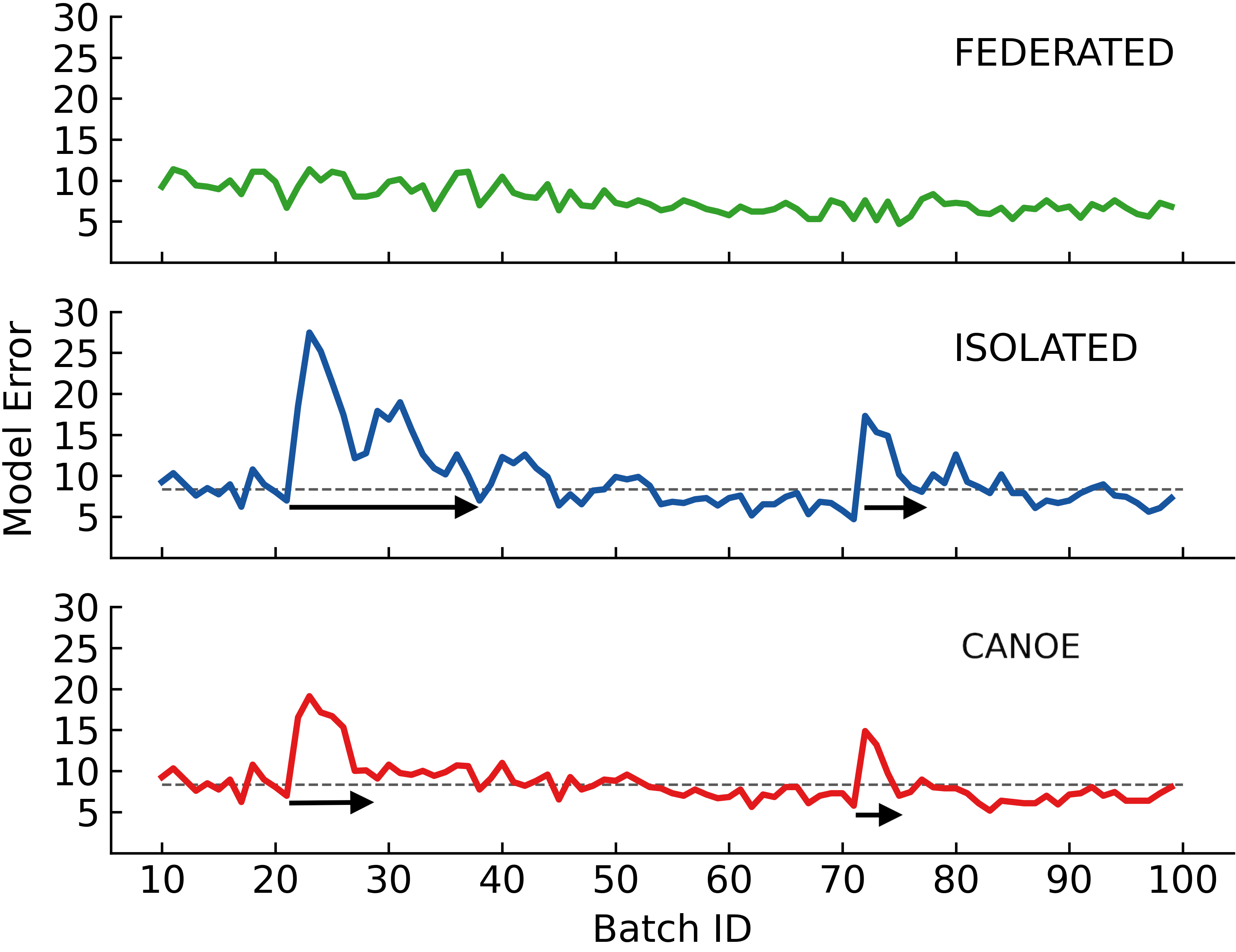
(a) MobileNet

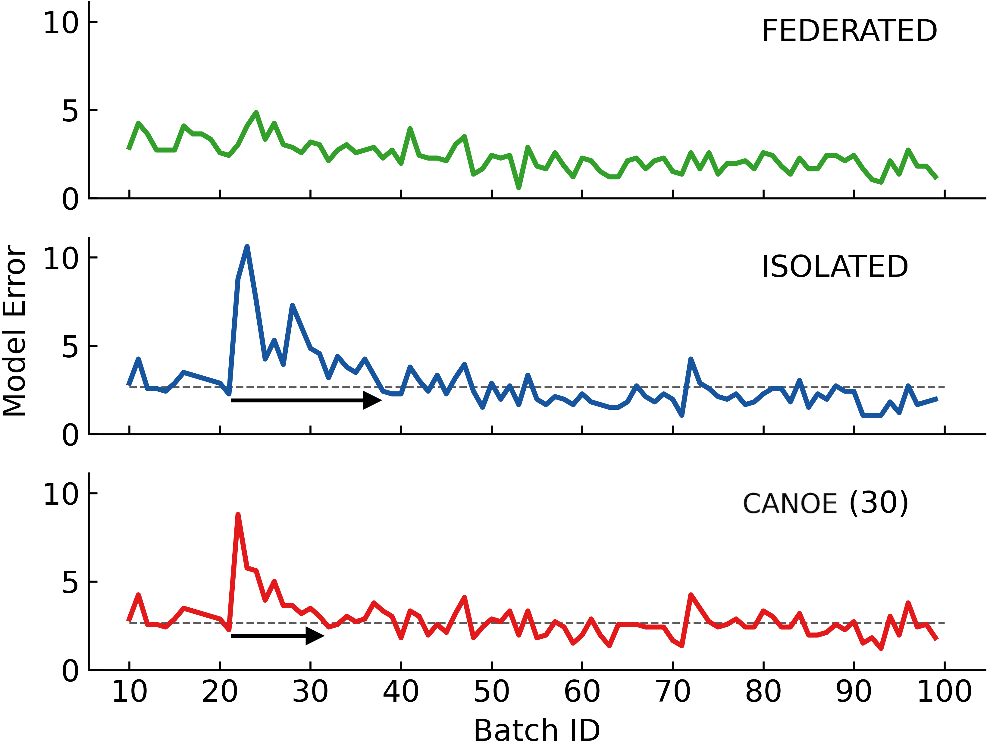
(b) DenseNet

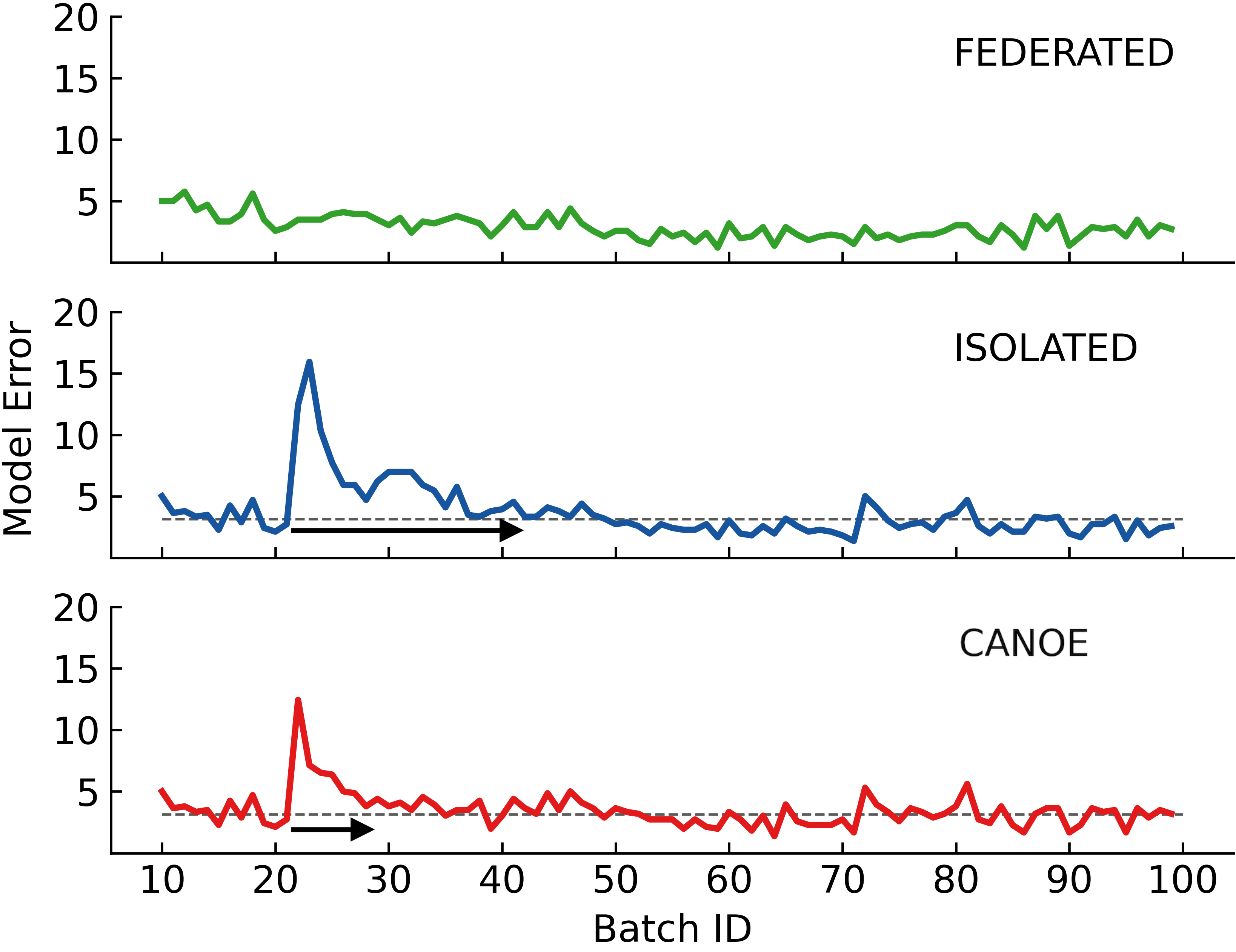
(c) ResNet

Figure 6. Performance comparison for fluctuation workload. Similar to Figure 6 Canoe is able to adapt to the changes in the distribution and behaves close to a federated learning system.

7. Evaluation

The evaluation of Canoe explores the following questions:

• How effective is the knowledge transfer mechanism enabled by Canoe in allowing neural network models to adapt to change, and what impact does it have on improving the overall model performance and curtailing data transfer costs? (§7.2)

• What are the overheads introduced by the parameter selection in Canoe on the helper nodes, and by multi-model learning on the target node? (§7.3)

• What is the impact of the different system-level parameters in Canoe on the overall benefits? (§7.4)

We used multiple workloads, models, and frameworks, as described below, to ensure the generality of the observations.

7.1. Experimental Methodology

Experimental Setup. We evaluate Canoe on a cluster of 5 nodes on the Chameleon Cloud (Mambretti et al., 2015) experimental platform. All nodes are Intel(R) Xeon(R) 125GiB RAM with 48 cores running 2 threads per core at 2.30GHz. The experiments are performed with two versions of Canoe, integrated with two existing machine learning frameworks: PyTorch v1.7.1 and TensorFlow v2.3.1 (§7.5).

Applications, Datasets, Workloads. We use two application use cases in the evaluation: image classification and intrusion detection (§7.6).

For the image classification use case the results are obtained with the EMNIST dataset (Cohen et al., 2017), consisting of 280k data samples. We made similar observations with the smaller MNIST dataset (LeCun, 2010). These datasets are derived from the NIST Special Database 19 (Grother, 1995) where EMNIST follows the same conversion paradigm used to create the MNIST dataset. The outcome is a set of datasets that constitute a more challenging classification tasks involving letters and digits, and that shares the same image structure and parameters as the original MNIST task, allowing for direct compatibility with all existing classifiers and systems.

For the intrusion detection use case, we used the NSL-KDD dataset (Tavallaee et al., 2009) which consists of benign network requests mixed with various malicious attacks consisting of 126k records. It is derived from the KDD’99 dataset (kdd, 1999) where redundant and duplicate records were removed to avoid bias in the learning process.

During the experiments, each edge node processes request batches over time, with each batch consisting of a varied number of data points corresponding to different classes in the dataset. To create a change in class priors that triggers the need for collaboration and knowledge transfer, we generate workloads with several synthetic request patterns, corresponding to introduction of a new class at an edge node, fluctuation, where a new class appears and disappears, with overlapping and non-overlapping classes, as described in §5.2. The use of synthetic workload patterns is due to the limited availability of real infrastructure and data with both temporal and spatial metadata on the request distribution. The concrete patterns we use are based on information about distributions used in other research (Daga et al., 2019; Polese et al., 2018; Paul et al., 2011b; Zhou et al., 2012b). The extensive nature of the experiments successfully demonstrates the benefits achieved from the mechanisms provided in Canoe.

Models. For the image classification use case, most of the presented results are based on PyTorch and the MobileNet (Howard et al., 2017), DenseNet (Huang et al., 2018) and ResNet (He et al., 2015) CNN models. The models are fine tuned using 2k data points from the EMNIST dataset using Adam optimizer and learning rate 0.00005, and trained for 20 epochs with batch size of 30. Their sizes and parameter counts are summarized in Table 1. We also used the MobileNet, DenseNet and InceptionNet (Szegedy et al., 2014) models provided by TensorFlow v2.3.1, to confirm the effectiveness of Canoe across different machine learning frameworks (§7.5).

The intrusion detection use case uses a four-layer DNN model with 209k parameters, as described in (Gao et al., 2020). For model initialization we used the SGD optimization algorithm with a learning rate is 0.000005 and 25k data points. The model is trained for 20 epochs with batch size of 30.

Metrics. When using local, tailored models, as is the case in isolated or collaborative learning, a change in the workload pattern at a node via the appearance of previously unseen classes, results in a temporary drop in the predictive performance of the model, observed as an increase in its error rate. The time taken for the model to reach back the acceptable performance levels is defined as the model’s adaptability to change. Models using FL are usually impervious to such changes, because the frequent model update from the aggregator node in the FL framework continuously distributes the knowledge obtained at one node to all the other nodes in the system. In isolated learning, no knowledge is received from any other node in the system, instead the model performance ultimately improves as a result of the online learning (retraining) on the data from the incoming request batches. The goal of Canoe is to improve the model’s adaptability by minimizing the time required to adapt to change compared to learning in isolation, while also reducing the data transfer requirements compared to federated learning.

We evaluate Canoe by measuring the improvements in adaptability to change it offers compared to isolated learning. Given the synthetic nature of the workloads, we measure time in terms of the number of batches that need to be processed for the model performance to reach the same error rate as what is possible with FL. We also measure the improvements that Canoe provides in terms of per-node and aggregate data transfer costs (in bytes). Finally we measure the runtime overheads of Canoe in terms of additional compute (using processing time as a measure) and memory resources.

7.2. Benefits of Canoe

Table 1. Raw data transferred (MB) and gains per update per node in FL vs. Canoe. In Federated Learning data is transferred to send and received model update while in Canoe data is transferred to share metadata information and during knowledge transfer.

CNN Model	Million Parameters	Federated Learning		Canoe		Data Transfer Gains
		Out	In	KT (In)	MdS (Out)	No Drift ($\times$)	With Drift ($\times$)
MobileNet	3.54	6.38	7.36	4.57	0.00058	23684	3
DenseNet	8.06	16.18	18.35	8.80	0.00058	59507	4
ResNet	11.69	12.19	13.75	8.55	0.00058	44713	3

Table 2. Ratio of total data transferred (in and out) of a node in Federated Learning versus Canoe for a 5 node setup for an entire experiment consisting of 100 request batch.

Model	Workload	Aggregator($\times$)	Member($\times$)
MobileNet	Introduction	1062	267
	Fluctuation	644	161
DenseNet	Introduction	1897	350
	Fluctuation	1396	346
ResNet	Introduction	1078	271
	Fluctuation	1069	268

Adaptability to Change. Figures 5 and 6 illustrate the adaptability enabled by Canoe for the introduction and fluctuation workloads where the system uses $50\%$, $20\%$ and $30\%$ of the significant parameters for MobileNet, DenseNet and ResNet, respectively. The parameter $Z$ that controls the percentage of knowledge transferred for each of the three models is experimentally chosen to that it minimizes data transfer while keeping the model adaptability within 10% of the best case. For the given testbed configurations, in these experiments the helper model is created after within 4 request batches after the drift detection. We observe that with Canoe, the models converge to the performance level equivalent to using a global model up to $2$ to $3.5\times$ faster as compared to an isolated system. For the fluctuation workload and MobileNet, in Figure 6(a) we observe a second spike in the model performance as the class reappears in the later part, while for DenseNet and ResNet we do not observe any change for the same workload. This is because the other two models are larger and are able to retain more information even when the class was not present for few request batches.

Reduction in data transfer costs. The collaborative learning technique used by Canoe works on the curve of finding a tradeoff at spending few cycles to adapt to the change in the workload versus the data transfer cost associated in regularly creating and updating a global model, as done in FL. We summarize these costs in Table 1. In FL, for each update period, for a member node the data transfer cost consists of the delta in the local model since the last batch (Out) and the received aggregated model update (In). For Canoe, the per-update data transfer cost at each node consists of the metadata sent to the MdS server (MdS(Out)). When data drift is detected on a node, that node also incurs the knowledge transfer cost (KT). For neural networks, the change in a local model ($Out$) or aggregated model updates ($In$) are significantly larger when compared to the metadata (few kBs) used by Canoe, and this leads to drastic reductions in the data transfer costs, compared to FL, up to $10^{4}\times$, as seen from the table. Moreover, since only a fraction of model parameters are transferred as part of knowledge transfer in Canoe, this too could result in data saving of up to $4\times$ when compared to a single model update request in FL.

In Table 2, we compare the total data transfer for the same experiment with 5 edge nodes with FL and Canoe as used in Figures 5 and 6. As the collaborative approach requires model data to be exchanged only when there is a drift in the model performance at a target node, while in FL all nodes frequently receive model update across the system the outcome is an overall data transfer reduction of 2-3 orders of magnitude, depending on the the workload and model.

7.3. Cost of Canoe Mechanisms

Extracting significant parameters. Using Canoe to perform knowledge transfer introduces runtime overheads associated with the execution of the necessary mechanisms. We present these costs in the context of the same experiments as above using the introductory workload.

The continuous method for parameter selection stores the sensitivity value of all parameters for all of the classes, and its overheads depend on the number of layers and parameters of the model. For our dataset and given models, this introduces additional memory overhead of $140MB$, $320MB$, $470MB$ for MobileNet, DenseNet and ResNet, respectively. The on-demand approach creates a local datastore which is only used when a request from a target node is received. For our dataset, with an average of 600 data points in a request batch, storing only the most recent request batch was sufficient and required an addition of $6.8MB$ of memory. We performed the same experiments for different batch sizes, starting from as low as 50 data points, and, across workloads, observed similar gains in the overall benefits of Canoe, with expected reduction in the runtime overheads.

In terms of the compute overhead, the on demand approach adds an overhead in the response time of $0.9$ to $1.35\times$ the time required to process a request batch. The continuous approach by pre-calculating these values avoids such delays in the critical path of response, however, adds an overhead of up to $0.7\times$ the time required to process a request batch, for every request, as shown in Table 3.

Table 3. Overhead in performing mechanisms described in Section 5 normalized with the time required to process a request batch.

Model	Continuous ($\times$) per batch	On-Demand ($\times$) per request	Helper Model ($\times$)
MobileNet	0.70	0.98	0.08
DenseNet	0.65	1.35	0.11
ResNet	0.70	0.95	0.14

Helper model creation. The time taken to create the model depends on the size of the portion of model transferred from the helper node, as shown in Table 1, and the time taken to create a model at the target node. Upon receiving the significant parameters creating a helper model takes only up to $0.14\times$ the time required to process a request batch.

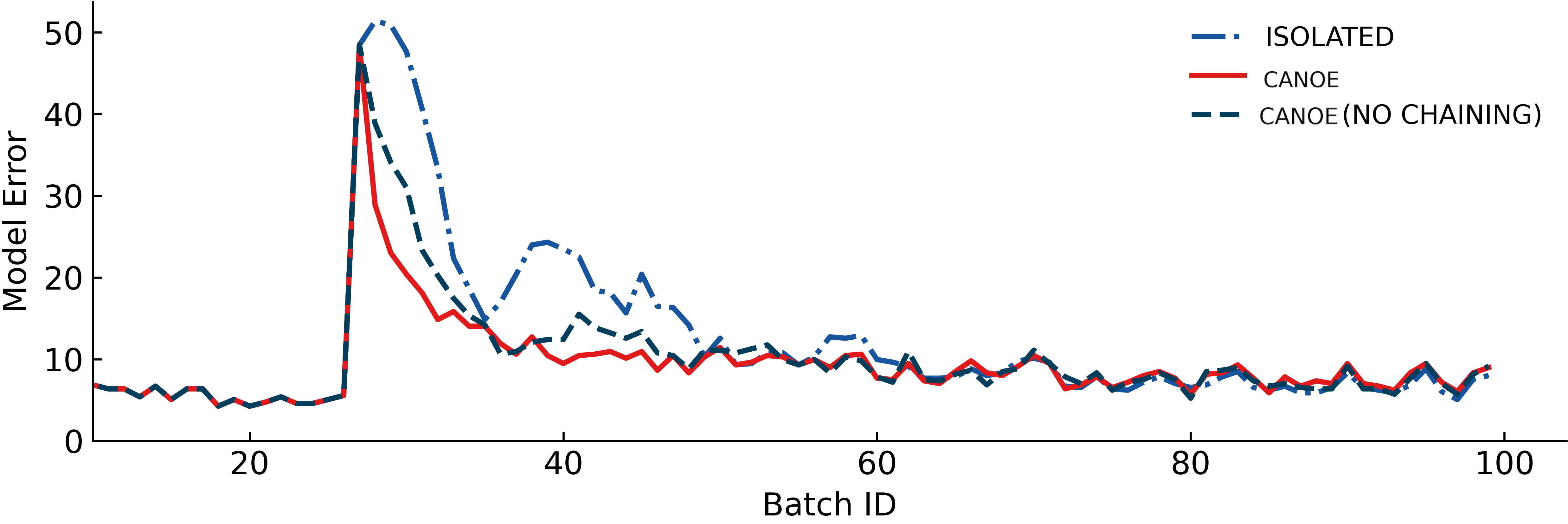
Figure 7. Chain of helper models improves the predictive performance and helps the system adapt to the new changes faster.

Management of helper models. A helper model in Canoe uses similar memory as the resident node model however since the model is frozen, no additional resources are required after its creation. Using multiple helper models in a chain adds to the memory overheads. Thus, if the knowledge about the introductory classes at the target node is dispersed among multiple nodes, in such a case Canoe exposes a tradeoff of using more memory for a short duration of time by deploying chains of models vs. spending more time in adapting to the changes. Figure 7 shows the collaborative performance of using help from only one of the nodes (no chaining) compared to creating chain of models from multiple nodes. The ability to combine multiple knowledge sources in Canoe provides the lower bound on adaptability to the new changes in the system.

7.4. Sensitivity Analysis & Opportunities

The benefits of Canoe are coupled with the quantity and quality of knowledge transferred. We analyze this by considering the performance of the models and workloads evaluated in §7.2, and varying the amount of knowledge transferred and the quality of the helper node used for knowledge transfer.

Impact of quantity of knowledge transferred. Canoe controls the portions of the significant parameters that are transferred via the parameter $Z$. We evaluate the impact of different values of $Z$ on the model’s adaptability and data transfer costs. Figure 8(a) shows the results of evaluation for introductory workload pattern for MobileNet; the results with the remaining models had a lower sensitivity to $Z$ than what we present for MobileNet. The results illustrate two important aspects of Canoe. An effective helper model can be created using only a portion of the relevant parameters. The percent of significant parameters received from the helper node have a direct impact on improving the target node’s overall predictive performance and reduction the data transfer cost. The higher value of $Z$ (90) may provide improvements in error rate, when compared to $Z$ (10), specifically for this setup 25% reduction in average model error rate while using the helper model. However, it would result in $5.53\times$ more data transfer.

We note that Canoe introduces new ability to control a tradeoff among learning performance and data transfer costs, by using the amount of knowledge that should be transferred across nodes as a configuration knob. This can be leveraged by future learning management policies to adapt the effectiveness of the process based on the model used and the deployment scenario.

Impact of quality of helper node. As discussed in §2 a helper node can be identified from the model and node metadata, however, its choice can have an impact on the collaborative learning process. To understand this, in Figure 8(b), we compare the execution of Canoe and Z(50) with MobileNet and the same helper node as used in the previous experiment, to that of two other scenarios where the helper nodes have observed only 50% (L50) and 10% (L10) of the data observed in the baseline. As expected, we observe that the quality of the helper node does impact the realized benefits from Canoe. However, we see that using even a weaker helper node (L10) can still be useful, compared to just learning in isolation. Note that, simply increasing $Z$ for a weak helper node would not be helpful, as the quality of the model parameters is not good for the required knowledge.

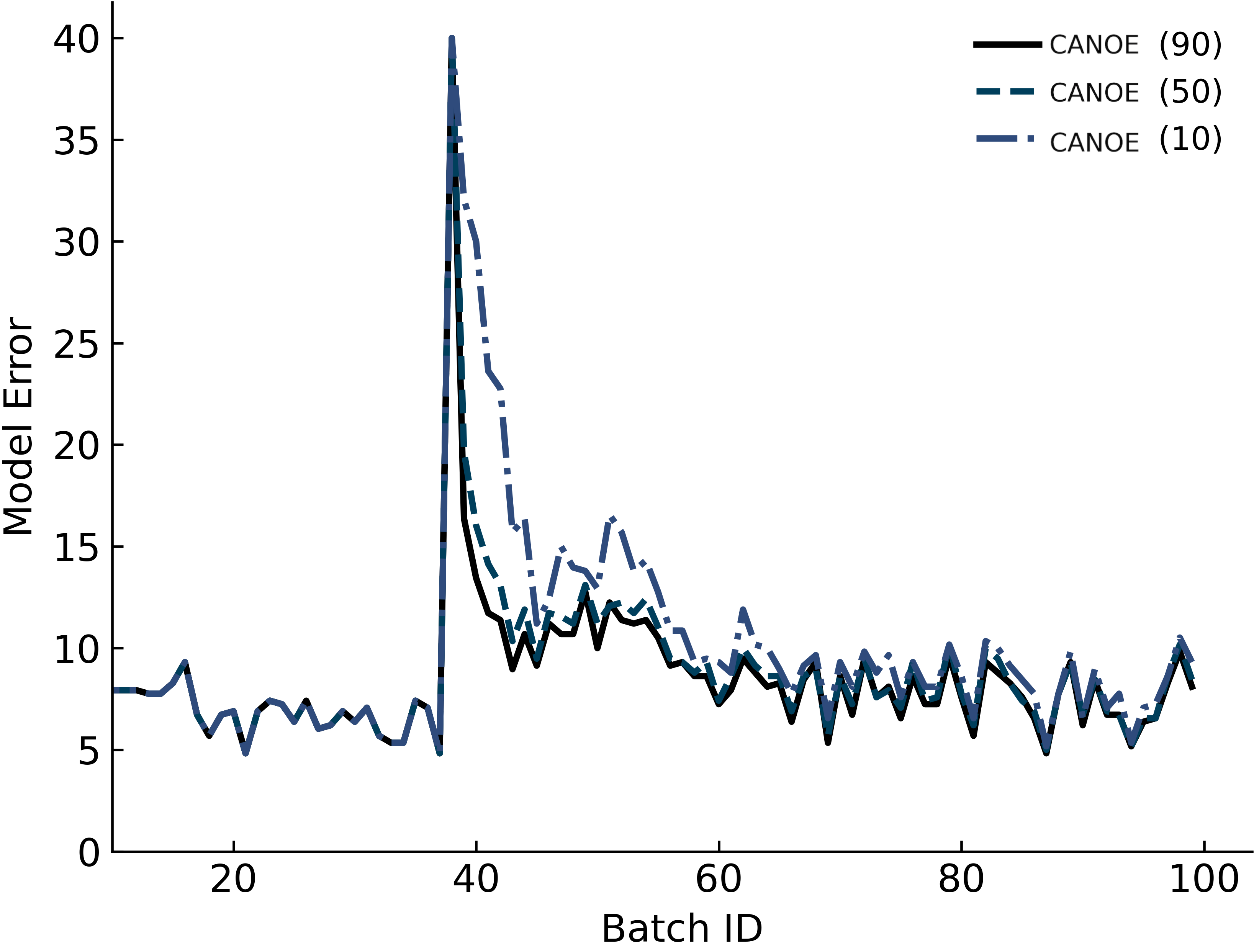
(a) Significant parameter selection

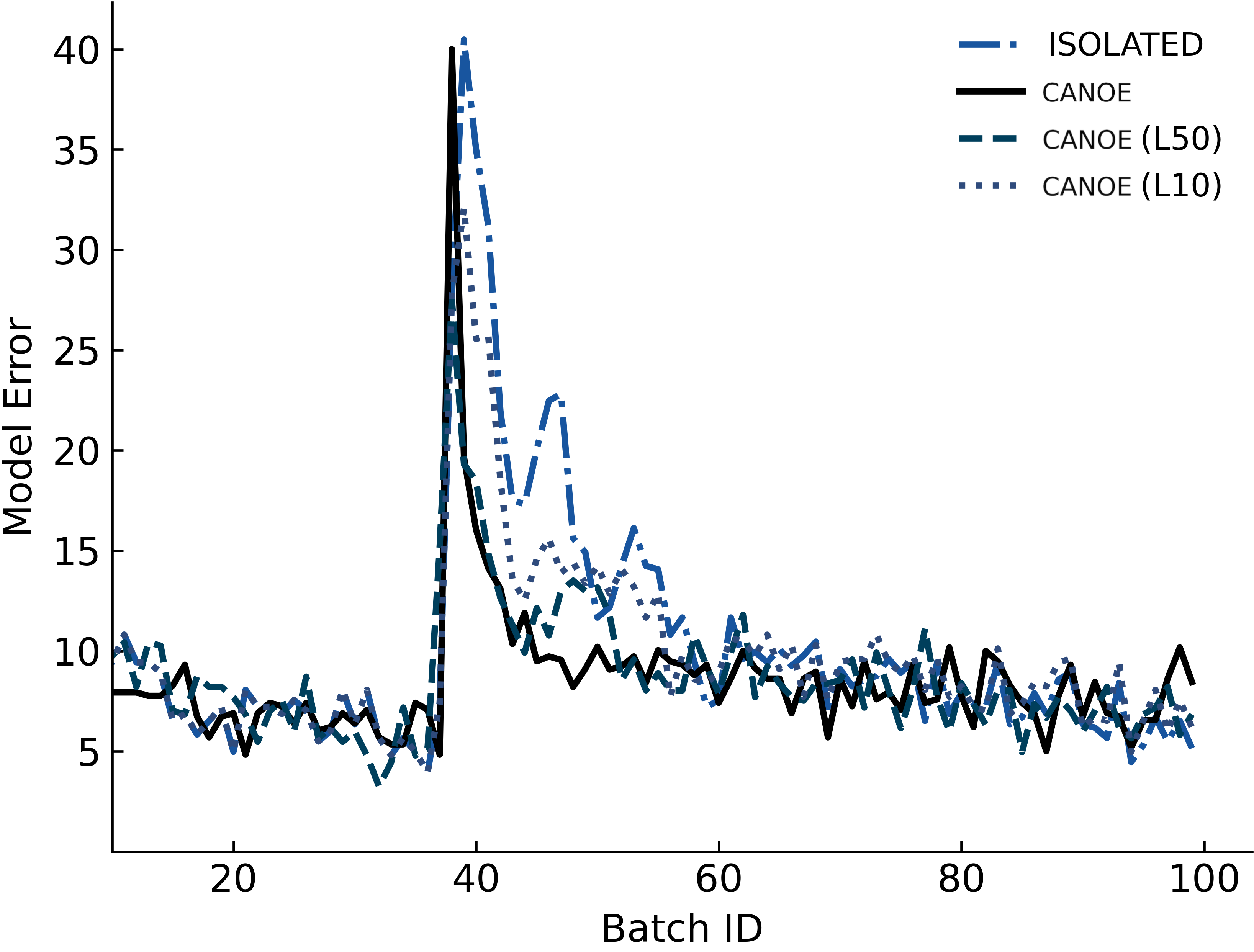
(b) Helper node quality

Figure 8. Comparison of impact of percent of significant parameter $Z$ (left) and impact of quality of helper node model (right).

7.5. Extensibility to Different ML Frameworks

To demonstrate the generality of the system, Canoe is implemented for PyTorch (PT) and TensorFlow (TF). With TF, Canoe creates a pool of helper models from the initial start of the learning process, which are later updated using the significant parameters received from the helper node. Parameter sensitivity values are computed using the continuous technique. Due to these limitations, and for brevity, the earlier section presents the results from PT only. Based on experiments with the introduction and fluctuation workloads used with the PT evaluation, and the MobileNet, DenseNet and InceptionNet CNNs, Canoe adapts to change up to 3$\times$ faster than isolated learning, while using only $60\%$, $30\%$ and $30\%$ of the model respectively. This results in overall data transfer reduction of $700$ to $1200\times$ compared to using FL.

7.6. Use Case – Intrusion Detection

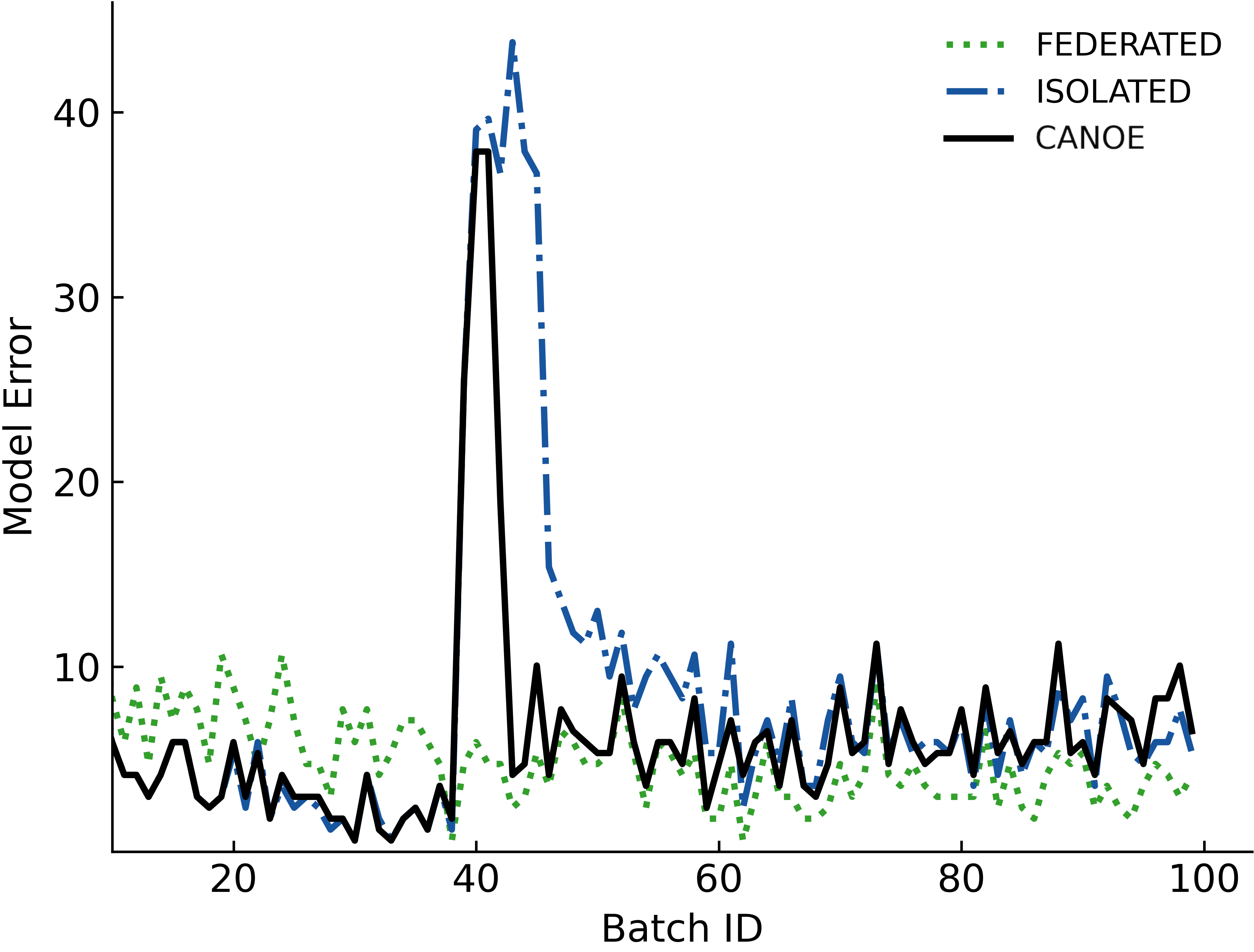
(a) Overall Error

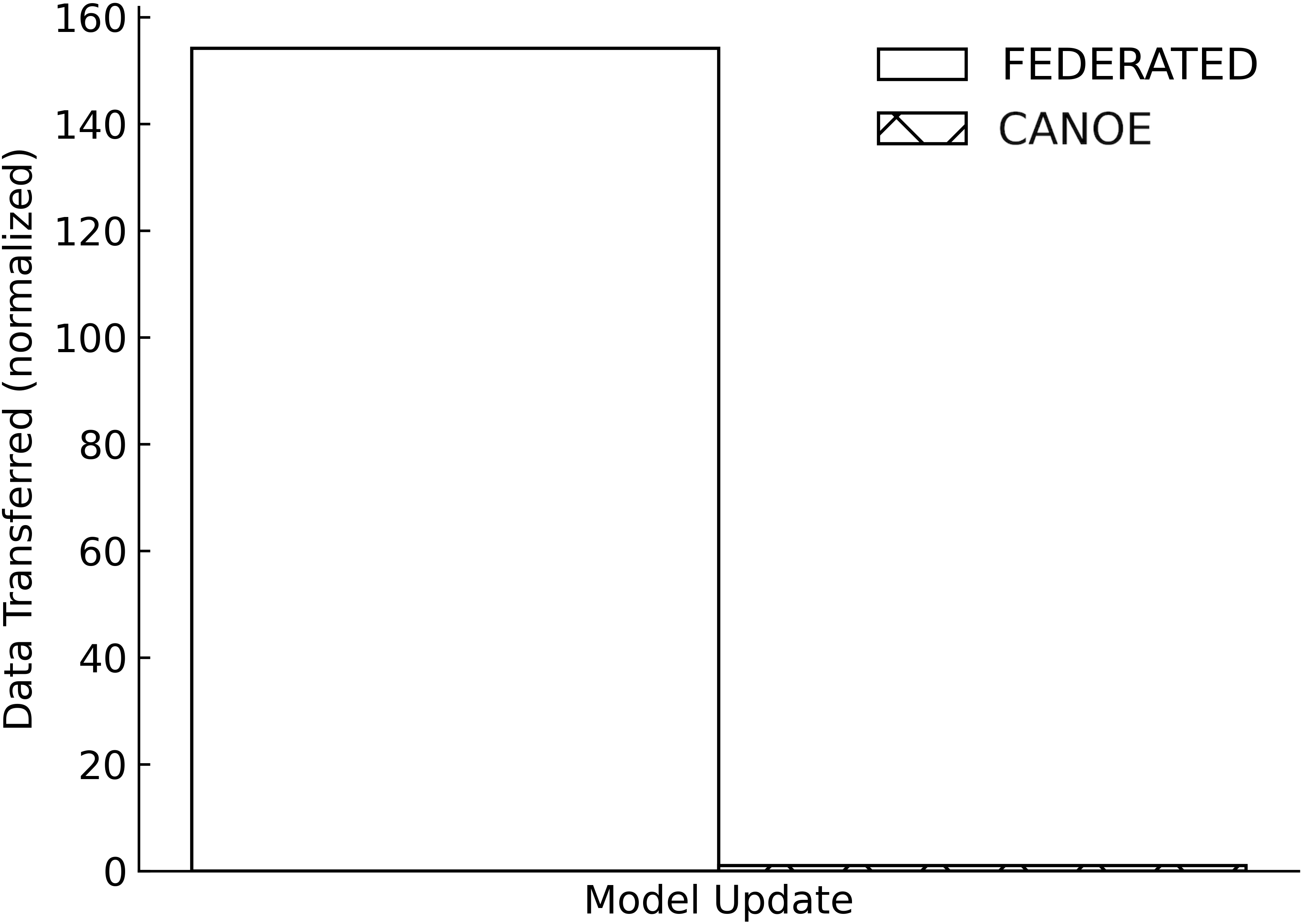
(b) Data Transfer

Figure 9. Performance and total data transfer comparison for network attack dataset using ORF to classify begin request against DDoS and port scan attack requests. Comparison of model performance and data transfer overhead for network attack dataset using introductory workload.

Intrusion Detection System monitor and analyze the network to detect anomalies and attacks. This use case is based on the NSL-KDD dataset (Tavallaee et al., 2009) which consists of four types of attacks: Denial of Service Attack (DoS), User to Root Attack (U2R), Remote to Local Attack (R2L), and Probing Attack (Probe). The testbed consists of 5 edge nodes, where initially the target node observes only the R2L and Probe attacks, while the other nodes experiences all of the attacks. After some time the target node starts to experience the DoS attack. We use a four layer Deep Neural Network model as described in §7.1 with introduction workload consisting of 100 request batches with $\sim$400 data points in each batch and $Z$(40).

Results. Figure 9(a) illustrates the model performance for FL, Canoe and isolated. FL allows the target node to classify the attack immediately, since the attack was observed by other nodes earlier, and is captured in the global model updates. In isolated learning mode, the target node experiences both a large spike in its model error rate, and takes substantial time (equivalent of 20 batches) to retrain its model to the original performance (error rate). Canoe bridges the gap between the above two system. The collaborative process helps the target node adapt to the new attack $1.75\times$ faster than isolated system and to provide similar average model error rate compared to federated learning system with $600\times$ less data transferred over the wire.

8. Related Work

Distributed Machine Learning. Since its introduction, Federated Learning has emerged as a go-to approach to distributed machine learning (Konečnỳ et al., 2016). Follow-on work (Konečnỳ et al., 2015; Arivazhagan et al., 2019; Bonawitz et al., 2017) has introduced a number of optimizations, including recent solutions which speed up the convergence and improve the accuracy through guided member node selection based on developer specified criteria, as done in Oort (Lai et al., 2020). Different from Canoe, FL approaches have a goal of learning a generic ML model that will be used by all nodes in the distributed system, which justifies the data transfer costs.

To address the data transfer overheads in geo-distributed systems, Gaia (Hsieh et al., 2017) distinguishes among communication over local (LAN) vs. wide area networks (WAN). Nodes within LAN use a strong consistency model as used in FL, but only significant model updates are shared among WANs to save communication and speed up training. The goal of identifying a significant model update in Gaia is orthogonal to that of identifying significant model parameters, as the former applies to the model overall, whereas the technique used in Canoe is concerned with identifying a portion of the model that most contributes to the model quality with respect to a specific class. As with FL, the goal of Gaia is to learn a global model, shared across the distributed system.

In contrast, collaborative distributed learning approaches described in §2, are developed for environments where a global model is not needed (Hong and Chandra, 2019; Lu et al., 2019; Daga et al., 2019; Anil et al., 2018). Canoe contributes to such approaches by proposing a generic system support that makes them applicable to scenarios based on neural network models. Other types of distributed machine learning system introduce complementary techniques aimed at model specializations (Qin et al., 2019; Yu et al., 2018; Wu et al., 2020), including when targeting edge nodes and IoT, as well as for addressing privacy concerns about data and model sharing (Merugu and Ghosh, 2003; So et al., 2019; Huang et al., 2019).

Knowledge Transfer Technique. Canoe uses significant parameters of an ML model to perform knowledge transfer. The mechanisms used in Canoe are similar to other approaches to determining significant parameters from a model (Rafegas et al., 2020; Yu et al., 2018; Simonyan et al., 2013; Zhou et al., 2018), but are simplified so as to provide for fast calculations and enable their online use. Note that Canoe is intended to be a general framework that can be used with different techniques for significant parameter selection, with a corresponding impact on the benefits or costs of learning.

Boosting (Freund et al., 1999) is used as a technique to combine the output from more than one models, to adapt to change when drift happens (Dai et al., 2007; Oza, 2005), or to speed up the model responsiveness (Crankshaw et al., 2017). Instead of training and storing multiple models at each edge, Canoe uses boosting in conjunction with dynamically created helper models, so as to improve their effectiveness.

9. Conclusion

We introduce Canoe, a system that enables collaborative learning for deep neural networks. To achieve this goal, Canoe contributes new support for knowledge transfer across neural networks, which makes it possible to dynamically extract helpful knowledge from one node – in the form of significant model parameters – and to apply it to another – using dynamically created helper models and multi-model boosting. Canoe is prototyped and evaluated with several neural network models for the PyTorch and TensorFlow ML frameworks. The experimental results demonstrate that Canoe can improve the model’s adaptiveness when a drift occurs, while maintaining low communication cost. Furthermore, it provides new interfaces to exercise the tradeoffs among accuracy and overheads in the learning process. This can expose flexibility in how learning can be tuned to different use case requirements that can be exploited in future resource management policies.

References

- (1)
- ets ([n.d.]) [n.d.]. ETSI Mobile Edge Computing. https://www.etsi.org/technologies/multi-access-edge-computing.
- app ([n.d.]) [n.d.]. Hey Siri: An On-device DNN-powered Voice Trigger for Apple’s Personal Assistant. https://machinelearning.apple.com/research/hey-siri.
- fb: ([n.d.]) [n.d.]. Introducing DeepText: Facebook’s text understanding engine. https://engineering.fb.com/2016/06/01/core-data/introducing-deeptext-facebook-s-text-understanding-engine/.
- goo ([n.d.]) [n.d.]. The Machine Intelligence Behind Gboard. https://ai.googleblog.com/2017/05/the-machine-intelligence-behind-gboard.html.
- kdd (1999) 1999. KDD Cup 1999. http://www.kdd.ics.uci.edu/databases/kddcup99/kddcup99.html
- Al-Shuwaili and Simeone (2017) A. Al-Shuwaili and O. Simeone. 2017. Energy-Efficient Resource Allocation for Mobile Edge Computing-Based Augmented Reality Applications. IEEE Wireless Communications Letters 6, 3 (2017), 398–401. https://doi.org/10.1109/LWC.2017.2696539
- Amari (1993) Shun-ichi Amari. 1993. Backpropagation and stochastic gradient descent method. Neurocomputing 5, 4-5 (1993), 185–196.
- Amari (1998) Shun-Ichi Amari. 1998. Natural gradient works efficiently in learning. Neural computation 10, 2 (1998), 251–276.
- Amat et al. (2018) Fernando Amat, Ashok Chandrashekar, Tony Jebara, and Justin Basilico. 2018. Artwork personalization at Netflix. In Proceedings of the 12th ACM conference on recommender systems. 487–488.
- Amatriain (2013) Xavier Amatriain. 2013. Big & personal: data and models behind netflix recommendations. In Proceedings of the 2nd international workshop on big data, streams and heterogeneous source Mining: Algorithms, systems, programming models and applications. 1–6.
- Anil et al. (2018) Rohan Anil, Gabriel Pereyra, Alexandre Passos, Robert Ormandi, George E Dahl, and Geoffrey E Hinton. 2018. Large scale distributed neural network training through online distillation. arXiv preprint arXiv:1804.03235 (2018).
- Arivazhagan et al. (2019) Manoj Ghuhan Arivazhagan, Vinay Aggarwal, Aaditya Kumar Singh, and Sunav Choudhary. 2019. Federated learning with personalization layers. arXiv preprint arXiv:1912.00818 (2019).
- Bau et al. (2018) Anthony Bau, Yonatan Belinkov, Hassan Sajjad, Nadir Durrani, Fahim Dalvi, and James Glass. 2018. Identifying and controlling important neurons in neural machine translation. arXiv preprint arXiv:1811.01157 (2018).
- Beran et al. (1977) Rudolf Beran et al. 1977. Minimum Hellinger distance estimates for parametric models. The annals of Statistics 5, 3 (1977), 445–463.
- Bhatia et al. (2020) Parminder Bhatia, L. Liu, Kristjan Arumae, Nima Pourdamghani, S. Deshpande, Ben Snively, Mona Mona, Colby Wise, G. Price, Shyam Ramaswamy, Xiaofei Ma, Ramesh Nallapati, Zhiheng Huang, B. Xiang, and T. Kass-Hout. 2020. AWS CORD-19 Search: A Neural Search Engine for COVID-19 Literature. arXiv: Information Retrieval (2020).
- Bifet and Gavalda (2007) Albert Bifet and Ricard Gavalda. 2007. Learning from time-changing data with adaptive windowing. In Proceedings of the 2007 SIAM international conference on data mining. SIAM, 443–448.
- Bonawitz et al. (2019) Keith Bonawitz, Hubert Eichner, Wolfgang Grieskamp, Dzmitry Huba, Alex Ingerman, Vladimir Ivanov, Chloe Kiddon, Jakub Konečnỳ, Stefano Mazzocchi, H Brendan McMahan, et al. 2019. Towards federated learning at scale: System design. arXiv preprint arXiv:1902.01046 (2019).
- Bonawitz et al. (2017) Keith Bonawitz, Vladimir Ivanov, Ben Kreuter, Antonio Marcedone, H Brendan McMahan, Sarvar Patel, Daniel Ramage, Aaron Segal, and Karn Seth. 2017. Practical secure aggregation for privacy-preserving machine learning. In Proceedings of the 2017 ACM SIGSAC Conference on Computer and Communications Security. 1175–1191.
- Bura et al. (2018) H. Bura, N. Lin, N. Kumar, S. Malekar, S. Nagaraj, and K. Liu. 2018. An Edge Based Smart Parking Solution Using Camera Networks and Deep Learning. In 2018 IEEE International Conference on Cognitive Computing (ICCC). 17–24. https://doi.org/10.1109/ICCC.2018.00010
- Cao and Chen (1997) Xi-Ren Cao and Han-Fu Chen. 1997. Perturbation realization, potentials, and sensitivity analysis of Markov processes. IEEE Trans. Automat. Control 42, 10 (1997), 1382–1393.
- Cohen et al. (2017) Gregory Cohen, Saeed Afshar, Jonathan Tapson, and André van Schaik. 2017. EMNIST: an extension of MNIST to handwritten letters. arXiv:1702.05373 [cs.CV]
- Crankshaw et al. (2017) Daniel Crankshaw, Xin Wang, Guilio Zhou, Michael J Franklin, Joseph E Gonzalez, and Ion Stoica. 2017. Clipper: A low-latency online prediction serving system. In 14th USENIX Symposium on Networked Systems Design and Implementation (NSDI 17). 613–627.
- Daga et al. (2019) Harshit Daga, Patrick K Nicholson, Ada Gavrilovska, and Diego Lugones. 2019. Cartel: A System for Collaborative Transfer Learning at the Edge. In Proceedings of the ACM Symposium on Cloud Computing. 25–37.
- Dai et al. (2007) Wenyuan Dai, Qiang Yang, Gui-Rong Xue, and Yong Yu. 2007. Boosting for transfer learning. In Proceedings of the 24th international conference on Machine learning. 193–200.
- Fajardo et al. (2015) J. O. Fajardo, I. Taboada, and F. Liberal. 2015. Improving content delivery efficiency through multi-layer mobile edge adaptation. IEEE Network 29, 6 (2015), 40–46. https://doi.org/10.1109/MNET.2015.7340423
- Freund et al. (1999) Yoav Freund, Robert Schapire, and Naoki Abe. 1999. A short introduction to boosting. Journal-Japanese Society For Artificial Intelligence 14, 771-780 (1999), 1612.
- Freund and Schapire (1997) Yoav Freund and Robert E Schapire. 1997. A decision-theoretic generalization of on-line learning and an application to boosting. Journal of computer and system sciences 55, 1 (1997), 119–139.
- Gama et al. (2014) João Gama, Indre Zliobaite, Albert Bifet, Mykola Pechenizkiy, and Abdelhamid Bouchachia. 2014. A survey on concept drift adaptation. ACM Comput. Surv. 46, 4 (2014), 44:1–44:37. https://doi.org/10.1145/2523813
- Gao et al. (2020) Minghui Gao, Li Ma, Heng Liu, Zhijun Zhang, Zhiyan Ning, and Jian Xu. 2020. Malicious network traffic detection based on deep neural networks and association analysis. Sensors 20, 5 (2020), 1452.
- Grother (1995) Patrick J Grother. 1995. NIST special database 19 handprinted forms and characters database. National Institute of Standards and Technology (1995).
- Hakkani-Tür et al. (2016) Dilek Hakkani-Tür, Gökhan Tür, Asli Celikyilmaz, Yun-Nung Chen, Jianfeng Gao, Li Deng, and Ye-Yi Wang. 2016. Multi-domain joint semantic frame parsing using bi-directional rnn-lstm.. In Interspeech. 715–719.
- Hazelwood et al. (2018) Kim Hazelwood, Sarah Bird, David Brooks, Soumith Chintala, Utku Diril, Dmytro Dzhulgakov, Mohamed Fawzy, Bill Jia, Yangqing Jia, Aditya Kalro, et al. 2018. Applied machine learning at facebook: A datacenter infrastructure perspective. In 2018 IEEE International Symposium on High Performance Computer Architecture (HPCA). IEEE, 620–629.
- He et al. (2015) Kaiming He, Xiangyu Zhang, Shaoqing Ren, and Jian Sun. 2015. Deep Residual Learning for Image Recognition. arXiv:1512.03385 [cs.CV]
- Hecht-Nielsen (1992) Robert Hecht-Nielsen. 1992. Theory of the backpropagation neural network. In Neural networks for perception. Elsevier, 65–93.
- Hinton et al. (2015) Geoffrey Hinton, Oriol Vinyals, and Jeffrey Dean. 2015. Distilling the Knowledge in a Neural Network. In NIPS Deep Learning and Representation Learning Workshop. http://arxiv.org/abs/1503.02531
- Homayounfar et al. (2019) N. Homayounfar, J. Liang, W. Ma, J. Fan, X. Wu, and R. Urtasun. 2019. DAGMapper: Learning to Map by Discovering Lane Topology. In 2019 IEEE/CVF International Conference on Computer Vision (ICCV). 2911–2920. https://doi.org/10.1109/ICCV.2019.00300
- Hong and Chandra (2019) Rankyung Hong and Abhishek Chandra. 2019. Dlion: Decentralized distributed deep learning in micro-clouds. In 11th USENIX Workshop on Hot Topics in Cloud Computing (HotCloud 19).
- Hou and Dey (2020) X. Hou and S. Dey. 2020. Motion Prediction and Pre-Rendering at the Edge to Enable Ultra-Low Latency Mobile 6DoF Experiences. IEEE Open Journal of the Communications Society 1 (2020), 1674–1690. https://doi.org/10.1109/OJCOMS.2020.3032608
- Howard et al. (2017) Andrew G Howard, Menglong Zhu, Bo Chen, Dmitry Kalenichenko, Weijun Wang, Tobias Weyand, Marco Andreetto, and Hartwig Adam. 2017. Mobilenets: Efficient convolutional neural networks for mobile vision applications. arXiv preprint arXiv:1704.04861 (2017).
- Hsieh et al. (2017) Kevin Hsieh, Aaron Harlap, Nandita Vijaykumar, Dimitris Konomis, Gregory R Ganger, Phillip B Gibbons, and Onur Mutlu. 2017. Gaia: Geo-distributed machine learning approaching LAN speeds. In 14th USENIX Symposium on Networked Systems Design and Implementation (NSDI 17). 629–647.
- Huang et al. (2018) Gao Huang, Zhuang Liu, Laurens van der Maaten, and Kilian Q. Weinberger. 2018. Densely Connected Convolutional Networks. arXiv:1608.06993 [cs.CV]
- Huang et al. (2019) Zonghao Huang, Rui Hu, Yuanxiong Guo, Eric Chan-Tin, and Yanmin Gong. 2019. DP-ADMM: ADMM-based distributed learning with differential privacy. IEEE Transactions on Information Forensics and Security 15 (2019), 1002–1012.
- Joyce (2011) James M Joyce. 2011. Kullback-leibler divergence. In International encyclopedia of statistical science. Springer, 720–722.
- Kanzaki et al. (2017) H. Kanzaki, K. Schubert, and N. Bambos. 2017. Video Streaming Schemes for Industrial IoT. In 2017 26th International Conference on Computer Communication and Networks (ICCCN). 1–7. https://doi.org/10.1109/ICCCN.2017.8038533
- Kaplanyan et al. (2019) Anton S. Kaplanyan, Anton Sochenov, Thomas Leimkühler, Mikhail Okunev, Todd Goodall, and Gizem Rufo. 2019. DeepFovea: Neural Reconstruction for Foveated Rendering and Video Compression Using Learned Statistics of Natural Videos. ACM Trans. Graph. 38, 6, Article 212 (Nov. 2019), 13 pages. https://doi.org/10.1145/3355089.3356557
- Kifer et al. (2004) Daniel Kifer, Shai Ben-David, and Johannes Gehrke. 2004. Detecting change in data streams. In Proceedings of the Thirtieth international conference on Very large data bases-Volume 30. VLDB Endowment, 180–191.
- Konečnỳ et al. (2015) Jakub Konečnỳ, Brendan McMahan, and Daniel Ramage. 2015. Federated optimization: Distributed optimization beyond the datacenter. arXiv preprint arXiv:1511.03575 (2015).
- Konečnỳ et al. (2016) Jakub Konečnỳ, H Brendan McMahan, Felix X Yu, Peter Richtárik, Ananda Theertha Suresh, and Dave Bacon. 2016. Federated learning: Strategies for improving communication efficiency. arXiv preprint arXiv:1610.05492 (2016).
- Lai et al. (2020) Fan Lai, Xiangfeng Zhu, Harsha V. Madhyastha, and Mosharaf Chowdhury. 2020. Oort: Informed Participant Selection for Scalable Federated Learning. CoRR abs/2010.06081 (2020). arXiv:2010.06081 https://arxiv.org/abs/2010.06081
- LeCun (2010) Yann LeCun. 2010. The MNIST database of handwritten digits. http://yann. lecun. com/exdb/mnist/ (2010).
- LeCun et al. (1995) Yann LeCun, Yoshua Bengio, et al. 1995. Convolutional networks for images, speech, and time series. The handbook of brain theory and neural networks 3361, 10 (1995), 1995.
- Li et al. (2018) H. Li, K. Ota, and M. Dong. 2018. Learning IoT in Edge: Deep Learning for the Internet of Things with Edge Computing. IEEE Network 32, 1 (2018), 96–101. https://doi.org/10.1109/MNET.2018.1700202
- Lin (1991) Jianhua Lin. 1991. Divergence measures based on the Shannon entropy. IEEE Trans. Information Theory 37, 1 (1991), 145–151. https://doi.org/10.1109/18.61115
- Liu et al. (2019) Luyang Liu, Hongyu Li, and Marco Gruteser. 2019. Edge Assisted Real-Time Object Detection for Mobile Augmented Reality. In The 25th Annual International Conference on Mobile Computing and Networking (Los Cabos, Mexico) (MobiCom ’19). Association for Computing Machinery, New York, NY, USA, Article 25, 16 pages. https://doi.org/10.1145/3300061.3300116
- Lu et al. (2018) Lifei Lu, Lida Xu, Boyi Xu, Guoqiang Li, and Hongming Cai. 2018. Fog computing approach for music cognition system based on machine learning algorithm. IEEE Transactions on Computational Social Systems 5, 4 (2018), 1142–1151.
- Lu et al. (2019) Yan Lu, Yuanchao Shu, Xu Tan, Yunxin Liu, Mengyu Zhou, Qi Chen, and Dan Pei. 2019. Collaborative learning between cloud and end devices: an empirical study on location prediction. In Proceedings of the 4th ACM/IEEE Symposium on Edge Computing. 139–151.
- Mambretti et al. (2015) Joe Mambretti, Jim Chen, and Fei Yeh. 2015. Next generation clouds, the chameleon cloud testbed, and software defined networking (sdn). In 2015 International Conference on Cloud Computing Research and Innovation (ICCCRI). IEEE, 73–79.
- McMahan et al. (2017) Brendan McMahan, Eider Moore, Daniel Ramage, Seth Hampson, and Blaise Aguera y Arcas. 2017. Communication-efficient learning of deep networks from decentralized data. In Artificial Intelligence and Statistics. PMLR, 1273–1282.
- Merugu and Ghosh (2003) Srujana Merugu and Joydeep Ghosh. 2003. Privacy-preserving distributed clustering using generative models. In Third IEEE International Conference on Data Mining. IEEE, 211–218.
- Neethu and Rajasree (2013) MS Neethu and R Rajasree. 2013. Sentiment analysis in twitter using machine learning techniques. In 2013 Fourth International Conference on Computing, Communications and Networking Technologies (ICCCNT). IEEE, 1–5.
- Oza (2005) Nikunj C Oza. 2005. Online bagging and boosting. In 2005 IEEE international conference on systems, man and cybernetics, Vol. 3. Ieee, 2340–2345.
- Ozertem et al. (2012) Umut Ozertem, Olivier Chapelle, Pinar Donmez, and Emre Velipasaoglu. 2012. Learning to suggest: a machine learning framework for ranking query suggestions. In Proceedings of the 35th international ACM SIGIR conference on Research and development in information retrieval. 25–34.
- Padmanabha Iyer et al. (2018) Anand Padmanabha Iyer, Li Erran Li, Mosharaf Chowdhury, and Ion Stoica. 2018. Mitigating the latency-accuracy trade-off in mobile data analytics systems. In Proceedings of the 24th Annual International Conference on Mobile Computing and Networking. 513–528.
- Parisotto et al. (2015) Emilio Parisotto, Jimmy Lei Ba, and Ruslan Salakhutdinov. 2015. Actor-mimic: Deep multitask and transfer reinforcement learning. arXiv preprint arXiv:1511.06342 (2015).
- Parliament and of the European Union (2018) European Parliament and Council of the European Union. 2018. EU General Data Protection Regulation. https://eugdpr.org/.
- Paul et al. (2011a) Utpal Paul, Anand Prabhu Subramanian, Milind Madhav Buddhikot, and Samir R Das. 2011a. Understanding traffic dynamics in cellular data networks. In 2011 Proceedings IEEE INFOCOM. IEEE, 882–890.
- Paul et al. (2011b) Utpal Paul, Anand Prabhu Subramanian, Milind Madhav Buddhikot, and Samir R Das. 2011b. Understanding traffic dynamics in cellular data networks. In 2011 Proceedings IEEE INFOCOM. IEEE, 882–890.
- Polese et al. (2018) Michele Polese, Rittwik Jana, Velin Kounev, Ke Zhang, Supratim Deb, and Michele Zorzi. 2018. Machine Learning at the Edge: A Data-Driven Architecture with Applications to 5G Cellular Networks. CoRR abs/1808.07647 (2018). arXiv:1808.07647 http://arxiv.org/abs/1808.07647
- Qin et al. (2019) Zhuwei Qin, Fuxun Yu, and Xiang Chen. 2019. Task-adaptive incremental learning for intelligent edge devices. arXiv preprint arXiv:1910.03122 (2019).
- Rafegas et al. (2020) Ivet Rafegas, Maria Vanrell, Luís A Alexandre, and Guillem Arias. 2020. Understanding trained CNNs by indexing neuron selectivity. Pattern Recognition Letters 136 (2020), 318–325.
- Rao and Scott (1981) Jon NK Rao and Alastair J Scott. 1981. The analysis of categorical data from complex sample surveys: chi-squared tests for goodness of fit and independence in two-way tables. Journal of the American statistical association 76, 374 (1981), 221–230.
- Ren et al. (2019) J. Ren, Y. He, G. Huang, G. Yu, Y. Cai, and Z. Zhang. 2019. An Edge-Computing Based Architecture for Mobile Augmented Reality. IEEE Network 33, 4 (2019), 162–169. https://doi.org/10.1109/MNET.2018.1800132
- Rusu et al. (2016) Andrei A Rusu, Neil C Rabinowitz, Guillaume Desjardins, Hubert Soyer, James Kirkpatrick, Koray Kavukcuoglu, Razvan Pascanu, and Raia Hadsell. 2016. Progressive neural networks. arXiv preprint arXiv:1606.04671 (2016).
- Sabella et al. (2016) D. Sabella, A. Vaillant, P. Kuure, U. Rauschenbach, and F. Giust. 2016. Mobile-Edge Computing Architecture: The role of MEC in the Internet of Things. IEEE Consumer Electronics Magazine 5, 4 (2016), 84–91. https://doi.org/10.1109/MCE.2016.2590118
- Satyanarayanan et al. (2015) Mahadev Satyanarayanan, Pieter Simoens, Yu Xiao, Padmanabhan Pillai, Zhuo Chen, Kiryong Ha, Wenlu Hu, and Brandon Amos. 2015. Edge analytics in the internet of things. IEEE Pervasive Computing 14, 2 (2015), 24–31.
- Simonyan et al. (2013) Karen Simonyan, Andrea Vedaldi, and Andrew Zisserman. 2013. Deep inside convolutional networks: Visualising image classification models and saliency maps. arXiv preprint arXiv:1312.6034 (2013).
- So et al. (2019) Jinhyun So, Basak Guler, A Salman Avestimehr, and Payman Mohassel. 2019. Codedprivateml: A fast and privacy-preserving framework for distributed machine learning. arXiv preprint arXiv:1902.00641 (2019).
- Syam and Sharma (2018) Niladri Syam and Arun Sharma. 2018. Waiting for a sales renaissance in the fourth industrial revolution: Machine learning and artificial intelligence in sales research and practice. Industrial Marketing Management 69 (2018), 135–146.
- Szegedy et al. (2014) Christian Szegedy, Wei Liu, Yangqing Jia, Pierre Sermanet, Scott Reed, Dragomir Anguelov, Dumitru Erhan, Vincent Vanhoucke, and Andrew Rabinovich. 2014. Going Deeper with Convolutions. arXiv:1409.4842 [cs.CV]
- Tajbakhsh et al. (2016) Nima Tajbakhsh, Jae Y Shin, Suryakanth R Gurudu, R Todd Hurst, Christopher B Kendall, Michael B Gotway, and Jianming Liang. 2016. Convolutional neural networks for medical image analysis: Full training or fine tuning? IEEE transactions on medical imaging 35, 5 (2016), 1299–1312.
- Tavallaee et al. (2009) M. Tavallaee, E. Bagheri, W. Lu, and A. A. Ghorbani. 2009. A detailed analysis of the KDD CUP 99 data set. In 2009 IEEE Symposium on Computational Intelligence for Security and Defense Applications. 1–6. https://doi.org/10.1109/CISDA.2009.5356528
- Wang et al. (2017) Junjue Wang, Brandon Amos, Anupam Das, Padmanabhan Pillai, Norman Sadeh, and Mahadev Satyanarayanan. 2017. A scalable and privacy-aware IoT service for live video analytics. In Proceedings of the 8th ACM on Multimedia Systems Conference. 38–49.
- Wang et al. (2019) S. Wang, T. Tuor, T. Salonidis, K. K. Leung, C. Makaya, T. He, and K. Chan. 2019. Adaptive Federated Learning in Resource Constrained Edge Computing Systems. IEEE Journal on Selected Areas in Communications 37, 6 (2019), 1205–1221. https://doi.org/10.1109/JSAC.2019.2904348
- Wang et al. (2019) Xiaofei Wang, Yiwen Han, Chenyang Wang, Qiyang Zhao, Xu Chen, and Min Chen. 2019. In-edge ai: Intelligentizing mobile edge computing, caching and communication by federated learning. IEEE Network 33, 5 (2019), 156–165.
- Wu et al. (2020) Qiong Wu, Kaiwen He, and Xu Chen. 2020. Personalized federated learning for intelligent iot applications: A cloud-edge based framework. IEEE Computer Graphics and Applications (2020).
- Xu et al. (2020) Zhiyuan Xu, Kun Wu, Zhengping Che, Jian Tang, and Jieping Ye. 2020. Knowledge Transfer in Multi-Task Deep Reinforcement Learning for Continuous Control. (2020).
- Yosinski et al. (2014) Jason Yosinski, Jeff Clune, Yoshua Bengio, and Hod Lipson. 2014. How transferable are features in deep neural networks? arXiv preprint arXiv:1411.1792 (2014).
- Yu et al. (2018) Fuxun Yu, Zhuwei Qin, and Xiang Chen. 2018. Distilling critical paths in convolutional neural networks. arXiv preprint arXiv:1811.02643 (2018).
- Zaremba et al. (2014) Wojciech Zaremba, Ilya Sutskever, and Oriol Vinyals. 2014. Recurrent neural network regularization. arXiv preprint arXiv:1409.2329 (2014).
- Zeng and Yeung (2001) Xiaoqin Zeng and Daniel S Yeung. 2001. Sensitivity analysis of multilayer perceptron to input and weight perturbations. IEEE Transactions on neural networks 12, 6 (2001), 1358–1366.
- Zhang et al. (2018) K. Zhang, S. Leng, Y. He, S. Maharjan, and Y. Zhang. 2018. Cooperative Content Caching in 5G Networks with Mobile Edge Computing. IEEE Wireless Communications 25, 3 (2018), 80–87. https://doi.org/10.1109/MWC.2018.1700303
- Zheng et al. (2020) Stephan Zheng, Alexander Trott, Sunil Srinivasa, Nikhil Naik, Melvin Gruesbeck, David C. Parkes, and Richard Socher. 2020. The AI Economist: Improving Equality and Productivity with AI-Driven Tax Policies. arXiv:2004.13332 [econ.GN]
- Zhou et al. (2018) Bolei Zhou, Yiyou Sun, David Bau, and Antonio Torralba. 2018. Revisiting the importance of individual units in cnns via ablation. arXiv preprint arXiv:1806.02891 (2018).
- Zhou et al. (2012a) Xuan Zhou, Zhifeng Zhao, Rongpeng Li, Yifan Zhou, and Honggang Zhang. 2012a. The predictability of cellular networks traffic. In 2012 International Symposium on Communications and Information Technologies (ISCIT). IEEE, 973–978.
- Zhou et al. (2012b) Xuan Zhou, Zhifeng Zhao, Rongpeng Li, Yifan Zhou, and Honggang Zhang. 2012b. The predictability of cellular networks traffic. In 2012 International Symposium on Communications and Information Technologies (ISCIT). IEEE, 973–978.