The critical Liouville quantum gravity metric induces the Euclidean topology

Abstract

We show that every possible metric associated with critical ($\gamma=2$) Liouville quantum gravity (LQG) induces the same topology on the plane as the Euclidean metric. More precisely, we show that the optimal modulus of continuity of the critical LQG metric with respect to the Euclidean metric is a power of $1/\log(1/|\cdot|)$. Our result applies to every possible subsequential limit of critical Liouville first passage percolation, a natural approximation scheme for the LQG metric which was recently shown to be tight.

1 Introduction

1.1 Overview

The Gaussian free field (GFF) is the most natural random generalized function on a planar domain. There are many different versions of the GFF, corresponding, e.g., to different choices of domain and boundary conditions. For concreteness, in this paper we will focus on the whole-plane GFF normalized so that its average over the unit circle is zero. This is the centered Gaussian process $h$ on $\mathbbm{C}$ with covariance function

$$\operatorname{Cov}(h(z),h(w))=G(z,w):=\log\frac{\max\{|z|,1\}\max\{|w|,1\}}{|z-w|},\quad\forall z,w\in\mathbbm{C},$$

interpreted as a random generalized function on $\mathbbm{C}$. We refer to [She07, WP20] for more background on the GFF.

Liouville quantum gravity (LQG) is a class of models of random geometry defined using the exponential of the GFF, $e^{h}$. The exponential of the GFF does not make literal sense since $h$ is a generalized function, not a true function. However, one can rigorously define various objects associated with LQG by approximating $h$ by a family of continuous functions, then taking appropriate limits. In this paper, we will be primarily interested in the LQG metric (distance function), whose definition we review just below. We refer to [Ber, Gwy20] for introductory expository articles on LQG focusing on aspects relevant to the present paper.

1.1.1 Liouville first passage percolation

To construct the LQG metric, let us first introduce a family of continuous functions which approximate $h$. For $s>0$ and $z,w\in\mathbbm{C}$, let $p_{s}(z)=\frac{1}{2\pi s}\exp\mathopen{}\mathclose{{}\left(-\frac{|z|^{2}}{2s}}\right)$ be the heat kernel. For $\varepsilon>0$, we define a mollified version of the GFF by

$$h_{\varepsilon}^{*}(z):=(h*p_{\varepsilon^{2}/2})(z)=\int_{\mathbbm{C}}h(w)p_{\varepsilon^{2}/2}(z-w)\,dw,\quad\forall z\in\mathbbm{C},$$ (1.1)

where the integral is interpreted in the sense of distributional pairing. We use $p_{\varepsilon^{2}/2}$ instead of $p_{\varepsilon}$ so that the variance of $h_{\varepsilon}^{*}(z)$ is $\log\varepsilon^{-1}+O_{\varepsilon}(1)$.

We now consider a parameter $\xi>0$. Liouville first passage percolation (LFPP) with parameter $\xi$ is the family of random metrics $\{D_{h}^{\varepsilon}\}_{\varepsilon>0}$ defined by

$$D_{h}^{\varepsilon}(z,w):=\inf_{P:z\rightarrow w}\int_{0}^{1}e^{\xi h_{\varepsilon}^{*}(P(t))}|P^{\prime}(t)|\,dt,\quad\forall z,w\in\mathbbm{C}$$ (1.2)

where the infimum is over all piecewise continuously differentiable paths $P:[0,1]\rightarrow\mathbbm{C}$ from $z$ to $w$. To extract a non-trivial limit of the metrics $D_{h}^{\varepsilon}$, we need to re-normalize. We (somewhat arbitrarily) define our normalizing factor by

$$\mathfrak{a}_{\varepsilon}:=\text{median of}\>\inf\mathopen{}\mathclose{{}\left\{\int_{0}^{1}e^{\xi h_{\varepsilon}^{*}(P(t))}|P^{\prime}(t)|\,dt:\text{$P$ is a left-right crossing of $[0,1]^{2}$}}\right\},$$ (1.3)

where a left-right crossing of $[0,1]^{2}$ is a piecewise continuously differentiable path $P:[0,1]\rightarrow[0,1]^{2}$ joining the left and right boundaries of $[0,1]^{2}$.

It was shown in [DG20, Proposition 1.1] that for each $\xi>0$, there exists $Q=Q(\xi)>0$ such that

$$\mathfrak{a}_{\varepsilon}=\varepsilon^{1-\xi Q+o_{\varepsilon}(1)},\quad\text{as}\quad\varepsilon\rightarrow 0.$$ (1.4)

The existence of $Q$ is proven via a subadditivity argument, so the exact relationship between $Q$ and $\xi$ is not known. However, it is known that $Q\in(0,\infty)$ for all $\xi>0$ and $Q$ is a non-increasing function of $\xi$ [DG20, DGS20]. See also [GP19, Ang19] for bounds for $Q$ in terms of $\xi$.

We define the critical value for the parameter $\xi$ by

$$\xi_{\mathrm{c}}:=\inf\{\xi>0:Q(\xi)=2\}.$$ (1.5)

It follows from [DG20, Proposition 1.1] that $\xi_{\mathrm{c}}$ is the unique value of $\xi$ for which $Q(\xi)=2$ and from [GP19, Theorem 2.3] that $\xi_{\mathrm{c}}\in[0.4135,0.4189]$. We have $Q>2$ for $\xi<\xi_{\mathrm{c}}$ and $Q\in(0,2)$ for $\xi>\xi_{\mathrm{c}}$.

Definition 1.1.

We refer to LFPP with $\xi<\xi_{\mathrm{c}}$, $\xi=\xi_{\mathrm{c}}$, and $\xi>\xi_{\mathrm{c}}$ as the subcritical, critical, and supercritical phases, respectively.

Figure 1: Table summarizing the phases for the LQG metric. The fact that the metric induces the Euclidean topology in the critical case is the main result of this paper.

1.1.2 Subcritical and supercritical phases

We will primarily be interested in the critical phase, but by way of context we will now discuss what happens in the subcritical and supercritical phases. See Figure 1 for a table which summarizes the three phases.

In the subcritical phase, it was shown by Ding, Dubédat, Dunlap, and Falconet [DDDF20] that the re-scaled LFPP metrics $\mathfrak{a}_{\varepsilon}^{-1}D_{h}^{\varepsilon}$ are tight with respect to the topology of uniform convergence on compact subsets of $\mathbbm{C}\times\mathbbm{C}$. Every possible subsequential limit $D_{h}$ is a metric which induces the same topology on $\mathbbm{C}$ as the Euclidean metric. Subsequently, it was shown by Gwynne and Miller [GM21] (building on [GM20b, DFG⁺20, GM20a]) that the subsequential limit is unique.

The limiting metric $D_{h}$ is the metric associated with LQG with coupling constant $\gamma\in(0,2)$, where $\gamma$ is related to $\xi$ by the non-explicit formulas

$$Q(\xi)=\frac{2}{\gamma}+\frac{\gamma}{2}\quad\text{or equivalently}\quad\gamma=\xi d(\xi).$$ (1.6)

Here, $d(\xi)$ is the Hausdorff dimension of the metric space $(\mathbbm{C},D_{h})$. Equivalently, $D_{h}$ is the metric associated to LQG with matter central charge

$${\mathbf{c}_{\mathrm{M}}}=25-6Q(\xi)^{2},$$ (1.7)

which lies in $(-\infty,1)$.

In the supercritical and critical phases, we showed in [DG20] that the metrics $\mathfrak{a}_{\varepsilon}^{-1}D_{h}^{\varepsilon}$ are tight with respect to the topology on lower semicontinuous functions on $\mathbbm{C}\times\mathbbm{C}$, which we recall in Definition 1.2 below. Every possible subsequential limit is a metric on $\mathbbm{C}$, except that it is allowed to take on infinite values. We expect that the subsequential limit is unique, but this has not yet been proven.

In the supercritical case, if $D_{h}$ is a subsequential limiting metric, then there is an uncountable, dense, Lebesgue measure zero set of singular points $z\in\mathbbm{C}$ for which

$$D_{h}(z,w)=\infty,\quad\forall w\in\mathbbm{C}\setminus\{z\}.$$ (1.8)

In particular, $D_{h}$ does not induce the same topology as the Euclidean metric. Nevertheless, a.s. the $D_{h}$-distance between any two non-singular points is finite, so $D_{h}(z,w)$ is finite for Lebesgue-a.e. pair of points $z,w\in\mathbbm{C}$. Roughly speaking, the singular points correspond to points $z\in\mathbbm{C}$ of “thickness” greater than $Q$, i.e., points for which

$$\limsup_{\varepsilon\rightarrow 0}\frac{h_{\varepsilon}(z)}{\log\varepsilon^{-1}}>Q,$$ (1.9)

where $h_{\varepsilon}(z)$ is the average of $h$ over the circle of radius $\varepsilon$ centered at $z$ [Pfe21, Proposition 1.11].

By extending the first formula in (1.6) and the formula (1.7), we see that the supercritical case corresponds to LQG with $\gamma\in\mathbbm{C}$ satisfying $|\gamma|=2$ or equivalently with ${\mathbf{c}_{\mathrm{M}}}\in(1,25)$. LQG in this phase is much less well-understood than in the phase when ${\mathbf{c}_{\mathrm{M}}}\leq 1$, even from a physics perspective. We refer to [GHPR20] for further discussion of LQG with ${\mathbf{c}_{\mathrm{M}}}\in(1,25)$.

1.1.3 The critical case

LFPP with $\xi=\xi_{\mathrm{c}}$ corresponds to LQG with $\gamma=2$ or equivalently ${\mathbf{c}_{\mathrm{M}}}=1$. This case is covered by the tightness result of [DG20], but estimates in the existing literature are not precise enough to determine whether there exist singular points for $\xi=\xi_{\mathrm{c}}$. One reason for this is as follows. As noted above, singular points correspond to points of thickness greater than $Q$ for the GFF. For $\xi=\xi_{\mathrm{c}}$ we have $Q=2$. The value $\alpha=2$ is critical for the existence of $\alpha$-thick points of $h$ [HMP10], meaning that for for each $\alpha\in[-2,2]$ there exist points $z\in\mathbbm{C}$ such that

$$\limsup_{\varepsilon\rightarrow 0}\frac{h_{\varepsilon}(z)}{\log\varepsilon^{-1}}=\alpha,$$ (1.10)

but such points do not exist when $|\alpha|>2$. Hence $\xi_{\mathrm{c}}$ is exactly the critical threshold for singular points to exist.

The purpose of this paper is to show that for $\xi=\xi_{\mathrm{c}}$ there are no singular points, and that the limiting metric for $\xi=\xi_{\mathrm{c}}$ induces the same topology as the Euclidean metric (Theorem 1.7).

Our result fits into a substantial exiting literature on critical Liouville quantum gravity. The LQG area measure has been constructed in the critical case $\gamma=2$ [DRSV14b, DRSV14a], but the construction is more difficult than for $\gamma\in(0,2)$. We refer [Pow20] for a survey of results on the critical LQG area measure. Critical LQG is also connected to Schramm-Loewner evolution (SLE_κ) at the critical value $\kappa=4$ [HP18].

One of the motivations for considering critical LQG is that (like subcritical LQG) it is expected to describe the scaling limit of various random planar maps. One of the conjectured modes of convergence is that certain random planar maps, equipped with the re-scaled graph distance, should converge to LQG surfaces equipped with the critical LQG metric with respect to the Gromov-Hausdorff topology. So far, this type of convergence has been proven only for uniform random planar maps toward LQG with $\gamma=\sqrt{8/3}$ [Le 13, Mie13, MS20, MS16].

Random planar map models which are conjectured to converge to critical ($\gamma=2$) LQG in the above sense include planar maps sampled with probability proportional to the partition function of the discrete Gaussian free field, the double dimer model, the four state Potts model, or the Fortuin-Kasteleyn model with parameter $q=4$ [She16]. The result of this paper suggests that the aforementioned random planar map models should have Gromov-Hausdorff scaling limits which are topological surfaces. We refer to [GHS19] for a survey of the connections between random planar maps and LQG.

Acknowledgments. We thank Jason Miller for helpful discussions. J.D. was partially supported by NSF grants DMS-1757479 and DMS-1953848. E.G. was partially supported by a Clay research fellowship.

1.2 Definition of a weak LQG metric

The results of this paper hold not only for subsequential limits of LFPP, but also for a wider class of metrics called weak LQG metrics. Such metrics are defined in terms of a list of axioms which was first stated in [Pfe21] (a similar list of axioms in the subcritical case was introduced earlier in [DFG⁺20]). In this subsection, we will review the definition of a weak LQG metric. We first need a few preliminary definitions.

Definition 1.2.

Let $X\subset\mathbbm{C}$. A function $f:X\times X\rightarrow\mathbbm{R}\cup\{-\infty,+\infty\}$ is lower semicontinuous if whenever $(z_{n},w_{n})\in X\times X$ with $(z_{n},w_{n})\rightarrow(z,w)$, we have $f(z,w)\leq\liminf_{n\rightarrow\infty}f(z_{n},w_{n})$. The topology on lower semicontinuous functions is the topology whereby a sequence of such functions $\{f_{n}\}_{n\in\mathbbm{N}}$ converges to another such function $f$ if and only if

1. Whenever $(z_{n},w_{n})\in X\times X$ with $(z_{n},w_{n})\rightarrow(z,w)$, we have $f(z,w)\leq\liminf_{n\rightarrow\infty}f_{n}(z_{n},w_{n})$.

2. For each $(z,w)\in X\times X$, there exists a sequence $(z_{n},w_{n})\rightarrow(z,w)$ such that $f_{n}(z_{n},w_{n})\rightarrow f(z,w)$.

It follows from [Bee82, Lemma 1.5] that the topology of Definition 1.2 is metrizable (see [DG20, Section 1.2]). Furthermore, [Bee82, Theorem 1(a)] shows that this metric can be taken to be separable.

Definition 1.3.

Let $(X,d)$ be a metric space, with $d$ allowed to take on infinite values.

• For a curve $P:[a,b]\rightarrow X$, the $d$-length of $P$ is defined by

  $$\operatorname{len}(P;d):=\sup_{T}\sum_{i=1}^{\#T}d(P(t_{i}),P(t_{i-1}))$$

  where the supremum is over all partitions $T:a=t_{0}<\dots<t_{\#T}=b$ of $[a,b]$. Note that the $d$-length of a curve may be infinite.

• We say that $(X,d)$ is a length space if for each $x,y\in X$ and each $\varepsilon>0$, there exists a curve of $d$-length at most $d(x,y)+\varepsilon$ from $x$ to $y$. A curve from $x$ to $y$ of $d$-length exactly $d(x,y)$ is called a geodesic.

• For $Y\subset X$, the internal metric of $d$ on $Y$ is defined by

  $$d(x,y;Y):=\inf_{P\subset Y}\operatorname{len}\mathopen{}\mathclose{{}\left(P;d}\right),\quad\forall x,y\in Y$$ (1.11)

  where the infimum is over all paths $P$ in $Y$ from $x$ to $y$. Note that $d(\cdot,\cdot;Y)$ is a metric on $Y$, except that it is allowed to take infinite values.

• If $X\subset\mathbbm{C}$, we say that $d$ is a lower semicontinuous metric if the function $(x,y)\rightarrow d(x,y)$ is lower semicontinuous w.r.t. the Euclidean topology. We equip the set of lower semicontinuous metrics on $X$ with the topology on lower semicontinuous functions on $X\times X$, as in Definition 1.2, and the associated Borel $\sigma$-algebra.

An annular region is a bounded open set $A\subset\mathbbm{C}$ such that $A$ is homeomorphic to an open, closed, or half-open Euclidean annulus. If $A$ is an annular region, then $\partial A$ has two connected components, one of which disconnects the other from $\infty$. We call these components the outer and inner boundaries of $A$, respectively.

Definition 1.4 (Distance across and around annuli).

Let $d$ be a length metric on $\mathbbm{C}$. For an annular region $A\subset\mathbbm{C}$, we define $d\mathopen{}\mathclose{{}\left(\text{across $A$}}\right)$ to be the $d$-distance between the inner and outer boundaries of $A$. We define $d\mathopen{}\mathclose{{}\left(\text{around $A$}}\right)$ to be the infimum of the $d$-lengths of a path in $A$ which disconnect the inner and outer boundaries of $A$.

Note that both $d(\text{across $A$})$ and $d(\text{around $A$})$ are determined by the internal metric of $d$ on $A$. The following is a re-statement of [Pfe21, Definition 1.6], with a small but important modification which we discuss after the definition.

Definition 1.5 (Weak LQG metric).

Let $\mathcal{D}^{\prime}$ be the space of distributions (generalized functions) on $\mathbbm{C}$, equipped with the usual weak topology. For $\xi>0$, weak LQG metric with parameter $\xi$ is a measurable functions $h\mapsto D_{h}$ from $\mathcal{D}^{\prime}$ to the space of lower semicontinuous metrics on $\mathbbm{C}$ with the following properties. Let $h$ be a GFF plus a continuous function on $\mathbbm{C}$: i.e., $h$ is a random distribution on $\mathbbm{C}$ which can be coupled with a random continuous function $f$ in such a way that $h-f$ has the law of the whole-plane GFF. Then the associated metric $D_{h}$ satisfies the following axioms.

1. Length space. Almost surely, $(\mathbbm{C},D_{h})$ is a length space.

2. Locality. Let $U\subset\mathbbm{C}$ be a deterministic open set. The $D_{h}$-internal metric $D_{h}(\cdot,\cdot;U)$ is a.s. given by a measurable function of $h|_{U}$.

3. Weyl scaling. For a continuous function $f:\mathbbm{C}\rightarrow\mathbbm{R}$, define

   $$(e^{\xi f}\cdot D_{h})(z,w):=\inf_{P:z\rightarrow w}\int_{0}^{\operatorname{len}(P;D_{h})}e^{\xi f(P(t))}\,dt,\quad\forall z,w\in\mathbbm{C},$$ (1.12)

   where the infimum is over all $D_{h}$-continuous paths from $z$ to $w$ in $\mathbbm{C}$ parametrized by $D_{h}$-length. Then a.s. $e^{\xi f}\cdot D_{h}=D_{h+f}$ for every continuous function $f:\mathbbm{C}\rightarrow\mathbbm{R}$.

4. Translation invariance. For each deterministic point $z\in\mathbbm{C}$, a.s. $D_{h(\cdot+z)}=D_{h}(\cdot+z,\cdot+z)$.

5. Tightness across scales. Suppose that $h$ is a whole-plane GFF and let $\{h_{r}(z)\}_{r>0,z\in\mathbbm{C}}$ be its circle average process. Let $A\subset\mathbbm{C}$ be a deterministic Euclidean annulus. In the notation of Definition 1.4, the random variables

   $$r^{-\xi Q}e^{-\xi h_{r}(0)}D_{h}\mathopen{}\mathclose{{}\left(\text{across $rA$}}\right)\quad\text{and}\quad r^{-\xi Q}e^{-\xi h_{r}(0)}D_{h}\mathopen{}\mathclose{{}\left(\text{around $rA$}}\right)$$

   and the reciporicals of these random variables for $r>0$ are tight.

Definition 1.5 is the same as [Pfe21, Definition 1.6] except that in Axiom V, we re-scale by $r^{-\xi Q}e^{-\xi h_{r}(0)}$ whereas in [Pfe21] the analogous scaling factor is $\mathfrak{c}_{r}^{-1}e^{-\xi h_{r}(0)}$ for a non-explicit collection of scaling constants $\{\mathfrak{c}_{r}\}_{r>0}$. It was shown in [DG21, Theorem 1.9] that one can always take $\mathfrak{c}_{r}=r^{\xi Q}$, so our definition is equivalent to the one in [Pfe21]. The fact that one can take $\mathfrak{c}_{r}=r^{\xi Q}$ is crucial for the proofs of our main theorems, since the estimates for $\mathfrak{c}_{r}$ available in [Pfe21] are not sufficiently precise to rule out singular points for $\xi=\xi_{\mathrm{c}}$.

The following is a re-statement of [Pfe21, Theorem 1.7], which in turn is proven building on the tightness result in [DG20].

Theorem 1.6 (​​[Pfe21]).

Let $\xi>0$. For every sequence of $\varepsilon$’s tending to zero, there is a weak LQG metric $D$ with parameter $\xi$ and a subsequence $\{\varepsilon_{n}\}_{n\in\mathbbm{N}}$ for which the following is true. Let $h$ be a whole-plane GFF, or more generally a whole-plane GFF plus a bounded continuous function. Then the re-scaled LFPP metrics $\mathfrak{a}_{\varepsilon_{n}}^{-1}D_{h}^{\varepsilon_{n}}$, as defined in (1.2) and (1.3), converge in probability to $D_{h}$ w.r.t. the metric on lower semicontinuous functions on $\mathbbm{C}\times\mathbbm{C}$.

It is shown in [GM21] that for $\xi<\xi_{\mathrm{c}}$, there is a unique weak LQG metric (up to multiplication by a deterministic positive constant). Moreover, for $\xi<\xi_{\mathrm{c}}$, every weak LQG metric is a strong LQG metric, meaning that it satisfies the following stronger form of Axiom V: for each $r>0$, a.s.

$$D_{h(r\cdot)+Q\log r}(z,w)=D_{h}(rz,rw),\quad\forall z,w\in\mathbbm{C}.$$ (1.13)

We expect that similar statements are true for $\xi\geq\xi_{\mathrm{c}}$, but such statements have not yet been proven.

1.3 Main result

The main result of this paper is the following continuity statement for weak LQG metric at criticality.

Theorem 1.7.

Let $h$ be the whole-plane GFF and let $D_{h}$ be a weak LQG metric with parameter $\xi=\xi_{\mathrm{c}}$. Let $U\subset\mathbbm{C}$ be a bounded open set and let $\theta\in(0,\xi_{\mathrm{c}}/4)$. Almost surely, there exists a random $C\in(0,\infty)$ such that for each $z,w\in U$,

$$D_{h}(z,w)\leq C\mathopen{}\mathclose{{}\left(\max\mathopen{}\mathclose{{}\left\{1,\log\frac{1}{|z-w|}}\right\}}\right)^{-\theta}.$$ (1.14)

In particular, a.s. $D_{h}$ induces the Euclidean topology.

Theorem 1.7 is optimal in the sense that one cannot get a better modulus of continuity than a power of $\log\frac{1}{|z-w|}$ in (1.14), as the following proposition demonstrates. See Remark 1.9 for some discussion on the optimal power of $\log\frac{1}{|z-w|}$.

Proposition 1.8.

Let $h$ be the whole-plane GFF and let $D_{h}$ be a weak LQG metric with parameter $\xi_{\mathrm{c}}$. Let $U\subset\mathbbm{C}$ be a bounded open set and let $\theta^{\prime}>3\xi_{\mathrm{c}}/4$. Almost surely, for every $\varepsilon>0$ there exist points $z,w\in U$ such that $0<|z-w|\leq\varepsilon$ and

$$D_{h}(z,w)\geq\mathopen{}\mathclose{{}\left(\log\frac{1}{|z-w|}}\right)^{-\theta^{\prime}}.$$ (1.15)

Theorem 1.7 and Proposition 1.8 should be contrasted with [DFG⁺20, Theorem 1.7], which says that in the subcritical case $\xi<\xi_{\mathrm{c}}$, the identity mapping from $\mathbbm{C}$, equipped with the Euclidean metric, to $(\mathbbm{C},D_{h})$ is $\chi$-Hölder continuous for any $\chi\in(0,\xi(Q-2))$. Our results show that for $\xi=\xi_{\mathrm{c}}$, this map is continuous but not Hölder continuous. Theorem 1.7 should also be contrasted with [Pfe21, Proposition 1.11], which implies that in the supercritical case $\xi>\xi_{\mathrm{c}}$, the identity mapping from $\mathbbm{C}$, equipped with the Euclidean metric, to $(\mathbbm{C},D_{h})$ is not continuous at any point.

The results of this paper are similar in spirit to those of the recent work [KMS21], which computes the optimal modulus of continuity for the SLE₄ uniformizing map and the SLE₈ trace (using LQG techniques). As in this paper, the optimal modulus of continuity for both situations considered in [KMS21] is a power of $\log(1/|\cdot|)$, whereas for other values of $\kappa$ one has local Hölder continuity.

Remark 1.9 (Optimal modulus of continuity).

Let $\{h_{\varepsilon}\}_{\varepsilon>0}$ be the circle average process for $h$ and let $\alpha_{*}$ be the supremum of the values of $\alpha>0$ such that the following is true. Almost surely, for each bounded open set $U\subset\mathbbm{C}$, there exists a random $C>1$ such that

$$\max_{z\in(e^{-n-100}\mathbbm{Z}^{2})\cap U}h_{e^{-n}}(z)\leq 2n-\alpha\log n+C,\quad\forall n\in\mathbbm{N}.$$ (1.16)

We emphasize that (1.16) is required to hold for all $n\in\mathbbm{N}$; the analogous exponent for a fixed $n$ is known to be $3/4$ [DRZ17] (see Lemma 2.6).

Our proof of Theorem 1.7 shows that the theorem statement is true for any $\theta\in(0,\alpha_{*}\xi_{\mathrm{c}})$. Likewise, our proof of Proposition 1.8 shows that the proposition statement is true for any $\theta^{\prime}>\alpha_{*}\xi_{\mathrm{c}}$. Hence, computing the optimal modulus of continuity for $D_{h}$ is equivalent to computing $\alpha_{*}$. The reason why we see the quantities $\xi_{\mathrm{c}}/4$ and $3\xi_{\mathrm{c}}/4$ appear in Theorem 1.7 and Proposition 1.8, respectively, is that we can show that $1/4\leq\alpha_{*}\leq 3/4$. This is done using a bound for the maximum of a centered Gaussian field from [DRZ17], see Propositions 2.4 and 2.5.

It was pointed out to us by Hui He that a quantity similar to $\alpha_{*}$ is computed for a supercritical branching random walk in [HS09, Theorem 1.2].

Remark 1.10 (Convergence of critical LFPP).

The results of this paper do not show that the re-scaled LFPP metrics $\{\mathfrak{a}_{\varepsilon}^{-1}D_{h}^{\varepsilon}\}_{\varepsilon>0}$ for $\xi=\xi_{\mathrm{c}}$ are tight with respect to the topology of uniform convergence on compact subsets of $\mathbbm{C}\times\mathbbm{C}$. Indeed, it is possible for a sequence of continuous functions to converge to a continuous function with respect to the topology on lower semicontinuous functions (Definition 1.2) without converging with respect to the local uniform topology. A major obstacle to showing the local uniform convergence of critical LFPP is that we only have estimates for $\mathfrak{a}_{\varepsilon}$ which are sharp up to polylogarithmic multiplicative factors [DG21, Theorem 1.11]. This means that the error coming from our estimate for $\mathfrak{a}_{\varepsilon}$ could be bigger than the second-order correction in our estimate for the maximum of the circle average process of the GFF in Proposition 2.4.

1.4 Basic notation

We write $\mathbbm{N}=\{1,2,3,\dots\}$ and $\mathbbm{N}_{0}=\mathbbm{N}\cup\{0\}$.

For $a<b$, we define the discrete interval $[a,b]_{\mathbbm{Z}}:=[a,b]\cap\mathbbm{Z}$.

If $f:(0,\infty)\rightarrow\mathbbm{R}$ and $g:(0,\infty)\rightarrow(0,\infty)$, we say that $f(\varepsilon)=O_{\varepsilon}(g(\varepsilon))$ (resp. $f(\varepsilon)=o_{\varepsilon}(g(\varepsilon))$) as $\varepsilon\rightarrow 0$ if $f(\varepsilon)/g(\varepsilon)$ remains bounded (resp. tends to zero) as $\varepsilon\rightarrow 0$. We similarly define $O(\cdot)$ and $o(\cdot)$ errors as a parameter goes to infinity.

If $f,g:(0,\infty)\rightarrow[0,\infty)$, we say that $f(\varepsilon)\preceq g(\varepsilon)$ if there is a constant $C>0$ (independent from $\varepsilon$ and possibly from other parameters of interest) such that $f(\varepsilon)\leq Cg(\varepsilon)$. We write $f(\varepsilon)\asymp g(\varepsilon)$ if $f(\varepsilon)\preceq g(\varepsilon)$ and $g(\varepsilon)\preceq f(\varepsilon)$.

For a set $A\subset\mathbbm{C}$ and $r>0$, we write

$$B_{A}(r):=\{z\in\mathbbm{C}:\text{Euclidean distance from $z$ to $A$}<r\}$$

For $z\in\mathbbm{C}$ we write $B_{z}(r)=B_{\{z\}}(r)$ for the open Euclidean ball of radius $r$ centered at $z$.

For $z\in\mathbbm{C}$ and $0<a<b$, we write

$$\mathbbm{A}_{z}(a,b):=B_{z}(b)\setminus\overline{B_{z}(a)}$$ (1.17)

for the open annulus centered at $z$ with inradius $a$ and outradius $b$.

1.5 Outline

We now explain the main ideas in the proof of Theorem 1.7. The proof is based on two key estimates, which are proven in Section 2. The first (Lemma 2.1) is a tail bound for $D_{h}$-distances which implies that for any fixed Euclidean annulus $A$, we have (in the notation of Definition 1.4),

$$\mathbbm{P}\mathopen{}\mathclose{{}\left[D_{h}\mathopen{}\mathclose{{}\left(\text{around $rA+z$}}\right)>Sr^{2\xi_{\mathrm{c}}}e^{\xi_{\mathrm{c}}h_{r}(z)}}\right]\leq c_{0}\exp\mathopen{}\mathclose{{}\left(-c_{1}\frac{(\log S)^{2}}{\log\log S}}\right),$$ (1.18)

where $c_{0},c_{1}>0$ are constants depending on $A$. Moreover, the same is true with “across $rA+z$” instead of “around $rA+z$”.

The other estimate is a tail bound for the maximum of the circle average process (Proposition 2.4), which is a consequence of results from [DRZ17]. This estimate says that for any bounded open set $U\subset\mathbbm{C}$ and any $\alpha\in(0,1/4)$, a.s. there is a random $C>0$ such that

$$|h_{e^{-n}}(z)|\leq 2n-\alpha\log n+C,\quad\forall n\in\mathbbm{N},\quad\forall z\in(e^{-n-100}\mathbbm{Z}^{2})\cap U.$$ (1.19)

Naive argument. We will first describe a naive attempt to deduce Theorem 1.7 from (1.18) and (1.19), then explain why the naive argument does not work, and what modifications are needed to make it work. Fix a bounded open set $U\subset\mathbbm{C}$. By (1.18) applied with $S$ slightly larger than $\exp(n^{1/2})$ and a union bound over all $z\in(e^{-n-100}\mathbbm{Z}^{2})\cap U$, we find that with high probability

$$\max\mathopen{}\mathclose{{}\left\{D_{h}\mathopen{}\mathclose{{}\left(\text{around $\mathbbm{A}_{z}(e^{-n-1},e^{-n})$}}\right),D_{h}\mathopen{}\mathclose{{}\left(\text{across $\mathbbm{A}_{z}(e^{-n-2},e^{-n})$}}\right)}\right\}$$

$$\qquad\qquad\leq\exp\mathopen{}\mathclose{{}\left(\xi_{\mathrm{c}}h_{e^{-n}}(z)-2\xi_{\mathrm{c}}n+n^{1/2+o_{n}(1)}}\right),\quad\forall z\in(e^{-n-100}\mathbbm{Z}^{2})\cap U.$$ (1.20)

Using the Borel-Cantelli lemma, we get that a.s. (1.5) holds for each large enough $n\in\mathbbm{N}$. Equivalently, (1.5) holds a.s. for all $n\in\mathbbm{N}$ but with a random multiplicative constant $C\in(0,\infty)$ (which does not depend on $n$ or $z$) on the right side. By slightly modifying the radii of our annuli and using a continuity estimate for the circle average process, we can arrange that (1.5) holds for all $z\in U$, not just for $z\in(e^{-n-100}\mathbbm{Z}^{2})\cap U$. In other words, a.s. there is a random $C\in(0,\infty)$ such that

$$\max\mathopen{}\mathclose{{}\left\{D_{h}\mathopen{}\mathclose{{}\left(\text{around $\mathbbm{A}_{z}(e^{-n-1},e^{-n})$}}\right),D_{h}\mathopen{}\mathclose{{}\left(\text{across $\mathbbm{A}_{z}(e^{-n-2},e^{-n})$}}\right)}\right\}$$

$$\qquad\qquad\leq C\exp\mathopen{}\mathclose{{}\left(\xi_{\mathrm{c}}h_{e^{-n}}(z)-2\xi_{\mathrm{c}}n+n^{1/2+o_{n}(1)}}\right),\quad\forall n\in\mathbbm{N},\quad\forall z\in U.$$ (1.21)

Now let $m,n\in\mathbbm{N}$ with $m<n$. By stringing together paths in the annuli $\mathbbm{A}_{z}(e^{-k-1},e^{-k})$ and $\mathbbm{A}_{z}(e^{-k-2},e^{-k})$ for $k=0,\dots,n$, we infer from (1.5) that for any $z\in U$,

$$D_{h}\mathopen{}\mathclose{{}\left(\partial B_{z}(e^{-n}),\partial B_{z}(e^{-m})}\right)\leq C\sum_{k=m}^{n}\exp\mathopen{}\mathclose{{}\left(\xi_{\mathrm{c}}h_{e^{-k}}(z)-2\xi_{\mathrm{c}}n+k^{1/2+o_{k}(1)}}\right).$$ (1.22)

Using continuity estimates for the circle average process, we can replace the sum by an integral on the right side of (1.22). Moreover, since our metric is lower semicontinuous, the limit of the left side of (1.22) as $n\rightarrow\infty$ provides an upper bound for $D_{h}(z,\partial B_{z}(e^{-m})$. We therefore arrive at

$$D_{h}\mathopen{}\mathclose{{}\left(z,\partial B_{z}(e^{-m})}\right)\leq C\int_{m}^{\infty}\exp\mathopen{}\mathclose{{}\left(\xi_{\mathrm{c}}h_{e^{-t}}(z)-2\xi_{\mathrm{c}}t+t^{1/2+o_{t}(1)}}\right),\quad\forall z\in U.$$ (1.23)

We attempt to estimate the right side of (1.23) using (1.19). This gives that for $\alpha\in(0,1/4)$,

$$D_{h}\mathopen{}\mathclose{{}\left(z,\partial B_{z}(e^{-m})}\right)\leq C\int_{m}^{\infty}\exp\mathopen{}\mathclose{{}\left(-\alpha\xi_{\mathrm{c}}\log t+t^{1/2+o_{t}(1)}}\right),\quad\forall z\in U.$$ (1.24)

This integral is plainly divergent since $t^{1/2}$ grows faster than $\log t$. In fact, even if the $t^{1/2+o_{t}(1)}$ error were not present, the integral would still be divergent since $\alpha\xi_{\mathrm{c}}<1$.

Modifications to fix the argument. In order to make a version of the above argument work, we need two main modifications. First, we cannot just naively take a union bound over $z\in(e^{-n-100}\mathbbm{Z}^{2})\cap U$ when we apply (1.18) to get (1.5), since an $n^{1/2+o_{n}(1)}$ error inside the exponential is too big for our purposes. Instead, we will use the independence properties of the GFF to get a version of (1.18) when we condition on (roughly speaking) the circle average $h_{r}(z)$ (Lemma 3.3). This will allow us to take a union bound in a more careful manner, where we allow for a smaller error for points $z\in(e^{-n-100}\mathbbm{Z}^{2})\cap U$ for which $h_{e^{-n}}(z)$ is close to $2n$. More precisely, instead of an error of $n^{1/2+o_{n}(1)}$ in our analog of (1.5) we will get an error of $|2n-h_{e^{-n}}(z)|^{1/2+o_{n}(1)}$ (Lemma 3.2). This results in an error of $|2t-h_{e^{-t}}(z)|^{1/2+o_{t}(1)}$ instead of $t^{1/2+o_{t}(1)}$ in (1.23).

Second, we need more refined control on the maximum of the circle average process than what we get from (1.19) since we have $\alpha\xi_{\mathrm{c}}<1$. Roughly speaking, we will consider $\beta>1/\xi_{\mathrm{c}}$ and show that for every point $z\in U$, the set of times $t$ for which $h_{e^{-t}}(z)\geq 2t-\beta\log t$ is small. A key tool to show this is an elementary estimate which says that a Brownian motion on $[0,T]$ (actually, for technical reasons we will work with a Brownian bridge) cannot spend very much time above $2t-\beta\log t$ during the interval $[T/2,T]$ if it is constrained to stay below $2t-\alpha\log t$ (Lemma 3.12). Intuitively, the reason for this is that each time the Brownian bridge gets above $2t-\beta\log t$ it has a positive chance to get above $2t-\alpha\log t$ in the next $(\log t)^{2}$ units of time.

Since $t\mapsto h_{e^{-t}}(z)-h_{1}(z)$ is a standard linear Brownian motion (see [DS11, Section 3.1]), we can apply the above Brownian motion estimate together with (1.19) to control the amount of time that $h_{e^{-t}}(z)$ spends above $2t-\beta\log t$. This will allow us to bound the integral in (1.23), with the $t^{1/2+o_{t}(1)}$ replaced by the aforementioned smaller error term.

There are several technicalities involved in the above argument which we gloss over here. In particular, the tail bound in our Brownian motion estimate is not good enough to take a union bound naively, so we will need to break points up based on the value of $2t-h_{e^{-t}}(z)$, similarly to what we did to improve the $t^{1/2+o_{t}(1)}$ error. We will also need to consider doubly exponential scales since our Brownian motion estimate only works for times in $[T/2,T]$.

Outline of Section 3. The core part of our proof, in which we make the above ideas rigorous, is given in Section 3. We start in Section 3 by proving the aforementioned refined version of (1.5). We will also simultaneously prove a continuity estimate for the circle average process, which will be needed when we shift the centers and radii of our annuli.

In Section 3.2, we explain how to string together paths to pass from a sharpened version of (1.5) to a sharpened version of (1.22). The arguments up to this point all work for any $\xi>0$, not just $\xi=\xi_{\mathrm{c}}$. In Section 3.3, we state some simplified versions of our estimates which are specific to $\xi=\xi_{\mathrm{c}}$.

In Section 3.4, we explain the aforementioned argument where we bound how much time $h_{e^{-t}}(z)$ can spend above $2t-\beta\log t$, and thereby bound the sum appearing in (1.22). In Section 3.5, we conclude the proof of Theorem 1.7. In Section 3.6, we prove Proposition 1.8 (the proof uses a small subset of the estimates involved in the proof of Theorem 1.7).

2 Preliminaries

2.1 Tail estimate for LQG distances

We will need the following concentration bound for LQG distances between sets.

Lemma 2.1.

Let $\xi>0$, let $h$ be the whole-plane GFF, and let $D_{h}$ be a weak LQG metric. Let $U\subset\mathbbm{C}$ be a connected open set and let $K_{1},K_{2}\subset U$ be disjoint compact connected sets which are not singletons. There are constants $c_{0},c_{1}>0$ depending on $U,K_{1},K_{2}$ and the law of $D_{h}$, such that the following is true. For each $r>0$ and each $S>3$,

$$\mathbbm{P}\mathopen{}\mathclose{{}\left[D_{h}(rK_{1},rK_{2})<S^{-1}e^{\xi h_{r}(0)}r^{\xi Q}}\right]\leq c_{0}e^{-c_{1}(\log S)^{2}}$$ (2.1)

and

$$\mathbbm{P}\mathopen{}\mathclose{{}\left[D_{h}(rK_{1},rK_{2};rU)>Se^{\xi h_{r}(0)}r^{\xi Q}}\right]\leq c_{0}e^{-c_{1}(\log S)^{2}/\log\log S}.$$ (2.2)

Lemma 2.1 is similar to [Pfe21, Proposition 1.8], but the latter proposition only gives a superpolynomial tail bound, rather than a lognormal tail bound. We need the lognormal tail bound since we will be working with $\xi=\xi_{\mathrm{c}}$, so second-order corrections are important and our estimates need to be sharper than in the case when $\xi\not=\xi_{\mathrm{c}}$.

It is easy to see from Lemma 2.1 that if $A$ is a fixed Euclidean annulus, then the bounds (2.1) and (2.2) also hold with $D_{h}(\text{across $rA$})$ and $D_{h}(\text{around $rA$})$ in place of $D_{h}(rK_{1},rK_{2})$ and $D_{h}(rK_{1},rK_{2};rU)$ (recall Definition 1.4).

Lemma 2.1 can be proven directly from Definition 1.5 using a percolation-style argument based on the white noise decomposition of the GFF. But, for convenience we will instead deduce the lemma from the following LFPP estimate, which is an easy consequence of results from [DG20, DG21].

Lemma 2.2.

Let $\{\mathfrak{a}_{\varepsilon}^{-1}D_{h}^{\varepsilon}\}_{\varepsilon>0}$ be the LFPP metrics as in (1.2) and (1.3). Let $U\subset\mathbbm{C}$ be a connected open set and let $K_{1},K_{2}\subset U$ be disjoint compact connected sets which are not singletons. There are constants $c_{0},c_{1}>0$ depending on $U,K_{1},K_{2}$ such that the following is true. For each $r>0$, each $\varepsilon\in(0,r]$, and each $S>3$,

$$\mathbbm{P}\mathopen{}\mathclose{{}\left[\mathfrak{a}_{\varepsilon}^{-1}D_{h}^{\varepsilon}(rK_{1},rK_{2})<S^{-1}r^{\xi Q}e^{\xi h_{r}(0)}}\right]\leq c_{0}e^{-c_{1}(\log S)^{2}}$$ (2.3)

and

$$\mathbbm{P}\mathopen{}\mathclose{{}\left[\mathfrak{a}_{\varepsilon}^{-1}D_{h}^{\varepsilon}(rK_{1},rK_{2};rU)>Sr^{\xi Q}e^{\xi h_{r}(0)}}\right]\leq c_{0}e^{-c_{1}(\log S)^{2}/\log\log S}.$$ (2.4)

Proof.

By [DG20, Lemma 4.11], there are constants $c_{0},c_{1}>0$ as in the lemma statement such that for each $r>0$, each $\varepsilon\in(0,1)$, and each $S>3$,

$$\mathbbm{P}\mathopen{}\mathclose{{}\left[\mathfrak{a}_{\varepsilon}^{-1}D_{h}^{\varepsilon}(rK_{1},rK_{2})<S^{-1}e^{\xi h_{r}(0)}\frac{r\mathfrak{a}_{\varepsilon/r}}{\mathfrak{a}_{\varepsilon}}}\right]\leq c_{0}e^{-c_{1}(\log S)^{2}}$$ (2.5)

and

$$\mathbbm{P}\mathopen{}\mathclose{{}\left[\mathfrak{a}_{\varepsilon}^{-1}D_{h}^{\varepsilon}(rK_{1},rK_{2};rU)>Se^{\xi h_{r}(0)}\frac{r\mathfrak{a}_{\varepsilon/r}}{\mathfrak{a}_{\varepsilon}}}\right]\leq c_{0}e^{-c_{1}(\log S)^{2}/\log\log S}.$$ (2.6)

By [DG21, Lemma 3.6] (with $\mathfrak{c}_{r}=r^{\xi Q}$), there is a constant $C>1$ such that for each small enough $\varepsilon>0$ (depending on $r$),

$$C^{-1}\leq\frac{r\mathfrak{a}_{\varepsilon/r}}{r^{\xi Q}\mathfrak{a}_{\varepsilon}}\leq C.$$ (2.7)

Plugging (2.7) into (2.5) and (2.6) gives (2.3) and (2.4), after possibly increasing $c_{0}$ and/or decreasing $c_{1}$. ∎

We now take a limit as $\varepsilon\rightarrow 0$ in Lemma 2.2 to get the following lemma.

Lemma 2.3.

The statement of Lemma 2.1 holds if $D_{h}$ is a subsequential limit of the re-scaled LFPP metrics $\{\mathfrak{a}_{\varepsilon}^{-1}D_{h}^{\varepsilon}\}$.

We note that Lemma 2.3 does not immediately imply Lemma 2.1 since there could in principle be metrics satisfying the axioms of Definition 1.5 which do not arise as subsequential limits of LFPP.

Proof of Lemma 2.3.

By assumption, there is a sequence $\mathcal{E}$ of $\varepsilon$-values tending to zero such that $\mathfrak{a}_{\varepsilon}^{-1}D_{h}^{\varepsilon}\rightarrow D_{h}$ in law along $\mathcal{E}$ w.r.t. the topology of Definition 1.2. By the Skorokhod representation theorem, we can couple the metrics $\{\mathfrak{a}_{\varepsilon}^{-1}D_{h}^{\varepsilon}\}_{\varepsilon>0}$ with $D_{h}$ so that the convergence occurs a.s. (note that in this coupling the metrics are not necessarily all defined w.r.t. the same GFF instance).

We first deduce (2.1) from (2.3). Let $K_{1}^{\prime},K_{2}^{\prime}\subset U$ be disjoint connected compact sets such that for each $i\in\{1,2\}$, the set $K_{i}$ is contained in the interior of $K_{i}^{\prime}$. By Definition 1.2, for each $u\in rK_{1}$ and each $v\in rK_{2}$, there exists a sequence of pairs of points $(u_{\varepsilon},v_{\varepsilon})_{\varepsilon\in\mathcal{E}}$ such that along $\mathcal{E}$, we have the convergence $|u_{\varepsilon}-u|\rightarrow 0$, $|v_{\varepsilon}-v|\rightarrow 0$, and $\mathfrak{a}_{\varepsilon}^{-1}D_{h}^{\varepsilon}(u_{\varepsilon},v_{\varepsilon})\rightarrow D_{h}(u,v)$. For each small enough $\varepsilon>0$, we have $u_{\varepsilon}\in rK_{1}^{\prime}$ and $v_{\varepsilon}\in rK_{2}^{\prime}$. Therefore, a.s.

$$D_{h}(u,v)\geq\limsup_{\varepsilon\rightarrow 0}\mathfrak{a}_{\varepsilon}^{-1}D_{h}^{\varepsilon}(rK_{1}^{\prime},rK_{2}^{\prime}),\quad\forall u\in rK_{1},\quad\forall v\in rK_{2}.$$

From this and (2.3) with $K_{1}^{\prime},K_{2}^{\prime}$ in place of $K_{1},K_{2}$, we obtain (2.1).

We next deduce (2.2) from (2.4). The proof is slightly more involved than one might initially expect since we do not know that $\mathfrak{a}_{\varepsilon}^{-1}D_{h}^{\varepsilon}(\cdot,\cdot;rU)\rightarrow D_{h}(\cdot,\cdot;rU)$ with respect to the metric on lower semicontinuous functions, so one needs to find pairs of points $u,v$ for which $D_{h}(u,v;U)=D_{h}(u,v)$.

Let $U^{\prime}\subset U$ be a an open set such that $\overline{U}^{\prime}$ is a compact subset of $U$ and $K_{1},K_{2}\subset U^{\prime}$. By (2.4) with $U^{\prime}$ in place of $U$, we can find constants $c_{0},c_{1}>0$ as in the lemma statement such that for each $S>3$, it holds with probability at least $1-c_{0}e^{-c_{1}(\log S)^{2}/\log\log S}$ that there is a subsequence $\mathcal{E}^{\prime}\subset\mathcal{E}$ such that

$$\mathfrak{a}_{\varepsilon}^{-1}D_{h}^{\varepsilon}(rK_{1},rK_{2};rU^{\prime})\leq Se^{\xi h_{r}(0)}r^{\xi Q},\quad\forall\varepsilon\in\mathcal{E}^{\prime}.$$

Henceforth assume that such a subsequence $\mathcal{E}^{\prime}$ exists, which happens with probability at least $1-c_{0}e^{-c_{1}(\log S)^{2}/\log\log S}$. We will establish an upper bound for $D_{h}(rK_{1},rK_{2};rU)$.

For $\varepsilon\in\mathcal{E}^{\prime}$, let $P^{\varepsilon}:[0,T^{\varepsilon}]\rightarrow rU^{\prime}$ be a path in $rU^{\prime}$ from $rK_{1}$ to $rK_{2}$ with $\mathfrak{a}_{\varepsilon}^{-1}D_{h}^{\varepsilon}$-length $T^{\varepsilon}\leq 2Se^{\xi h_{r}(0)}r^{\xi Q}$, parametrized by its $\mathfrak{a}_{\varepsilon}^{-1}D_{h}^{\varepsilon}$-length. We extend the definition of $P^{\varepsilon}$ to $[0,\infty)$ by setting $P^{\varepsilon}(t)=P^{\varepsilon}(T^{\varepsilon})$ for $t\geq T^{\varepsilon}$.

Almost surely, we have $D_{h}(rU^{\prime},r\partial U)>0$, so a.s. we can find a partition $0=t_{0}<\dots<t_{N}=2Sr^{\xi Q}e^{\xi h_{r}(0)}$ such that

$$\sup_{n\in[1,N]_{\mathbbm{Z}}}(t_{n}-t_{n-1})\leq\frac{1}{2}D_{h}(rU^{\prime},r\partial U).$$ (2.8)

Since $r\overline{U}^{\prime}$ is compact, we can a.s. find a subsequence $\mathcal{E}^{\prime\prime}\subset\mathcal{E}^{\prime}$ and points $u_{n}\in r\overline{U}^{\prime}$ for $n\in[0,N]_{\mathbbm{Z}}$ such that for each $n\in[0,N]_{\mathbbm{Z}}$, we have $|P^{\varepsilon}(t_{n})-u_{n}|\rightarrow 0$ as $\varepsilon\rightarrow 0$ along $\mathcal{E}^{\prime\prime}$. Then $u_{0}\in rK_{1}$, $u_{N}\in rK_{2}$, and by Definition 1.2,

$$D_{h}(u_{n-1},u_{n})\leq\liminf_{\mathcal{E}^{\prime\prime}\ni\varepsilon\rightarrow 0}\mathfrak{a}_{\varepsilon}^{-1}D_{h}^{\varepsilon}(P^{\varepsilon}(t_{n-1}),P^{\varepsilon}(t_{n}))\leq t_{n}-t_{n-1}.$$ (2.9)

By (2.8) and (2.9), for each $n\in[1,N]_{\mathbbm{Z}}$, each path from $u_{n-1}$ to $u_{n}$ of near-minimal $D_{h}$-length is contained in $rU$, so $D_{h}(u_{n-1},u_{n})=D_{h}(u_{n-1},u_{n};rU)$. By this, the triangle inequality, and (2.9),

$$D_{h}(rK_{1},rK_{2};rU)\leq\sum_{n=1}^{N}D_{h}(u_{n-1},u_{n};rU)\leq\sum_{n=1}^{N}(t_{n}-t_{n-1})=t_{N}-t_{0}=2Sr^{\xi Q}e^{\xi h_{r}(0)}.$$

This gives (2.2) with $2S$ in place of $S$, which is sufficient. ∎

Proof of Lemma 2.1.

Suppose that $D_{h}$ is an arbitrary weak LQG metric and let $\widetilde{D}_{h}$ be a weak LQG metric which is a subsequential limit of LFPP (such a weak LQG metric exists by Theorem 1.6). By [DG21, Theorem 1.10], there is a deterministic constant $C>1$ such that a.s.

$$C^{-1}\widetilde{D}_{h}(z,w)\leq D_{h}(z,w)\leq C\widetilde{D}_{h}(z,w),\quad\forall z,w\in\mathbbm{C}.$$

Combining this with Lemma 2.3 concludes the proof. ∎

2.2 Maximum of the GFF

A key input in our proof of Theorem 1.7 is the following estimate for the maximum of the GFF.

Proposition 2.4.

Let $U\subset\mathbbm{C}$ be a bounded open set, let $\alpha\in(0,1/4)$, and let $k\in\mathbbm{N}$. Almost surely, there is a random $C>0$ such that

$$|h_{e^{-n}}(z)|\leq 2n-\alpha\log n+C,\quad\forall n\in\mathbbm{N},\quad\forall z\in(e^{-n-k}\mathbbm{Z}^{2})\cap U.$$ (2.10)

For the proof of Proposition 1.8, we also need a lower bound for the maximum of the circle average process.

Proposition 2.5.

Let $U\subset\mathbbm{C}$ be a bounded open and let $k\in\mathbbm{N}$. Almost surely, the random variables

$$\max_{z\in(e^{-n-k}\mathbbm{Z}^{2})\cap U}h_{e^{-n}}(z)-\mathopen{}\mathclose{{}\left(2n-\frac{3}{4}\log n}\right)$$ (2.11)

for $n\in\mathbbm{N}$ are tight. In particular, for each $\alpha^{\prime}>3/4$, a.s. there exist infinitely many values of $n\in\mathbbm{N}$ such that

$$\max_{z\in(e^{-n-k}\mathbbm{Z}^{2})\cap U}h_{e^{-n}}(z)\geq 2n-\alpha^{\prime}\log n.$$ (2.12)

We will deduce Propositions 2.4 and 2.5 from the following estimate for a single value of $n$, with a zero-boundary GFF instead of a whole-plane GFF.

Lemma 2.6.

Let $U\subset\mathbbm{C}$ be a bounded open set, let $V\subset\mathbbm{C}$ be a bounded, simply connected open set which contains $\overline{U}$, and let $\mathring{h}$ be the zero-boundary GFF on $V$. For each $n,k\in\mathbbm{N}$ and each $S>1$,

$$\mathbbm{P}\mathopen{}\mathclose{{}\left[\max_{z\in(e^{-n-k}\mathbbm{Z}^{2})\cap U}|\mathring{h}_{e^{-n}}(z)|>2n-\frac{3}{4}\log n+S}\right]\preceq e^{2k}Se^{-2S},$$ (2.13)

with the implicit constant depending only on $U,V$. Furthermore, the random variables

$$\max_{z\in(e^{-n-k}\mathbbm{Z}^{2})\cap U}\mathring{h}_{e^{-n}}(z)-\mathopen{}\mathclose{{}\left(2n-\frac{3}{4}\log n}\right)$$ (2.14)

for $n\in\mathbbm{N}$ are tight.

The estimate (2.13) from Lemma 2.6 is a straightforward consequence of the following general result on the maximum of centered Gaussian fields, which is [DRZ17, Proposition 1.1].

Proposition 2.7 (​​[DRZ17]).

Let $U\subset\mathbbm{C}$ be a bounded open set, let $N\geq 1$, and let $U_{N}=(NU)\cap\mathbbm{Z}^{2}$. Let $\psi_{N}:U_{N}\rightarrow\mathbbm{R}$ be a centered Gaussian process. Assume that there exists a constant $c_{0}>0$ such that for all $u,v\in U_{N}$, $u\not=v$,

$$\operatorname{Var}\psi_{N}(u)\leq\log N+c_{0}$$ (2.15)

and

$$\mathbbm{E}\mathopen{}\mathclose{{}\left[(\psi_{N}(u)-\psi_{N}(v))^{2}}\right]\leq 2\log|u-v|-\mathopen{}\mathclose{{}\left|\operatorname{Var}\psi_{N}(u)-\operatorname{Var}\psi_{N}(v)}\right|+c_{0}.$$ (2.16)

There is a constant $A=A(c_{0},U)>0$ such that for every $S>0$,

$$\mathbbm{P}\mathopen{}\mathclose{{}\left[\max_{u\in U_{N}}\psi_{N}(u)\geq 2\log N-\frac{3}{4}\log\log N+S}\right]\leq ASe^{-2S}e^{-S^{2}/(AN)}.$$ (2.17)

For the proof of the tightness statement in Lemma 2.6, we will use the following result, which is [DRZ17, Theorem 1.2].

Proposition 2.8 (​​[DRZ17]).

Let $U\subset\mathbbm{C}$ be a bounded open set, let $N\geq 1$, and let $U_{N}=(NU)\cap\mathbbm{Z}^{2}$. Let $\psi_{N}:U_{N}\rightarrow\mathbbm{R}$ be a centered Gaussian process. Assume that there exists a constant $c_{0}>0$ such that for all $u,v\in U_{N}$, $u\not=v$, the estimates (2.15) and (2.16) from Proposition 2.7 hold, and also

$$\mathopen{}\mathclose{{}\left|\operatorname{Cov}(\psi_{N}(u),\psi_{N}(v))-(\log N-\log|u-v|)}\right|\leq c_{0}.$$ (2.18)

Then

$$\mathbbm{E}\mathopen{}\mathclose{{}\left[\max_{u\in U_{N}}\psi_{N}(u)}\right]=2\log N-\frac{3}{4}\log\log N+O(1),$$

with the $O(1)$ depending only on $c_{0}$, and the random variables

$$\max_{u\in U_{N}}\psi_{N}(u)-\mathopen{}\mathclose{{}\left(2\log N-\frac{3}{4}\log\log N}\right)$$

for $N\in\mathbbm{N}$ are tight.

We note that [DRZ17] only considers the case when $U$ is the unit square. Propositions 2.7 and 2.8 in the case of a general bounded open $U$ can be deduced from the case of the unit square by covering $U$ by finitely many translated copies of the unit square.

Proof of Lemma 2.6.

Let $K$ be the smallest integer such that $K\geq 2e^{k}$, so that

$$e^{-n-k}K\in[2e^{-n},(2+e^{-k})e^{-n}].$$

Let $\phi_{n}$ be the centered Gaussian process on on $(\frac{e^{n+k}}{K}U)\cap\mathbbm{Z}^{2}$ defined by

$$\phi_{n}(u)=\mathring{h}_{e^{-n}}(e^{-n-k}Ku),\quad\forall u\in(\frac{e^{n+k}}{K}U)\cap\mathbbm{Z}^{2}.$$

We will check the hypotheses of Propositions 2.7 and 2.8 (with $N=e^{n+k}/K\approx e^{n}/2$) for the field $\phi_{n}$. This will be done using the calculations from [DS11, Section 3.1], and will lead to a version of the lemma statement with $e^{-n-k}K\mathbbm{Z}^{2}$ instead of $e^{-n-k}\mathbbm{Z}^{2}$. We will then replace $K\mathbbm{Z}^{2}$ by $K\mathbbm{Z}^{2}+x$ for $x\in[0,K]_{\mathbbm{Z}}^{2}$ and take a union bound over the $O_{k}(e^{2k})$ possibilities for $x$.

The reason why we do not prove a bound for $(e^{-n-k}\mathbbm{Z}^{2})\cap U$ directly is that the formulas from [DS11] have a simpler form when the circles we are taking averages over are disjoint. Note that the circles $\partial B_{z}(e^{-n})$ and $\partial B_{w}(e^{-n})$ can intersect for $z,w\in e^{-n-k}\mathbbm{Z}^{2}$.

Throughout, we let $\operatorname{CR}(\cdot;V)$ be the conformal radius w.r.t. $V$ and let $\operatorname{Gr}_{V}$ be the Green’s function for Brownian motion killed upon exiting $V$. Also, $O(1)$ denotes a quantity which is bounded above in absolute value by a constant depending only on $U,V$.

Step 1: verifying the hypotheses of Propositions 2.7 and 2.8. For $z,w\in V$ with $|z-w|\geq e^{-n-k}K$, the disks $B_{z}(e^{-n})$ and $B_{w}(e^{-n})$ are disjoint. So, we can apply [DS11, Proposition 3.2] to get

$$\operatorname{Var}\mathring{h}_{e^{-n}}(z)=n+\log\operatorname{CR}(z;V)$$ (2.19)

and

$$\operatorname{Cov}\mathopen{}\mathclose{{}\left(\mathring{h}_{e^{-n}}(z),\mathring{h}_{e^{-n}}(w)}\right)=\operatorname{Gr}_{V}(z,w).$$ (2.20)

Hence

$$\mathbbm{E}\mathopen{}\mathclose{{}\left[\mathopen{}\mathclose{{}\left(\mathring{h}_{e^{-n}}(z)-\mathring{h}_{e^{-n}}(w)}\right)^{2}}\right]=2n+\log\operatorname{CR}(z;V)+\log\operatorname{CR}(w;V)-2\operatorname{Gr}_{V}(z,w).$$ (2.21)

Proof of (2.15). Since $\overline{U}\subset V$, we have that $|\log\operatorname{CR}(z;V)|$ is bounded above by a constant on $U$. Hence, by (2.19),

$$|\operatorname{Var}\phi_{n}(u)-n|=O(1),\quad\forall u\in\mathopen{}\mathclose{{}\left(\frac{e^{n+k}}{K}U}\right)\cap\mathbbm{Z}^{2}.$$ (2.22)

Proof of (2.16). The Green’s function satisfies $\operatorname{Gr}_{V}(z,w)=\log(1/|z-w|)+g$, for a function $g$ which is continuous on $V$ and hence bounded on $U$. By (2.19) and our above bounds for $\operatorname{CR}(z;V)$ and $\operatorname{Gr}_{V}(z,w)$, we get that for $u,v\in\mathopen{}\mathclose{{}\left(\frac{e^{n+k}}{K}U}\right)\cap\mathbbm{Z}^{2}$ with $u\not=v$,

$$\mathbbm{E}\mathopen{}\mathclose{{}\left[\mathopen{}\mathclose{{}\left(\phi_{n}(u)-\phi_{n}(v)}\right)^{2}}\right]=2n-2\log\frac{1}{|e^{-n}u-e^{-n}v|}+O(1)=2\log|u-v|+O(1).$$ (2.23)

By (2.22), we have $|\operatorname{Var}\phi_{n}(u)-\operatorname{Var}\phi_{n}(v)|=O(1)$, so

$$\mathbbm{E}\mathopen{}\mathclose{{}\left[\mathopen{}\mathclose{{}\left(\phi_{n}(u)-\phi_{n}(v)}\right)^{2}}\right]\leq 2\log|u-v|-|\operatorname{Var}\phi_{n}(u)-\operatorname{Var}\phi_{n}(v)|+O(1).$$ (2.24)

Proof of (2.18). By (2.20), for $u,v\in\mathopen{}\mathclose{{}\left(\frac{e^{n+k}}{K}U}\right)\cap\mathbbm{Z}^{2}$ with $u\not=v$,

$$\operatorname{Cov}\mathopen{}\mathclose{{}\left(\phi_{n}(u),\phi_{n}(v)}\right) =\operatorname{Gr}_{V}(e^{-n}u,e^{-n}v)$$

$$=\log\frac{1}{|e^{-n}u-e^{-n}v|}+O(1)$$

$$=n-\log|u-v|+O(1).$$ (2.25)

Step 2: applying Propositions 2.7 and 2.8. By (2.22) and (2.24), we can apply [DRZ17, Proposition 1.1] to the field $\phi_{n}$ (with $N=e^{n+k}/K\approx\frac{1}{2}e^{n}$) to get that for each $n\in\mathbbm{N}$ and each $S>1$,

$$\mathbbm{P}\mathopen{}\mathclose{{}\left[\max_{u\in\mathopen{}\mathclose{{}\left(\frac{e^{n+k}}{K}U}\right)\cap\mathbbm{Z}^{2}}|\phi_{n}(u)|>2n-\frac{3}{4}\log n+S}\right]\preceq Se^{-2S}$$

with an implicit constant depending only on $U,V$ (note that we ignore the factor of $e^{-S^{2}/(AN)}$ in (2.17), which is not necessary for our purposes). This implies that

$$\mathbbm{P}\mathopen{}\mathclose{{}\left[\max_{z\in(e^{-n-k}K\mathbbm{Z}^{2})\cap U}|\mathring{h}_{e^{-n}}(z)|>2n-\frac{3}{4}\log n+S}\right]\preceq Se^{-2S}.$$ (2.26)

Similarly, by (2.22), (2.24), and (2.2), we can apply Proposition 2.8 to get that the random variables

$$\max_{z\in(e^{-n-k}K\mathbbm{Z}^{2})\cap U}\mathring{h}_{e^{-n}}(z)-\mathopen{}\mathclose{{}\left(2n-\frac{3}{4}\log n}\right)$$ (2.27)

are tight.

Step 3: extending from $(Ke^{-n-k}\mathbbm{Z}^{2})\cap U$ to $(e^{-n-k}\mathbbm{Z}^{2})\cap U$. For any $x\in[0,K]_{\mathbbm{Z}}^{2}$, the same argument leading to (2.26) and (2.27) shows that

$$\mathbbm{P}\mathopen{}\mathclose{{}\left[\max_{z\in(e^{-n-k}(K\mathbbm{Z}^{2}+x))\cap U}|\mathring{h}_{e^{-n}}(z)|>2n-\frac{3}{4}\log n+S}\right]\preceq Se^{-2S}$$ (2.28)

and the random variables

$$\max_{z\in(e^{-n-k}(K\mathbbm{Z}^{2}+x))\cap U}\mathring{h}_{e^{-n}}(z)-\mathopen{}\mathclose{{}\left(2n-\frac{3}{4}\log n}\right)$$ (2.29)

are tight. Each $z\in e^{-n-k}\mathbbm{Z}^{2}$ belongs to $e^{-n-k}(K\mathbbm{Z}^{2}+x)$ for some $x\in[0,K]_{\mathbbm{Z}}^{2}$. Hence, by a union bound over $O_{k}(e^{2k})$ possibilities for $x$, the estimate (2.28) implies (2.13). Similarly, the tightness of the random variables in (2.29) implies the tightness of the random variables in (2.14). ∎

Proof of Propositions 2.4 and 2.5.

Let $V\subset\mathbbm{C}$ be a bounded, simply connected open set which contains $\overline{U}$, and let $\mathring{h}$ be the zero-boundary GFF on $V$. For any $\nu>1/2$, we can apply Lemma 2.6 with $S=\nu\log n$, followed by the Borel-Cantelli lemma, to get that a.s. for each large enough $n\in\mathbbm{N}$,

$$\max_{z\in U\cap(e^{-n-k}\mathbbm{Z}^{2})}|\mathring{h}_{e^{-n}}(z)|\leq 2n-\mathopen{}\mathclose{{}\left(\frac{3}{4}-\nu}\right)\log n.$$

By taking $\nu=3/4-\alpha$ and choosing $C$ to be large enough to account for finitely many small values of $n$, we obtain (2.10) with $\mathring{h}$ in place of $h$. To deduce the estimate for $h$, we use the Markov property of the whole-plane GFF (see, e.g., [GMS19, Lemma 2.2]) to write $h|_{V}=\mathring{h}+\mathfrak{h}$, where $\mathfrak{h}$ is a random harmonic function on $V$. Since $\mathfrak{h}$ is continuous and $\overline{U}\subset V$, we have $\sup_{z\in U}|(h-\mathring{h})(z)|=\sup_{z\in U}|\mathfrak{h}(z)|<\infty$, so (2.10) for $\mathring{h}$ implies (2.10) for $h$. This gives Proposition 2.4.

As for Proposition 2.5, the tightness of the random variables in (2.14) implies the tightness of the random variables in (2.11) via the same argument used for (2.10) above. To deduce (2.12), we note that the tightness of (2.11) implies that for any $\alpha^{\prime}>3/4$,

$$\lim_{n\rightarrow\infty}\mathbbm{P}\mathopen{}\mathclose{{}\left[\max_{z\in(e^{-n-k}\mathbbm{Z}^{2})\cap U}\mathring{h}_{e^{-n}}(z)\geq 2n-\alpha^{\prime}\log n}\right]=1.$$

Hence a.s. there are infinitely values of $n\in\mathbbm{N}$ for which $\max_{z\in(2e^{-n-k}\mathbbm{Z}^{2})\cap U}\mathring{h}_{e^{-n}}(z)\geq 2n-\alpha^{\prime}\log n$. ∎

3 Proof of continuity

3.1 Estimate for distances in annuli in terms of circle averages

Throughout this subsection and the next, we allow for a general $\xi>0$ and corresponding $Q=Q(\xi)>0$, i.e., we do not require that $\xi=\xi_{\mathrm{c}}$ and $Q=2$.

For $z\in\mathbbm{C}$ and $t\in\mathbbm{R}$, we define the annuli

$$A_{z}^{\circ}(e^{-t}):=\mathbbm{A}_{z}(e^{-t-51/100},e^{-t-1/2})\quad\text{and}\quad A_{z}^{\parallel}(e^{-t}):=\mathbbm{A}_{z}(e^{-t-100},e^{-t}).$$ (3.1)

Note that $A_{z}^{\circ}(e^{-t})$ is contained in a small neighborhood of the circle $\partial B_{z}(e^{-t-1/2})$ and $A_{z}^{\parallel}(e^{-t})$ contains all of $B_{z}(e^{-t})$ except for a small ball centered at $z$. Our estimates for distances will be proven by stringing together paths between the inner and outer boundaries of annuli of the form $A_{z}^{\parallel}(e^{-t})$ and paths in annuli of the form $A_{z}^{\circ}(e^{-t})$ which disconnect the inner and outer boundaries. To this end, we will need to bound $D_{h}(\text{around $A_{z}^{\circ}(e^{-t})$})$ and $D_{h}(\text{across $A_{z}^{\parallel}(e^{-t})$})$. We will estimate these distances in terms of the circle average process for $h$. Since we will need to consider circles with slightly different center points and radii, we will also need a continuity estimate for this circle average process, which we prove simultaneously with our bounds for distances. To make our estimates more convenient to state, we introduce the following notation.

Definition 3.1.

For $z\in\mathbbm{C}$ and $t\geq 0$, let $M_{z}(e^{-t})$ be the maximum of the following four quantities:

1. $\exp\mathopen{}\mathclose{{}\left(-\xi h_{e^{-t}}(z)+\xi Qt}\right)D_{h}\mathopen{}\mathclose{{}\left(\text{around $A_{z}^{\circ}(e^{-t})$}}\right)$;

2. $\exp\mathopen{}\mathclose{{}\left(-\xi h_{e^{-t}}(z)+\xi Qt}\right)D_{h}\mathopen{}\mathclose{{}\left(\text{across $A_{z}^{\parallel}(e^{-t})$}}\right)$;

3. $\mathopen{}\mathclose{{}\left[\exp\mathopen{}\mathclose{{}\left(-\xi h_{e^{-t}}(z)+\xi Qt}\right)D_{h}\mathopen{}\mathclose{{}\left(\text{across $A_{z}^{\parallel}(e^{-t})$}}\right)}\right]^{-1}$;

4. $\sup_{r\in[e^{-t-100},e^{-t}]}\sup_{w\in B_{z}(e^{-t}-r)}\exp\mathopen{}\mathclose{{}\left(|h_{r}(w)-h_{e^{-t}}(z)|}\right)$.

The reason why we include $\mathopen{}\mathclose{{}\left[\exp\mathopen{}\mathclose{{}\left(-\xi h_{e^{-t}}(z)+\xi Qt}\right)D_{h}\mathopen{}\mathclose{{}\left(\text{across $A_{z}^{\parallel}(e^{-t})$}}\right)}\right]^{-1}$ in our definition of $M_{z}(e^{-t})$ is because we will need a lower bound for $D_{h}$-distances for the proof of Proposition 1.8. The goal of this subsection is to prove the following estimate for $M_{z}(e^{-t})$ in terms of the circle average process for $h$.

Lemma 3.2.

Let $U\subset\mathbbm{C}$ be a bounded open set and let $\zeta\in(0,1/2)$. Almost surely, there exists a random $C\in(0,\infty)$ such that the random variable $M_{z}(e^{-n})$ from Lemma 3.3 satisfies

$$M_{z}(e^{-n})\leq C\exp\mathopen{}\mathclose{{}\left(\mathopen{}\mathclose{{}\left|2n-h_{e^{-n}}(z)}\right|^{1/2+\zeta}}\right),\quad\forall n\in\mathbbm{N},\quad\forall z\in(e^{-n-100}\mathbbm{Z}^{2})\cap U.$$ (3.2)

Proposition 2.4 implies that a.s. $2n-h_{e^{-n}}(z)>0$ for each large enough $n\in\mathbbm{N}$ and each $z\in(e^{-n-100}\mathbbm{Z}^{2})\cap U$, so the absolute value in (3.2) is only relevant for finitely many values of $n$.

For most of the proof of Lemma 3.2, we will prove estimates in terms of $h_{e^{-t}}(z)-h_{1}(z)$ instead of $h_{e^{-t}}(z)$. The reason why this is convenient is that, as explained in the proof of Lemma 3.3, $h_{e^{-t}}(z)-h_{1}(z)$ is independent from $M_{z}(e^{-t})$. Eventually, we will absorb $h_{1}(z)$ into a global constant using the fact that $\sup_{z\in U}|h_{1}(z)|$ is a.s. finite.

To prove Lemma 3.2, we will first use basic estimates for $D_{h}$ and for $\{h_{\varepsilon}\}_{\varepsilon>0}$ to bound the conditional probability that $M_{z}(e^{-t})>S$ given $h_{e^{-t}}(z)-h_{1}(z)$, uniformly over all $z\in\mathbbm{C}$ (Lemma 3.3). This will allow us to estimate

$$\mathbbm{P}\mathopen{}\mathclose{{}\left[M_{z}(e^{-t})>\exp\mathopen{}\mathclose{{}\left(\mathopen{}\mathclose{{}\left|2t-(h_{e^{-t}}(z)-h_{1}(z))}\right|^{1/2+\zeta}}\right)\,|\,h_{e^{-t}}(z)-h_{1}(z)}\right].$$

By combining the resulting estimate with the Gaussian tail bound for the Gaussian random variable $h_{e^{-t}}(z)-h_{1}(z)$, we will get for each $k\in\mathbbm{N}$ a bound for the probability that $M_{z}(e^{-t})>\exp\mathopen{}\mathclose{{}\left(k^{1/2+\zeta}}\right)$ and $2t-(h_{e^{-t}}(z)-h_{1}(z))\in[k,k+1]$. We will then apply this estimate together with a union bound over all $z\in(e^{-t-100}\mathbbm{Z}^{2})\cap U$ to prove a version of Lemma 3.2 which holds for a single value of $t>0$, rather than for all $n\in\mathbbm{N}$ (Lemma 3.5). Lemma 3.2 will be deduced from this and a union bound over $n$.

Lemma 3.3.

There are universal constants $c_{0},c_{1}>0$ such that for each $z\in\mathbbm{C}$, $t\geq 0$, and $S>3$, a.s.

$$\mathbbm{P}\mathopen{}\mathclose{{}\left[M_{z}(e^{-t})>S\,|\,h_{e^{-t}}(z)-h_{1}(z)}\right]\leq c_{0}e^{-c_{1}(\log S)^{2}/(\log\log S)^{2}}.$$ (3.3)

The reason why we can condition on $h_{e^{-t}}(z)-h_{1}(z)$ in Lemma 3.3 is the following basic fact about the whole-plane GFF.

Lemma 3.4.

Let $h$ be a whole-plane GFF normalized so that $h_{1}(0)=0$. For each $t\in\mathbbm{R}$, the process $\{h_{e^{-s}}(0)-h_{e^{-t}}(0):s\leq t\}$ is independent from $(h-h_{e^{-t}}(0))|_{B_{0}(e^{-t})}$.

Lemma 3.4 has been used implicitly in several places in the literature, e.g., in the definition of the quantum cone in [DMS14]. But, to our knowledge this fact is not explicitly stated as a lemma elsewhere, so we will give a proof.

Proof of Lemma 3.4.

Let $\mathcal{H}$ be the Hilbert space used to define $h$. That is, $\mathcal{H}$ is the Hilbert space completion of the space of smooth functions $f$ on $\mathbbm{C}$ whose average over $\partial\mathbbm{D}$ vanishes and such that $\int_{\mathbbm{C}}|\nabla f(z)|^{2}\,dz<\infty$, with respect to the Dirichlet inner product $(f,g)_{\nabla}=\int_{\mathbbm{C}}\nabla f(z)\cdot\nabla g(z)\,dz$. If $\{f_{j}\}_{j\in\mathbbm{N}}$ is an orthonormal basis for $\mathcal{H}$, then we can write $h=\sum_{j=1}^{\infty}X_{j}f_{j}$, where the $X_{j}$’s are i.i.d. standard Gaussian random variables and the sum converges in the distributional sense.

Let $\mathcal{H}^{0}$ (resp. $\mathcal{H}^{\dagger}$) be the subspace of $\mathcal{H}$ consisting of functions which are constant on (resp. have mean zero on) every circle centered at 0. By [DMS14, Lemma 4.9], $\mathcal{H}$ is the orthogonal direct sum of $\mathcal{H}^{0}$ and $\mathcal{H}^{\dagger}$. Hence every function $f\in\mathcal{H}$ can be expressed uniquely as the sum of a function $f^{0}\in\mathcal{H}^{0}$ and a function $f^{\dagger}\in\mathcal{H}^{\dagger}$. A valid choice for $f^{0}$ and $f^{\dagger}$ (hence the only choice) is to take $f^{0}$ to be the function whose value on each circle centered at 0 is the average of $f$ over that circle, and to take $f^{\dagger}=f-f^{0}$.

We can choose our orthonormal basis for $\mathcal{H}$ to be the disjoint union of an orthonormal basis for $\mathcal{H}^{0}$ and an orthonormal basis for $\mathcal{H}^{\dagger}$. The above description of the GFF then shows that $h=h^{0}+h^{\dagger}$, where $h^{0}$ and $h^{\dagger}$ are independent, $h^{0}(z)=h_{|z|}(0)$ for each $z\in\mathbbm{C}$, and $h^{\dagger}$ is the generalized function $h-h^{0}$.

The process $s\mapsto h_{e^{-s}}(0)$ is a standard two-sided Brownian motion [DS11, Section 3.1]. By the independent increments property of Brownian motion and the independence of $h^{0}$ and $h^{\dagger}$, it follows that $\{h_{e^{-s}}(0)-h_{e^{-t}}(0):s\leq t\}$ is independent from the pair consisting of $h^{\dagger}$ and $\{h_{e^{-s}}(0)-h_{e^{-t}}(0):s\geq t\}$. Since $(h-h_{e^{-t}}(0))|_{B_{0}(e^{-t})}$ is determined by $h^{\dagger}$ and $\{h_{e^{-s}}(0)-h_{e^{-t}}(0):s\geq t\}$, we obtain the lemma statement. ∎

Proof of Lemma 3.3.

By the locality and Weyl scaling properties of $D_{h}$ (Axioms II and 1.12), the random variable $M_{z}(e^{-t})$ is a.s. determined by $h|_{B_{z}(e^{-t})}$, viewed modulo additive constant, so in particular it is determined by $(h-h_{e^{-t}}(z))|_{B_{z}(e^{-t})}$. By Lemma 3.4 and the translation invariance of the law of $h$, viewed modulo additive constant, it follows that $M_{z}(e^{-t})$ is independent from $h_{e^{-t}}(z)-h_{1}(z)$.

Consequently, it suffices to prove a tail bound for the unconditional law of $M_{z}(e^{-t})$. By the translation invariance of the law of $h$, viewed modulo additive constant, together with Lemma 2.1,

$$\mathbbm{P}\mathopen{}\mathclose{{}\left[\exp\mathopen{}\mathclose{{}\left(-\xi h_{e^{-t}}(z)+\xi Qt}\right)\max\mathopen{}\mathclose{{}\left\{D_{h}\mathopen{}\mathclose{{}\left(\text{around $A_{z}^{\circ}(e^{-t})$}}\right),D_{h}\mathopen{}\mathclose{{}\left(\text{across $A_{z}^{\parallel}(e^{-t})$}}\right)}\right\}>S}\right]$$

$$\qquad\qquad\qquad\qquad\leq a_{0}e^{-a_{1}(\log S)^{2}/(\log\log S)^{2}}$$ (3.4)

for constants $a_{0},a_{1}>0$ depending only on $\xi$. Furthermore, by possibly increasing $a_{0}$ and decreasing $a_{1}$, we can arrange that also

$$\mathbbm{P}\mathopen{}\mathclose{{}\left[\exp\mathopen{}\mathclose{{}\left(\xi h_{e^{-t}}(z)-\xi Qt}\right)D_{h}\mathopen{}\mathclose{{}\left(\text{across $A_{z}^{\parallel}(e^{-t})$}}\right)<S^{-1}}\right]\leq a_{0}e^{-a_{1}(\log S)^{2}}.$$ (3.5)

To deal with the supremum of circle averages involved in the definition of $M_{z}(e^{-t})$, we first use the scale and translation invariance of the law of $h$, viewed modulo additive constant, to get

$$\sup_{r\in[e^{-t-100},e^{-t}]}\sup_{w\in B_{z}(e^{-t}-r)}|h_{r}(w)-h_{e^{-t}}(z)|\overset{d}{=}\sup_{r\in[e^{-100},1]}\sup_{w\in B_{0}(1-r)}|h_{r}(w)-h_{1}(0)|.$$ (3.6)

The process $\{h_{r}(w)-h_{1}(0):r\in[e^{-100},1],w\in B_{0}(1-r)\}$ is centered Gaussian and continuous. Furthermore, the variance of $h_{r}(w)-h_{1}(0)$ is bounded above by a universal constant for $r\in[e^{-100},1]$ and $w\in B_{1-r}(0)$. By the Borell-TIS inequality [Bor75, SCs74] (see, e.g., [AT07, Theorem 2.1.1]), it follows that

$$\mathbbm{E}\mathopen{}\mathclose{{}\left[\sup_{r\in[e^{-100},1]}\sup_{w\in B_{0}(1-r)}|h_{r}(w)-h_{1}(0)|}\right]<\infty$$

is a finite, universal constant and there are universal constants $b_{0},b_{1}>0$ such that for each $S>1$,

$$\mathbbm{P}\mathopen{}\mathclose{{}\left[\sup_{r\in[e^{-100},1]}\sup_{w\in B_{0}(1-r)}|h_{r}(w)-h_{1}(0)|>\log S}\right]\leq b_{0}e^{-b_{1}(\log S)^{2}}.$$ (3.7)

Note that here we absorbed the expectation of the supremum (which we know is a universal constant) into the constants $b_{0}$ and $b_{1}$. By (3.6) and (3.7),

$$\mathbbm{P}\mathopen{}\mathclose{{}\left[\sup_{r\in[e^{-t-100},e^{-t}]}\sup_{w\in B_{z}(e^{-t}-r)}|h_{r}(w)-h_{e^{-t}}(z)|>\log S}\right]\leq b_{0}e^{-b_{1}(\log S)^{2}}.$$ (3.8)

Combining (3.1), (3.5), and (3.8) shows that

$$\mathbbm{P}[M_{z}(e^{-t})>S]\leq c_{0}e^{-c_{1}(\log S)^{2}/(\log\log S)^{2}}$$

for universal constants $c_{0},c_{1}>0$. This together with the independence argument at the beginning of the proof gives (3.3). ∎

Using Lemma 3.5 and a union bound (over certain carefully chosen sets) we can get bounds for $M_{z}(e^{-t})$ which are uniform over all points in a bounded subset of $e^{-t-100}\mathbbm{Z}^{2}$.

Lemma 3.5.

Fix a bounded open set $U\subset\mathbbm{C}$, a number $\alpha>0$, and a number $\zeta\in(0,1/2)$. Let $M_{z}(e^{-t})$ be as in Lemma 3.3. There are constants $c_{0},c_{1}>0$ depending only on $U,\alpha,\zeta$ such that for each $t\geq 1$, it holds with probability at least $1-c_{0}\exp\mathopen{}\mathclose{{}\left(-c_{1}(\log t)^{1+\zeta}}\right)$ that the following is true. For each $z\in(e^{-t-100}\mathbbm{Z}^{2})\cap U$ which satisfies $h_{e^{-t}}(z)-h_{1}(z)\leq 2t-\alpha\log t$, we have

$$M_{z}(e^{-t})\leq\exp\mathopen{}\mathclose{{}\left(\mathopen{}\mathclose{{}\left[2t-(h_{e^{-t}}(z)-h_{1}(z))}\right]^{1/2+\zeta}}\right).$$

When we apply Lemma 3.5, we will take $\alpha\in(0,1/4)$, so that by Proposition 2.4 a.s. for each large enough $n\in\mathbbm{N}$, the constraint $h_{e^{-n}}(z)-h_{1}(z)\leq 2n-\alpha\log n$ is satisfied for all $z\in(e^{-n-100}\mathbbm{Z}^{2})\cap U$.

Proof of Lemma 3.5.

Step 1: partitioning the set of “bad” points. We will break up the points $z\in(e^{-t-100}\mathbbm{Z}^{2})\cap U$ based on the value of $2t-(h_{e^{-t}}(z)-h_{1}(z))$. Let

$$k_{t}:=\lfloor\alpha\log t\rfloor\quad\text{and}\quad K_{t}:=\lceil 2t\rceil.$$ (3.9)

We note that if

$$0\leq h_{e^{-t}}(z)-h_{1}(z)\leq 2t-\alpha\log t,$$

then $2t-(h_{e^{-t}}(z)-h_{1}(z))$ belongs to $[k,k+1]$ for some $k\in[k_{t},K_{t}-1]_{\mathbbm{Z}}$.

For $k\in[k_{t},K_{t}-1]_{\mathbbm{Z}}$, let $Z_{t}^{k}$ be the set of $z\in(e^{-t-100}\mathbbm{Z}^{2})\cap U$ such that

$$M_{z}(e^{-t})>\exp\mathopen{}\mathclose{{}\left(\mathopen{}\mathclose{{}\left[2t-(h_{e^{-t}}(z)-h_{1}(z))}\right]^{1/2+\zeta}}\right)\quad\text{and}\quad 2t-(h_{e^{-t}}(z)-h_{1}(z))\in[k,k+1]$$

Also let $Z_{t}^{K_{t}}$ be the set of $z\in(e^{-t-100}\mathbbm{Z}^{2})\cap U$ such that

$$M_{z}(e^{-t})>\exp\mathopen{}\mathclose{{}\left(\mathopen{}\mathclose{{}\left[2t-(h_{e^{-t}}(z)-h_{1}(z))}\right]^{1/2+\zeta}}\right)\quad\text{and}\quad h_{e^{-t}}(z)-h_{1}(z)\leq 0.$$ (3.10)

We want to show that

$$\mathbbm{P}\mathopen{}\mathclose{{}\left[\bigcup_{k=k_{t}}^{K_{t}}Z_{t}^{k}=\emptyset}\right]\geq 1-c_{0}\exp\mathopen{}\mathclose{{}\left(-c_{1}(\log t)^{1+\zeta}}\right)$$ (3.11)

for constants $c_{0},c_{1}>0$ as in the lemma statement. We will prove the lemma by showing that

$$\mathbbm{E}\mathopen{}\mathclose{{}\left[\sum_{k=k_{t}}^{K_{t}}\#Z_{t}^{k}}\right]\leq c_{0}\exp\mathopen{}\mathclose{{}\left(-c_{1}(\log t)^{1+\zeta}}\right)$$ (3.12)

which immediately implies (3.11) via Markov’s inequality.

Let us now prove (3.12). Throughout the rest of the proof, we let $c_{0}$ and $c_{1}$ denote constants which depend only on $U,\alpha,\zeta$ and which may change from line to line.

Step 2: estimates for $M_{z}(e^{-t})$ and $h_{e^{-t}}(z)-h_{1}(z)$. By Lemma 3.3, for each $z\in\mathbbm{C}$ and each $t\geq 0$, a.s.

$$\mathbbm{P}\mathopen{}\mathclose{{}\left[M_{z}(e^{-t})>S\,|\,h_{e^{-t}}(z)-h_{1}(z)}\right]\leq c_{0}e^{-c_{1}(\log S)^{2}/(\log\log S)^{2}},\quad\forall S>2.$$ (3.13)

Hence, for any $k\in\mathbbm{N}$ and any $x\in[k,k+1]$,

$$\mathbbm{P}\mathopen{}\mathclose{{}\left[M_{z}(e^{-t})>\exp\mathopen{}\mathclose{{}\left(x^{1/2+\zeta}}\right)\,|\,2t-(h_{e^{-t}}(z)-h_{1}(z))=x}\right] \leq c_{0}\exp\mathopen{}\mathclose{{}\left(-c_{1}\frac{x^{1+2\zeta}}{\log x}}\right)$$

$$\leq c_{0}\exp\mathopen{}\mathclose{{}\left(-c_{1}\frac{k^{1+2\zeta}}{\log k}}\right).$$ (3.14)

On the other hand, the random variable $h_{e^{-t}}(z)-h_{1}(z)$ is centered Gaussian with variance $t$, so if $k\in[k_{t},K_{t}-1]_{\mathbbm{Z}}$, then

$$\mathbbm{P}\mathopen{}\mathclose{{}\left[2t-(h_{e^{-t}}(z)-h_{1}(z))\leq k+1}\right] =\mathbbm{P}\mathopen{}\mathclose{{}\left[h_{e^{-t}}(z)-h_{1}(z)\geq 2t-(k+1)}\right]$$

$$\leq\exp\mathopen{}\mathclose{{}\left(-\frac{(2t-k-1)^{2}}{2t}}\right)$$

$$\leq c_{0}\exp\mathopen{}\mathclose{{}\left(-2t+2(k+1)}\right),$$ (3.15)

where in the last line we dropped the term $-(k+1)^{2}/(2t)$ inside the exponential.

Step 3: estimates for $\#Z_{t}^{k}$. Combining (3.1) with (3.1) shows that for $z\in(e^{-t-100}\mathbbm{Z}^{2})\cap U$ and $k\in[k_{t},K_{t}-1]_{\mathbbm{Z}}$,

$$\mathbbm{P}\mathopen{}\mathclose{{}\left[z\in Z_{t}^{k}}\right]\leq c_{0}\exp\mathopen{}\mathclose{{}\left(-2t+2(k+1)-c_{1}\frac{k^{1+2\zeta}}{\log k}}\right)\leq c_{0}\exp\mathopen{}\mathclose{{}\left(-2t-c_{1}k^{1+\zeta}}\right)$$ (3.16)

where in the second inequality we used that $\log k$ is bounded above by a $\zeta$-dependent constant times $k^{\zeta}$. To treat the case of $Z_{t}^{K_{t}}$, as defined in (3.10), we apply (3.13) with $S=(2t)^{1/2+\zeta}$ and take unconditional expectations of both sides to get

$$\mathbbm{P}\mathopen{}\mathclose{{}\left[z\in Z_{t}^{K_{t}}}\right]\leq c_{0}\exp\mathopen{}\mathclose{{}\left(-c_{1}\frac{t^{1+2\zeta}}{\log t}}\right)\leq c_{0}\exp\mathopen{}\mathclose{{}\left(-2t-c_{1}K_{t}^{1+\zeta}}\right)$$ (3.17)

where in the second inequality we used that $K_{t}=\lfloor 2t\rfloor$, so $K_{t}^{1+\zeta}$ is much bigger than $2t$. Hence (3.16) also holds for $k=K_{t}$.

By (3.16) and (3.17) and a union bound over $O_{t}(e^{2t})$ points in $(e^{-t-100}\mathbbm{Z}^{2})\cap U$, we now obtain

$$\mathbbm{E}\mathopen{}\mathclose{{}\left[\#Z_{t}^{k}}\right]\leq c_{0}\exp\mathopen{}\mathclose{{}\left(-c_{1}k^{1+\zeta}}\right),\quad\forall k\in[k_{t},K_{t}]_{\mathbbm{Z}}.$$

Hence

$$\mathbbm{E}\mathopen{}\mathclose{{}\left[\sum_{k=k_{t}}^{K_{t}}\#Z_{t}^{k}}\right] \leq c_{0}\sum_{k=k_{t}}^{K_{t}}\exp\mathopen{}\mathclose{{}\left(-c_{1}k^{1+\zeta}}\right)$$

$$\leq c_{0}\exp\mathopen{}\mathclose{{}\left(-c_{1}k_{t}^{1+\zeta}}\right)$$

$$\leq c_{0}\exp\mathopen{}\mathclose{{}\left(-c_{1}(\log t)^{1+\zeta}}\right),$$

where in the last line we used the definition of $k_{t}$ from (3.9). This gives (3.12), which (as explained above) concludes the proof. ∎

Proof of Lemma 3.2.

The lemma is an easy consequence of Lemma 3.5, Proposition 2.4, and the Borel-Cantelli lemma. We start with some preliminary estimates. Since $U$ is bounded and $z\mapsto h_{1}(z)$ is continuous, a.s.

$$C_{0}:=\sup_{z\in U}|h_{1}(z)|<\infty.$$ (3.18)

With a view toward applying Proposition 2.4, let $\alpha<\alpha^{\prime}<1/4$. By Proposition 2.4 with $\alpha^{\prime}$ in place of $\alpha$, it is a.s. the case that for each large enough $n\in\mathbbm{N}$ (random), we have

$$|h_{e^{-n}}(z)|\leq 2n-\alpha^{\prime}\log n,\quad\forall z\in(e^{-n-100}\mathbbm{Z}^{2})\cap U.$$

We have $(\alpha^{\prime}-\alpha)\log n>C_{0}$ for each large enough $n\in\mathbbm{N}$, so a.s. for each large enough $n\in\mathbbm{N}$,

$$|h_{e^{-n}}(z)|\leq 2n-\alpha\log n-C_{0},\quad\forall z\in(e^{-n-100}\mathbbm{Z}^{2})\cap U.$$ (3.19)

For $n\in\mathbbm{N}$, let $E_{n}$ be the event of Lemma 3.5 with $t=n$, i.e., $E_{n}$ is the event that for each $z\in(e^{-n-100}\mathbbm{Z}^{2})\cap U$ with $h_{e^{-n}}(z)-h_{1}(z)\leq 2n-\alpha\log n$, we have

$$M_{z}(e^{-n})\leq\exp\mathopen{}\mathclose{{}\left(\mathopen{}\mathclose{{}\left[2n-(h_{e^{-n}}(z)-h_{1}(z))}\right]^{1/2+\zeta}}\right).$$

By Lemma 3.5, there are constants $c_{0},c_{1}>0$ depending only on $U,\alpha,\zeta$ such that for each $n\in\mathbbm{N}$,

$$\mathbbm{P}[E_{n}]\geq 1-c_{0}\exp\mathopen{}\mathclose{{}\left(-c_{1}(\log n)^{1+\zeta}}\right).$$

The quantity $c_{0}\exp\mathopen{}\mathclose{{}\left(-c_{1}(\log n)^{1+\zeta}}\right)$ is summable, so the Borel-Cantelli lemma implies that a.s. $E_{n}$ occurs for each large enough $n\in\mathbbm{N}$.

Now assume that $n$ is large enough so that $E_{n}$ occurs and (3.19) holds. By (3.18) and (3.19), for each $z\in(e^{-n-100}\mathbbm{Z}^{2})\cap U$,

$$h_{e^{-n}}(z)-h_{1}(z)\leq(2n-\alpha\log n-C_{0})+C_{0}\leq 2n-\alpha\log n.$$

Hence the condition in the definition of $E_{n}$ holds for every $z\in(e^{-n-100}\mathbbm{Z}^{2})\cap U$, so for every such $z$,

$$M_{z}(e^{-n}) \leq\exp\mathopen{}\mathclose{{}\left(\mathopen{}\mathclose{{}\left[2n-(h_{e^{-n}}(z)-h_{1}(z))}\right]^{1/2+\zeta}}\right)$$

$$\leq\exp\mathopen{}\mathclose{{}\left(\mathopen{}\mathclose{{}\left[2n-h_{e^{-n}}(z)+C_{0}}\right]^{1/2+\zeta}}\right)\quad\text{(by~{}\eqref{eqn-use-h_1-cont})}$$

$$\leq e^{C_{0}^{1/2+\zeta}}\exp\mathopen{}\mathclose{{}\left(\mathopen{}\mathclose{{}\left[2n-h_{e^{-n}}(z)}\right]^{1/2+\zeta}}\right)$$

where in the last line, we used that $x\mapsto x^{1/2+\zeta}$ is concave, hence subadditive. This shows that a.s. (3.2) holds with $C=e^{C_{0}^{1/2+\zeta}}$ for each sufficiently large $n\in\mathbbm{N}$. By increasing $C$, we can arrange that in fact (3.2) holds for all $n\in\mathbbm{N}$. ∎

3.2 Stringing together paths at different scales

Fix a bounded open set $U\subset\mathbbm{C}$ and a parameter $\zeta\in(0,1/2)$. In this subsection, we will build on Lemma 3.2 to prove the following estimate.

Lemma 3.6.

Let $\alpha\in(0,1/4)$. Almost surely, there exists a random $C\in(0,\infty)$ such that the following is true for each $z\in U$.

1. We have

   $$h_{e^{-t}}(z)\leq 2t-\alpha\log t+C,\quad\forall t\geq 0.$$ (3.20)

2. For each $n,m\in\mathbbm{N}$ with $m<n$,

   $$D_{h}\mathopen{}\mathclose{{}\left(\partial B_{z}(e^{-n-50}),\partial B_{z}(e^{-m})}\right)$$

   $$\qquad\qquad\leq C\sum_{k=m}^{n-1}\min_{t\in[k,k+1]}\exp\mathopen{}\mathclose{{}\left(\xi h_{e^{-t}}(z)-\xi Qt+(2+2\xi)\mathopen{}\mathclose{{}\left|2t-h_{e^{-t}}(z)}\right|^{1/2+\zeta}}\right).$$ (3.21)

3. For each $n\in\mathbbm{N}$,

   $$D_{h}\mathopen{}\mathclose{{}\left(\text{around $\mathbbm{A}_{z}(e^{-n-1},e^{-n})$}}\right)$$

   $$\qquad\qquad\leq C\min_{t\in[n+1,n+2]}\exp\mathopen{}\mathclose{{}\left(\xi h_{e^{-t}}(z)-\xi Qt+(2+2\xi)\mathopen{}\mathclose{{}\left|2t-h_{e^{-t}}(z)}\right|^{1/2+\zeta}}\right).$$ (3.22)

The estimate (2) is of fundamental importance for our argument since it allows us to bound distances between different scales in terms of the circle average process $t\mapsto h_{e^{-t}}(z)$, which is a linear Brownian motion so can be easily estimated. The estimate (3) will be used to “link up” paths between pairs of concentric circles with possibly different center points.

To begin the proof of Lemma 3.6, let us first record what we get from Lemma 3.2. By Lemma 3.2, a.s. there exists a random $C_{0}\in(0,\infty)$ such that (3.2) holds with $C_{0}$ in place of $C$ and the Eucldiean 1-neighborhood $B_{1}(U)$ in place of $U$. By the definition of $M_{z}(e^{-n})$ from Definition 3.1, a.s. the following is true for each $n\in\mathbbm{N}$ and each $z\in(e^{-n-100}\mathbbm{Z}^{2})\cap B_{1}(U)$.

1. There is a path $P^{\circ}_{n}(z)$ in the annulus $A_{z}^{\circ}(e^{-n})=\mathbbm{A}_{z}(e^{-n-51/100},e^{-n-1/2})$ which disconnects the inner and outer boundaries of this annulus and has $D_{h}$-length at most

   $$\exp\mathopen{}\mathclose{{}\left(\xi h_{e^{-n}}(z)-\xi Qn}\right)M_{z}(e^{-n})\leq C_{0}\exp\mathopen{}\mathclose{{}\left(\xi h_{e^{-n}}(z)-\xi Qn+\mathopen{}\mathclose{{}\left|2n-h_{e^{-n}}(z)}\right|^{1/2+\zeta}}\right).$$ (3.23)

2. There is a path $P^{\parallel}_{n}(z)$ between the inner and outer boundaries of $A_{z}^{\parallel}(e^{-n})$, i.e., between the circles $\partial B_{z}(e^{-n-100})$ and $\partial B_{z}(e^{-n})$, whose $D_{h}$-length is at most the right side of (3.23).

3. We have

   $$\sup_{r\in[e^{-n-100},e^{-n}]}\sup_{w\in B_{z}(e^{-n}-r)}|h_{r}(w)-h_{e^{-n}}(z)|\leq\log M_{z}(e^{-n})\leq\mathopen{}\mathclose{{}\left|2n-h_{e^{-n}}(z)}\right|^{1/2+\zeta}+\log C_{0}.$$

With $\alpha\in(0,1/4)$ as in Lemma 3.6, let $\alpha_{0}\in(\alpha,1/4)$. By Proposition 2.4, after possibly replacing $C_{0}$ by a larger random variable we can arrange that a.s.

$$|h_{e^{-n}}(z)|\leq 2n-\alpha_{0}\log n+\log C_{0},\quad\forall n\in\mathbbm{N},\quad\forall z\in(e^{-n-100}\mathbbm{Z}^{2})\cap U.$$ (3.24)

The above estimates only apply to points in $(e^{-n-100}\mathbbm{Z}^{2})\cap U$. The following lemma, which is a straightforward consequence of condition C and (3.24), will allow us to extend our estimates to a general choice of $z\in U$.

Lemma 3.7.

Almost surely, there exists a random $C_{1}\in(0,\infty)$ such that the following is true for each $z\in U$. For $n\in\mathbbm{N}$, let $z_{n}\in(e^{-n-100}\mathbbm{Z}^{2})\cap B_{1}(U)$ be chosen so that

$$z\in B_{z_{n}}(e^{-n-99}).$$ (3.25)

For each $t\in[n+1,n+2]$,

$$h_{e^{-t}}(z)\leq h_{e^{-n}}(z_{n})+2\mathopen{}\mathclose{{}\left|2t-h_{e^{-t}}(z)}\right|^{1/2+\zeta}+C_{1}$$ (3.26)

and

$$\mathopen{}\mathclose{{}\left|2n-h_{e^{-n}}(z_{n})}\right|^{1/2+\zeta}\leq 2\mathopen{}\mathclose{{}\left|2t-h_{e^{-t}}(z)}\right|^{1/2+\zeta}+C_{1}.$$ (3.27)

Proof.

Throughout the proof, all statements are required to hold a.s. for every possible choice of $z,n,$ and $t$. Let $n\in\mathbbm{N}$ and $t\in[n+1,n+2]$. By condition C above applied with $r=e^{-t}$, $z_{n}$ in place of $z$, and $z$ in place of $w$, we get that for each $t\in[n+1,n+2]$,

$$|h_{e^{-t}}(z)-h_{e^{-n}}(z_{n})|\leq\mathopen{}\mathclose{{}\left|2n-h_{e^{-n}}(z_{n})}\right|^{1/2+\zeta}+\log C_{0}.$$ (3.28)

Consequently, we can use the triangle inequality followed by the subadditivity of $x\mapsto x^{1/2+\zeta}$ to get

$$\mathopen{}\mathclose{{}\left|2n-h_{e^{-n}}(z_{n})}\right|^{1/2+\zeta} \leq\mathopen{}\mathclose{{}\left|\>|2n-h_{e^{-t}}(z)|+\mathopen{}\mathclose{{}\left|2n-h_{e^{-n}}(z_{n})}\right|^{1/2+\zeta}+\log C_{0}}\right|^{1/2+\zeta}$$

$$\leq\mathopen{}\mathclose{{}\left|2n-h_{e^{-t}}(z)}\right|^{1/2+\zeta}+\mathopen{}\mathclose{{}\left|2n-h_{e^{-n}}(z_{n})}\right|^{(1/2+\zeta)^{2}}+|\log C_{0}|^{1/2+\zeta}.$$ (3.29)

By (3.24), there is a random $n_{*}\in\mathbbm{N}$ which does not depend on $z$ such that for $n\geq n_{*}$, we have $2n-h_{e^{-n}}(z_{n})\geq\alpha_{0}\log n-\log C_{0}\geq 2^{1/(1/2+\zeta)}$, which implies that

$$\mathopen{}\mathclose{{}\left|2n-h_{e^{-n}}(z_{n})}\right|^{(1/2+\zeta)^{2}}\leq\frac{1}{2}\mathopen{}\mathclose{{}\left|2n-h_{e^{-n}}(z_{n})}\right|^{1/2+\zeta}.$$ (3.30)

Plugging (3.30) into (3.2) shows that for $n\geq n_{*}$,

$$\mathopen{}\mathclose{{}\left|2n-h_{e^{-n}}(z_{n})}\right|^{1/2+\zeta}\leq\mathopen{}\mathclose{{}\left|2n-h_{e^{-t}}(z)}\right|^{1/2+\zeta}+\frac{1}{2}\mathopen{}\mathclose{{}\left|2n-h_{e^{-n}}(z_{n})}\right|^{1/2+\zeta}+|\log C_{0}|^{1/2+\zeta}$$

Re-arranging shows that for $n\geq n_{*}$,

$$\mathopen{}\mathclose{{}\left|2n-h_{e^{-n}}(z_{n})}\right|^{1/2+\zeta} \leq 2\mathopen{}\mathclose{{}\left|2n-h_{e^{-t}}(z)}\right|^{1/2+\zeta}+2|\log C_{0}|^{1/2+\zeta}$$

$$\leq 2\mathopen{}\mathclose{{}\left|2t-h_{e^{-t}}(z)}\right|^{1/2+\zeta}+2|\log C_{0}|^{1/2+\zeta},$$

since $t\geq n$. This gives (3.27) with $C_{1}=2|\log C_{0}|^{1/2+\zeta}$ for $n\geq n_{*}$. Due to the continuity of the circle average process, we can increase $C_{1}$ to get that (3.27) also holds for $n\leq n_{*}$. By combining (3.28) and (3.27), we obtain (3.26) with $C_{1}+\log C_{0}$ in place of $C_{1}$. ∎

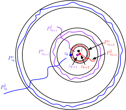
Figure 2: Illustration of the proof of (2) of Lemma 3.6. The union of the paths $P_{k}^{\circ}(z_{k})$ and $P_{k}^{\parallel}(z_{k})$ from conditions A and B for three consecutive values of $k$ is connected. To get (2), we sum the $D_{h}$-lengths of these paths over all $k\in\{m-1,\dots,n-2\}$.

Proof of Lemma 3.6.

Step 1: proof of (3.20). For $z\in U$ and $n\in\mathbbm{N}$, let $z_{n}\in(e^{-n-100}\mathbbm{Z}^{2})\cap U$ be as in Lemma 3.7. By (3.24) and (3.26), if $t\in[n+1,n+2]$ such that $h_{e^{-t}}(z)\geq 2t-\alpha\log t$, then

$$h_{e^{-t}}(z)\leq 2n-\alpha_{0}\log n+2\mathopen{}\mathclose{{}\left|\alpha\log t}\right|^{1/2+\zeta}+\log C_{0}+C_{1}.$$ (3.31)

Since $\alpha<\alpha_{0}$, this last quantity is smaller than $2t-\alpha\log t$ if $n$ is sufficiently large (how large is random and does not depend on $z$). Hence, there exists a random $n_{*}\in\mathbbm{N}$ such that for each $n\geq n_{*}$, we have $h_{e^{-t}}(z)\leq 2t-\alpha\log t$ for each $t\in[n+1,n+2]$ and each $z\in U$. By the continuity of the circle average process, the quantity $\sup_{z\in U}\sup_{t\in[0,n_{*}+1]}|h_{e^{-t}}(z)|$ is a.s. finite. By choosing $C$ to be 100 times this quantity, say, we get (3.20).

Step 2: bounding lengths of paths. By applying (3.26) and (3.27) to estimate the right side of (3.23), we get that for each $t\in[n+1,n+2]$, the $D_{h}$-lengths of the paths $P^{\circ}_{n}(z_{n})$ and $P^{\parallel}_{n}(z_{n})$ from conditions A and B are each bounded above by

$$C_{0}\exp\mathopen{}\mathclose{{}\left(\xi h_{e^{-n}}(z)-\xi Qn+\mathopen{}\mathclose{{}\left|2n-h_{e^{-n}}(z)}\right|^{1/2+\zeta}}\right)$$

$$\qquad\leq C_{0}\exp\mathopen{}\mathclose{{}\left(\xi h_{e^{-t}}(z)-\xi Qn+(2+2\xi)\mathopen{}\mathclose{{}\left|2t-h_{e^{-t}}(z)}\right|^{1/2+\zeta}+2C_{1}}\right)$$

$$\qquad\leq C_{0}e^{2C_{1}+2\xi Q}\exp\mathopen{}\mathclose{{}\left(\xi h_{e^{-t}}(z)-\xi Qt+(2+2\xi)\mathopen{}\mathclose{{}\left|2t-h_{e^{-t}}(z)}\right|^{1/2+\zeta}}\right).$$

Hence, the $D_{h}$-lengths of each of these paths is bounded above by

$$C\min_{t\in[n+1,n+2]}\exp\mathopen{}\mathclose{{}\left(\xi h_{e^{-t}}(z)-\xi Qt+(2+2\xi)\mathopen{}\mathclose{{}\left|2t-h_{e^{-t}}(z)}\right|^{1/2+\zeta}}\right)$$ (3.32)

for $C=C_{0}e^{2C_{1}+2\xi Q}$.

Step 3: proof of (3). For $n\in\mathbbm{N}$, then path $P^{\circ}_{n}(z_{n})$ disconnects the inner and outer boundaries of the annulus $A_{z_{n}}^{\circ}(e^{-n})=A_{z_{n}}(e^{-n-51/100},e^{-n-1/2})$. Since $|z-z_{n}|\leq e^{-n-99}$, this path also disconnects the inner and outer boundaries of the annulus $\mathbbm{A}_{z}(e^{-n-1},e^{-n})$. Hence (3) follows from (3.32) for $P_{n}^{\circ}(z_{n})$.

Step 4: proof of (2). Let $n,m\in\mathbbm{N}$ with $m<n$. We will prove (2) by chaining together the paths $P_{k}^{\circ}(z_{k})$ and $P_{k}^{\parallel}(z_{k})$ from conditions B and A above for $k\in\{m-1,\dots,n-2\}$, where $z_{k}$ is as in Lemma 3.7. See Figure 2 for an illustration.

For each $k\in\{m-1,\dots,n-2\}$, the path $P_{k}^{\parallel}(z_{k})$ goes from $\partial B_{z_{k}}(e^{-k-100})$ to $\partial B_{z_{k}}(e^{-k})$. We have

$$|z_{k+1}-z_{k}|\leq|z_{k+1}-z|+|z_{k}-z|\leq 2e^{-k-99},$$

so the annuli $A_{z_{k}}^{\circ}(e^{-k})$ and $A_{z_{k+1}}^{\circ}(e^{-k-1})$ are each contained in $\mathbbm{A}_{z_{k}}(e^{-k},e^{-k-100})$ and disconnect the inner and outer boundaries of this last annulus. Hence $P_{k}^{\parallel}(z_{k})$ intersects the paths $P_{k}^{\circ}(z_{k})$ and $P_{k+1}^{\circ}(z_{k+1})$. Therefore, the union of the paths $P_{k}^{\parallel}(z_{k})$ and $P_{k}^{\circ}(z_{k})$ for $k\in\{m-1,\dots,n-2\}$ is connected. Furthermore, since $|z-z_{m-1}|\leq e^{-m-98}$ and $|z-z_{n-2}|\leq e^{-n-97}$, the path $P_{m-1}^{\parallel}(z_{m-1})$ intersects $\partial B_{z}(e^{-m})$ and the path $P_{n-2}^{\parallel}(z_{n-2})$ intersects $\partial B_{z}(e^{-n-50})$. Hence summing the estimate (3.32) gives

$$D_{h}\mathopen{}\mathclose{{}\left(\partial B_{z}(e^{-n-50}),\partial B_{z}(e^{-m})}\right)$$

$$\qquad\qquad\leq 2C\sum_{k=m-1}^{n-2}\min_{t\in[k+1,k+2]}\exp\mathopen{}\mathclose{{}\left(\xi h_{e^{-t}}(z)-\xi Qt+(2+2\xi)\mathopen{}\mathclose{{}\left|2t-h_{e^{-t}}(z)}\right|^{1/2+\zeta}}\right)$$

$$\qquad\qquad=2C\sum_{k=m}^{n-1}\min_{t\in[k,k+1]}\exp\mathopen{}\mathclose{{}\left(\xi h_{e^{-t}}(z)-\xi Qt+(2+2\xi)\mathopen{}\mathclose{{}\left|2t-h_{e^{-t}}(z)}\right|^{1/2+\zeta}}\right).$$

∎

3.3 Specializing to the case when $Q=2$

We henceforth assume that $\xi=\xi_{\mathrm{c}}$, equivalently $Q=2$. In this special case, the estimates of Lemma 3.6 can be simplified.

Lemma 3.8.

Let $U\subset\mathbbm{C}$ be a bounded open set and let $\delta\in(0,\xi_{\mathrm{c}})$. Almost surely, there exists a random $C\in(0,\infty)$ such that the following is true for each $z\in U$.

1. For each $n,m\in\mathbbm{N}$ with $m<n$,

   $$D_{h}\mathopen{}\mathclose{{}\left(\partial B_{z}(e^{-n-50}),\partial B_{z}(e^{-m})}\right)\leq C\sum_{k=m}^{n-1}\min_{t\in[k,k+1]}\exp\mathopen{}\mathclose{{}\left((\xi_{\mathrm{c}}-\delta)(h_{e^{-t}}(z)-2t)}\right).$$ (3.33)

2. For each $n\in\mathbbm{N}$,

   $$D_{h}\mathopen{}\mathclose{{}\left(\text{around $\mathbbm{A}_{z}(e^{-n-1},e^{-n})$}}\right)\leq C\min_{t\in[n+1,n+2]}\exp\mathopen{}\mathclose{{}\left((\xi_{\mathrm{c}}-\delta)(h_{e^{-t}}(z)-2t)}\right).$$ (3.34)

Proof.

Let $\alpha\in(0,1/4)$ and $\zeta\in(0,1/2)$. By (3.20) of Lemma 3.6, a.s. there is a random $C\in(0,\infty)$ such that for each $z\in U$,

$$2t-h_{e^{-t}}(z)\geq\alpha\log t-C,\quad\forall t\geq 0.$$ (3.35)

By (3.35), for each large enough $t>0$ it holds for each $z\in U$ that

$$2t-h_{e^{-t}}(z)\geq 0\quad\text{and}\quad(2t-h_{e^{-t}}(z))^{1/2-\zeta}\geq(2+2\xi_{\mathrm{c}})/\delta.$$

Equivalently, the error term inside the exponential in (2) and (3) in Lemma 3.6 satisfies

$$(2+2\xi_{\mathrm{c}})\mathopen{}\mathclose{{}\left|2t-h_{e^{-t}}(z)}\right|^{1/2+\zeta}\leq\delta(2t-h_{e^{-t}}(z)).$$ (3.36)

By plugging (3.36) into (2) and (3) from Lemma 3.6, recalling that $Q=2$, and possibly increasing $C$ to deal with the bounded interval of $t$-values for which (3.36) does not hold, we get (3.33) and (3.34). ∎

We have the following simplified form of (3.34) from Lemma 3.8.

Lemma 3.9.

Let $U\subset\mathbbm{C}$ be a bounded open set and let $\theta\in(0,\xi_{\mathrm{c}}/4)$. Almost surely, there is a random $C\in(0,\infty)$ such that for each $z\in U$ and each $n\in\mathbbm{N}$,

$$D_{h}\mathopen{}\mathclose{{}\left(\text{around $\mathbbm{A}_{z}(e^{-n-1},e^{-n})$}}\right)\leq Cn^{-\theta}.$$ (3.37)

Proof.

Let $\delta\in(0,\xi_{\mathrm{c}})$ and $\alpha\in(0,1/4)$ to be chosen later, depending on $\theta$. The estimate (3.34) from Lemma 3.8 combined with (3.20) from Lemma 3.6 shows that a.s. there is a random $C\in(0,\infty)$ such that for each $z\in U$ and each $n\in\mathbbm{N}$,

$$D_{h}\mathopen{}\mathclose{{}\left(\text{around $\mathbbm{A}_{z}(e^{-n-1},e^{-n})$}}\right)\leq C\exp\mathopen{}\mathclose{{}\left(-(\xi_{\mathrm{c}}-\delta)\alpha\log n}\right)=Cn^{-(\xi_{\mathrm{c}}-\delta)\alpha}.$$ (3.38)

We conclude the proof by choosing $\delta$ sufficiently close to 0 and $\alpha$ sufficiently close to $1/4$ so that $(\xi_{\mathrm{c}}-\delta)\alpha\geq\theta$. ∎

3.4 Distances between scales for “good” and “bad” points

We now seek to estimate the sum appearing on the right side of (3.33). We first consider the easy case, when $h_{e^{-t}}(z)$ does not get too close to $2t$.

Lemma 3.10.

Let $U\subset\mathbbm{C}$ be a bounded open set, let $\theta>0$, and let $\beta>(1+\theta)/\xi_{\mathrm{c}}$. Almost surely, there is a random $C\in(0,\infty)$ such that for each $z\in U$ and each $n,m\in\mathbbm{N}$ with $m<n$ such that

$$h_{e^{-t}}(z)-h_{1}(z)\leq 2t-\beta\log t,\quad\forall t\in[m,n]_{\mathbbm{Z}},$$ (3.39)

it holds that

$$D_{h}\mathopen{}\mathclose{{}\left(\partial B_{z}(e^{-n-50}),\partial B_{z}(e^{-m})}\right)\leq Cm^{-\theta}.$$ (3.40)

Note that, unlike in most of the other lemma statements in this subsection, we allow a general choice of $\theta>0$ in Lemma 3.10 rather than requiring $\theta\in(0,\xi_{\mathrm{c}}/4)$.

Proof of Lemma 3.10.

Let $\delta\in(0,\xi_{\mathrm{c}})$ be small. By Lemma 3.8, a.s. there exists a random $C_{0}\in(0,\infty)$ such that for each $z\in U$ satisfying (3.39),

$$D_{h}\mathopen{}\mathclose{{}\left(B_{z}(e^{-n-50}),\partial B_{z}(e^{-m})}\right) \leq C_{0}\sum_{k=m}^{n-1}\min_{t\in[k,k+1]}\exp\mathopen{}\mathclose{{}\left((\xi_{\mathrm{c}}-\delta)(h_{e^{-t}}(z)-2t)}\right)$$

$$\leq C_{0}\sum_{k=m}^{n-1}\min_{t\in[k,k+1]}\exp\mathopen{}\mathclose{{}\left((\xi_{\mathrm{c}}-\delta)(h_{1}(z)-\beta\log t)}\right)\quad\text{(by~{}\eqref{eqn-good-pt-dist-interval})}$$

$$\leq C_{0}\exp\mathopen{}\mathclose{{}\left((\xi_{\mathrm{c}}-\delta)\sup_{w\in U}|h_{1}(w)|}\right)\sum_{k=m}^{n-1}k^{-(\xi_{\mathrm{c}}-\delta)\beta}\quad$$

$$\leq Cm^{-(\xi_{\mathrm{c}}-\delta)\beta+1}$$ (3.41)

for some random $C>0$, where in the last line we use that $\sup_{w\in U}|h_{1}(w)|$ is a.s. finite and $(\xi_{\mathrm{c}}-\delta)\beta>1$. Since $\beta>(1+\theta)/\xi_{\mathrm{c}}$, the exponent on the right side of (3.4) is less than $-\theta$ provided $\delta$ is chosen to be small enough. ∎

Lemma 3.10 is not sufficient for our purposes since a.s. there are points $z\in U$ and arbitrarily small radii $e^{-t}$ for which $h_{e^{-t}}(z)-h_{1}(z)\geq 2t-\mathopen{}\mathclose{{}\left(\frac{3}{4}+o_{t}(1)}\right)\log t$ (see Proposition 2.5). We have $3/4<1/\xi_{\mathrm{c}}$, so we cannot take $\beta\leq 3/4$ in Lemma 3.10. Hence we need an alternative estimate to deal with points $z\in U$ for which $h_{e^{-t}}(z)-h_{1}(z)$ gets very close to $2t$ for some $t\in[m,n]$. We first consider the case when this happens at the right endpoint, i.e., $h_{e^{-n}}(z)-h_{1}(z)\geq 2n-\beta\log n$ for an appropriate $\beta>0$. We will eventually reduce to the case when $h_{e^{-n}}(z)-h_{1}(z)$ is large by considering the largest value of $t\in[m,n]$ for which $h_{e^{-t}}(z)-h_{1}(z)\geq 2t-\beta\log t$. In fact, for our purposes it is enough to take $m=\lfloor n/2\rfloor$.

Lemma 3.11.

Let $U\subset\mathbbm{C}$ be a bounded open set, let $\theta\in(0,\xi_{\mathrm{c}}/4)$, and let $\beta>(1+\theta)/\xi_{\mathrm{c}}$. Almost surely, there is a random constant $C\in(0,\infty)$ such that for each $n\in\mathbbm{N}$ and each $z\in(e^{-n-100}\mathbbm{Z}^{2})\cap U$ such that

$$h_{e^{-n}}(z)-h_{1}(z)\geq 2n-\beta\log n,$$ (3.42)

we have

$$D_{h}\mathopen{}\mathclose{{}\left(\partial B_{z}(e^{-n}),\partial B_{z}(e^{-n/2})}\right)\leq Cn^{-\theta}.$$ (3.43)

Intuitively, the reason why the condition (3.42) helps us get a better estimate is that (by the Gaussian tail bound) the probability that $h_{e^{-n}}(z)-h_{1}(z)\geq 2n-\beta\log n$ is small. So, there will not be very many points $z\in(e^{-n-100}\mathbbm{Z}^{2})\cap U$ for which (3.42) holds, and we can take a union bound over all of them. The key inputs in the proof of Lemma 3.11 are Lemma 3.8 and the following estimate for a Brownian bridge, which we will apply to the conditional law of $\{h_{e^{-t}}(z)-h_{1}(z)\}_{t\in[0,n]}$ given $h_{e^{-n}}(z)-h_{1}(z)$.

Lemma 3.12.

Fix $\beta>\alpha>0$. Let $T>0$, let $x\in[\alpha\log T,\beta\log T]$, and let $W$ be a Brownian bridge from 0 to $2T-x$ in time $T$. For $S>0$,

$$\mathbbm{P}\mathopen{}\mathclose{{}\left[W_{t}\leq 2t-\alpha\log T\>\forall t\in[T/2,T],\>\int_{T/2}^{T}\mathbbm{1}_{(W_{t}\geq 2t-\beta\log T)}\,dt>S}\right]\leq c_{0}\exp\mathopen{}\mathclose{{}\left(-c_{1}\frac{S}{(\log T)^{2}}}\right)$$ (3.44)

for constants $c_{0},c_{1}>0$ depending only on $\alpha,\beta$.

In the application we have in mind, we will take $\alpha\in(0,1/4)$, $\beta>(1+\theta)/\xi_{\mathrm{c}}$ as in Lemma 3.10, and $T=n$. Our Brownian bridge $W_{t}=h_{e^{-t}}(z)-h_{1}(z)$ (conditioned on $h_{e^{-n}}(z)-h_{1}(z)$) will be forced to stay below $2t-\alpha\log n$ for $t\in[n/2,n]$ by Proposition 2.4 (in the form of (3.20) of Lemma 3.6). Hence Lemma 3.12 will provide an upper bound on the Lebesgue measure of the set of times $t\in[n/2,n]$ for which $h_{e^{-t}}(z)-h_{1}(z)\geq 2t-\beta\log n$. This will allow us to upper-bound the sum on the right side of (3.33).

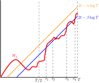
Figure 3: Illustration of the proof of Lemma 3.12. The time $\tau_{1}$ is the first time after $T/2$ for which $W_{t}\geq 2t-\beta\log T$ and the time $\tau_{k}$ is the first time after $\tau_{k-1}+(\log T)^{2}$ for which $W_{t}\geq 2t-\beta\log T$, or $\tau_{k}=T$ if no such time exists. Note that we may have $W_{\tau_{k}}>2\tau_{k}-\beta\log T$, as is the case for $\tau_{2}$ in the figure. The idea of the proof is that in each interval $[\tau_{k},\tau_{k}+(\log T)^{2}]$ there is a chance that $W_{t}$ goes above $2t-\alpha\log T$. From this and an independence argument, we get it is very unlikely that many of the times $\tau_{k}$ are strictly less than $T$ and $W_{t}\leq 2t-\alpha\log T$ for all $t\in[T/2,T]$.

Proof of Lemma 3.12.

The idea of the proof is that if $t$ is such that $W_{t}\geq 2t-\beta\log T$, then by a basic Gaussian estimate there is a positive chance that $W_{t+(\log T)^{2}}$ will be larger than $2t-\alpha\log T$. So, it is very unlikely that $W$ spends a lot of time above $2t-\beta\log T$ while simultaneously staying below $2t-\alpha\log T$. See Figure 3 for an illustration.

Step 1: setup. To simplify the calculations, we will first reduce to a Brownian bridge from 0 to 0. We can write

$$W_{t}=\mathring{W}_{t}+\frac{t}{T}(2T-x)=\mathring{W}_{t}+2t-\frac{t}{T}x$$

where $\mathring{W}$ is a Brownian bridge from 0 to 0 in time $T$. The event whose probability we seek to bound can be written in terms of $\mathring{W}$ as

$$G=\mathopen{}\mathclose{{}\left\{\mathring{W}_{t}\leq\frac{t}{T}x-\alpha\log T\>\forall t\in[T/2,T],\>\int_{T/2}^{T}\mathbbm{1}\mathopen{}\mathclose{{}\left\{\mathring{W}_{t}\geq\frac{t}{T}x-\beta\log T}\right\}\,dt>S}\right\}.$$ (3.45)

Let

$$\tau_{1}:=T\wedge\inf\mathopen{}\mathclose{{}\left\{t\geq T/2:\mathring{W}_{t}\geq\frac{t}{T}x-\beta\log T}\right\}.$$

For $k\geq 2$, inductively let

$$\tau_{k}:=T\wedge\inf\mathopen{}\mathclose{{}\left\{t\geq\tau_{k-1}+(\log T)^{2}:\mathring{W}_{t}\geq\frac{t}{T}x-\beta\log T}\right\}.$$ (3.46)

Step 2: reducing to a bound for an event involving the $\tau_{k}$s. We will now upper-bound the probability of the event $G$ of (3.45) in terms of the $\tau_{k}$s. To this end, let

$$E_{k}:=\mathopen{}\mathclose{{}\left\{\tau_{k}\leq T-2(\log T)^{2},\>\mathring{W}_{\tau_{k}+(\log T)^{2}}>\frac{\tau_{k}+(\log T)^{2}}{T}x-\alpha\log T}\right\}.$$ (3.47)

Note that $E_{k}\in\sigma(\mathring{W}|_{[0,\tau_{k+1}]})$. Furthermore, if $E_{k}$ occurs for any $k\in\mathbbm{N}$, then the first condition in the event $G$ of (3.45) does not occur. Hence

$$G\subset\bigcap_{k=1}^{\infty}E_{k}^{c}.$$ (3.48)

Let

$$K:=\max\mathopen{}\mathclose{{}\left\{k\in\mathbbm{N}:\tau_{k}\leq T-2(\log T)^{2}}\right\}.$$ (3.49)

If $t\in[T/2,T]$ does not belong $\bigcup_{k=1}^{K}[\tau_{k},\tau_{k}+(\log T)^{2}]\cup[T-2(\log T)^{2},T]$, then $\mathring{W}_{t}\leq\frac{t}{T}x-\beta\log T$. Consequently,

$$\int_{T/2}^{T}\mathbbm{1}\mathopen{}\mathclose{{}\left\{\mathring{W}_{t}\geq\frac{t}{T}x-\beta\log T}\right\}\,dt\leq(K+2)(\log T)^{2}.$$

By (3.48) and the definition (3.45) of $G$, we therefore have

$$G\subset\bigcap_{k=1}^{\infty}E_{k}^{c}\cap\mathopen{}\mathclose{{}\left\{K>\frac{S}{(\log T)^{2}}-2}\right\}.$$ (3.50)

Step 3: proof conditional on a Brownian bridge calculation. Let us now bound the probability of the event on the right side of (3.50). Just below, we will show via an elementary Brownian bridge calculation that there is a constant $p=p(\alpha,\beta)\in(0,1)$ such that for each $k\in\{0,1,2,\dots\}$, it holds a.s. on the event $\{\tau_{k}\leq T-2(\log T)^{2}\}$ that

$$\mathbbm{P}\mathopen{}\mathclose{{}\left[E_{k}\,|\,\mathring{W}|_{[0,\tau_{k}]}}\right]\geq p.$$ (3.51)

Since $\{\tau_{k}\leq T-2(\log T)^{2}\}\subset E_{k}$ and $E_{j}\in\sigma\mathopen{}\mathclose{{}\left(\mathring{W}|_{[0,\tau_{k}]}}\right)$ for each $j\in\{1,\dots,k-1\}$, we deduce from (3.51) that

$$\mathbbm{P}\mathopen{}\mathclose{{}\left[E_{k}^{c}\cap\{\tau_{k}\leq T-2(\log T)^{2}\}\,|\,\bigcap_{j=1}^{k-1}E_{j}^{c}\cap\{\tau_{k-1}\leq T-2(\log T)^{2}\}}\right]$$

$$\qquad\qquad\leq\mathbbm{P}\mathopen{}\mathclose{{}\left[E_{k}^{c}\,|\,\bigcap_{j=1}^{k-1}E_{j}^{c}\cap\{\tau_{k}\leq T-2(\log T)^{2}\}}\right]$$

$$\qquad\qquad\leq 1-p.$$ (3.52)

Iterating the estimate (3.4) $k$ times gives

$$\mathbbm{P}\mathopen{}\mathclose{{}\left[\tau_{k}\leq T-2(\log T)^{2},\>\bigcap_{j=1}^{k}E_{j}^{c}}\right]\leq(1-p)^{k}.$$ (3.53)

We now take $k=\lceil\frac{S}{(\log T)^{2}}-2\rceil$ in (3.53) and recall the definition (3.49) of $K$ to get

$$\mathbbm{P}\mathopen{}\mathclose{{}\left[\bigcap_{k=1}^{\infty}E_{k}^{c}\cap\mathopen{}\mathclose{{}\left\{K>\frac{S}{(\log T)^{2}}-2}\right\}}\right]\leq c_{0}\exp\mathopen{}\mathclose{{}\left(-c_{1}\frac{S}{(\log T)^{2}}}\right)$$

for constants $c_{0},c_{1}>0$ depending only on $\alpha,\beta$. Combining this with (3.50) concludes the proof.

Step 4: Brownian bridge calculation. It remains to prove (3.51). The proof is an elementary application of the formulas for the mean and variance of a Brownian bridge with given endpoints, together with some straightforward estimates.

If we condition on $\mathring{W}|_{[0,\tau_{k}]}$, then the conditional law of $\mathring{W}_{\cdot+\tau_{k}}$ is that of a Brownian bridge from $\mathring{W}_{\tau_{k}}$ to 0 in time $T-\tau_{k}$. In particular, if $\tau_{k}<T-(\log T)^{2}$, then the conditional law of $\mathring{W}_{\tau_{k}+(\log T)^{2}}$ is Gaussian with mean

$$\mathopen{}\mathclose{{}\left(1-\frac{(\log T)^{2}}{T-\tau_{k}}}\right)\mathring{W}_{\tau_{k}}$$ (3.54)

and variance

$$(\log T)^{2}-\frac{(\log T)^{4}}{T-\tau_{k}}.$$ (3.55)

We will now estimate the above formulas for the conditional mean and variance. Recall that $T/2\leq\tau_{k}\leq T$ and $\mathring{W}_{\tau_{k}}\geq\frac{\tau_{k}}{T}x-\beta\log T$ by (3.46) and $x\in[\alpha\log T,\beta\log T]$ by definition. In particular,

$$\frac{\tau_{k}}{T}x-\beta\log T\leq x-\beta\log T\leq 0.$$

Hence

$$\mathbbm{E}\mathopen{}\mathclose{{}\left[\mathring{W}_{\tau_{k}+(\log T)^{2}}\,|\,\mathring{W}|_{[0,\tau_{k}]}}\right] =\mathopen{}\mathclose{{}\left(1-\frac{(\log T)^{2}}{T-\tau_{k}}}\right)\mathring{W}_{\tau_{k}}$$

$$\geq\mathopen{}\mathclose{{}\left(1-\frac{(\log T)^{2}}{T-\tau_{k}}}\right)\mathopen{}\mathclose{{}\left(\frac{\tau_{k}}{T}x-\beta\log T}\right)$$

$$\geq\frac{\tau_{k}}{T}x-\beta\log T\quad\text{(since $\frac{\tau_{k}}{T}x-\beta\log T\leq 0$)}$$

$$\geq\frac{1}{2}x-\beta\log T\quad\text{(since $\tau_{k}\geq T/2$)}$$

$$\geq(\alpha/2-\beta)\log T\quad\text{(since $x\geq\alpha\log T$)}.$$ (3.56)

Furthermore, using (3.55), we see that if $\tau_{k}\leq T-2(\log T)^{2}$, then

$$\operatorname{Var}\mathopen{}\mathclose{{}\left[\mathring{W}_{\tau_{k}+(\log T)^{2}}\,|\,\mathring{W}|_{[0,\tau_{k}]}}\right]\geq\frac{1}{2}(\log T)^{2}.$$ (3.57)

On the event $\{\tau_{k}\leq T-2(\log T)^{2}\}$, the quantity appearing in the definition (3.47) of $E_{k}$ satisfies

$$\frac{\tau_{k}+(\log T)^{2}}{T}x-\alpha\log T\leq x-\alpha\log T\leq(\beta-\alpha)\log T.$$ (3.58)

Hence, on this event

$$\mathbbm{P}\mathopen{}\mathclose{{}\left[E_{k}\,|\,\mathring{W}|_{[0,\tau_{k}]}}\right] \geq\mathbbm{P}\mathopen{}\mathclose{{}\left[\mathring{W}_{\tau_{k}+(\log T)^{2}}>(\beta-\alpha)\log T\,|\,\mathring{W}|_{[0,\tau_{k}]}}\right]\quad\text{(by~{}\eqref{eqn-bridge-threshold})}$$

$$\geq p\quad\text{(by~{}\eqref{eqn-bridge-cond-mean} and~{}\eqref{eqn-bridge-cond-var})},$$

where $p\in(0,1)$ depends only on $\alpha,\beta$. ∎

Proof of Lemma 3.11.

Let us first explain the main idea of the proof. For a small $\delta\in(0,\xi_{\mathrm{c}})$, Lemma 3.8 gives the bound

$$D_{h}\mathopen{}\mathclose{{}\left(\partial B_{z}(e^{-n}),\partial B_{z}(e^{-n/2})}\right)\leq C\int_{\lfloor n/2\rfloor}^{n}\exp\mathopen{}\mathclose{{}\left((\xi_{\mathrm{c}}-\delta)(h_{e^{-t}}(z)-2t)}\right)\,dt$$ (3.59)

for a random $C\in(0,\infty)$ (which does not depend on $z$ and $n$). To estimate the integral on the right side of (3.59), we consider separately the integrals over the “good” set of $t\in[\lfloor n/2\rfloor,n]$ where $h_{e^{-t}}(z)-2t\leq-\beta\log n$ and the “bad” set where $h_{e^{-t}}(z)-2t>-\beta\log n$. The integral over the “good” set is bounded above by a constant times $n^{-\theta}$ by our choice of $\beta$. Proposition 2.4 together with Lemma 3.12 will allow us to show that the Lebesgue measure of the “bad” set is small. Furthermore, Proposition 2.4 (in the form of Lemma 3.6) shows that if $\alpha\in(0,1/4)$, then when $n$ is sufficiently large, we have $h_{e^{-t}}(z)-2t\leq-\alpha\log n$ for each $t\in[\lfloor n/2\rfloor,n]$. These two facts will allow us to upper-bound the integral over the “bad” set by a constant times $n^{-\theta}$ as well. Let us now proceed with the details.

Step 1: setup. Let $\alpha\in(0,1/4)$ (we will eventually take $\alpha$ to be very close to $1/4$, depending on $\theta$). By (3.20) of Lemma 3.6 applied with $\alpha^{\prime}\in(\alpha,1/4)$ in place of $\alpha$, a.s. there exists a random $t_{*}\in\mathbbm{N}$ such that for each $z\in U$,

$$h_{e^{-t}}(z)-h_{1}(z)\leq 2t-\alpha\log(2t),\quad\forall t\geq t_{*}.$$ (3.60)

For $n\in\mathbbm{N}$ and $z\in U$, let

$$G_{n}(z) :=\mathopen{}\mathclose{{}\left\{h_{e^{-t}}(z)-h_{1}(z)\leq 2t-\alpha\log n\>\forall t\in[n/2,n]}\right\}$$

$$\qquad\cap\mathopen{}\mathclose{{}\left\{\int_{n/2}^{n}\mathbbm{1}\mathopen{}\mathclose{{}\left\{h_{e^{-t}}(z)-h_{1}(z)\geq 2t-\beta\log n}\right\}\,dt>(\log n)^{4}}\right\}.$$ (3.61)

Note that by (3.60), a.s. for each large enough $n\in\mathbbm{N}$ the first event in the definition (3.4) occurs for every $z\in U$. The event $G_{n}(z)$ should be compared to the event of Lemma 3.12.

Step 2: bound for the probability of $G_{n}(z)\cap\{h_{e^{-n}}(z)-h_{1}(z)\in[2n-\beta\log n,2n-\alpha\log n]\}$. By the calculations in [DS11, Section 3.1], for each fixed $z\in U$, the process $t\mapsto h_{e^{-t}}(z)-h_{1}(z)$ is a standard linear Brownian motion. In particular, if $n\in\mathbbm{N}$, $z\in U$, and $x\in[\alpha\log n,\beta\log n]$, then the conditional distribution of $t\mapsto h_{e^{-t}}(z)-h_{1}(z)$ given $\{h_{e^{-n}}(z)-h_{1}(z)=2n-x\}$ is that of a Brownian bridge from 0 to $2n-x$ in time $n$. By Lemma 3.12 applied with $T=n$ and $S=(\log n)^{4}$, we therefore obtain

$$\mathbbm{P}\mathopen{}\mathclose{{}\left[G_{n}(z)\,|\,h_{e^{-n}}(z)-h_{1}(z)\in[2n-\beta\log n,2n-\alpha\log n]}\right]\leq c_{0}\exp\mathopen{}\mathclose{{}\left(-c_{1}(\log n)^{2}}\right)$$ (3.62)

for constants $c_{0},c_{1}>0$ depending only on $\alpha,\beta$. Since $h_{e^{-n}}(z)-h_{1}(z)$ is centered Gaussian with variance $n$, we also have

$$\mathbbm{P}\mathopen{}\mathclose{{}\left[h_{e^{-n}}(z)-h_{1}(z)\geq 2n-\beta\log n}\right]\leq\exp\mathopen{}\mathclose{{}\left(-\frac{(2n-\beta\log n)^{2}}{2n}}\right)\leq\exp\mathopen{}\mathclose{{}\left(-2n}\right)n^{2\beta}.$$ (3.63)

By (3.62) and (3.63), for each $z\in U$,

$$\mathbbm{P}\mathopen{}\mathclose{{}\left[G_{n}(z),\,h_{e^{-n}}(z)-h_{1}(z)\in[2n-\beta\log n,2n-\alpha\log n]}\right]\leq c_{0}\exp\mathopen{}\mathclose{{}\left(-2n-c_{1}(\log n)^{2}}\right)n^{2\beta}.$$ (3.64)

Step 3: a.s. bounds for points $z$ such that $h_{e^{-n}}(z)-h_{1}(z)\geq 2n-\beta\log n$. By (3.64) and a union bound over $O_{n}(e^{-2n})$ choices of $z\in(e^{-n-100}\mathbbm{Z}^{2})\cap U$, it holds with probability at least $1-O_{n}\mathopen{}\mathclose{{}\left(e^{-c_{1}(\log n)^{2}}n^{2\beta}}\right)$ that for each such $z$, either $G_{n}(z)$ does not occur or $h_{e^{-n}}(z)-h_{1}(z)\notin[2n-\beta\log n,2n-\alpha\log n]$. Recalling the definition (3.4) of $G_{n}(z)$, we see that this implies that with probability at least $1-O_{n}\mathopen{}\mathclose{{}\left(e^{-c_{1}(\log n)^{2}}n^{2\beta}}\right)$, at least one of the following three conditions holds for each $z\in(e^{-n-100}\mathbbm{Z}^{2})\cap U$:

1. $h_{e^{-n}}(z)-h_{1}(z)<2n-\beta\log n$;

2. If we let

   $$H_{n}(z,t):=\mathopen{}\mathclose{{}\left\{h_{e^{-t}}(z)-h_{1}(z)\geq 2t-\beta\log n}\right\},$$ (3.65)

   then $\int_{n/2}^{n}\mathbbm{1}_{H_{n}(z,t)}\,dt\leq(\log n)^{4}$; or

3. $h_{e^{-t}}(z)-h_{1}(z)>2t-\alpha\log n$ for some $t\in[n/2,n]$.

By the Borel-Cantelli lemma, a.s. this trichotomy holds for all large enough $n\in\mathbbm{N}$.

By (3.60), a.s. for each large enough $n\in\mathbbm{N}$ the condition (iii) is not satisfied for any $z\in(e^{-n-100}\mathbbm{Z}^{2})\cap U$. Therefore, it is a.s. the case that for each large enough $n\in\mathbbm{N}$, it holds for each $z\in(e^{-n-100}\mathbbm{Z}^{2})\cap U$ such that $h_{e^{-n}}(z)-h_{1}(z)\geq 2n-\beta\log n$ that

$$h_{e^{-t}}(z)-h_{1}(z)\leq 2t-\alpha\log n,\>\forall t\in[n/2,n]\quad\text{and}\quad\int_{n/2}^{n}\mathbbm{1}_{H_{n}(z,t)}\,dt\leq(\log n)^{4}.$$ (3.66)

Step 4: splitting up the integral. Now let $\delta\in(0,\xi_{\mathrm{c}})$ be small. By Lemma 3.8, a.s. there exists $C\in(0,\infty)$ such that for each $n\in\mathbbm{N}$ and each $z\in U$,

$$D_{h}\mathopen{}\mathclose{{}\left(\partial B_{z}(e^{-n-50}),\partial B_{z}(e^{-n/2})}\right) \leq C\sum_{k=\lfloor n/2\rfloor}^{n-1}\min_{t\in[k,k+1]}\exp\mathopen{}\mathclose{{}\left((\xi_{\mathrm{c}}-\delta)(h_{e^{-t}}(z)-2t)}\right)$$

$$\leq C\int_{\lfloor n/2\rfloor}^{n}\exp\mathopen{}\mathclose{{}\left((\xi_{\mathrm{c}}-\delta)(h_{e^{-t}}(z)-2t)}\right)\,dt.$$ (3.67)

We now break up the integral on the right side of (3.4) based on whether or not the event $H_{n}(z,t)$ from (3.65) occurs. Using (3.66) and (3.4), we get that a.s. for each large enough $n\in\mathbbm{N}$ and each $z\in(e^{-n-100}\mathbbm{Z}^{2})\cap U$ such that $h_{e^{-n}}(z)-h_{1}(z)\geq 2n-\beta\log n$,

$$D_{h}\mathopen{}\mathclose{{}\left(B_{z}(e^{-n-50}),\partial B_{z}(e^{-n/2})}\right)$$

$$\qquad\leq C\int_{\lfloor n/2\rfloor}^{n}\exp\mathopen{}\mathclose{{}\left((\xi_{\mathrm{c}}-\delta)(h_{e^{-t}}(z)-2t)}\right)\mathbbm{1}_{H_{n}(z,t)}\,dt$$

$$\qquad\qquad+C\int_{\lfloor n/2\rfloor}^{n}\exp\mathopen{}\mathclose{{}\left((\xi_{\mathrm{c}}-\delta)(h_{e^{-t}}(z)-2t)}\right)\mathbbm{1}_{H_{n}(z,t)^{c}}\,dt$$

$$\qquad\leq C\int_{\lfloor n/2\rfloor}^{n}\exp\mathopen{}\mathclose{{}\left((\xi_{\mathrm{c}}-\delta)(h_{1}(z)-\alpha\log n)}\right)\mathbbm{1}_{H_{n}(z,t)}\,dt$$

$$\qquad\qquad+C\int_{\lfloor n/2\rfloor}^{n}\exp\mathopen{}\mathclose{{}\left((\xi_{\mathrm{c}}-\delta)(h_{1}(z)-\beta\log n)}\right)\mathbbm{1}_{H_{n}(z,t)^{c}}\,dt\quad\text{(by~{}\eqref{eqn-trichotomy-int} and~{}\eqref{eqn-bad-pt-dichotomy})}$$

$$\qquad\leq C\exp\mathopen{}\mathclose{{}\left((\xi_{\mathrm{c}}-\delta)\sup_{z\in U}h_{1}(z)}\right)\mathopen{}\mathclose{{}\left[n^{-\alpha(\xi_{\mathrm{c}}-\delta)}\int_{\lfloor n/2\rfloor}^{n+2}\mathbbm{1}_{H_{n}(z,t)}\,dt+n^{-\beta(\xi_{\mathrm{c}}-\delta)+1}}\right]$$

$$\qquad\leq C\exp\mathopen{}\mathclose{{}\left((\xi_{\mathrm{c}}-\delta)\sup_{z\in U}h_{1}(z)}\right)\mathopen{}\mathclose{{}\left[n^{-\alpha(\xi_{\mathrm{c}}-\delta)}(\log n)^{4}+n^{-\beta(\xi_{\mathrm{c}}-\delta)+1}}\right]\quad\text{(by~{}\eqref{eqn-bad-pt-dichotomy})}.$$ (3.68)

Since $\beta>(1+\theta)/\xi_{\mathrm{c}}$, we can choose $\delta>0$ small enough so that $-\beta(\xi_{\mathrm{c}}-\delta)+1<-\theta$. Furthermore, since $\theta<\xi_{\mathrm{c}}/4$ we can choose $\alpha\in(0,1/4)$ sufficiently close to $1/4$ and $\delta>0$ small enough so that $-\alpha(\xi_{\mathrm{c}}-\delta)<-\theta$. The quantity $\sup_{z\in U}h_{1}(z)$ is a.s. finite. Hence the right side of (3.4) is bounded above by a positive, finite random variable $C^{\prime}$ (which does not depend on $z$ or $n$) times $n^{-\theta}$. The bound (3.4) holds a.s. for all large enough $n\in\mathbbm{N}$ and all $z\in(e^{-n-100}\mathbbm{Z}^{2})\cap U$. By possibly increasing $C^{\prime}$ to deal with finitely many small values of $n$, we obtain (3.43). ∎

Using Lemma 3.7, we can extend Lemma 3.11 to an estimate which holds for all $z\in U$, instead of just $z\in(e^{-n-100}\mathbbm{Z}^{2})\cap U$.

Lemma 3.13.

Let $U\subset\mathbbm{C}$ be a bounded open set, let $\theta\in(0,\xi_{\mathrm{c}}/4)$, and let $\beta>(1+\theta)/\xi_{\mathrm{c}}$. Almost surely, there is a random $C\in(0,\infty)$ such that for each $n\in\mathbbm{N}$ and each $z\in U$ such that

$$\exists t\in[n+1,n+2]\>\text{with}\>h_{e^{-t}}(z)-h_{1}(z)\geq 2t-\beta\log t,$$ (3.69)

it holds that

$$D_{h}\mathopen{}\mathclose{{}\left(\partial B_{z}(e^{-n-40}),\partial B_{z}(e^{-n/2-1})}\right)\leq Cn^{-\theta}.$$ (3.70)

Proof.

Let $\beta^{\prime}>\beta$. By Lemma 3.11, applied with $\beta^{\prime}$ instead of $\beta$, a.s. there exists $C\in(0,\infty)$ such that for each $n\in\mathbbm{N}$ and each $z\in(e^{-n-100}\mathbbm{Z}^{2})\cap U$ such that

$$h_{e^{-n}}(z)-h_{1}(z)\geq 2n-\beta^{\prime}\log n,$$

we have

$$D_{h}\mathopen{}\mathclose{{}\left(\partial B_{z}(e^{-n-50}),\partial B_{z}(e^{-n/2})}\right)\leq Cn^{-\theta}.$$ (3.71)

Furthermore, by Lemma 3.6, a.s. there exists $t_{*}>0$ such that

$$h_{e^{-t}}(z)\leq 2t,\quad\forall z\in U,\quad\forall t\geq t_{*}.$$ (3.72)

Now let $z\in U$ and assume that (3.69) holds. Let $t\in[n+1,n+2]$ be such that $h_{e^{-t}}(z)-h_{1}(z)\geq 2t-\beta\log t$.

Let $z_{n}\in(e^{-n-100}\mathbbm{Z}^{2})\cap U$ be as in Lemma 3.7, so that $|z-z_{n}|\leq e^{-n-99}$. By Lemma 3.7, applied with $\zeta=1/4$, say,

$$h_{e^{-n}}(z_{n})-h_{1}(z_{n})\geq h_{e^{-t}}(z)-2\mathopen{}\mathclose{{}\left|2t-h_{e^{-t}}(z)}\right|^{3/4}-|h_{1}(z_{n})|-C_{1}.$$ (3.73)

By (3.72) and our choice of $t$, we have $h_{e^{-t}}(z)\geq 2t-\beta\log t-|h_{1}(z)|$ and (if $t\geq t_{*}$) then

$$|2t-h_{e^{-t}}(z)|=2t-h_{e^{-t}}(z)\leq\beta\log t+|h_{1}(z)|.$$

Applying these last two estimates to the right side of (3.73), then noting that $t\in[n+1,n+2]$, gives

$$h_{e^{-n}}(z_{n})-h_{1}(z_{n}) \geq 2t-\beta\log t-2\mathopen{}\mathclose{{}\left|\beta\log t}\right|^{3/4}-|h_{1}(z)|-|h_{1}(z)|^{3/4}-|h_{1}(z_{n})|-C_{1}$$

$$\geq 2n-\beta\log n-2\mathopen{}\mathclose{{}\left|\beta\log n}\right|^{3/4}-|h_{1}(z)|-|h_{1}(z)|^{3/4}-|h_{1}(z_{n})|-C_{1}^{\prime},$$ (3.74)

where $C_{1}^{\prime}$ is equal to $C_{1}$ plus a deterministic positive constant depending only on $\beta$.

Since $\sup_{w\in U}|h_{1}(w)|$ is a.s. finite and $\beta^{\prime}>\beta$, a.s. there is a random $n_{*}\geq t_{*}$, which does not depend on $z$, such that if $n\geq n_{*}$ then the right side of (3.4) is at least $2n-\beta^{\prime}\log n$. By (3.71), it is a.s. the case that if $n\geq n_{*}$, then

$$D_{h}\mathopen{}\mathclose{{}\left(\partial B_{z_{n}}(e^{-n-50}),\partial B_{z_{n}}(e^{-n/2})}\right)\leq Cn^{-\theta}.$$ (3.75)

Since $|z-z_{n}|\leq e^{-n-99}$, we have

$$\mathbbm{A}_{z}(e^{-n-40},e^{-n/2-1})\subset\mathbbm{A}_{z_{n}}(e^{-n-50},e^{-n/2}).$$

Therefore (3.75) implies (3.70) for $n\geq n_{*}$. Since the $D_{h}$-distance between any two circles is a.s. finite, we see that (3.70) for $n\geq n_{*}$ implies (3.70) for all $n\in\mathbbm{N}$ with a possibly larger value of $C$. ∎

3.5 Proof of Theorem 1.7

We now combine Lemmas 3.10 and 3.13 to get an estimate for $D_{h}\mathopen{}\mathclose{{}\left(\partial B_{z}(e^{-n-50}),\partial B_{z}(e^{-n/2-1})}\right)$ which holds uniformly for all $n\in\mathbbm{N}$ and all $z\in U$.

Lemma 3.14.

Let $U\subset\mathbbm{C}$ be a bounded open set and let $\theta\in(0,\xi_{\mathrm{c}}/4)$. Almost surely, there is a random $C\in(0,\infty)$ such that for each $n\in\mathbbm{N}$ and each $z\in U$,

$$D_{h}\mathopen{}\mathclose{{}\left(\partial B_{z}(e^{-n-50}),\partial B_{z}(e^{-n/2-1})}\right)\leq Cn^{-\theta}$$ (3.76)

Proof.

Let $\beta>(1+\theta)/\xi_{\mathrm{c}}$ and consider $n\in\mathbbm{N}$ and a point $z\in U$. We already know from Lemma 3.10 (applied with $m=\lfloor n/2\rfloor$) that a.s. there exists a random $C\in(0,\infty)$ such that (3.76) holds for each $z\in U$ which satisfies

$$h_{e^{-t}}(z)-h_{1}(z)\leq 2t-\beta\log t,\quad\forall t\in[\lfloor n/2\rfloor,n]_{\mathbbm{Z}}.$$

So, we can assume without loss of generality that there exists $t\in[\lfloor n/2\rfloor,n]_{\mathbbm{Z}}$ such that

$$h_{e^{-t}}(z)-h_{1}(z)\geq 2t-\beta\log t.$$ (3.77)

Let $\tau$ be the largest time $t\in[\lfloor n/2\rfloor,n]_{\mathbbm{Z}}$ for which (3.77) holds. Let $N\in[\lfloor n/2\rfloor-1,n-2]_{\mathbbm{Z}}$ be chosen so that $\tau\in[N+1,N+2]$. We will use Lemma 3.13 to estimate $D_{h}\mathopen{}\mathclose{{}\left(\partial B_{z}(e^{-N-40}),\partial B_{z}(e^{-n/2-1})}\right)$ and Lemma 3.10 to estimate $D_{h}\mathopen{}\mathclose{{}\left(\partial B_{z}(e^{-n-50}),\partial B_{z}(e^{-N-2})}\right)$. Then, we will use Lemma 3.9 to “link up” a path from $\partial B_{z}(e^{-N-40})$ to $\partial B_{z}(e^{-n/2-1})$ and a path from $\partial B_{z}(e^{-n-50})$ to $\partial B_{z}(e^{-N-2})$ in order to get a path from $\partial B_{z}(e^{-n-50})$ to $\partial B_{z}(e^{-n/2-1})$.

By the definitions of $\tau$ and $N$, the condition (3.69) holds with $N$ in place of $n$. Lemma 3.13 therefore implies that

$$D_{h}\mathopen{}\mathclose{{}\left(\partial B_{z}(e^{-N-40}),\partial B_{z}(e^{-N/2-1})}\right)\leq C_{1}N^{-\theta},$$ (3.78)

where $C_{1}\in(0,\infty)$ is the random variable $C$ from Lemma 3.13. Since $\lfloor n/2\rfloor-1\leq N\leq n$, the relation (3.78) implies that also

$$D_{h}\mathopen{}\mathclose{{}\left(\partial B_{z}(e^{-N-40}),\partial B_{z}(e^{-n/2-1})}\right)\leq C_{1}N^{-\theta}.$$ (3.79)

Since $\tau$ is the largest time in $[\lfloor n/2\rfloor,n]_{\mathbbm{Z}}$ for which (3.77) holds, we have $h_{e^{-t}}(z)-h_{1}(z)\leq 2t-\beta\log t$ for each $t\in[N+2,n]$. That is, the condition (3.39) from Lemma 3.10 holds with $m=N+2$ and our given choice of $n$. Therefore, Lemma 3.10 implies that

$$D_{h}\mathopen{}\mathclose{{}\left(\partial B_{z}(e^{-n-50}),\partial B_{z}(e^{-N-2})}\right)\leq C_{2}N^{-\theta},$$ (3.80)

where $C_{2}\in(0,\infty)$ is a deterministic constant times the random variable $C$ from Lemma 3.10.

By Lemma 3.9, a.s. there exists a random $C_{3}\in(0,\infty)$ (which does not depend on $z$ or $n$) such that

$$D_{h}\mathopen{}\mathclose{{}\left(\text{around $\mathbbm{A}_{z}(e^{-N-21},e^{-N-20})$}}\right)\leq C_{3}N^{-\theta}.$$ (3.81)

The union of any path from $\partial B_{z}(e^{-N-40})$ to $\partial B_{z}(e^{-n/2-1})$, any path from $\partial B_{z}(e^{-n-50})$ to $\partial B_{z}(e^{-N-2})$, and any path in $\mathbbm{A}_{z}(e^{-N-21},e^{-N-20})$ which disconnects the inner and outer boundaries of this annulus is connected and contains a path from $\partial B_{z}(e^{-n-50})$ to $\partial B_{z}(e^{-n/2-1})$. Hence combining (3.79), (3.70), and (3.81) and recalling that $N\in[\lfloor n/2\rfloor,n]_{\mathbbm{Z}}$ gives (3.76). ∎

By summing the estimate of Lemma 3.14 over dyadic values of $n$, we obtain the following.

Lemma 3.15.

Let $U\subset\mathbbm{C}$ be a bounded open set and let $\theta\in(0,\xi_{\mathrm{c}}/4)$. Almost surely, there exists a random $C\in(0,\infty)$ such that for each $z\in U$ and each $k,\ell\in\mathbbm{N}$ with $\ell<k$,

$$D_{h}\mathopen{}\mathclose{{}\left(\partial B_{z}(e^{-2^{k}}),\partial B_{z}(e^{-2^{\ell}})}\right)\leq C2^{-\theta\ell}.$$ (3.82)

Proof.

By Lemma 3.14, a.s. there exists a random $C_{0}\in(0,\infty)$ such that

$$D_{h}\mathopen{}\mathclose{{}\left(\partial B_{z}(e^{-2^{j}-50}),\partial B_{z}(e^{-2^{j-1}-1})}\right)\leq C_{0}2^{-\theta j},\quad\forall z\in U,\quad\forall j\in\mathbbm{N}.$$ (3.83)

By Lemma 3.9, a.s. there exists a random $C_{1}=C_{1}(\delta,\alpha)\in(0,\infty)$ such that

$$D_{h}\mathopen{}\mathclose{{}\left(\text{around $\mathbbm{A}_{z}(e^{-2^{j}-2},e^{-2^{j}-1})$}}\right)\leq C_{1}2^{-\theta j},\quad\forall z\in U,\quad\forall j\in\mathbbm{N}.$$ (3.84)

For each $j\in\mathbbm{N}$, the union of any path from $\partial B_{z}(e^{-2^{j+1}-50})$ to $\partial B_{z}(e^{-2^{j}-1})$, any path from $\partial B_{z}(e^{-2^{j}-50})$ to $\partial B_{z}(e^{-2^{j-1}-1})$, and any path in $\mathbbm{A}_{z}(e^{-2^{j}-2},e^{-2^{j}-1})$ which disconnects the inner and outer boundaries of this annulus is connected. Hence, if we consider paths which attain the minimal $D_{h}$-distances in (3.83) and (3.84) for $j=\ell,\dots,k$ then the union of these paths contains a path from $\partial B_{z}(e^{-2^{k}})$ to $\partial B_{z}(e^{-2^{\ell}})$ whose $D_{h}$-length is at most

$$(C_{0}+C_{1})\sum_{j=\ell}^{k}2^{-\theta j}.$$

This last quantity is at most $C2^{-\theta\ell}$ for an appropriate choice of $C>0$. ∎

Proof of Theorem 1.7.

It suffices to prove (1.14) for pairs of points $z,w\in U$ such that $|z-w|\leq e^{-100}$: the general case follows by applying the triangle inequality to points $z=z_{0},z_{1},\dots,z_{N}=w$ such that $|z_{j}-z_{j-1}|\leq e^{-100}$ for each $j=1,\dots,N$ and possibly increasing $C$.

For $z,w\in U$ with $0<|z-w|\leq e^{-100}$, let $\ell=\ell(z,w)\in\mathbbm{N}$ be chosen so that $|z-w|\in[e^{-2^{\ell+2}},e^{-2^{\ell+1}}]$, equivalently

$$\log\frac{1}{|z-w|}\in\mathopen{}\mathclose{{}\left[2^{\ell+1},2^{\ell+2}}\right].$$ (3.85)

By Lemma 3.15, a.s. there exists a random $C_{0}\in(0,\infty)$ (which does not depend on $z$ or $w$) such that

$$D_{h}\mathopen{}\mathclose{{}\left(\partial B_{z}(e^{-2^{k}}),\partial B_{z}(e^{-2^{\ell}})}\right)\leq C_{0}2^{-\theta\ell},\quad\forall k\in\mathbbm{N},$$

and the same is true with $w$ in place of $z$. Sending $k\rightarrow\infty$ and using the lower semicontinuity of $D_{h}$ shows that a.s.

$$D_{h}\mathopen{}\mathclose{{}\left(z,\partial B_{z}(e^{-2^{\ell}})}\right)\leq C_{0}2^{-\theta\ell},$$ (3.86)

and the same is true with $w$ in place of $z$.

By Lemma 3.9 a.s. there exists $C_{1}\in(0,\infty)$ (which does not depend on $z$ or $w$) such that

$$D_{h}\mathopen{}\mathclose{{}\left(\text{around $\mathbbm{A}_{z}(e^{-2^{\ell}-2},e^{-2^{\ell}-1})$}}\right)\leq C_{1}2^{-\theta\ell}.$$ (3.87)

We have $|z-w|\leq e^{-2^{\ell+1}}\leq e^{-2^{\ell}-2}$, so $w\in B_{z}(e^{-2^{\ell}-2})$ and $B_{z}(e^{-2^{\ell}-1})\subset B_{w}(e^{-2^{\ell}})$. Consequently, the union of any path from $w$ to $\partial B_{w}(e^{-2^{\ell}})$, any path from $z$ to $\partial B_{z}(e^{-2^{\ell}})$, and any path in $\mathbbm{A}_{z}(e^{-2^{\ell}-2},e^{-2^{\ell}-1})$ which disconnects the inner and outer boundaries of this annulus is connected. It therefore follows from (3.86) and (3.87), followed by (3.85), that

$$D_{h}(z,w)\leq(2C_{0}+C_{1})2^{-\theta\ell}\leq C\mathopen{}\mathclose{{}\left(\log\frac{1}{|z-w|}}\right)^{-\theta}$$ (3.88)

for an appropriate choice of (random) $C\in(0,\infty)$. ∎

3.6 Proof of Proposition 1.8

Let us now prove our lower bound for the modulus of continuity of $D_{h}$.

Proof of Proposition 1.8.

Recall the definition of the annulus $A_{z}^{\parallel}(e^{-t})=\mathbbm{A}_{z}(e^{-t-100},e^{-t})$ from (3.1). By Lemma 3.2 (applied with $\zeta=1/4$, say) and Definition 3.1, a.s. there exists a random $C\in(0,\infty)$ such that for each $n\in\mathbbm{N}$ and each $z\in(e^{-n-100}\mathbbm{Z}^{2})\cap U$,

$$D_{h}\mathopen{}\mathclose{{}\left(z,\partial B_{z}(e^{-n})}\right) \geq D_{h}\mathopen{}\mathclose{{}\left(\text{across $A_{z}^{\parallel}(e^{-n})$}}\right)$$

$$\geq C^{-1}\mathopen{}\mathclose{{}\left[M_{z}(e^{-n})}\right]^{-1}\exp\mathopen{}\mathclose{{}\left(\xi_{\mathrm{c}}h_{e^{-n}}(z)-2\xi_{\mathrm{c}}n}\right)$$

$$\geq C^{-1}\exp\mathopen{}\mathclose{{}\left(\xi_{\mathrm{c}}h_{e^{-n}}(z)-2\xi_{\mathrm{c}}n-|2n-h_{e^{-n}}(z)|^{3/4}}\right).$$ (3.89)

By Proposition 2.4, a.s. for each large enough $n\in\mathbbm{N}$,

$$h_{e^{-n}}(z)\leq 2n,\quad\forall z\in(e^{-n-100}\mathbbm{Z}^{2})\cap U.$$ (3.90)

By Proposition 2.5, for each $\alpha^{\prime}>3/4$ a.s. there are infinitely many $n\in\mathbbm{N}$ for which there exists $z_{n}\in(e^{-n}\mathbbm{Z}^{2})\cap U$ which satisfies

$$h_{e^{-n}}(z_{n})\geq 2n-\alpha^{\prime}\log n.$$ (3.91)

By applying (3.90) and (3.91) to estimate the right side of (3.6) for $z=z_{n}$, we get

$$D_{h}\mathopen{}\mathclose{{}\left(z_{n},\partial B_{z_{n}}(e^{-n})}\right)\geq C^{-1}\exp\mathopen{}\mathclose{{}\left(-\xi_{\mathrm{c}}\alpha^{\prime}\log n-|\alpha^{\prime}\log n|^{3/4}}\right).$$ (3.92)

If we are given $\theta^{\prime}>3\xi_{\mathrm{c}}/4$ and we choose $\alpha^{\prime}\in(3/4,\theta^{\prime}/\xi_{\mathrm{c}})$, then for each large enough $n\in\mathbbm{N}$, the right side of (3.92) is bounded below by $n^{-\theta^{\prime}}$. This gives (1.15) with $z=z_{n}$ and $w\in\partial B_{z_{n}}(e^{-n})$. ∎

References

- [Ang19] M. Ang. Comparison of discrete and continuum Liouville first passage percolation. Electron. Commun. Probab., 24:Paper No. 64, 12, 2019, 1904.09285. MR4029433
- [AT07] R. J. Adler and J. E. Taylor. Random fields and geometry. Springer Monographs in Mathematics. Springer, New York, 2007. MR2319516 (2008m:60090)
- [Bee82] G. Beer. Upper semicontinuous functions and the Stone approximation theorem. J. Approx. Theory, 34(1):1–11, 1982. MR647707
- [Ber] N. Berestycki. Introduction to the Gaussian Free Field and Liouville Quantum Gravity. Available at https://homepage.univie.ac.at/nathanael.berestycki/articles.html.
- [Bor75] C. Borell. The Brunn-Minkowski inequality in Gauss space. Invent. Math., 30(2):207–216, 1975. MR0399402
- [DDDF20] J. Ding, J. Dubédat, A. Dunlap, and H. Falconet. Tightness of Liouville first passage percolation for . Publ. Math. Inst. Hautes Études Sci., 132:353–403, 2020, 1904.08021. MR4179836
- [DFG+20] J. Dubédat, H. Falconet, E. Gwynne, J. Pfeffer, and X. Sun. Weak LQG metrics and Liouville first passage percolation. Probab. Theory Related Fields, 178(1-2):369–436, 2020, 1905.00380. MR4146541
- [DG20] J. Ding and E. Gwynne. Tightness of supercritical Liouville first passage percolation. Journal of the European Mathematical Society, to appear, 2020, 2005.13576.
- [DG21] J. Ding and E. Gwynne. Up-to-constants comparison of Liouville first passage percolation and Liouville quantum gravity. 2021.
- [DGS20] J. Ding, E. Gwynne, and A. Sepúlveda. The distance exponent for Liouville first passage percolation is positive. ArXiv e-prints, May 2020, 2005.13570.
- [DMS14] B. Duplantier, J. Miller, and S. Sheffield. Liouville quantum gravity as a mating of trees. Asterisque, to appear, 2014, 1409.7055.
- [DRSV14a] B. Duplantier, R. Rhodes, S. Sheffield, and V. Vargas. Critical Gaussian multiplicative chaos: convergence of the derivative martingale. Ann. Probab., 42(5):1769–1808, 2014, 1206.1671. MR3262492
- [DRSV14b] B. Duplantier, R. Rhodes, S. Sheffield, and V. Vargas. Renormalization of critical Gaussian multiplicative chaos and KPZ relation. Comm. Math. Phys., 330(1):283–330, 2014, 1212.0529. MR3215583
- [DRZ17] J. Ding, R. Roy, and O. Zeitouni. Convergence of the centered maximum of log-correlated Gaussian fields. Ann. Probab., 45(6A):3886–3928, 2017, 1503.04588. MR3729618
- [DS11] B. Duplantier and S. Sheffield. Liouville quantum gravity and KPZ. Invent. Math., 185(2):333–393, 2011, 1206.0212. MR2819163 (2012f:81251)
- [GHPR20] E. Gwynne, N. Holden, J. Pfeffer, and G. Remy. Liouville quantum gravity with matter central charge in (1, 25): a probabilistic approach. Comm. Math. Phys., 376(2):1573–1625, 2020, 1903.09111. MR4103975
- [GHS19] E. Gwynne, N. Holden, and X. Sun. Mating of trees for random planar maps and Liouville quantum gravity: a survey. ArXiv e-prints, Oct 2019, 1910.04713.
- [GM20a] E. Gwynne and J. Miller. Confluence of geodesics in Liouville quantum gravity for . Ann. Probab., 48(4):1861–1901, 2020, 1905.00381. MR4124527
- [GM20b] E. Gwynne and J. Miller. Local metrics of the Gaussian free field. Ann. Inst. Fourier (Grenoble), 70(5):2049–2075, 2020, 1905.00379. MR4245606
- [GM21] E. Gwynne and J. Miller. Existence and uniqueness of the Liouville quantum gravity metric for . Invent. Math., 223(1):213–333, 2021, 1905.00383. MR4199443
- [GMS19] E. Gwynne, J. Miller, and S. Sheffield. Harmonic functions on mated-CRT maps. Electron. J. Probab., 24:no. 58, 55, 2019, 1807.07511.
- [GP19] E. Gwynne and J. Pfeffer. Bounds for distances and geodesic dimension in Liouville first passage percolation. Electronic Communications in Probability, 24:no. 56, 12, 2019, 1903.09561.
- [Gwy20] E. Gwynne. Random surfaces and Liouville quantum gravity. Notices of the American Mathematical Society, April 2020, 1908.05573.
- [HMP10] X. Hu, J. Miller, and Y. Peres. Thick points of the Gaussian free field. Ann. Probab., 38(2):896–926, 2010, 0902.3842. MR2642894 (2011c:60117)
- [HP18] N. Holden and E. Powell. Conformal welding for critical Liouville quantum gravity. ArXiv e-prints, December 2018, 1812.11808.
- [HS09] Y. Hu and Z. Shi. Minimal position and critical martingale convergence in branching random walks, and directed polymers on disordered trees. Ann. Probab., 37(2):742–789, 2009, 0702799. MR2510023
- [KMS21] K. Kavvadias, J. Miller, and L. Schoug. Regularity of the SLE4 uniformizing map and the SLE8 trace. arXiv e-prints, July 2021, 2107.03365.
- [Le 13] J.-F. Le Gall. Uniqueness and universality of the Brownian map. Ann. Probab., 41(4):2880–2960, 2013, 1105.4842. MR3112934
- [Mie13] G. Miermont. The Brownian map is the scaling limit of uniform random plane quadrangulations. Acta Math., 210(2):319–401, 2013, 1104.1606. MR3070569
- [MS16] J. Miller and S. Sheffield. Liouville quantum gravity and the Brownian map II: geodesics and continuity of the embedding. Annals of Probability, to appear, 2016, 1605.03563.
- [MS20] J. Miller and S. Sheffield. Liouville quantum gravity and the Brownian map I: the metric. Invent. Math., 219(1):75–152, 2020, 1507.00719. MR4050102
- [Pfe21] J. Pfeffer. Weak Liouville quantum gravity metrics with matter central charge . ArXiv e-prints, April 2021, 2104.04020.
- [Pow20] E. Powell. Critical Gaussian multiplicative chaos: a review. ArXiv e-prints, June 2020, 2006.13767.
- [SCs74] V. N. Sudakov and B. S. Cirel′ son. Extremal properties of half-spaces for spherically invariant measures. Zap. Naučn. Sem. Leningrad. Otdel. Mat. Inst. Steklov. (LOMI), 41:14–24, 165, 1974. Problems in the theory of probability distributions, II. MR0365680
- [She07] S. Sheffield. Gaussian free fields for mathematicians. Probab. Theory Related Fields, 139(3-4):521–541, 2007, math/0312099. MR2322706 (2008d:60120)
- [She16] S. Sheffield. Quantum gravity and inventory accumulation. Ann. Probab., 44(6):3804–3848, 2016, 1108.2241. MR3572324
- [Var17] V. Vargas. Lecture notes on Liouville theory and the DOZZ formula. ArXiv e-prints, Dec 2017, 1712.00829.
- [WP20] W. Werner and E. Powell. Lecture notes on the Gaussian Free Field. ArXiv e-prints, April 2020, 2004.04720.