Molecular spectra calculations using an optimized quasi-regular Gaussian basis and the collocation method.

Abstract

We revisit the collocation method of Manzhos and Carrington (J. Chem. Phys. 145, 224110, 2016) in which a distributed localized (e.g., Gaussian) basis is used to set up a generalized eigenvalue problem to compute the eigenenergies and eigenfunctions of a molecular vibrational Hamiltonian. Although the resulting linear algebra problem involves full matrices, the method provides a number of important advantages. Namely: (i) it is very simple both conceptually and numerically, (ii) it can be formulated using any set of internal molecular coordinates, (iii) it is flexible with respect to the choice of the basis, and (iv) it has the potential to significantly reduce the basis size through optimizing the placement and the shapes of the basis functions. In the present paper we explore the latter aspect of the method using the recently introduced, and here further improved, quasi-regular grids (QRGs). By computing the eigenenergies of the four-atom molecule of formaldehyde, we demonstrate that a QRG-based distributed Gaussian basis is superior to the previously used choices.

Introduction

The computation of quantum vibrational spectra of molecular systems has long been and remains to be one of the challenges of computational chemistry. Given a quantum system with $d$ active degrees of freedom, first, one chooses a suitable coordinate system and a suitable set of basis functions. Then, by evaluating the matrix elements of the Hamiltonian operator in this basis, the problem of calculating the energy levels and the wavefunctions is reduced to an eigenvalue problem. Likewise, a generalized eigenvalue problem is obtained if the basis is not orthogonal. There are a number of strategies to approach this problem with their pros and cons, long histories, and long citation lists Whitten (1963); Lill, Parker, and Light (1982); Bramley and Carrington Jr (1993); Saller and Habershon (2017); Márquez-Mijares et al. (2018); Worth (2020). Each strategy has its own set of sub-challenges. For example, in so called “grid methods” the solution of the Schrödinger equation is usually represented using a direct-product grid. There are then no potential energy integrals that need to be computed and typically the resulting eigenvalue problem involves sparse matrices, which can be diagonalized using very efficient iterative eigensolvers that only need a function that multiplies a vector by a sparse matrix. However, the major drawback of such methods is the worst possible exponential proliferation of the number of grid points with dimensionality, $N=c\cdot\kappa^{d}$. We note though that the “curse of dimensionality” is the very nature of any basis method, regardless of whether a primitive direct-product grid, or state-of-the-art functions are chosen. However, the two constants, $c$ and $\kappa$, do depend on this choice, which may result in a substantial reduction (or increase) in the total size of the basis. Recalling the well-known paradox that most of the mass (or volume) of a high-dimensional orange is in its skin, not the pulpKardar (2007), the problem with covering a region of interest in a high dimensional space uniformly by a grid (or localized basis functions) becomes apparent: most of the grid points end up being wasted in the peripheral region, i.e., the region of least importance where the wavefunction is small and not oscillatory.

In order to avoid the severe exponential scaling of uniform (usually, direct-product) grids one may need to give up the benefits of sparse linear algebra. In this context, a distributed Gaussian basis (DGB) is a particularly popular option with a long history going back several decades (see, e.g., Refs. 8; 9; 10; 11; 12). Gaussians can form a convenient and flexible framework for solving the Schrödinger equation. There is a hope that this flexibility can be exploited so that an optimal, compact, and efficient basis can be constructed. Consequently, a number of authors have introduced different Gaussian placement methods (see, e.g., Refs. 13; 14; 15; 16; 17).

A semi-rigorous semiclassical argumentPoirier (2000) implies that an optimal distribution of grid points to represent the wavefunction should be something of the form:

$${\cal P}(\mbox{\bf r})=\left\{\begin{array}[]{cl}\left[E_{\rm cut}+\Delta E-V(\mbox{\bf r})\right]^{d/2},&V(\mbox{\bf r})<E_{\rm cut}\\ 0,&V(\mbox{\bf r})\geq E_{\rm cut}\end{array}\right.$$ (1)

where $V(\mbox{\bf r})$ is the potential energy, and $E_{\rm cut}$ and $\Delta E$ are adjusting parameters that depend on the system and the energy range of interest. The same expression was also implemented by Garashchuk and Light, Garashchuk and Light (2001) although instead of $d/2$, they used an adjustable constant $\gamma$, and concluded that $\gamma=1$ was a reasonable choice for both the $d=2$ and $d=3$ cases. Also note that Manzhos and CarringtonManzhos and Carrington (2016) used $\gamma=1$ for H2CO ($d=6$). In the present work we follow the latter paper very closely. For this reason from here onward we will refer to it as M&C.

Even assuming that an optimal distribution function for the Gaussian centers, ${\cal P}(\mbox{\bf r})$, is known explicitly, its implementation is still not straight forward because one wants to satisfy several conditions at the same time. For example, while it is easy to generate a pseudo-random sequence distributed according to any distribution function using the Monte Carlo methodMetropolis and Ulam (1949); Hastings (1970), such an uncorrelated random sequence would have islands of points that appear arbitrarily close to each other and relatively large regions without points. It is hard to imagine that such a grid would be optimal. Accordingly, Garashchuk and Light proposed a scheme which partially addressed this problem and which we will refer to as quasi-random+rejection. Namely, a uniform low-discrepancy quasi-random (e.g., Sobol) sequenceSobol’ (1967); Bratley and Fox (1988); Tuffin (1996) can be generated in a domain of interest. Such low-discrepancy sequences suppress the previously stated clustering problem. A sequence $\mbox{\bf r}^{(i)}$ with the desired distribution can then be produced by a rejection scheme in which the points are retained with probability $\sim{\cal P}\left(\mbox{\bf r}^{(i)}\right)$. However, the rejection step destroys the nice low-discrepancy structure present in the original sequence making the new sequence look like a mouth with broken teeth, i.e., back to the islands and gaps (see below). One could possibly compensate for the locally non-uniform distribution of Gaussian centers by customizing the width matrix for each Gaussian depending on its environment, but this would certainly turn the basis optimization into a very non-trivial problem. There is an additional problem one would need to address; the linear dependencies that inevitably arise due to some points appearing arbitrarily close. Such linear dependencies lead to numerical instabilities when solving the generalized eigenvalue problem.

To this end, in our recent paperFlynn and Mandelshtam (2019) we introduced a new type of grid, a Quasi-Regular Grid (QRG), which seems to address all the concerns that exist in the quasi-random+rejection scheme. A QRG is obtained by treating the grid points as particles interacting via a short-range pairwise energy functional. The short-range pair potential depends locally on the given distribution function ${\cal P}\left(\mbox{\bf r}\right)$ and is designed to maintain a correct scaling law relating the nearest neighbor distance to ${\cal P}\left(\mbox{\bf r}\right)$. In the next section we revisit our QRG approach and propose an improved version which is simpler than the original ansatz, and yet is numerically more efficient. We then review the collocation method Yang and Peet (1988, 1990) which was recently adapted by M&CManzhos and Carrington (2016) to the challenging problem of the four-atom molecule of formaldehyde, H2CO. One of the great advantages of the collocation method in combination with the DGB approach is its extreme simplicity. In this approach all the potential energy integrals are avoided and the action of the kinetic energy operator on the wavefunction are evaluated numerically. The latter trick allows one to use any convenient set of internal coordinates and not worry about the very complex form of the Laplacian operator. The last section will apply the methodology to compute vibrational energy levels of formaldehyde.

The QRG ansatz revisited.

Consider a general (not necessarily normalized) distribution function ${\cal P}(\mbox{\bf r})\geq 0$ with a finite support ${\cal A}\in\mathbb{R}^{d}$. Our goal is to construct a set of points (or “particles”) $\mbox{\bf r}^{(i)}\in{{\cal A}}$ ($i=1,\cdots,N$), which (a) locally, have a regular (possibly, closed-packed) arrangement and (b) globally, are distributed according to ${\cal P}(\mbox{\bf r})$. Clearly, the two conditions, (a) and (b), are mutually contradictory and as such can only be satisfied approximately. That is, the local regular arrangement around each point $\mbox{\bf r}^{(i)}$ is ideally a spherical shell of nearest neighbors with radius $r_{\rm min}(\mbox{\bf r}^{(i)})$. For condition (b) it is then natural to require the scaling law,

$$r_{\rm min}(\mbox{\bf r})=\kappa\left[{\cal P}(\mbox{\bf r})\right]^{-1/d},$$ (2)

to be satisfied approximately for any $\mbox{\bf r}=\mbox{\bf r}^{(i)}$ with some constant $\kappa$.

Here, for the construction of a QRG we propose both an improved and simplified (compared to that in Ref. 24) solution based on the minimization of the energy functional,

$${\cal U}(\mbox{\bf r}^{(1)},\cdots,\mbox{\bf r}^{(N)})=\sum_{i=1}^{N}\sum_{j=1}^{N}u_{ij}\longrightarrow\mbox{min},$$ (3)

with a (purely repulsive) short-range pair potential,

$$u_{ij}=\left\{\left[{\cal P}(\mbox{\bf r}^{(i)})\right]^{\nicefrac{{1}}{{d}}}\left\|\mbox{\bf r}^{(i)}-\mbox{\bf r}^{(j)}\right\|_{{\boldmath\alpha}}\right\}^{-m},$$ (4)

where for a positive-definite matrix ${\boldmath\alpha}$ we defined the ${\boldmath\alpha}$-norm of vector r by

$$\|\mbox{\bf r}\|_{{\boldmath\alpha}}:=(\mbox{\bf r}^{\rm T}{\boldmath\alpha}\mbox{\bf r})^{\nicefrac{{1}}{{2}}}$$ (5)

The choice of the adjusting parameter $m$ is probably not important, as long as the potential is truly “short-range”, which can be achieved by, e.g., $m=9+d$.

Due to the strong short-range repulsion the particles $\mbox{\bf r}^{(j)}$ are expected to arrange themselves locally to resemble a quasi (i.e. not quite perfect) closed packed structure. Moreover, the lack of attractive terms in the energy functional (these terms were included in the original formulationFlynn and Mandelshtam (2019)) enormously simplifies the energy landscape that now has a small number of local minima which are all structurally equivalent. At the same time, the functional form of $u_{ij}$ is the key to maintaining the scaling law (2), i.e., defining the distance between the nearest neighbors in accordance with the local density of points ${\cal P}(\mbox{\bf r})$. Due to the absence of the attractive terms, there is no need to normalize ${\cal P}(\mbox{\bf r})$. To this end, the minimization of ${\cal U}$ can be carried out by the simulated annealing method Kirkpatrick, Gelatt, and Vecchi (1983), in which case one can conveniently move one particle at a time, thus exploiting the pairwise nature of the energy functional.

Assessment of quasi-regularity using scaled radial correlation function. 2D numerical example.

In order to assess the “local regularity” of a set of points $\{\mbox{\bf r}^{(i)}\}$ ($i=1,...,N$), we consider the radial pair correlation function (more precisely, the corresponding histogram) scaled with respect to the distribution function ${\cal P}(\mbox{\bf r})$:

$$g_{\rm sc}(r):=\frac{1}{N}\sum_{i=1}^{N}\sum_{j\neq i}\delta\left(r-\frac{\left\|\mbox{\bf r}^{(i)}-\mbox{\bf r}^{(j)}\right\|_{{\boldmath\alpha}}}{r_{\rm min}(\mbox{\bf r}^{(i)})}\right),$$ (6)

The constant, $\kappa$, in Eq. (2) is generally unknown, but in order to make Eq. (6) meaningful we can replace it by its lower bound estimate, e.g.,

$$\kappa=\frac{1}{N}\sum_{j=1}^{N}{\cal P}(\mbox{\bf r}^{(j)})^{1/d}r_{j,{\rm min}},$$ (7)

where the actual nearest neighbor distance for $j$-th particle is

$$r_{j,{\rm min}}:=\mbox{min}_{i}\left\|\mbox{\bf r}^{(i)}-\mbox{\bf r}^{(j)}\right\|_{{\boldmath\alpha}}\ \ \ (j=1,...,N).$$ (8)

To this end, the sharpness of the first peak in $g_{\rm sc}(r)$ can be used to assess the local regularity (condition (a)), and its appearance at $r\sim 1$, to assess how well condition (b) is satisfied.

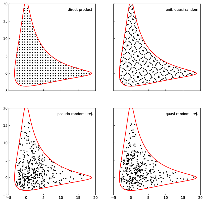
Figure 1: Different methods (see text) to generate $N=350$ grid points for the 2D Morse potential (9) within the cutoff range $V(\mbox{\bf r})<E_{\text{cut}}=11.5$ (indicated by the red contour line). The two top panels show uniformly distributed grids. The non-uniform grids in the two bottom panels follow the distribution, ${\cal P}(\mbox{\bf r})$, defined by Eq. (1) ($\Delta E=1.0$).

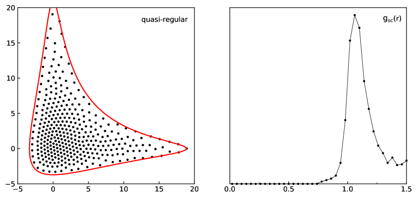
Figure 2: Sampling of the Morse potential (see the caption in Fig. 1) by a quasi-regular grid. The compromise between achieving local regularity and the desired distribution ${\cal P}(\mbox{\bf r})$ is assessed by the sharpness of the peak at $r\sim 1$ in the radial correlation function, $g_{\rm sc}(r)$.

Here, we demonstrate the present method using the 2D distribution function ${\cal P}(\mbox{\bf r})$ arising from the 2D Morse potential (cf. Eq. (1)),

$$V(\mbox{\bf r})=D\sum_{k=1}^{2}\left(e^{-w_{k}\mbox{\bf r}_{k}}-1\right)^{2},$$ (9)

with $E_{\rm cut}=11.5$ and $\Delta E=1.0$, and the Morse parameters: $D=12.0$, $w_{1}=0.2041241$, and $w_{2}=0.18371169$. The appearance of the QRG grid will be compared with the following established grid layouts.

1. Direct-product: A uniformly spaced direct-product grid truncated at $E_{\rm cut}$.

2. Uniform quasi-random: A uniformly distributed 2D low-discrepancy quasi-random sequence (in this work we use the Sobol sequenceSobol’ (1967); Bratley and Fox (1988); Tuffin (1996)), truncated at $E_{\rm cut}$.

3. Uniform pseudo-random+rejection: Starting with a uniformly distributed pseudo-random sequence $\mbox{\bf r}^{(i)}$ in a sufficiently large domain, one retains only the points that satisfy the inequality ${\cal P}\left(\mbox{\bf r}^{(i)}\right)/{\cal P}_{\rm max}>\xi_{i}$, where $\xi_{i}$ is a random number uniformly distributed in the $[0;1]$ interval.

4. Uniform quasi-random+rejection: Same as the above, but $\mbox{\bf r}^{(i)}$ is a 2D Sobol sequence.

We also refer the reader to our recent paper (24) where some of these grids were used to solve the Schrödinger equation with the 2D and 3D Morse potential, and the superiority of QRG was demonstrated.

The results for $N=350$ comparing the five methods are shown in figures 1 and 2. The top two panels in Fig. 1 show two types of uniform grids: a direct-product grid and quasi-random grid. While the quasi-random grid seems to have a somewhat better appearance near the edges, the main drawback of both grid layouts is that too many points are wasted in the region (close to the cutoff line) where the wavefunctions are smooth and less oscillatory. As a consequence, given the fixed total number of points $N=350$, both grids are too sparse in the central region where the wave functions are oscillatory and need a dense grid for an adequate representation. The bottom left panel in Fig. 1 shows a 2D grid generated by a pseudo-random sequence distributed according to the desired distribution function (Eq. (1)). The clustering of grid points and presence of gaps throughout the domain of interest is apparent and is a well known drawback of pseudo-random sampling. The bottom right panel shows the grid obtained by the rejection method from the originally uniform 2D Sobol sequence (i.e., the sequence the beginning part of which appears in the top right panel). Yet, the bottom two panels look very similar. The reason is due to the rejection process. To construct this 350-point grid a large number of points ($\sim$10 000) had to be rejected leading to an almost complete loss of correlations between the remaining points, consequently bringing back the unwanted gaps.

To this end, Fig. 2 shows the QRG result using the same number ($N=350$) of points. The density of the QRG points is consistent with the desired distribution (Eq. (1)) and is locally regular (i.e., locally has uniform spacing between nearest neighbors). The appearance of QRG, at-least visually, is ideal. In addition, the quality of this QRG is confirmed by the radial correlation function $g_{\rm sc}(r)$ which does show a relatively sharp peak at $r\sim 1$.

Calculating the vibrational spectrum of a molecule using the collocation method and internal coordinates.

In this section we briefly describe the collocation method Yang and Peet (1988, 1990) which was also recently used by M&CManzhos and Carrington (2016) to compute the vibrational spectrum of formaldehyde, H2CO. In the latter paper the authors demonstrated that the method could be both improved and simplified further by using the most convenient set of internal coordinates, and evaluating the kinetic energy matrix elements numerically.

Assuming any internal coordinate system $\mbox{\bf r}=(\mbox{\bf r}_{1},...,\mbox{\bf r}_{d})$ that describes a molecule ($d=3N_{\rm atoms}-6$) or its part, the vibrational Hamiltonian reads

$$\widehat{H}=\widehat{T}+V(\mbox{\bf r}),$$ (10)

in which the kinetic energy operator is written using the $3N_{\rm atoms}$ Cartesian coordinates

$$\widehat{T}=-\sum_{i=1}^{3N_{\rm atoms}}-\frac{\hbar^{2}}{2m_{i}}\frac{\partial^{2}}{\partial\mbox{\bf x}_{i}^{2}}.$$ (11)

Consider a set of grid points $\mbox{\bf r}^{(i)}\in\mathbb{R}^{d}$ ($i=1,\cdots,N$), where each point is associated with a basis function, localized in its vicinity. A convenient (albeit not required) choice corresponds to Gaussians,

$$\Phi_{i}(\mbox{\bf r}):=\exp\left[-\left\|\mbox{\bf r}-\mbox{\bf r}^{(i)}\right\|_{{\boldmath\alpha}^{(i)}}^{2}\right]\ \ \ \ (i=1,...,N),$$ (12)

where the norm $\|...\|_{{\boldmath\alpha}^{(i)}}$ is defined by Eq. (5) with the coordinate dependence of the width matrix ${\boldmath\alpha}^{(i)}$ to be specified later.

In the collocation approach one defines a grid of collocation points $\mbox{\bf r}^{(i)}\in\mathbb{R}^{d}$ ($i=1,\cdots,N_{c}$) at which the Schrödinger equation must be satisfied,

$$(\widehat{H}-E)\Psi\left(\mbox{\bf r}^{(j)}\right).$$ (13)

Here, the first $N$ points are set to coincide with the Gaussian centers, and the remaining points are generated separately (see below). By defining the overlap and Hamiltonian matrices,

$$\mbox{\bf S}_{ji}:=\Phi_{i}\left(\mbox{\bf r}^{(j)}\right);\ \ \ \mbox{\bf H}_{ji}:=\widehat{H}\Phi_{i}\left(\mbox{\bf r}^{(j)}\right),$$ (14)

and expanding the eigenfunctions using the Gaussian basis,

$$\Psi(\mbox{\bf r})=\sum_{i=1}^{N}\mbox{\bf c}_{i}\Phi_{i}(\mbox{\bf r}),$$ (15)

we arrive at the rectangular generalized eigenvalue problem,

$$(\mbox{\bf H}-E\mbox{\bf S})\mbox{\bf c}=0$$ (16)

That is, each eigenvalue $E$, Eq. (16) is associated with $N_{c}$ equations and $N$ unknown coefficients $\mbox{\bf c}=(\mbox{\bf c}_{1},...,\mbox{\bf c}_{N})^{\rm T}$. One practical way to solve this (overdetermined) problem is to reduce it to a square $N\times N$ generalized eigenvalue problem as, e.g.,Manzhos and Carrington (2016)

$$(\mbox{\bf S}^{\rm T}\mbox{\bf H}-E\mbox{\bf S}^{\rm T}\mbox{\bf S})\mbox{\bf c}=0.$$ (17)

Note here that in the special case of $N_{c}=N$, one does not need to multiply by $\mbox{\bf S}^{\rm T}$, a step which is not only expensive (scales as $\sim N^{3}$), but also makes the original problem (16) more ill-conditioned. However, given a fixed Gaussian basis, increasing the number of collocation points, $N_{c}$, improves the accuracy of the computed eigenvalues noticeably (see below Fig. 5), while the matrix construction is still comparable or (depending on $N_{c}$) even less expensive than the solution of the (non-symmetric) generalized eigenvalue problem.

In order to avoid very complicated algebra involving internal coordinates, $\mbox{\bf r}=\mbox{\bf r}(\mbox{\bf x})$, the action of the kinetic energy operator (11) on the basis functions at each collocation point, i.e., $\widehat{T}\Phi\left(\mbox{\bf r}^{(j)}\right)$, is evaluated numerically by finite difference in the Cartesian space.Manzhos and Carrington (2016)

Although no integrals involving the potential energy surface (PES) are computed, the method is numerically exact as long as the evaluation of $\nabla^{2}\Phi_{i}(\mbox{\bf r}^{(j)})$ by finite difference is accurate and the basis is large enough.

Here we assume that an optimal distribution function ${\cal P}\left(\mbox{\bf r}^{(i)}\right)$ for the positions of the Gaussian centers is defined using Eq. (1). Again note that we do not need to normalize ${\cal P}\left(\mbox{\bf r}\right)$. The positive-definite matrix ${\boldmath\alpha}$ that appears in the definition of the norm in Eq. (5) is set to be diagonal

$${\boldmath\alpha}:=\mbox{diag}\{1/\Delta r_{k}\}$$ (18)

with $\Delta r_{k}$ defining the range spanned by the Gaussian centers along the $k$-th degree of freedom ($k=1,...,d$).

All the previous experience using DGBsPeet (1989); Meinander and Laane (2001); Glushkov and Wilson (2002); Halverson and Poirier (2012); Dutra, Wickramasinghe, and Garashchuk (2019) suggests that their quality depends very much not only on how the Gaussian centers are distributed but is also very sensitive to the choices of the Gaussian widths, ${\boldmath\alpha}_{i}$. A wrong choice for the latter (e.g., too narrow or too wide) may result in poor approximation of the wavefunctions or ill-conditioned matrices, or both. Clearly, the optimal choice for ${\boldmath\alpha}^{(i)}$ must depend on the local distribution of the Gaussian centers around the $i$-th Gaussian. At the same time, one cannot afford to make the protocol for optimizing the widths matrices ${\boldmath\alpha}^{(i)}$ too elaborate. In the present case, the procedure of choosing ${\boldmath\alpha}^{(i)}$ can be made straightforwardFlynn and Mandelshtam (2019) since the local arrangement of Gaussian centers is the same everywhere, except for a scaling factor. Consequently, we use the following simplified recipe:

$${\boldmath\alpha}^{(i)}:=\frac{b{\boldmath\alpha}}{r_{i,{\rm min}}^{2}},$$ (19)

where $r_{i,{\rm min}}$ is the distance to the nearest neighbor from the i-th point (cf. Eq. (2)) and $b\sim 1$ is the only adjustable parameter.

To this end, we note again that numerical instabilities are often encountered when DGBs are employed, especially when using nonuniform grids. For example, when two grid points appear too close, the corresponding Gaussians become linearly dependent. This in turn leads to a large condition number for both the Hamiltonian and the overlap matrices. A QRG minimizes this very problem as it eliminates the clustering of the grid points. In addition, Eq. (19) assures that all the adjacent Gaussians have similar overlap.

Numerical Details

In our numerical demonstration we consider the four-atom molecule of formaldehyde, H2CO. This choice was motivated by M&CManzhos and Carrington (2016) who used essentially the method formulated in the previous section. We implemented the same PES, i.e., that from Carter,HANDY and Demaison (1997) and the same set of bond-angle internal coordinates ($r_{\rm CO},r_{\rm CH_{1}},r_{\rm CH_{2}},\theta_{1},\theta_{2},\phi$). The difference is in the choice of the points defining the Gaussian centers $\mbox{\bf r}^{(i)}$ and the Gaussian widths matrices ${\boldmath\alpha}^{(i)}$. M&C placed their Gaussians using the same procedure as that implemented to construct the bottom right panel of Fig. 1, i.e. the uniform quasi-random+rejection scheme. In the present case, the Gaussian centers are placed using a QRG. M&C used the same diagonal matrix ${\boldmath\alpha}$ for all Gaussians but the values for its elements were set in a non-transparent fashion which possibly resulted from an additional optimization not explained in the paper. In the present case, the only adjusting parameter for the Gaussian widths was $b$ (cf. Eq. (19)) which was then set to $b=1$ for all the reported results. However, additional calculations (not reported) confirmed that the stability of the results depends on the specific parameters used, meaning further optimization is always possible for a given system. Of note, a larger basis will have a larger region of stability for a given value of $b$, and this stability region decreases as the basis size decreases.

Table 1: The parameters used to construct the QRGs for H2CO. An excessive number of collocation points were used to ensure convergence. Minimal effort was made to optimize these parameters.

data set	QRG10K	QRG15K	QRG20K
$N$	10 000	15 000	20 000
$N_{c}$	500 000	750 000	1 000 000
$E_{\rm cut}$ (cm-1)	15 000	15 000	15 000
$\Delta E$ (cm-1)	3000	5 000	5 000
b	1.0	1.0	1.0

Several calculations were performed using $N=$ 10K, 15K, and 20K (i.e., 10 000, 15 000 and 20 000). The parameters of these calculations are given in Table 1. The grids were constructed according to the following simple protocol. Begin by generating an initial set of points $\{\mbox{\bf r}^{(i)}\}$ ($i=1,...,N$) with Metropolis Monte Carlo using the distribution function ${\cal P}(\mbox{\bf x})$ (Eq. (1)), where each point is selected after 1000 Monte Carlo steps. This grid of points is then used to determine the ranges $\Delta r_{k}$ which define the norm $\|...\|_{\boldmath\alpha}$ (Eq. (5)). In the next step a “greedy simulated annealing minimization” (i.e., the only accepted moves are those resulting in a reduction of the total energy) is applied to the set $\{\mbox{\bf r}^{(i)}\}$ by minimizing the energy functional ${\cal U}(\{\mbox{\bf r}^{(i)}\})$ (Eq. (3)). The convergence of the minimization is monitored by observing the decrease of ${\cal U}(\{\mbox{\bf r}^{(i)}\})$ and by examining the scaled pair correlation function $g_{\rm sc}(r)$ (Eq. (6)). As an example, in Fig. 3 we show $g_{\rm sc}(r)$ for the QRG15K set. The sharp peak at $r\sim 1$ indicates both the local regularity of the grid and its consistency with the given distribution function ${\cal P}(\mbox{\bf x})$.

The additional collocation points were generated using the quasi-random+rejection scheme with the same distribution function ${\cal P}(\mbox{\bf r})$. We note though that switching to the pseudo-random+rejection scheme did not make a noticeable difference (not reported here). Note also that M&C used a quasi-random+rejection sequence for the collocation points, with the first $N$ points in the sequence defining the Gaussian centers. To make sure that insufficient averaging over the collocation grid would not contribute to the error, the maximum number of collocation points was set to a large value, namely, $N_{c,max}=50N$. The convergence with respect to $N_{c}$ was then monitored by solving Eq. (17) for the intermediate values of $N_{c}$. As in Ref. 15 we report the results for the lowest 50 eigenenergies.

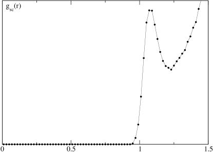
Figure 3: The quality of the 6d QRG constructed for H2CO is assessed using the scaled radial pair correlation function (set QRG15K: $N=15~{}000$, $\Delta E=5~{}000$ cm^-1, $E_{\text{cut}}=15~{}000$ cm^-1 ).

As suggested by M&C here the action of the kinetic energy operator (11) on the basis functions at each collocation point, i.e., $\widehat{T}\Phi_{i}\left(\mbox{\bf r}^{(j)}\right)$, is evaluated numerically by finite difference in the Cartesian space using a five-point stencil. This allows one to avoid very complicated algebra involving the representation of the Laplacian in the bond-angle internal coordinates, and also makes the algorithm very general, i.e., not depending heavily on the choice of the coordinate system.

The generalized eigenvalue problem (17) is not symmetric and hence its eigenvalues are either real or come in complex-conjugated pairs. However, the latter situation indicates poor convergence, i.e., well-converged eigenenergies are always real.

Results

Since the eigenenergies of formaldehyde have already been reported by M&C,Manzhos and Carrington (2016) the purpose of this section is to use this well-established numerical example as a benchmark to further assess the methodology and demonstrate the superiority of a distributed Gaussian basis using a QRG.

There are several factors contributing to the convergence of the computed eigenenergies using the techniques described above. Besides the quality of the Gaussian basis set and the size and extension of the collocation grid we would like to focus first on the numerical errors associated with the evaluation of the Hamiltonian matrix elements. Since the potential energy integrals are avoided, the only numerical error is due to the use of finite difference in the implementation of the Laplacian operator. This simplicity comes with a price, namely: we were unable to achieve very high accuracy, regardless of how elaborate the finite difference scheme was (i.e., either using three-point, five-point or seven-point stencil). For example, Fig. 4 shows the differences in the eigenvalues using the five-point stencil scheme with three different step sizes: 0.01, 0.001, and 0.0001 (mass-scaled coordinates, atomic units). Apparently, the corresponding error increases with the energy from less than 1 cm^-1 for the lowest eigenenergies to about 2 cm^-1 for some of the highest ones. Consequently, one cannot expect the overall error in the eigenenergies to be smaller than the finite-difference error. We noticed though that when the basis is increased, the finite-difference error decreases. Also, in the special case of $N_{c}=N$ (i.e., when the collocation points coincide with the Gaussian centers), the finite-difference error turns out to be negligibly small for either the three-point or five-point stencil. This can be explained by the fact that in this special case the kinetic energy matrix is diagonally-dominated with the diagonal elements obtained by evaluating the second derivatives of the Gaussians at their maxima where the quadratic approximation is excellent if the step size, $\Delta x$, is not too large.

Although the case of $N_{c}=N$ is noticeably faster as it avoids matrix multiplication by $\mbox{\bf S}^{\rm T}$ (cf. Eq. (17)) and, in addition, it does not suffer from the finite-difference error, Fig. 5 clearly demonstrates that using sufficiently large $Nc$ ($\sim 20N$) allows one to substantially reduce the eigenenergy errors compared to the case of $N_{c}=N$.

Table 2: The 50 lowest eigenenergies for H2CO with respect to the ground state energy (first row) following the protocol from Table 1. The final column are the best results from Ref. 15. All results are in cm^-1.

QRG10K	QRG15K	QRG20K	40K(M&C)
5774.24	5774.98	5774.56	5775.3
1166.54	1166.61	1166.75	1166.9
1250.40	1250.44	1250.41	1250.6
1500.47	1500.30	1500.03	1499.7
1746.06	1746.50	1746.28	1747.0
2326.84	2326.88	2326.84	2326.8
2421.62	2421.64	2421.71	2422.0
2497.44	2497.79	2497.56	2498.2
2668.14	2666.90	2666.75	2666.3
2719.18	2719.91	2719.22	2720.6
2775.42	2778.51	2777.80	2780.9
2838.41	2840.30	2840.06	2842.4
2905.07	2905.79	2905.66	2906.0
3000.17	3000.50	3000.02	3001.5
3001.80	3001.35	3000.75	3002.1
3237.85	3239.65	3238.84	3240.3
3468.54	3471.24	3470.93	3472.6
3480.70	3481.20	3480.69	3480.7
3586.04	3586.22	3585.93	3586.4
3674.49	3674.82	3674.64	3675.2
3740.25	3742.34	3741.02	3742.3
3828.80	3826.30	3824.87	3825.5
3887.45	3887.57	3886.80	3887.7
3932.72	3937.00	3936.32	3939.2
3935.10	3937.81	3936.53	3940.3
3989.94	3992.77	3993.11	3995.8
4026.21	4030.62	4028.76	4033.0
4056.47	4058.31	4057.64	4058.2
4079.48	4083.73	4082.39	4085.5
4163.37	4164.65	4164.09	4164.4
4170.13	4166.73	4167.11	4166.3
4193.34	4195.43	4193.66	4196.4
4243.21	4249.72	4247.22	4250.9
4247.25	4251.15	4249.36	4253.4
4331.21	4336.10	4333.88	4337.6
4398.72	4399.54	4398.35	4397.8
4462.42	4468.55	4465.94	4467.3
4495.78	4501.01	4496.02	4507.6
4515.39	4523.12	4521.57	4527.9
4561.92	4569.45	4567.97	4571.6
4618.84	4624.38	4623.11	4624.1
4628.42	4629.58	4627.51	4629.5
4726.54	4732.04	4730.27	4730.4
4729.75	4734.18	4732.22	4734.1
4744.45	4745.66	4744.93	4745.2
4841.30	4843.36	4841.70	4843.5
4924.97	4926.96	4925.87	4926.6
4946.91	4958.41	4954.51	4953.1
4975.21	4980.67	4976.28	4976.7
4982.57	4983.69	4980.56	4983.6

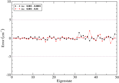
Figure 4: The differences between the eigenenergies (using the QRG15K basis set) when the five-point stencil method is applied while varying the step size $\Delta x$.

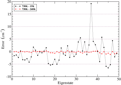
Figure 5: The convergence when using only the Gaussian centers, compared to added collocation points ($N=15~{}000$). In both cases the absolute error is computed against a large iteration ($N_{c}=750~{}000$).

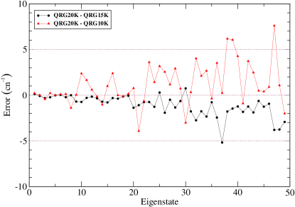
Figure 6: Intrinsic convergence: the eigenenergy differences between QRG10K and QRG15K data sets relative to QRG20K set.

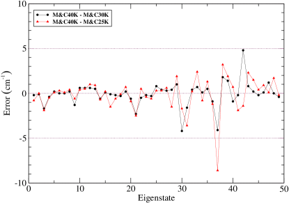
Figure 7: The intrinsic convergence from Ref.15: the eigenenergy differences between the $N$=25K and $N$=30K data sets relative to the largest $N$=40K set and using the collocation grids defined by $N_{c}=10N$

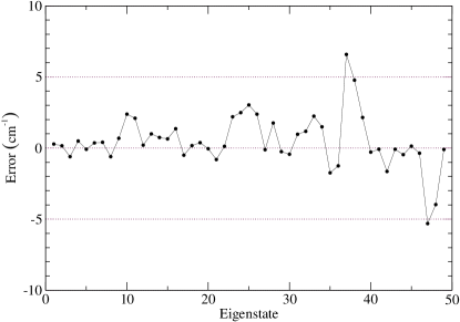
Figure 8: The QRG approach is compared to the largest calculation by M&T,Manzhos and Carrington (2016) i.e. $N$=40K $N_{c}$=400K, through their difference.

To this end, Table 2 presents our results for the first 50 eigenenergies using $N=$10K, 15K, and 20K, together with the most accurate results of M&C using $N=40K$ and $N_{c}=400K$. Overall, the agreement is good between all four sets of calculations and is within a few or several wavenumbers. Figures 6 and 8 visualizes the same information in a graphical form. More specifically, Fig. 6 shows the differences between the eigenenergies of the two pairs of sets, QRG15K-QRG20K and QRG15K-QRG10K; Fig. 7 shows the energy differences between our QRG15K data set and $N$=40K data set from M&C. At the same time, Fig. 8 shows the intrinsic comparison between the three sets reported by M&C using $N$=40K, 30K and 25K. We note that the discrepancies between the latter three data sets are within a range similar to the discrepancies between our data sets.

Based on these comparisons, we can definitely conclude that using a QRG to place the Gaussian basis functions is advantageous compared to the previously used approachManzhos and Carrington (2016) based on the quasi-random + rejection scheme with an improvement of about a factor of 3.

Conclusions

In this paper we revisited our previously introduced method of sampling a general distribution function ${\cal P}(\mbox{\bf r})$ using QRGs.Flynn and Mandelshtam (2019) The revised version is simpler in both the formulation and implementation, very robust, numerically efficient, and has no adjusting parameters. More precisely, due to the special repulsive form of the pair pseudo-potential we were able to avoid the expensive normalization of ${\cal P}(\mbox{\bf r})$ present in the previous version. Moreover, the resulting energy functional is well behaved, i.e., all the local minima are structurally indistinguishable and hence a minimization always results in a correct structure. This was not the case in the previous version of the method in which due to the presence of the attractive term in the pair pseudo-potential a wrong choice in the adjusting parameters could result in holes or even cavities.

The present test calculations of the lowest 50 eigenenergies of formaldehyde demonstrate that a Gaussian basis arranged according to a QRG has superior qualities resulting in about factor of 3-4 reduction in the total number of Gaussians needed to maintain the same accuracy as the previously used quasi-random Gaussian basis.Manzhos and Carrington (2016) Moreover, the regular local arrangement of the Gaussian centers allows one to implement a straightforward procedure for choosing the Gaussian width matrices, which appears to be a non-trivial issue otherwise.

With all the appealing properties and advantages of the present methodology which involves the easy-to-construct efficient and compact Gaussian basis and the following collocation approach to set-up a generalized eigenvalue problem, the only remaining serious drawback of the overall methodology seems to be the consequence of using a non-orthogonal basis and hence the need to deal with the numerical solution of a large generalized eigenvalue problem. Here, two issues need to be addressed: (1) How to solve for the lowest eigenvalues (and eigenvectors) using iterative methods, and (2) parallelization of whatever generalized eigenvalue solver is used. Currently, neither of the two issues seem to have a satisfactory solution.