Ion Heat and Parallel Momentum Transport by Stochastic Magnetic Fields and Turbulence

Abstract

The theory of turbulent transport of parallel momentum and ion heat by the interaction of stochastic magnetic fields and turbulence is presented. Attention is focused on determining the kinetic stress and the compressive energy flux. A critical parameter is identified as the ratio of the turbulent scattering rate to the rate of parallel acoustic dispersion. For the parameter large, the kinetic stress takes the form of a viscous stress. For the parameter small, the quasilinear residual stress is recovered. In practice, the viscous stress is the relevant form, and the quasilinear limit is not observable. This is the principal prediction of this paper. A simple physical picture is developed and shown to recover the results of the detailed analysis.

Keywords: Stochastic Fields, Nonlinear Transport, Magnetohydrodynamics, Fusion Plasma

1 Introduction and Basic Physics

Heat transport, momentum transport, and the formation of shear flows in a stochastic field has long been recognized as a fascinating though complex problem in fusion devices. It is one of the classic ‘paradigm problems’ of magnetic fusion physics and has stimulated the writing of many well-known papers, most notably Rosenbluth et. al 1966 [1] and Rechester & Rosenbluth1978 [2]. In any relevant application, turbulence will co-exist with the stochastic field. This is especially true for L-mode plasmas with resonant magnetic perturbations RMP (before the L-H transition), where the predominantly electrostatic turbulence is strongest just before transition. Hence, studies on stochastic-field-induced effects in presence of strong turbulence is of importance in fusion plasma.

The bulk of the previous works focus on electron thermal transport in a stochastic magnetic field [3, 4, 5, 6]—this is on account of the tiny electron inertia, which is thought to allow long-distance electron streaming along wandering field lines. Then, the more recent awareness of the need to achieve both good confinement and good power handling (and boundary control) has driven a resurgence of interest in the stochastic-field-induced transport problem. Topics of interest include, but are not limited to:

• L-H transition dynamics in a stochastic magnetic field, as produced by (RMPs) [7]. It is now well known that the application of RMPs raises the transition threshold[8, 9, 10, 11, 12, 13, 14, 15] while it ‘stochasticizes’ the edge layer.

• Intrinsic rotation in a stochastic magnetic field, as for the H-mode pedestal torque with RMPs [16, 17, 18, 19, 20].

• Internal transport barrier transitions triggered by magnetic islands[21, 22, 23, 24, 25, 26].

Note that most or all of these phenomena are rooted in ion transport and flow physics—topics rarely associated with the interaction between stochastic magnetic fields and turbulence. This stochastic-field-induced effect was first analytically investigated by Chen et al. [27] which presented a theory of poloidal momentum transport induced by stochastic magnetic fields—the critical rate of stochastic-field-induced scattering $k_{\perp}v_{A}D_{M}$ required to dephase the turbulent poloidal Reynolds stress $\langle\widetilde{u}_{r}\widetilde{u}_{\theta}\rangle$ was calculated; here $k_{\perp}$ is wavenumber perpendicular to the mean field, $v_{A}$ is the Alfvénic speed, $D_{M}=\sum\limits_{k}|\widetilde{b}_{k}|^{2}\pi\delta(k_{\parallel})$ is the magnetic line diffusivity [1], and $\widetilde{u}_{r}$, $\widetilde{u}_{\theta}$ are the perturbed radial and poloidal $E\times B$ flow velocity, respectively. In this paper, we define $\widetilde{b}$ to be a root-mean-square (rms) of normalized fluctuating fields, i.e. $\widetilde{b}\equiv\sqrt{\langle\widetilde{B}^{2}\rangle/B_{0}^{2}}$, where $B_{0}$ is the mean toroidal magnetic field and the bracket average is an ensemble average over symmetry directions, i.e. $\langle\rangle\equiv\frac{1}{2\pi r}\int rd\theta\frac{1}{L_{\parallel}}\int dL_{\parallel}$. Note that the Reynolds stress and force are related to the vorticity flux by the Taylor identity[28], and that the vorticity flux enters $\nabla\cdot J=0$. The Alfvén speed $v_{A}$ then emerges as the speed characteristic of the decorrelation process here. The competition of stochastic field scattering and ambient turbulent decorrelation determines the field fluctuation intensity $\widetilde{b}^{2}$ which can suppress the transition, or equivalently, the increment in power needed to transition in the presence of $\widetilde{b}^{2}$. However, a moment’s consideration of the ion radial force balance equation

$$\langle E_{r}\rangle=\frac{\nabla\langle p_{i}\rangle}{ne}-\langle\mathbb{u}\rangle\times\langle\mathbb{B}\rangle,$$

reminds us that in addition to mean poloidal flow $\langle u_{\theta}\rangle$, the evolution of mean parallel flow $\langle u_{\parallel}\rangle$ and ion pressure $\langle p_{i}\rangle$ should also be revisited in the context of co-existing backgrounds of turbulence and stochastic magnetic fields. To this end, this paper addresses aspects of ion energy and parallel momentum transport induced by the interaction of stochastic fields and turbulence.

Motivated by studies of rotation damping due to ergodic magnetic limiter operation on the TEXT [29], Finn et al. [30] (hereafter referred to as FGC) addressed the ‘stochastic field only’ limit of the problem. The FGC analysis begins from the mean field evolution equation of the parallel flow and pressure —

$$\frac{\partial}{\partial t}\langle u_{\parallel}\rangle+\frac{\partial}{\partial r}\langle\widetilde{u}_{r}\widetilde{u}_{\parallel}\rangle=-\frac{1}{\rho}\frac{\partial}{\partial r}\langle\widetilde{b}_{r},\widetilde{p}\rangle$$ (1)

$$\frac{\partial}{\partial t}\langle p\rangle+\frac{\partial}{\partial r}\langle\widetilde{u}_{r}\widetilde{p}\rangle=-\rho c_{s}^{2}\frac{\partial}{\partial r}\langle\widetilde{b}_{r}\widetilde{u}_{\parallel}\rangle,$$ (2)

where $c_{s}\equiv\sqrt{\gamma p/\rho}$ is the sound speed, $\gamma$ is the adiabatic index, and $\rho$ is the mass density. The familiar advective fluxes of the parallel flow and pressure are ignored. Our goal is then to calculate the kinetic stress ($K\equiv\langle\widetilde{b}_{r}\widetilde{p}\rangle/\rho$) and the compressive energy flux ($H\equiv\rho c_{s}^{2}\langle\widetilde{b}_{r}\widetilde{u}_{\parallel}\rangle$). Note that the divergence of the kinetic stress $\partial_{r}K$ drives mean parallel flow $\langle u_{\parallel}\rangle$ via the pressure gradient along tilted magnetic field lines, while the divergence of the compressive energy flux $\partial_{r}H$ couples field line tilting to compressive heat flow so as to drive energy transport. We note in passing that the kinetic stress has been linked directly to plasma rotation by studies on the Madison Symmetric Torus reverse field pinch [31, 32]. By a combination of probes and polarimetry, Ding et al.[31] demonstrated a clear correlation between the divergence of the measured kinetic stress and the mean $\langle u_{\parallel}\rangle$ profile (see Figure 2. of Ding et al.[31]). This result establishes that stochastic magnetic fields can impact flow dynamics. It is also a compelling insight into the connection among fluctuation measurements, parallel flow dynamics, and momentum transport. Hence, Ding’s study constitutes a rare link between the microscopic and macroscopic facets of the momentum transport problem.

Given the clear resemblance of this problem to aspects of gas dynamics, a natural approach is to cast the analysis in terms of the familiar Riemann variables $u_{\parallel}\pm p$ [33]. A quasilinear analysis then gives an estimate of the relaxation rate for excitation on a perpendicular scale length $l_{\perp}$ as $c_{s}D_{M}/l_{\perp}^{2}$. This rate may be thought of as characteristic of acoustic pulse decorrelation due to propagation along stochastic field lines. However, it should be said that the dynamics here are fundamentally non-diffusive. In particular, the kinetic stress (i.e. $K=-c_{s}D_{M}\partial_{r}\langle p\rangle$) actually is residual stress driven by $\nabla\langle p\rangle$[34]. Likewise, the compressive energy flux (i.e. $H=-c_{s}D_{M}\partial_{r}\langle u_{\parallel}\rangle$) is a non-diffusive contribution to the energy flux driven by $\nabla\langle u_{\parallel}\rangle$—this may be thought of like a pinch. These relations were not presented in FGC. Also, we observe that since basic physics is fundamentally one of a static stochastic field, all key results may be obtained by working directly with $\mathbb{B}\cdot\nabla p=0$ and $\mathbb{B}\cdot\nabla u_{\parallel}=0$.

The analysis discussed so far was quasilinear. FGC obtained expressions for kinetic stress ($K=\langle\widetilde{b}_{r}\widetilde{p}\rangle/\rho$) and compressive energy flux ($H=\rho c_{s}^{2}\langle\widetilde{b}_{r}\widetilde{u}_{\parallel}\rangle$) by computing responses $\widetilde{p}\propto(\delta p/\delta b)\widetilde{b}$, $\widetilde{u}_{\parallel}\propto(\delta u_{\parallel}/\delta b)\widetilde{b}$ and closing the expressions for the kinetic stress and compressional heat flux, yielding both proportional to $D_{M}=\sum\limits_{k}|\widetilde{b}_{k}|^{2}l_{ac}$. Here, $\delta p/\delta b$ and $\delta u_{\parallel}/\delta b$ are responses of pressure and parallel flow to the magnetic perturbation $\widetilde{b}$. The issue is the assumption concerning the physics content of the responses $\delta p/\delta b$ and $\delta u_{\parallel}/\delta b$. To address this turbulent limit, one must calculate the kinetic stress and compressional heat flux in the presence of electrostatic turbulence—i.e. the responses $\delta p/\delta b$ and $\delta u_{\parallel}/\delta b$ must be computed in the presence of a scattering field of electrostatic fluctuations, which we represent as a spectrum of fluctuating $E\times B$ velocities $\langle\widetilde{\mathbb{u}}\;\widetilde{\mathbb{u}}\rangle_{k,\omega}$. As we will show, this makes for a significant and qualitative departure from the quasilinear analysis. Note that this analysis is, in some sense, ‘dual’ to that of Chen et al.[35]. There, the vorticity response $\delta U/\delta\widetilde{u}_{r}$ was calculated in the presence of a prescribed ensemble of $\langle\widetilde{b}^{2}\rangle$ and used to calculate the Reynolds stress, where $U=\nabla_{\perp}^{2}\widetilde{\phi}/B_{0}$ is the $E\times B$ vorticity and $\phi$ denotes the electrical potential. Here, we compute the pressure and parallel flow responses $\delta p/\delta b$ and $\delta u_{\parallel}/\delta b$ in the presence of electrostatic turbulence and use them to calculate the kinetic stress component $\langle\widetilde{b}\widetilde{p}\rangle$. Implicit in both is the assumption that the statistics of the magnetic perturbation field causing the stochasticity are independent of those of the electrostatic perturbation field of the turbulence, i.e. we assume $\langle\widetilde{b}\widetilde{\phi}\rangle=0$. This ansatz eliminates cross-terms from the calculations of fluxes. We discuss this assumption further, later in the paper.

A heuristic but enlightening model of the pressure response $\delta p/\delta b$ is presented here and serves to guide the reader through the subsequent detailed analysis. The parallel flow response $\delta u_{\parallel}/\delta b$ can be estimated in a similar way. Hence, we discuss only $\delta p/\delta b$. Here, it is helpful for the reader to consult Figure 1 and 2. One can ‘pluck’ a magnetic field line by $\widetilde{b}$. Since a mean radial pressure gradient $\partial_{r}\langle p\rangle$ is present, the magnetic perturbation will generate a localized slug of pressure excess-per-length $\widetilde{b}_{r}\partial_{r}\langle p\rangle$. To balance this local pressure excess, there are two possibilities:

• If the rate of turbulent (i.e. viscous) mixing of the parallel flow response is large (i.e. $\nu_{T}/l_{\perp}^{2}>$ other rates), then a turbulent viscosity $\nu_{T}$ will dissipate the parallel flow perturbation $\widetilde{u}_{\parallel}$, produced in response to the magnetic perturbation and pressure slug (see Figure 1). In this case, $\nu_{T}\nabla_{\perp}^{2}\widetilde{u}_{\parallel}\simeq\widetilde{b}_{r}\partial_{r}\langle p\rangle/\rho$, where $\nu_{T}$ is the turbulent viscosity due to the electrostatic turbulence. In this limit, perturbed pressure is replaced by a dynamic balance of the turbulent Reynolds force with the local pressure excess. Here, $\nu_{T}\simeq D_{T}\simeq\int dt^{\prime}\langle\widetilde{u}_{\perp}(0)\widetilde{u}_{\perp}(t^{\prime})\rangle\simeq\langle\widetilde{u}_{\perp}^{2}\rangle\tau_{ac}$, where $\tau_{ac}$ is the autocorrelation time of the electrostatic fluctuation and $D_{T}$ is the turbulent fluid diffusivity.

• If the rate of sound propagation along the perturbed field is large (i.e. $c_{s}/l_{\parallel}>$ other rates), then a pressure gradient will build up along the mean field, so as to cancel the initial imbalance due to the slug (see Figure 2). In this case, $\widetilde{p}c_{s}/l_{\parallel}\simeq-c_{s}\widetilde{b}_{r}\partial_{r}\langle p\rangle$, which leads to the quasilinear result for $\widetilde{p}$ and $K$.

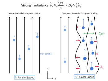
Figure 1: Left: Mean magnetic field in the parallel direction with fluid flow speed. Right: The magnetic field is perturbed by the stochastic field $\widetilde{b}_{r}$. In response to magnetic perturbation and pressure slug, turbulent viscosity $\nu_{T}$ will dissipate the parallel flow perturbation. In Section 3.2, we obtain that the change in mean pressure ($\partial_{x}\langle p\rangle/\rho$) is balanced by turbulent mixing of parallel flow, i.e. $\nabla_{\perp}^{2}\widetilde{u}_{z}$. Blue arrows indicate the change of parallel speed.

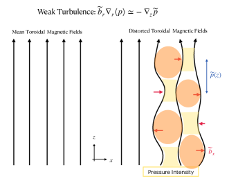
Figure 2: Left: Mean magnetic field in toroidal direction with constant pressure in $z$-direction. Right: The magnetic field is perturbed by the stochastic field $\widetilde{b}_{r}$. In response to magnetic perturbation and pressure slug, the pressure gradient will build up along the mean field. Regions with higher and lower pressure intensity are colored orange and yellow, respectively.

Here, the critical competition (highlighted in Figure 2 and Figure 1) is that between the parallel acoustic transit rate $c_{s}/l_{\parallel}\simeq c_{s}\Delta k_{\parallel}$ and the perpendicular diffusive mixing rate $\simeq\nu_{T}/l_{\perp}^{2}\simeq k_{\perp}^{2}D_{T}$. Hereafter, we take $|k_{\parallel}|\simeq\Delta k_{\parallel}$, where $k_{\parallel}$ may change sign and $\Delta k_{\parallel}$ is always positive. In most relevant cases (i.e. as for drift wave turbulence), $k_{\perp}^{2}D_{T}\simeq\omega>k_{\parallel}c_{s}$, so the dynamic balance regime is relevant. Note that in this regime, the qualitative form of the response to $\widetilde{b}$ differs from the quasilinear case. In particular, a hybrid viscous stress replaces the residual stress and involves turbulent decorrelation resulting from scattering by electrostatic fluctuation. In the weak turbulence regime, we recover perturbed pressure balance. The detailed analysis supports the conclusion derived from heuristics here.

The remainder of this paper is organized as follows. Section 2 presents the models and discusses the quasilinear theory. It also presents the explicit calculation of particle flux and the parallel momentum transport in a steady electric field. Section 3 analyzes the physics of kinetic stress ($K$) and compressive energy flux ($H$), which play important roles in momentum and density evolution. These are calculated in the presence of turbulence. Section 4 discusses the applications of the theory, along with future work.

2 Models and Transport by Static Stochastic Fields

Here, we construct a model for the evolution of density and parallel flow in the presence of stochastic fields in Cartesian (slab) coordinates used in Chen et al. [35] — $x$ is radial, $y$ is poloidal, and $z$ is toroidal direction, in which the mean toroidal field lies (Figure 3).

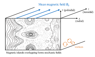
Figure 3: Magnetic fields at the edge of tokamak. RMPs-induced magnetic islands (black lines) lie in radial ($x$) and poloidal ($y$) plane. Mean toroidal field is treading through stochastic fields perpendicular in $z$-direction (blue arrows).

In this 3D system, the stochasticity of magnetic fields, given by a response to an external excitation such as an RMP coil, results from the overlap of magnetic islands located at resonant $\underline{k}\cdot\underline{B}=0$ surfaces [36]. Once overlap occurs, the coherent character of the perturbations is lost, due to finite Kolmogorov-Sinai entropy (i.e. there exists a positive Lyapunov exponent for the field) [37, 38]. Hence, the total magnetic field can be decomposed into the mean toroidal (parallel) field on the $z$-axis plus the stochastic field lying in $x-y$ plane. In this case, we take the magnetic Kubo number [39] to be modest $Ku_{mag}\lesssim 1$ — so mean field theory is valid. This is consistent with reported experimental values of magnetic perturbations $\widetilde{b}$ [40, 41, 42, 43]. We decompose the magnetic fields, magnetic potential, velocities, electric potential, pressure, and density

$$\begin{cases}\text{magnetic fields}&\mathbb{B}=(\widetilde{B}_{x},\widetilde{B}_{y},\;B_{0})\\ \text{potential fields}&\mathbb{A}=(-\frac{1}{2}B_{0}y,\;\frac{1}{2}B_{0}x,\;\widetilde{A}_{(x,y)})\\ \text{velocities}&\mathbb{u}=(\widetilde{u}_{x},\;\langle u_{y}\rangle+\widetilde{u}_{y},\;\langle u_{z}\rangle+\widetilde{u}_{z})\\ \text{electric potential}&\phi=\langle\phi\rangle+\widetilde{\phi}\\ \text{pressure}&p=\langle p\rangle+\widetilde{p}\\ \text{particle density}&n=\langle n\rangle+\widetilde{n}.\end{cases}$$ (3)

Here $\langle u_{y}\rangle$ is the mean poloidal flow, $\langle u_{z}\rangle$ is the mean parallel flow. The tilde $\widetilde{\;\;}$ denotes the perturbations of the mean.

2.1 Non-diffusive Effect for Electron Particle Flux

In this section, we discuss the transport of parallel momentum and particles due to stochastic fields. One aim here is to make contact with and clarify the FGC result [30] as a baseline for later studies of stochastic scattering along with turbulence. Another is to elucidate the contribution to the physics of particle transport in a stochastic magnetic field — i.e. to determine the physical significance of the result. Following FGC, here, we assume an isothermal plasma, so the basic equations reduce to:

$$n\frac{\partial}{\partial t}u_{z}=-c_{s}^{2}\nabla_{z}n,$$ (4)

$$\frac{\partial}{\partial t}n=-n\nabla_{z}u_{z},$$ (5)

where $\nabla_{z}=\nabla_{z}^{(0)}+\widetilde{b}\cdot\nabla_{\perp}$. Then the mean fields $\langle u_{z}\rangle$ and $\langle n\rangle$ evolve according to

$$n_{0}\frac{\partial}{\partial t}\langle u_{z}\rangle=-c_{s}^{2}\frac{\partial}{\partial x}\langle\widetilde{b}_{x}\widetilde{n},\rangle$$ (6)

$$\frac{\partial}{\partial t}\langle n\rangle=-n_{0}\frac{\partial}{\partial x}\langle\widetilde{b}_{x}\widetilde{u}_{z}\rangle,$$ (7)

where $n_{0}$ is a static, uniform background density. Thus, determining the effect of a stochastic field on density evolution (i.e. particle transport) requires a calculation of the flux $\langle\widetilde{b}_{x}\widetilde{u}_{z}\rangle$. Likewise, for the effect on parallel flow, the kinetic stress $c_{s}^{2}\langle\widetilde{b}_{x}\widetilde{n}\rangle$ is needed. The physical interpretation of how the density evolution discussed here is related to the particle flux is discussed at the end of this section.

To calculate $\langle\widetilde{b}_{x}\widetilde{u}_{z}\rangle$ and $\langle\widetilde{b}_{x}\widetilde{n}\rangle$, we proceed by quasilinear theory. Proceeding from Equation (6) and (7), these equations can be written as

$$\frac{\partial}{\partial t}\frac{\widetilde{u}_{z}}{c_{s}}=-c_{s}\nabla_{z}^{(0)}\frac{\widetilde{n}}{n_{0}}-c_{s}\widetilde{b}_{x}\frac{\partial}{\partial x}\frac{\langle n\rangle}{n_{0}},$$ (8)

$$\frac{\partial}{\partial t}\frac{\widetilde{n}}{n_{0}}=-c_{s}\nabla_{z}^{(0)}\frac{\widetilde{u}_{z}}{c_{s}}-c_{s}\widetilde{b}_{x}\frac{\partial}{\partial x}\frac{\langle u_{z}\rangle}{c_{s}}.$$ (9)

We combine Equation (8)$\pm$(9) and obtain the Riemann-like variables $h_{\pm}\equiv\frac{\widetilde{u}_{z}}{c_{s}}\pm\frac{\widetilde{n}}{n_{0}}$, and the Riemann equation

$$\frac{\partial}{\partial t}h_{\pm}\pm c_{s}\frac{\partial}{\partial z}h_{\pm}=-c_{s}\widetilde{b}_{x}\frac{\partial}{\partial x}\frac{\langle n\rangle}{n_{0}}\mp c_{s}\widetilde{b}_{x}\frac{\partial}{\partial x}\frac{\langle u_{z}\rangle}{c_{s}}.$$ (10)

Note that $h_{\pm}$ propagate at $c_{s}$ in opposite directions. Now, the magnetic perturbations here are static, so we can immediately take $\partial_{t}h_{\pm}=0$. No acoustic wave dynamics enters, though the acoustic speed appears in the problem. From Equation (10), we can then immediately write

$$h_{\pm,k}=\mp\int dl[\widetilde{b}_{x}\frac{\partial}{\partial x}\frac{\langle n\rangle}{n_{0}}\pm\widetilde{b}_{x}\frac{\partial}{\partial x}\frac{\langle u_{z}\rangle}{c_{s}}].$$ (11)

Here, $l$ parameterizes the distance along a magnetic field line, and the solution of Equation (10) is affected by integrating along static stochastic field lines. Now, $\widetilde{u}_{z}/c_{s}$ and $\widetilde{n}/n_{0}$ can be recovered noting

$$\frac{\widetilde{u}_{z}}{c_{s}}=(h_{+}+h_{-})/2=-\int dl\widetilde{b}_{x}\frac{\partial}{\partial x}\frac{\langle u_{z}\rangle}{c_{s}},$$ (12)

$$\frac{\widetilde{n}}{n_{0}}=(h_{+}-h_{-})/2=-\int dl\widetilde{b}_{x}\frac{\partial}{\partial x}\frac{\langle n\rangle}{n_{0}},$$ (13)

It then follows that

$$\langle\widetilde{b}_{x}\widetilde{u}_{z}\rangle=-D_{M}\frac{\partial}{\partial x}\langle u_{z}\rangle,$$ (14)

$$\langle\widetilde{b}_{x}\widetilde{n}\rangle=-D_{M}\frac{\partial}{\partial x}\langle n\rangle,$$ (15)

where

$$D_{M}=\int dl\langle\widetilde{b}_{x}(0)\widetilde{b}_{x}(l)\rangle=\langle\widetilde{b}_{x}^{2}\rangle l_{ac},$$ (16)

and $\langle\widetilde{b}_{x}(0)\widetilde{b}_{x}(l)\rangle$ is the magnetic perturbation correlation function, $D_{M}$ is the usual stochastic field diffusivity, and $l_{ac}$ is magnetic perturbation auto-correlation length such that

$$l_{ac}=\frac{1}{\Delta k_{\parallel}}.$$ (17)

The mean field density equation, of this state, is then

$$\frac{\partial}{\partial t}\frac{\langle n\rangle}{n_{0}}=\frac{\partial}{\partial x}c_{s}D_{M}\frac{\partial}{\partial x}\frac{\langle u_{z}\rangle}{c_{s}}.$$ (18)

Note that other physical processes enter the full evolution of density, as discussed below.

Several aspects of these results merit some discussion. First, Equation (14) and (15) are flux-gradient relations with characteristic transport coefficient $c_{s}D_{M}$. Thus the characteristic rate for perturbations on scale $l_{\perp}$ is $1/\tau(l_{\perp})\simeq c_{s}D_{M}/l_{\perp}^{2}$, as noted by FGC. However, the actual fluxes in Equation (14) and (15) are not diffusive, but rather off-diagonal, leading to cross-coupling of $\langle n\rangle$ and $\langle u_{z}\rangle$ evolution. In particular, $\langle\widetilde{b}_{x}\widetilde{u}_{z}\rangle$ yields an off-diagonal convective flux, not particle diffusion. Likewise, $\langle\widetilde{b}_{x}\widetilde{n}\rangle$ contributes a fundamentally non-diffusive residual stress, but not a viscosity. FGC overlooked these points since that their analysis never transformed back from Riemann variables (referred to as Elsässer variables by FGC) to physical variables. We note also that the results of Equation (14) and (15) may be obtained directly from linearizing

$$B\cdot\nabla u_{z}=0$$ (19)

$$B\cdot\nabla n=0$$ (20)

and using $\widetilde{u}_{z}$ and $\widetilde{n}$ to derive the fluxes. The problem is fundamentally static, and no sound wave dynamics is involved.

Equation (18) describes the piece of density evolution in a stochastic magnetic field which is due to $c_{s}\widetilde{b}\cdot\nabla\langle u_{z}\rangle$. A natural question is how is this related to the full particle flux, as it is conventionally understood. FGC refers to the density evolution in this problem as ‘sound wave transport’, yet it is clear that no sound wave dynamics is involved. To clarify this question, we consider electron particle transport in a stochastic magnetic field. Here, we consider the stochastic field as co-existing with plasma current perturbations which generate it, so that Ampère’s law is satisfied. This does not preclude the possibility of external excitation of the stochasticity, as by an RMP. The drift kinetic equation for electrons is

$$\frac{\partial}{\partial t}f+u_{z}\cdot\nabla_{z}f-\frac{E_{\perp}\times\hat{z}}{B_{0}}\cdot\nabla f-\frac{|e|}{m}E_{z}\frac{\partial}{\partial u_{z}}f=C(f),$$ (21)

so that the electron density evolution due to $\widetilde{b}$ effects is determined by

$$\frac{\partial n_{e}}{\partial t}=-n_{0,e}\nabla_{z}u_{z,e},$$ (22)

where $f$ is a general distribution function and $u_{z,e}$ is the parallel electron flow. Then for mean electron density, noting that $\nabla_{z}=\nabla_{z}^{(0)}+\widetilde{b}\cdot\nabla_{\perp}$, it follows that

$$\begin{split}&\frac{\partial\langle n_{e}\rangle}{\partial t}+n_{0,e}\frac{\partial}{\partial x}\langle\widetilde{b}_{x}\widetilde{u}_{z,e}\rangle=0\\ \Rightarrow&\frac{\partial\langle n_{e}\rangle}{\partial t}-\frac{\partial}{\partial x}\frac{\langle\widetilde{b}_{x}\widetilde{J}_{z,e}\rangle}{|e|}=0,\end{split}$$ (23)

where $\widetilde{J}_{z,e}=-\widetilde{u}_{z,e}n_{0,e}|e|$ is electron current density. Note that the divergence of the electron current along tilted field lines (Ampère’s Law) is what determines $\langle n_{e}\rangle$ evolution. Ampère’s Law states

$$-\nabla_{\perp}^{2}A_{z}=\mu_{0}(J_{z,e}+J_{z,i}).$$ (24)

Substitution into Equation (23) gives

$$\frac{\partial\langle n_{e}\rangle}{\partial t}+\frac{1}{\mu_{0}|e|}\frac{\partial}{\partial x}\langle\widetilde{b}_{x}\nabla_{\perp}^{2}\widetilde{A}_{z,e}\rangle+n_{0,i}\frac{\partial}{\partial x}\langle\widetilde{b}_{x}\widetilde{u}_{z,i}\rangle=0.$$ (25)

In the last term on the RHS of Equation (25), we take $u_{z}=u_{z,i}$ the parallel ion flow, consistent with our notation. Using the magnetic Taylor identity [27], we then obtain

$$\frac{\partial\langle n_{e}\rangle}{\partial t}+\frac{\partial}{\partial x}\Gamma_{e,s}=0,$$ (26)

where

$$\Gamma_{e,s}=\frac{-B_{0}}{\mu_{0}|e|}\frac{\partial}{\partial x}\langle\widetilde{b}_{x}\widetilde{b}_{y}\rangle+n_{0}\langle\widetilde{b}_{x}\widetilde{u}_{z}\rangle$$ (27)

is the electron particle flux due to $\widetilde{b}$. Note there are two contributions. The first is the familiar piece due to the divergence of the Maxwell stress [44]. It arises from the flow of current along tilted field lines. The second contribution $\langle\widetilde{b}_{x}\widetilde{u}_{z}\rangle$ studied here is due to ion flow along tilted lines. Note both total and ion current contributions are required to calculate $\partial_{t}\langle n_{e}\rangle$. For the model analyzed here, Equation (14) then gives

$$\Gamma_{e,s}=\frac{-B_{0}}{\mu_{0}|e|}\frac{\partial}{\partial x}\langle\widetilde{b}_{x}\widetilde{b}_{y}\rangle-n_{0}D_{M}\frac{\partial}{\partial x}\langle u_{z}\rangle.$$ (28)

The first term shows that stochastic lines and parallel ion flow gradient drive a net electron particle flux. The second piece adds to the familiar Maxwell force contribution. Note that this stochastic-field-induced particle flux likely is relevant to the phenomenon of ‘RMP pump-out.’ Since the rotation is necessary for stability with RMPs, the $\nabla\langle u_{z}\rangle$-driven flux contribution is of particular relevance. The discussion here clarifies the relations between Equation (18) and the electron particle flux.

3 Calculating the Kinetic Stress and Compressive Energy Flux: Stochastic Fields and Turbulence

In Section 2, we discussed the kinetic stress and compressive energy flux due to stochastic fields. In this section, we consider fluctuating $E\times B$ flow effects. These introduce a relatively fast scattering time scale that enters the response to $\widetilde{b}$. We investigate the evolution of mean parallel flow and that of mean ion pressure (in presence of stochastic fields and turbulence) through the kinetic stress and compressive energy flux, respectively. Consider flow and pressure evolution in the basic model presented in Section 2, we have the parallel acceleration and pressure equations:

$$\frac{\partial}{\partial t}u_{z}+(\mathbb{u}\cdot\nabla)u_{z}=-\frac{1}{\rho}\nabla_{z}p,$$ (29)

$$\frac{\partial}{\partial t}p+(\mathbb{u}\cdot\nabla)p=-\gamma p(\nabla_{z}\cdot\mathbb{u}_{z}),$$ (30)

where $z$ is set in parallel direction, and $x$ and $y$ are set in perpendicular direction. We decompose velocity and pressure as mean and its perturbation such that $\mathbb{u}=\langle\mathbb{u}\rangle+\widetilde{\mathbb{u}}$, $p=\langle p\rangle+\widetilde{p}$. By using mean field theory, we have

$$\frac{\partial}{\partial t}\langle u_{z}\rangle+\frac{\partial}{\partial x}\langle\widetilde{u}_{x}\widetilde{u}_{z}\rangle=-\frac{1}{\rho}\frac{\partial}{\partial x}\langle\widetilde{b}_{x}\widetilde{p}\rangle,$$ (31)

$$\frac{\partial}{\partial t}\langle p\rangle+\frac{\partial}{\partial x}\langle\widetilde{u}_{x}\widetilde{p}\rangle=-\rho c_{s}^{2}\frac{\partial}{\partial x}\langle\widetilde{b}_{x}\widetilde{u}_{z}\rangle.$$ (32)

The right hand side (RHS) of Equation (31) is the divergence of the kinetic stress ($K$) such that

$$-\frac{1}{\rho}\frac{\partial}{\partial x}\langle\widetilde{b}_{x}\widetilde{p}\rangle\equiv-\frac{\partial}{\partial x}K.$$

The kinetic stress $K\equiv\langle\widetilde{b}_{x}\widetilde{p}\rangle/\rho$ is determined by the stochastic magnetic field and the turbulence, as the pressure perturbation $\widetilde{p}$ is scattered by both the drift-wave turbulence and the stochastic field. However, since it is the coherence of $\widetilde{b}_{x}$ and $\widetilde{p}$ that determines $K$, we seek $\widetilde{p}=(\delta p/\delta b)\widetilde{b}$, while including turbulent scattering in $\delta p/\delta b$. Hence, the kinetic stress is derived by considering the $\widetilde{p}$ response to $\widetilde{b}_{x}$ that evolves in the presence of drift wave turbulence. Notice that both the Reynolds stress $\langle\widetilde{u}_{x}\widetilde{u}_{z}\rangle$ and Kinetic stress $\langle\widetilde{p}\widetilde{b}_{r}\rangle/\rho$ in Equation (31) are affected by stochastic magnetic fields. Chen et al. [35] discussed magnetic stochasticity effects on Reynolds stress. Moreover, the RHS of Equation (32) contains the compressive energy flux $H\equiv\rho c_{s}^{2}\langle\widetilde{b}_{x}\widetilde{u}_{z}\rangle$, such that

$$-\rho c_{s}^{2}\frac{\partial}{\partial x}\langle\widetilde{b}_{x}\widetilde{u}_{z}\rangle\equiv-\frac{\partial}{\partial x}H.$$

This compressive energy flux $H$ describes the heat transport effect induced by compression along stochastic magnetic field lines. This effect contributes to the evolution of mean pressure. We do not elaborate further here on the electrostatic Reynolds stress $\langle\widetilde{u}_{x}\widetilde{u}_{z}\rangle$ and the energy flux $\langle\widetilde{u}_{x}\widetilde{p}\rangle$. Note for the former, correlation requires broken symmetry, the mechanisms for which are enumerated in Diamond et al. [20]. Note that details of the broken symmetry are not crucial to the remainder of this paper, so we ignore them hereafter.

We calculate the response of $\widetilde{p}$ and $\widetilde{u}_{z}$ to $\widetilde{b}_{x}$, so as to determine $K$ and $H$. However, we do so in the presence of scattering by drift-wave turbulence. Hence, Equation (29) and Equation (30) yield

$$-i\omega\frac{\widetilde{p}}{\rho c_{s}}+c_{s}ik_{z}\widetilde{u}_{z}+\widetilde{u}_{\perp}\nabla_{\perp}\frac{\widetilde{p}}{\rho c_{s}}=-\widetilde{u}_{x}\frac{\partial}{\partial x}\frac{\langle p\rangle}{\rho c_{s}}-\widetilde{b}_{x}c_{s}\frac{\partial}{\partial x}\langle u_{z}\rangle,$$ (33)

$$-i\omega\widetilde{u}_{z}+c_{s}ik_{z}\frac{\widetilde{p}}{\rho c_{s}}+\widetilde{u}_{\perp}\nabla_{\perp}\widetilde{u}_{z}=-\widetilde{u}_{x}\frac{\partial}{\partial x}\langle u_{z}\rangle-\widetilde{b}_{x}c_{s}\frac{\partial}{\partial x}(\frac{\langle p\rangle}{\rho c_{s}}).$$ (34)

Note that the response to $\widetilde{u}_{x}$ on the RHS is not of interest since we take $\langle\widetilde{b}_{x}\widetilde{u}_{x}\rangle=0$, i.e. we take drift waves and stochastic field uncorrelated, for simplicity. Here, the assumption $\langle\widetilde{b}_{x}\widetilde{u}_{x}\rangle=0$ is based upon the assumed disparity in space-time scales, i.e. $\omega_{\widetilde{b}}\simeq 0$ while $\omega_{\widetilde{u}}\simeq\omega_{*}$, and $l_{\widetilde{b}}<l_{\widetilde{u}}$. Thus, we take the drift wave turbulence as mesoscopic and quasi-Gaussian as usual, with statistics independent of the microscopic $\widetilde{b}_{x}$ (also taken as Gaussian). Further detailed analysis of how non-zero correlation ($\langle\widetilde{b}_{x}\widetilde{u}_{x}\rangle\neq 0$) might develop is given in Cao & Diamond [45]. In particular, that paper shows the development of such correlation is a multi-scale effect and stems from maintaining $\nabla\cdot J=0$ on all scales. The details of this calculation are beyond the scope of this paper. By taking Equation (34) $\pm$ (33), we define the Riemann variables $f_{\pm,k\omega}\equiv\widetilde{u}_{z,k\omega}\pm\widetilde{p}_{k\omega}/\rho c_{s}$ and obtain

$$(-i\omega\pm ic_{s}k_{z}+ik_{\perp}\widetilde{u}_{\perp})f_{\pm,k\omega}=-\widetilde{b}_{x}c_{s}\big{(}\frac{\partial}{\partial x}\frac{\langle p\rangle}{\rho c_{s}}\pm\frac{\partial}{\partial x}\langle u_{z}\rangle\big{)}.$$ (35)

This is the evolution equation for the Riemann response to magnetic perturbation $\widetilde{b}_{x}$. We compute the response of $\widetilde{u}_{z}$ and $\widetilde{p}$ to $\widetilde{b}_{x}$, which is static — i.e. has no time dependence. And $\widetilde{u}_{\perp}$ is taken as stationary. Then, for $\omega\rightarrow 0$, we have:

$$(\pm ic_{s}k_{z}+ik_{\perp}\widetilde{u}_{\perp})f_{\pm,k}=-\widetilde{b}_{x}c_{s}\big{(}\frac{\partial}{\partial x}\frac{\langle p\rangle}{\rho c_{s}}\pm\frac{\partial}{\partial x}\langle u_{z}\rangle\big{)}.$$ (36)

Notice that the $\widetilde{u}_{\perp}\nabla_{\perp}$ operator in Equation (33) and (34) can be expressed as a cumulant scattering effect on a timescale long, compared with the auto-correlation time of drift-wave turbulence $\tau_{ac}$, i.e.

$$\langle\frac{i}{-c_{s}k_{z}\mp\widetilde{u}_{\perp}k_{\perp}}\rangle =\int d\tau e^{-ic_{s}k_{z}\tau}\langle e^{\mp i\widetilde{u}_{\perp}k_{\perp}\int d\tau^{{}^{\prime}}}\rangle$$ (37)

$$=\int d\tau e^{-ic_{s}k_{z}\tau}e^{-\underline{k}_{i}\underline{\underline{D}}_{ij,T}\underline{k}_{j}\tau},$$ (38)

where $D_{ij,T}\equiv\sum\limits_{k}\widetilde{u}_{i,k}\widetilde{u}_{j,k}\tau_{ac}$ is turbulent fluid diffusivity. For perpendicular transport ($i=j=x$ or $y$), we have $D_{T}\equiv\sum\limits_{k}|\widetilde{u}_{\perp,k}|^{2}\tau_{ac}$, which generically is the order of the Gyro-Bohm diffusivity $D_{GB}\sim\rho_{s}^{2}c_{s}/L_{n,\perp}$, as is $\nu_{turb}$. Here, $L_{n,\perp}$ is density scale length. So, we can replace $\widetilde{u}_{\perp}\nabla_{\perp}$ with

$$\widetilde{u}_{\perp}\nabla_{\perp}\equiv-\underline{\nabla}_{\perp}\cdot\underline{\underline{D_{T}}}\cdot\underline{\nabla}_{\perp}.$$ (39)

Hence, Equation (35) become

$$(\pm ic_{s}k_{z}+k_{\perp}^{2}D_{T})f_{\pm,k}=-\widetilde{b}_{x}c_{s}\big{(}\frac{\partial}{\partial x}\frac{\langle p\rangle}{\rho c_{s}}\pm\frac{\partial}{\partial x}\langle u_{z}\rangle\big{)}.$$ (40)

From this equation, we have

$$\begin{split}\frac{\widetilde{p}_{k}}{\rho c_{s}}&=\frac{1}{2}(f_{+,k}-f_{-,k})=\frac{-1}{k_{\perp}^{4}D_{T}^{2}+k_{z}^{2}c_{s}^{2}}\times\\ &\bigg{[}\widetilde{b}_{x,k}c_{s}k_{\perp}^{2}D_{T}\frac{\partial}{\partial x}\langle u_{z}\rangle-ik_{z}c_{s}^{2}\widetilde{b}_{x,k}\frac{\partial}{\partial x}(\frac{\langle p\rangle}{\rho c_{s}})\bigg{]},\end{split}$$ (41)

$$\begin{split}\widetilde{u}_{z,k}&=\frac{1}{2}(f_{+,k}+f_{-,k})=\frac{-1}{k_{\perp}^{4}D_{T}^{2}+k_{z}^{2}c_{s}^{2}}\times\\ &\bigg{[}\widetilde{b}_{x,k}c_{s}k_{\perp}^{2}D_{T}\frac{\partial}{\partial x}(\frac{\langle p\rangle}{\rho c_{s}})-ik_{z}c_{s}^{2}\widetilde{b}_{x,k}\frac{\partial}{\partial x}\langle u_{z}\rangle\bigg{]}.\end{split}$$ (42)

Then, Equation (41) and Equation (42) yield

$$\begin{split}K=\frac{1}{\rho}\langle\widetilde{b}_{x}\widetilde{p}\rangle=\frac{1}{\rho}\sum\limits_{k_{y},k_{z}}|\widetilde{b}_{x,k}|^{2}\frac{-1}{k_{\perp}^{4}D_{T}^{2}+k_{z}^{2}c_{s}^{2}}\\ \bigg{[}\rho c_{s}^{2}k_{\perp}^{2}D_{T}\frac{\partial}{\partial x}\langle u_{z}\rangle-ik_{z}c_{s}^{2}\frac{\partial}{\partial x}\langle p\rangle\bigg{]}.\end{split}$$ (43)

$$\begin{split}H\equiv\rho c_{s}^{2}\langle\widetilde{b}_{x}\widetilde{u}_{z}\rangle=\rho c_{s}^{2}\sum\limits_{k_{y},k_{z}}|\widetilde{b}_{x,k}|^{2}\frac{-1}{k_{\perp}^{4}D_{T}^{2}+k_{z}^{2}c_{s}^{2}}\\ \bigg{[}k_{\perp}^{2}D_{T}\frac{\partial}{\partial x}\frac{\langle p\rangle}{\rho}-ik_{z}c_{s}^{2}\frac{\partial}{\partial x}\langle u_{z}\rangle\bigg{]}.\end{split}$$ (44)

The denominator of the response function $1/(k_{\perp}^{4}D_{T}^{2}+k_{z}^{2}c_{s}^{2})$ can be approximated as $(k_{\perp}^{2}D_{T})^{2}\simeq 1/\tau_{c,k}^{2},$ where $\tau_{c}$ is the decorrelation time due to perpendicular turbulent scattering. The significance of the factor of $i$ in the second term of the source will be apparent when considering reduction to the quasilinear limit (see Section 3.3). Non-zero correlations $\langle\widetilde{b}_{x}\widetilde{u}_{z}\rangle$ and $\langle\widetilde{b}_{x}\widetilde{p}\rangle$, which contribute the kinetic stress $K$ and compressive energy flux $H$, are due to the synergetic effect of the perpendicular turbulent mixing ($k_{\perp}^{2}D_{T}$) and stochastic magnetic field ($|\widetilde{b}_{x}|^{2}$) scattering, via gradients of mean parallel flow $\partial_{x}\langle u_{z}\rangle$ and mean pressure $\partial_{x}\langle p\rangle$. Also, by observing the denominator of the responses, one can notice that $K$ and $H$ can be set by different mechanisms. When $k_{\perp}^{2}D_{T}>k_{z}c_{s}$, the decorrelation due to scattering is stronger than that due to acoustic signal decoherence. For $k_{z}c_{s}>k_{\perp}^{2}D_{T}$, we recover the quasilinear results. These two regimes will be discussed further in Section 3.2 and section 3.3. Finally, note that for $k_{\perp}^{2}D_{T}>k_{\parallel}c_{s}$, the determinant of the transport matrix is positive, so the stability of transport equations (with $K$ and $H$ only) is assured.

3.1 Calculating the flux

In the following Section 3.1, 3.2, and 3.3, we consider the effect of magnetic shear in presence of stochastic fields. We shall calculate the kinetic stress and compressive energy flux in detail. Sheared magnetic field geometry is used to clarify aspects of the competition between acoustic pulse decorrelation at rate $k_{z}c_{s}$ and turbulent scattering, with rate $k_{\perp}^{2}D_{T}$, and its implication for the structure of the fluxes. Attention here is focused on the interplay of different terms in the expressions for $K$ and $H$.

The second term in the denominator of the response function in Equation (43) and (44) can be approximated as $k_{z}^{2}c_{s}^{2}=(k_{y}x/L_{s})^{2}c_{s}^{2},$ where $L_{s}$ the is magnetic shear length such that $1/L_{s}=q^{\prime}r_{0}/q^{2}R_{0}$, $q^{\prime}\equiv dq/dx$, $q$ is the safety factor, and $x$ is the distance from the resonant surface of the perturbation — i.e. $x=r-r_{m,n}$, where $m$, $n$ are the poloidal and toroidal mode numbers, respectively. We decompose Equation (43) into two parts

$$\begin{split}\langle\widetilde{b}_{x}\widetilde{p}\rangle&=\underbrace{\sum\limits_{k_{y},k_{z}}|\widetilde{b}_{x,k}|^{2}\frac{\tau_{c,k}}{1+(k_{y}x/L_{s})^{2}c_{s}^{2}\tau_{c,k}^{2}}\bigg{(}-\rho c_{s}^{2}\frac{\partial}{\partial x}\langle u_{z}\rangle\bigg{)}}_{ⓐ}\\ &+\underbrace{\sum\limits_{k_{y},k_{z}}|\widetilde{b}_{x,k}|^{2}\frac{1}{(k_{\perp}^{2}D_{T})^{2}+k_{z}^{2}c_{s}^{2}}\bigg{(}ik_{z}c_{s}^{2}\frac{\partial}{\partial x}\langle p\rangle\bigg{)}}_{ⓑ}.\end{split}$$ (45)

The spectral sum relevant to this shear effect is $\sum\limits_{k_{y},k_{z}}$. The radial structure is accounted for by the introduction of a box function $F(x/w_{k})$ for the magnetic perturbation intensity, which we further analyze in the following paragraph. We approximate the discrete summation $\sum\limits_{k_{y}k_{z}}$ by a continuous integral:

$$\sum\limits_{k_{y}k_{z}}=\sum\limits_{m,n}=\int dm\int dn.$$ (46)

By using $n=m/q$ and $dn=|m|q^{\prime}dx/q^{2}$, we have

$$\int dm\int dn=\int dm\int dx\frac{|m|}{q^{2}}q^{\prime}=r_{0}\int dk_{y}\int dx\frac{|k_{y}|}{q}\hat{s},$$ (47)

where $\hat{s}=\frac{r_{0}}{q}\frac{dq}{dr}$ is the magnetic shear. Now, we write the magnetic perturbation spectrum $|\widetilde{b}_{x,k}|^{2}$ as

$$|\widetilde{b}_{x,k}|^{2}=CS(k_{y})F(x/w_{k}),$$

where $C$ is a normalization constant, $S(k_{y})$ is the k-spectrum of $\widetilde{b}_{x}$, $F(x/w_{k})$ is the spatial spectrum form factor, and $w_{k}$ is the spatial width of $|\widetilde{b}_{x,k}|^{2}$ (see figure 4) . We assume $|\widetilde{b}_{x,k}|^{2}$ perturbations are densely packed and take the spatial spectrum $F(x/w_{k})$ to be a normalized box function such that $\int dxF(x/w_{k})=1$.

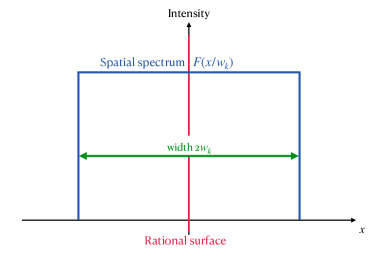
Figure 4: $F(x/w_{k})$ is spatial spectrum for $|\widetilde{b}_{x,k}|^{2}$ in radial direction. Here we define $x=r-r_{m,n}$, where $r_{m,n}$ is the location of a rational surface with mode number $m,\;n$.

Hereafter, we define the intensity of magnetic perturbation $b_{x,0}^{2}$ as

$$b_{x,0}^{2}\equiv\sum\limits_{k_{y}k_{z}}|\widetilde{b}_{x,k}|^{2} =r_{0}\int dk_{y}\int dx\frac{k_{y}\hat{s}}{q}\cdot CS(k_{y})F(x/w_{k}),$$ (48)

$$=C\int dk_{y}\frac{k_{y}r_{0}^{2}q^{\prime}}{q^{2}}S(k_{y})\underbrace{\int dxF(x/w_{k})}_{=1},$$

$$=C\int dk_{y}\frac{k_{y}r_{0}^{2}q^{\prime}}{q^{2}}S(k_{y}).$$

The normalization constant $C$ hence is defined as

$$C\equiv\frac{b_{x,0}^{2}}{\int dk_{y}\frac{k_{y}r_{0}^{2}q^{\prime}}{q^{2}}S(k_{y})}$$ (49)

where $m/r_{0}\equiv k_{y}$, $R_{0}$ and $r_{0}$ are the major and minor radius, respectively. The first term in equation (45) becomes

$$\begin{split}ⓐ&=\sum\limits_{k_{y}k_{z}}|\widetilde{b}_{x,k}|^{2}\frac{\tau_{c,k}}{1+(k_{y}x/L_{s})^{2}c_{s}^{2}\tau_{c,k}^{2}}\bigg{(}-\rho c_{s}^{2}\frac{\partial}{\partial x}\langle u_{z}\rangle\bigg{)}\\ &=\underbrace{C\int dk_{y}\frac{k_{y}r_{0}^{2}q^{\prime}}{q^{2}}S(k_{y})\int dxF(x/w_{k})}_{\sum\limits_{k_{y}k_{z}}|\widetilde{b}_{x,k}|^{2}}\cdot\\ &\;\;\;\frac{\tau_{c,k}}{1+(k_{y}x/L_{s})^{2}c_{s}^{2}\tau_{c,k}^{2}}\bigg{(}-\rho c_{s}^{2}\frac{\partial}{\partial x}\langle u_{z}\rangle\bigg{)}\end{split}$$ (50)

The response function $1/(1+(k_{y}x/L_{s}c_{s}\tau_{c,k})^{2})$ in the equation is the key to understanding the physics of pressure evolution. We define the acoustic width ($x_{s}$) by

$$x_{s}\equiv\frac{L_{s}}{k_{y}c_{s}\tau_{c,k}},$$ (51)

The acoustic width is the value of $x$ for which $k_{z}c_{s}(x)=1/\tau_{c,k}(x)$, where $k_{z}=k_{z}(x)$. So, $x_{s}=L_{s}/k_{y}c_{s}\tau_{c,k}$. Loosely speaking, $x_{s}$ defines the location where the rate of parallel acoustic streaming equals the decorrelation rate. Here $x_{s}$ is analogous to the familiar $x_{i}=\omega L_{s}/k_{y}v_{th,i}$ — the ion Landau resonance point, where $v_{th,ix}$ is the ion thermal speed [46]. The $\tau_{c,k}$ sets the acoustic width — e.g. in strong fluid turbulence (small $\tau_{c}$), $x_{s}$ is large; in weak fluid turbulence, $x_{s}$ is small. Hence, the first term of Equation (45) becomes

$$\begin{split}ⓐ=C\int dk_{y}\frac{k_{y}r_{0}^{2}q^{\prime}}{q^{2}}S(k_{y})\int dxF(x/w_{k})\cdot\\ \frac{\tau_{c,k}}{1+(x/x_{s})^{2}}\big{(}-\rho c_{s}^{2}\frac{\partial}{\partial x}\langle u_{z}\rangle\big{)}\end{split}$$ (52)

For strong turbulence, $\tau_{c,k}$ is small, such that $x_{s}\gg w_{k}$. So $w_{k}$ is the cutoff length in the integral (see Figure 5, green curve). For weak turbulence (i.e. $x_{s}\ll w_{k}$), however, the acoustic width $x_{s}$ is the cutoff length scale (see figure 5, red curve). Let’s consider these two limits.

Figure 5: The integral of spatial spectrum of stochastic field and the response function $\int dxF(x/w_{k})\cdot[1/1+(x/x_{s})^{2}]$. Green and red lines indicate response functions in strong and weak turbulence regime, respectively. For strong turbulence ($x_{s}\gg w_{k}$), $w_{k}$ is the cutoff length in the integral. For weak turbulence ($x_{s}\ll w_{k}$), $x_{s}$ is the cutoff length scale.

3.2 Strong Turbulence

In strong fluid turbulence, we have $x_{s}\gg w_{k}$ ( or $k_{\perp}^{2}D_{T}>k_{z}c_{s}$). Recall in Equation (45), $\langle\widetilde{b}_{x}\widetilde{p}\rangle=ⓐ+ⓑ$. Here, the integral $\int d(x)\frac{F(x/w_{k})}{1+\cancel{x^{2}/x_{s}^{2}}}\simeq 1$. So, the first term in Equation (45) becomes

$$ⓐ\simeq-\rho c_{s}^{2}\sum\limits_{k_{y}k_{z}}|\widetilde{b}_{x,k}|^{2}\tau_{c,k}\frac{\partial}{\partial x}\langle u_{z}\rangle.$$ (53)

The second term in Equation (45), assuming $k_{\perp}^{4}D_{T}^{2}\gg k_{z}^{2}c_{s}^{2}$, becomes small

$$ⓑ=\sum\limits_{k_{y}k_{z}}|\widetilde{b}_{x,k}|^{2}\frac{1}{(k_{\perp}^{2}D_{T})^{2}+k_{z}^{2}c_{s}^{2}}\bigg{(}ik_{z}c_{s}^{2}\frac{\partial}{\partial x}\langle p\rangle\bigg{)}\rightarrow 0,$$ (54)

in the limit $k_{\perp}^{4}D_{T}^{2}\gg k_{z}^{2}c_{s}^{2}$. Derivation details can be found in A. Hence, the kinetic stress can be simplified to

$$\langle\widetilde{b}_{x}\widetilde{p}\rangle\simeq-\rho c_{s}^{2}\sum\limits_{k_{y}k_{z}}|\widetilde{b}_{x,k}|^{2}\tau_{c,k}\frac{\partial}{\partial x}\langle u_{z}\rangle.$$ (55)

This indicates that in the presence of strong scattering, the kinetic stress depends on the electrostatic $\tau_{c,k}$. The kinetic stress hence becomes simply:

$$K\equiv\frac{1}{\rho}\langle\widetilde{b}_{x}\widetilde{p}\rangle\simeq-\sum\limits_{k_{y}k_{z}}|\widetilde{b}_{x,k}|^{2}\tau_{c,k}c_{s}^{2}\frac{\partial}{\partial x}\langle u_{z}\rangle.$$ (56)

From this, we recover a hybrid viscosity produced by stochastic magnetic fields $|\widetilde{b}_{x,k}|^{2}c_{s}^{2}$, with a correlation time set by electrostatic scattering $\tau_{c,k}$. Hence,

$$\begin{split}D_{st}(x)&\equiv\frac{b_{x,0}^{2}\int dk_{y}\frac{k_{y}r_{0}^{2}q^{\prime}}{q^{2}}\tau_{c,k}S(k_{y})c_{s}^{2}}{\int dk_{y}\frac{k_{y}r_{0}^{2}q^{\prime}}{q^{2}}S(k_{y})}\\ &\simeq\sum\limits_{k_{y}k_{z}}|\widetilde{b}_{x,k}|^{2}(x)\frac{c_{s}^{2}}{k_{\perp}^{2}D_{T}},\end{split}$$ (57)

Equation (57) leads us to notice that the combined effects of stochastic fields in the numerator and (electrostatic) turbulent scattering in the denominator together define $D_{st}$. This hybrid turbulent viscosity is the actual diffusivity that describes how the mean flow is scattered by stochastic magnetic fields. The parallel flow evolution equation then becomes

$$\frac{\partial}{\partial t}\langle u_{z}\rangle=-\frac{\partial}{\partial x}\langle\widetilde{u}_{x}\widetilde{u}_{z}\rangle+\frac{\partial}{\partial x}D_{st}(x)\frac{\partial}{\partial x}\langle u_{z}\rangle.$$ (58)

This indicate that the turbulent viscous stress balances $\widetilde{b}_{x}\partial_{x}\langle u_{z}\rangle$.

Similarly, Equation (44) gives the compressive energy flux (H)

$$\begin{split}H(x)&\equiv\rho c_{s}^{2}\langle\widetilde{b}_{x}\widetilde{u}_{z}\rangle\\ &\simeq-c_{s}^{2}\sum\limits_{k_{y}k_{z}}|\widetilde{b}_{x,k}|^{2}\tau_{c,k}\frac{\partial}{\partial x}\langle p\rangle\simeq-D_{st}(x)\frac{\partial}{\partial x}\langle p\rangle.\end{split}$$ (59)

This indicates that the tilting of the magnetic field lines in presence of the pressure gradient (i.e. $\widetilde{b}_{x}\partial\langle p\rangle/\partial x\neq 0$) balances the turbulent diffusion. Notice that Equation (59) also shows that $D_{T}\nabla_{\perp}^{2}\widetilde{u}_{z}\simeq-\sum\limits_{k_{y}k_{z}}\widetilde{b}_{x,k}\partial_{x}(\langle p\rangle/\rho)$. This again indicates that the change in mean pressure ($\partial_{x}\langle p\rangle/\rho$) due to the stochastic fields is balanced by turbulent mixing of parallel flow ($\nabla_{\perp}^{2}\widetilde{u}_{z}$, see Figure 2). The pressure equation now can be written as

$$\frac{\partial}{\partial t}\langle p\rangle=-\frac{\partial}{\partial x}\langle\widetilde{u}_{x}\widetilde{p}\rangle+\frac{\partial}{\partial x}D_{st}(x)\frac{\partial}{\partial x}\langle p\rangle,$$ (60)

again a diffusion equation.

3.3 Weak Turbulence

For weak fluid turbulence, we have $w_{k}\gg x_{s}$ ( or $k_{z}c_{s}>k_{\perp}^{2}D_{T}$). Recall Equation (52)

$$\begin{split}ⓐ=&C\int dk_{y}\frac{k_{y}r_{0}^{2}q^{\prime}}{q^{2}}S(k_{y})\int dxF(x/w_{k})\cdot\\ &\frac{\tau_{c,k}}{1+(x/x_{s})^{2}}\cdot\bigg{(}-\rho c_{s}^{2}\frac{\partial}{\partial x}\langle u_{z}\rangle\bigg{)}.\end{split}$$ (61)

Since in the weak turbulence limit, the cutoff of integral is set by $x_{s}$ and hence $F(x/w_{k})\simeq F(x_{s}/w_{k}\rightarrow 0)$. So, $ⓐ$ is simplified as follows:

$$\begin{split}ⓐ&\simeq\frac{b_{x,0}^{2}\cancel{\int dk_{y}\frac{k_{y}r_{0}^{2}q^{\prime}}{q^{2}}S(k_{y})}}{\cancel{\int dk_{y}\frac{k_{y}r_{0}^{2}q^{\prime}}{q^{2}}S(k_{y})}}\cdot\tau_{c,k}\frac{x_{s}}{w_{k}}F(0)\cdot\\ &\;\;\;\underbrace{\int\limits^{x=x_{s}}_{0}d(x/x_{s})\frac{1}{1+(x/x_{s})^{2}}}_{=arctan(x_{s}/x_{s})=\pi/4}\bigg{(}-\rho c_{s}^{2}\frac{\partial}{\partial x}\langle u_{z}\rangle\bigg{)}\\ &\simeq-b_{x,0}^{2}\tau_{d,k}\frac{x_{s}}{w_{k}}F(0)\frac{\pi}{4}\bigg{(}\rho c_{s}^{2}\frac{\partial}{\partial x}\langle u_{z}\rangle\bigg{)}\end{split}$$ (62)

where $\tau_{d,k}\equiv L_{s}/k_{y}c_{s}w_{k}$ is dispersal timescale of an acoustic wave packet propagating along the stochastic magnetic field. This dispersal timescale $\tau_{d,k}$ defines the width of the acoustic signal ‘cone’. The second term in Equation (45) becomes

$$\begin{split}ⓑ&=\sum\limits_{k_{y}k_{z}}|\widetilde{b}_{x,k}|^{2}\frac{1}{\cancel{(k_{\perp}^{2}D_{T})^{2}}+k_{z}^{2}c_{s}^{2}}\big{(}ik_{z}c_{s}^{2}\frac{\partial}{\partial x}\langle p\rangle\big{)},\\ &\simeq-D_{M}\frac{\partial}{\partial x}\langle p\rangle,\end{split}$$ (63)

where $D_{M}(x)\equiv\sum\limits_{k_{y}k_{z}}|\widetilde{b}_{x,k}|^{2}\tau_{d,k}(x)c_{s}$ is the magnetic diffusivity. Hence, the kinetic stress flux is

$$\langle\widetilde{b}_{x}\widetilde{p}\rangle=-b_{x,0}^{2}\tau_{d,k}F(0)\frac{\pi}{4}\rho c_{s}^{2}\frac{\partial}{\partial x}\langle u_{z}\rangle-D_{M}\frac{\partial}{\partial x}\langle p\rangle.$$ (64)

The first term on the RHS is asymptotically small, so $ⓐ\rightarrow 0$ for $x_{s}/w_{k}\rightarrow 0$ in this limit. The detailed calculation is shown in B. Notice that Equation (81) also shows that $\nabla_{z}\widetilde{p}\simeq-\sum\limits_{k}\widetilde{b}_{x,k}\partial_{x}\langle p\rangle$, by approximating $1/\tau_{d,k}c_{s}$ with operator $\nabla_{z}$. This indicates that the change in mean pressure ($\partial_{x}\langle p\rangle$) due to the stochastic fields is balanced by a parallel pressure gradient ($\nabla_{z}\widetilde{p}$, see Figure 2). The kinetic stress in this limit can be simplified as

$$K(x)\equiv\frac{1}{\rho}\langle\widetilde{b}_{x}\widetilde{p}\rangle\simeq-\frac{1}{\rho}D_{M}(x)\frac{\partial}{\partial x}\langle p\rangle.$$ (65)

Hence, we have the parallel flow evolution

$$\frac{\partial}{\partial t}\langle u_{z}\rangle\simeq-\frac{\partial}{\partial x}\langle\widetilde{u}_{x}\widetilde{u}_{z}\rangle+\frac{\partial}{\partial x}\frac{D_{M}(x)}{\rho}\frac{\partial}{\partial x}\langle p\rangle.$$ (66)

Similarly, we have the compressive energy flux

$$H(x)=\rho c_{s}^{2}\langle\widetilde{b}_{x}\widetilde{u}_{z}\rangle=-\rho c_{s}^{2}D_{M}(x)\frac{\partial}{\partial x}\langle u_{z}\rangle.$$ (67)

Notice that this equation shows the response of mean parallel flow, due to stochastic field tilting ($\widetilde{b}_{x}\partial\langle u_{z}\rangle/\partial x$), is balanced by the parallel flow compression ($\nabla_{\parallel}\widetilde{u}_{z}$), i.e. equivalent to $\underline{B_{z}}\cdot\underline{\nabla}u_{z}=0$ or $\nabla_{\parallel}\widetilde{u}_{z}=-\widetilde{b}_{x}\partial\langle u_{z}\rangle/\partial x$. Hence the pressure equation can be written as

$$\frac{\partial}{\partial t}\langle p\rangle=-\frac{\partial}{\partial x}\langle\widetilde{u}_{x}\widetilde{p}\rangle+\frac{\partial}{\partial x}\rho c_{s}^{2}D_{M}(x)\frac{\partial}{\partial x}\langle u_{z}\rangle.$$ (68)

Equation (65) and (67) indicate that for weak scattering, momentum and energy transport occur only through stochastic fields, with the familiar transport coefficient $c_{s}D_{M}$. There is no dependence on $D_{T}$ for $k_{\perp}^{2}D_{T}\ll k_{z}c_{s}$. This result is equivalent to that in FGC [30]. Note, however, that the key effect for $\langle u_{z}\rangle$ is residual stress; and for $\langle p\rangle$, it is an off-diagonal flux. The comparison of $K$ and $H$ in strong and weak turbulence regime is shown in Table 1.

4 Discussion

In this paper, we develop the theory of ion heat and parallel momentum transport due to stochastic magnetic fields and turbulence. We focus on the kinetic stress ($K$) and the compressional flux ($H$) due to stochastic fields in the presence of (electrostatic) turbulence. The responses $\delta p/\delta b$ and $\delta u_{\parallel}/\delta b$ are calculated by integration over perturbed particle trajectories and then used to close the fluxes. Interestingly, this analysis renders moot one of the deepest questions in stochastic-field-induced transport. Recall that Rechester and Rosenbluth[2] showed that irreversibility requires some means to scatter particles off magnetic field lines, lest they bounce back and undergo no net excursion. Here, ambient cross-field electrostatic scattering supplies this needed effect. Thus, $\delta p/\delta b$ and $\delta u_{\parallel}/\delta b$ should be viewed as statistically averaged nonlinear responses. Here, we posit an ambient ensemble of drift waves, which specifies $\langle\widetilde{u}_{\perp}^{2}\rangle$. The probability distribution functions (PDFs) of $\langle\widetilde{u}_{\perp}^{2}\rangle$ and $\langle\widetilde{b}_{x}^{2}\rangle$ are assumed to be quasi-Gaussian and independent. General results are obtained and shown to recover the dynamic balance limit (viscous dissipation vs. $\widetilde{b}_{x}\partial\langle p\rangle/\partial x$, for $k_{\perp}^{2}D_{T}>k_{z}c_{s}$) and the parallel pressure balance limit ($\nabla_{z}\widetilde{p}$ vs. $\widetilde{b}_{x}\partial\langle p\rangle/\partial x$, for $k_{z}c_{s}>k_{\perp}^{2}D_{T}$), as appropriate. In reality, dynamic balance is the relevant case, and the quasilinear regime is of very limited practical interest. We calculate the explicit form of the turbulent viscous flux and compressive energy flux, and show both are diffusive with a hybrid diffusivity $D_{st}\equiv\sum\limits_{k}|\widetilde{b}_{x,k}^{2}|c_{s}^{2}/k_{\perp}^{2}D_{T}$ — i.e. determined by magnetic fluctuations but with correlation time set by turbulent scattering. The hybrid diffusivity $D_{st}$ is sensitive to the long wavelength content of $|\widetilde{b}_{k}^{2}|$. The analysis is extended to the case of a sheared mean magnetic field. We show that the critical comparison is between the $|\widetilde{b}|^{2}$ spatial spectral width ($w_{k}$) and the acoustic width, i.e. $x_{s}=L_{s}/k_{y}c_{s}\tau_{c,k}$, where $\tau_{c,k}$ is decorrelation time due to perpendicular turbulent scattering.

This paper explores relatively untouched issues, namely the interaction of stochastic magnetic field and turbulence, and how they together drive transport. As such, several of the results merit further discussion. First, while the analysis is in the spirit of a resonance broadening calculation, the basic form of the flux-gradient relation charges with the ratio of $k_{z}c_{s}$ to $k_{\perp}^{2}D_{T}$. Indeed, the kinetic stress changes from a residual stress to a turbulence viscous stress. Also, given that $k_{\perp}^{2}D_{T}\simeq\omega\gg k_{z}c_{s}$, the strong turbulence regime results are surely the relevant ones, and it is unlikely that the pure quasilinear predictions are ever observed. This point is the major prediction of this paper. This outcome is in contrast to the case for the quasilinear predictions for electromagnetic turbulence [47], which are more robust since $\omega$, not $k_{z}c_{s}$, is the relevant base rate there. Second, the sensitivity of the hybrid diffusivity $D_{st}\equiv\sum\limits_{k}|\widetilde{b}_{x,k}^{2}|c_{s}^{2}/k_{\perp}^{2}D_{T}$ to long wavelength (i.e. ‘slow modes’) is interesting and reminiscent of the results of Taylor and McNamara [48]. Further study, including coupling to $E\times B$ shearing, is needed.

Results of this paper are amenable to testing via computer simulations. Such studies would necessarily be non-trivial, as they require simulation of turbulence in stochastic fields. Studies might compare the kinetic stress and compressive energy flux calculated directly from the simulation to the predictions made here. Turbulence intensity could be scanned by varying the deviation from marginality. In this way, one should be able to pass smoothly from the weak turbulence/quasilinear regime ($k_{\perp}^{2}D_{T}\ll k_{z}c_{s}$) to the strong turbulence/nonlinear regime ($k_{\perp}^{2}D_{T}\gg k_{z}c_{s}$), and evaluate scaling trends in both limits.

Several questions and extensions for further study naturally suggest themselves. Magnetic drifts could be included in theory, which could then be used to study the effect of stochastic magnetic fields and turbulence upon geodesic acoustic modes (GAMs) [49, 50, 51, 52, 53]. This topic is of obvious relevance to edge turbulence and transitions. Second, we have assumed throughout the magnetic perturbations and electrostatic turbulence are uncorrelated, i.e. $\langle\widetilde{b}_{x}\widetilde{\phi}\rangle=0$. Recent results, however, indicate that the constraint of $\nabla\cdot J=0$ naturally forces the generation of small scale convective cells by the interaction of long wavelength flows with turbulence. As a consequence, a non-zero $\langle\widetilde{b}_{x}\widetilde{\phi}\rangle$ develops, indicative of small-scale correlations between turbulence and stochastic fields. These may induce novel cross-coupling in the fluxes. Work on this question is ongoing. Finally, since the system studied here essentially is one of gas dynamics in a stochastic field, we note it may have relevance to problems in cosmic ray acceleration and propagation [54]. In those problems, magnetic irregularities are thought to be scatter particles in turbulent environments — similar to the physics discussed in this paper.

Table 1: A comparison of strong and weak turbulent MHD for Kinetic stress and compressive energy flux.

• 	Strong Turbulence	Weak Turbulence
  00 Kinetic Stress
  00 $K\equiv\langle\widetilde{b}_{x}\widetilde{p}\rangle/\rho$	$K=-D_{st}\frac{\partial}{\partial x}\langle u_{z}\rangle$	$K=-D_{M}\frac{\partial}{\partial x}\langle p\rangle$
  Compressive energy flux
  00 $H\equiv\rho c_{s}^{2}\langle\widetilde{b}_{x}\widetilde{u}_{z}\rangle$	$H=-D_{st}\frac{\partial}{\partial x}\langle p\rangle$	$H=-\rho c_{s}^{2}D_{M}\frac{\partial}{\partial x}\langle u_{z}\rangle$

5 DATA AVAILABILITY

The data that support the findings of this study are available from the corresponding author upon reasonable request.

Appendix A Strong Turbulence Limit

In strong fluid turbulence, we have $x_{s}>w_{k}$ (or $k_{\perp}^{2}D_{T}>k_{\parallel}c_{s}$)—$w_{k}$ sets a cut-off for the integral $\int dx$. The first term in Equation (45) becomes

$$\begin{split}ⓐ&=\sum\limits_{k_{y}k_{z}}|\widetilde{b}_{x,k}|^{2}\frac{\tau_{c,k}}{1+(k_{y}x/L_{s})^{2}c_{s}^{2}\tau_{c,k}^{2}}\bigg{(}-\rho c_{s}^{2}\frac{\partial}{\partial x}\langle u_{z}\rangle\bigg{)}\\ &=-C\int dk_{y}\frac{k_{y}r_{0}^{2}q^{\prime}}{q^{2}}\tau_{c,k}S(k_{y})\cdot\int\limits^{x=w_{k}}_{0}dx\frac{F(x/w_{k})}{1+(x/x_{s})^{2}}\bigg{(}\rho c_{s}^{2}\frac{\partial}{\partial x}\langle u_{z}\rangle\bigg{)}\end{split}$$ (69)

We ignore the $(x/x_{s})^{2}$ in the denominator for that in the integration of step function $F(x/w_{k})$, the $1/(1+x^{2}/x_{s}^{2})\rightarrow 1$ (see Figure 5). Hence, in this limit, we obtain

$$\int\limits^{x=w_{k}}_{0}dx\frac{F(x/w_{k})}{1+(x/x_{s})^{2}}\simeq\int\limits^{x=w_{k}}_{0}dxF(x/w_{k})=1$$ (70)

Hence, we have

$$\begin{split}ⓐ&=C\int dk_{y}\frac{k_{y}r_{0}^{2}q^{\prime}}{q^{2}}\tau_{c,k}S(k_{y})\cdot\bigg{(}-\rho c_{s}^{2}\frac{\partial}{\partial x}\langle u_{z}\rangle\bigg{)}\\ &=\frac{b_{x,0}^{2}\cancel{\int dk_{y}\frac{k_{y}r_{0}^{2}q^{\prime}}{q^{2}}S(k_{y})}\tau_{c,k}}{\cancel{\int dk_{y}\frac{k_{y}r_{0}^{2}q^{\prime}}{q^{2}}S(k_{y})}}\bigg{(}-\rho c_{s}^{2}\frac{\partial}{\partial x}\langle u_{z}\rangle\bigg{)}\\ &=-\rho c_{s}^{2}\sum\limits_{k_{y}k_{z}}|\widetilde{b}_{x,k}|^{2}\tau_{c,k}\frac{\partial}{\partial x}\langle u_{z}\rangle\end{split}$$ (71)

Also, the second term in Equation (45) becomes

$$\begin{split}ⓑ&=\sum\limits_{k_{y}k_{z}}|\widetilde{b}_{x,k}|^{2}\frac{1}{(k_{\perp}^{2}D_{T})^{2}+k_{z}^{2}c_{s}^{2}}\bigg{(}ik_{z}c_{s}^{2}\frac{\partial}{\partial x}\langle p\rangle\bigg{)}\\ &=-i\sum\limits_{k_{y}k_{z}}\frac{|\widetilde{b}_{x,k}|^{2}}{k_{z}}(-1+\frac{k_{\perp}^{4}D_{T}^{4}}{k_{\perp}^{4}D_{T}^{4}+k_{z}^{2}c_{s}^{2}})\bigg{(}\frac{\partial}{\partial x}\langle p\rangle\bigg{)},\end{split}$$ (72)

In this limit, we have $k_{\perp}^{2}D_{T}\gg k_{z}^{2}c_{s}^{2}$ such that

$$-1+\frac{k_{\perp}^{4}D_{T}^{4}}{k_{\perp}^{4}D_{T}^{4}+\cancel{k_{z}^{2}c_{s}^{2}}}\simeq 0.$$ (73)

Hence, the second term can be approximated as $ⓑ\simeq 0$, and $\langle\widetilde{b}_{x}\widetilde{p}\rangle$ can be simplified to

$$\langle\widetilde{b}_{x}\widetilde{p}\rangle\simeq-\rho c_{s}^{2}\sum\limits_{k_{y}k_{z}}|\widetilde{b}_{x,k}|^{2}\tau_{c,k}\frac{\partial}{\partial x}\langle u_{z}\rangle.$$ (74)

Appendix B Weak Turbulence Limit

In weak fluid turbulence, we have $w_{k}\gg x_{s}$ ( or $k_{\parallel}c_{s}>k_{\perp}^{2}D_{T}$). The integral in equation (52) becomes

$$\begin{split}ⓐ&=\sum\limits_{k_{y}k_{z}}|\widetilde{b}_{x,k}|^{2}\frac{\tau_{c,k}}{1+(k_{y}x/L_{s})^{2}c_{s}^{2}\tau_{c,k}^{2}}\bigg{(}-\rho c_{s}^{2}\frac{\partial}{\partial x}\langle u_{z}\rangle\bigg{)}\\ &=-C\int dk_{y}\frac{k_{y}r_{0}^{2}q^{\prime}}{q^{2}}S(k_{y})\int dxF(x/w_{k})\frac{\tau_{c,k}}{1+(x/x_{s})^{2}}\cdot\bigg{(}\rho c_{s}^{2}\frac{\partial}{\partial x}\langle u_{z}\rangle\bigg{)}\\ &\simeq-\frac{b_{x,0}^{2}\cancel{\int dk_{y}\frac{k_{y}r_{0}^{2}q^{\prime}}{q^{2}}S(k_{y})}}{\cancel{\int dk_{y}\frac{k_{y}r_{0}^{2}q^{\prime}}{q^{2}}S(k_{y})}}\cdot\tau_{c,k}\frac{x_{s}}{w_{k}}F(0)\cdot\underbrace{\int\limits^{x=x_{s}}_{0}\frac{d(x/x_{s})}{1+(x/x_{s})^{2}}}_{=arctan(x_{s}/x_{s})=\pi/4}\cdot\bigg{(}\rho c_{s}^{2}\frac{\partial}{\partial x}\langle u_{z}\rangle\bigg{)}\end{split}$$ (75)

where $\arctan{(x_{s}/x_{s})}=\arctan{(1)}=\pi/4$ and $\tau_{d,k}\simeq L_{s}/k_{y}c_{s}w_{k}$ is dispersal timescale of acoustic packet propagating along stochastic magnetic fields. Hence,

$$ⓐ\simeq-b_{x,0}^{2}\tau_{d,k}(\frac{x_{s}}{w_{k}})F(0)\frac{\pi}{4}\bigg{(}\rho c_{s}^{2}\frac{\partial}{\partial x}\langle u_{z}\rangle\bigg{)}.$$ (76)

Note that this term scales $\propto x_{s}/w_{k}$, which is asymptotically small as $x_{s}/w_{k}\rightarrow 0$. Then $ⓐ\rightarrow 0$, so the first term is negligible. The second term in equation (52) becomes

$$\begin{split}ⓑ&=\sum\limits_{k_{y}k_{z}}|\widetilde{b}_{x,k}|^{2}\frac{1}{(k_{\perp}^{2}D_{T})^{2}+k_{z}^{2}c_{s}^{2}}\big{(}ik_{z}c_{s}^{2}\frac{\partial}{\partial x}\langle p\rangle\big{)}\\ &=\sum\limits_{k_{y}k_{z}}|\widetilde{b}_{x,k}|^{2}\frac{-i}{k_{z}}(-1+\underbrace{\frac{(k_{\perp}^{2}D_{T})^{2}}{(k_{\perp}^{2}D_{T})^{2}+k_{z}^{2}c_{s}^{2}}}_{=0})\big{(}\frac{\partial}{\partial x}\langle p\rangle\big{)},\end{split}$$ (77)

where the response term is approximated as $i/k_{z}$, since in this limit turbulent scattering is weak—i.e. $k_{\perp}^{2}D_{T}\rightarrow 0$. So, we obtain

$$\begin{split}ⓑ&=\sum\limits_{k_{y}k_{z}}|\widetilde{b}_{x,k}|^{2}\frac{1}{(k_{\perp}^{2}D_{T})^{2}+k_{z}^{2}c_{s}^{2}}\big{(}ik_{z}c_{s}^{2}\frac{\partial}{\partial x}\langle p\rangle\big{)}\\ &\simeq\sum\limits_{k_{y}k_{z}}|\widetilde{b}_{x,k}|^{2}\frac{i}{k_{z}}\frac{\partial}{\partial x}\langle p\rangle.\end{split}$$ (78)

Here, $\sum\limits_{k_{z}}i/k_{z}$ can be approximate as

$$\begin{split}\sum\limits_{k_{z}}\frac{i}{k_{z}-i\delta}&=\sum\limits_{k_{z}}iPV\bigg{[}\frac{1}{k_{z}}\bigg{]}-\pi\delta(k_{z})\\ &=0-\pi\delta(k_{z}),\end{split}$$ (79)

where $PV$ is Cauchy principle value and $\pi\delta(k_{z}c_{s})$ as $\tau_{d,k}$. So, we have

$$\begin{split}ⓑ&\simeq-\sum\limits_{k_{y}k_{z}}|\widetilde{b}_{x,k}|^{2}\pi\delta(k_{z})\frac{\partial}{\partial x}\langle p\rangle\\ &\simeq-D_{M}\frac{\partial}{\partial x}\langle p\rangle,\end{split}$$ (80)

where $D_{M}$ is the magnetic diffusivity. Hence, the kinetic stress flux is

$$\langle\widetilde{b}_{x}\widetilde{p}\rangle=-b_{x,0}^{2}\tau_{d,k}F(0)\frac{\pi}{4}\rho c_{s}^{2}\frac{\partial}{\partial x}\langle u_{z}\rangle-D_{M}\frac{\partial}{\partial x}\langle p\rangle.$$ (81)

The first term on RHS is approximate $ⓐ\simeq 0$ for $F(0)\simeq 0$ in this limit. So, we obtain .

$$\langle\widetilde{b}_{x}\widetilde{p}\rangle=-D_{M}\frac{\partial}{\partial x}\langle p\rangle$$ (82)

in this limit.

References

References

- [1] M.N. Rosenbluth, R.Z. Sagdeev, J.B. Taylor, and G.M. Zaslavski. Destruction of magnetic surfaces by magnetic field irregularities. Nuclear Fusion, 6(4):297–300, dec 1966.
- [2] A. B. Rechester and M. N. Rosenbluth. Electron heat transport in a tokamak with destroyed magnetic surfaces. Phys. Rev. Lett., 40:38–41, Jan 1978.
- [3] I. Joseph, T.E. Evans, A.M. Runov, M.E. Fenstermacher, M. Groth, S.V. Kasilov, C.J. Lasnier, R.A. Moyer, G.D. Porter, M.J. Schaffer, R. Schneider, and J.G. Watkins. Calculation of stochastic thermal transport due to resonant magnetic perturbations in DIII-d. Nuclear Fusion, 48(4):045009, mar 2008.
- [4] O. Schmitz, T. E. Evans, M. E. Fenstermacher, E. A. Unterberg, M. E. Austin, B. D. Bray, N. H. Brooks, H. Frerichs, M. Groth, M. W. Jakubowski, C. J. Lasnier, M. Lehnen, A. W. Leonard, S. Mordijck, R. A. Moyer, T. H. Osborne, D. Reiter, U. Samm, M. J. Schaffer, B. Unterberg, and W. P. West. Resonant pedestal pressure reduction induced by a thermal transport enhancement due to stochastic magnetic boundary layers in high temperature plasmas. Phys. Rev. Lett., 103:165005, Oct 2009.
- [5] K. Ida, M. Yoshinuma, H. Tsuchiya, T. Kobayashi, C. Suzuki, M. Yokoyama, A. Shimizu, K. Nagaoka, S. Inagaki, and K. Itoh. Erratum: Flow damping due to stochastization of the magnetic field. Nature Communications, 6:6531, March 2015.
- [6] Yoshiaki Ohtani, Kenji Tanaka, Hiroe Igami, Katsumi Ida, Yasuhiro Suzuki, Yuki Takemura, Hayato Tsuchiya, Mike Sanders, Mikirou Yoshinuma, Tokihiko Tokuzawa, Ichihiro Yamada, Ryo Yasuhara, Hisamichi Funaba, Mamoru Shoji, Takahiro Bando, and LHD Experimental Group. Effects of core stochastization on particle and momentum transport. Nuclear Fusion, 61(3):034002, feb 2021.
- [7] T. E. Evans, R. A. Moyer, P. R. Thomas, J. G. Watkins, T. H. Osborne, J. A. Boedo, E. J. Doyle, M. E. Fenstermacher, K. H. Finken, R. J. Groebner, M. Groth, J. H. Harris, R. J. La Haye, C. J. Lasnier, S. Masuzaki, N. Ohyabu, D. G. Pretty, T. L. Rhodes, H. Reimerdes, D. L. Rudakov, M. J. Schaffer, G. Wang, and L. Zeng. Suppression of large edge-localized modes in high-confinement diii-d plasmas with a stochastic magnetic boundary. Phys. Rev. Lett., 92:235003, Jun 2004.
- [8] A.W. Leonard, A.M. Howald, A.W. Hyatt, T. Shoji, T. Fujita, M. Miura, N. Suzuki, and S. Tsuji and. Effects of applied error fields on the h-mode power threshold of JFT-2m. Nuclear Fusion, 31(8):1511–1518, aug 1991.
- [9] P. Gohil, T.E. Evans, M.E. Fenstermacher, J.R. Ferron, T.H. Osborne, J.M. Park, O. Schmitz, J.T. Scoville, and E.A. Unterberg. L–h transition studies on DIII-d to determine h-mode access for operational scenarios in ITER. Nuclear Fusion, 51(10):103020, aug 2011.
- [10] S.M. Kaye, R. Maingi, D. Battaglia, R.E. Bell, C.S. Chang, J. Hosea, H. Kugel, B.P. LeBlanc, H. Meyer, G.Y. Park, and J.R. Wilson. L–h threshold studies in NSTX. Nuclear Fusion, 51(11):113019, oct 2011.
- [11] F. Ryter, S.K. Rathgeber, L. Barrera Orte, M. Bernert, G.D. Conway, R. Fischer, T. Happel, B. Kurzan, R.M. McDermott, A. Scarabosio, W. Suttrop, E. Viezzer, M. Willensdorfer, and E. Wolfrum and. Survey of the h-mode power threshold and transition physics studies in ASDEX upgrade. Nuclear Fusion, 53(11):113003, sep 2013.
- [12] S Mordijck, T L Rhodes, L Zeng, E J Doyle, L Schmitz, C Chrystal, T J Strait, and R A Moyer. Effects of resonant magnetic perturbations on turbulence and transport in DIII-d l-mode plasmas. Plasma Physics and Controlled Fusion, 58(1):014003, oct 2015.
- [13] R Scannell, A Kirk, M Carr, J Hawke, S S Henderson, T O’Gorman, A Patel, A Shaw, and A Thornton and. Impact of resonant magnetic perturbations on the l-h transition on MAST. Plasma Physics and Controlled Fusion, 57(7):075013, jun 2015.
- [14] L. Schmitz, D.M. Kriete, R.S. Wilcox, T.L. Rhodes, L. Zeng, Z. Yan, G.R. McKee, T.E. Evans, C. Paz-Soldan, P. Gohil, B. Lyons, C.C. Petty, D. Orlov, and A. Marinoni. L–h transition trigger physics in ITER-similar plasmas with applied n = 3 magnetic perturbations. Nuclear Fusion, 59(12):126010, sep 2019.
- [15] D. M. Kriete, G. R. McKee, L. Schmitz, D. R. Smith, Z. Yan, L. A. Morton, and R. J. Fonck. Effect of magnetic perturbations on turbulence-flow dynamics at the l-h transition on diii-d. Physics of Plasmas, 27(6):062507, 2020.
- [16] J.E Rice, P.T Bonoli, J.A Goetz, M.J Greenwald, I.H Hutchinson, E.S Marmar, M Porkolab, S.M Wolfe, S.J Wukitch, and C.S Chang. Central impurity toroidal rotation in ICRF heated alcator c-mod plasmas. Nuclear Fusion, 39(9):1175–1186, sep 1999.
- [17] J.E Rice, W.D Lee, E.S Marmar, P.T Bonoli, R.S Granetz, M.J Greenwald, A.E Hubbard, I.H Hutchinson, J.H Irby, Y Lin, D Mossessian, J.A Snipes, S.M Wolfe, and S.J Wukitch. Observations of anomalous momentum transport in alcator c-mod plasmas with no momentum input. Nuclear Fusion, 44(3):379–386, feb 2004.
- [18] P.H. Diamond, Y. Kosuga, Ö.D. Gürcan, C.J. McDevitt, T.S. Hahm, N. Fedorczak, J.E. Rice, W.X. Wang, S. Ku, J.M. Kwon, G. Dif-Pradalier, J. Abiteboul, L. Wang, W.H. Ko, Y.J. Shi, K. Ida, W. Solomon, H. Jhang, S.S. Kim, S. Yi, S.H. Ko, Y. Sarazin, R. Singh, and C.S. Chang. An overview of intrinsic torque and momentum transport bifurcations in toroidal plasmas. Nuclear Fusion, 53(10):104019, sep 2013.
- [19] Lu Wang and P. H. Diamond. Gyrokinetic theory of turbulent acceleration of parallel rotation in tokamak plasmas. Phys. Rev. Lett., 110:265006, Jun 2013.
- [20] P.H. Diamond, Y. Kosuga, Ö.D. Gürcan, C.J. McDevitt, T.S. Hahm, N. Fedorczak, J.E. Rice, W.X. Wang, S. Ku, J.M. Kwon, G. Dif-Pradalier, J. Abiteboul, L. Wang, W.H. Ko, Y.J. Shi, K. Ida, W. Solomon, H. Jhang, S.S. Kim, S. Yi, S.H. Ko, Y. Sarazin, R. Singh, and C.S. Chang. An overview of intrinsic torque and momentum transport bifurcations in toroidal plasmas. 53(10):104019, sep 2013.
- [21] Boris V Chirikov. A universal instability of many-dimensional oscillator systems. Physics Reports, 52(5):263–379, 1979.
- [22] K. Ida, N. Ohyabu, T. Morisaki, Y. Nagayama, S. Inagaki, K. Itoh, Y. Liang, K. Narihara, A. Yu. Kostrioukov, B. J. Peterson, K. Tanaka, T. Tokuzawa, K. Kawahata, H. Suzuki, and A. Komori. Observation of plasma flow at the magnetic island in the large helical device. Phys. Rev. Lett., 88:015002, Dec 2001.
- [23] R C Wolf. Internal transport barriers in tokamak plasmas. Plasma Physics and Controlled Fusion, 45(1):R1–R91, nov 2002.
- [24] E Joffrin, C.D Challis, G.D Conway, X Garbet, A Gude, S Günter, N.C Hawkes, T.C Hender, D.F Howell, G.T.A Huysmans, E Lazzaro, P Maget, M Marachek, A.G Peeters, S.D Pinches, S.E Sharapov, and JET-EFDA contributors. Internal transport barrier triggering by rational magnetic flux surfaces in tokamaks. Nuclear Fusion, 43(10):1167–1174, sep 2003.
- [25] K. Ida, M. Yoshinuma, K. Nagaoka, M. Osakabe, S. Morita, M. Goto, M. Yokoyama, H. Funaba, S. Murakami, K. Ikeda, H. Nakano, K. Tsumori, Y. Takeiri, and O. Kaneko and. Spontaneous toroidal rotation driven by the off-diagonal term of momentum and heat transport in the plasma with the ion internal transport barrier in LHD. Nuclear Fusion, 50(6):064007, may 2010.
- [26] K Ida and T Fujita. Internal transport barrier in tokamak and helical plasmas. Plasma Physics and Controlled Fusion, 60(3):033001, jan 2018.
- [27] Chang-Chun Chen and Patrick H. Diamond. Potential vorticity mixing in a tangled magnetic field. The Astrophysical Journal, 892(1):24, mar 2020.
- [28] Geoffrey Ingram Taylor. I. eddy motion in the atmosphere. Philosophical Transactions of the Royal Society of London. Series A, Containing Papers of a Mathematical or Physical Character, 215(523-537):1–26, 1915.
- [29] X. Z. Yang, B. Z. Zhang, A. J. Wootton, P. M. Schoch, B. Richards, D. Baldwin, D. L. Brower, G. G. Castle, R. D. Hazeltine, J. W. Heard, R. L. Hickok, W. L. Li, H. Lin, S. C. McCool, V. J. Simcic, Ch. P. Ritz, and C. X. Yu. The space potential in the tokamak TEXT. Physics of Fluids B: Plasma Physics, 3(12):3448–3461, 1991.
- [30] John M Finn, Parvez N Guzdar, and Alexander A Chernikov. Particle transport and rotation damping due to stochastic magnetic field lines. Physics of Fluids B: Plasma Physics, 4(5):1152–1155, 1992.
- [31] W. X. Ding, L. Lin, D. L. Brower, A. F. Almagri, B. E. Chapman, G. Fiksel, D. J. Den Hartog, and J. S. Sarff. Kinetic stress and intrinsic flow in a toroidal plasma. Phys. Rev. Lett., 110:065008, Feb 2013.
- [32] J.S. Sarff, A.F. Almagri, J.K. Anderson, M. Borchardt, D. Carmody, K. Caspary, B.E. Chapman, D.J. Den Hartog, J. Duff, S. Eilerman, A. Falkowski, C.B. Forest, J.A. Goetz, D.J. Holly, J.-H. Kim, J. King, J. Ko, J. Koliner, S. Kumar, J.D. Lee, D. Liu, R. Magee, K.J. McCollam, M. McGarry, V.V. Mirnov, M.D. Nornberg, P.D. Nonn, S.P. Oliva, E. Parke, J.A. Reusch, J.P. Sauppe, A. Seltzman, C.R. Sovinec, H. Stephens, D. Stone, D. Theucks, M. Thomas, J. Triana, P.W. Terry, J. Waksman, W.F. Bergerson, D.L. Brower, W.X. Ding, L. Lin, D.R. Demers, P. Fimognari, J. Titus, F. Auriemma, S. Cappello, P. Franz, P. Innocente, R. Lorenzini, E. Martines, B. Momo, P. Piovesan, M. Puiatti, M. Spolaore, D. Terranova, P. Zanca, V. Belykh, V.I. Davydenko, P. Deichuli, A.A. Ivanov, S. Polosatkin, N.V. Stupishin, D. Spong, D. Craig, R.W. Harvey, M. Cianciosa, and J.D. Hanson. Overview of results from the MST reversed field pinch experiment. Nuclear Fusion, 53(10):104017, sep 2013.
- [33] Lev Davidovich Landau and E. M. Lifshitz. Fluid mechanics. 1959.
- [34] Ö. D. Gürcan, P. H. Diamond, P. Hennequin, C. J. McDevitt, X. Garbet, and C. Bourdelle. Residual parallel reynolds stress due to turbulence intensity gradient in tokamak plasmas. Physics of Plasmas, 17(11):112309, 2010.
- [35] Chang-Chun Chen, Patrick H. Diamond, Rameswar Singh, and Steven M. Tobias. Potential vorticity transport in weakly and strongly magnetized plasmas. Physics of Plasmas, 28(4):042301, 2021.
- [36] John Wesson and David J Campbell. Tokamaks, volume 149. Oxford university press, 2011.
- [37] Andrei Nikolaevitch Kolmogorov. Entropy per unit time as a metric invariant of automorphisms. In Dokl. Akad. Nauk SSSR, volume 124, pages 754–755, 1959.
- [38] Yakov G Sinai. On the notion of entropy of a dynamical system. In Doklady of Russian Academy of Sciences, volume 124, pages 768–771, 1959.
- [39] Ryogo Kubo. Stochastic liouville equations. Journal of Mathematical Physics, 4(2):174–183, 1963.
- [40] Q Yu, S Günter, K Lackner, A Gude, and M Maraschek. Interactions between neoclassical tearing modes. Nuclear Fusion, 40(12):2031–2039, dec 2000.
- [41] R.C Wolf, W Biel, M.F.M. de Bock, K.H Finken, S Günter, G.M.D Hogeweij, S Jachmich, M.W Jakubowski, R.J.E Jaspers, A Krämer-Flecken, H.R Koslowski, M Lehnen, Y Liang, B Unterberg, S.K Varshney, M. von Hellermann, Q Yu, O Zimmermann, S.S Abdullaev, A.J.H Donné, U Samm, B Schweer, M Tokar, E Westerhof, and the TEXTOR Team. Effect of the dynamic ergodic divertor in the TEXTOR tokamak on MHD stability, plasma rotation and transport. Nuclear Fusion, 45(12):1700–1707, nov 2005.
- [42] Todd E Evans, Richard A Moyer, Keith H Burrell, Max E Fenstermacher, Ilon Joseph, Anthony W Leonard, Thomas H Osborne, Gary D Porter, Michael J Schaffer, Philip B Snyder, et al. Edge stability and transport control with resonant magnetic perturbations in collisionless tokamak plasmas. nature physics, 2(6):419–423, 2006.
- [43] Y. In, J.K. Park, J.M. Jeon, J. Kim, and M. Okabayashi. Extremely low intrinsic non-axisymmetric field in KSTAR and its implications. Nuclear Fusion, 55(4):043004, mar 2015.
- [44] W. X. Ding, D. L. Brower, D. Craig, B. E. Chapman, D. Ennis, G. Fiksel, S. Gangadhara, D. J. Den Hartog, V. V. Mirnov, S. C. Prager, J. S. Sarff, V. Svidzinski, P. W. Terry, and T. Yates. Stochastic magnetic field driven charge transport and zonal flow during magnetic reconnection. Physics of Plasmas, 15(5):055901, 2008.
- [45] Minyun Cao and P.H. Diamond. Physics of Micro-Turbulence in a Stochastic Magnetic Field. In Virtual U.S. Transport Taskforce Workshop, volume Poster, 2021.
- [46] Lev Davidovich Landau. On the vibrations of the electronic plasma. Zh. Eksp. Teor. Fiz., 10:25, 1946.
- [47] Shuitao Peng, Lu Wang, and Yuan Pan. Intrinsic parallel rotation drive by electromagnetic ion temperature gradient turbulence. Nuclear Fusion, 57(3):036003, dec 2016.
- [48] JB Taylor and B McNamara. Plasma diffusion in two dimensions. The Physics of Fluids, 14(7):1492–1499, 1971.
- [49] Niels Winsor, John L. Johnson, and John M. Dawson. Geodesic acoustic waves in hydromagnetic systems. The Physics of Fluids, 11(11):2448–2450, 1968.
- [50] K Itoh, K Hallatschek, and S-I Itoh. Excitation of geodesic acoustic mode in toroidal plasmas. Plasma Physics and Controlled Fusion, 47(3):451–458, feb 2005.
- [51] A V Melnikov, V A Vershkov, L G Eliseev, S A Grashin, A V Gudozhnik, L I Krupnik, S E Lysenko, V A Mavrin, S V Perfilov, D A Shelukhin, S V Soldatov, M V Ufimtsev, A O Urazbaev, G Van Oost, and L G Zimeleva. Investigation of geodesic acoustic mode oscillations in the t-10 tokamak. Plasma Physics and Controlled Fusion, 48(4):S87–S110, mar 2006.
- [52] K. Miki and P. H. Diamond. Role of the geodesic acoustic mode shearing feedback loop in transport bifurcations and turbulence spreading. Physics of Plasmas, 17(3):032309, 2010.
- [53] D. Zarzoso, Y. Sarazin, X. Garbet, R. Dumont, A. Strugarek, J. Abiteboul, T. Cartier-Michaud, G. Dif-Pradalier, Ph. Ghendrih, V. Grandgirard, G. Latu, C. Passeron, and O. Thomine. Impact of energetic-particle-driven geodesic acoustic modes on turbulence. Phys. Rev. Lett., 110:125002, Mar 2013.
- [54] MA Malkov and PH Diamond. Nonlinear dynamics of acoustic instability in a cosmic ray shock precursor and its impact on particle acceleration. The Astrophysical Journal, 692(2):1571, 2009.