XMP gas-rich dwarfs in nearby voids: results of BTA spectroscopy

Abstract

We present the second part of results of the ongoing project aimed at searching for and studying eXtremely Metal-Poor (XMP) – adopted as those with Z_gas $\lesssim$ Z_⊙/30, or with 12+log(O/H) $\lesssim$ 7.21 dex – very gas-rich blue dwarfs in voids. They were first identified in the course of the ’unbiased’ study of the galaxy population in the nearby Lynx–Cancer void. These very rare and unusual galaxies seem to be the best proxies of so-called Very Young Galaxies (VYGs) defined recently in model simulations by Tweed et al. To date, for 16 pre-selected void XMP candidates, using the Big Telescope Alt-azimuth (BTA), the SAO 6-m telescope, we have obtained spectra suitable for the determination of O/H. For majority of the observed galaxies, the principal line [Oiii]$\lambda$4363, used for the direct classical T_e method of O/H determination, is undetected. Therefore, to estimate O/H, we use a new ’strong-lines’ method by Izotov et al. This appears to be the most accurate empirical O/H estimator for the range of 12+log(O/H)$\lesssim$ 7.4–7.5. For objects with higher O/H, we use the semi-empirical method by Izotov & Thuan with our modification accounting for variance of the excitation parameter O₃₂. Six of those 16 candidates are found, with confidence, to be XMP dwarfs. In addition, eight studied galaxies are less metal-poor, with 12+log(O/H)=7.24–7.33, and these can also fall into the category of VYG candidates. Taking into account our recently published work and the previously known (nine prototype galaxies) XMP gas-rich void objects, the new findings increase the number of this type of galaxy known to date to a total of 19.

1 Introduction

This paper is the third in the series devoted to searching for and studying the most metal-poor dwarfs in the nearby voids. In the introductions to the two preceding papers (hereafter referred to as PEPK20 and PKPE20 Pustilnik et al., 2020a, b) we described in detail the previous work and motivation for the ongoing project. Therefore, here we only briefly outline the main points of the earlier searches for the most metal-poor galaxies and the results obtained so far.

The prototype galaxy with the extremely low gas metallicity (Z_gas $\sim$ Z_⊙/30) was discovered about half a century ago (Searle & Sargent, 1972). This is the famous blue compact dwarf galaxy IZw18 (= MRK 116). Being remarkable for its intense star-formation burst, IZw18 remained for a long time the focus of studies in many wavelengths, including the Hubble Space Telescope (HST) study of its resolved stellar population. Early ideas about IZw18 suggested that it is a very young galaxy that formed its first stars several hundred thousand years ago. When its red giant branch (RGB) stars were detected with the help of the HST, its age was increased to at least $\sim$1–2 Gyr. Meanwhile, all the accumulated observational data were reconsidered carefully by Papaderos & Östlin (2012), who found that a large contribution of the overall nebular emission should be accounted for in various photometric parameters. They concluded that however an older stellar population may be present, the major part of the stellar mass in IZw18 formed during the last $\lesssim$1 Gyr. For its companion, IZw18C, the respective age estimate is $\lesssim$0.2 Gyr.

The search for IZw18 analogues has continued since then, mostly among star-forming emission-line galaxies. An important step in this long-lasting process was the discovery of SBS0335–052E and its companion SBS0335–052W, which have similar and lower gas metallicity (Izotov et al., 1990; Pustilnik et al., 1997; Izotov et al., 2009).

Because of the results of massive spectroscopy surveys of faint galaxies, mostly of the Sloan Digital Sky Survey (SDSS; Abazajian et al., 2009; Abolfathi et al., 2018). there has been a substantial advancement in the discovery of eXtremely Metal-Poor (XMP) galaxies. Several groups used the SDSS to search for very metal-poor candidates and to check them with the high-quality follow-up spectroscopy (e.g. Izotov, Thuan, Guseva, 2012; Izotov et al., 2016; Guseva et al., 2017; Sanchez Almeida et al., 2016). In particular, about 300 galaxies were found with the gas metallicity of Z $\lesssim$Z_⊙/10, or 12+log(O/H) $\lesssim$7.7 dex (Izotov et al., 2016). However, the number of galaxies with Z${}_{\rm gas}\lesssim$ Z_⊙/30 found in this way to date does not exceed $\sim$10 objects.

Several alternative methods, based on the colour and morphology selection of XMP candidates from the SDSS image data base, resulted in only singular detections (e.g., Hsyu et al., 2017, 2018).

One of the proposed methods to search for XMP dwarfs was suggested by Pustilnik & Tepliakova (2011) and Pustilnik et al. (2016). It is based on the discovery of the metallicity deficiency (on average, by a factor of $\sim$1.4) of galaxies in voids in comparison with similar objects in typical groups of the Local Volume (LV). It was also found that $\sim$1/3 of the faintest void late-type dwarfs show a strongly reduced gas metallicity. Namely, their values of O/H are lower by a factor of 2–5 relative to those in galaxies of the same luminosity residing in typical groups of the LV (hereafter, the reference sample from Berg et al. (2012)).

Several dwarfs with extremely low gas O/H [12+log(O/H) $\lesssim$ 7.0–7.2], and low or modest star formation rate (SFR), were found in the nearby Lynx–Cancer void at distances of 10–25 Mpc (Pustilnik et al., 2010, 2011, 2016; Hirschauer et al., 2016). The majority of these also show blue colours of the outer parts, consistent with the time since the onset of the main SF episode of $\lesssim$1–3 Gyr, and the extreme gas-mass fractions M_gas/M${}_{\rm bary}\sim$ 0.98–0.99 (e.g. Chengalur, Pustilnik, 2013; , Chengalur et al.2017). However, because they have low luminosities, mostly low surface brightness (LSB) and faint emission lines, the discovery of such galaxies in typical redshift surveys is limited as a result of severe observational selection effects.

This discovery of unusual void dwarfs revealed that they are almost exclusively the least luminous blue LSB galaxies in the Lynx–Cancer void, and encouraged the search for similar objects in other nearby voids, with the help of the recently published ’Nearby Void Galaxies’ (NVG) sample by Pustilnik et al. (2019, hereafter PTM19). This sample was used to separate a group of 60 NVG low-luminosity late-type dwarfs whose properties meant that they resembled prototype gas-rich XMP galaxies (Pustilnik et al., 2020a). For these 60 selected void dwarfs, we performed long-slit spectroscopy to determine their gas O/H. The first part of the spectroscopic results obtained with the Southern African Large Telescope (SALT) was presented in Pustilnik et al. (2020b). Here we present the second part of this study, based on spectroscopy with the Big Telescope Alt-azimuth (BTA), the 6-m telescope of the Special Astrophysical Observatory of Russian Academy of Sciences (SAO RAS).

The rest of this paper is arranged as follows. In Section 2, we describe the observations and data processing. The results of spectral observations of 20 galaxies are presented in Section 3. In Section 4, we discuss the obtained results along with other available information. Finally, in Section 5, we present our conclusions. In Appendices A1 and A2, we present checks of two indirect methods of O/H estimates used in this work. Tables with line intensities, derived physical parameters and oxygen abundances are presented in Appendix B. In Appendix C, (online only), we present the finding charts and plots of the obtained one-dimensional spectra.

Table 1: Journal of BTA spectral observations

	Name	Date	Grating	Exp. time	PA	Galaxy coordinates	$\theta$ (arcsec)	Airmass
	(1)	(2)	(3)	(4)	(5)	(6)	(7)	(8)
1	AGC102728	2019.10.22	1200B	4$\times$1200	99.0	J000021.4+310119	1.5	1.05
	”	2019.10.22	1200R	2$\times$900	99.0	”	1.1	1.06
2	PGC000083	2019.10.22	1200B	4$\times$900	131.0	J000106.5+322241	1.3	1.04
	”	2019.10.28	1200B	2$\times$600	41.5	”	1.5	1.03
	”	2020.01.20	1200B	2$\times$900	59.0	”	1.4	1.37
	”	2020.01.20	1200R	2$\times$900	59.0	”	1.4	1.84
3	PISCESA	2017.11.16	1200B	2$\times$1200	35.5	J001446.0+104847	1.3	1.52
4	AGC411446	2017.09.13	1800R	4$\times$900	98.0	J011003.7–000036	1.7	1.39
	”	2017.11.16	1200B	3$\times$1200	177.0	”	1.2	1.39
5	PISCESB	2017.11.16	1200B	2$\times$1200	35.9	J011911.7+110718	1.0	1.44
6	AGC122400	2019.10.22	1200R	2$\times$600	20.0	J023122.1+254245	1.2	1.19
	”	2020.01.20	1200B	2$\times$900	53.0	”	1.5	1.31
	”	2020.08.19	1200B	3$\times$900	140.0	”	1.2	1.13
7	AGC124609	2019.10.26	1200B	2$\times$900	60.0	J024928.4+344429	1.1	1.10
8	KKH18	2018.01.14	1800R	3$\times$900	235.0	J030305.9+334139	1.9	1.19
9	AGC189201	2019.01.01	1800R	$2\times$900	42.0	J082325.6+175457	3.0	1.33
	”	2019.10.26	1200B	$2\times$900	137.0	”	1.3	1.27
	”	2019.10.26	1200R	$1\times$900	137.0	”	1.3	1.25
	”	2020.01.19	1200B	$3\times$900	173.6	”	1.2	1.33
	”	2020.01.19	1200R	$1\times$600	173.6	”	1.0	1.33
10	J0823+1758	2020.01.19	1200R	$1\times$600	163.0	J082335.0+175813	1.0	1.11
	”	2020.01.20	1200B	$3\times$900	163.0	”	1.5	1.12
	”	2020.01.20	1200R	$2\times$900	163.0	”	1.5	1.33
11	J1012+3946	2018.04.15	1800R	1$\times$900	70.0	J101259.9+394617	1.8	1.11
12	AGC208397	2018.04.15	1800R	3$\times$900	10.0	J103858.1+035227	3.0	1.31
13	AGC239144	2018.04.15	1200B	$4\times$900	109.0	J134908.2+354434	1.2	1.19
	”	2019.01.01	1800R	2$\times$900	120.5	”	3.3	1.07
	”	2020.01.19	1200B	4$\times$900	118.2	”	1.7	1.14
	”	2020.01.19	1200R	2$\times$900	118.2	”	1.7	1.08
14	J1440+3416	2020.01.20	1200B	1$\times$900	119.0	J144431.6+341601	1.1	1.25
	”	2020.05.14	1200B	2$\times$1200	125.6	”	2.6	1.02
	”	2020.05.14	1200R	1$\times$600	125.6	”	2.6	1.02
15	J1444+4242	2017.04.17	1200B	3$\times$1200	41.0	J144449.8+424254	2.4	1.12
16	PGC2081790	2018.04.15	1200B	4$\times$900	11.3	J144744.6+363017	1.3	1.01
17	J1522+4201	2017.09.13	1200B	2$\times$900	62.0	J152255.5+420158	1.4	1.57
18	J2103-0049	2017.09.13	1200B	5$\times$900	05.0	J210347.2–004950	1.7	1.44
19	AGC321307	2017.09.13	1800R	2$\times$900	48.5	J221404.7+254052	1.6	1.14
	”	2017.11.16	1200B	1$\times$1200	23.6	”	1.7	1.07
20	AGC334513	2019.10.28	1200B	2$\times$900	96.0	J234850.4+233527	1.5	1.07
	”	2019.10.28	1200R	2$\times$600	96.0	”	1.5	1.07
	”	2020.01.19	1200B	4$\times$900	49.2	”	1.2	1.47
	”	2020.01.19	1200R	2$\times$900	49.2	”	1.3	1.74
21	J0823+1748	2020.01.19	1200R	$1\times$600	163.0	J082310.6+174826	1.0	1.11
22	AGC322279	2017.09.13	1800R	2$\times$900	167.0	J220316.8+174744	1.4	1.14
23	AGC332939	2017.09.13	1800R	2$\times$900	56.0	J230816.7+315406	1.7	1.11
	”	2017.11.16	1200B	3$\times$1200	25.0	”	1.7	1.03

2 Observations and data reduction

The spectral observations of mainly the Northern part of the XMP candidate sample were conducted with the BTA, which is the SAO 6-m telescope, and the multimode focal reducer SCORPIO (Afanasiev & Moiseev, 2005) in the telescope’s prime focus. In the period from 2017 September to 2019 January (five nights), we used SCORPIO in the original version in the long-slit mode (width of 1.0 arcsec, length of $\sim$6 arcmin). In the period from 2019 October to 2020 August, we observed during seven more nights with the upgraded version of SCORPIO. This upgraded instrument allows us, in particular, to change the pre-installed grisms during observations of the same target, without any time loss. In this period, we used the long-slit mode with a slit width of 1.2 arcsec.

The details of observations for individual galaxies are presented in Table 1, in which we give the galaxy names, the dates of observations, the grisms used, exposure times (in s), position angles of the long slit (PA, in degrees), J2000 coordinates of the target galaxies, seeings $\theta$ (in arcsec) and airmass.

For the main programme, during the dark time, when conditions allowed, we used grism VPHG1200B with the full range of 3650–5450 Å and FWHM = 5.5 Å. The CCD 2K$\times$2K detector was EEV-42-40 with the pixel size of 13.5$\mu$, corresponding to 0.18 arcsec on the detector. We used the binning factor of 2 along the slit. Because our main goal was to obtain the gas metallicity in the observed galaxies, the long slit was oriented close to the current parallactic angle, in order to minimize the effect of atmospheric dispersion (Filippenko, 1982). The emission lines of these spectra were used to derive the electron temperature $T_{\rm e}$ and the oxygen abundance O/H. When it was suitable, during the period since 2019 October, along with grism VPHG1200B we also used grism VPHG1200R. This was done to acquire the spectrum of a studied galaxy in the red (full range 5680–7430 Å, FWHM = 5.5 Å) at exactly the same slit position as for grism VPHG1200B.

For the back-up programme (for cases of ’poor’ seeing and/or Moon time), we used grism VPHG1800R with the range of $\sim$6100–7100 Å and the spectral resolution of FWHM $\sim$ 3.5 Å. Since 2019 October, grism VPHG1800R was unavailable, so for such cases we used grism VPHG1200R. These spectra allowed us to check the coincidence of optical radial velocity with that derived from Hi data for those Hi sources that were identified only because of the close radio and optical positions for the Arecibo Legacy Fast ALFA (ALFALFA) blind Hi survey (Haynes et al., 2018).

Besides, these spectra were used for estimates of the strength of lines [Nii]$\lambda$6584 and doublet [Sii]$\lambda$$\lambda$6716,6731 relative to that of H$\alpha$. This information was subsequently used to rank the observed galaxies, more or less confidently, as XMP candidates for the follow-up observations with grism VPH1200B. A couple of galaxies (numbers 22 and 23 in Tables 1 and 2) were observed at a time when the selection of the void XMP candidates was not finalized. They were identified later as residing outside the nearby voids from PTM19.

The processing of the spectra and the measurement of emission-line fluxes with the use of both IRAF and MIDAS were described in detail in Pustilnik et al. (2016). Below, we describe the main steps of all the procedures used. The standard pipeline included removal of cosmic ray hits, bias subtraction, flat-field correction, wavelength calibration and night-sky background subtraction. By using data of spectrophotometric standards observed on the same nights, all spectra were transformed to absolute fluxes. The individual one-dimensional (1D) spectra of the studied Hii regions were then extracted by summing up without weighting of several rows along the slit. Typically, we extracted 6–12 binned pixels ($\sim$2–4 arcsec).

We note that after the continuum in the 1D spectra is drawn and the line fluxes are measured as described in Pustilnik et al. (2016), we use the iteration procedure from Izotov et al. (1994), which simultaneously determines the extinction coefficient, C(H$\beta$), and the equivalent width of Balmer absorption, EW(abs), in the underlying stellar continuum. See also Sect. 3 for the use of the model continuum for several spectra of E+A type.

The plots of the 1D spectra obtained are presented in Figures S4–S5. in the supplementary data section (online Appendix C). The measured relative fluxes for the presented spectra are available in Appendix B (Tables B1–B7).

As in our previous paper (PKPE20), the majority of the observed candidate XMP dwarfs are very faint and/or of low surface brightness. Thus, it can be a challenge to obtain their independent spectra and to point the slit to the right Hii region. To make it easier to provide independent checks of our data, we provide in Figs S1 and S2 the slit positions for each of the galaxies in our programme overlaid on the galaxy images taken from the data bases of the Dark Energy Camera Legacy Survey (DECaLS; Dey et al., 2019), the Panoramic Survey Telescope & Rapid Response System (PanSTARRS PS1; Flewelling et al., 2020) or the SDSS (Abazajian et al., 2009; Abolfathi et al., 2018). In Fig. S3, we also show the slit positions for three additional observed galaxies that are not in the XMP void candidate list.

Table 2: Candidate XMP dwarfs observed at the BTA and new O/H data. Parameter M(Hi)/L_B is in solar units.

	Name	Galaxy coordinates	Vh	D	Btot	$M_{\rm B}$	M(Hi)/	12+log(O/H)	Notes
			km s-1	(Mpc)	(mag)	(mag)	$L_{\rm B}$
	(1)	(2)	(3)	(4)	(5)	(6)	(7)	(8)	(9)
1	AGC102728	J000021.4+310119	566	8.8	19.40	–10.53	2.44	…	Very faint H$\alpha$
2	PGC000083	J000106.5+322241	542	9.1	17.14	–12.89	3.13	7.15$\pm$0.03 (s,c)	Average of 2 knots
3	PiscesA	J001446.0+104847	235	5.6	17.98	–11.31	2.22	7.26$\pm$0.05 (s,c)
4	AGC411446	J011003.7–000036	1137	15.9	19.58	–11.54	4.80	7.00$\pm$0.05 (s,c)
5	PiscesB	J011911.7+110718	616	8.9	17.63	–12.23	2.80	7.31$\pm$0.05 (s,c)
6	AGC122400	J023122.1+254245	938	15.5	18.48	–12.97	2.27	7.19$\pm$0.12 (s,c)
7	AGC124609	J024928.4+344429	1588	25.0	18.20	–14.10	1.51	7.89$\pm$0.02 (dir)
8	KKH18	J030305.9+334139	210	4.8	16.70	–12.56	0.98	…	I(NII)/I(H$\alpha$)=0.03
9	AGC189201	J082325.6+175457	1475	23.4	19.24	–12.76	3.94	7.31$\pm$0.04 (dir)
10	J0823+1758	J082335.0+175813	1509	23.8	19.49	–12.54	…	7.33$\pm$0.05 (s,c)
11	J1012+3946	J101259.9+394617	1340	21.9	18.32	–12.43	3.80	…	I(NII)/I(H$\alpha$) uncertain
12	AGC208397	J103858.1+035227	763	11.9	19.95	–10.59	5.60	…	I(NII)/I(H$\alpha$)=0.03
13	AGC239144	J134908.2+354434	1366	20.4	19.06	–12.54	3.17	7.25$\pm$0.06 (s,c)	Average of 2 knots
14	AGC249590	J144031.6+341601	1489	21.7	18.45	–13.28	2.67	7.23$\pm$0.05 (s,c)
15	J1444+4242	J144449.8+424254	634	10.9	19.69	–10.54	1.30	7.16$\pm$0.04 (s,c)	Average of 2 knots
16	PGC2081790	J144744.6+363017	1226	18.1	18.04	–13.29	2.11	7.32$\pm$0.04 (s,c)
17	J1522+4201	J152255.5+420158	608	9.8	17.74	–12.31	0.43	7.30$\pm$0.05 (s,c)
18	J2103–0049	J210347.2–004950	1411	17.4	17.44	–14.07	1.30	7.21$\pm$0.04 (s,c)
19	AGC321307	J221404.7+254052	1152	16.2	18.15	–13.27	2.37	7.89$\pm$0.10(mse,c)
20	AGC334513	J234850.4+233527	1662	23.8	18.89	–13.25	3.49	7.24$\pm$0.05 (s,c)
21	J0823+1748	J082310.6+174826	27600	376.4	20.15	–17.86	…	…	Distant I(NII)/I(H$\alpha$)$\sim$0.01
22	AGC322279	J220316.8+174744	1272	17.2	18.39	–12.98	2.37	…	Non-void I(NII)/I(H$\alpha$)=0.19
23	AGC332939	J230816.7+315406	692	10.7	17.18	–13.22	1.61	7.69$\pm$0.06 (dir)	Non-void

3 Results of spectral observations and O/H estimates

Tables with measured line intensities, derived electron temperatures and oxygen abundances are presented in Appendix B (Tables B1–B7).

Because of very low fluxes of emission lines in the observed Hii regions and their low metallicities, the principal faint auroral line [Oiii]$\lambda$4363, used for the determination of the electron temperature, was not detected in the majority of our targets.

The line [Oiii]$\lambda$4363 was reliably detected only in the spectra of three galaxies. For these, O/H was estimated via the direct method and was marked as 12+log(O/H)(T_e). The respective formulae with the most updated atomic data are given in Izotov et al. (2006a). All calculations for the O/H estimate using the direct method are made in a similar way to those in Kniazev et al. (2008) and Pustilnik et al. (2016).

For the 14 remaining objects with detected oxygen lines, we used the two methods described below, which are based on fluxes of the strong oxygen lines: $R_{\mathrm{2}3}$, the flux ratio of the sum of oxygen lines [Oii]$\lambda$3727 and [Oiii]$\lambda\lambda$4959,5007 to the flux of H$\beta$; and the parameter O₃₂, defined here as the flux ratio of [Oiii]$\lambda$5007 to [Oii]$\lambda$3727.

Recently, Izotov et al. (2019b) and Izotov et al. (2021) suggested the variant of an empirical ’strong-lines’ method, which shows small internal scatter for the range of the lowest values of O/H [12+log(O/H) $\lesssim$ 7.5]. This improvement is made by taking into account the dependence of log(O/H) on both parameters, $R_{\mathrm{2}3}$ and O₃₂. The respective relation is:

$$12+log(O/H)=0.950\times log(R_{\mathrm{2}3}-a_{\mathrm{1}}\times O_{\mathrm{3}2})+6.805,$$

where $a_{\mathrm{1}}$ = 0.080 – 0.00078 $\times O_{\mathrm{3}2}$. While the strong-lines method is suitable only for the lowest metallicities, as the authors show, for this range, it provides a low internal scatter of $\sim$0.05 dex. We mark O/H estimated with this strong-lines method as 12+log(O/H)(s). The above relation empirically accounts for the large scatter in the ionization parameter $U$ in various Hii regions. This leads to a reduction in the relatively large internal scatter inherent to the other methods based on strong oxygen lines.

For 13 of 14 void objects with detected strong oxygen lines, but without the [Oiii]$\lambda$4363 line, the line ratios are indicative of that low level of O/H. Hence, for those objects, we used the strong-lines method of Izotov et al. (2019b) and its recent slightly modified version (Izotov et al., 2021) as the most reliable. We also perform our own analysis in Appendix A1, illustrated in Figure 2, addressing both the issues of its small offset relative to O/H(dir) and its internal scatter.

For one of the void galaxies, J2214+2540, its strong oxygen lines indicate 12+log(O/H) $>$ 7.5 and hence other methods of estimating O/H are needed. A so-called semi-empirical (hereafter, se) method by Izotov & Thuan (2007) is based on a correlation between T_e and parameter $R_{\mathrm{2}3}$. The functional relation between the two variables was fitted based on calculations for the grid of Hii region models in a paper by Stasinska & Izotov (2003). The se method first calculates the empirical estimate of T_e from the measured $R_{\mathrm{2}3}$ and then uses this T_e similar to the classical direct method. This method was checked and calibrated in particular by Izotov & Thuan (2007) and Pustilnik et al. (2016). Its internal scatter was estimated as rms $\sim$0.07–0.08 dex. The method is applicable for 12+log(O/H) $\lesssim$ 7.9.

In the course of the review process for this paper, it was drawn to our attention that for some galaxies with a well-measured flux of [Oiii]$\lambda$4363 and the related good accuracy estimate of the electron temperature T_e in the O⁺⁺ zone, the difference between T_e(dir) and T_e(R₂₃) may reach several thousand K. This in turn might lead to a bias in the estimate of O/H via the se method.

We address this issue in more detail in Appendix A.2 and then apply the results of the modified semi-empirical method (hereafter mse) to the current observations. This mse method will also be applied to our earlier data for void galaxies with 12+log(O/H) $>$ 7.5, when we will summarize all their metallicity data.

For a few of the observed galaxies, Balmer absorption lines were clearly visible in the blue-UV range. We modeled their underlying continuum with the ULySS package (Koleva et al., 2009). This model continuum fitted Balmer absorption lines, and thus corrected to a first approximation the flux of H$\beta$ emission. For these objects, the EW(abs) derived in the next step via iterations, as described above with the procedure from Izotov et al. (1994), relates in fact to the residual EW(abs), which is already mainly accounted for by the ULySS fitting (e.g., in galaxies J2103–0049 and J2214+2540).

In Table 2 we present the following parameters. Columns 1 and 2 give the name and J2000 RA and declination of the galaxy. In column 3, we give the heliocentric velocities as adopted from HyperLEDA data base. For J0823+1758 and J0823+1748, we present radial velocities which were first measured by us (see Section 4.1 for details). The distances in Mpc (column 4) derived from the HST data via the tip of the RGB (TRGB) for four galaxies are taken from HyperLEDA; for the remaining 16 galaxies, they are taken from our NVG catalogue (PTM19) based on the velocity field model by Tully et al. (2008). In columns 5 and 6, we give the total apparent and respective absolute blue magnitudes. The latter are calculated from the apparent magnitudes and the adopted distances, taking into account the Galaxy extinction from Schlafly & Finkbeiner (2011).

The apparent blue magnitudes B_tot were estimated by us via measurements of their $g,r$ magnitudes if their images were available in the above-mentioned public data bases. Then/ these $g,r$ magnitudes were transformed to the $B$ band via the relation of Lupton et al. (2005). In the remaining cases, we took B_tot from HyperLEDA. In column 7, we also give the ratio of hydrogen mass to blue luminosity M(Hi)/L_B, in solar units. In column 8, the adopted value of 12+log(O/H) is presented as derived in this paper. In column 9, we give some notes.

Tables with measured line intensities, derived electron temperatures and oxygen abundances are presented in Appendix B. Besides 12+log(O/H)(dir), we show 12+log(O/H)(s,c), 12+log(O/H)(mse,c) and 12+log(O/H)(se,c). In Table 2, for the range of 12+log(O/H) $\lesssim$ 7.4 dex, when the strong-lines method is applicable, we adopted the value of 12+log(O/H) (s,c). As shown in Appendices A.1 and A.2, this estimate has a significantly smaller scatter in comparison to those of 12+log(O/H) (mse,c) and 12+log(O/H) (se,c).

4 Discussion

4.1 Notes on individual galaxies

For some of our observed XMP dwarf candidates, it is worth giving additional information or comments.

4.1.1 AGC102728 = J0000+3101

Only a faint H$\alpha$ line was seen in one of the positions along the long slit. This galaxy is resolved into individual stars at the HST images. Tikhonov & Galazutdinova (2019) derived its distance of 8.84$\pm$0.68 Mpc based on the TRGB method. An alternative TRGB distance for this galaxy of D=12.4 Mpc was recently derived in McQuinn et al. (2021). In the colour HST image, several faint red galaxies are seen in the surroundings of this galaxy; these could belong to a distant group or a cluster. Our slit position crossed one of these galaxies projected on to the body of AGC102728. A clear emission line was detected at $\lambda$6863 Å corresponding to a redshifted H$\alpha$ line with $z$ = 0.04571.

4.1.2 PiscesA = J0014+1048

This galaxy was included, among others, in the list of about 80 candidate low-metallicity dwarfs selected on their morphological and colour properties by James et al. (2017). However, for two different positions of the long slit, these authors did not detect emission lines in their spectra. As our results show, the reason is that PiscesA seems to have only one substantially bright Hii region. It was identified in our BTA acquisition images with the medium-width SED665 filter (see Fig. S1, top row).

4.1.3 AGC124609 = J0249+3444

This void galaxy has a bright high excitation Hii region with a normal metallicity for its luminosity. Its spectrum displays a strong line of Heii 4686. Besides, its high ratio O₃₂ = 8.3, along with R${}_{\mathrm{2}3}=$ 8.7, is indicative of an Hii region with possibly leaking Lyman continuum (e.g. Izotov et al., 2018b). As such, this galaxy appears to be one of the nearest and least massive known Ly-c leaker candidates and deserves further observation using high signal-to-noise (S/N) spectroscopy. This would help us to study the diversity of Ly-c leaker properties and give us the opportunity to study this phenomenon with a high spatial resolution.

4.1.4 J0823+1758 and J0823+1748

These galaxies were not in our list of the pre-selected XMP candidates (PEPK20), or in any data base as objects with known radial velocity. They were noticed as possible counterparts of a void galaxy AGC189201 in the course of a visual inspection of its surroundings, because of to the relative angular proximity and their blue colours and morphology. Both galaxies were first observed in red during the Moon time. This allowed us to classify the first galaxy as a real counterpart and a new void object (with $\delta$V = +34 km s^-1 relative to that of AGC189201), while the second galaxy appeared to be a distant object at a redshift of z $\sim$ 0.092.

4.1.5 J1522+4201

For this object, we have no red part of the spectrum. To estimate its C(H$\beta$) and O/H, we adopted the flux of the H$\alpha$ line, based on the Balmer ratio I(H$\alpha$)/I(H$\beta$) = 3.0 from its SDSS spectrum (SpecObjID = 1889302432475801600), acquired on the same region within a 3-arcsec round aperture. This galaxy appeared also among 66 very metal-poor candidates separated in SDSS DR14 by Izotov et al. (2019b). To estimate its O/H, they adopted the flux ratio of the line [Oii]$\lambda$3727 and H$\beta$ to be $\sim$2.6. Our independent BTA spectrum reveals a lower value of this ratio, $\sim$2.2. Both values are consistent within uncertainties, however.

4.2 The new lowest-metallicity void dwarfs

Among the 20 very metal-poor candidate galaxies, observed at BTA, we found six galaxies with Z${}_{\rm gas}\lesssim$ Z_⊙/30, or 12+log(O/H) $\lesssim$ 7.21 dex. They deserve further discussion as the search for such objects and their follow-up study is the main goal of our observational programme.

4.2.1 PGC00083 = J0001+3222

For this galaxy, we obtained good quality spectra for two knots ’a’ and ’b’, with 12+log(O/H) = 7.17$\pm$0.05 and 7.13$\pm$0.05 dex, both derived via the strong-lines method (Izotov et al., 2019b). Their separation along the slit is $\sim$6.5 arcsec, or $\sim$240 pc. This galaxy is one of the nearest void XMP objects known. According to the velocity field model of Tully et al. (2008) adopted for galaxy distances in the NVG catalogue (PTM19), its distance is 9.1 Mpc (i.e. this galaxy resides in the LV). Indeed, it enters the Updated Nearby Galaxy Catalog (UNGC) by Karachentsev et al. (2013) – and the most updated version at http://www.sao.ru/lv/lvgdb/ – with the adopted distance of 9.4 Mpc (derived via the baryonic Tully–Fisher relation). According to PTM19, the galaxy resides in void No. 25. Its distance to the nearest luminous neighbour is $D_{\rm NN}\sim$4.1 Mpc.

The apparent tadpole morphology of this galaxy (see Fig. S1), with a ’head’ on the SW edge, is due to the chance projection of a background reddish galaxy on to the edge of this disc-like dwarf. The slit position with PA=41.5° with grism VPH1200B, crosses the centre of the ’head’. Two clear emission lines are visible in its spectrum ([Oii]$\lambda$3727 and H$\beta$) that allow us to determine its redshift of $z$ = 0.0872. The line [Oiii]$\lambda$5007 appears just outside the range, while [Oiii]$\lambda$4959 is not detected.

It is worth mentioning that there is another candidate XMP galaxy in our programme, AGC102728 = J0000+3101 (described in Sec. 4.1), situated in the close surroundings of J0001+3222. Their mutual angular distance of $\sim$45 arcmin corresponds to the projected distance of $\sim$120 kpc. Its radial velocity differs from that of PGC00083 only by $\delta$ V = +24 km s^-1 ($\sim$300 kpc). Its distance, estimated in the frame of the same velocity field model, $D$ = 9.4 Mpc, is consistent with the velocity-independent distance estimate of $D$ (TRGB) $\sim$ 8.84 Mpc. The distance estimates for both void galaxies are consistent with each other within their cited uncertainties. Their minimal mutual distance is too large to treat these low-mass objects as gravitationally bound. If they are not bound, they may belong to the same structure element, such as a void filament.

4.2.2 AGC411446 = J0110–0000

This dwarf, with 12+log(O/H) = 7.00$\pm$0.05 dex derived via the strong-lines method of Izotov et al. (2019b), is the second most metal-poor galaxy found so far in our search programme. Its extremely low O/H was discovered for first time with the BTA spectrum presented here. To improve the spectra quality and the accuracy of O/H determination, we performed follow-up SALT observations (PKPE20) with the resulting estimate of 12+log(O/H) (s,c) = 7.07$\pm$0.05 dex. This value is fully consistent with our BTA determination. In fact, because both estimates are obtained with the strong-lines method and have similar uncertainties, the most robust estimate would be their weighted mean ($\sim$7.04 dex).

According to PTM19, the galaxy is situated in a large void No. 3 (Cet-Scu-Psc), probably at the periphery of a small void group with the central spiral galaxy NGC428 (M_B = –19.2). Its $D_{\rm NN}\sim$6.0 Mpc. We do not extend its description much in this paper as we are preparing a separate publication devoted to the complex study of this remarkable XMP dwarf (Pustilnik et al., in preparation).

4.2.3 AGC122400 = J0231+2542

This new void XMP object at $D$ = 15.5 Mpc, with 12+log(O/H) = 7.19$\pm$0.12 dex, has a larger O/H uncertainty because of noisy signal for the [Oii]$\lambda$3727 doublet. The galaxy also falls in void No. 3 of PTM19. Its distance to the nearest luminous neighbour is $D_{\rm NN}\sim$ 3.6 Mpc.

4.2.4 AGC249590 = J1440+3416

This new void XMP dwarf at $D=21.7$ Mpc, with 12+log(O/H) = 7.23$\pm$0.06 dex, resides in void No. 16 from PTM19, with $D_{\rm NN}\sim$ 2.5 Mpc. This XMP dwarf is probably a member of the void triplet with the SAB galaxy NGC5727 (M_B = –17.1) at $\sim$17 arcmin (or $\sim$107 kpc in projection) and with $\delta V$=9 km s^-1. The third triplet member is PGC2043836 with M_B = –15.3.

4.2.5 J1444+4242

This new void XMP dwarf, with 12+log(O/H) = 7.16$\pm$0.04 dex, resides in the LV at D=10.9 Mpc. It is a faint companion (4.5 mag fainter) of a larger host, a disc metal-poor dwarf UGC9497, at the angular separation of $\sim$8.5 arcmin ($\sim$27 kpc). It was discovered in the course of Hi mapping of the host UGC9497 (Chengalur et al., in preparation). For the BTA slit position close to the major axis of the blue elongated LSB body, we detected two emission-line knots separated by $\sim$3 arcsec, or 150 pc, with the similar values of 12+log(O/H) (s,c) = 7.20$\pm$0.05 and 7.11$\pm$0.05 dex, for knots ’a’ and ’b’, respectively.

It is of interest that besides the more massive host UGC9497 with the wide range of estimates of 12+log(O/H) = 7.27–7.63 dex (Guseva et al., 2003; Izotov et al., 2019b), there exists in the same space cell (at a distance of $\sim$1 Mpc) one more very metal-poor dwarf J1522+4201, with 12+log(O/H) = 7.30 dex (see Table 2). Not one of the three void galaxies discussed is yet included in the UNGC.

4.2.6 J2103–0049

This new void XMP dwarf resides in void No. 25, at a distance of 17.4 Mpc. Like the two other new void XMP dwarfs, J0001+3222 and J1444+4242, this object is situated close to the known XMP dwarf J2104–0035 (Izotov et al., 2006b) at D $\sim$ 17.2 Mpc. Their mutual projected distance of $\sim$22 arcmin corresponds to the linear distance of $\sim$110 kpc, while the radial distances may differ by $\sim$200 kpc. Like several other cases, they may belong to the same elements of a void substructure, likely a void filament. As GMRT mapping reveals (Ekta et al., 2008), the unusual Hi morphology of galaxy J2104–0035 itself bears the traces of recent interaction or probable merging.

4.3 Intermediate summary of new void XMP galaxies

During our ongoing project described in the Introduction, as a result of both SALT and BTA spectroscopy programmes, we found 10 new XMP dwarfs. Because the follow-up spectroscopy of the pre-selected $\sim$60 candidates is only $\sim$75% complete, we expect to present several similar objects in forthcoming papers. In parallel, for a majority of the new void XMP dwarfs, we are preparing the results of the GMRT Hi mapping and of their multiband photometric study performed on the available images in public data bases. Therefore, we postpone a more advanced analysis of void XMP dwarfs until the completion of these studies.

However, the current sample of 10 void XMP dwarfs is already sufficiently large, so that it is worth making a preliminary summary of some of their properties. In Table 3, we collect their main observational parameters, partly from the literature and partly from our data, published or prepared for submission. We briefly discuss some of the related issues. The content of the columns is explained in the table caption.

In the selection process of XMP candidates in PEPK20, we initially imposed several limitations on their observational parameters, based on the observed properties of the prototype XMP dwarfs. Furthermore, by intention, we have widened the boundaries to be outside the parameter ranges found in the prototype group. This is considered to be an attempt to probe the occurrence of XMP dwarfs in the regions of the parametric space not covered by the prototype objects. We can summarize the current status of the new void XMP dwarfs as follows.

The absolute blue magnitudes, M_B, of the 10 new void XMP galaxies vary between –10.5 and –14.07 mag, with a median value of –12.6 mag. That is, the blue luminosity of this group varies by a factor of $\sim$25. The total range of M_B values matches well that of the nine XMP prototype objects, namely the eight XMP dwarfs with known O/H from Table 1 of PEPK20 together with IZw18.

The mass of Hi, M(Hi) also varies in a large range, from 0.34 to $\sim 7.9\times$ 10⁷ M_⊙ (or logM(Hi) in the range 6.53–7.90), that is by a factor of $\sim$23. The median value of M(Hi) is 3.8 $\times$ 10⁷ M_⊙. As for the comparison of this parameter with the prototype group, for the new XMP dwarfs, M(Hi) appears substantially lower. Both its upper and lower boundaries have logM(Hi) that is about 0.4–0.6 dex lower than those for the prototype objects. The median M(Hi) of the prototype group is $\sim$4 $\times$ 10⁸ M_⊙, which is an order of magnitude larger than for the newly found void XMP dwarfs.

A similar difference is visible for parameter M(Hi)/L_B. Even if we exclude the extreme value of 17.1 for the prototype dwarf J0706+3020, three new XMP dwarfs have M(Hi)/L_B = 1.3–1.7, well below the lower boundary of 2.4 for the prototype group.

The integrated colours $g-r$ of the new XMP dwarfs vary from –0.03 to $\sim$0.4, with the median value of $\sim$0.15. This compares with the $g-r$ range of –0.08 to +0.19 for the prototype group. Again, we see that the three new XMP dwarfs with $g-r$ = 0.25 – 0.4 are redder than the prototype XMP dwarfs.

Thus, we do see a large scatter and a shift of parameters of the new XMP dwarfs (colours $g-r$, M(Hi)/L_B) relative to those of the prototype group. This might indicate the diversity of the origin and/or evolutionary status of some void XMP dwarfs. Further, more sensitive and more accurate measurements of the most outlying XMP dwarf representatives should help to elucidate this issue.

Table 3: Parameters of new Nearby Void XMP dwarfs found at BTA and SALT

IAU name	12+log(O/H)	$\frac{\rm MHI}{L_{\rm B}}$	$\mu_{\rm B,0,c}$	$M_{\rm B}$	$(g-r)_{0}$	$V_{\rm h}$	D	logMHI	logM∗	$B_{\rm tot}$	Notes
	dex			mag	mag		Mpc			mag
1	2	3	4	5	6	7	8	9	10	11	12
J0001+3222	7.15$\pm$.03$\dagger$	3.1	23.5:	-12.86	0.13	542	9.1	7.48	6.19	17.14	AGC103567,PGC00083
J0110–0000	7.00$\pm$.05$\dagger$	4.8	23.4	-11.54	0.07	1137	15.9	7.53	5.66	19.58	AGC411446 $*$
J0112+0152	7.17$\pm$.05$\dagger$	1.9	…	-13.09	0.04	1089	15.4	7.62	6.02	18.23	AGC114584 $*$
J0231+2542	7.19$\pm$.12$\dagger$	2.3	25:	-12.45	0.17	938	15.5	7.73	6.16	18.92	AGC122400
J0256+0248	6.96$\pm$.06$\dagger$	1.7	24:	-11.58	0.10	794	12.4	7.22	5.88	19.46	AGC124629
J1038+0352	7.15$\pm$.05$\dagger$	5.7	24:	-10.59	–0.03	763	11.9	7.18	5.60	19.95	AGC208397
J1259–1924	7.20$\pm$.08$\ddagger$	3.1	25:	-12.16	0.4:	827	7.3	7.77	6.64	17.50	PGC044681
J1440+3416	7.23$\pm$.05$\dagger$	2.7	24:	-13.28	0.10	1489	21.7	7.90	6.62	18.45	AGC249590 $**$
J1444+4242	7.16$\pm$.04$\dagger$	1.3	24:	-10.54	0.25	634	10.9	6.53	5.71	19.11	Pair with UGC9497
J2103–0049	7.21$\pm$.05$\dagger$	1.3	…	-14.07	0.38	1411	17.4	7.83	7.33	17.44	PGC1133627
The meaning of Table columns. Col. 1: Short IAU-type name; Col. 2: gas O/H in units 12+log(O/H) and its 1$\sigma$ error;
Col. 3: M(HI)/$L_{\rm B}$ in solar units; Col. 4: corrected for the MW extinction and inclination, the central surface brightness $\mu_{\rm B,0,c}$
in mag/$\Box{\arcsec}$; Col. 5: Absolute $B$-band magnitude; Col. 6: corrected for MW extinction total $g-r$ colour; Col. 7:
heliocentric radial velocity in km s-1; Col. 8: adopted distance in Mpc; Col. 9: log of galaxy HI-mass in M⊙; Col. 10:
log of stellar mass in M⊙; Col. 11: total $B$-band magnitude; Col. 12: Notes and common names (see sect.  4.3 for detail).
Low accuracy data are marked with (:). $*$ - near group NGC428. $**$ - in triplet.
$\dagger$ O/H derived via the ’Strong-lines’ method by Izotov et al. (2019b, 2021), with correction of –0.01 dex. See text.
$\ddagger$ this object has too low value of O32 in comparison to the ’calibrator’ sample.

Of the 10 new XMP void dwarfs, eight are typical late-type LSB galaxies with the range of central surface brightness $\mu_{\rm B,0,c}$ between 23.4 and $\sim$25 (in mag arcsec^-2). The two remaining XMP dwarfs with the absent $\mu_{\rm B,0,c}$, appear brighter, seemingly because of the enhanced overall star formation during the recent epoch. On this parameter, they match the prototype group well, in which at least a half of objects have $\mu_{\rm B,0,c}$ in the range of 24.1 – 25.4 mag arcsec^-2, while the remaining XMP dwarfs, with clear traces of recent disturbance, are brighter.

The majority of new O/H values from this work and PKPE20 match well in the plot 12+log(O/H) versus $M_{\rm B}$ (see Fig. 1) with the distribution of the low-luminosity galaxies from the Lynx–Cancer void. The lowest O/H dwarfs also fill the region of parameters occupied by the earlier known XMP gas-rich objects.

The issue of ’clustering’ or the ’local’ environment of void XMP dwarfs is difficult to describe in terms of a simple numerical parameter. We illustrate this property qualitatively, going from the strong and evident interaction, which indicates an advanced merger, to the opposite case of the confident isolation and absence of visible disturbing agent.

In the prototype XMP group we have four members of the certain or probable mergers: one object is a member of an interacting pair and three galaxies are fairly well isolated dwarfs. Among the newly found XMP dwarfs, one (J1444+4242) belongs to a pair and another (J1440+3416) is a probable member of a void triplet. Two more objects are probable members of the distant periphery of a void group. The remaining six dwarfs are well isolated, despite the fact that three of them have distant neighbours marking probable elongated void structures. That is, in total, about a half or more of XMP void dwarfs do not show the presence of evident disturbing neighbours.

4.4 Issue of the reduced gas metallicity in void galaxies

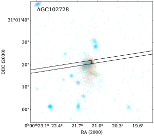
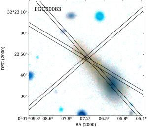
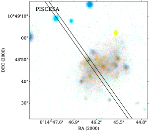
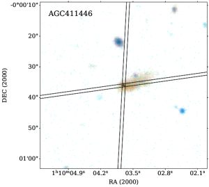
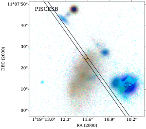
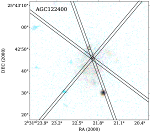
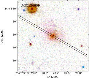
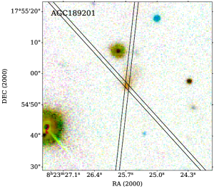
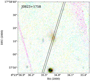
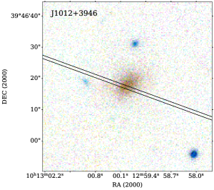
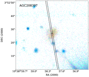
Figure 7: Finding charts of void XMP candidates from BTA program with slit positions superimposed. Inverted colours are used to underline the LSB features of dwarf morphology. North is up, East is to the left. Top row, from left to right: AGC102728 = J0000+3101, PGC00083 = J0001+3222; PISCESA = J0014+1048. Second row, from left to right: AGC411446 = J0110–0000; PISCESB = J0119+1107; AGC122400 = J0231+2542; Third row, from left to right: AGC124609=J0249+3444; KKH18=J0303+3341; AGC189201=J0823+1754, Bottom row, from left to right: J0823+1758; J1012++3946; AGC208397 = J1038+0352

Recently McQuinn et al. (2020) discussed the relation, 12+log(O/H) versus $M_{\rm B}$, for void galaxies – based on data from Pustilnik et al. (2016) and Kniazev et al. (2018) – in comparison with that for the reference sample of the late-type LV galaxies in a more typical environment (Berg et al., 2012). They used for comparison 49 void galaxies with O/H derived via the direct method. Their conclusion, based on a linear regression on the void sample data (their fig. 7, right), was that the reference and void sample relations are consistent with each other. This result implies that there is no significant difference in the average metallicity for a fixed luminosity of the void and reference sample galaxies.

We believe, however, that this issue needs a more advanced statistical analysis, which we perform below. To the naked eye, the void data in Figure 1 (black solid octagons) reveal a clear asymmetry (i.e. a downward shift) in their distribution relative to the reference sample linear regression line (solid red line). Hence, a more advanced approach should check the null hypothesis of whether the distribution of void galaxy data is consistent with the regression line describing the trend of the reference sample galaxies. This can be readily checked with the Student criterion ($t$-statistics; see, e.g., Korn & Korn, 1968); for more detail, see Bolshev & Smirnov (1983, pp.23–25, 178). If the null hypothesis is rejected at the adopted confidence level, then the visible shift of O/H for the void galaxy sample can be treated as an estimate of the difference of the two sample ’means’.

Our sample of galaxies in the Lynx–Cancer and Eridanus voids, with O/H(dir) from Pustilnik et al. (2016) and Kniazev et al. (2018), is different from that used by McQuinn et al. (2020). Namely, to the 30 galaxies from table 3 in Pustilnik et al. (2016), we add six galaxies with O/H(dir) from their table 2 and IZw18, which is also included in the Lynx–Cancer void sample. The total number of galaxies with O/H(dir) in the two voids is 55 (37+18).

We apply the Student criterion to compare two samples via their residuals relative to the linear regression line for the reference sample (Sample 1). If we subtract the linear regression value for each data point of Sample 1, we obtain a related sample Sample 1^′ of N 1 = 38 points with mean M 1^′ = 0 and standard deviation S 1^′ = 0.15 dex in log(O/H), the latter value as given in Berg et al. (2012). For the void data (Sample 2, N 2 = 55 points), for each galaxy with its absolute magnitude M_B, we compute the residual $\Delta$ log(O/H) of their real 12+log(O/H) relative to the Sample 1 regression line. These residuals comprise the Sample 2^′ with its calculated mean M 2^′ = –0.139$\pm$0.027 dex and its standard deviation S 2^′ = 0.1988 dex. If both Sample 1^′ and Sample 2^′ have asymptotically normal distribution and the same value of the mean, then the absolute value of the difference of two sample means $|$M 1^′ – M 2^′$|$ divided by the combined standard deviation estimate s_1,2, $|$M 1^′ – M 2^′$|$/s_1,2 is distributed as $t$ statistics $t(Q,N1+N2-2)$, where

$$s_{\mathrm{1},2}=\sqrt{\frac{(N1+N2)\times(N1\times(S1)^{2}+N2\times(S2)^{2})}{N1\times N2\times(N1+N2-2)}}$$ (1)

Here, $Q$ is the probability that $t$ exceeds the selected value, related to the selected probability. With the numbers in hand, we calculate that s_1,2 = 0.03848 and $|$M1^′ – M2^′ $|$/s_1,2 = 0.139/0.03848 = 3.62. Since this is larger than t(Q=0.05%,N=91) = 3.402 (Table 3.2 from Bolshev & Smirnov (1983)), this means that the $t$-criterion rejects the null hypothesis on the same ’mean’ of Samples 1^′ and 2^′ at the confidence level of $C=1-P$ = 0.999. The computed difference of the two means –0.139 dex implies that void galaxies have a mean value of gas O/H $\sim$30% lower than the reference sample. While the above confidence level of 0.999 is high, there is a caveat in the test, as the assumption of normal distribution of log(O/H) residuals for the void galaxy sample is not justified.

Therefore, we additionally apply a non-parametrical statistical criterion “2$\times$2 contingency table” (Bolshev & Smirnov, 1983). This is often used in biology and applied studies. In Pustilnik et al. (1995) and Perepelitsyna et al. (2014) we described it in detail and used it in astronomy. The goal of the method is to check whether the two considered properties in a sample of objects are independent, or are related. In this test, we consider the reference sample galaxies and the void sample with O/H(dir) data as representatives of the common population.

The first property comprises $Y$ (i.e. a void galaxy) and ’without’ $Y$ (i.e. a LV reference sample object). The second property comprises $Z$, which has the a log(O/H) residual $>$ –0.15 dex (conditionally, ’normal’ O/H), and ’without’ $Z$, which has this parameter $<$ –0.15 dex (conditionally ’low’ O/H; i.e. a stronger outlier towards a smaller O/H). Then, to test the null hypothesis that the two properties in the sample are independent of each other, we must compose a 2$\times$2 table with the general format as in Table 4 (see the first panel).

Table 4: General format of a 2$\times$2 contingency table (first panel) and its version for checking void galaxy O/H deficiency (second panel)

Property $Y$ without $Y$ Sum void non-void $Z$ $m$ $n-m$ $n$ ’normal’ O/H 34 34 68 without $Z$ $M-m$ $N-n-(M-m)$ $N-n$ ’low’ O/H 21 4 25 Sum $M$ $N-M$ $N$ 55 38 93

Here, $m$, $n-m$, $M-m$, and $N-n-(M-m)$ are the numbers of galaxies in the sample having the property combinations ($Y$, $Z$), (without $Y$, $Z$), ($Y$, without $Z$) and (without $Y$, without $Z$), respectively. As shown in Bolshev & Smirnov (1983, pp. 77–78), if the properties $Y$ and $Z$ are independent of each other, the probability of obtaining the contingency table with such numbers is described by a hypergeometric distribution. At $N>$ 25, this can be well approximated by the so-called incomplete beta function $I_{x}(a,b)$, where the parameters $x$, $a$, and $b$ can be expressed in terms of the numbers in the 2$\times$2 contingency table by the formulas (27)–(30) in Bolshev & Smirnov (1983, p. 74). See also these formulas in the appendix of Pustilnik et al. (1995).

If there is no correlation between the properties $Y$ and $Z$, the occupation numbers in the contingency table should correspond to a low probability of rejecting the Null hypothesis. For our choice, we have the following numbers (see Table 4).

The probability of the 2$\times$2 table, with the occupation numbers 34, 34, 21 and 4, calculated with the appropriate formulas for the incomplete beta function, corresponds to the confidence level of rejecting the null hypothesis of $C=0.9979$. This implies that there is a statistical relation for our sample of galaxies between the property to reside in voids and the property to have a reduced metallicity relative to the reference sample objects with the same blue luminosity. Selecting the border between the ’normal’ and ’low’ O/H as a residual log(O/H) $>$ –0.22 dex, we obtain a 2$\times$2 table with the occupation numbers 42, 38, 13 and 0. Its respective confidence level is $C=0.99967$.

As PEPK20 and McQuinn et al. (2020) recently discussed, there can be various reasons for such a reduced metallicity. To elucidate the nature of this phenomenon, one needs detailed studies of a substantially large sample of such objects. However, independent of the results of such a study, there is clear evidence that this phenomenon is related to the residence in voids.

We illustrate in Fig. 1 the significance of the difference discussed above between the two samples. The reference relation for LV galaxies from Berg et al. (2012) is shown by a red solid line. The similar linear regression on 55 galaxies from the two mentioned voids with O/H(dir) is shown by a black solid line. We also show as green empty octagons the NVG galaxies from PKPE20 and from this work, which have reliable O/H estimates O/H(s,c) via the strong-lines method of Izotov et al. (2019b) (see discussion in Appendix A.1).

We recall that these NVG objects represent the pre-selected 60 dwarf galaxies, which are candidate XMP galaxies from the ’complete’ subsample of 380 dwarfs with M${}_{\rm B}>$ –14.3 in the NVG sample (PEPK20). Therefore, we do not compare this group with the reference sample. Their discovery just supports our earlier finding that among the lowest luminosity void dwarfs there exists a substantial fraction of gas-rich objects with highly reduced metallicity. While the amount of data on void galaxy metallicities has increased substantially, a discussion of the detailed distribution and possible connection with other parameters still awaits a larger data set.

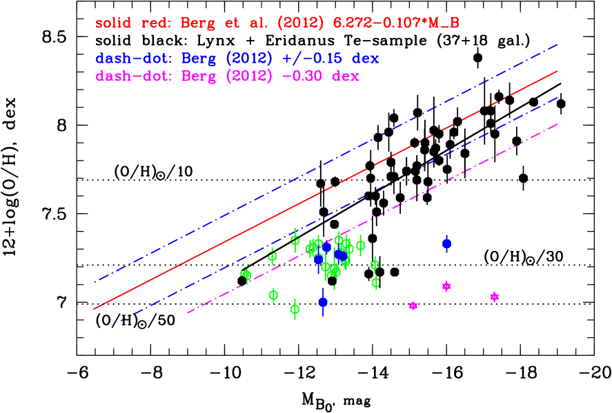
Figure 1: Positions of all galaxies with known direct O/H (black filled octagons), in Lynx–Cancer (37 objects, Pustilnik et al. (2016)), and Eridanus (18 objects, Kniazev et al. (2018)) voids. The solid black line shows the linear regression on all 55 void galaxies. It runs somewhat steeper than the reference relation (solid red) of Berg et al. (2012). As a result, for more luminous galaxies, the difference with the reference sample is subtle. However, for the range of M${}_{\rm B}\gtrsim-14$, the great majority of void galaxies sit well below the reference relation. Green empty octagons show void galaxies from PKPE20 and this work with O/H estimated via the ’strong-line’ method of Izotov et al. (2019b). Blue octagons are void dwarfs with O/H(dir) from the literature and ’strong-line’ O/H for several dwarfs in the Lynx–Cancer void. Three distant record-low XMP BCGs J0811+4730, J1234+3901 and J2229+2725 from papers by Izotov et al. (2018a, 2019, 2021) are shown as purple stars for comparison. See discussion in Sec. 4.4.

4.5 Relation of void XMP dwarfs to very young galaxies

One of the goals of this project is the search for new unusual void dwarfs resembling very young galaxies (VYGs) as predicted by Tweed et al. (2018). They are defined as objects that formed more than half their stellar mass during the last 1 Gyr.

Two record-low XMP galaxies, 12+log(O/H) = 6.98 and 7.02 dex, found by Izotov et al. (2018a) and Izotov et al. (2019a) show no tracers of the old stellar population. This fact is consistent with their extremely low metallicity if one suggests that both properties are related to the short time elapsed since the beginning of the main SF episode.

We arrived at a similar conclusion on the probable existence of young dwarfs in voids in our work devoted to the study the galaxy population of the Lynx–Cancer void (Perepelitsyna et al., 2014; Pustilnik et al., 2016). Probably it is not by chance that one of the most studied void XMP dwarfs assigned to the VYG type and the first prototype XMP dwarf is a blue compact galaxy IZw18=MRK 116 (Papaderos & Östlin, 2012). Such actively star-forming blue and UV-excess objects have attracted attention in the course of pioneering surveys of the sky. However, such outstanding star-forming (candidate) VYGs are very rare. This follows from only a few findings of XMP objects from over the whole emission-line galaxy sample in the SDSS DR14 (Izotov et al., 2019b).

From the results of our search programme, we find that in the volume limited by the nearby voids (described in PTM19), the majority of the XMP dwarfs resembling the predicted VYGs are mostly blue LSB galaxies with a much lower SF efficiency than that in actively star-forming galaxies. Therefore, in the context of the search for VYGs, obtaining their census in the local Universe and comparison with model simulations, our project looks perspective and deserves further development. While the least-massive dwarfs in voids still need more detailed predictions of their properties in model simulations, some general conclusions on the later formation of void galaxies are presented in Peper & Roukema (2021).

5 Conclusions

The NVG sample provides us with a new opportunity to search for the unusual XMP gas-rich dwarfs in voids. We performed the selection with the use of publicly available galaxy properties, based on their similarity to the properties of the known small group of XMP dwarfs. As a result, we formed a list of 60 void XMP candidates with the $M_{\rm B}$ range of [–10,–14.3] for their follow-up careful study. For 26 of them, we conducted spectroscopy with SALT, which resulted in the discovery of five new XMP dwarfs with 12+log(O/H) $\lesssim$ 7.21 dex. Here we present five more new XMP void dwarfs observed at the BTA and one XMP (J0110–0000) discovered at the BTA but first published in the paper on the SALT results. That is, to date we have discovered 10 new void XMP dwarfs. In addition, at both telescopes, we found 13 very metal-poor void dwarfs with 7.24 dex $\lesssim$ 12+log(O/H) $\lesssim$ 7.33 dex.

Summarizing the presented results and the related discussion, we draw the following conclusions.

1. In the framework of the ongoing project to search for new unusual void dwarfs among the pre-selected 60 XMP candidates residing in nearby voids, using the BTA we perform long-slit spectroscopy of 20 candidates in addition to 26 galaxies already observed at SALT. Two of these 20 objects are common with those observed at SALT.

2. For 16 of 20 galaxies observed at the BTA, we derive estimates of their gas O/H. Only two of them have a ’normal’ 12+log(O/H) for their luminosity, both of 7.89 dex. The remaining 14 of our void galaxies, with 12+log(O/H) $\leq$ 7.33 dex, appear very metal-poor. Six of them, with 12+log(O/H) = 7.00 – 7.23 dex, fall into the category of XMP galaxies, defined here as objects with Z${}_{\rm gas}\lesssim$ Z_⊙/30. Of them, J0110–0000, already presented in our previous paper PKPE20, was initially found using the BTA.

3. The O/H values of void XMP dwarfs are reduced by a factor of 2.5–4 relative to the expected values for similar galaxies in the LV reference sample of Berg et al. (2012). Their colours show a significant scatter. However, for half of them, we find blue colours of outer parts and extremely large gas-mass fraction (0.97–0.99). These properties are similar to those of the prototype XMP group, including those from the Lynx–Cancer void. This finding extends the group of the nearby candidates for VYGs to a dozen and allows us to better study their statistical properties, including their similarity and diversity.

4. The remaining eight new void dwarfs, with measured values of O/H, fall in the adjacent range of 12+log(O/H) = 7.24–7.33 dex. Such low metallicity dwarfs are still very rare, especially in the LV and the adjacent space. The division to XMP objects as those with Z $\lesssim$ Z_⊙/30 is conditional. It will not be surprising if similar objects will be identified in the group of a slightly less metal-poor galaxies. More detailed studies of this group will give insights into their evolutionary state and the possible relation to the most extreme XMP representatives.

5. In Table 3, we summarize some of the known parameters of all 10 nearby void XMP dwarfs found to date at SALT and BTA. The comprehensive multiwavelength study of the XMP void dwarfs already found will advance our understanding of galaxy formation and evolution and the specifics of star formation in such atypical conditions. This will also provide chances to confirm the discovery of the predicted rare VYGs.

Data Availability

The data underlying this article are available in Appendices B and C. Appendix C is available only in the online version of the paper.

Appendix A Check of the strong-line and the semi-empirical methods of Izotov et al. (2019, 2007)

A.1 The strong-lines method

To compare O/H derived via the strong-lines method of Izotov et al. (2019b), we selected only data where the good S/N lines [Oiii]$\lambda$4363 and [Oii]$\lambda$3727 were both available in the spectra.

In particular, we selected 15 of 66 regions in table A.2 of Izotov et al. (2019b), based purely on the SDSS DR14 spectra, as satisfying our criteria. We added 71 data points for 43 regions from the literature and this work, which include the great majority of published direct O/H estimates with 12+log(O/H) $\lesssim$ 7.5 dex and the accuracy of $\sigma$ log(O/H) $\lesssim$0.08–0.09 dex. They include, among others, three record-low metallicity XMP objects from Izotov et al. (2018a, 2019a, 2021), and four regions in DDO68 from Pustilnik et al. (2005, 2008); Izotov & Thuan (2007); Izotov, Thuan, Guseva (2012); Berg et al. (2012); Annibali et al. (2019); Little Cub (Hsyu et al., 2017), Leo P (Skillman et al., 2013), J0926+3343 (Pustilnik et al., 2010) and AGC198691 (Hirschauer et al., 2016). Data for two regions of IZw18 are adopted from Izotov & Thuan (1998), for several regions in both SBS0335–052W and SBS0335–052E from Thuan & Izotov (2005); Papaderos et al. (2006) and Izotov et al. (2009), for UGC772 from Izotov et al. (2006b); Izotov, Thuan, Guseva (2012) and Izotov & Thuan (2007), and for two regions in UGCA292 from van Zee (2000). For other objects with 12+log(O/H) $\lesssim$ 7.5 dex, the data are retrieved from Izotov et al. (2006a); Izotov, Thuan, Guseva (2012); Izotov et al. (2016, 2020), Pustilnik et al. (2003, 2006) and Guseva et al. (2009).

In Figure 2 we plot the differences of log(O/H)(s) – log(O/H)(dir) versus 12+log(O/H)(dir) for 86 points (different observations) of 55 different Hii regions in 37 galaxies with 12+log(O/H) $<$ 7.5 dex. In several popular XMP galaxies such as IZw18, SBS0335–052E, SBS0335–052W and DDO68, O/H values in their Hii regions were obtained on several independent observations.

The slope of the linear regression does not differ from zero within uncertainties. Because there is no trend of log(O/H)(s) – log(O/H)(dir) with 12+log(O/H)(dir) in the considered range of O/H, we estimate the mean value of log(O/H)(s) – log(O/H)(dir) on the whole sample. The horizontal dash-dotted line shows the weighted mean (+0.011$\pm$0.0044 dex) with the weighted rms of 0.041 dex on all 86 points. This difference is a little smaller than the similar value of +0.04 dex from paper of Izotov et al. (2019b). Due to larger statistics and the use of the weighted mean, our value of the offset of 12+log(O/H)(s) relative to 12+log(O/H)(dir) should be more reliable. Therefore, in statistical studies, where both types of O/H are used, O/H (s) and O/H (dir), in order to minimize possible bias, we suggest the use of the parameter 12+log(O/H)(s,c) = 12+log(O/H)(s) – 0.011 dex.

It is worth of mentioning that the great majority of our studied void dwarf galaxies have spectra with low excitation. Therefore, to apply the suggested correction to our new XMP void dwarfs, it is useful to check the absence of possible bias among the control sample of XMP galaxies with known O/H(dir) and those with ’low’ log(O₃₂). Accounting for the whole range of log(O₃₂) of [–0.3,+1.7] for the used 86 points, we choose the lower 1/3 of the range, that is –0.3 $<$ log(O₃₂) $<$ 0.35 (or O₃₂ $<$ 2.24). All our new XMP void galaxies have that low O₃₂. The respective 19 points with log(O₃₂) $<$ 0.35 of the whole 86 points are shown by blue symbols in Fig. 2. Their weighted mean of –0.002$\pm$0.010 dex does not differ within its uncertainty from the general weighted mean of +0.011 dex. Therefore, for our low-O₃₂ new void XMP galaxies, we use the parameter 12+log(O/H)(s,c) defined above.

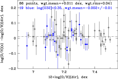
Figure 2: Relation between the difference of log(O/H)(s) (strong-lines) and log(O/H)(dir) versus 12+log(O/H)(dir) for 86 points in the range of 6.98–7.5 dex (open lozenges) with their error bars. The horizontal dash-dotted line shows the weighted mean value of 0.011 dex on all 86 points with log(O₃₂) in the range [–0.3,+1.7]. 19 of them (blue), with log(O₃₂) of –0.3 to +0.35 (with the weighted mean of –0.002$\pm$0.01). See text for references on O/H data and further discussion.

A.2 The semi-empirical method

As mentioned in Section 3, the values of T_e calculated via the direct method (i.e. with the use of auroral line [Oiii]$\lambda$4363) and those calculated with R₂₃ within the se method (Izotov & Thuan, 2007) can differ by thousands of K and this might lead to a bias in the values of O/H derived via the se method relative to those of the direct method.

The difference in estimates of T_e can be related to the large range of the ionization parameter $U$. For a given value of R₂₃, $U$ can vary by two to three orders of magnitude for Hii regions in various galaxies but this is not accounted for in the se method.

Another factor affecting the scatter of the estimate of T_e via R₂₃ can be the range of the effective temperatures T_eff of the central ionizing star (or cluster) or the related parameter (i.e. the hardness of ionizing flux).

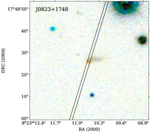
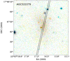
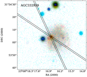
Figure 9: Finding charts of the three not-NVG sample galaxies observed at BTA, with slit positions superimposed. Inverted colours are used to underline the LSB features. North is up, East is to the left. From left to right: J0823+1748 – a distant SF galaxy in the field of AGC189201; AGC322279=J2203+1747 – non-void galaxy; AGC332939 = J2308+3154 – non-void galaxy.

However, as demonstrated by Skillman (1989, see his fig. 9) with models of Hii regions (the range of $U$ = 0.0001–0.1 and the central star T_eff of 38000, 45000 and 55000 K), the most important factor determining the ionized gas temperature T_e is $U$. In his grid, the variation of $U$ results in the largest variations of T_e for T_eff=55000 (from $\sim$8000 K for 12+log(O/H) = 7.22 dex to $\sim$4000 K at 12+log(O/H) = 7.92 dex).

For the central star with T_eff=38000 K, the range of T_e variations is smaller: from $\sim$4500 K at 12+log(O/H) = 7.22 dex to $\sim$2500 K at 12+log(O/H) = 7.92 dex. At the same time, at the fixed value of $U$, the dependence of T_e on T_eff (between 38000 and 55000 K) is small for the lowest $U$ = 0.0001 (with the range of the variance of 1000 – 1500 K) and substantially larger for the highest values of $U$ = 0.1 (range of the variance of $\sim$3000 K).

The check of the effect of hardness to the empirical estimate of T_e from observational data is outside the scope of this work. However, we can try to follow the possible effect of $U$ on T_e based on the large amount of data available in the literature. To do this at a first approximation, we draw the relation between the difference $\delta$t_e(dir,R₂₃) of the two $t_{\rm e}$ estimates (hereafter $t_{\rm e}$=T_e/10000): $t_{\rm e}$(dir) and of $t_{\rm e}$(R₂₃) (derived with the se method of Izotov & Thuan (2007)) and log(O₃₂). Parameter O₃₂ is defined as the flux ratio of the lines [Oiii]$\lambda$5007 and [Oii]$\lambda$3727. O₃₂ is an observational proxy of $U$ (e.g., Skillman (1989, fig. 7); McGaugh (1991).

In Figure 3 we show a set of $\delta$ t_e(dir,R₂₃) for 174 different measurements (135 Hii regions in 116 galaxies) versus their parameter log(O₃₂). Their gas 12+log(O/H) and parameter log(O₃₂) are distributed in wide ranges: 6.98–8.13 dex, –0.4 to +1.7, respectively. The data are collected from the papers already cited in Appendix A.1 for the lowest O/H objects – some of them include data for objects with 12+log(O/H)(dir) $>$ 7.5 dex – and from several additional papers for galaxies with 12+log(O/H)(dir) $>$ 7.5 dex. They include papers by van Zee, Haynes, Salzer (1997); van Zee & Haynes (2006); van Zee, Skillman, Haynes (2006); Bresolin et al. (2009), Pustilnik et al. (2004, 2011, 2016, 2020b), Kniazev et al. (2018) and this work.

In the top panel, we split the whole sample into three approximately equal parts on metallicity (conditionally, ’bottom’, ’middle’ and ’top’ with the borders at 12+log(O/H) = 6.98–7.5 dex, 7.5–7.82 and 7.82–8.13 dex) to probe how the relation $\delta$ t_e(dir,R₂₃) vs log(O₃₂) depends on metallicity. While the slopes of the linear regressions for the three subgroups show some variance (from $\sim$0.36 to $\sim$0.51), the rms scatter of $\delta$ t for the two higher O/H groups is reasonably small: 0.10–0.103 K. For the subgroup with the lowest metallicities, the rms scatter $\delta$ t remainss large, $\sim$0.25 K.

The above ’small’ rms$\sim$0.1 K implies that for Hii regions with 12+log(O/H) in the range of 7.5–8.1 dex, taking into account a term proportional to log(O₃₂) will mainly compensate for the difference between t_e(dir) and t_e(R₂₃) for both sufficiently high and low values of O₃₂, meaning that the uncertainty of the derived t_e is similar to that of the original estimate of t_e from Izotov & Thuan (2007).

As for the Hii regions with 12+log(O/H) $\lesssim$ 7.5 dex, the currently available data on $\delta$ t${}_{\rm e}(dir,R_{\mathrm{2}3}$) show too large scatter about the respective linear regression. Therefore, the application of such a correction to t_e(R₂₃) bears a substantial additional error in t_e, and, in turn, into an estimate of O/H. Fortunately, a purely empirical formula involving both R₂₃ and O₃₂, suggested by Izotov et al. (2019b) (the so-called strong-lines method), approximates O/H of Hii regionswell in this lowest metallicity domain, adding only $\sigma\sim$ 0.04 dex into the related uncertainty of 12+log(O/H) (see Appendix A.1).

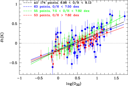
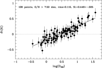
Figure 3: Relation between the difference $\delta$ t_e(dir, R₂₃) (where t=T_e/10000) and log(O₃₂) for 174 measurements of Hii regions in a range of 12+log(O/H) = 6.98–8.13 dex. Error bars show the $\pm$1$\sigma$ uncertainties of t_e(dir). Top panel: the straight lines show the linear regression fits for the whole sample (black solid) and three subsamples. The whole sample is broken into three approximately equal parts with 63, 55 and 53 points, with 12+log(O/H) in the ranges of [6.98–7.5] (blue), [7.5–7.82] (green) and [7.82–8.13] dex (red). Their rms scatter about regression lines are, respectively, 0.25, 0.099 and 0.103 K. Bottom panel: linear regression line and the scatter about it for 108 points with 12+log(O/H) $>$ 7.5 dex. Its scatter about the regression is rms=0.116 K in comparison to this parameter of 0.25 K for the remaining 63 points with 12+log(O/H) $<$ 7.5 dex.

Figure 4: A similar plot as in Figure 3 but for 63 points with 12+log(O/H) $<$ 7.5 dex. Both linear and parabolic fits are shown. See text for further explanations and discussion.

For the range of 12+log(O/H) = 7.5–8.1 dex, we adopt the linear regression in the bottom panel as:

$$\delta~{}t_{\rm e}(dir,R_{\mathrm{2}3})=+0.4463\times log(O_{\mathrm{3}2})-0.1886,(A1)$$

with the rms = 0.116 K about this line, $\sigma$(slope) = 0.026 and $\sigma$(constant) = 0.0176 K. As one can see, $\delta$t${}_{\rm e}(dir,R_{\mathrm{2}3})$ is close to zero at log(O₃₂) $\sim$ 0.46 (or O${}_{\mathrm{3}2}\sim$ 2.9). For the range of log(O₃₂) $\sim$ 0.26–0.66, $\delta$t${}_{\rm e}(dir,R_{\mathrm{2}3})$ falls within $\pm$0.1 K, which corresponds to the formal accuracy of the original se method (Izotov & Thuan, 2007). That is, the original se method can give an acceptable estimate of t_e(dir) for O${}_{\mathrm{3}2}\sim$ 1.8–4.6. For O₃₂ outside this range, the systematic error in the estimate of t_e(dir) becomes larger, reaching –0.4 K and +0.5 K at the extreme low and high values of O₃₂.

Thus, in order to use the se method of Izotov & Thuan (2007) in the whole range of the observed excitation parameter O₃₂, one should modify the original formula for $t_{\rm e}$ from Izotov & Thuan (2007):

$$t_{\rm e}=-1.3685\times\log(R_{\mathrm{2}3})+2.6258,(A2)$$

adding the term log(O₃₂) from equation (A1) as follows:

$$t_{\rm e}=-1.3685\times log(R_{\mathrm{2}3})+2.4372+0.4463\times log(O_{\mathrm{3}2})(A3)$$

As for the range of 12+log(O/H) $<$ 7.5, there is still a need for a better estimate of $t_{\rm e}$, as the strong-lines method assumes the use of corrected intensities of strong lines, which in turn depend on the adopted value of $t_{\rm e}$. In Fig. 4, we show linear and quadratic fits of $\delta$ t versus logO₃₂ for 63 points with 12+log(O/H) $<$ 7.5. As can be seen, there is a flattening in this relation for values of logO₃₂ $<$ 0.5, which the parabolic fit catches better. Indeed, although its rms scatter remains large, it certainly reduces relative to that for the linear regression (0.227 versus 0.25 K). Therefore, for the range of 12+log(O/H) $<$ 7.5, we adopt an alternative formula for $t_{\rm e}$, including the quadratic fit in Fig. 4:

$$t_{\rm e}=-1.3685\times logR_{\mathrm{2}3}+2.561-0.199\times logO_{\mathrm{3}2}+0.437\times(logO_{\mathrm{3}2})^{2}(A4)$$

The small values of $\delta$t for the lowest O/H range and logO₃₂ $<$ 0.5, imply that the se method in this range of parameters should work without the substantial systematics.

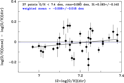
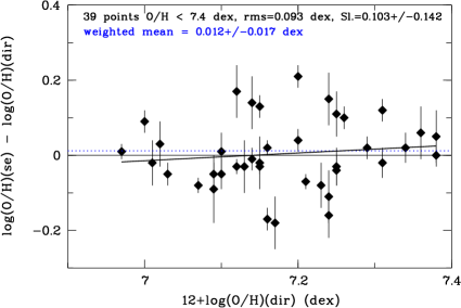
Figure 5: Top panel: relation of the difference of logO/H(mse) and logO/H(dir) versus 12+logO/H(dir) for 37 points with 12+log(O/H) $<$ 7.4 dex. The weighted mean of the difference is $\sim$ –0.008 dex with the rms scatter of $\sim$.093 dex. Bottom panel: similar relation for the difference of logO/H(se) and logO/H(dir) vs 12+logO/H(dir) for 39 points with 12+log(O/H) $<$ 7.4 dex. The weighted mean difference is $\sim$ +0.012 dex with the rms scatter of $\sim$.093 dex.

Similarly to the analysis in Izotov et al. (2019b), we limit the range of 12+log(O/H) $<$ 7.4, in order to have an opportunity to directly compare our results with theirs. In Fig. 5, we plot the difference of log(O/H)(mse) – log(O/H)(dir) and log(O/H)(se) – log(O/H)(dir), respectively, versus 12+log(O/H) on all available data. The inclined solid lines in both plots show the fitted linear regressions. In both cases, the slope does not differ significantly from zero. Therefore, we calculate the weighted means (blue dotted lines) as a measure of the mean difference of the mse and se methods relative to 12+log(O/H)(dir) in this O/H range. They are –0.008$\pm$0.010 dex for the mse method, and +0.012$\pm$0.017 dex for the se method. The rms scatter for both methods is very close, of $\sim$0.093 dex. We notice that for the se method, Izotov et al. (2019b) give the mean difference of log(O/H) $\sim$ +0.08 dex.

Despite the above conclusion of a small difference of (O/H)(se) and (O/H)(dir) in the lowest O/H range, in a wider range of O/H the difference is well traced. We illustrate this situation with the original se method in Fig. 6. Here the differences of log(O/H)(se) – log(O/H)(dir) are plotted versus 12+log(O/H)(dir). The total range of parameter logO₃₂ from $\sim$ –0.4 to $\sim$ 1.7 is divided into three ranges (–0.4,+0.2; +0.2,+0.8; and +0.8,+1.7). The points for the lower, higher and intermediate logO₃₂ ranges are shown in blue, red, and black. Now it is clearly seen that the lowest logO₃₂ points show the systematically reduced O/H relative to log(O/H)(dir), which appear smallest for the lowest 12+log(O/H) $\lesssim$ 7.3, but $\sim$ 0.2 dex lower than O/H(dir) for 12+log(O/H) $\gtrsim$ 8.0. For points with high logO₃₂, the estimates of log(O/H)(se) appear systematically elevated relative to log(O/H)(dir). For the lowest O/H, 12+log(O/H) $\lesssim$ 7.3, they show large scatter but the mean difference of $\lesssim$ 0.05 dex. For 12+log(O/H) $\sim$ 8.0 dex, the mean difference is $\sim$ +0.2 dex.

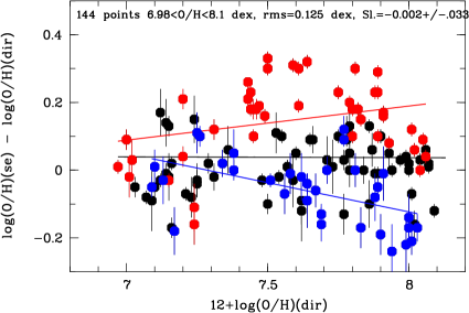
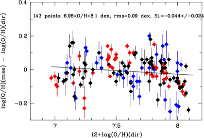
Figure 6: Top panel: relation of the difference log(O/H)(se) – log(O/H)(dir) versus 12+log(O/H)(dir) on a sample of 144 points from the literature, with 6.98 $<$ 12+log(O/H) $<$ 8.1 dex. The black line shows the linear regression fit for the whole data with the rms = 0.125 dex. Blue, black and red points show separately the data with low, middle and high O₃₂, corresponding to logO₃₂ in the ranges (–0.4, +0.2; +0.2, +0.8; and +0.8, +1.7) respectively. Blue and red solid lines show respective linear regressions for low and high O₃₂ subsamples. Bottom panel: same as in top panel, but for the mse method for 143 points. Its scatter on the linear regression is significantly smaller, rms = 0.09 dex.

The se method, based on the modified equations (A3) and (A4) for the estimate of t_e, which includes the logO₃₂ term, allows us to remove the systematics inherent to the original se method by Izotov & Thuan (2007), as illustrated in Fig. 6 (bottom panel). As can be seen, blue and red points show the even scatter on the linear regression line drawn on the whole sample. Moreover, as a result of the removal of systematics, the general scatter on the linear regression is reduced substantially: from rms = 0.125 dex in Fig. 6 (top; original se method) to rms = 0.090 dex for the mse method. This indicates that the addition of a term with logO₃₂ to the original formula for T_e from Izotov & Thuan (2007) indeed improves the accuracy of O/H for the indicated O/H range for a wide range of O₃₂.

For the practical use of the mse method, it is necessary to fit a relation of 12+log(O/H)(dir) versus 12+log(O/H)(mse) (Y versus X in the equation below) as follows:

$$Y=0.960(\pm 0.024)~{}X+0.318(\pm 0.184)~{}~{}~{}~{}(A5)$$

The rms scatter of 143 analysed points on the linear regression is 0.090 dex. Over the range of 12+log(O/H)(mse) = 7.0–8.1 dex, the related correction, that is log(O/H)(dir) – log(O/H)(mse), varies between +0.038 dex and –0.006 dex, respectively. We call the parameter $Y$, calculated in equation (A5), a corrected log(O/H)(mse,c) and apply it in further O/H estimates as a well approximating log(O/H)(dir) without an additional offset. The intrinsic accuracy of log(O/H)(mse,c) is 0.09 dex.

The residual scatter between 12+log(O/H)(mse) and 12+log(O/H)(dir) can be attributed partly to the accuracy of the original O/H(dir), and partly to the unaccounted factor of the ionizing radiation hardness. It is clear from the models (e.g., Skillman, 1989) that its effect on T_e can be comparable, in principle, with the effect of the ionization parameter $U$ (or of its proxy O₃₂). However, there are very few data on the radiation hardness in various Hii regions. Because of various selection effects inherent to samples with the sufficiently strong line [Oiii]$\lambda$4363, used for O/H(dir), their hardness parameter falls into a range that is not wide. The above scatter could also arise from differences in the method used to estimate the extinction coefficient CH$\beta$ (affecting O₃₂) and the value of EW(abs) (affecting R₂₃) that were used in our analysis of spectra from the literature.

For the majority of our void galaxy spectra, the value of logO₃₂ falls below 0.5. Therefore, one expects some corrections of t_e calculated in papers by Pustilnik et al. (2016, 2020b) and Kniazev et al. (2018) with the original se method, with a related small correction of $\Delta$ log(O/H). We employ this mse method and present in Tables B1–B7 the O/H estimates derived with this method, O/H(mse,c), for comparison derived with other methods.

Appendix B Tables with line fluxes and derived parameters

The tables in this appendix include the measured line fluxes F($\lambda$) (relative to the flux of H$\beta$) and the line intensities I($\lambda$), corrected for extinction and the underlying stellar Balmer absorption, with their errors.

The tables also include the measured EWs of the H$\beta$ emission line and the derived parameters: the extinction coefficient C (H$\beta$), the equivalent width of the underlying stellar Balmer absorptions EW(abs), the electron temperatures T_e(Oiii) – estimated with the mse method (see Appendix A2) – if it was not possible with the direct method, and T_e(Oii), the two temeperatures, corresponding to two qzones of oxygen ionization. We also present the derived oxygen abundances in two stages of ionization and the total value of O/H, including its value in units of 12+log(O/H) as derived either via the direct method, or the mse method, when [Oiii]$\lambda$4363 was not detected.

For the range of 12+log(O/H) $<$ 7.5 dex, we also present O/H(s,c) and O/H(se,c) as described in Appendices A1 and A2. The flux in the emission line H$\beta$ is in units of 10^-16 erg s^-1cm^-2. Its error reflects the measurement uncertainty only and does not include probable loss on the slit. Electron densities n_e in Hii regions could not be estimated when the doublet [Sii]$\lambda\lambda$6716,6731 was outside the observed wavelength range. In this case, we adopted n_e to be 10 per cm³, typical of Hii regions in dIrr galaxies.

Table 5: Measured and corrected line intensities, and derived oxygen abundances

	PGC000083a=J0001+3222a		PGC000083b=J0001+3222b		PiscesA=J0014+1048
$\lambda_{0}$(Å) Ion	F($\lambda$)/F(H$\beta$)	I($\lambda$)/I(H$\beta$)	F($\lambda$)/F(H$\beta$)	I($\lambda$)/I(H$\beta$)	F($\lambda$)/F(H$\beta$)	I($\lambda$)/I(H$\beta$)
3727 [O ii]	1.768$\pm$0.138	1.530$\pm$0.144	0.612$\pm$0.105	0.664$\pm$0.120	1.196$\pm$0.098	1.182$\pm$0.108
4101 H$\delta$	—	—	0.190$\pm$0.028	0.287$\pm$0.056	0.161$\pm$0.019	0.297$\pm$0.044
4340 H$\gamma$	0.352$\pm$0.023	0.475$\pm$0.042	0.402$\pm$0.028	0.475$\pm$0.042	0.359$\pm$0.025	0.457$\pm$0.039
4861 H$\beta$	1.000$\pm$0.049	1.000$\pm$0.061	1.000$\pm$0.049	1.000$\pm$0.053	1.000$\pm$0.040	1.000$\pm$0.045
4959 [O iii]	0.264$\pm$0.020	0.222$\pm$0.020	0.498$\pm$0.027	0.474$\pm$0.027	0.551$\pm$0.021	0.497$\pm$0.021
5007 [O iii]	0.880$\pm$0.035	0.741$\pm$0.035	1.360$\pm$0.056	1.287$\pm$0.056	1.689$\pm$0.059	1.519$\pm$0.058
6563 H$\alpha$	3.196$\pm$0.118	2.725$\pm$0.130	—	—	3.264$\pm$0.103	2.752$\pm$0.104
6717 [S ii]	0.281$\pm$0.022	0.230$\pm$0.022	—	—	—	—
6731 [S ii]	0.179$\pm$0.020	0.147$\pm$0.020	—	—	—	—
C(H$\beta$) dex	0.04$\pm$0.05		0.17$\pm$0.06		0.12$\pm$0.04
EW(abs) Å	3.10$\pm$0.27		2.30$\pm$0.76		3.85$\pm$0.37
F(H$\beta$)	1.68$\pm$0.06		1.40$\pm$0.04		7.76$\pm$0.21
EW(H$\beta$) Å	17$\pm$ 1		54$\pm$ 2		38$\pm$ 1
$T_{\rm e}$(OIII)(K)	21033$\pm$1107		20128$\pm$1116		18478$\pm$1059
$T_{\rm e}$(OII)(K)	15971$\pm$284		15619$\pm$67		14934$\pm$89
$N_{\rm e}$(SII)(cm-3)	10$\pm$10		10$\pm$10		10$\pm$10
O+/H+($\times$105)	1.148$\pm$0.124		0.532$\pm$0.096		1.086$\pm$0.101
O++/H+($\times$105)	0.373$\pm$0.042		0.745$\pm$0.088		1.021$\pm$0.131
O/H($\times$105)	1.521$\pm$0.131		1.277$\pm$0.131		2.107$\pm$0.165
12+log(O/H)(mse,c)	7.19$\pm$0.10		7.12$\pm$0.10		7.33$\pm$0.10
12+log(O/H)(se,c)	7.25$\pm$0.10		7.05$\pm$0.10		7.29$\pm$0.10
12+log(O/H)(s,c)	7.17$\pm$0.05		7.13$\pm$0.05		7.26$\pm$0.05

Table 6: Measured and corrected line intensities, and derived oxygen abundances

	AGC411446=J0110–00000		PiscesB=J0119+1107		AGC122400=J0231+3542
$\lambda_{0}$(Å) Ion	F($\lambda$)/F(H$\beta$)	I($\lambda$)/I(H$\beta$)	F($\lambda$)/F(H$\beta$)	I($\lambda$)/I(H$\beta$)	F($\lambda$)/F(H$\beta$)	I($\lambda$)/I(H$\beta$)
3727 [O ii]	0.918$\pm$0.108	0.776$\pm$0.109	2.551$\pm$0.149	2.327$\pm$0.169	1.600$\pm$0.750	1.192$\pm$0.664
4340 H$\gamma$	0.227$\pm$0.024	0.386$\pm$0.058	0.300$\pm$0.062	0.446$\pm$0.143	0.114$\pm$0.059	0.448$\pm$0.464
4861 H$\beta$	1.000$\pm$0.044	1.000$\pm$0.055	1.000$\pm$0.055	1.000$\pm$0.091	1.000$\pm$0.202	1.000$\pm$0.340
4959 [O iii]	0.282$\pm$0.033	0.239$\pm$0.033	0.300$\pm$0.025	0.258$\pm$0.025	0.543$\pm$0.138	0.361$\pm$0.137
5007 [O iii]	0.848$\pm$0.044	0.717$\pm$0.044	1.006$\pm$0.051	0.862$\pm$0.051	1.657$\pm$0.263	1.097$\pm$0.261
6548 [N ii]	0.033$\pm$0.065	0.028$\pm$0.065	—	—	—	—
6563 H$\alpha$	3.111$\pm$0.141	2.711$\pm$0.158	—	—	—	—
6584 [N ii]	0.102$\pm$0.079	0.086$\pm$0.079	—	—	—	—
6717 [S ii]	0.171$\pm$0.087	0.144$\pm$0.087	—	—	—	—
6731 [S ii]	0.080$\pm$0.078	0.068$\pm$0.078	—	—	—	—
C(H$\beta$) dex	0.00$\pm$0.06		0.08$\pm$0.04		0.15$\pm$0.04
EW(abs) Å	3.65$\pm$0.34		2.50$\pm$1.00		4.50$\pm$1.25
F(H$\beta$)a	1.09$\pm$0.03		7.19$\pm$0.27		0.48$\pm$0.04
EW(H$\beta$) Å	20$\pm$ 1		16$\pm$ 1		9$\pm$ 1
$T_{\rm e}$(OIII)(K)	22319$\pm$1187		19673$\pm$1086		19793$\pm$2972
$T_{\rm e}$(OII)(K)	16271$\pm$248		14947$\pm$67		14938$\pm$228
$N_{\rm e}$(SII)(cm-3)	10$\pm$10		10$\pm$10		10$\pm$10
O+/H+($\times$105)	0.551$\pm$0.081		2.133$\pm$0.158		1.094$\pm$0.781
O++/H+($\times$105)	0.329$\pm$0.038		0.496$\pm$0.062		0.638$\pm$0.236
O/H($\times$105)	0.880$\pm$0.090		2.629$\pm$0.170		1.732$\pm$0.816
12+log(O/H)(mse,c)	6.96$\pm$0.10		7.43$\pm$0.10		7.25$\pm$0.20
12+log(O/H)(se,c)	6.95$\pm$0.10		7.42$\pm$0.10		7.18$\pm$0.20
12+log(O/H)(s,c)	7.00$\pm$0.05		7.31$\pm$0.05		7.19$\pm$0.12

Table 7: Measured and corrected line intensities, and derived oxygen abundances

	J0823+1758		AGC239144=J1349+3544		AGC249590=J1440+3416
$\lambda_{0}$(Å) Ion	F($\lambda$)/F(H$\beta$)	I($\lambda$)/I(H$\beta$)	F($\lambda$)/F(H$\beta$)	I($\lambda$)/I(H$\beta$)	F($\lambda$)/F(H$\beta$)	I($\lambda$)/I(H$\beta$)
3727 [O ii]	1.807$\pm$0.149	1.908$\pm$0.173	2.575$\pm$0.384	2.180$\pm$0.397	1.471$\pm$0.136	1.478$\pm$0.150
4101 H$\delta$	—	—	—	—	0.143$\pm$0.020	0.245$\pm$0.043
4340 H$\gamma$	0.381$\pm$0.025	0.478$\pm$0.041	0.181$\pm$0.038	0.332$\pm$0.099	0.397$\pm$0.027	0.481$\pm$0.039
4861 H$\beta$	1.000$\pm$0.039	1.000$\pm$0.045	1.000$\pm$0.066	1.000$\pm$0.082	1.000$\pm$0.036	1.000$\pm$0.040
4959 [O iii]	0.454$\pm$0.027	0.415$\pm$0.026	0.323$\pm$0.044	0.273$\pm$0.044	0.357$\pm$0.021	0.328$\pm$0.021
5007 [O iii]	1.514$\pm$0.053	1.376$\pm$0.053	0.857$\pm$0.062	0.726$\pm$0.062	1.178$\pm$0.038	1.077$\pm$0.038
6548 [N ii]	—	—	0.084$\pm$0.205	0.071$\pm$0.205	—	—
6563 H$\alpha$	3.387$\pm$0.103	2.760$\pm$0.100	3.177$\pm$0.295	2.787$\pm$0.332	3.201$\pm$0.110	2.741$\pm$0.111
6584 [N ii]	—	—	0.253$\pm$0.217	0.214$\pm$0.217	—	—
C(H$\beta$) dex	0.19$\pm$0.04		0.00$\pm$0.12		0.12$\pm$0.04
EW(abs) Å	2.00$\pm$0.39		2.00$\pm$0.28		2.80$\pm$0.34
F(H$\beta$)a	2.40$\pm$0.10		0.34$\pm$0.02		0.46$\pm$0.01
EW(H$\beta$) Å	24$\pm$ 1		11$\pm$ 1		33$\pm$ 1
$T_{\rm e}$(OIII)(K)	18066$\pm$1079		15179$\pm$1374		19536$\pm$1089
$T_{\rm e}$(OII)(K)	14889$\pm$145		13994$\pm$668		14954$\pm$49
$N_{\rm e}$(SII)(cm-3)	10$\pm$10		10$\pm$10		10$\pm$10
O+/H+($\times$105)	1.770$\pm$0.169		2.464$\pm$0.590		1.352$\pm$0.138
O++/H+($\times$105)	0.953$\pm$0.129		0.799$\pm$0.191		0.632$\pm$0.076
O/H($\times$105)	2.722$\pm$0.213		3.263$\pm$0.620		1.984$\pm$0.158
12+log(O/H)(mse,c)	7.44$\pm$0.10		7.39$\pm$0.13		7.31$\pm$0.10
12+log(O/H)(se,c)	7.42$\pm$0.10		7.37$\pm$0.12		7.28$\pm$0.10
12+log(O/H)(s,c)	7.33$\pm$0.05		7.25$\pm$0.07		7.23$\pm$0.05

Table 8: Measured and corrected line intensities, and derived oxygen abundances

	J1444+4242a		J1444+4242b		PGC2081790=J1447+3630
$\lambda_{0}$(Å) Ion	F($\lambda$)/F(H$\beta$)	I($\lambda$)/I(H$\beta$)	F($\lambda$)/F(H$\beta$)	I($\lambda$)/I(H$\beta$)	F($\lambda$)/F(H$\beta$)	I($\lambda$)/I(H$\beta$)
3727 [O ii]	1.162$\pm$0.088	1.070$\pm$0.092	1.233$\pm$0.115	1.161$\pm$0.120	1.868$\pm$0.061	1.709$\pm$0.063
3967 [Ne iii] + H7	—	—	—	—	0.109$\pm$0.017	0.226$\pm$0.046
4101 H$\delta$	0.132$\pm$0.017	0.273$\pm$0.048	0.110$\pm$0.016	0.212$\pm$0.043	0.195$\pm$0.018	0.299$\pm$0.034
4340 H$\gamma$	0.317$\pm$0.025	0.441$\pm$0.045	0.416$\pm$0.024	0.477$\pm$0.035	0.338$\pm$0.018	0.428$\pm$0.029
4861 H$\beta$	1.000$\pm$0.032	1.000$\pm$0.038	1.000$\pm$0.035	1.000$\pm$0.042	1.000$\pm$0.024	1.000$\pm$0.028
4959 [O iii]	0.471$\pm$0.024	0.419$\pm$0.024	0.278$\pm$0.026	0.253$\pm$0.026	0.530$\pm$0.013	0.485$\pm$0.013
5007 [O iii]	1.403$\pm$0.045	1.248$\pm$0.045	0.877$\pm$0.036	0.797$\pm$0.036	1.616$\pm$0.036	1.478$\pm$0.036
6563 H$\alpha$	—	—	—	—	2.865$\pm$0.057	2.756$\pm$0.066
C(H$\beta$) dex	0.04$\pm$0.04		0.04$\pm$0.05		0.00$\pm$0.03
EW(abs) Å	2.50$\pm$0.25		1.25$\pm$0.22		4.70$\pm$0.41
F(H$\beta$)a	0.77$\pm$0.02		0.56$\pm$0.02		1.78$\pm$0.03
EW(H$\beta$) Å	21$\pm$0.4		13$\pm$0.3		50$\pm$ 1
$T_{\rm e}$(OIII)(K)	19443$\pm$1060		21189$\pm$1113		17909$\pm$1016
$T_{\rm e}$(OII)(K)	14958$\pm$36		16011$\pm$279		14867$\pm$156
$N_{\rm e}$(SII)(cm-3)	10$\pm$10		10$\pm$10		10$\pm$10
O+/H+($\times$105)	0.978$\pm$0.085		0.864$\pm$0.100		1.592$\pm$0.078
O++/H+($\times$105)	0.757$\pm$0.090		0.400$\pm$0.045		1.065$\pm$0.135
O/H($\times$105)	1.736$\pm$0.123		1.265$\pm$0.109		2.657$\pm$0.156
12+log(O/H)(mse,c)	7.25$\pm$0.10		7.12$\pm$0.10		7.43$\pm$0.10
12+log(O/H)(se,c)	7.18$\pm$0.10		7.08$\pm$0.10		7.40$\pm$0.11
12+log(O/H)(s,c)	7.20$\pm$0.05		7.11$\pm$0.05		7.32$\pm$0.04

Table 9: Measured and corrected line intensities, and derived oxygen abundances

	J1522+4201		J2103–0049		AGC321307=J2214+2540
$\lambda_{0}$(Å) Ion	F($\lambda$)/F(H$\beta$)	I($\lambda$)/I(H$\beta$)	F($\lambda$)/F(H$\beta$)	I($\lambda$)/I(H$\beta$)	F($\lambda$)/F(H$\beta$)	I($\lambda$)/I(H$\beta$)
3727 [O ii]	2.481$\pm$0.169	2.191$\pm$0.171	1.621$\pm$0.084	1.594$\pm$0.085	2.764$\pm$0.384	2.729$\pm$0.396
4340 H$\gamma$	0.208$\pm$0.026	0.314$\pm$0.065	—	—	—	—
4861 H$\beta$	1.000$\pm$0.037	1.000$\pm$0.057	1.000$\pm$0.028	1.000$\pm$0.039	1.000$\pm$0.103	1.000$\pm$0.224
4959 [O iii]	0.390$\pm$0.028	0.344$\pm$0.028	0.311$\pm$0.011	0.305$\pm$0.011	0.764$\pm$0.091	0.751$\pm$0.092
5007 [O iii]	1.026$\pm$0.037	0.906$\pm$0.037	0.913$\pm$0.026	0.897$\pm$0.026	2.800$\pm$0.223	2.754$\pm$0.223
6563 H$\alpha$	3.000$\pm$0.087	2.736$\pm$0.102	2.767$\pm$0.066	2.733$\pm$0.075	2.790$\pm$0.227	2.817$\pm$0.337
C(H$\beta$) dex	0.00$\pm$0.04		0.00$\pm$0.03		0.01$\pm$0.10
EW(abs) Å	2.30$\pm$0.68		0.10$\pm$0.16		0.05$\pm$0.61
F(H$\beta$)a	0.77$\pm$0.02		0.50$\pm$0.01		0.55$\pm$0.04
EW(H$\beta$) Å	17.4$\pm$0.55		2.04$\pm$0.04		3.09$\pm$0.25
$T_{\rm e}$(OIII)(K)	19435$\pm$1080		20085$\pm$1034		13512$\pm$1212
$T_{\rm e}$(OII)(K)	14958$\pm$36		14911$\pm$116		13014$\pm$836
$N_{\rm e}$(SII)(cm-3)	10$\pm$10		10$\pm$10		10$\pm$10
O+/H+($\times$105)	2.003$\pm$0.157		1.472$\pm$0.086		3.939$\pm$1.048
O++/H+($\times$105)	0.569$\pm$0.069		0.511$\pm$0.055		3.800$\pm$0.965
O/H($\times$105)	2.572$\pm$0.172		1.983$\pm$0.103		7.739$\pm$1.424
12+log(O/H)(mse,c)	7.42$\pm$0.10		7.31$\pm$0.09		7.89$\pm$0.10
12+log(O/H)(se,c)	7.41$\pm$0.11		7.30$\pm$0.10		7.75$\pm$0.10
12+log(O/H)(s,c)	7.30$\pm$0.05		7.21$\pm$0.04		—

Table 10: Measured and corrected line intensities, and derived oxygen and neon abundances

	AGC332939=J2308+3154		AGC334513=J2348+2335
$\lambda_{0}$(Å) Ion	F($\lambda$)/F(H$\beta$)	I($\lambda$)/I(H$\beta$)	F($\lambda$)/F(H$\beta$)	I($\lambda$)/I(H$\beta$)
3727 [O ii]	0.720$\pm$0.024	0.714$\pm$0.026	1.784$\pm$0.143	1.750$\pm$0.165
4101 H$\delta$	0.190$\pm$0.011	0.200$\pm$0.015	—	—
4340 H$\gamma$	0.363$\pm$0.015	0.369$\pm$0.017	0.324$\pm$0.028	0.471$\pm$0.105
4363 [O iii]	0.076$\pm$0.010	0.076$\pm$0.010	—	—
4471 He i	0.033$\pm$0.003	0.033$\pm$0.003	—	—
4861 H$\beta$	1.000$\pm$0.031	1.000$\pm$0.032	1.000$\pm$0.038	1.000$\pm$0.078
4959 [O iii]	1.414$\pm$0.049	1.402$\pm$0.049	0.351$\pm$0.029	0.306$\pm$0.029
5007 [O iii]	3.727$\pm$0.114	3.695$\pm$0.115	1.081$\pm$0.040	0.939$\pm$0.040
6548 [N ii]	0.017$\pm$0.014	0.016$\pm$0.014	0.000$\pm$0.054	0.000$\pm$0.054
6563 H$\alpha$	2.811$\pm$0.086	2.791$\pm$0.094	3.405$\pm$0.164	2.740$\pm$0.168
6584 [N ii]	0.021$\pm$0.021	0.021$\pm$0.021	0.081$\pm$0.081	0.063$\pm$0.072
6717 [S ii]	0.093$\pm$0.018	0.093$\pm$0.018	0.243$\pm$0.028	0.188$\pm$0.025
6731 [S ii]	0.069$\pm$0.018	0.068$\pm$0.018	0.108$\pm$0.027	0.084$\pm$0.024
C(H$\beta$) dex	0.00$\pm$0.04		0.15$\pm$0.06
EW(abs) Å	0.75$\pm$0.62		2.55$\pm$1.19
F(H$\beta$)a	32.1$\pm$0.62		3.72$\pm$0.06
EW(H$\beta$) Å	89$\pm$ 2		19$\pm$ 1
$T_{\rm e}$(OIII)(K)	15172$\pm$977		19757$\pm$1102
$T_{\rm e}$(OII)(K)	13990$\pm$476		14941$\pm$80
$N_{\rm e}$(SII)(cm-3)	45$\pm$455		10$\pm$10
O+/H+($\times$105)	0.811$\pm$0.104		1.606$\pm$0.154
O++/H+($\times$105)	4.084$\pm$0.665		0.547$\pm$0.067
O/H($\times$105)	4.895$\pm$0.673		2.154$\pm$0.168
12+log(O/H)(dir)	7.69$\pm$0.06		—
12+log(O/H)(mse,c)	—		7.34$\pm$0.10
12+log(O/H)(se,c)	—		7.32$\pm$0.11
12+log(O/H)(s,c)	—		7.24$\pm$0.05

Table 11: Measured and corrected line intensities, and derived oxygen and neon abundances

	AGC124609=J0249+3444		AGC189201=J0823+1754
$\lambda_{0}$(Å) Ion	F($\lambda$)/F(H$\beta$)	I($\lambda$)/I(H$\beta$)	F($\lambda$)/F(H$\beta$)	I($\lambda$)/I(H$\beta$)
3727 [O ii]	0.733$\pm$0.031	0.720$\pm$0.032	0.760$\pm$0.046	0.880$\pm$0.056
3835 H9	0.046$\pm$0.018	0.068$\pm$0.029	—	—
3967 [Ne iii] + H7	0.266$\pm$0.008	0.284$\pm$0.011	0.178$\pm$0.009	0.251$\pm$0.015
4101 H$\delta$	0.237$\pm$0.007	0.256$\pm$0.010	0.223$\pm$0.006	0.290$\pm$0.011
4340 H$\gamma$	0.463$\pm$0.012	0.476$\pm$0.014	0.404$\pm$0.010	0.466$\pm$0.013
4363 [O iii]	0.120$\pm$0.005	0.118$\pm$0.005	0.051$\pm$0.006	0.053$\pm$0.006
4388 He i	—	—	0.009$\pm$0.003	0.009$\pm$0.003
4438 He i	—	—	0.009$\pm$0.003	0.009$\pm$0.003
4471 He i	—	—	0.023$\pm$0.006	0.023$\pm$0.006
4686 He ii	0.040$\pm$0.006	0.039$\pm$0.006	—	—
4712 [Ar iv] + He i	0.021$\pm$0.004	0.021$\pm$0.004	—	—
4861 H$\beta$	1.000$\pm$0.023	1.000$\pm$0.024	1.000$\pm$0.020	1.000$\pm$0.021
4959 [O iii]	2.034$\pm$0.046	1.998$\pm$0.046	0.630$\pm$0.012	0.603$\pm$0.012
5007 [O iii]	6.056$\pm$0.124	5.951$\pm$0.124	1.901$\pm$0.032	1.808$\pm$0.031
5869 He ii	—	—	0.127$\pm$0.006	0.109$\pm$0.005
6548 [N ii]	—	—	0.006$\pm$0.011	0.004$\pm$0.009
6563 H$\alpha$	—	—	3.424$\pm$0.055	2.756$\pm$0.049
6584 [N ii]	—	—	0.025$\pm$0.014	0.020$\pm$0.012
6678 He i	—	—	0.037$\pm$0.006	0.029$\pm$0.005
6717 [S ii]	—	—	0.096$\pm$0.003	0.076$\pm$0.003
6731 [S ii]	—	—	0.079$\pm$0.006	0.062$\pm$0.005
C(H$\beta$) dex	0.00$\pm$0.03		0.25$\pm$0.02
EW(abs) Å	1.50$\pm$0.42		3.15$\pm$0.35
F(H$\beta$)a	14.77$\pm$0.19		3.53$\pm$0.04
EW(H$\beta$) Å	89$\pm$ 1.5		101$\pm$ 1
$T_{\rm e}$(OIII)(K)	15146$\pm$341		18464$\pm$1209
$T_{\rm e}$(OII)(K)	13978$\pm$167		14933$\pm$103
$N_{\rm e}$(SII)(cm-3)	10$\pm$10		235$\pm$161
O+/H+($\times$105)	0.820$\pm$0.048		0.829$\pm$0.057
O++/H+($\times$105)	6.415$\pm$0.378		1.223$\pm$0.175
O+++/H+($\times$105)	0.542$\pm$0.154		—
O/H($\times$105)	7.778$\pm$0.374		2.052$\pm$0.184
12+log(O/H)(dir)	7.89$\pm$0.02		7.31$\pm$0.04
12+log(O/H)(se,c)	8.00$\pm$0.10		7.29$\pm$0.09
12+log(O/H)(mse,c)	7.86$\pm$0.10		7.33$\pm$0.09
12+log(O/H)(s,c)	—		7.27$\pm$0.04
Ne++/H+($\times$105)	1.032$\pm$0.074		0.235$\pm$0.041
ICF(Ne)	1.073		1.176
Ne/H($\times$105)	1.11$\pm$0.08		0.28$\pm$0.05
12+log(Ne/H)	7.04$\pm$0.03		6.44$\pm$0.08
log(Ne/O)	-0.85$\pm$0.04		-0.87$\pm$0.09

Appendix C On-line data. Finding charts with slit positions and plots of 1D spectra

In Figures S1–S2 we provide the slit positions for each of our program galaxy overlaid on the galaxy images taken either from DECaLS (Dey et al., 2019), or PanSTARRS PS1 (Flewelling et al., 2020), or SDSS (Abazajian et al., 2009; Abolfathi et al., 2018) databases. In Figure S3 we show the slit positions for three observed galaxies which are not in the XMP void candidate list.

The plots of obtained 1D spectra are presented in Figures S4–S5 of this Appendix. Here on $X$ axis the wavelengths are shown in Å. In $Y$ axis the measured flux densities are marked in units of 10^-16 erg s^-1 cm^-2 Å^-1. The names of objects are inserted along with their adopted value of 12+log(O/H), when available.

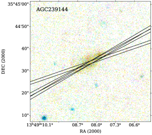
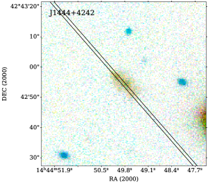
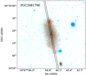
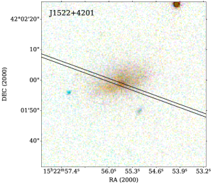
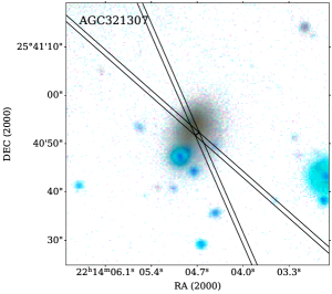
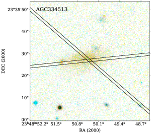
Figure 8: Finding charts of void XMP candidates from BTA program with slit positions superimposed. Inverted colours are used to underline the LSB features of dwarf morphology. North is up, East is to the left. Top row, from left to right: AGC239144=J1349+3544; AGC249590=J1440+3416; J1444+4242; Second row, from left to right: PGC2081790 = J1447+3630, J1522+4201; J2103–0049; Bottom row, from left to right: AGC321307=J2214+2540; AGC334513=J2348+2335.

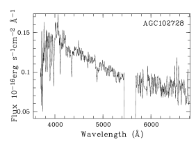
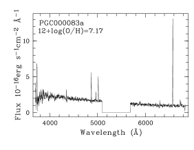
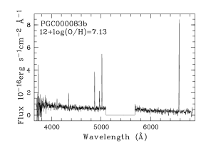
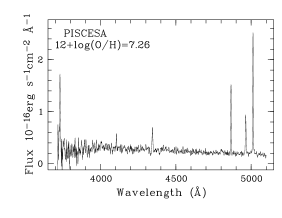
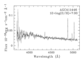
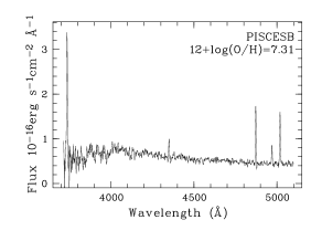
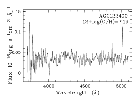
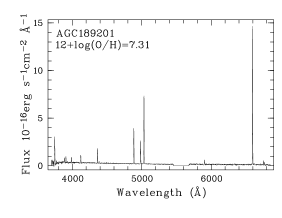
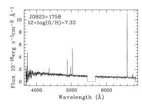
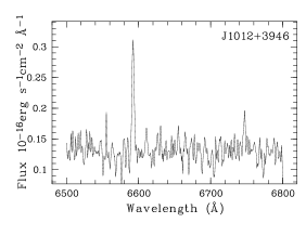
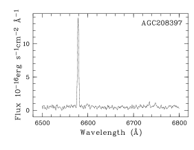
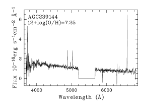
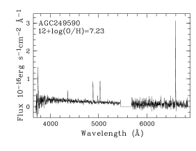
Figure 10: 1D spectra of void XMP candidates obtained with BTA. The wavelengths on the $X$ axis are observed, not in the rest-frame. The flux densities on the $Y$ axis are shown in units of 10^-16 ergs s^-1cm^-2 Å^-1. The galaxy name and derived value of 12+log(O/H) are shown at the top of each box. Top panel, from left to right: AGC102728=J0000+3101. Only very faint emission H$\alpha$ is detected besides Balmer absorptions. PGC00083=J0001+3222. Spectra of two knots are shown with somewhat different O/H = 7.17 for ”a” and 7.13 for ”b”. Second panel, from left to right: PiscesA=J0014+1048, O/H=7.26; AGC411446=J011003–000036, O/H = 7.00; PiscesB=J0119+1107, O/H = 7.31; Third panel, left to right: AGC122400 = J0231+3542, O/H = 7.19; AGC124609=J0249+3444, O/H = 7.89; KKH18=J0303+3341, red spectrum. Fourth panel, from left to right: AGC189201=J0823+1754, O/H = 7.31; J0823+1758, O/H = 7.33; J1012+3946, red spectrum. Bottom panel, from left to right: back-up time red spectrum of AGC208397 = J1038+0352; AGC239144 = J1349+3544, O/H = 7.25; AGC249590=J1440+3416, O/H = 7.23.

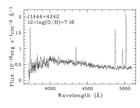
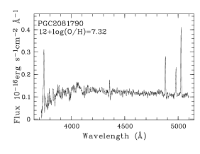
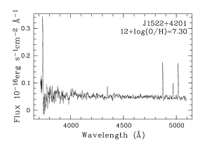
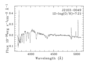
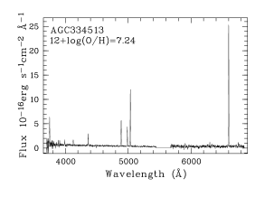
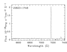
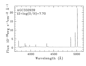
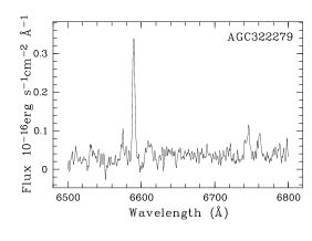
Figure 11: 1D spectra of void XMP candidates obtained with BTA. The galaxy name and derived value of 12+$\log$(O/H) are shown at the top of each box. Top panel, from left to right: J1444+4242, O/H = 7.16 (average on 2 knots); PGC2081790 = J1447+3630, O/H = 7.33; J1522+4201, O/H = 7.30; Second panel, left to right: J2103-0049, O/H = 7.21; AGC321307=J2214+2540, O/H = 7.89; AGC334513 = J2348+2335, O/H = 7.24. Bottom panel, from left to right: Non-void galaxies: red spectrum of J0823+1748 with z = 0.092, AGC332939=J2308+3154, O/H = 7.69; red spectrum of AGC322279=J2203+1747.

References

- Abazajian et al. (2009) Abazajian K. N. et al., 2009, ApJS, 182, 543
- Abolfathi et al. (2018) Abolfathi B. et al., 2018, ApJS, 335, 42
- Afanasiev & Moiseev (2005) Afanasiev V. L., Moiseev A. V., 2005, Astron.Lett., 31, 194
- Annibali et al. (2019) Annibali F. et al., 2019, MNRAS, 482, 3892
- Asplund et al. (2009) Asplund M., Grevesse N., Sauval A. J., Scott P., 2009, ARA&A, 47, 481
- Berg et al. (2012) Berg D. A. et al., 2012, ApJ, 754, 98
- Bolshev & Smirnov (1983) Bolshev L. N., Smirnov N. V., 1983, Tables of Mathematical Statistics (in Russian). Nauka, Moscow, p.415.(available at, e.g. https://en.booksee.org/book/467193)
- Bresolin et al. (2009) Bresolin F., Gieren W., Kudritzki R.-P., Pietrzynski G., Urbaneja M. A., Carraro G.. 2009, ApJ, 700, 309
- Chengalur, Pustilnik (2013) Chengalur J. N., Pustilnik S. A., 2013, MNRAS, 428, 1579
- (10) Chengalur J. N., Pustilnik S. A., Egorova E. S., 2017, MNRAS, 465, 2342
- Dey et al. (2019) Dey A. et al. 2019, AJ, 157, 168
- Ekta et al. (2008) Ekta B., Chengalur J. N., Pustilnik S. A., 2008, MNRAS, 391, 881
- Filippenko (1982) Filippenko A., 1982, PASP, 94, 715
- Flewelling et al. (2020) Flewelling H. A. et al., 2020, ApJS, 251, 7
- Guseva et al. (2003) Guseva N. G., Papaderos P., Izotov Y. I., Green R. F., Frieke K. J., Thuan T. X., Noeske K. G., 2003, A&A, 407, 91
- Guseva et al. (2009) Guseva N. G., Papaderos P., Meyer H. T., Izotov Y. I., Frieke K. J., 2009, A&A, 505, 63
- Guseva et al. (2017) Guseva N. G., Izotov Y. I., Frieke K. J., Henkel C., 2017, A&A, 599, A65
- Haynes et al. (2018) Haynes M. P. et al. 2018, ApJ, 861, 49
- Hirschauer et al. (2016) Hirschauer A.S. et al. 2016, ApJ, 822, 108
- Hsyu et al. (2017) Hsyu T., Cooke R. J., Prochaska J. X., Bolte M., 2017, ApJ Lett., 845, L22
- Hsyu et al. (2018) Hsyu T., Cooke R. J., Prochaska J. X., Bolte M., 2018, ApJ., 863, 134
- Izotov & Thuan (1998) Izotov Y. I., Thuan T. X., 1998, ApJ, 497, 227
- Izotov & Thuan (2007) Izotov Y. I., Thuan T. X., 2007, ApJ, 665, 1115
- Izotov et al. (1990) Izotov Y. I., Guseva N. G., Lipovetsky V. A., Kniazev A. Y., Stepanian J. A., 1990, Nature, 343, 238
- Izotov et al. (1994) Izotov Y. I., Thuan T. X., Lipovetsky V. A., 1994, ApJ, 435, 647
- Izotov et al. (2006a) Izotov Y. I., Stasinska G., Meynet G., Guseva N. G., Thuan T. X., 2006, A&A, 448, 955
- Izotov et al. (2006b) Izotov Y. I., Papaderos P., Guseva N. G., Fricke K. J., Thuan T. X., 2006, A&A, 454, 137
- Izotov et al. (2009) Izotov Y. I., Guseva N. G., Fricke K. J., Papaderos P., 2009, A&A, 503, 61
- Izotov, Thuan, Guseva (2012) Izotov Y. I., Thuan T. X., Guseva N. G., 2012, A&A, 546, A122
- Izotov et al. (2016) Izotov Y. I., Guseva N. G., Frieke K. J., Henkel C., 2016, MNRAS, 462, 4427
- Izotov et al. (2018a) Izotov Y. I., Thuan T. X., Guseva N. G., Liss S. E., 2018, MNRAS, 473, 1956
- Izotov et al. (2018b) Izotov Y. I., Worseck G., Schaerer D., Guseva N. G., Thuan T. X., Fricke K. J., Verhamme A., Orlitova I., 2018, MNRAS, 478, 4851
- Izotov et al. (2019a) Izotov Y. I., Thuan T. X., Guseva N. G., 2019a, MNRAS, 483, 5491
- Izotov et al. (2019b) Izotov Y. I., Guseva N. G., Fricke K. J., Henkel C., 2019b, A&A, 623, A40
- Izotov et al. (2020) Izotov Y. I., Schaerer D., Worseck G., Verhamme A., Guseva N. G., Thuan T. X., Orlitova I., Fricke K. J., 2020, MNRAS, 491, 468
- Izotov et al. (2021) Izotov Y. I., Thuan T. X., Guseva N. G., 2021, MNRAS, 504, 3996
- James et al. (2017) James B. L., Koposov S. E., Stark D. P., Belokurov V., Pettini M., Olszewsky E., McQuinn K., 2017, MNRAS, 465, 4985
- Karachentsev et al. (2013) Karachentsev I. D., Makarov D. I., Kaisina E. I., 2013, AJ, 145, 101
- Kniazev et al. (2008) Kniazev A. Y. et al., 2008, MNRAS, 388, 1667
- Kniazev et al. (2018) Kniazev A. Y., Egorova E. S., Pustilnik S. A., 2018, MNRAS, 479, 3842
- Koleva et al. (2009) Koleva M., Prugniel P., Bouchard A., Wu Y., 2009, A&A, 501, 1269
- Korn & Korn (1968) Korn G. A., & Korn T. M., 1968, Mathematical Handbook for Scientists and Engineers, McGraw-Hill, New York
-
Lupton et al. (2005)
Lupton R., et al. 2005,
http://www.sdss.org/dr5/algorithms
/sdssUBVRITransform.html#Lupton2005 - McGaugh (1991) McGaugh S.S., 1991, ApJ, 380, 140
- McQuinn et al. (2020) McQuinn K. et al., 2020, ApJ, 891, 181
- McQuinn et al. (2021) McQuinn K. et al., 2021, preprint (arXiv:2105.05100)
- Papaderos & Östlin (2012) Papaderos P., Östlin G., 2012, A&A, 537, A126
- Papaderos et al. (2006) Papaderos P., Izotov Y. I.,Guseva N. G., Thuan T. X., Fricke K. J., 2006, A&A, 454, 119
- Peper & Roukema (2021) Peper M., Roukema B., 2021, MNRAS, 505, 1223
- Perepelitsyna et al. (2014) Perepelitsyna Y. A., Pustilnik S. A., Kniazev A. Y., 2014, Astrophys.Bull., 69, 247
- Pustilnik & Tepliakova (2011) Pustilnik S. A., Tepliakova A. L., 2011, MNRAS, 415, 1188
- Pustilnik et al. (1995) Pustilnik S. A., Ugryumov A. V., Lipovetsky V. A., Thuan T. X., Guseva N. G., 1995, ApJ, 443, 499
- Pustilnik et al. (1997) Pustilnik S. A., Lipovetsky V. A., Izotov Y. I., Brinks E., Thuan T. X., Kniazev A. 6Y., Neizvestny S. I., Ugryumov A. V., 1997, Astron. Lett., 23, 30
- Pustilnik et al. (2003) Pustilnik S. A., Kniazev A. Y., Pramskij A. 6G., Ugryumov A. V., Masegosa J., 2003, A&A, 409, 917
- Pustilnik et al. (2004) Pustilnik S. A., Kniazev A. Y., Pramsky A. G., Izotov Y. I., Foltz C., Brosch N., Martin J.-M., Ugryumov A., 2004, A&A, 419, 469
- Pustilnik et al. (2005) Pustilnik S. A., Kniazev A. Y., Pramskij A. G., 2005, A&A, 443, 91
- Pustilnik et al. (2006) Pustilnik S. A., Engels D., Kniazev A. Y., Pramskij A. G., Ugryumov A. V., Hagen H.-J., 2006, Astron.Lett. 32, 228
- Pustilnik et al. (2008) Pustilnik S. A., Tepliakova A. L., Kniazev A. Y., Burenkov A. N., 2008, MNRAS, 388, L24
- Pustilnik et al. (2010) Pustilnik S. A., Tepliakova A. L., Kniazev A. Y., Martin J.-M., Burenkov A. N., 2010, MNRAS, 401, 333
- Pustilnik et al. (2011) Pustilnik S. A., Tepliakova A. L., Kniazev A. Y., 2011, Astrophys. Bull., 66, 255
- Pustilnik et al. (2016) Pustilnik S. A., Perepelitsyna Y. A., Kniazev A. Y., 2016, MNRAS, 463, 670
- Pustilnik et al. (2019) Pustilnik S. A., Tepliakova A. L., Makarov D. I., 2019, MNRAS, 482, 4329 (PTM19)
- Pustilnik et al. (2020a) Pustilnik S. A., Egorova E. S., Perepelitsyna Y. A., Kniazev A. Y., 2020a, MNRAS, 492, 1078 (PEPK20)
- Pustilnik et al. (2020b) Pustilnik S. A., Kniazev A. Y., Perepelitsyna Y. A., Egorova E. S., 2020b, MNRAS, 493, 830 (PKPE20)
- Sanchez Almeida et al. (2016) Sanchez Almeida J., Perez-Montero E., Morales-Luis A. B., Munoz-Tunon C., Garcia-Benito R., Nuza S. E., Kitaura F. S., 2016, ApJ, 819, 110
- Schlafly & Finkbeiner (2011) Schlafly E. F., Finkbeiner D. P., 2011, ApJ, 737, 103,
- Searle & Sargent (1972) Searle L., Sargent W. L. W., 1972, ApJ, 173, 25
- Skillman (1989) Skillman E. D., 1989, ApJ, 347, 883
- Skillman et al. (2013) Skillman E. et al., 2013, AJ, 146, 3
- Stasinska & Izotov (2003) Stasinska G., Izotov Y. I., 2003, A&A, 397, 71
- Thuan & Izotov (2005) Thuan T. X., Izotov Y. I., 2005, ApJS, 161, 240
- Tikhonov & Galazutdinova (2019) Tikhonov N. A., Galazutdinova O. A., 2019, Astron. Lett., 45, 750
- Tully et al. (2008) Tully B., Shaya E. J., Karachentsev I. D., Courtois H. M., Kocevski D. D., Rizzi L., Peel A., 2008, ApJ, 676, 184
- Tweed et al. (2018) Tweed D. P., Mamon G. A., Thuan T. X., Cattaneo A., Dekel A., Menci N., Calura F., Silk J., 2018, MNRAS, 477, 1427
- van Zee (2000) van Zee L., 2000, ApJ, 543, L31
- van Zee, Haynes, Salzer (1997) van Zee L., Haynes M. P., Salzer J. J., 1997, AJ, 114, 2497
- van Zee & Haynes (2006) van Zee L., Haynes M. P., 2006, ApJ, 636, 214
- van Zee, Skillman, Haynes (2006) van Zee L., Skillman E. D., Haynes M. P., 2006, ApJ, 637, 269