Construction of second-order six-dimensional Hamiltonian-conserving scheme

Abstract

It is shown analytically that the energy-conserving implicit nonsymplectic scheme of Bacchini, Ripperda, Chen and Sironi provides a first-order accuracy to numerical solutions of a six-dimensional conservative Hamiltonian system. Because of this, a new second-order energy-conserving implicit scheme is proposed. Numerical simulations of Galactic model hosting a BL Lacertae object and magnetized rotating black hole background support these analytical results. The new method with appropriate time steps is used to explore the effects of varying the parameters on the presence of chaos in the two physical models. Chaos easily occurs in the Galactic model as the mass of the nucleus, the internal perturbation parameter, and the anisotropy of the potential of the elliptical galaxy increase. The dynamics of charged particles around the magnetized Kerr spacetime is easily chaotic for larger energies of the particles, smaller initial angular momenta of the particles, and stronger magnetic fields. The chaotic properties are not necessarily weakened when the black hole spin increases. The new method can be used for any six-dimensional Hamiltonian problems, including globally hyperbolic spacetimes with readily available (3+1) split coordinates.

Unified Astronomy Thesaurus concepts: Black hole physics (159); Computational methods (1965); Computational astronomy (293); Celestial mechanics (211); Galaxy dynamics (591)

1 Introduction

Although the Schwarzschild black hole and the Kerr-Newman black hole are integrable, their analytical solutions are too difficult to be explicitly expressed in terms of elementary functions. These spacetimes become nonintegrable in general and then have no analytical solutions when external magnetic fields are included. Numerical integration schemes are good tools to treat these problems. Low-order explicit Runge-Kutta integrators without adaptive step-size control, such as a conventional fourth-order Runge-Kutta scheme, are applicable for not only such light-like and time-like geodesics or nongeodesics in the general theory of relativity (Bronzwaer et al. 2018, 2020; Wang et al. 2021a, 2021b, 2021c; Wu et al. 2021), but also other Hamiltonian and nonHamiltonian problems, e.g., the solar system dynamics, extrasolar planets, and galaxy models (Carlberg $\&$ Innanen 1987; Caranicolas 1984, 1993; Zotos 2011). They should yield accurate and reliable numerical solutions in short integration times. However, they would have unphysical energy drifts over long integration times and then provide unreliable results. On the contrary, high-order explicit Runge-Kutta-Fehlberg (RKF) methods with adaptive step-size control can yield higher precision numerical solutions, and are very useful and important in the long-term dynamics of many astrophysical problems, for example, eccentric multi-body orbits and N-body problems. Such high-order methods require more expensive computations compared to the low-order Runge-Kutta integrators.

Conservation of energy along a trajectory is important in long-term numerical simulations. It is an intrinsic property of conservative Hamiltonian dynamics. Checking the energy accuracy is often used to test the performance of a numerical integrator because high energy accuracy would bring high-precision solutions in many situations although high energy accuracy does not always lead to high-precision solutions for any cases. The growth speed of errors in the solutions is governed by the relative errors in the individual Keplerian energies in two-body problems, perturbed two-body problems and $N$-body problems, therefore, energy conservation or suppressing the growth of individual Keplerian energy errors is helpful to weaken the Lyapunov’s instability influence on the accuracy of numerical integration, and results in more stable orbital motions (Avdyushev 2003). Because the frequencies of periodic motions depend on the energies in general, suppressing the accumulation of energy errors plays an important role in the capability of accurately grasping periodic motions over long time runs. The lower-order explicit Runge-Kutta methods combined with manifold corrections conserve one or more first integrals (or slowly-varying quantities) like energy (Nacozy 1971; Fukushima 2003; Wu et al. 2007; Ma et al. 2008; Wang et al. 2016, 2018; Deng et al. 2020), and are suitable for simulating the long-term dynamics. In this way, some non-geometric numerical integrators such as the Runge-Kutta family methods can be reformed as a class of geometric integration methods (Hairer et al. 2006).

Symplectic integrators are also a class of geometric integration methods. They have a major advantage over the low-order Runge-Kutta methods with manifold corrections and high-order RKF methods in long-term integrations. This is because they have very nice long-time properties, like bounding of energy error, maintenance of phase space volume, conservation of first integrals, conservation of symplectic structure, in some instances time-symmetry/reversibility etc. Symplectic integrations of non-separable Hamiltonian systems are generally implicit, requiring more expensive numerical iterations compared to explicit methods. Some examples are the second-order implicit symplectic midpoint rule (Brown 2006), implicit schemes with adaptive step size control (Seyrich $\&$ Lukes-Gerakopoulos 2012), and explicit and implicit combined symplectic schemes (Preto $\&$ Saha 2009; Kopáček et al. 2010; Lubich et al. 2010; Zhong et al. 2010; Mei et al. 2013a, 2013b). There are extended phase-space explicit symplectic-like or symplectic methods (Liu et al. 2016; Luo et al. 2017; Li $\&$ Wu 2017; Christian $\&$ Chan 2021; Pan et al. 2021), and explicit symplectic algorithms (Wang et al. 2021a, 2021b, 2021c; Wu et al. 2021). These low-order symplectic or symplectic-like integrations have been successfully applied to Hamiltonian systems describing the motions of particles in curved spacetimes and the motions of spinning compact binaries. Notably, conservations of first integrals such as the associated Hamiltonian in these symplectic integrations do not mean that such first integrals are conserved exactly, but mean that the integrals’ errors are bounded in time. In fact, the symplectic integrations conserve modified Hamiltonians rather than the real Hamiltonians of the considered differential equations.

There have been a class of numerical schemes that conserve energy to machine precision (Chorin et al. 1978; Feng $\&$ Qin 2009), and are even more accurate in the energy accuracy than symplectic integrators. Qin (1987) constructed an exact energy-conserving method for a four-dimensional system by Hamiltonian differencing. The discretization of each component of the Hamiltonian gradient is the average of four Hamiltonian difference terms. The method is implicit nonsymplectic, and gives second-order accuracy to numerical solutions. Such integrator was also given by Itoh $\&$ Abe (1988). The construction of energy-conserving schemes based on Hamiltonian Formulations is more complex as the dimension of Hamiltonians increases. As an extension, a more complex energy-conserving scheme for a six-dimensional Hamiltonian system was proposed by Bacchini et al. (2018), and is suitable for the numerical integration of time-like (massive particles) and null (photons) geodesics in any given 3+1 split spacetime. The Hamiltonian energy-conserving method was further applied to simulate test particle trajectories in general relativistic magnetohydrodynamic simulations (Bacchini et al. 2019). Following this idea, Hu et al. (2019) introduced a Hamiltonian energy-conserving method to eight-dimensional problems. More recently, a second-order energy-conserving scheme was specifically designed for ten-dimensional Hamiltonian problems (Hu et al. 2021), and can be used for post-Newtonian Hamiltonian systems of spinning compact binaries (Wu $\&$ Xie 2010; Wu et al. 2015; Huang et al. 2016).

In the present paper, we demonstrate that the energy-conserving scheme of Bacchini et al. (2018) is in actuality first order accurate. We construct a new second-order energy-conserving scheme for six-dimensional Hamiltonian problems. This is one of the main aims in this paper. Another aim is the application of the newly proposed energy-conserving scheme to the dynamics of two six-dimensional systems.

The rest of this paper is organized as follows. In Section 2, we analytically show that the energy-conserving scheme of Bacchini et al. (2018) is indeed exactly energy-conserving, and yields a first-order accuracy to the numerical solutions. A new second-order energy-conserving scheme is introduced. In Section 3, a Galactic model hosting a BL Lacertae object is used to test the performance of the scheme of Bacchini et al and the newly proposed method. The dynamics of the Galactic model is investigated. Instead, the dynamics of charged particles moving around a rotating black hole in an external magnetic field is used as a test model in Section 4. Finally, the main results are concluded in Section 5. Three Appendixes are used to list the discrete forms of the related energy-conserving schemes.

2 Reconstructing an energy-conserving scheme for a six-dimensional Hamiltonian system

We theoretically show that the energy-conserving scheme of Bacchini et al. (2018) yields a first-order accuracy rather than a second-order accuracy to numerical solutions of a six-dimensional Hamiltonian system. Then, we introduce a new energy-conserving method, which makes the numerical solutions accurate to second order.

2.1 Accuracy of numerical solutions for the energy-conserving scheme of Bacchini et al.

Set $\bm{q}=(q_{1},q_{2},q_{3})$ as generalized coordinates and $\bm{p}=(p_{1},p_{2},p_{3})$ as conjugate momenta. Consider a six-dimensional conservative Hamiltonian system

$$H(\bm{q},\bm{p})=H(q_{1},q_{2},q_{3},p_{1},p_{2},p_{3}).$$ (1)

This Hamiltonian has the canonical equations

$$\dot{\bm{q}} = \frac{\partial{\emph{H}}}{\partial{\bm{p}}},$$ (2)

$$\dot{\bm{p}} = -\frac{\partial{\emph{H}}}{\partial{\bm{q}}}.$$ (3)

Take $h=t_{n+1}-t_{n}$ as an interval between time $t_{n}$ corresponding to an $n$th step and time $t_{n+1}$ corresponding to an $(n+1)$th step, i.e., a time step. In terms of the Taylor’s formula, the solutions from point $(q_{1}^{n}$, $q_{2}^{n}$, $q_{3}^{n}$, $p_{1}^{n}$, $p_{2}^{n}$, $p_{3}^{n})$ advancing towards time $h$ are expressed as

$$q_{i}^{n+1} = q_{i}^{n}+h\dot{q}_{i}+\frac{h^{2}}{2}\ddot{q}_{i}+\mathcal{O}(h^{3})$$ (4)

$$= q_{i}^{n}+h\frac{\partial H^{n}}{\partial p_{i}}+\frac{h^{2}}{2}\sum^{3}_{j=1}(\frac{\partial^{2}H^{n}}{\partial q_{j}\partial p_{i}}\dot{q}_{j}$$

$$+\frac{\partial^{2}H^{n}}{\partial p_{j}\partial p_{i}}\dot{p}_{j})+\mathcal{O}(h^{3})$$

$$= q_{i}^{n}+h\frac{\partial H^{n}}{\partial p_{i}}+\frac{h}{2}\sum^{3}_{j=1}(\frac{\partial^{2}H^{n}}{\partial q_{j}\partial p_{i}}\Delta q_{j}$$

$$+\frac{\partial^{2}H^{n}}{\partial p_{j}\partial p_{i}}\Delta p_{j})+\mathcal{O}(h^{3}),$$

$$p_{i}^{n+1} = p_{i}^{n}+h\dot{p}_{i}+\frac{h^{2}}{2}\ddot{p}_{i}+\mathcal{O}(h^{3})$$ (5)

$$= p_{i}^{n}-h\frac{\partial H^{n}}{\partial q_{i}}-\frac{h^{2}}{2}\sum^{3}_{j=1}(\frac{\partial^{2}H^{n}}{\partial q_{j}\partial q_{i}}\dot{q}_{j}$$

$$+\frac{\partial^{2}H^{n}}{\partial p_{j}\partial q_{i}}\dot{p}_{j})+\mathcal{O}(h^{3})$$

$$= p_{i}^{n}-h\frac{\partial H^{n}}{\partial q_{i}}-\frac{h}{2}\sum^{3}_{j=1}(\frac{\partial^{2}H^{n}}{\partial q_{j}\partial q_{i}}\Delta q_{j}$$

$$+\frac{\partial^{2}H^{n}}{\partial p_{j}\partial q_{i}}\Delta p_{j})+\mathcal{O}(h^{3}),$$

where $i=1,2,3$, $H^{n}=H(q_{1}^{n}$, $q_{2}^{n}$, $q_{3}^{n}$, $p_{1}^{n}$, $p_{2}^{n}$, $p_{3}^{n})$, $\Delta q_{j}=q_{j}^{n+1}-q_{j}^{n}$, $\Delta p_{j}=p_{j}^{n+1}-p_{j}^{n}$, $\dot{q}_{j}=\Delta q_{j}/h$, and $\dot{p}_{j}=\Delta p_{j}/h$. Clearly, $\Delta q_{j}\sim h$ and $\Delta p_{j}\sim h$. The solutions based on the Taylor’s formula in Equations (4) and (5) are explicitly given, and are accurate to the order of $h^{2}$, i.e., the second order.

On the other hand, the derivatives in Equations (2) and (3) can be discretized. A simple discrete method is listed in Appendix A. Using Equations (A1)-(A6), we easily derive the relation

$$H(q_{1}^{n+1},q_{2}^{n+1},q_{3}^{n+1},p_{1}^{n+1},p_{2}^{n+1},p_{3}^{n+1})$$ (6)

$$=H(q_{1}^{n},q_{2}^{n},q_{3}^{n},p_{1}^{n},p_{2}^{n},p_{3}^{n}).$$

This shows that the solutions $(q_{1}^{n+1}$, $q_{2}^{n+1}$, $q_{3}^{n+1}$, $p_{1}^{n+1}$, $p_{2}^{n+1}$, $p_{3}^{n+1})$ determined by the solutions $(q_{1}^{n}$, $q_{2}^{n}$, $q_{3}^{n}$, $p_{1}^{n}$, $p_{2}^{n}$, $p_{3}^{n})$ can exactly preserve the Hamiltonian (1), i.e., energy if the Hamiltonian denotes an energy. Expanding the Hamiltonian in the right-hand side of Equation (A1) at point $(q_{1}^{n}$, $q_{2}^{n}$, $q_{3}^{n}$, $p_{1}^{n}$, $p_{2}^{n}$, $p_{3}^{n})$ in terms of Taylor’s formula, we have

$$q_{1}^{n+1} = q_{1}^{n}+h\frac{\partial H^{n}}{\partial p_{1}}+\frac{h}{2}\Delta p_{1}\frac{\partial^{2}H^{n}}{\partial p^{2}_{1}}$$ (7)

$$+\mathcal{O}[h(\Delta p_{1})^{2}].$$

Here, the solutions $(q_{j}^{n+1}$, $p_{j}^{n+1})$ in Equations (4) and (5) are labelled as $(q_{jT}$, $p_{jT})$, and the solutions $(q_{j}^{n+1}$, $p_{j}^{n+1})$ in Equations (A1)-(A6) with Equation (7) are named as $(q_{jA}$, $p_{jA})$. The difference between $q_{1T}$ and $q_{1A}$ is estimated by

$$q_{1T}-q_{1A} = \frac{h}{2}(\sum^{3}_{j=1}\Delta q_{j}\frac{\partial}{\partial q_{j}}+\sum^{3}_{k=2}\Delta p_{k}\frac{\partial}{\partial p_{k}})\frac{\partial H^{n}}{\partial p_{1}}$$ (8)

$$+\mathcal{O}(h^{3})\sim\mathcal{O}(h^{2}).$$

Note that $\Delta q_{j}\sim h$ and $\Delta p_{j}\sim h$ are considered in the right-hand side. Similarly, $q_{kT}-q_{kA}\sim\mathcal{O}(h^{2})$ and $p_{jT}-p_{jA}\sim\mathcal{O}(h^{2})$. Thus, Equations (A1)-(A6) are an implicit, nonsymplectic, exact energy-conserving scheme, which provides a first-order accuracy to the numerical solutions.

Bacchini et al. (2018) gave a more complex discrete method to the derivatives in Equations (2) and (3), described in Appendix B. Each Hamiltonian gradient is replaced with the average of six Hamiltonian difference terms. Equations (B1)-(B6) still satisfy Equation (6), therefore, they are also an implicit, nonsymplectic, exact energy-conserving scheme without doubt. Bacchini et al. claimed that Equations (B1)-(B6) can provide a second-order accuracy to the numerical solutions. However, we confirm that Equations (B1)-(B6) have a first-order accuracy only, as Equations (A1)-(A6) do. In order to show this result, we mark the solution $q_{1}^{n+1}$ in Equations (B7) as $q_{1B}$, and estimate the difference between the solutions $q_{1T}$ and $q_{1B}$ as follows:

$$q_{1T}-q_{1B} = -\frac{h}{6}[\frac{\partial}{\partial q_{3}}\Delta q_{3}+\frac{\partial}{\partial p_{3}}\Delta p_{3}-\frac{\partial}{\partial q_{2}}\Delta q_{2}$$ (9)

$$-\frac{\partial}{\partial p_{2}}\Delta p_{2}]\frac{\partial H^{n}}{\partial p_{1}}+\mathcal{O}(h^{3})$$

$$\sim \mathcal{O}(h^{2}).$$

In such a similar way, we also have $q_{kT}-q_{kB}\sim\mathcal{O}(h^{2})$ and $p_{jT}-p_{jB}\sim\mathcal{O}(h^{2})$, where $q_{kB}$ and $p_{jB}$ correspond to the solutions in Equations (B2)-(B6). In other words, the truncation errors of the solutions given in Equations (B1)-(B6) are the order of $\mathcal{O}(h^{2})$. This fact sufficiently confirms that the solutions determined by Equations (B1)-(B6) are accurate to first order rather than second order. In fact, the energy-conserving method for eight-dimensional Hamiltonian systems proposed by Hu et al. (2019) is also accurate to first order.

2.2 New energy-conserving scheme with second-order accuracy

Following the works of Bacchini et al. (2018) and Hu et al. (2021), we propose a new energy-conserving scheme for the six-dimensional Hamiltonian problem with dynamical Equations (2) and (3). It is a discrete form with respect to the two phase-space points at times $t_{n}$ and $t_{n+1}$, described in Appendix C. Equations (C1)-(C6) are energy-conserving because they exactly satisfy Equation (6). When they are expanded, they become Equations (4) and (5). Therefore, their solutions $(q_{jC}^{n+1}$, $p_{jC}^{n+1})$ minus the solutions $(q_{jT}$, $p_{jT})$ obtained from the Taylor’s formula are $q_{jC}-q_{jT}\sim\mathcal{O}(h^{3})$ and $p_{jC}-p_{jT}\sim\mathcal{O}(h^{3})$. Namely, the truncation errors of the solutions given in Equations (C1)-(C6) are the order of $h^{3}$. This indicates that Method $M_{C}$ provides a second order accuracy to the numerical solutions.

As is illustrated, a new second-order energy-conserving method for eight-dimensional Hamiltonian systems will be presented and considered as an erratum of Hu et al. (2019). Of curse, the energy-conserving method for ten-dimensional Hamiltonian problems (Hu et al. 2021) has the second order accuracy to the numerical solutions without question.

In the later discussions, we consider two physical problems to test the numerical performance of the existing energy-conserving scheme in Equations (B1)-(B6) and the newly proposed energy-conserving scheme in Equations (C1)-(C6). We also focus on the dynamics of the considered problems.

3 Galactic model

The center of the galaxy is the gathering place of compact object. The study of spacetime properties and emission spectra around these celestial bodies would be helpful to understand the formation and evolution of the galaxies. In this section, a three-dimensional galaxy model hosting a BL Lacertae object (Zotos 2012a, 2012b, 2013, 2014) is used to test the performance of the related algorithms. Then, the dynamics of galaxy model is investigated.

3.1 Description of Galactic model

The Galactic model considered by Zotos (2012a, 2012b, 2013, 2014) is expressed as

$$H=\frac{1}{2}(p^{2}_{x}+p^{2}_{y}+p^{2}_{z})+V_{G}(x,y,z)+V_{B}(x,y,z).$$ (10)

$V_{G}$ is a host elliptical galaxy with the logarithmic potential

$$V_{G}(x,y,z)=\frac{v_{0}^{2}}{2}\ln(x^{2}+\alpha y^{2}+bz^{2}-\lambda x^{3}+c_{b}^{2}).$$ (11)

$c_{b}$ is a bulge of radius of the elliptical galaxy, and $v_{0}$ is a parameter for the consistency of the galactic units. $\alpha$ is associated to the flattening of the galaxy along the $y$ axis, and $b$ describes the flattening of the galaxy along the $z$ axis. $\lambda\ll 1$ corresponds to an internal perturbation. $V_{B}$ relates to the description of BL Lac objects as a relatively rare subclasses of Active Galactic Nuclei (AGN) at the nucleus of the elliptical galaxy. It is described by a spherically symmetric Plummer potential

$$V_{B}(x,y,z)=-\frac{GM_{n}}{\sqrt{x^{2}+y^{2}+z^{2}+c_{n}^{2}}}.$$ (12)

$G$ represents the gravitational constant. $M_{n}$ denotes the mass of the nucleus, and $c_{n}$ is the scale length of the nucleus.

For convenience, Equations (A1)-(A6), Equations (B1)-(B6), and Equations (C1)-(C6) are respectively labelled as Method A ($M_{A}$), Method B ($M_{B}$), and Method C ($M_{C}$). For comparison, second-order Runge-Kutta method (RK2) and second-order explicit symplectic method (S2) are independently used to solve the system (10). An eighth- and ninth-order Runge-Kutta-Fehlberg integrator [RKF89] with adaptive step sizes is used to provide higher-precision reference solutions. The related units and parameters are specified as follows. The distance unit is $1$kpc, and the speed unit is 9.77813 km/s. In this case, time unit is 1kpc/9.77813 km/s=$10^{8}$ years. The mass and energy units are $2.325\times 10^{7}\textrm{M}_{\bigodot}$ and 95.6118 (km/s)², respectively. The parameters are taken as $v_{0}=15.3403565$, $c_{n}=0.25$, and $c_{b}=1.5$.

3.2 Numerical evaluations

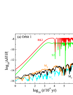
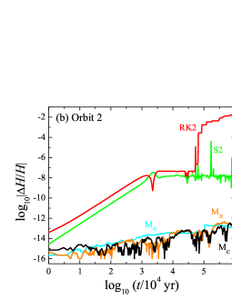
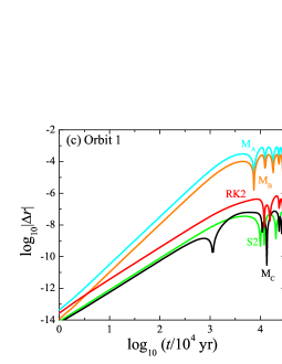
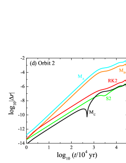
Figure 1: (a) and (b): Relative Hamiltonian errors for five methods. The initial conditions and parameters of two orbits are $H=450$, $b=1$, $\lambda=y=0$, $x=3$, $z=0.1$, and $p_{x}=p_{z}=0$. The other parameters are $\alpha=1$ and $M_{n}=10$ for Orbit 1, while $\alpha=0.1$ and $M_{n}=400$ for Orbit 2. In the accuracy of the Hamiltonian, Method S2 is better than Method RK2 and remains bounded; the three energy-conversing methods $M_{A}$, $M_{B}$ and $M_{C}$ are almost the consistently best. (c) and (d): Absolute position errors for the five methods. $M_{A}$ and $M_{B}$ have almost the same accuracies in the positions, and $M_{C}$ and S2 do. The accuracy for $M_{C}$ is several orders of magnitude better than that for $M_{B}$. This shows that $M_{B}$ gives a first-order accuracy to the numerical solutions, and $M_{C}$ yields a second-order accuracy.

At first, we take parameter $\lambda=0$ and select two different orbits whose initial conditions are $H=450$, $b=1$, $y=p_{x}=p_{z}=0$, $x=3$, and $z=0.1$. Parameters $\alpha=1$ and $M_{n}=10$ for Orbit 1, while $\alpha=0.1$ and $M_{n}=400$ for Orbit 2. The initial values of $p_{y}>0$ of the two orbits are given by Equation (10). The dimensionless time-step takes $h=10^{4}/10^{8}$, which corresponds to a real physical time of $10^{4}$ years. Figures 1 (a) and (b) plot the relative Hamiltonian errors when the five algorithms act on Orbits 1 and 2 to $10^{10}$ years (corresponding to $10^{6}$ steps of integrations). Methods $M_{A}$, $M_{B}$ and $M_{C}$ have approximately same energy errors. These errors are relatively small and slowly grow up to an order of $10^{-13}$ due to roundoff errors. The three integrators should be energy-conserving if the roundoff errors are negligible. RK2 remains bounded in errors for Orbit 1 in Figure 1(a), but does not for Orbit 2 in Figure 1(b). S2 always gives bounded errors to Orbits 1 and 2 because of its symplecticity. RK2 exhibits the largest errors, whereas $M_{A}$, $M_{B}$ and $M_{C}$ yield the smallest errors. In particular, the Hamiltonian errors for $M_{A}$, $M_{B}$ and $M_{C}$ seem to be independent of the choice of Orbit 1 or Orbit 2. However, the position errors for the new method $M_{C}$ in Figures 1 (c) and (d) are almost the same as those for the second-order methods RK2 and S2, and the position errors for Method $M_{B}$ are approximate to those for Method $M_{A}$. The position errors for $M_{C}$, RK2 and S2 are smaller than those for $M_{A}$ and $M_{B}$.

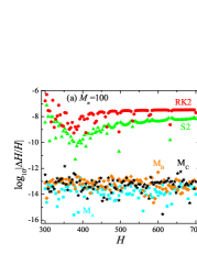
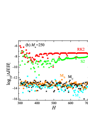
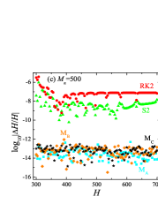
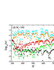
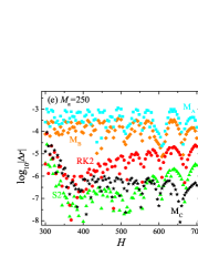
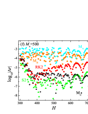
Figure 2: (a)-(c): Dependence of relative Hamiltonian errors on the Hamiltonian $H$ for three values of mass parameter $M_{n}$. (d)-(f): Dependence of absolute position errors on the Hamiltonian. The other parameters are $\lambda=0.001$ and $\alpha=b=1$, and the initial conditions are those of Orbit 1. Each error is obtained after $10^{5}$ integration steps. $M_{A}$, $M_{B}$ and $M_{C}$ have almost the consistently best performance in the Hamiltonian errors, and S2 is better than RK2. On the other hand, $M_{C}$ and S2 are drastically superior to $M_{A}$ and $M_{B}$ in the accuracies of the solutions. This shows again that $M_{B}$ and $M_{C}$ have the same performance in the conservation of energy, but do not have in the accuracies of the solutions.

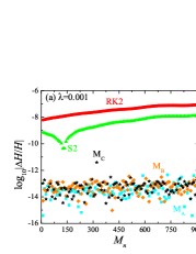
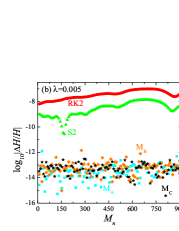
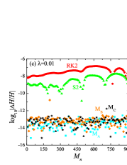
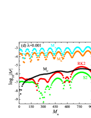
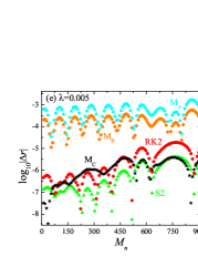
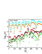
Figure 3: (a)-(c): Dependence of relative Hamiltonian errors on mass parameter $M_{n}$ for three values of parameter $\lambda$. (d)-(f): Dependence of absolute position errors on mass parameter $M_{n}$. The other parameters are $H=400$ and $\alpha=b=1$, and the initial conditions are those of Orbit 1. The performances of $M_{A}$, $M_{B}$ and $M_{C}$ in the Hamiltonian errors are approximately the same as those in Figures 1 and 2. So are the performances of $M_{B}$ and $M_{C}$ in the accuracies of the solutions.

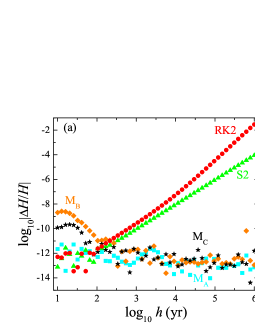
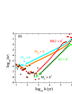
Figure 4: (a): Dependence of relative Hamiltonian errors on time steps $h$. (b): Dependence of absolute position errors on time steps $h$. The parameters are $H=400$, $M_{n}=200$, $\alpha=1.6$, $b=0.8$, and $\lambda=0$. The initial conditions are those of Orbit 1. The integration lasts $10^{10}$ years for each time step. The time steps run from 10 years to $10^{6}$ years; equivalently, the dimensionless time steps are from $10^{-7}$ to $10^{-2}$. Obviously, the position errors of $M_{A}$ and $M_{B}$ grow linearly with the time-step $h$, while those of $M_{C}$, RK2, and S2 grow with $h^{2}$. This sufficiently shows that $M_{A}$ and $M_{B}$ are only accurate to a first-order accuracy to the solutions, and $M_{C}$, RK2, and S2 are accurate to a second-order accuracy.

The dependence of relative Hamiltonian error $\Delta H/H$ on Hamiltonian $H$ in Figures 2 (a)-(c) shows that the Hamiltonian errors among the three schemes $M_{A}$, $M_{B}$ and $M_{C}$ have no dramatic differences, and are several orders of magnitude smaller than S2 or RK2 for different choices of mass parameter $M_{n}$. On the other hand, the absolute position errors for $M_{A}$ are almost consistent with those for $M_{B}$, but are two or three orders of magnitude larger than for the methods S2 and $M_{C}$ in Figures 2 (d)-(f). These results are still supported in Figure 3 that describes the dependence of the relative Hamiltonian error (or the absolute position error) on the mass parameter $M_{n}$ for different choices of parameter $\lambda$. The error trends with an increase of time step in Figure 4 describe that the relative Hamiltonian errors for RK2 are slightly larger than those for S2, but are relatively larger than those for anyone of Methods $M_{A}$, $M_{B}$ and $M_{C}$. The relative Hamiltonian errors increase with an increase of time step for RK2 and S2, whereas are independent of any choice of time steps for $M_{A}$, $M_{B}$ and $M_{C}$. On the other hand, the absolute position errors grow with an increase of dimensionless time step $h>1/100000$ for the five methods. In particular, the rules of the growth of absolute position error with time step $h$ for the these algorithms are $\Delta r\propto h$ for $M_{A}$ and $M_{B}$, and $\Delta r\propto h^{2}$ for $M_{C}$, S2 and RK2. Clearly, $M_{C}$ with S2 has the smallest position errors for dimensionless time steps $10^{-5}\leq h\leq 10^{-3}$.

In short, the numerical results in Figures 1-4 have sufficiently conformed that the schemes $M_{A}$, $M_{B}$ and $M_{C}$ can conserve energy if the roundoff errors are neglected. They are also greatly superior to the second-order symplectic method S2 in conservation of energy. However, the three energy-conserving schemes are different in accuracy of the solutions. $M_{A}$ and $M_{B}$ have almost the same position errors. $M_{C}$ with S2 has, too. Particular for dimensionless time steps $10^{-5}\leq h\leq 10^{-3}$, $M_{C}$ and S2 give the best accuracy to the solutions. In other words, the numerical tests have supported that $M_{B}$ yields a first-order accuracy to the numerical solutions and $M_{C}$ has a second-order accuracy.

3.3 Dynamics of orbits

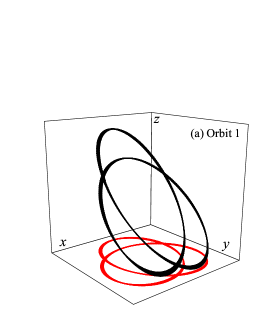
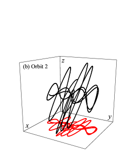
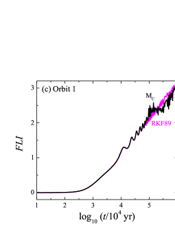
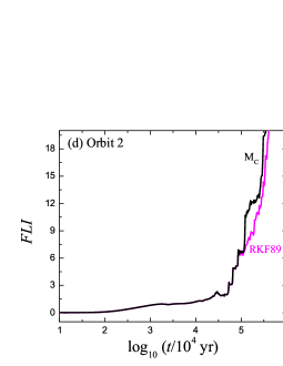
Figure 5: (a) and (b): Two orbits in Figure 1 are shown in the three-dimensional space. The red curves represent the projection of the trajectories on the $xoy$-plane. (c) and (d): Fast Lyapunov indicators (FLIs) for Orbits 1 and 2. Methods $M_{C}$ and RKF89 give almost the same values of the FLIs. The FLI for Orbit 1 is much smaller than that for Orbit 2. Orbit 1 is regular, whereas Orbit 2 is chaotic.

Considering that Method $M_{C}$ with an optimal time step (such as $h=10^{-4}$) shows better performance in conservation of energy and accuracy of solutions, we apply it to give some insight into the dynamical behavior of orbits. Seen from Figures 5 (a) and (b), the two orbits seem to have distinct three-dimensional configurations. Orbit 1 in Figure 5(a) seems to be periodic or quasi-periodic, but Orbit 2 in Figure 2(b) seems to be chaotic. These results are not shown through the method of Poincaré-sections/maps because the phase space has six dimensions, but can be confirmed by fast Lyapunov indicators (FLIs) in Figures 5 (c) and (d). Here, the FLIs are calculated in terms of the two-particle method (Wu et al. 2006). Different time rates of the growth of FLIs are used to identify the regular or chaotic behavior. A bounded orbit is ordered when its FLI grows algebraically with time, but chaotic if its FLI increases exponentially. Based on this criterion, the regularity of Orbit 1 and the chaoticity of Orbit 2 are clearly identified. The results of Method $M_{C}$ are consistent with those of the high-precision algorithm RKF89.

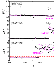
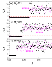
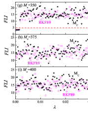
Figure 6: Dependence of FLI on parameter $\lambda$ under the circumstance of different galaxy masses $M_{n}$. $H=400$, $\alpha=1.6$, and $b=0.8$. Each of the FLIs is obtained after $3\times 10^{5}$ integration steps. The FLIs larger than 5 indicate the chaoticity; the FLIs less than 5 indicate the regularity. For $M_{n}=200$ in (a), all values of $\lambda\in[0,0.03]$ correspond to order. For $M_{n}=225$ in (b), chaos occurs when $\lambda\geq 0.0255$. For $M_{n}=250$, $275$, $300$, $325$, and $350$ in (c)-(g), the critical values $\lambda$ for inducing chaos are 0.0192, 0.0138, 0.009, 0.0048, and 0.0018, respectively. For $M_{n}=375$, and $400$, all values of $\lambda\in[0,0.03]$ correspond to chaos. These facts show that chaos easily occurs when $M_{n}$ increases, but the critical value of $\lambda$ for the occurrence of chaos decreases with an increase of $M_{n}$.

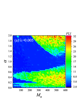
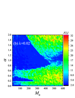
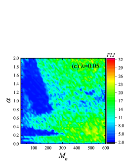
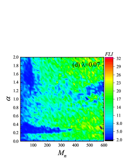
Figure 7: Finding chaos by using the FLIs to scan a two-dimensional space of parameters $\alpha$ and $M_{n}$. Other parameters are $H=400$ and $b=1$. Chaotic regions in the parameter space of $\alpha$ and $M_{n}$ get larger as $M_{n}$ and $\lambda$ increase.

Using the technique of FLIs, we trace the effects of varying the parameters on the occurrence of chaos. The initial conditions are still those in Figure 1, and parameters $H=400$, $\alpha=1.6$, and $b=0.8$ are always fixed. Mass $M_{n}$ is given several values, and $\lambda$ ranges from 0 to 0.03 with an interval of $3\times 10^{-4}$. For each value of $\lambda$, the FLI is obtained after $3\times 10^{5}$ integration steps. In this way, the relation between the FLI and $\lambda$ is described in Figure 6. 5 is found to be a threshold of FLIs between order and chaos. The values of $\lambda$ with $FLI\geq 5$ correspond to the chaoticity, whereas the values of $\lambda$ with $FLI<5$ indicate the regularity. Figure 6 relates to the description of finding chaos by scanning a space of parameter $\lambda$; in fact, this figure establishes a correspondence between parameter $\lambda$ and chaos or order. It is shown clearly in Figure 6 that a transition from order to chaos easily occurs as parameter $\lambda$ increases. If $\lambda$ is given, the presence of chaos also becomes easier with an increase of mass $M_{n}$. Particularly for a larger value of $M_{n}$ in Figures 6 (h) and (i), all values of $\lambda$ indicate chaos. These dynamical results of order and chaos obtained from Method $M_{C}$ are in perfect agreement with those given by RKF89. Scanning a two-dimensional space of parameters $\alpha$ and $M_{n}$ in Figure 7 shows that the occurrence of chaos is difficult when the values of $\alpha$ are in the neighbourhood of 1, but it is easy when the values of $\alpha$ are far away from 1. The effect of varying the parameter $b$ on the presence of chaos should be similar to that of varying the parameter $\alpha$. The effects of varying the parameters on the presence of chaos in the present paper are the same as those of Zotos (2014).

An explanation to the dependence of chaos on the parameters is given here. A larger value of perturbation parameter $\lambda$ or mass $M_{n}$ means strengthening the gravity of BL Lac objects in Equations (10)-(12), therefore, there is a more chance of chaos. For $\alpha\approx 1$ in Equation (11), the potential of the elliptical galaxy tends to the isotropy with respect to the three axes in the case of $b=1$. However, the potential destroys the isotropy for $\alpha$ far away from 1. As a result, chaos is easily present.

4 Magnetized rotating black hole

By analyzing the motion of charged particles around a black hole, one can understand the spacetime properties around the black hole and test the general theory of relativity. In addition, the motion of charged particles reflects the evolution of the accretion disk around the black hole, and is useful to understand the accretion process of the black hole. Because of this, the dynamics of charged particles moving around a rotating black hole in an external magnetic field was considered in the work of Kopáček $\&$ Karas (2014). Now, the dynamical model is used to evaluate the above-mentioned algorithms. The dynamics of charged particles is further surveyed.

4.1 Dynamical model

In Boyer-Lindquist coordinates $x^{\mu}=(t,r,\theta,\varphi)$, the Kerr metric is expressed as (Misner et al. 1973)

$$\textrm{d}s^{2} = \frac{\Sigma}{\Delta}\textrm{d}r^{2}+\Sigma\textrm{d}\theta^{2}-\frac{\Delta}{\Sigma}[\textrm{d}t-a\textrm{sin}\theta\textrm{d}\varphi]^{2}$$ (13)

$$+\frac{\textrm{sin}^{2}\theta}{\Sigma}[(r^{2}+a^{2})\textrm{d}\varphi-a\textrm{d}t]^{2},$$

where $a$ stands for the spin parameter (i.e., the specific angular momentum) of the Kerr black hole with mass $M$, $\Sigma$ and $\Delta$ are written as follows:

$$\Delta = r^{2}-2Mr+a^{2},$$ (14)

$$\Sigma = r^{2}+a^{2}\textrm{cos}^{2}\theta.$$ (15)

Gravitational constant $G$ and speed of light $c$ take geometrized units: $c=G=1$.

Kopác̆ek $\&$ Karas (2014) assumed that the rotating black hole has a non-zero electric charge $Q$. Although such a black hole is the Kerr-Newman black hole in this case, the electromagnetic field generated by the black hole’s electric charge is so weak that it does not affect the spacetime and plays an important role in the motion of charged particles around the black hole. Because of this, the metric still remains unaltered by $Q$. They also considered that the rotating Kerr black hole is immersed in an asymptotically uniform magnetic field with the vector potential:

$$A_{t} = \frac{aB_{z}Mr}{\Sigma}(1+\textrm{cos}^{2}\theta)-aB_{z}-\frac{Qr}{\Sigma}$$ (16)

$$+\frac{aMB_{x}\textrm{sin}\theta\textrm{cos}\theta}{\Sigma}(r\textrm{cos}\psi-a\textrm{sin}\psi),$$

$$A_{r} = -B_{x}(r-M)\textrm{cos}\theta\textrm{sin}\theta\textrm{sin}\psi,$$ (17)

$$A_{\theta} = -B_{x}(r^{2}\textrm{cos}^{2}\theta-Mr\textrm{cos}2\theta+a^{2}\textrm{cos}2\theta)\textrm{sin}\psi$$ (18)

$$-aB_{x}(r\textrm{sin}^{2}\theta+M\textrm{cos}^{2}\theta)\textrm{cos}\psi,$$

$$A_{\varphi} = B_{z}\sin^{2}\theta\left[\frac{1}{2}(r^{2}+a^{2})-\frac{a^{2}Mr}{\Sigma}(1+\cos^{2}\theta)\right]$$ (19)

$$-B_{x}\sin\theta\cos\theta\left[\Delta\cos\psi+\frac{(r^{2}+a^{2})M}{\Sigma}\right.$$

$$\left.\cdot(r\cos\psi-a\sin\psi)\right]+\frac{Qar\sin^{2}\theta}{\Sigma}.$$

This magnetic field was derived by Wald (1974) and generalized by Bičák $\&$ Janiš (1985). Here, $B_{x}$ and $B_{z}$ are constant magnetic parameters, $\psi$ and $r_{\pm}$ read as

$$\psi = \varphi+\frac{a}{r_{+}-r_{-}}\ln\frac{r-r_{+}}{r-r_{-}},$$ (20)

$$r_{\pm} = M\pm\sqrt{M^{2}-a^{2}}.$$ (21)

The dynamics of a test particle with charge $q$ and mass $m$ moving around the black hole with external magnetic field can be described by the following super-Hamiltonian

$$\mathcal{H}=\frac{1}{2m}g^{\mu\nu}(p_{\mu}-qA_{\mu})(p_{\nu}-qA_{\nu}),$$ (22)

where the particle’s generalized momenta $p_{\mu}=mg_{\mu\nu}\dot{x}^{\nu}+qA_{\mu}$. Its canonical equations are

$$\dot{t} = \frac{\partial\mathcal{H}}{\partial p_{t}}$$ (23)

$$= g^{tt}(p_{t}-qA_{t})+g^{t\varphi}(p_{\varphi}-qA_{\varphi}),$$

$$\dot{p_{t}} = -\frac{\partial\mathcal{H}}{\partial t}=0;$$ (24)

$$\dot{r} = \frac{\partial\mathcal{H}}{\partial p_{r}},~{}~{}~{}~{}\dot{\theta}=\frac{\partial\mathcal{H}}{\partial p_{\theta}},~{}~{}~{}~{}\dot{\varphi}=\frac{\partial\mathcal{H}}{\partial p_{\varphi}},$$ (25)

$$\dot{p_{r}} = -\frac{\partial\mathcal{H}}{\partial r},~{}\dot{p_{\theta}}=-\frac{\partial\mathcal{H}}{\partial\theta},~{}\dot{p_{\varphi}}=-\frac{\partial\mathcal{H}}{\partial\varphi}.$$ (26)

Equation (24) shows that the conjugate momentum $p_{t}$ is a constant of motion and is related to energy $E$ of the test particle, namely, $p_{t}=-E$. Another constant is

$$\mathcal{H}=-\frac{m}{2}.$$ (27)

Other constants like the particle’s angular momentum are no longer present due to the magnetic field governed by parameter $B_{x}$ breaking axial symmetry. In this sense, the super-Hamiltonian is a six-dimensional nonintegrable system, whose evolution is dominated by Equations (25) and (26).

For simplicity, scale transformations are used as dimensionless operations to the super-Hamiltonian. The operations are as follows: $r\rightarrow rM$, $t\rightarrow tM$, $\tau\rightarrow\tau M$, $a\rightarrow aM$, $Q\rightarrow QM$, $E\rightarrow Em$, $p_{r}\rightarrow mp_{r}$, $p_{\varphi}\rightarrow mMp_{\varphi}$, $p_{\theta}\rightarrow mMp_{\theta}$, $q\rightarrow mq$, $B_{x}\rightarrow B_{x}/M$, $B_{z}\rightarrow B_{z}/M$ and $\mathcal{H}\rightarrow m\mathcal{H}$. As a result, $M\rightarrow 1$ in the above expressions, and the black hole’s angular momentum satisfies $|a|\leq 1$. In addition, $\mathcal{H}=-1/2$ and $|Q|\leq 1$.

4.2 Numerical investigations

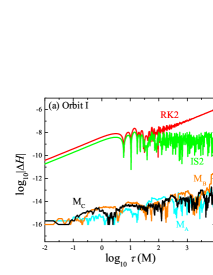
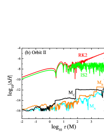
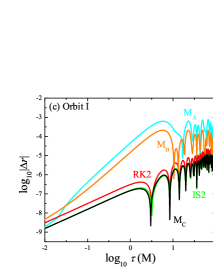
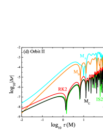
Figure 8: Errors in the Hamiltonian and solutions in the magnetized black hole background. The numerical performances of the five algorithms in the errors of the Hamiltonian and solutions are similar to those in Figure 1.

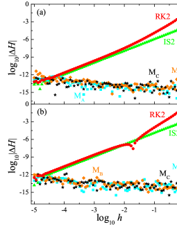
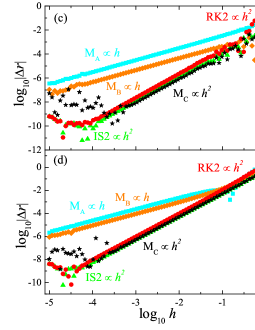
Figure 9: Relations between the time steps $h$ and the errors in the Hamiltonian and solutions. (a) and (c): Orbit I. (b) and (d): Orbit II. Each error is obtained after the integration time $\tau=100$. Panels (c) and (d) show that the position errors of $M_{A}$ and $M_{B}$ grow linearly with $h$, while those of $M_{C}$, RK2, and S2 grow with $h^{2}$. This implies that $M_{A}$ and $M_{B}$ are first-order schemes, and $M_{C}$, RK2, and S2 are second-order schemes. The result is consistent with that in Figure 4.

Let us consider two orbits with same initial values $p_{r}=p_{\varphi}=0$ and charge $q=1$. Orbit I has other initial conditions $r=3.9$, $\theta=1.15$, $\varphi=0$ and $L=p_{\varphi}=6$, and parameters $a=0.9$, $Q=1$, $E=1.61$, $B_{x}=0.001$ and $B_{z}=1$. Orbit II has other initial conditions $r=5$, $\theta=1$, $\varphi=\pi/3$ and $L=5.6$, and parameters $a=0.8$, $Q=0.5$, $E=1.325$, $B_{x}=0.007$ and $B_{z}=0.7$. The time step is $h=0.01$. The second-order explicit symplectic algorithm (S2) is replaced by the second-order midpoint implicit symplectic method (IS2). Figure 8 supports that the three energy-conserving schemes have same good effects on Hamiltonian conservations, compared with the methods RK2 and IS2. However, Method $M_{C}$ is basically the same as the second-order methods IS2 and RK2, and Method $M_{B}$ is similar to the first-order method $M_{A}$ in accuracy of the solutions. This shows again that $M_{B}$ gives a first-order accuracy to the numerical solutions, and $M_{C}$ possesses a second-order accuracy. These results are also confirmed in Figure 9 that describes the dependence of the errors on the time steps. Good choices of time steps are from $h\sim 10^{-3}$ to $h\sim 10^{-2}$.

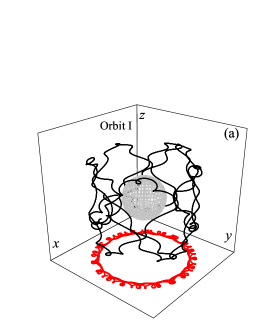
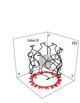
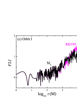
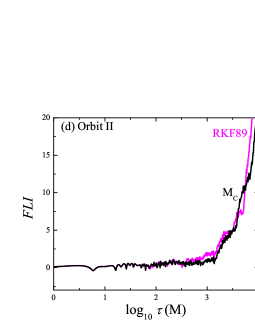
Figure 10: (a) and (b): Two orbits in Figure 8 are plotted in the three-dimensional space. The red curves represent the projection of the trajectories on the $xoy$-plane. (c) and (d): Growth of fast Lyapunov indicators (FLIs) with proper time $\tau$ for Orbits I and II. Orbit I is ordered, but Orbit II is chaotic.

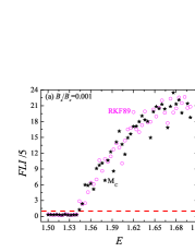
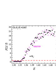
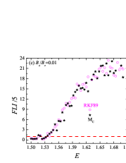
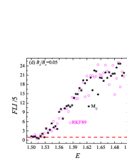
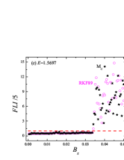
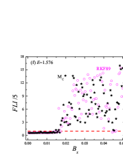
Figure 11: (a)-(d): Dependence of FLI on energy $E$. The initial conditions and other parameters are $a=0.75$, $L=6$, $Q=1$, $B_{z}=1$, $r=4$, $\theta=1$, $\varphi=p_{r}=0$. Each of the FLIs is obtained after $5\times 10^{5}$ integration steps. The plotted FLIs are a fifth of the real FLIs. The plotted FLIs larger than 1 indicate the chaoticity; the plotted FLIs less than 1 indicate the regularity. Chaos occurs for $E\geq 1.544$ in (a), $E\geq 1.54$ in (b), $E\geq 1.536$ in (c), and $E\geq 1.52$ in (d). This indicates that a smaller energy easily induces chaos for a larger value of $B_{x}$. In other words, the onset of chaos becomes easier as $E$ and $B_{x}$ get larger. (e) and (f): Dependence of FLIs on magnetic field parameter $B_{x}$. The parameters and initial conditions different from those in (a)-(d) are $a=0.8$, $L=5$, $r=3.66$, and $\theta=\pi/2$. Chaos occurs for $B_{x}\geq 0.03416$ in (e), and $B_{x}\geq 0.01486$ in (f). This means that an increase of $B_{x}$ easily leads to the onset of chaos.

Now, Method $M_{C}$ with the appropriate time step $h=10^{-2}$ is applied to study the long-term evolution of orbits. Orbits I and II have different three-dimensional configurations in Figures 10 (a) and (b). The FLIs in Figures 10 (c) and (d) indicate the regularity of Orbit I and the chaoticity of Orbit II. The results of the FLIs for Method $M_{C}$ are completely consistent with those for RKF89. The effects of varying energies $E$ on the FLIs in Figures 11 (a)-(d) show that chaos easily occurs as the energy $E$ increases. In addition, an increase of $B_{x}$ with $B_{z}=1$ causes a smaller energy to induce chaos. The result is consistent with that of Kopáček $\&$ Karas (2014). Here, the FLI for each value of $E$ is obtained after $5\times 10^{5}$ integration steps. The energies with FLIs $<$ 5 correspond to the regularity, but those with FLIs $\geq$ 5 indicate the onset of strong chaos. Chaos occurs for $E\geq 1.544$ with $B_{x}=0.001$ [Figure 11(a)], $E\geq 1.54$ with $B_{x}=0.005$ [Figure 11(b)], $E\geq 1.536$ with $B_{x}=0.01$ [Figure 11(c)], and $E\geq 1.52$ with $B_{x}=0.05$ [Figure 11(d)]. To clearly show the dependence of the orbital dynamical behavior on a variation of magnetic field parameter $B_{x}$, we plot Figures 11 (e) and (f), where another magnetic field parameter $B_{z}=1$ is fixed. Chaos occurs for $B_{x}\geq 0.03416$ with $E=1.5697$ [Figure 11(e)], and $B_{x}\geq 0.01486$ with $E=1.576$ [Figure 11(f)]. This shows that magnetic field parameter $B_{x}$ has a critical value, which makes the dynamics transit from order to chaos. In fact, this value is closely related to $E$. These results clearly describe the above-mentioned dependence of the dynamical transition from order to chaos with an increase of energy or magnetic field parameter $B_{x}$.

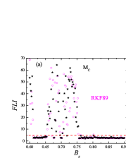
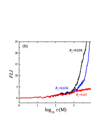
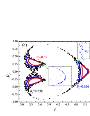
Figure 12: (a): Dependence of FLIs on magnetic field parameter $B_{z}$. The other parameters and initial conditions are $B_{x}=0$, $a=0.8$, $E=1.48$, $L=5$, $Q=1$, $r=3.5$, $\theta=1$, and $\varphi=0$. Each of the FLIs is obtained after $5\times 10^{5}$ integration steps. The red dashed line is the boundary between the FLIs of regularity and chaoticity. The values of $B_{z}$ are [0.612, 0.654] and [0.756, 0.9] for the regular case, and [0.6, 0.61], [0.656, 0.659] for the chaotic case. (b): Growth of FLIs with proper time $\tau$ for three values of $B_{z}$: 0.65, 0.656 and 0.658. The FLIs increase when $B_{z}$ runs from 0.65 to 0.658. (c): Poincaré-sections/maps at plane $\theta=\pi/2$ with $p_{\theta}>0$ for the three values of $B_{z}$. The three values of $B_{z}$ 0.65, 0.656 and 0.658 correspond to regularity, weak chaoticity and strong chaoticity, respectively. For the case of $B_{x}=0$, the angular momentum $L$ is a constant. Therefore, the motions are restricted to a 4-dimensional phase space $r$, $\theta$, $p_{r}$ and $p_{\theta}$.

One of the results concluded from Figure 11 is that chaos can occur for a smaller energy as $B_{x}$ with $B_{z}=1$ increases. What about the dynamical transition from order to chaos with a variation of $B_{z}$? Figure 12(a) answers this question. Here, we take the initial conditions $r=3.5$, $\theta=1$ and $\varphi=0$ and the parameters $B_{x}=0$, $a=0.8$, $E=1.48$, $L=5$ and $Q=1$, and let $B_{z}$ range from 0.6 to 0.9 with an interval of 0.002. Regular regions of $B_{z}$ are [0.612, 0.654] and [0.756, 0.9], and chaotic regions of $B_{z}$ are [0.6, 0.61] and [0.656, 0.696]. Clearly, a dynamical transition from order to chaos occurs in the vicinity of $B_{z}=0.65$. The FLIs for three values of $B_{z}$ in Figure 12(b) explicitly show that the regularity exists for $B_{z}=0.65$, and chaos for $B_{z}=0.656$ is weaker than for $B_{z}=0.658$. The Poincaré sections in Figure 12(c) display that $B_{z}=0.65$ corresponds to three islands of the regularity (i.e., a resonance), whereas $B_{z}=0.658$ leads to losing the three islands and a number of discrete points filled with a small area, i.e., the chaotic behavior. The orbit for $B_{z}=0.656$, located in a sepratrix location between the regular islands and the chaotic layers, seems to be three islands of the regularity, but consists of three thin chaotic layers. That is, $B_{z}$=0.65, 0.656 and 0.658 correspond to order, weak chaos, and strong chaos, respectively. This chaoticity in Figures 10-12 is due to external perturbations from the magnetic field forces governed by parameters $B_{x}$ and/or $B_{z}$. Given $B_{x}=B_{z}=0$, Equation (22) is the Kerr-Newman black hole (13), which is integrable and nonchaotic. However, the magnetic field forces for $B_{x}\neq 0$ and/or $B_{z}\neq 0$ cause Equation (22) to be nonintegrable. When the magnetic field forces are small, the motions are mainly dominated by the gravity from the black hole and are still regular Kolmogorov-Arnold-Moser (KAM) tori. In spite of the regularity, these tori are twisted by the external perturbations. As the external perturbations get stronger, some tori are destroyed and departures from stability and resonances appear. When the black hole’s gravity basically matches with the magnetic field forces, chaos occurs. This is just an example shown in Figure 12(c). Now, we explain why the technique of Poincaré-sections/maps can be used in Figure 12 but cannot in Figures 10 and 11. For the case of $B_{x}=0$ in Figure 12, the angular momentum $L=g_{t\varphi}\dot{t}+g_{\varphi\varphi}\dot{\varphi}+qA_{\varphi}$ is conserved. Thus, all orbits are restricted to a 4-dimensional phase space made of $r$, $\theta$, $p_{r}$ and $p_{\theta}$, and the technique of Poincaré-sections/maps can work well. For the case of $B_{x}\neq 0$ in Figures 10 and 11, $L$ varies with time. Therefore, all motions are in the 6-dimensional phase space made of $r$, $\theta$, $\varphi$, $p_{r}$, $p_{\theta}$, and $p_{\varphi}$, and the technique of Poincaré-sections/maps is not suitable for this case. Because $B_{x}$ destroys the conservation of the angular momentum $L$ but $B_{z}$ does not, $B_{x}$ and $B_{z}$ exert different influences on the chaotic behavior. That is, an increase of $B_{x}$ breaks the axial symmetry and strengthens the chaotic properties in Figures 11 (e) and (f), but that of $B_{z}$ does not always strengthen in Figure 12(a).

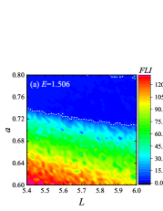
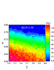
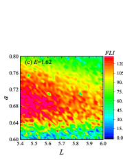
Figure 13: Finding chaos by using the FLIs to scan a two-dimensional space of parameter $a$ and the initial angular momentum $L$. $B_{z}=1$ and $B_{x}=0.001$. The white dashed line corresponds to $FLI=5$, which is the boundary between the chaotic and ordered regions. Strong chaos exists for smaller values of $a$ and $L$ in (a) and (b), but it does for $a\in[0.64,0.77]$ in (c).

For $B_{x}\neq 0$ and $B_{z}\neq 0$, Figure 13 shows that a smaller initial angular momentum $L$ of the particle easily yields chaos. The strength of chaos is not always enhanced or weakened as the black hole’s angular momentum $a$ increases. In fact, chaos is stronger for $0.6\leq a\leq 0.64$ with $5.4\leq L\leq 5.6$, but is absent for $0.76\leq a\leq 0.8$ with any initial angular momenta $L$ in Figure 13(a). Chaos is stronger for $0.6\leq a\leq 0.68$ with $5.4\leq L\leq 5.7$, but is absent for $0.78\leq a\leq 0.8$ with any initial angular momenta $L$ in Figure 13(b). Although chaos is present for all values of $a$ and $L$ considered in Figure 13(c), stronger chaos occurs for $0.64\leq a\leq 0.76$. The result is not completely consistent with that of Takahashi $\&$ Koyama (2009) on the black hole spin weakening the chaotic properties. This is due to different combinations of initial conditions and other dynamical parameters. There is no universal rule on the relation between the dynamical transition and the black hole spin (Sun et al. 2021).

5 Summary

It is shown analytically that the existing six-dimensional Hamiltonian-conserving algorithm of Bacchini et al. (2018) does not possess a second-order accuracy to numerical solutions, but has a first-order accuracy only. A new second-order six-dimensional Hamiltonian-conserving scheme is proposed. Taking the Galactic model hosting a BL Lacertae object and the dynamics of charged particles moving around a rotating black hole in an external magnetic field as test models, we numerically confirm that the existing method of Bacchini et al and the newly proposed scheme are energy-conserving, but have different performances in accuracy of the numerical solutions. The numerical solutions are accurate to first order for the former scheme, but to second order for the latter method.

The new energy-conserving method combined with appropriate time steps is used to explore the effects of varying the parameters on the presence of chaos in the two physical models. Chaos easily occurs in the Galactic model as the mass of the nucleus, the internal perturbation parameter, and the anisotropy of the potential of the elliptical galaxy increase. Larger energies of the particles, smaller initial initial angular momenta of the particles, and stronger magnetic fields (that are mainly governed by parameter $B_{x}$) are helpful to induce chaos in the magnetized Kerr spacetime. The chaotic properties are not necessarily weakened when the black hole spin increases.

The new scheme has no symplecticity. However, it is time reversibility as a property of some particular symplectic problems, and it has also excellent energy conservation. Because of the time reversibility, the new method including the particular symplectic problems is suitable for tracing the origin and evolution of some celestial objects. The new second-order energy-conserving method involving a second order symplectic integrator with appropriately smaller steps can achieve similar accuracies of high-order symplectic partitioned Runge-Kutta methods with correspondingly larger time steps. It can also take less computational cost, compared to the high-order methods. Based on these facts, a second-order symplectic integrator is often used as very long-time integrations of celestial objects, for example, $N$-body problems in the solar system (Wisdom $\&$ Holman 1991). The new scheme can be used for any six-dimensional Hamiltonian problems, including globally hyperbolic spacetimes with readily available (3+1) split coordinates. These spacetimes are, e.g., the Kerr metric and the Kerr black hole with external magnetic fields.

Appendix

Appendix A Simple discrete method of the derivatives

$$\frac{q_{1}^{n+1}-q_{1}^{n}}{h} = \frac{1}{p_{1}^{n+1}-p_{1}^{n}}\left[H(q_{1}^{n},q_{2}^{n},q_{3}^{n},p_{1}^{n+1},p_{2}^{n},p_{3}^{n})\right.\left.-H(q_{1}^{n},q_{2}^{n},q_{3}^{n},p_{1}^{n},p_{2}^{n},p_{3}^{n})\right],$$ (A1)

$$\frac{q_{2}^{n+1}-q_{2}^{n}}{h} = \frac{1}{p_{2}^{n+1}-p_{2}^{n}}\left[H(q_{1}^{n},q_{2}^{n},q_{3}^{n},p_{1}^{n+1},p_{2}^{n+1},p_{3}^{n})\right.\left.-H(q_{1}^{n},q_{2}^{n},q_{3}^{n},p_{1}^{n+1},p_{2}^{n},p_{3}^{n})\right],$$ (A2)

$$\frac{q_{3}^{n+1}-q_{3}^{n}}{h} = \frac{1}{p_{3}^{n+1}-p_{3}^{n}}\left[H(q_{1}^{n},q_{2}^{n},q_{3}^{n},p_{1}^{n+1},p_{2}^{n+1},p_{3}^{n+1})\right.\left.-H(q_{1}^{n},q_{2}^{n},q_{3}^{n},p_{1}^{n+1},p_{2}^{n+1},p_{3}^{n})\right],$$ (A3)

$$\frac{p_{1}^{n+1}-p_{1}^{n}}{h} = -\frac{1}{q_{1}^{n+1}-q_{1}^{n}}\left[H(q_{1}^{n+1},q_{2}^{n},q_{3}^{n},p_{1}^{n+1},p_{2}^{n+1},p_{3}^{n+1})\right.\left.-H(q_{1}^{n},q_{2}^{n},q_{3}^{n},p_{1}^{n+1},p_{2}^{n+1},p_{3}^{n+1})\right],$$ (A4)

$$\frac{p_{2}^{n+1}-p_{2}^{n}}{h} = -\frac{1}{q_{2}^{n+1}-q_{2}^{n}}\left[H(q_{1}^{n+1},q_{2}^{n+1},q_{3}^{n},p_{1}^{n+1},p_{2}^{n+1},p_{3}^{n+1})\right.\left.-H(q_{1}^{n+1},q_{2}^{n},q_{3}^{n},p_{1}^{n+1},p_{2}^{n+1},p_{3}^{n+1})\right],$$ (A5)

$$\frac{p_{3}^{n+1}-p_{3}^{n}}{h} = -\frac{1}{q_{3}^{n+1}-q_{3}^{n}}\left[H(q_{1}^{n+1},q_{2}^{n+1},q_{3}^{n+1},p_{1}^{n+1},p_{2}^{n+1},p_{3}^{n+1})\right.\left.-H(q_{1}^{n+1},q_{2}^{n+1},q_{3}^{n},p_{1}^{n+1},p_{2}^{n+1},p_{3}^{n+1})\right].$$ (A6)

Appendix B Existing complex discrete method of the derivatives

The discrete equations (39)-(44) with respect to Equations (2) and (3) in the work of Bacchini et al. (2018) are written as follows:

$$\frac{q_{1}^{n+1}-q_{1}^{n}}{h} = \frac{1}{6(p_{1}^{n+1}-p_{1}^{n})}\{[H(q_{1}^{n+1},q_{2}^{n},q_{3}^{n},p_{1}^{n+1},p_{2}^{n},p_{3}^{n})-H(q_{1}^{n+1},q_{2}^{n},q_{3}^{n},p_{1}^{n},p_{2}^{n},p_{3}^{n})]$$ (B1)

$$+[H(q_{1}^{n+1},q_{2}^{n+1},q_{3}^{n+1},p_{1}^{n+1},p_{2}^{n+1},p_{3}^{n+1})-H(q_{1}^{n+1},q_{2}^{n+1},q_{3}^{n+1},p_{1}^{n},p_{2}^{n+1},p_{3}^{n+1})]$$

$$+[H(q_{1}^{n},q_{2}^{n+1},q_{3}^{n+1},p_{1}^{n+1},p_{2}^{n+1},p_{3}^{n+1})-H(q_{1}^{n},q_{2}^{n+1},q_{3}^{n+1},p_{1}^{n},p_{2}^{n+1},p_{3}^{n+1})]$$

$$+[H(q_{1}^{n+1},q_{2}^{n},q_{3}^{n+1},p_{1}^{n+1},p_{2}^{n},p_{3}^{n+1})-H(q_{1}^{n+1},q_{2}^{n},q_{3}^{n+1},p_{1}^{n},p_{2}^{n},p_{3}^{n+1})]$$

$$+[H(q_{1}^{n},q_{2}^{n},q_{3}^{n},p_{1}^{n+1},p_{2}^{n},p_{3}^{n})-H(q_{1}^{n},q_{2}^{n},q_{3}^{n},p_{1}^{n},p_{2}^{n},p_{3}^{n})]$$

$$+[H(q_{1}^{n},q_{2}^{n},q_{3}^{n+1},p_{1}^{n+1},p_{2}^{n},p_{3}^{n+1})-H(q_{1}^{n},q_{2}^{n},q_{3}^{n+1},p_{1}^{n},p_{2}^{n},p_{3}^{n+1})]\},$$

$$\frac{q_{2}^{n+1}-q_{2}^{n}}{h} = \frac{1}{6(p_{2}^{n+1}-p_{2}^{n})}\{[H(q_{1}^{n+1},q_{2}^{n+1},q_{3}^{n},p_{1}^{n+1},p_{2}^{n+1},p_{3}^{n})-H(q_{1}^{n+1},q_{2}^{n+1},q_{3}^{n},p_{1}^{n+1},p_{2}^{n},p_{3}^{n})]$$ (B2)

$$+[H(q_{1}^{n},q_{2}^{n+1},q_{3}^{n},p_{1}^{n},p_{2}^{n+1},p_{3}^{n})-H(q_{1}^{n},q_{2}^{n+1},q_{3}^{n},p_{1}^{n},p_{2}^{n},p_{3}^{n})]$$

$$+[H(q_{1}^{n},q_{2}^{n},q_{3}^{n},p_{1}^{n},p_{2}^{n+1},p_{3}^{n})-H(q_{1}^{n},q_{2}^{n},q_{3}^{n},p_{1}^{n},p_{2}^{n},p_{3}^{n})]$$

$$+[H(q_{1}^{n+1},q_{2}^{n+1},q_{3}^{n+1},p_{1}^{n+1},p_{2}^{n+1},p_{3}^{n+1})-H(q_{1}^{n+1},q_{2}^{n+1},q_{3}^{n+1},p_{1}^{n+1},p_{2}^{n},p_{3}^{n+1})]$$

$$+[H(q_{1}^{n+1},q_{2}^{n},q_{3}^{n},p_{1}^{n+1},p_{2}^{n+1},p_{3}^{n})-H(q_{1}^{n+1},q_{2}^{n},q_{3}^{n},p_{1}^{n+1},p_{2}^{n},p_{3}^{n})]$$

$$+[H(q_{1}^{n+1},q_{2}^{n},q_{3}^{n+1},p_{1}^{n+1},p_{2}^{n+1},p_{3}^{n+1})-H(q_{1}^{n+1},q_{2}^{n},q_{3}^{n+1},p_{1}^{n+1},p_{2}^{n},p_{3}^{n+1})]\},$$

$$\frac{q_{3}^{n+1}-q_{3}^{n}}{h} = \frac{1}{6(p_{3}^{n+1}-p_{3}^{n})}\{[H(q_{1}^{n+1},q_{2}^{n+1},q_{3}^{n+1},p_{1}^{n+1},p_{2}^{n+1},p_{3}^{n+1})-H(q_{1}^{n+1},q_{2}^{n+1},q_{3}^{n+1},p_{1}^{n+1},p_{2}^{n+1},p_{3}^{n})].$$ (B3)

$$+[H(q_{1}^{n},q_{2}^{n+1},q_{3}^{n+1},p_{1}^{n},p_{2}^{n+1},p_{3}^{n+1})-H(q_{1}^{n},q_{2}^{n+1},q_{3}^{n+1},p_{1}^{n},p_{2}^{n+1},p_{3}^{n})]$$

$$+[H(q_{1}^{n},q_{2}^{n+1},q_{3}^{n},p_{1}^{n},p_{2}^{n+1},p_{3}^{n+1})-H(q_{1}^{n},q_{2}^{n+1},q_{3}^{n},p_{1}^{n},p_{2}^{n+1},p_{3}^{n})]$$

$$+[H(q_{1}^{n},q_{2}^{n},q_{3}^{n+1},p_{1}^{n},p_{2}^{n},p_{3}^{n+1})-H(q_{1}^{n},q_{2}^{n},q_{3}^{n+1},p_{1}^{n},p_{2}^{n},p_{3}^{n})]$$

$$+[H(q_{1}^{n+1},q_{2}^{n+1},q_{3}^{n},p_{1}^{n+1},p_{2}^{n+1},p_{3}^{n+1})-H(q_{1}^{n+1},q_{2}^{n+1},q_{3}^{n},p_{1}^{n+1},p_{2}^{n+1},p_{3}^{n})]$$

$$+[H(q_{1}^{n},q_{2}^{n},q_{3}^{n},p_{1}^{n},p_{2}^{n},p_{3}^{n+1})-H(q_{1}^{n},q_{2}^{n},q_{3}^{n},p_{1}^{n},p_{2}^{n},p_{3}^{n})]\},$$

$$\frac{p_{1}^{n+1}-p_{1}^{n}}{h} = -\frac{1}{6(q_{1}^{n+1}-q_{1}^{n})}\{[H(q_{1}^{n+1},q_{2}^{n},q_{3}^{n},p_{1}^{n},p_{2}^{n},p_{3}^{n})-H(q_{1}^{n},q_{2}^{n},q_{3}^{n},p_{1}^{n},p_{2}^{n},p_{3}^{n})]$$ (B4)

$$+[H(q_{1}^{n+1},q_{2}^{n+1},q_{3}^{n+1},p_{1}^{n},p_{2}^{n+1},p_{3}^{n+1})-H(q_{1}^{n},q_{2}^{n+1},q_{3}^{n+1},p_{1}^{n},p_{2}^{n+1},p_{3}^{n+1})]$$

$$+[H(q_{1}^{n+1},q_{2}^{n+1},q_{3}^{n+1},p_{1}^{n+1},p_{2}^{n+1},p_{3}^{n+1})-H(q_{1}^{n},q_{2}^{n+1},q_{3}^{n+1},p_{1}^{n+1},p_{2}^{n+1},p_{3}^{n+1})]$$

$$+[H(q_{1}^{n+1},q_{2}^{n},q_{3}^{n+1},p_{1}^{n},p_{2}^{n},p_{3}^{n+1})-H(q_{1}^{n},q_{2}^{n},q_{3}^{n+1},p_{1}^{n},p_{2}^{n},p_{3}^{n+1})]$$

$$+[H(q_{1}^{n+1},q_{2}^{n},q_{3}^{n},p_{1}^{n+1},p_{2}^{n},p_{3}^{n})-H(q_{1}^{n},q_{2}^{n},q_{3}^{n},p_{1}^{n+1},p_{2}^{n},p_{3}^{n})]$$

$$+[H(q_{1}^{n+1},q_{2}^{n},q_{3}^{n+1},p_{1}^{n+1},p_{2}^{n},p_{3}^{n+1})-H(q_{1}^{n},q_{2}^{n},q_{3}^{n+1},p_{1}^{n+1},p_{2}^{n},p_{3}^{n+1})]\},$$

$$\frac{p_{2}^{n+1}-p_{2}^{n}}{h} = -\frac{1}{6(q_{2}^{n+1}-q_{2}^{n})}\{[H(q_{1}^{n+1},q_{2}^{n+1},q_{3}^{n},p_{1}^{n+1},p_{2}^{n},p_{3}^{n})-H(q_{1}^{n+1},q_{2}^{n},q_{3}^{n},p_{1}^{n+1},p_{2}^{n},p_{3}^{n})]$$ (B5)

$$+[H(q_{1}^{n},q_{2}^{n+1},q_{3}^{n},p_{1}^{n},p_{2}^{n},p_{3}^{n})-H(q_{1}^{n},q_{2}^{n},q_{3}^{n},p_{1}^{n},p_{2}^{n},p_{3}^{n})]$$

$$+[H(q_{1}^{n},q_{2}^{n+1},q_{3}^{n},p_{1}^{n},p_{2}^{n+1},p_{3}^{n})-H(q_{1}^{n},q_{2}^{n},q_{3}^{n},p_{1}^{n},p_{2}^{n+1},p_{3}^{n})]$$

$$+[H(q_{1}^{n+1},q_{2}^{n+1},q_{3}^{n+1},p_{1}^{n+1},p_{2}^{n},p_{3}^{n+1})-H(q_{1}^{n+1},q_{2}^{n},q_{3}^{n+1},p_{1}^{n+1},p_{2}^{n},p_{3}^{n+1})]$$

$$+[H(q_{1}^{n+1},q_{2}^{n+1},q_{3}^{n},p_{1}^{n+1},p_{2}^{n+1},p_{3}^{n})-H(q_{1}^{n+1},q_{2}^{n},q_{3}^{n},p_{1}^{n+1},p_{2}^{n+1},p_{3}^{n})]$$

$$+[H(q_{1}^{n+1},q_{2}^{n+1},q_{3}^{n+1},p_{1}^{n+1},p_{2}^{n+1},p_{3}^{n+1})-H(q_{1}^{n+1},q_{2}^{n},q_{3}^{n+1},p_{1}^{n+1},p_{2}^{n+1},p_{3}^{n+1})]\},$$

$$\frac{p_{3}^{n+1}-p_{3}^{n}}{h} = -\frac{1}{6(q_{3}^{n+1}-q_{3}^{n})}\{[H(q_{1}^{n+1},q_{2}^{n+1},q_{3}^{n+1},p_{1}^{n+1},p_{2}^{n+1},p_{3}^{n})-H(q_{1}^{n+1},q_{2}^{n+1},q_{3}^{n},p_{1}^{n+1},p_{2}^{n+1},p_{3}^{n})]$$ (B6)

$$+[H(q_{1}^{n},q_{2}^{n+1},q_{3}^{n+1},p_{1}^{n},p_{2}^{n+1},p_{3}^{n})-H(q_{1}^{n},q_{2}^{n+1},q_{3}^{n},p_{1}^{n},p_{2}^{n+1},p_{3}^{n})]$$

$$+[H(q_{1}^{n},q_{2}^{n+1},q_{3}^{n+1},p_{1}^{n},p_{2}^{n+1},p_{3}^{n+1})-H(q_{1}^{n},q_{2}^{n+1},q_{3}^{n},p_{1}^{n},p_{2}^{n+1},p_{3}^{n+1})]$$

$$+[H(q_{1}^{n},q_{2}^{n},q_{3}^{n+1},p_{1}^{n},p_{2}^{n},p_{3}^{n})-H(q_{1}^{n},q_{2}^{n},q_{3}^{n},p_{1}^{n},p_{2}^{n},p_{3}^{n})]$$

$$+[H(q_{1}^{n+1},q_{2}^{n+1},q_{3}^{n+1},p_{1}^{n+1},p_{2}^{n+1},p_{3}^{n+1})-H(q_{1}^{n+1},q_{2}^{n+1},q_{3}^{n},p_{1}^{n+1},p_{2}^{n+1},p_{3}^{n+1})]$$

$$+[H(q_{1}^{n},q_{2}^{n},q_{3}^{n+1},p_{1}^{n},p_{2}^{n},p_{3}^{n+1})-H(q_{1}^{n},q_{2}^{n},q_{3}^{n},p_{1}^{n},p_{2}^{n},p_{3}^{n+1})]\}.$$

As we adjust Equation (A1) to Equation (7), we apply the Taylor expansion to Equation (B1) and obtain

$$q_{1}^{n+1} = q_{1}^{n}+\frac{h}{6}\left\{(\frac{\partial H^{n}}{\partial p_{1}}+\frac{1}{2}\frac{\partial^{2}H^{n}}{\partial p_{1}^{2}}\Delta p_{1})+\left[\frac{\partial}{\partial p_{1}}H(q_{1}^{n+1},q_{2}^{n},q_{3}^{n},p_{1}^{n},p_{2}^{n},p_{3}^{n})+\frac{1}{2}\frac{\partial^{2}H^{n}}{\partial p_{1}^{2}}\Delta p_{1}\right]\right.$$ (B7)

$$+\left[\frac{\partial}{\partial p_{1}}H(q_{1}^{n+1},q_{2}^{n+1},q_{3}^{n+1},p_{1}^{n},p_{2}^{n+1},p_{3}^{n+1})+\frac{1}{2}\frac{\partial^{2}H^{n}}{\partial p_{1}^{2}}\Delta p_{1}\right]$$

$$+\left[\frac{\partial}{\partial p_{1}}H(q_{1}^{n},q_{2}^{n+1},q_{3}^{n+1},p_{1}^{n},p_{2}^{n+1},p_{3}^{n+1})+\frac{1}{2}\frac{\partial^{2}H^{n}}{\partial p_{1}^{2}}\Delta p_{1}\right]$$

$$+\left[\frac{\partial}{\partial p_{1}}H(q_{1}^{n+1},q_{2}^{n},q_{3}^{n+1},p_{1}^{n},p_{2}^{n},p_{3}^{n+1})+\frac{1}{2}\frac{\partial^{2}H^{n}}{\partial p_{1}^{2}}\Delta p_{1}\right]$$

$$\left.+\left[\frac{\partial}{\partial p_{1}}H(q_{1}^{n},q_{2}^{n},q_{3}^{n+1},p_{1}^{n},p_{2}^{n},p_{3}^{n+1})+\frac{1}{2}\frac{\partial^{2}H^{n}}{\partial p_{1}^{2}}\Delta p_{1}\right]\right\}$$

$$= q_{1}^{n}+h\frac{\partial H^{n}}{\partial p_{1}}+\frac{h}{2}\frac{\partial^{2}H^{n}}{\partial p_{1}^{2}}\Delta p_{1}+\frac{h}{6}\left[\frac{\partial^{2}}{\partial p_{1}\partial q_{1}}\Delta q_{1}+(\frac{\partial^{2}}{\partial p_{1}\partial q_{1}}\Delta q_{1}+\frac{\partial^{2}}{\partial p_{1}\partial q_{2}}\Delta q_{2}\right.$$

$$+\frac{\partial^{2}}{\partial p_{1}\partial q_{3}}\Delta q_{3}+\frac{\partial^{2}}{\partial p_{1}\partial p_{2}}\Delta p_{2}+\frac{\partial^{2}}{\partial p_{1}\partial p_{3}}\Delta p_{3})+(\frac{\partial^{2}}{\partial p_{1}\partial q_{2}}\Delta q_{2}+\frac{\partial^{2}}{\partial p_{1}\partial q_{3}}\Delta q_{3}$$

$$+\frac{\partial^{2}}{\partial p_{1}\partial p_{2}}\Delta p_{2}+\frac{\partial^{2}}{\partial p_{1}\partial p_{3}}\Delta p_{3})+(\frac{\partial^{2}}{\partial p_{1}\partial q_{1}}\Delta q_{1}+\frac{\partial^{2}}{\partial p_{1}\partial q_{3}}\Delta q_{3}+\frac{\partial^{2}}{\partial p_{1}\partial p_{3}}\Delta p_{3})$$

$$\left.+(\frac{\partial^{2}}{\partial p_{1}\partial q_{3}}\Delta q_{3}+\frac{\partial^{2}}{\partial p_{1}\partial p_{3}}\Delta p_{3})\right]H^{n}$$

$$= q_{1}^{n}+h\frac{\partial H^{n}}{\partial p_{1}}+\frac{h}{2}\sum^{3}_{j=1}(\frac{\partial}{\partial p_{j}}\Delta p_{j}+\frac{\partial}{\partial q_{j}}\Delta q_{j})\frac{\partial H^{n}}{\partial p_{1}}$$

$$+\frac{h}{6}\left[\frac{\partial}{\partial q_{3}}\Delta q_{3}+\frac{\partial}{\partial p_{3}}\Delta p_{3}-\frac{\partial}{\partial q_{2}}\Delta q_{2}-\frac{\partial}{\partial p_{2}}\Delta p_{2}\right]\frac{\partial H^{n}}{\partial p_{1}}+\mathcal{O}(h^{3}).$$

Appendix C New complex discrete method of the derivatives

$$\frac{q_{1}^{n+1}-q_{1}^{n}}{h} = \frac{1}{6(p_{1}^{n+1}-p_{1}^{n})}\{[H(q_{1}^{n},q_{2}^{n},q_{3}^{n},p_{1}^{n+1},p_{2}^{n},p_{3}^{n})-H(q_{1}^{n},q_{2}^{n},q_{3}^{n},p_{1}^{n},p_{2}^{n},p_{3}^{n})]$$ (C1)

$$+[H(q_{1}^{n+1},q_{2}^{n},q_{3}^{n},p_{1}^{n+1},p_{2}^{n},p_{3}^{n})-H(q_{1}^{n+1},q_{2}^{n},q_{3}^{n},p_{1}^{n},p_{2}^{n},p_{3}^{n})]$$

$$+[H(q_{1}^{n},q_{2}^{n},q_{3}^{n+1},p_{1}^{n+1},p_{2}^{n},p_{3}^{n+1})-H(q_{1}^{n},q_{2}^{n},q_{3}^{n+1},p_{1}^{n},p_{2}^{n},p_{3}^{n+1})]$$

$$+[H(q_{1}^{n+1},q_{2}^{n+1},q_{3}^{n},p_{1}^{n+1},p_{2}^{n+1},p_{3}^{n})-H(q_{1}^{n+1},q_{2}^{n+1},q_{3}^{n},p_{1}^{n},p_{2}^{n+1},p_{3}^{n})]$$

$$+[H(q_{1}^{n},q_{2}^{n+1},q_{3}^{n+1},p_{1}^{n+1},p_{2}^{n+1},p_{3}^{n+1})-H(q_{1}^{n},q_{2}^{n+1},q_{3}^{n+1},p_{1}^{n},p_{2}^{n+1},p_{3}^{n+1})]$$

$$+[H(q_{1}^{n+1},q_{2}^{n+1},q_{3}^{n+1},p_{1}^{n+1},p_{2}^{n+1},p_{3}^{n+1})-H(q_{1}^{n+1},q_{2}^{n+1},q_{3}^{n+1},p_{1}^{n},p_{2}^{n+1},p_{3}^{n+1})]\},$$

$$\frac{q_{2}^{n+1}-q_{2}^{n}}{h} = \frac{1}{6(p_{2}^{n+1}-p_{2}^{n})}\{[H(q_{1}^{n},q_{2}^{n},q_{3}^{n},p_{1}^{n},p_{2}^{n+1},p_{3}^{n})-H(q_{1}^{n},q_{2}^{n},q_{3}^{n},p_{1}^{n},p_{2}^{n},p_{3}^{n})]$$ (C2)

$$+[H(q_{1}^{n},q_{2}^{n+1},q_{3}^{n},p_{1}^{n},p_{2}^{n+1},p_{3}^{n})-H(q_{1}^{n},q_{2}^{n+1},q_{3}^{n},p_{1}^{n},p_{2}^{n},p_{3}^{n})]$$

$$+[H(q_{1}^{n+1},q_{2}^{n},q_{3}^{n},p_{1}^{n+1},p_{2}^{n+1},p_{3}^{n})-H(q_{1}^{n+1},q_{2}^{n},q_{3}^{n},p_{1}^{n+1},p_{2}^{n},p_{3}^{n})]$$

$$+[H(q_{1}^{n},q_{2}^{n+1},q_{3}^{n+1},p_{1}^{n},p_{2}^{n+1},p_{3}^{n+1})-H(q_{1}^{n},q_{2}^{n+1},q_{3}^{n+1},p_{1}^{n},p_{2}^{n},p_{3}^{n+1})]$$

$$+[H(q_{1}^{n+1},q_{2}^{n},q_{3}^{n+1},p_{1}^{n+1},p_{2}^{n+1},p_{3}^{n+1})-H(q_{1}^{n+1},q_{2}^{n},q_{3}^{n+1},p_{1}^{n+1},p_{2}^{n},p_{3}^{n+1})]$$

$$+[H(q_{1}^{n+1},q_{2}^{n+1},q_{3}^{n+1},p_{1}^{n+1},p_{2}^{n+1},p_{3}^{n+1})-H(q_{1}^{n+1},q_{2}^{n+1},q_{3}^{n+1},p_{1}^{n+1},p_{2}^{n},p_{3}^{n+1})]\},$$

$$\frac{q_{3}^{n+1}-q_{3}^{n}}{h} = \frac{1}{6(p_{3}^{n+1}-p_{3}^{n})}\{[H(q_{1}^{n},q_{2}^{n},q_{3}^{n},p_{1}^{n},p_{2}^{n},p_{3}^{n+1})-H(q_{1}^{n},q_{2}^{n},q_{3}^{n},p_{1}^{n},p_{2}^{n},p_{3}^{n})]$$ (C3)

$$+[H(q_{1}^{n},q_{2}^{n},q_{3}^{n+1},p_{1}^{n},p_{2}^{n},p_{3}^{n+1})-H(q_{1}^{n},q_{2}^{n},q_{3}^{n+1},p_{1}^{n},p_{2}^{n},p_{3}^{n})]$$

$$+[H(q_{1}^{n},q_{2}^{n+1},q_{3}^{n},p_{1}^{n},p_{2}^{n+1},p_{3}^{n+1})-H(q_{1}^{n},q_{2}^{n+1},q_{3}^{n},p_{1}^{n},p_{2}^{n+1},p_{3}^{n})]$$

$$+[H(q_{1}^{n+1},q_{2}^{n},q_{3}^{n+1},p_{1}^{n+1},p_{2}^{n},p_{3}^{n+1})-H(q_{1}^{n+1},q_{2}^{n},q_{3}^{n+1},p_{1}^{n+1},p_{2}^{n},p_{3}^{n})]$$

$$+[H(q_{1}^{n+1},q_{2}^{n+1},q_{3}^{n},p_{1}^{n+1},p_{2}^{n+1},p_{3}^{n+1})-H(q_{1}^{n+1},q_{2}^{n+1},q_{3}^{n},p_{1}^{n+1},p_{2}^{n+1},p_{3}^{n})]$$

$$+[H(q_{1}^{n+1},q_{2}^{n+1},q_{3}^{n+1},p_{1}^{n+1},p_{2}^{n+1},p_{3}^{n+1})-H(q_{1}^{n+1},q_{2}^{n+1},q_{3}^{n+1},p_{1}^{n+1},p_{2}^{n+1},p_{3}^{n})]\},$$

$$\frac{p_{1}^{n+1}-p_{1}^{n}}{h} = -\frac{1}{6(q_{1}^{n+1}-q_{1}^{n})}\{[H(q_{1}^{n+1},q_{2}^{n},q_{3}^{n},p_{1}^{n},p_{2}^{n},p_{3}^{n})-H(q_{1}^{n},q_{2}^{n},q_{3}^{n},p_{1}^{n},p_{2}^{n},p_{3}^{n})]$$ (C4)

$$+[H(q_{1}^{n+1},q_{2}^{n},q_{3}^{n},p_{1}^{n+1},p_{2}^{n},p_{3}^{n})-H(q_{1}^{n},q_{2}^{n},q_{3}^{n},p_{1}^{n+1},p_{2}^{n},p_{3}^{n})]$$

$$+[H(q_{1}^{n+1},q_{2}^{n+1},q_{3}^{n},p_{1}^{n},p_{2}^{n+1},p_{3}^{n})-H(q_{1}^{n},q_{2}^{n+1},q_{3}^{n},p_{1}^{n},p_{2}^{n+1},p_{3}^{n})]$$

$$+[H(q_{1}^{n+1},q_{2}^{n},q_{3}^{n+1},p_{1}^{n+1},p_{2}^{n},p_{3}^{n+1})-H(q_{1}^{n},q_{2}^{n},q_{3}^{n+1},p_{1}^{n+1},p_{2}^{n},p_{3}^{n+1})]$$

$$+[H(q_{1}^{n+1},q_{2}^{n+1},q_{3}^{n+1},p_{1}^{n},p_{2}^{n+1},p_{3}^{n+1})-H(q_{1}^{n},q_{2}^{n+1},q_{3}^{n+1},p_{1}^{n},p_{2}^{n+1},p_{3}^{n+1})]$$

$$+[H(q_{1}^{n+1},q_{2}^{n+1},q_{3}^{n+1},p_{1}^{n+1},p_{2}^{n+1},p_{3}^{n+1})-H(q_{1}^{n},q_{2}^{n+1},q_{3}^{n+1},p_{1}^{n+1},p_{2}^{n+1},p_{3}^{n+1})]\},$$

$$\frac{p_{2}^{n+1}-p_{2}^{n}}{h} = -\frac{1}{6(q_{2}^{n+1}-q_{2}^{n})}\{[H(q_{1}^{n},q_{2}^{n+1},q_{3}^{n},p_{1}^{n},p_{2}^{n},p_{3}^{n})-H(q_{1}^{n},q_{2}^{n},q_{3}^{n},p_{1}^{n},p_{2}^{n},p_{3}^{n})]$$ (C5)

$$+[H(q_{1}^{n},q_{2}^{n+1},q_{3}^{n},p_{1}^{n},p_{2}^{n+1},p_{3}^{n})-H(q_{1}^{n},q_{2}^{n},q_{3}^{n},p_{1}^{n},p_{2}^{n+1},p_{3}^{n})]$$

$$+[H(q_{1}^{n},q_{2}^{n+1},q_{3}^{n+1},p_{1}^{n},p_{2}^{n},p_{3}^{n+1})-H(q_{1}^{n},q_{2}^{n},q_{3}^{n+1},p_{1}^{n},p_{2}^{n},p_{3}^{n+1})]$$

$$+[H(q_{1}^{n+1},q_{2}^{n+1},q_{3}^{n},p_{1}^{n+1},p_{2}^{n+1},p_{3}^{n})-H(q_{1}^{n+1},q_{2}^{n},q_{3}^{n},p_{1}^{n+1},p_{2}^{n+1},p_{3}^{n})]$$

$$+[H(q_{1}^{n+1},q_{2}^{n+1},q_{3}^{n+1},p_{1}^{n+1},p_{2}^{n},p_{3}^{n+1})-H(q_{1}^{n+1},q_{2}^{n},q_{3}^{n+1},p_{1}^{n+1},p_{2}^{n},p_{3}^{n+1})]$$

$$+H(q_{1}^{n+1},q_{2}^{n+1},q_{3}^{n+1},p_{1}^{n+1},p_{2}^{n+1},p_{3}^{n+1})-H(q_{1}^{n+1},q_{2}^{n},q_{3}^{n+1},p_{1}^{n+1},p_{2}^{n+1},p_{3}^{n+1})]\},$$

$$\frac{p_{3}^{n+1}-p_{3}^{n}}{h} = -\frac{1}{6(q_{3}^{n+1}-q_{3}^{n})}\{[H(q_{1}^{n},q_{2}^{n},q_{3}^{n+1},p_{1}^{n},p_{2}^{n},p_{3}^{n})-H(q_{1}^{n},q_{2}^{n},q_{3}^{n},p_{1}^{n},p_{2}^{n},p_{3}^{n})]$$ (C6)

$$+[H(q_{1}^{n},q_{2}^{n},q_{3}^{n+1},p_{1}^{n},p_{2}^{n},p_{3}^{n+1})-H(q_{1}^{n},q_{2}^{n},q_{3}^{n},p_{1}^{n},p_{2}^{n},p_{3}^{n+1})]$$

$$+[H(q_{1}^{n+1},q_{2}^{n},q_{3}^{n+1},p_{1}^{n+1},p_{2}^{n},p_{3}^{n})-H(q_{1}^{n+1},q_{2}^{n},q_{3}^{n},p_{1}^{n+1},p_{2}^{n},p_{3}^{n})]$$

$$+[H(q_{1}^{n},q_{2}^{n+1},q_{3}^{n+1},p_{1}^{n},p_{2}^{n+1},p_{3}^{n+1})-H(q_{1}^{n},q_{2}^{n+1},q_{3}^{n},p_{1}^{n},p_{2}^{n+1},p_{3}^{n+1})]$$

$$+[H(q_{1}^{n+1},q_{2}^{n+1},q_{3}^{n+1},p_{1}^{n+1},p_{2}^{n+1},p_{3}^{n})-H(q_{1}^{n+1},q_{2}^{n+1},q_{3}^{n},p_{1}^{n+1},p_{2}^{n+1},p_{3}^{n})]$$

$$+H(q_{1}^{n+1},q_{2}^{n+1},q_{3}^{n+1},p_{1}^{n+1},p_{2}^{n+1},p_{3}^{n+1})-H(q_{1}^{n+1},q_{2}^{n+1},q_{3}^{n},p_{1}^{n+1},p_{2}^{n+1},p_{3}^{n+1})]\}.$$

References

- Avdyushev (2003) Avdyushev, V, A. 2003, CeMDA, 383, 409
- Bacchini et al. (2018) Bacchini, F., Ripperda, B., Chen, A, Y., Sironi, L. 2018, ApJS, 237, 6 (arXiv 1801. 02378 [gr-pc])
- Bacchini et al. (2019) Bacchini, F., Ripperda, B., Porth, O., Sironi, L. 2019, ApJS, 240, 40 (arXiv 1810. 00842 [astro-ph.HE])
- Biák Jani (1985) Biák, J., Jani, V. 1985, MNRAS, 212, 899
- Bronzwaer et al. (2018) Bronzwaer, T., Davelaar, J., Younsi, Z., Mościbrodzka, M., Falcke, H., Kramer, M., Rezzolla, L. 2018, AA, 613, A2
- Bronzwaer et al. (2020) Bronzwaer, T., Younsi, Z., Davelaar, J., Falcke, H. 2020, AA, 641, A126
- Brown (2006) Brown, J, D. 2006, PhRvD, 73, 024001
- Carlberg Innanen (1987) Carlberg, R, G., Innanen, K, A. 1987, AJ, 94, 666
- Caranicolas (1984) Caranicolas, N, D. 1984, Celestial. Mech., 33, 209
- Caranicolas (1993) Caranicolas, N, D. 1993, AA, 267, 368
- Chorin et al. (1978) Chorin, A. J., Huges, T. J. R., McCracken, M. F., Marsden, J. E. 1978, Comm. Pure and Appl. Math., 31, 205
- Christian Chan (2021) Christian, P., Chan, C. 2021, ApJ, 909, 67
- Deng et al. (2020) Deng, C., Wu, X., Liang, E. 2020, MNRAS, 496, 2946
- Feng Qin (2009) Feng, K., Qin, M. Z. 2009, Symplectic Geometric Algorithms for Hamiltonian Systems (Zhejiang Science and Technology Publishing House, Hangzhou China, Springer, New York)
- Fukushima (2003) Fukushima, T. 2003, AJ, 126, 1097
- Hairer (2006) Hairer, E., Lubich, C., Wanner, G. 2006, Geometric Numerical Integration: Structure-Preserving Algorithms for Ordinary Differential Equations (2nd ed.; Berlin: Springer)
- Hu et al. (2019) Hu, S, Y., Wu, X., Huang, G, Q., Liang, E, W. 2019, ApJ, 887, 191 (arXiv 1910. 10353 [gr-pc])
- Hu et al. (2021) Hu, S, Y., Wu, X., Liang, E, W. 2021, ApJS, 253, 55 (arXiv 2102. 08000 [gr-pc])
- Huang et al. (2016) Huang, L., Wu, X., Ma, D, Z., 2016, EPJC, 76, 488
- Itoh Abe (1988) Itoh, T., Abe, K. 1988, JCoPh, 76, 85
- Kopáček et al. (2010) Kopáček, O., Karas, V., Kovář, J., Stuchlík, Z. 2010, ApJ, 722, 1240
- Kopáček Karas (2014) Kopáček, O., Karas, V. 2014, ApJ, 787, 117
- Li Wu (2017) Li, D., Wu, X. 2017, MNRAS, 469, 3031
- Liu et al. (2016) Liu, L., Wu, X., Huang, G., Liu, F. 2016, MNRAS, 459, 1968
- Lubich et al. (2010) Lubich, C., Walther, B., Brügmann, B. 2010, PhRvD, 81, 104025
- Luo et al. (2017) Luo, J, J., Wu, X., Huang, G, Q., Liu, F. 2017, ApJ, 834, 64
- Mei et al. (2013a) Mei, L, J., Wu, X., Liu, F, Y. 2013a, EPJC, 73, 2413
- Mei et al. (2013b) Mei, L, J., Ju, M, J., Wu, X., Liu, S. 2013b, MNRAS, 435, 2246
- Misner et al. (1973) Misner, C., Thorne, K., Wheeler, J. 1973, Gravitation (San Francisco, CA: Freeman)
- Nacozy (1971) Nacozy, P. E. 1971, ApSS, 14, 40
- Pan et al. (2021) Pan, G., Wu, X., Liang, E. 2021, PhRvD, accepted
- Preto Saha (2009) Preto, M., Saha, P. 2009, ApJ, 703, 1743
- Qin (1987) Qin, M, Z. 1987, JCM, 5, 203
- Seyrich Lukes-Gerakopoulos (2012) Seyrich, J., Lukes-Gerakopoulos, G. 2012, PhRvD, 86, 124013
- Sun et al. (2021) Sun, W., Wang, Y., Liu, F, Y., Wu, X. 2021, submitted to EPJC
- Takahashi Koyama (2009) Takahashi, M., Koyama, H. 2009, ApJ, 693, 472
- Wald (1974) Wald, R. 1974, PhRvD, 10, 1680
- Wang et al. (2018) Wang, S. C., Huang, G. Q., Wu, X. 2018, AJ, 155, 67
- Wang et al. (2021a) Wang, Y., Sun, W., Liu, F, Y., Wu, X. 2021a, ApJ, 907, 66 (Paper I)
- Wang et al. (2021b) Wang, Y., Sun, W., Liu, F, Y., Wu, X. 2021b, ApJ, 909, 22 (Paper II)
- Wang et al. (2021c) Wang, Y., Sun, W., Liu, F, Y., Wu, X. 2021c, ApJS, 254, 8 (Paper III)
- Wang et al. (2016) Wang, S. C., Wu, X., Liu, F. Y. 2016, MNRAS, 463, 1352
- Wisdom Holman (1991) Wisdom, J., Holman, M. 1991, AJ, 102, 1528
- Wu et al. (2007) Wu, X., Huang, T. Y., Wan, X. S., Zhang, H. 2007, AJ, 133, 2643
- Wu et al. (2006) Wu, X., Huang, T., Zhang, H. 2006, PhRvD, 74, 083001
- Wu Xie (2010) Wu, X., Xie, Y. 2010, PhRvD, 81, 084045
- Wu et al. (2015) Wu, X., Mei, L., Huang, G., Liu, S. 2015, PhRvD, 91, 024042
- Wu et al. (2021) Wu, X., Wang, Y., Sun, W., Liu, F, Y. 2021, ApJ, 914, 63 (Paper IV)
- Zhong et al. (2010) Zhong, S., Wu, X., Liu, S., Deng, X. 2010, PhRvD, 82, 124040
- Zotos (2011) Zotos, E. 2011, NewA, 16, 391
- Zotos (2012a) Zotos, E. 2012a, NewA., 17, 576
- Zotos (2012b) Zotos, E. 2012b, ApJ, 750, 56
- Zotos (2013) Zotos, E. 2013, PASA, 30, 12
- Zotos (2014) Zotos, E. 2014, Astron. Nachr., 335, 886