Hermitian chiral boundary states in non-Hermitian topological insulators

Abstract

Eigenenergies of a non-Hermitian system without parity-time symmetry are complex in general. Here, we show that the chiral boundary states of higher-dimensional (two-dimensional and three-dimensional) non-Hermitian topological insulators without parity-time symmetry can be Hermitian with real eigenenergies under certain conditions. Our approach allows one to construct Hermitian chiral edge and hinge states from non-Hermitian two-dimensional Chern insulators and three-dimensional second-order topological insulators, respectively. Such Hermitian chiral boundary channels have perfect transmission coefficients (quantized values) and are robust against disorders. Furthermore, a non-Hermitian topological insulator can undergo the topological Anderson insulator transition from a topological trivial non-Hermitian metal or insulator to a topological Anderson insulator with quantized transmission coefficients at finite disorders.

Introduction.$-$Topological states [1, 2, 3, 4, 5, 7, 6, 8, 9, 10] are new types of states of matter that have attracted great attention from people working in various fields of physics, including electronic structures [11, 12, 13, 14], mechanics [15], magnetics [16, 17], photonics [18, 19], quantum information [20], and ultracold atomic gases [21]. These states are featured by the robust chiral or helical boundary (surface, edge, or corner) states [4, 5, 7, 6, 8, 9, 10]. Unlike non-topological boundary states that are fragile, topological boundary states are guaranteed by the bulk-boundary correspondence rooted in the Stokes-Cartan theorem. Characterized by non-zero topological numbers, bulk bands can be gapped in topological insulators and topological superconductors or gapless in Weyl semimetals and Dirac semimetals. For example, Chern insulators (CIs), also known as the topological magnetic insulators, have bulk energy gaps and in-gap one-dimensional chiral edge channels with quantized conductances that are immune from disorders [22, 23, 24].

Very recently, considerable research activities have focused on exploring new physics in non-Hermitian systems. Many theoretical and experimental works show that non-Hermicity gives rise to different phenomena that do not occur in a Hermitian system [25, 26, 27, 28, 29, 32, 33, 34, 35, 37, 30, 31, 36, 40, 41, 42, 43, 38, 39]. For instance, Poisson distribution, universal level-spacing statistics of localized states in Hermitian systems, becomes quasi-particle level spacing statistics in metallic phases of non-Hermitian systems [38, 39]. Moreover, a modified bulk-boundary correspondence is established to describe the non-Hermitian topological states of Su-Schrieffer-Heeger models [27, 29, 30, 31], CIs [40, 41, 42], and quantum spin Hall insulators [43]. So far, non-Hermitian systems with parity-time (PT) symmetries are known to have real-energy spectra in PT-unbroken phases [44, 45, 46]. However, whether other non-Hermitian systems can also have certain states whose effective Hamiltonian is Hermitian remains unclear.

The answer to this fundamental issue is partially resolved in one dimension (1D). People showed the existence of Hermitian localized topological states (end states) in 1D systems [27, 29, 30, 31]. However, whether the results in 1D systems can be generalized to higher-dimensional systems is not clear at all and appears to be quite non-trivial. The Hermitian boundary states in 1D and higher dimensions are fundamentally different. Boundary topological states in 1D are localized and cannot transport particles, energy, or information, while topological edge and hinge states in two-dimensional (2D) and three-dimensional (3D) systems are extended and capable of transporting energy and information. Here, we present a systematic approach for achieving Hermitian chiral boundary states in bulk non-Hermitian topological phase. An effective Hermitian Hamiltonian describes such chiral boundary states while the bulk Hamiltonian is non-Hermitian. This can occur to chiral edge states in 2D CIs, chiral hinge states in 3D second-order topological insulators (3DSOTIs), and topological Anderson insulators (TAIs). Same as those in Hermitian systems, the transmission coefficient of each chiral channel in non-Hermitian systems is precisely 1, in contrast to the non-quantized value of a general non-Hermitian topological insulator [47, 48, 49, 50]. Besides, we verify the robustness of these Hermitian boundary states against impurities.

A generic approach.$-$We first present a generic picture about how to realize Hermitian chiral boundary states out of a non-Hermitian topological insulator. The effective Hamiltonian of chiral boundary states of momentum $\pm p_{1}$ on opposite sides of a 2D topological insulator can be obtained by projecting total Hamiltonian $h$ ($h\neq h^{\dagger}$) into the subspace spanned by two specific chiral boundary states $\psi_{\pm}(p_{1})$ localized at two opposite edges [51, 52, 53]. For large enough sizes, the low-energy effective Hamiltonian $h^{\text{s}}(p_{1})$ of chiral boundary states of well-defined momentum $p_{1}$ can be written as (to the linear order of $p_{1}$)

$$\begin{gathered}h^{\text{s}}(p_{1})=(tp_{1}+i\kappa)\sigma_{3}+i\kappa_{0}\sigma_{0}.\end{gathered}$$ (1)

Here, $\sigma_{i}$ with $i=0,1,2,3$ are the two-by-two identity matrix and three Pauli matrices acting on the subspace spanned by chiral boundary states $\{|\psi_{+}(0)\rangle,|\psi_{-}(0)\rangle\}$. $t=\hbar v_{F}$ with $v_{F}$ being the Dirac velocity of chiral boundary states.

In Eq. (1), the Hermitian term $tp_{1}\sigma_{3}$ describes two chiral edge channels that are localized at opposite edges of a sample and propagate along the $x$ direction. For samples of size $L$ much much larger than the width $\xi$ of edge states, there are no off-diagonal terms since $[h^{\text{s}}]_{+-(-+)}=\langle\psi_{+(-)}(0)|h|\psi_{-(+)}(0)\rangle\sim\exp[-L/\xi]\approx 0$. Then, the non-Hermicity of chiral boundary states occurs only in diagonal terms, say $i\kappa_{0}\sigma_{0}$ and $i\kappa\sigma_{3}$. To realize Hermitian chiral boundary states, the key is to find generic ways of removing $\kappa_{0}$ and $\kappa$ terms.

It is useful to understand the physics of the two non-Hermitian terms. $i\kappa_{0}\sigma_{0}$ describes a loss (gain) of chiral boundary states for $\kappa_{0}<0$ ($\kappa_{0}>0$). Eigenstates of $h^{\text{s}}(p_{1})$ in open systems are exponentially localized at “boundaries” of edges. The role of $\kappa\neq 0$ on chiral states can be seen by replacing $p_{1}$ by $(p_{1}+i\kappa/t)$ in the Bloch phase factor of $e^{ip_{1}x}$. Such phenomena are termed as non-Hermitian skin effect [30] and lead to higher-order skin-topological modes [35]. Accordingly, chiral boundary states of non-Hermitian topological insulators will be Hermitian when they neither have loss/gain nor exhibit the non-Hermitian skin effect in their propagating directions. Below, three simple but instructive examples of Hermitian boundary states in non-Hermitian topological insulators are given.

CIs.$-$The first example is a non-Hermitian CI on a square lattice with lattice constant $a=1$, whose Bloch Hamiltonian reads

$$\begin{gathered}h_{1}(\bm{k})=t\sum_{\mu=1,2}\sin k_{\mu}\sigma_{\mu}+\left(m+t\sum_{\mu=1,2}\cos k_{\mu}+i\kappa_{3}\right)\sigma_{3}\end{gathered}$$ (2)

with $\sigma_{1,2,3}$ acting on the pseudospin spaces of two bulk bands. The Hermitian part of Eq. (2) is the Qi-Wu-Zhang model. $m$ is the Dirac mass that controls the band inversion of bulk states [54]. Equation (2) supports chiral edge states winding around the sample edge for $0<|m|<2t$. The non-Hermitian potential $i\kappa_{3}\sigma_{3}$ does not cause non-Hermitian skin effect in the $x-y$ plane such that the chiral edge states propagate along the sample edge without any localization. Equation (2) has a particle-hole symmetry (PHS) because of $U_{\mathcal{C}}h^{T}_{1}(-\bm{k})U^{-1}_{\mathcal{C}}=-h_{1}(\bm{k})$ for a unitary operator $U_{\mathcal{C}}=\sigma_{1}$. This model belongs to class D of non-Hermitian Altland-Zirnbauer (AZ) symmetry classification  [34].

The effective low-energy Hamiltonian $h_{1}(p_{1},p_{2})$ of the CI in the continuum limit can be obtained by expanding Eq. (2) around $\Gamma$ point with $\bm{k}=\bm{p}+(0,0)$ ($|\bm{p}|\ll 1$). For an infinite long strip of width $L$ with an open boundary condition (OBC) in the $y$ direction such that $p_{1}$ is a good quantum number and $p_{2}=-i\partial_{y}$, the eigenfunctions of $h_{1}(p_{1},-i\partial_{y})$ correspond to the edge states. Due to PHS, eigenenergies of $h_{1}(p_{1},-i\partial_{y})$ come in pairs of $\{\epsilon(p_{1}),-\epsilon(-p_{1})\}$. Previous works show that $h_{1}(p_{1},-i\partial_{y})$ at $p_{1}=0$ has a vanishingly small energy band gap for $L\gg\xi$ [51, 52]. Then, we expect the existence of special edge states $\psi_{\pm}(p_{1}=0,y)$ with $\epsilon=0$.

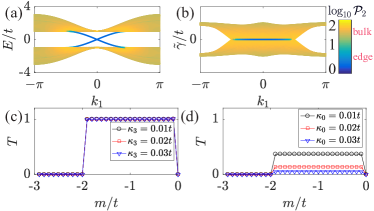
Figure 1: (a) Real part of spectrum $E(k_{1})/t$ of model (2) for $L=40$ and $m=-t$. OBC is applied in the $y$ direction. Colors encode $\log_{10}\mathcal{P}_{2}$. (b) Imaginary part of spectrum $\tilde{\gamma}(k_{1})/t$ for the same parameters used in (a). (c) Transmission coefficient $T$ as a function of $m/t$ for various $\kappa_{3}$. (d) $T$ v.s. $m/t$ with a global loss $-i\kappa_{0}\sigma_{0}$.

To find out $\psi_{\pm}$, we solve the equation $h_{1}(p_{1}=0,-i\partial_{y})\psi_{\pm}=0$ for one specific $m=-t$ and $0<\kappa_{3}\ll t$ and obtain the zero-energy edge states [55]: $\psi_{\pm}=2\sqrt{2}e^{-L/2\pm y}\sinh[(i-\kappa_{3}/t)(y\mp L/2)]\sigma_{2}\phi_{\mp}$. Here, $\psi_{\pm}$ are localized at $y=\pm L/2$, and $\sigma_{1}\phi_{\pm}=\pm\phi_{\pm}$. The effective Hamiltonian of chiral edge states can be obtained by projecting Hamiltonian $h_{1}(p_{1},-i\partial_{y})$ into the space spanned by zero-energy edge states $\psi_{\pm}$, i.e., $[h^{\text{s}}_{1}]_{\alpha\beta}=\langle\psi_{\alpha}|h_{1}(p_{1},-i\partial_{y})|\psi_{\beta}\rangle$ with $\alpha,\beta=\pm$ [51, 52, 53, 55]:

$$\begin{gathered}h^{\text{s}}_{1}(p_{1})=tp_{1}\sigma_{3}+O(p^{2}_{1}).\end{gathered}$$ (3)

Clearly, chiral edge states of Eq. (2) with $m=-t$ are Hermitian. The non-Hermitian parameter $\kappa_{3}$ is encoded in $\psi_{\pm}$ and does not break the Hermicity of chiral edge states.

To verify the Hermicity of chiral edge states of Eq. (2), we compute its energy spectra $\epsilon(k_{1})=E+i\tilde{\gamma}$ of a semi-infinite strip of width $L=40$ through Kwant package [56] and Scipy library [57] and plot $\epsilon(k_{1})$ in Figs. 1(a,b). Colors in Figs. 1(a,b) encode the common logarithmic of participation ratios $\mathcal{P}_{2}$ of a right eigenstate $\psi_{\epsilon}$, defined as $\mathcal{P}_{2}(\epsilon)=\langle(\sum_{\bm{i}}|\psi_{\epsilon}(\bm{i})|^{4})^{-1}\rangle$, where $\psi_{\epsilon}(\bm{i})$ is the wave function amplitude at site $\bm{i}$. $\psi_{\epsilon}$ satisfies $h|\psi(\epsilon)\rangle=\epsilon|\psi(\epsilon)\rangle$ and $\langle\psi_{\epsilon}|\psi_{\epsilon}\rangle=1$. $\mathcal{P}_{2}$ measures how many sites a state occupy from which one can easily identify bulk and edge states [58]. As shown in Figs. 1(a,b), chiral edge states (the blue) of model (2) are Hermitian with $\tilde{\gamma}=0$, while bulk states (the yellow) are non-Hermitian.

Noticeably, Eq. (3) fails for a narrow width, say $L\sim\xi$, where edge states on opposite sites couple each other and open a gap in the complex energy plane [52]. In this case, chiral edge states are non-Hermitian. Besides, we find $|E(p_{1}=0)|$ and $|\tilde{\gamma}(p_{1}=0)|$ decay in an exponentially law of $L/\xi$. In this work, we only focus on the large size limit $L\gg\xi$ where Hermitian chiral edge states are allowed.

While quantized transport in the quantum Hall effect is one of the fundamental properties of Hermitian CIs, previous works show that Hall conductances of non-Hermitian CIs are non-quantized [47, 48, 49, 50]. The reason for the absence of quantized Hall conductances is that edge states of those CIs are non-Hermitian with certain degrees of loss. Naturally, for the Hermitian edge states predicted here, we expect perfectly quantized transport. To see it, we apply Eq. (2) to a Hall bar of size $L\times L$ with two semi-infinite Hermitian leads at two ends along the $x$ direction and compute the transmission coefficient $T(\epsilon)$ by using Büttiker’s approach combined with the non-equilibrium Green function method, where a virtual lead of zero net particle flow is introduced to model the incoherent scatterings [59].

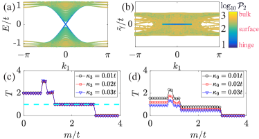
Figure 2: (a) $E(k_{1})/t$ of the non-Hermitian CI for $L=12$, $m=2t$, and $b=0.2t$. (b) $\tilde{\gamma}(k_{1})/t$ for the same parameters of (a). Colors encode $\log_{10}\mathcal{P}_{2}$. (c) $T(0.02t)$ as a function of $m/t$ for various $\kappa_{3}$. (d) $T(0.02t)$ v.s. $m/t$ for a global loss $-i\kappa_{0}\Gamma_{0}$. The cyan line locates $T=1$.

Figure 1(c) displays some representative results with $\epsilon=0.02t$, $L=50$, and various $\kappa_{3}$. Here, $T(0.02t)$ is exactly quantized at 1 for $-2<m/t<0$, irrelevant to the values of $\kappa_{3}$. For a comparison, we also plot $T(0.02t)$ for a different non-Hermitian CI, whose Hermitian part is the same as that of Eq. (2) but the non-Hermicity is a global loss of $-i\kappa_{0}\sigma_{0}$ ($\kappa_{0}>0$), see Fig. 1(d), where chiral edge states are non-Hermitian, and the transmission coefficient is non-quantized, qualitatively consistent with previous studies [47, 48, 49, 50].

3DSOTI.$-$The second example is a non-Hermitian 3DSOTI in a cubic lattice of $a=1$, which belongs to class A [60],

$$\begin{gathered}h_{2}(\bm{k})=t\sum_{\mu=1,2,3}\sin k_{\mu}\Gamma_{\mu}+\left(m-t\sum_{\mu=1,2,3}\cos k_{\mu}\right)\Gamma_{4}\\ +(b+i\kappa_{3})\Gamma_{13}.\end{gathered}$$ (4)

Here, $\Gamma_{\mu=0,1,2,3,4,5}=(\sigma_{0}\otimes\sigma_{0},\sigma_{3}\otimes\sigma_{1},\sigma_{0}\otimes\sigma_{3},\sigma_{1}\otimes\sigma_{1},\sigma_{2}\otimes\sigma_{1},\sigma_{0}\otimes\sigma_{2})$ are the four-by-four identity and one particular choice of gamma matrices that satisfy $\{\Gamma_{\mu},\Gamma_{\nu}\}=2\delta_{\mu,\nu}\Gamma_{0}$ and $\Gamma_{\mu\nu}=[\Gamma_{\mu},\Gamma_{\nu}]/(2i)$. $m$ and $b$ are the masses that control the band inversions of bulk states and surface states, respectively. For $0<b<1$ and $1+b<m<3-b$, the Hermitian part of model (4) is a reflection-symmetric 3DSOTI with the reflection plane of $y=0$. If model (4) is in a cubic lattice of size $L\times\sqrt{2}L\times\sqrt{2}L$ with OBCs on surfaces perpendicular to $(100),(01\bar{1}),(011)$, chiral hinge states will appear at the hinges when two surfaces meet at the reflection plane, e.g., $y=0,z=\pm L$.

We use the same approach in Ref. [61] to derive the effective Hamiltonian of topological surface states of model  (4) by replacing $p_{2}$ by $-i\partial_{y}$ around $\Gamma$ point:

$$\begin{gathered}h^{\text{surface}}_{2}(\bm{p}_{\parallel}=(p_{1},p_{3}))=\begin{bmatrix}h^{+}_{2}(\bm{p}_{\parallel})&0\\ 0&h^{-}_{2}(\bm{p}_{\parallel})\end{bmatrix}\end{gathered}$$ (5)

with $h^{\pm}_{2}(\bm{p}_{\parallel})=\pm[tp_{1}\sigma_{1}+tp_{3}\sigma_{2}-(b+i\kappa_{3}\pm t^{\prime}p^{2}_{\parallel}/2)\sigma_{2}]$, see Supplemental Materials [55]. Here, $m=2t$, and $\sigma_{1,2,3}$ act on the surface states of $\bm{p}_{\parallel}=(0,0)$. $t^{\prime}$ decays exponentially with the distance of two surfaces, while $t^{\prime}=-t/2$ if they meet at the reflection plane of $y=0$.

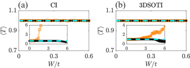
Figure 3: (a) $\langle T(0.02t)\rangle$ as a function of $W/t$ for Hermitian (black stars) and non-Hermitian (orange squares) CIs with $m=-t$ and $L=50$. (b) Same as (a) for Hermitian (black stars) and non-Hermitian (orange squares) 3DSOTIs with $m=2t$, $b=0.2t$, and $L=12$. The cyan lines locate $\langle T(0.02t)\rangle=1$. Insets are for large-disorder regimes.

Equation (5) indicates that the surface Hamiltonian of 3DSOTI act as a non-Hermitian CI with PHS. Band inversion of surface states, as well as the emergence of the hinge states, happens at $h^{+}_{2}(\bm{p}_{\parallel})$ ($h^{-}_{2}(\bm{p}_{\parallel})$) if $b>0$ ($b<0$). Since $h^{\pm}_{2}(\bm{p}_{\parallel})$ does not suffer from the non-Hermitian skin effect, we expect its chiral hinge states are Hermitian.

Figures. 2(a,b) display $E$ and $\tilde{\gamma}$ of Eq. (4) with $L=12$, $m=2t$, $b=0.2t$, and OBCs on $(01\bar{1}),(011)$. We find chiral hinge states appear in the gap of surface states, where $\tilde{\gamma}=0$. Consequently, those chiral hinge states are Hermitian with $T=1$, see Fig. 2(c). While, if we replace $i\kappa_{3}\Gamma_{13}$ by a global loss $-i\kappa_{0}\Gamma_{0}$, the chiral hinge states are non-Hermitian without quantized $T$, see Fig. 2(d).

Equation (4) also supports Hermitian helical hinge states with valley-momentum locking when $0<m<1-b$ [60]. $T$ for Hermitian helical hinge states is quantized (to 2) for $i\kappa_{3}\Gamma_{13}$, irrelevant to the value of $\kappa_{3}$, see Fig. 2(c). However, these hinge states will loss the quantized transport in the presence of disorders due to the facilitation of inter-valley scattering and mixing.

Robustness against disorders.$-$To fully establish these Hermitian edge/hinge states as genuine states of matter, their robustness against disorders should be tested. Here, white-noise on-site random complex potentials, $V_{1}=\sum_{\bm{i}}c^{\dagger}_{\bm{i}}(v^{r}_{\bm{i}}\sigma_{0}+iv^{i}_{\bm{i}}\sigma_{3})c_{\bm{i}}$ and $V_{2}=\sum_{\bm{i}}c^{\dagger}_{\bm{i}}(v^{r}_{\bm{i}}\Gamma_{0}+iv^{i}_{\bm{i}}\Gamma_{31})c_{\bm{i}}$, are added to lattice models of Eqs. (2) and (4), respectively. $c^{\dagger}_{\bm{i}}$ and $c_{\bm{i}}$ are the creation and the annihilation operators on site $\bm{i}$, and $v^{r,i}_{\bm{i}}$ distribute uniformly in $[-W_{r}/2,W_{r}/2]$ and $[-W_{i}/2,W_{i}/2]$, where real numbers $W_{r,i}$ measure the strength of randomness.

Figures 3(a,b) depict the ensemble-averaged $\langle T(W=W_{r}=W_{i})\rangle$ for disordered non-Hermitian CIs ($m=t$) and 3DSOTIs ($m=2t$ and $b=0.2t$) of $\epsilon=0.02t$, respectively. For a comparison, $\langle T\rangle$ for their Hermitian counterparts ($\kappa_{3}=W_{i}=0$) are also computed. Evidently, quantized plateaus of $\langle T\rangle$ persist until a finite disorder $W_{c}$ (depends on model parameters) for both non-Hermitian CI and 3DSOTI. Such plateaus are size-independent (not shown here) with extremely small fluctuations of $T$, which should be convincing supports of the robustness of Hermitian chiral edge/hinge states. However, such chiral edge/hinge states loss their Hermicity if disorders lead to an effective gain/loss, see Supplemental Materials [55].

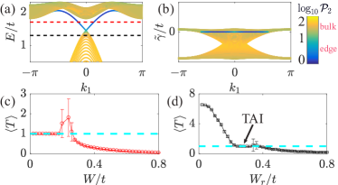
Figure 4: (a,b) Real (a) and imaginary (b) parts of spectrum $\epsilon(k_{1})$ of model (6). Colors encode $\log_{10}\mathcal{P}_{2}$. The dash lines in (a) denote the Fermi energies for $\langle T\rangle$ in (c,d). (c,d) $\langle T\rangle$ v.s. $W/t$ and $W_{r}/t$ for $E=1.3t$ (c) and $E=1.5t$ (d). Here, $m=1.8t$, $t_{0}=-0.8t$, $\kappa_{3}=0.01t$, $\kappa_{0}=-1.2\kappa_{3}$, and $L=100$. The cyan lines denote $\langle T\rangle=1$.

Interestingly, Hermitian and non-Hermitian systems have qualitatively different transport behaviors for $W>W_{c}$. In Hermitian systems, $\langle T\rangle<1$ for $W>W_{c}$ where backward scatterings lead to a non-zero reflection probability; while in non-Hermitian systems, $\langle T\rangle$ could be larger than 1 since the transmission amplitude can be amplified by the non-Hermicity.

TAIs.$-$Saliently, one can also construct Hermitian edge states without PHS, where a global loss/gain is required. This can be seen by introducing a new term $t_{0}\sum_{\mu=1,2}\cos k_{\mu}\sigma_{0}$, which breaks PHS, as well as a compensated loss/gain $i\kappa_{0}\sigma_{0}$ in the non-Hermitian CI [Eq. (2)]:

$$\begin{gathered}h_{3}(\bm{k})=h_{1}(\bm{k})+\left(t_{0}\sum_{\mu=1,2}\cos k_{\mu}+i\kappa_{0}\right)\sigma_{0}.\end{gathered}$$ (6)

Equation (6) belongs to class A. Near $p_{1}=0$, the effective Hamiltonian for chiral edge states reads (to the order of $p_{1}$, and $\kappa_{0},\kappa_{3}\ll t$) [52, 55]

$$\begin{gathered}h^{\text{s}}_{3}(p_{1})=[-mt_{0}/t+i(\kappa_{0}-t_{0}\kappa_{3}/t)]\sigma_{0}+\sqrt{t^{2}-t^{2}_{0}}p_{1}\sigma_{3}.\end{gathered}$$ (7)

Hence, chiral edge states are Hermitian when $\kappa_{0}=t_{0}\kappa_{3}/t$ and $|t_{0}|<|t|$, confirmed in the energy spectrum shown in Figs. 4(a,b) for $m=1.8t$, $t_{0}=-0.8t$, $\kappa_{3}=0.01t$, and $\kappa_{0}=-0.8\kappa_{3}$. Such chiral edge states are robust against the random potentials $V_{1}$ until $W_{c}=0.25t$, supported by the quantized ensemble-average transmission coefficient $\langle T(1.5t)\rangle$ in Fig. 4(c).

In Hermitian systems, TAI, a disorder-induced topological insulator, could emerge in disordered PHS-broken CIs, i.e., the Hermitian part of Eq. (6) subject to the random potential $V_{1}$ with $W_{i}=0$ [62, 63]. TAIs are featured by quantized transmission coefficients at finite disorders when it is topological trivial in crystals. Naturally, one may ask whether there is a non-Hermitian TAI characterized by quantized transport only at finite disorders. Numerical evidence to the existence of non-Hermitian TAIs is shown in Fig. 4(d): There is a plateau of $\langle T(1.3t)\rangle=1$ at finite disorders $W_{r}/t\in[0.25,0.3]$ and $W_{i}=0$, when the system is a topologically-trivial metal at weak disorders $W_{r}/t\in[0,0.25]$ and becomes a topologically-trivial insulator at strong disorders $W_{r}>0.3t$.

Discussions.$-$Hermitian chiral boundary states in non-Hermitian topological insulators reported here are different from real spectra in non-Hermitian systems with PT-symmetry [44, 45, 46]. There exist exceptional points in PT-symmetric systems that separate real spectra in PT-symmetry preserved region from complex spectra in PT-symmetry broken region. Such exceptional points do not occur in the Hermitian chiral boundary states. Hermicity of the boundary states is insensitive to smooth changes of material parameters and cannot be destroyed unless the system undergoes topological phase transitions.

Electronic CIs and 3DSOTIs have been predicted and experimentally observed in many materials such as HgTe [12, 13] and Bi_2-xSm_xSe₃ [64]. However, it is difficult to satisfy the condition of $\kappa_{0}=t_{0}\kappa_{3}/t$ even one can manipulate lifetimes of electrons in different bands, thus $i(\kappa_{0}\sigma_{0}+\kappa_{3}\sigma_{3})$ in CIs. In contrast, recent progress in cold-atom, photonic, and optomechanical systems [65, 66, 67] allows us to control the gain and loss of excitation states in those systems. For example, a topological insulator laser can possess Hermitian chiral edge states in two dimensions, see Supplemental Materials [55].

Conclusion.$-$In conclusion, we showed that it is possible to make the chiral edge/hinge states of non-Hermitian topological insulator passive without gain/loss and immune to non-Hermitian skin effect. Consequently, these chiral edge/hinge states become Hermitian and give rise to quantized edge/hinge transport in non-Hermitian topological insulators. Remarkably, their Hermicity does not rely on any symmetry, e.g., one can have Hermitian chiral edge/hinge states in both class D [respect to particle-hole symmetry] and class A [without symmetry] in AZ symmetry classification.

I Supplemental Materials: Hermitian chiral boundary states in non-Hermitian topological insulators

These Supplemental Materials contain the following information: (S1) Derivations of Eqs. (3,5,7) in the main text. (S2) Disorder effects on the Hermicity of chiral edge states. (S3) Coupled lasers in a honeycomb lattice display the predicted Hermitian chiral edge states.

S1: Derivations of Eqs. (3,5,7) in the main text

In this section, we show how to derive Eqs. (3,5,7) in the main text.

Equation (3): Chern insulators.

Near the $\Gamma$ point ($\bm{k}=(0,0)$), the low-energy effective Hamiltonian of the non-Hermitian Chern insulator (CI) reads

$$\begin{gathered}h_{1}(\bm{p})=tp_{1}\sigma_{1}+tp_{2}\sigma_{2}+\left(\tilde{m}+i\kappa_{3}-\dfrac{t}{2}p^{2}_{1}-\dfrac{t}{2}p^{2}_{2}\right)\sigma_{3}.\end{gathered}$$ (8)

with $\tilde{m}=m+2t$. For one specific parameter of $m=-t$ and $0<\kappa_{3}\ll t$, we have

$$\begin{gathered}h_{1}(\bm{p})=t\left[p_{1}\sigma_{1}+p_{2}\sigma_{2}+\left(1+i\tilde{\kappa}_{3}-\dfrac{1}{2}p^{2}_{1}-\dfrac{1}{2}p^{2}_{2}\right)\sigma_{3}\right]\end{gathered}$$ (9)

with $\tilde{\kappa}_{3}=\kappa_{3}/t$. Periodic boundary condition (PBC) is applied in the $x$-direction, and open boundary condition (OBC) is applied in the $y$-direction such that $p_{2}\to-i\partial_{y}$ and $-L/2<y<L/2$. We split Eq. (9) into two parts:

$$\begin{gathered}h^{1}_{1}(-i\partial_{y})=t\left[-i\partial_{y}\sigma_{2}+\left(1+i\tilde{\kappa}_{3}+\dfrac{1}{2}\partial_{yy}\right)\sigma_{3}\right]\end{gathered}$$ (10)

and

$$\begin{gathered}h^{2}_{1}(p_{1})=t\left(p_{1}\sigma_{1}-\dfrac{1}{2}p^{2}_{1}\sigma_{3}\right).\end{gathered}$$ (11)

Due to particle-hole symmetry, eigenenergies of $h_{1}(p_{1},-i\partial_{y})$ come in pairs of $\{\epsilon(p_{1}),-\epsilon(-p_{1})\}$. To find special edge state wavefunction $\psi(p_{1}=0,y)\equiv\psi(y)$ of $\epsilon=0$, we solve $h^{1}_{1}(-i\partial_{y})\psi=0$ for solution of form $\psi(y)=i\sigma_{2}\phi e^{\lambda_{y}}$:

$$\begin{gathered}t\left[\lambda\phi+\left(1+i\tilde{\kappa}_{3}+\dfrac{\lambda^{2}}{2}\right)\sigma_{1}\phi\right]=0.\end{gathered}$$ (12)

$\phi$ should be the eigenvectors of $\sigma_{1}$, say $\sigma_{1}\phi_{\pm}=\pm\phi$. For $\phi_{+}$, $\lambda$ satisfies

$$\begin{gathered}\lambda+\left(1+i\tilde{\kappa}_{3}+\dfrac{\lambda^{2}}{2}\right)=0\to\lambda_{1,2}=-1\pm\left(i-\tilde{\kappa}_{3}\right).\end{gathered}$$ (13)

For $\phi_{-}$, $\lambda$ is given by

$$\begin{gathered}\lambda-\left(1+i\tilde{\kappa}_{3}+\dfrac{\lambda^{2}}{2}\right)=0\to\lambda_{3,4}=1\pm(i-\tilde{\kappa}_{3}).\end{gathered}$$ (14)

Hence,

$$\begin{gathered}\psi(y)=i\sigma_{2}\left[\left(c_{1}e^{\lambda_{1}y}+c_{2}e^{\lambda_{2}y}\right)\phi_{+}+\left(d_{1}e^{\lambda_{3}y}+d_{2}e^{\lambda_{4}y}\right)\phi_{-}\right]\end{gathered}$$ (15)

with $\text{Re}[\lambda_{3,4}]=-\text{Re}[\lambda_{1,2}]>0$. For edge states localized at $y=-L/2$, we requires $d_{1}=d_{2}=0$ and $\psi(y=-L/2)=0$. Therefore, the solution of edge states localized at $y=-L/2$ reads

$$\begin{gathered}\psi_{-}(y)=i2ce^{-L/2-y}\sinh\left[(i-\tilde{\kappa}_{3})(L/2+y)\right]\sigma_{2}\phi_{+}\end{gathered}$$ (16)

with $c$ being a normalized constant. To normalize $\psi_{-}(y)$ yields $|c|^{2}=2$ if $\tilde{\kappa}_{3}\ll 1$ and $L\gg 1$, and we choose $c=-i\sqrt{2}$ such that

$$\begin{gathered}\psi_{-}(y)=2\sqrt{2}e^{-L/2-y}\sinh\left[(i-\tilde{\kappa}_{3})(L/2+y)\right]\sigma_{2}\phi_{+}.\end{gathered}$$ (17)

Following the same approach, we find the edge states localized on the other side $y=L/2$,

$$\begin{gathered}\psi_{+}(y)=2\sqrt{2}e^{-L/2+y}\sinh[(i-\tilde{\kappa}_{3})(y-L/2)]\sigma_{2}\phi_{-}.\end{gathered}$$ (18)

The effective Hamiltonian for the zero-energy chiral edge states is obtained by projecting bulk Hamiltonian Eq. (10) onto space spanned by $\psi_{\pm}$, i.e., $[h^{s}_{1}]_{\alpha\beta}=\langle\psi_{\alpha}|h_{1}(p_{1},-i\partial_{y})|\psi_{\beta}\rangle$ with $\alpha,\beta=\pm$ [1]. Following this approach, we obtain $h^{s}_{1}=tp_{1}\sigma_{3}+O(p^{2}_{1})$, which is Eq. (3) in the main text.

Equation (5): Three-dimensional second-order topological insulators.

Let us expand Eq. (4) in the main text near the Gamma point, say $\bm{k}=(0,0,0)+\bm{p}$ with $\bm{p}\ll 1$:

$$\begin{gathered}h_{2}(\bm{p})=tp_{1}\Gamma_{1}+tp_{2}\Gamma_{2}+tp_{3}\Gamma_{3}\\ +\left[\tilde{m}+\dfrac{t}{2}\left(p^{2}_{1}+p^{2}_{2}+p^{2}_{3}\right)\right]\Gamma_{4}+(b+i\kappa_{3})\Gamma_{31}\end{gathered}$$ (19)

with $\tilde{m}=m-3t$. Then, we apply the OBC in the $y$ direction, i.e., $p_{2}\to-i\partial_{y}$ and $-L/2<y<L/2$, and divide Eq. (19) into two parts:

$$\begin{gathered}h^{1}_{2}(-i\partial_{y})=-it\partial_{y}\Gamma_{2}+\left(\tilde{m}-\dfrac{t}{2}\partial_{yy}\right)\Gamma_{4}\end{gathered}$$ (20)

and

$$\begin{gathered}h^{2}_{2}(\bm{p}_{\parallel}=(p_{1},p_{3}))=tp_{1}\Gamma_{1}+tp_{3}\Gamma_{3}+\dfrac{t}{2}\left(p^{2}_{1}+p^{2}_{3}\right)\Gamma_{4}\\ +(b+i\kappa_{3})\Gamma_{31}.\end{gathered}$$ (21)

We expect a zero-energy solution of Eq. (20): $h^{1}_{2}(-i\partial_{y})\psi=0$. To obtain $\psi$, we apply a unitary transformation $\tilde{h}_{2}(\bm{p}_{\parallel},-i\partial_{y})=Uh_{2}(\bm{p}_{\parallel},-i\partial_{y})U^{-1}$ with $U=\exp[i\pi\sigma_{1}/4]\otimes\exp[-i\pi\sigma_{1}/4]$. Then, we solve $\tilde{h}^{1}_{2}(-i\partial_{y})\tilde{\psi}=0$ where

$$\begin{gathered}\tilde{h}^{1}_{2}(-i\partial_{y})=\begin{bmatrix}0&t\partial_{y}+\tilde{m}-t\partial_{yy}/2&0&0\\ -t\partial_{y}+\tilde{m}-t\partial_{yy}/2&0&0&0\\ 0&0&0&t\partial_{y}-\tilde{m}+t\partial_{yy}/2\\ 0&0&-t\partial_{y}-\tilde{m}+t\partial_{yy}/2&0\end{bmatrix}\end{gathered}$$ (22)

and $\tilde{\psi}=U\psi$. Consider a specific value $m=2t$. It is clear that $\tilde{\psi}$ have four solutions:

$$\tilde{\psi}_{1}=\tilde{\phi}_{1}\begin{bmatrix}1\\ 0\\ 0\\ 0\end{bmatrix},\tilde{\psi}_{2}=\tilde{\phi}_{2}\begin{bmatrix}0\\ 1\\ 0\\ 0\end{bmatrix},\tilde{\psi}_{3}=\tilde{\phi}_{3}\begin{bmatrix}0\\ 0\\ 1\\ 0\end{bmatrix},\tilde{\psi}_{4}=\tilde{\phi}_{4}\begin{bmatrix}0\\ 0\\ 0\\ 1\end{bmatrix}.$$

Use the trial solution $\tilde{\phi}_{1,2,3,4}=e^{\lambda_{1,2,3,4}y}$. $\lambda_{1}$ satisfies the quadratic equation $\left(-t\partial_{y}-t-t\partial_{yy}/2\right)e^{\lambda_{1}y}=0$. We find $\lambda_{1}=-1\pm i$ such that $\tilde{\phi}_{1}$ localizes at $y=-L/2$. From boundary condition $\tilde{\phi}_{1}(y=-L/2)=0$, we find $\tilde{\phi}_{1}(y)=i2ce^{-y}\sin[y+L/2]$ with $c$ being a normalized constant. Normalization condition gives $|c|^{2}=(2e^{-L})/[1+e^{-2L}(\cos[2L]-\sin[2L]-2)]$, and we choose $c=(-i\sqrt{2}e^{-L/2})/([1+e^{-2L}(\cos[2L]-\sin[2L]-2)]^{1/2})$. Then we have

$$\begin{gathered}\tilde{\phi}_{1}(y)=\dfrac{2\sqrt{2}e^{-(y+L/2)}\sin[y+L/2]}{[1+e^{-2L}(\cos[2L]-\sin[2L]-2)]^{1/2}}.\end{gathered}$$ (23)

Likewise, we obtain

$$\begin{gathered}\tilde{\phi}_{2}(y)=\dfrac{2\sqrt{2}e^{y-L/2}\sin[y-L/2]}{[1+e^{-2L}(\cos[2L]-\sin[2L]-2)]^{1/2}},\end{gathered}$$ (24)

and

$$\begin{gathered}\tilde{\phi}_{3}(y)=\tilde{\phi}_{2}(y),~{}\tilde{\phi}_{4}(y)=\tilde{\phi}_{1}(y).\end{gathered}$$ (25)

The surface Hamiltonian can be obtained by projecting the bulk Hamiltonian into the space spanned by the four specific surface states [61]

$$\begin{gathered}h^{\text{surface}}_{2}(\bm{p}_{\parallel})=\int\begin{bmatrix}\tilde{\psi}^{\dagger}_{1}\\ \tilde{\psi}^{\dagger}_{2}\\ \tilde{\psi}^{\dagger}_{3}\\ \tilde{\psi}^{\dagger}_{4}\\ \end{bmatrix}\left(Uh_{2}(\bm{p}_{\parallel},-i\partial_{y})U^{-1}\right)\begin{bmatrix}\tilde{\psi}_{1}&\tilde{\psi}_{2}&\tilde{\psi}_{3}&\tilde{\psi}_{4}\end{bmatrix}dy\\ =tp_{1}\sigma_{1}\otimes\sigma_{1}+tp_{3}\sigma_{2}\otimes\sigma_{1}-(b+i\kappa_{3})\sigma_{3}\otimes\sigma_{0}\\ -\dfrac{t^{\prime}}{2}(p^{2}_{1}+p^{2}_{3})\sigma_{3}\otimes\sigma_{1}.\end{gathered}$$ (26)

Again, we perform a unitary transformation $U^{\prime}=\sigma_{0}\otimes\exp[-\pi\sigma_{3}/4]$ to Eq. (26) and write the effective Hamiltonian for the surface states in the following form:

$$\begin{gathered}h^{\text{surf}}_{2}=\begin{bmatrix}h^{+}_{2}(\bm{p}_{\parallel})&0\\ 0&h^{-}_{2}(\bm{p}_{\parallel})\end{bmatrix}\end{gathered}$$ (27)

with $h^{\pm}_{2}(\bm{p}_{\parallel})=\pm[tp_{1}\sigma_{1}+tp_{3}\sigma_{2}-(b+i\kappa_{3}\pm t^{\prime}(p^{2}_{1}+p^{2}_{3})/2)\sigma_{3}]$. Equation (27) is Eq. (5) in the main text. Here, we introduce a new quantity $t^{\prime}$:

$$\begin{gathered}t^{\prime}=t\int^{L/2}_{-L/2}\tilde{\phi}^{\ast}_{1}(y)\tilde{\phi}_{2}(y)dy=t\dfrac{4e^{-L}(L\cos[L]-\sin[L])}{[1+e^{-2L}(\cos[2L]-\sin[2L]-2)]}\end{gathered}$$ (28)

Equation (28) vanishes for $L\gg 1$ since $t^{\prime}$ decreases exponentially with $L$. On the other hand, at the hinges where two surfaces meet $L\ll 1$, $t^{\prime}=-t/2$.

Equation (7): Topological Anderson insulators.

We expand Eq. (7) in the main text near the $\Gamma$ point to obtain the low-energy effective Hamiltonian:

$$\begin{gathered}h_{3}(\bm{p})=tp_{1}\sigma_{1}+tp_{2}\sigma_{2}+\left[\tilde{m}+i\kappa_{3}-\dfrac{t}{2}\left(p^{2}_{1}+p^{2}_{2}\right)\right]\sigma_{3}\\ +\left[2t_{0}+i\kappa_{0}-\dfrac{t_{0}}{2}\left(p^{2}_{1}+p^{2}_{2}\right)\right]\sigma_{0}\end{gathered}$$ (29)

with $\tilde{m}=m+2t$. We now solve the eigenfunction of the following Hamiltonian:

$$\begin{gathered}\tilde{h}_{3}(\bm{p})=h_{3}(\bm{p})-\left(2t_{0}+i\kappa_{0}\right)\sigma_{0}=tp_{1}\sigma_{1}+tp_{2}\sigma_{2}\\ +\left[\tilde{m}+i\kappa_{3}-\dfrac{t}{2}\left(p^{2}_{1}+p^{2}_{2}\right)\right]\sigma_{3}-\dfrac{t_{0}}{2}\left(p^{2}_{1}+p^{2}_{2}\right)\sigma_{0}\end{gathered}$$ (30)

in a finite strip of a width $L$ with the PBC applied in the $x$ direction and the OBC applied in the $y$ direction. Now, $p_{1}$ is still a good quantum number, and $p_{2}=-i\partial_{y}$, i.e.,

$$\begin{gathered}\left\{\begin{array}[]{c}\left[\tilde{m}+i\kappa_{3}-b_{+}(p^{2}_{1}-\partial_{yy})\right]\psi_{1}+t(p_{1}-\partial_{y})\psi_{2}=\epsilon\psi_{1}\\ \\ t(p_{1}+\partial_{y})\psi_{1}-\left[\tilde{m}+i\kappa_{3}-b_{-}\left(p^{2}_{1}-\partial_{yy}\right)\right]\psi_{2}=\epsilon\psi_{2}\end{array}\right.\end{gathered}$$ (31)

with $b_{+}=(t+t_{0})/2$ and $b_{-}=(t-t_{0})/2$. From Eq. (31), one can find the energy spectrum $\epsilon$ for $L\gg 1$ near $p_{1}=0$ by using the trial function $\psi_{1,2}=e^{\lambda y}$ [The details are illustrated in Ref. [52]]:

$$\begin{gathered}\epsilon_{\pm}(p_{1})=-\dfrac{t_{0}}{t}\left(\tilde{m}+i\kappa_{3}\right)\pm\sqrt{t^{2}-t^{2}_{0}}p_{1}\end{gathered}$$ (32)

providing $t^{2}>t^{2}_{0}$. Recall that $\epsilon_{\pm}(p_{1})$ are the dispersions for Eq. (30), but not that of Eq. (29), where a constant complex energy $\left(2t_{0}+i\kappa_{0}\right)$ is shifted. Hence, the edge state spectrum of the original Hamiltonian $h_{3}(\bm{p})$ should be

$$\begin{gathered}\epsilon_{\pm}(p_{1})=\left[-t_{0}m/t+i(\kappa_{0}-t_{0}\kappa_{3}/t)\right]\pm\sqrt{t^{2}-t^{2}_{0}}p_{1}\end{gathered}$$ (33)

We use the same approach for obtaining the effective Hamiltonian of chiral edge states of the non-Hermitian CI: $[h^{s}_{3}]_{\alpha\beta}=\langle\psi_{\alpha}|h_{3}(p_{1},-i\partial_{y})|\psi_{\beta}\rangle$ with $\alpha,\beta=\pm$ and $h_{3}(p_{1},-i\partial_{y})|\psi_{\alpha}\rangle=\epsilon_{\alpha}(p_{1})|\psi_{\alpha}\rangle$:

$$\begin{gathered}h^{s}_{3}(p_{1})=\left[-t_{0}m/t+i(\kappa_{0}-t_{0}\kappa_{3}/t)\right]\sigma_{0}+\sqrt{t^{2}-t^{2}_{0}}p_{1}\sigma_{3}.\end{gathered}$$ (34)

Equation (34) is Eq. (7) in the main text.

S2: Disorder effects on the Hermicity of chiral edge states

The keys for realizing Hermitian chiral edge states are: (i) chiral edge states have no gain and no loss; (ii) the chiral edge states can propagate along sample boundaries without suffering from the non-Hermitian skin effect [Otherwise, they become corner states]. Therefore, any disorders that lead to the gain/loss or the non-Hermitian skin effect on chiral edge states break their Hermicity. Within a simple self-consistent Born approximation, the effective Hamiltonian of a disordered system is $h_{\text{eff}}(\bm{k})=h_{0}(\bm{k})+\Sigma$ with $h_{0}(\bm{k})$ being the Hamiltonian of a clean system and $\Sigma$ being the disorder-induced self-energy. In the continuous limit, the self-energy in the first-order reads [4]

$$\begin{gathered}\Sigma^{1}=\dfrac{1}{V}\int U(\bm{x})d^{d}x=\langle U(\bm{x})\rangle.\end{gathered}$$ (35)

Here, $U(\bm{x})$ describes the profile of random potentials, and $V$ is the volume of the system. Hence, the first-order self-energy shifts the complex-energy spectrum by a constant proportional to the disordered potential’s spatial average. In the main text where $\langle U(\bm{x})\rangle=0,\langle U^{2}(\bm{x})\rangle=W^{2}/12$, this average is zero. Thus, disorders do not lead to gain/loss for chiral boundary states. However, for disorders that is $\langle U(\bm{x})\rangle=i\kappa$, a global gain ($\kappa>0$) or loss ($\kappa<0$) arise from the disorders. The Hermicity of the chiral edge states is lost.

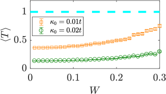
Figure 5: Ensemble-averaged transmission coefficient $\langle T(0.02t)\rangle$ as a function of disorder $W$ for $\kappa=0.01,0.02$ for non-Hermitian Chern insulators [Parameters are the same as those for Fig. 3 in the main text]. The cyan line locate $\langle T(0.02t)\rangle=1$.

To illustrate the above point, we consider the following disorders

$$\begin{gathered}V_{\text{broken}}=\sum_{\bm{i}}c^{\dagger}_{\bm{i}}\left(i\tilde{v}^{i}_{\bm{i}}\sigma_{0}\right)c_{\bm{i}}\end{gathered}$$ (36)

with $\tilde{v}^{i}_{\bm{i}}$ distributing uniformly in $[\kappa-W/2,\kappa+W/2]$ to the lattice model of the non-Hermitian Chern insulator $h_{1}(\bm{k})$ and calculate the transmission coefficient $T$ as a function of $W$ (in the unit of hopping energy $t$) for the same parameters as those for Fig. 3 in the main text. The results are shown in Fig. 5. Since a global loss is effectively introduced through the disorders, chiral edge states become non-Hermitian such that $\langle T\rangle<1$.

S3: Topological Hermitian laser mode in a laser cavity network

Experimentally [5] and theoretically [6], it is shown that a laser cavity network possesses topologically protected chiral boundary modes in the presence of non-Hermicity. We consider a Haldane design of the laser network where the laser resonators are arranged in a honeycomb lattice. Each resonator is coupled to its nearest-neighbours with a real coupling constant $t_{1}$ and to its next-nearest-neighbours with a complex coupling constant $t_{2}\exp[i\phi]$, where $\phi$ is the Haldane flux parameter [6]. The dynamics of the laser field reads

$$\begin{gathered}\left\{\begin{array}[]{c}i\dfrac{\partial a_{\bm{n}}}{\partial t}=\dfrac{\partial H}{\partial a^{\ast}_{\bm{n}}}=\omega_{0}a_{\bm{n}}+t_{1}\sum_{\langle\bm{nm}\rangle}b_{\bm{m}}+t_{2}e^{i\phi}\sum_{\langle\langle\bm{nm}\rangle\rangle}a_{\bm{m}}-i\gamma a_{\bm{n}}+\dfrac{ig_{a}\mathbb{P}}{1+|\Psi|^{2}/I_{\text{sat}}}a_{\bm{n}}\\ \\ i\dfrac{\partial b_{\bm{n}}}{\partial t}=\dfrac{\partial H}{\partial b^{\ast}_{\bm{n}}}=\omega_{0}b_{\bm{n}}+t_{1}\sum_{\langle\bm{nm}\rangle}a_{\bm{m}}+t_{2}e^{-i\phi}\sum_{\langle\langle\bm{nm}\rangle\rangle}b_{\bm{m}}-i\gamma b_{\bm{n}}+\dfrac{ig_{b}\mathbb{P}}{1+|\Psi|^{2}/I_{\text{sat}}}b_{\bm{n}}.\end{array}\right..\end{gathered}$$ (37)

Here, $a_{\bm{n}}$ and $b_{\bm{n}}$ are the laser field amplitudes at a site $\bm{n}=(x_{\bm{n}},y_{\bm{n}})$ of A and B sub-lattices, respectively. $\langle\bm{nm}\rangle$ and $\langle\langle\bm{nm}\rangle\rangle$ denote the nearest-neighbour sites and the next-nearest-neighbor sites, respectively. $\omega_{0}$ is the resonance frequency of the resonator. $\gamma$ represents the linear loss of a resonator. The last terms in Eq. (37) represent optical gains via stimulated emission that is inherently saturated ($I_{\text{sat}}$). $\mathbb{P}$ is the pump profile, and $g_{a,b}$, the gain parameters of sub-lattice $A$ and $B$, depend on the pump intensity that can be tuned. Hereafter, we set

$$\begin{gathered}\tilde{g}_{a,b}=\dfrac{g_{a,b}\mathbb{P}}{1+|\Psi|^{2}/I_{\text{sat}}}.\end{gathered}$$ (38)

From Eq. (37), we derive the effective non-Hermitian Hamiltonian of the topological insulator laser:

$$\begin{gathered}H=\sum_{\bm{n}}\left[\left(-i\gamma+i\tilde{g}_{a}\right)|a_{\bm{n}}|^{2}+\left(-i\gamma+i\tilde{g}_{b}\right)|b_{\bm{n}}|^{2}\right]+H_{\text{Haldane}}.\end{gathered}$$ (39)

$H_{\text{Haldane}}$ is the standard Haldane Hamiltonian [7] that depends on the resonance frequency of a single resonator. In the absence of disorders, $H$ can be block diagonalized in the momentum space

$$\begin{gathered}H=\sum_{\bm{k}}\begin{bmatrix}a^{\ast}_{\bm{k}}&b^{\ast}_{\bm{k}}\end{bmatrix}h(\bm{k})\begin{bmatrix}a_{\bm{k}}\\ b_{\bm{k}}\end{bmatrix},\end{gathered}$$ (40)

where

$$\begin{gathered}h(\bm{k})=h_{0}\sigma_{0}+\bm{h}\cdot\bm{\sigma}\end{gathered}$$ (41)

with

$$\begin{gathered}\left\{\begin{array}[]{ccc}h_{0}&=&2t_{2}\cos\phi\sum_{i=1,2,3}\cos[\bm{k}\cdot\bm{v}_{i}]+i\left[-\gamma+\dfrac{1}{2}(\tilde{g}_{a}+\tilde{g}_{b})\right]\\ \\ h_{1}&=&t_{1}\sum_{i=1,2,3}\cos[\bm{k}\cdot\bm{u}_{i}]\\ \\ h_{2}&=&-t_{1}\sum_{i=1,2,3}\sin[\bm{k}\cdot\bm{u}_{i}]\\ \\ h_{3}&=&2t_{2}\sin\phi\sum_{i=1,2,3}\sin[\bm{k}\cdot\bm{v}_{i}]+i\dfrac{\tilde{g}_{a}-\tilde{g}_{b}}{2}\\ \end{array}\right..\end{gathered}$$ (42)

Here, $\bm{u}_{1}=(\sqrt{3}/2,1/2),\bm{u}_{2}=(-\sqrt{3}/2,1/2),\bm{u}_{3}=-(\bm{u}_{1}+\bm{u}_{2})$, and $\bm{v}_{1}=\bm{u}_{2}-\bm{u}_{3},\bm{v}_{2}=\bm{u}_{3}-\bm{u}_{1},\bm{v}_{3}=\bm{u}_{1}-\bm{u}_{2}$. The Hermitian part of Eq. (41) supports chiral edge states for $t_{2}\neq 0$ and $-\pi<\phi<\pi$. If the global gain/loss is prohibited, say

$$\begin{gathered}\left[-\gamma+\dfrac{1}{2}(\tilde{g}_{a}+\tilde{g}_{b})\right]=0,\end{gathered}$$ (43)

the chiral edge states are Hermitian.

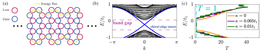
Figure 6: (a) Geometry of a topological laser based on the Haldane design: A honeycomb lattice of coupled microring resonators with armchair edge in the $y$-direction. The output couplers (not shown here) are attached at the $x$-direction. A topological laser mode with unidirectional energy flux (yellow arrows) appears at boundaries. (b) Band spectrum of a passive (neither gain nor loss) topological insulator laser of the geometry shown in (a) [we have applied periodic boundary condition in the $x-$direction]. Here, $t_{2}=0.1t_{1},\phi=\pi/5,\kappa=0$. (c) Quasi-particle energy $E$ (real part) v.s. transmission coefficient $T$ of laser modes in the presence of gain and loss given by Eq. (44) for $\kappa=0.005t_{1},0.01t_{1}$. As a comparison, those of the passive topological insulator laser are also plotted. Cyan dash line locates $T=1$.

To confirm above results, we choose

$$\begin{gathered}\tilde{g}_{a}=\gamma+\kappa,\tilde{g}_{b}=\gamma-\kappa\end{gathered}$$ (44)

with $\kappa$ being a real positive number such that Eq. (43) is satisfied. We specifically design the honeycomb lattice to be an armchair ribbon in the $y$-direction as shown in Fig. 6(a). In the topological phase, e.g., $t_{2}=0.1t_{1},\phi=\pi/5$, spectrum of this armchair strip has a band gap with topologically protected chiral edge states winding around the boundary, see the band spectrum of a passive case (no gain and loss) shown in Fig. 6(b). Once the non-Hermicity is turned on by increasing $\kappa$, the topological band gap does not close, and no topological phase transition occurs. During this process, the bulk states become non-Hermitian, but, importantly, as shown in Fig. 6(c), the chiral edge states remain Hermitian that is characterized by quantized transmission coefficient $T=1$. This means that the edge lasing modes in our design have uniform intensity along the propagating path.

References

[1]
D. J. Thouless, M. Kohmoto, M. P. Nightingale, and M. den Nijs,
Quantized Hall Conductance in a Two-Dimensional Periodic Potential,
Phys. Rev. Lett. 49, 405 (1982).
[2]
F. D. M. Haldane,
Model for a Quantum Hall Effect without Landau Levels: Condensed-Matter Realization of the “Parity Anomaly”,
Phys. Rev. Lett. 61, 2015 (1988).
[3]
X.-G. Wen,
Topological Orders and Edge Excitations in Fractional Quantum Hall States,
Adv. Phys. 44, 405 (1995).
[8]
C.-K. Chiu, J. C. Y. Teo, A. P. Schnyder, and S. Ryu,
Classification of Topological Quantum Matter with Symmetries,
Rev. Mod. Phys. 88, 035005 (2016).
[12]
B. A. Bernevig, T. L. Hughes, and S.-C. Zhang,
Quantum Spin Hall Effect and Topological Phase Transition in HgTe Quantum Wells,
Science 314, 1757 (2006).
[13]
M. König, S. Wiedmann, C. Brüne, A. Roth, H. Buhmann, L. W. Molenkamp, X.-L. Qi, and S.-C. Zhang,
Quantum Spin Hall Insulator State in HgTe Quantum Wells,
Science 318, 766 (2007).
[14]
C.-Z. Chang, J. Zhang, X. Feng, J. Shen, Z. Zhang, M. Guo, K. Li, Y. Ou, P. Wei, L.-L. Wang, et al,
Experimental Observation of the Quantum Anomalous Hall Effect in a Magnetic Topological Insulator,
Science 340, 167 (2013).
[15]
C. L. Kane and T. C. Lubensky,
Topological Boundary Modes in Isostatic Lattices,
Nat. Phys. 10, 39 (2014).
[16]
X. S. Wang, Y. Su, and X. R. Wang,
Topologically protected unidirectional edge spin waves and beam splitter,
Phys. Rev. B 95, 014435 (2017).
[17]
Y. Su, X. S. Wang, and X. R. Wang,
Magnonic Weyl semimetal and chiral anomaly in pyrochlore ferromagnets,
Phys. Rev. B 95, 224403 (2017).
[18]
F. D. M. Haldane and S. Raghu,
Possible Realization of Directional Optical Waveguides in Photonic Crystals with
Broken Time-Reversal Symmetry,
Phys. Rev. Lett. 100, 013904 (2008).
[19]
M. Hafezi, E. A. Demler, M. D. Lukin, and J. M. Taylor,
Robust Optical Delay Lines with Topological Protection,
Nat. Phys. 7, 907 (2011).
[21]
I. Bloch, J. Dalibard, and S. Nascimbéne,
Quantum Simulations with Ultracold Quantum Gases,
Nat. Phys. 8, 267 (2012).
[22]
E. Prodan, T. L. Hughes, and B. A. Bernevig,
Entanglement Spectrum of a Disordered Topological Chern Insulator,
Phys. Rev. Lett. 105, 115501 (2010).
[23]
S. Liu, T. Ohtsuki, and R. Shindou,
Effect of Disorder in a Three-Dimensional Layered Chern Insulator,
Phys. Rev. Lett. 116, 066401 (2016).
[24]
C. Liu, Y. Wang, H. Li, Y. Wu, Y. Li, J. Li, K. He, Y. Xu, J. Zhang, and Y. Wang,
Robust axion insulator and Chern insulator phases in a two-dimensional antiferromagnetic topological insulator,
Nat. Mater. 19 522 (2020).
[25]
N. Hatano and D. R. Nelson,
Localization Transitions in Non-Hermitian Quantum Mechanics,
Phys. Rev. Lett. 77, 570 (1996).
[26]
K. G. Makris, R. El-Ganainy, D. N. Christodoulides, and Z. H. Musslimani,
Beam Dynamics in Symmetric Optical Lattices,
Phys. Rev. Lett. 100, 103904 (2008).
[28]
Y. Xu, S.-T. Wang, and L.-M. Duan,
Weyl Exceptional Rings in a Three-Dimensional Dissipative Cold Atomic Gas,
Phys. Rev. Lett. 118, 045701 (2017).
[29]
F. K. Kunst, E. Edvardsson, J. C. Budich, and E. J. Bergholtz,
Biorthogonal Bulk-Boundary Correspondence in Non-Hermitian Systems,
Phys. Rev. Lett. 121, 026808 (2018).
[31]
L. Zhou and J. Gong,
Non-Hermitian Floquet topological phases with arbitrarily many real-quasienergy edge states,
Phys. Rev. B 98, 205417 (2018).
[32]
Z. Gong, Y. Ashida, K. Kawabata, K. Takasan, S. Higashikawa, and M. Ueda,
Topological Phases of Non-Hermitian Systems,
Phys. Rev. X 8, 031079 (2018).
[34]
K. Kawabata, K. Shiozaki, M. Ueda, and M. Sato,
Symmetry and Topology in Non-Hermitian Physics,
Phys. Rev. X 9, 041015 (2019).
[35]
C. H. Lee, L. Li, and J. Gong,
Hybrid Higher-Order Skin-Topological Modes in Nonreciprocal Systems,
Phys. Rev. Lett. 123, 016805 (2019).
[36]
X. Luo, T. Ohtsuki, and R. Shindou,
Universality Classes of the Anderson Transitions Driven by Non-Hermitian Disorder,
Phys. Rev. Lett. 126, 090402 (2021).
[37]
H. Liu, J.-K. Zhou, B.-L. Wu, Z.-Q. Zhang, H. Jiang,
Real space topological invariant and higher-order topological Anderson insulator in two-dimensional non-Hermitian systems,
Phys. Rev. B 103, 224203 (2021).
[39]
C. Wang and X. R. Wang,
Level statistics of extended states in random non-Hermitian Hamiltonians,
Phys. Rev. B 101, 165114 (2020).
[40]
B. Bahari, A. Ndao, F. Vallini, A. El Amili, Y. Fainman, and B. Kanté,
Nonreciprocal Lasing in Topological Cavities of Arbitrary Geometries,
Science 358, 636 (2017).
[41]
G. Harari, M. A. Bandres, Y. Lumer, M. C. Rechtsman, Y. D. Chong, M. Khajavikhan, D. N. Christodoulides, and M. Segev,
Topological Insulator Laser: Theory,
Science 359, eaar4003 (2018).
[42]
M. A. Bandres, S. Wittek, G. Harari, M. Parto, J. Ren, M. Segev, D. Christodoulides, and M. Khajavikhan,
Topological Insulator Laser: Experiments,
Science 359, eaar4005 (2018).
[43]
K. Kawabata, S. Higashikawa, Z. Gong, Y. Ashida, and M. Ueda,
Topological Unification of Time-Reversal and Particle-Hole Symmetries in Non-Hermitian Physics,
Nat. Commun. 10, 297 (2019).
[44]
C. M. Bender and S. Boettcher,
Real Spectra in Non-Hermitian Hamiltonians Having PT Symmetry,
Phys. Rev. Lett. 80, 5243 (1998).
[45]
H. Yang, C. Wang, T. Yu, Y. Cao, and P. Yan,
Antiferromagnetism Emerging in a Ferromagnet with Gain,
Phys. Rev. Lett. 121, 197201 (2018).
[47]
T. M. Philip, M. R. Hirsbrunner, and M. J. Gilbert,
Loss of Hall conductivity quantization in a non-Hermitian quantum anomalous Hall insulator,
Phys. Rev. B 98, 155430 (2018).
[49]
S. Groenendijk, T. L. Schmidt, and T. Meng,
Universal Hall conductance scaling in non-Hermitian Chern insulators,
Phys. Rev. Research 3, 023001 (2021).
[51]
M. König, H. Buhmann, L. W. Molenkamp, T. L. Hughes, C.-X. Liu, X. L. Qi, and S. C. Zhang,
The Quantum Spin Hall Effect: Theory and Experiment,
J. Phys. Soc. Jpn. 77, 031007 (2008).
[52]
B. Zhou, H.-Z. Lu, R.-L. Chu, S.-Q. Shen, and Q. Niu,
Finite Size Effects on Helical Edge States in a Quantum Spin-Hall System,
Phys. Rev. Lett. 101, 246807 (2008).
[53]
J. Linder, T. Yokoyama, and A. Sudbø,
Anomalous finite size effects on surface states in the topological insulator ,
Phys. Rev. B 80, 205401 (2009).
[54]
X.-L. Qi, Y.-S. Wu, and S.-C. Zhang,
Topological quantization of the spin Hall effect in two-dimensional paramagnetic semiconductors,
Phys. Rev. B 74, 085308 (2006).
[55]
See Supplemental Materials at http://link.aps.org/supplemental.
[56]
C. W. Groth, M. Wimmer, A. R. Akhmerov, and X. Waintal,
Kwant: A software package for quantum transport,
New J. Phys. 16, 063065 (2014).
[57]
P. Virtanen, R. Gommers, T. E. Oliphant, M. Haberland, T. Reddy, D. Cournapeau, E. Burovski, P. Peterson, W. Weckesser,
J. Bright et al.,
SciPy 1.0: fundamental algorithms for scientific computing in Python,
Nat. Methods 17, 261 (2020).
[58]
C. Wang, Y. Su, Y. Avishai, Y. Meir, and X. R. Wang,
Band of Critical States in Anderson Localization in a Strong Magnetic Field with Random Spin-Orbit Scattering,
Phys. Rev. Lett. 114, 096803 (2015).
[59]
S. Datta, Electronic transport in mesoscopic systems (Cambridge university press, 1997).
[60]
C. Wang and X. R. Wang
Disorder-induced quantum phase transitions in three-dimensional second-order topological insulators,
Phys. Rev. Research 2, 033521 (2020).
[61]
C. Wang and X. R. Wang,
Robustness of helical hinge states of weak second-order topological insulators,
Phys. Rev. B 103, 115118 (2021).
[63]
C. W. Groth, M. Wimmer, A. R. Akhmerov, J. Tworzydło, and C. W. J. Beenakker,
Theory of the Topological Anderson Insulator,
Phys. Rev. Lett. 103, 196805 (2009).
[64]
C. Yue, Y. Xu, Z. Song, H Weng, Y.-M. Lu, C. Fang, and X. Dai,
Symmetry-enforced chiral hinge states and surface quantum anomalous Hall effect in the magnetic axion insulator
Bi2-xSmxSe3,
Nat. Phys. 15, 577 (2019).
[65]
G. Barontini, R. Labouvie, F. Stubenrauch, A. Vogler, V. Guarrera, and H. Ott,
Controlling the Dynamics of an Open Many-Body Quantum System with Localized Dissipation,
Phys. Rev. Lett. 110, 035302 (2013).
[66]
H. Xu, D. Mason, L. Jiang, and J. G. E. Harris,
Topological Energy Transfer in an Optomechanical System with Exceptional Points,
Nature (London) 537, 80 (2016).
[67]
W. Chen, Ş. K. Özdemir, G. Zhao, J. Wiersig, and L. Yang,
Exceptional Points Enhance Sensing in an Optical Microcavity,
Nature (London) 548, 192 (2017).

References

[1]
M. König, H. Buhmann, L. W. Molenkamp, T. L. Hughes, C.-X. Liu, X. L. Qi, and S. C. Zhang,
The Quantum Spin Hall Effect: Theory and Experiment,
J. Phys. Soc. Jpn. 77, 031007 (2008).
[2]
C. Wang and X. R. Wang,
Robustness of helical hinge states of weak second-order topological insulators,
Phys. Rev. B 103, 115118 (2021).
[3]
B. Zhou, H.-Z. Lu, R.-L. Chu, S.-Q. Shen, and Q. Niu,
Finite Size Effects on Helical Edge States in a Quantum Spin-Hall System,
Phys. Rev. Lett. 101, 246807 (2008).
[4]
E. Akkermans, and G. Montambaux, Mesoscopic Physics of Electrons and Photons (Cambridge University Press, Cambridge, 2007).
[5]
M. A. Bandres, S. Wittek, G. Harari, M. Parto, J. Ren, M. Segev, D. Christodoulides, and M. Khajavikhan,
Topological Insulator Laser: Experiments,
Science 359, eaar4005 (2018).
[6]
G. Harari, M. A. Bandres, Y. Lumer, M. C. Rechtsman, Y. D. Chong, M. Khajavikhan, D. N. Christodoulides, and M. Segev,
Topological Insulator Laser: Theory,
Science 359, eaar4003 (2018).
[7]
F. D. M. Haldane,
Model for a Quantum Hall Effect without Landau Levels: Condensed-Matter Realization of the “Parity Anomaly”,
Phys. Rev. Lett. 61, 2015 (1988).