Estimating the contribution of foreground halos to the FRB 180924 dispersion measure

Abstract

Fast Radio Burst (FRB) dispersion measures (DMs) record the presence of ionized baryons that are otherwise invisible to other techniques enabling resolution of the matter distribution in the cosmic web. In this work, we aim to estimate the contribution to FRB 180924 DM from foreground galactic halos. Localized by ASKAP to a massive galaxy, this sightline is notable for an estimated cosmic web contribution to the DM (${\rm DM}_{\rm cosmic}$= 220 ${\rm pc\,cm^{-3}}$), which is less than the average value at the host redshift (z = 0.3216) estimated from the Macquart relation (280 ${\rm pc\,cm^{-3}}$). In the favored models of the cosmic web, this suggests few intersections with foreground halos at small impact parameters ($\lesssim 100$ kpc). To test this hypothesis, we carried out spectroscopic observations of the field galaxies within $\sim$1′ of the sightline with VLT/MUSE and Keck/LRIS. Furthermore, we developed a probabilistic methodology that leverages photometric redshifts derived from wide-field DES and WISE imaging. We conclude that there is no galactic halo that closely intersects the sightline and also that the net DM contribution from halos, ${\rm DM}_{\rm halos}$ $<45~{}{\rm pc\,cm^{-3}}$ (95 % c.l.). This value is lower than the ${\rm DM}_{\rm halos}$ estimated from an “average” sightline (121 ${\rm pc\,cm^{-3}}$) using the Planck $\Lambda$CDM model and the Aemulus halo mass function and reasonably explains its low ${\rm DM}_{\rm cosmic}$ value. We conclude that FRB 180924 represents the predicted majority of sightlines in the universe with no proximate foreground galactic halos. Our framework lays the foundation for a comprehensive analysis of FRB fields in the near future.

1 Introduction

Fast Radio Bursts (FRBs) are millisecond-duration, energetic ($\sim 10^{44}$ erg) radio transient events. In recent years, numerous FRBs have been localized and most FRBs are confirmed to be extragalactic (e.g. Lorimer et al., 2007; Bannister et al., 2019; Tendulkar et al., 2017; Law et al., 2020). Although their generation mechanism is yet unknown, FRBs represent a new tool in the repertoire of an observational cosmologist to probe matter and cosmological structure in the universe. Astronomers have used quasar absoprtion lines to study neutral gas in the circumgalactic medium (e.g. Bahcall & Spitzer, 1969; Chen & Tinker, 2008; Prochaska et al., 2011; Tumlinson et al., 2013; Werk et al., 2014; Wilde et al., 2021) for the last several decades. Now, with their unique transient signal, FRBs enable us to capture information about all ionized matter along their lines-of-sight, thus unlocking an opportunity to study previously invisible gas in the universe. One of the measurable properties of FRBs is their dispersion measure (DM), which is the cosmological-scale-factor-weighted line of sight integral of electron density. Even with a handful of localized FRBs, Macquart et al. (2020) were able to show that the observed FRB DMs are consistent with the expected matter distribution in a $\Lambda$CDM universe, thus conclusively resolving the Missing Baryon Problem. While their work “found” the Missing Baryons, the next phase of research is to precisely locate them within the cosmic web. Specifically, we aim to develop the framework to utilize these data and reconstruct the distribution of matter along the sightlines.

Being an integral, one can split the FRB DM into disjoint summative parts corresponding to each “electron reservoir” along the line of sight, namely the host galaxy and its halo; intervening foreground halos and cosmic web filaments; and the Milky Way including its gaseous halo, i.e.

$${\rm DM}_{\rm FRB}={\rm DM}_{\rm host}+{\rm DM}_{\rm cosmic}+{\rm DM}_{\rm MW}$$ (1)

A full characterization of ${\rm DM}_{\rm FRB}$ requires detailed information on the host (e.g. Chittidi et al., 2020) and the intervening cosmic web structures. Simha et al. (2020) performed such an analysis on the sightline of FRB 190608 owing to the favorable location of the FRB in the SDSS spectroscopic footprint. This provided detailed information on the redshifts of foreground galaxies, allowing for a nearly complete characterization of their DM contributions (although with significant uncertainty) and also the contribution from the diffuse intergalactic medium (IGM). In general, if a FRB host is located at low redshifts ($z<0.05$), one could use just the 2MASS Redshift Catalog (Huchra et al., 2012) to perform the same analysis. However, the vast majority of localized FRBs to date fall outside the extant SDSS coverage, and therefore one would require extensive new spectroscopic observations. In this work, we explore the application of photometric redshifts combined with sparse spectroscopy to estimate the DM contributions of foreground halos, ${\rm DM}_{\rm halos}$, for one such sightline: FRB 180924.

FRB 180924 was the first apparently non-repeating FRB to be discovered and localized by the Australian Square-Kilometer Array Pathfinder (ASKAP) in September 2018 (Bannister et al., 2019) with a measured ${\rm DM}_{\rm FRB}$ = 362.16 ${\rm pc\,cm^{-3}}$. Its massive, moderately star-forming host galaxy ($z$ = 0.3216) is located in the footprint of the first data release of the Dark Energy Survey (DES DR1 Abbott et al., 2018). While its ${\rm DM}_{\rm host}$ is uncertain, if one assumes it to be 66 ${\rm pc\,cm^{-3}}$  in the host rest frame (Bannister et al., 2019); uses the NE2001 model (Cordes & Lazio, 2003) for the Milky Way disk (41 ${\rm pc\,cm^{-3}}$); and 50 ${\rm pc\,cm^{-3}}$ for the Milky Way halo gas, the remainder of the DM is attributed to the cosmic web: $\rm DM_{\rm cosmic,FRB}\approx 220~{}$${\rm pc\,cm^{-3}}$. This is lower than the mean expected ${\rm DM}_{\rm cosmic}$ value at the host redshift ($\langle{\rm DM}_{\rm cosmic}\rangle$= 280 ${\rm pc\,cm^{-3}}$), suggesting either a less than average foreground matter density, or our adopted values for ${\rm DM}_{\rm host}$ or ${\rm DM}_{\rm MW}$ are too large. Of course, the average value is not representative of all sightlines and there is naturally some scatter (Macquart et al., 2020). For a given redshift, the distribution of ${\rm DM}_{\rm cosmic}$ is skewed towards lower than average DM. This is because most of the sightlines in the universe rarely intersect any galactic halo at low impact parameter ($\lesssim 50$ kpc). In this work, we test whether the lower than average ${\rm DM}_{\rm cosmic}$ is consistent with this paradigm, i.e. if there are indeed no foreground galactic halos in close proximity to it. We also outline a framework to estimate, based on photometry alone, the halo contribution to ${\rm DM}_{\rm FRB}$: ${\rm DM}_{\rm halos}$.

This paper is organized as follows: we describe the data collected in section 2, our methods in estimating ${\rm DM}_{\rm halos}$in section 3, our results in section 4 and make concluding remarks in section 5. We assume a $\Lambda$CDM cosmology with the cosmological parameters derived from the 2015 Planck dataset (Planck Collaboration et al., 2016) for all our calculations.

2 Data

2.1 Photometry

We obtained photometric data in the $griz$Y bands for all sources within $15^{\prime}$ of FRB 180924 from DES DR1 (Abbott et al., 2018, 95% complete to $r=23.35$). This was supplemented with photometry from the Wide-field Infrared Survey Explorer (WISE; Wright et al., 2010) database where available. At $z=0.03$, $15^{\prime}$ corresponds to 560 kpc in projected physical distance. This is approximately the virial radius of a $10^{13}~{}{\rm M}_{\odot}$ dark matter halo with a modified NFW profile (Prochaska & Zheng, 2019). Thus we hoped to capture all galaxy halos that are less massive than this limit at $z>0.03$. We did not find any galaxy cluster or group catalog that covers this FRB sightline either and so our analysis is blind to halos of that mass scale.

To remove stars from the photometric catalog, we used the morphology-based classifier flag class_star_r from the DES DR1 database. Extended objects like galaxies have flag values closer to zero while point sources tend to lie closer to unity. We excluded objects whose $r$-band magnitudes were less than 17 and the flag value was above 0.9. To further exclude stars, we cross matched the remaining DES objects with stars having measured parallaxes (parallax_over_error$>1$) in the main GAIA DR3 catalog (Gaia Collaboration et al., 2016, 2020). The DES (and WISE) magnitudes obtained are the elliptical aperture magnitude based on the Kron radius (i.e. the auto_mag columns in the main DES DR1 catalog; see Table 1).

Table 1: Catalog of photometry from DES and WISE for galaxies in the FRB 180924 field.

DES ID	RA	Dec	g	r	i	z	Y	W1	W2	W3	W4	$z_{\rm phot}$
	$\deg$	$\deg$	mag	mag	mag	mag	mag	mag	mag	mag	mag
209914488	326.10521	-40.90023	21.62	20.54	20.14	19.85	19.81	16.85	16.06	11.69	8.50	0.321
209914542	326.10163	-40.89981	25.05	24.54	23.92	23.46	24.77	$\cdots$	$\cdots$	$\cdots$	$\cdots$	0.998
209914588	326.11102	-40.90060	23.19	22.63	22.46	22.14	23.08	$\cdots$	$\cdots$	$\cdots$	$\cdots$	0.480
209914804	326.10812	-40.90395	26.72	24.57	23.60	22.91	22.08	16.68	15.98	12.20	8.49	1.391
209914529	326.11133	-40.89956	24.38	24.29	23.57	23.61	22.95	$\cdots$	$\cdots$	$\cdots$	$\cdots$	0.963

2.2 Spectroscopy

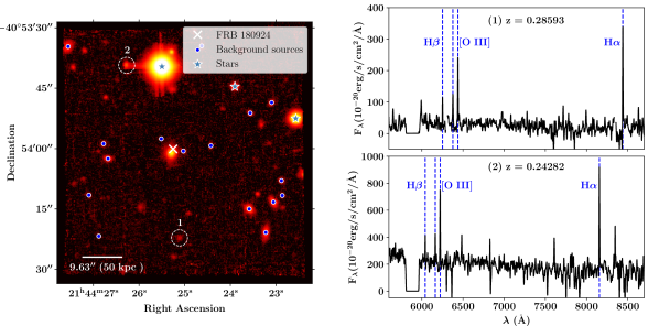
Figure 1: Left: MUSE white light image of the $1\arcmin\times 1\arcmin$ field around the host galaxy of FRB 180924. The circled objects are the two foreground galaxies and the blue dots are background sources identified using MARZ. The blue stars mark the stars in the field. The redshifts of the unmarked sources in the image could not be identified due to their spectra either being noisy or not having a clear correlation with any of the default MARZ template spectra. The white bar at the bottom represents 50 kpc at $z_{\rm host}$. Right: The spectra of sources 1 and 2. Both galaxies show clear H$\alpha$, H$\beta$ and [O III] doublet emission lines which help pinning their redshifts to the values noted above the spectra.

For the galaxies at $0.001<z<0.05$ along the sightline, we turned to the 2MASS survey database (Huchra et al., 2012) for spectroscopic data. This catalog contains galaxy spectra of 83% of the southern sky and is complete to $J<13.75$ with median redshift $z=0.053$. We determined that the galaxy in this catalog with the smallest perpendicular distance to the FRB sightline was 1.04 Mpc (15.2$\arcmin$ angular distance) away, which is far beyond the typical virial radii of galaxy halos. We also found no galaxy within 500 kpc in NearGalCat, the updated nearby galaxy catalog of 869 galaxies within 11 Mpc of the Milky Way which is estimated to be $\sim 40\%$ complete (Karachentsev et al., 2013). Thus, we conclude the $z<0.03$ intervening galaxy halo contribution to ${\rm DM}_{\rm FRB}$ is negligible if not null.

To survey galaxies close to the FRB sightline we used the MUSE integral field unit (Bacon et al., 2010) on the Very Large Telescope (VLT). A set of $4\times 628$ s exposures were obtained on UT 2018 November 5 from program 2102.A-5005 (PI Macquart); another set of $4\times 600$ s exposures were obtained on UT 2019 December 6 from program 0104.A-0411 (PI Tejos). These observations were carried out in the Wide-Field Adaptive Optics (WFM-AO) mode, corresponding to a effective FoV of $1\arcmin\times 1\arcmin$ with a pixelscale of $0.2\arcsec$, and covering a wavelength range of $R\approx 4800-9300$ Å at a resolving power of $\sim 2000-4000$, respectively. After preliminary reduction using the EsoReflex pipeline (Freudling et al., 2013), the frames were flat-field corrected, sky-subtracted and co-added using the CubExtractor package (see Cantalupo et al., 2019, for a description). Sources in the datacube were identified from the white light image, i.e., the cube collapsed along the spectral dimension (see Figure 1), using the Source Extractor of Python (SEP) package (Bertin & Arnouts, 1996; Barbary, 2016). We set minimum threshold of 3 standard deviations above the sky background level and with a minimum area of 10 pixels. Their spectra were extracted from the spaxels within the elliptical apertures whose linear dimensions were twice as large as those returned by SEP. The extraction weighted the flux from the spaxels encircled by the aperture equally. Where the aperture intersected a spatial pixel, the flux from that pixel was scaled down by the fraction of the pixel area within the aperture. Redshifts were identified for each spectrum from the emission features using the Manual and Automatic Redshifting software (MARZ; Hinton et al., 2016). Out of the 72 non-stellar sources identified from the white light image, 19 had their redshifts confidently assigned. These objects are listed in Table 2. The remaining spectra did not have identifiable spectral features (e.g. emission lines). Further relaxing the source detection criteria for SEP increased the number of “sources” but did not increase the number of identified redshifts. From the secure redshifts, we identify two foreground sources from the datacube ($z=0.24282$ and $0.28593$; see Figure 1). Only the closer galaxy is detected in the DES $grizY$ imaging catalog.

Table 2: MUSE and LRIS sources with unambiguous redshifts.

RA	Dec	Redshift	DES ID	r	Separation	Transverse distance
$\deg$	$\deg$			mag	arcmin	kpc
326.10947	-40.89425	0.24282	209914195	22.71	0.40	94
326.10465	-40.90616	0.28593	$\cdots$	$\cdots$	0.37	98
326.10538	-40.90030	0.32157	209914488	20.54	0.01	3
326.10430	-40.90017	0.38406	$\cdots$	$\cdots$	0.04	13
326.11117	-40.90069	0.38407	209914588	22.63	0.26	85
326.09677	-40.90579	0.46956	209914896	22.09	0.52	189
326.10631	-40.89932	0.50086	$\cdots$	$\cdots$	0.06	24
326.09828	-40.90417	0.53556	209914807	21.87	0.40	158
326.09607	-40.90369	0.54431	209914777	22.41	0.47	186
326.09527	-40.90323	0.54464	$\cdots$	$\cdots$	0.49	193
326.11480	-40.89296	0.61709	209914131	22.10	0.60	252
326.10178	-40.89980	0.75084	209914542	24.54	0.16	74
326.09534	-40.90221	0.75097	209914676	23.54	0.47	213
326.10262	-40.89292	0.86432	$\cdots$	$\cdots$	0.44	210
326.09819	-40.89755	0.87372	209914406	23.86	0.36	171
326.11157	-40.89967	1.03010	209914529	24.29	0.28	138
326.09623	-40.89683	1.03477	209914359	24.06	0.46	228
326.11291	-40.90321	1.43899	$\cdots$	$\cdots$	0.40	206
326.11201	-40.90604	2.95747	$\cdots$	$\cdots$	0.47	225
326.09791	-40.93261	0.07221	1.98	209916475	18.69	169

We also obtained spectra of 5 galaxies using the Low Resolution Imaging Spectrograph (LRIS) installed on the Keck telescope on November 8 2020 in the longslit spectroscopy mode. These galaxies were targeted as our analysis indicated they could contribute to ${\rm DM}_{\rm FRB}$(see Section 3.2). We used the “d560” dichroic, 600/4000 grism on the blue side and 600/7500 grating for the red side with $2\times 2$ binning on both detectors. Three of these spectra were exposed for $\sim 700$ s while the other two were exposed for $\sim 300$ s. We could not expose longer on account of bad weather. Of the 5 galaxies, one was confidently assigned a redshift using MARZ and it was determined to be a foreground source ($z=0.07221$; 169 kpc away). We did not detect identifiable emission lines in the remaining 4 low S/N spectra.

3 Methods

3.1 Photometric analysis

We aim at estimating the DM contribution of galaxies that only have photometric redshifts, for which we require several intermediate derived quantities to then compute $\rm DM_{phot,halos}$, the DM contribution of galaxies without spectroscopic redshifts in our sample. Namely, we require photometric redshifts, $z_{\rm phot}$, and halo mass estimates, $M_{\rm halo}$, for every galaxy.

We first estimated the posterior distribution of $z_{\rm phot}$ for each DES galaxy using the EAZY software package (Brammer et al., 2008). Redshifts were only computed for those galaxies which were detected in at least four of the nine filters considered (five from DES and four from WISE) and were estimated in a Bayesian framework using template spectral energy distribution (SED) fitting. We used linear combinations of the templates available in the eazy_v1.3 set and applied magnitude priors on the $r$-band photometry when available (see details in Brammer et al., 2008). When fitting, the redshift was allowed to freely vary between 0.01 and 7 but the priors heavily penalized redshifts higher than 2.

The estimation of halo masses is less direct. Briefly, starting with an estimate for the galaxy’s redshift based on the photometry, we fitted the available fluxes with an SED using the CIGALE software package (Noll et al., 2009; Boquien et al., 2018). We assumed, for simplicity, a delayed-exponential star-formation history with no burst population, a synthetic stellar population prescribed by Bruzual & Charlot (2003), the Chabrier (2003) initial mass function (IMF), dust attenuation models from Calzetti (2001), and dust emission templates from Dale et al. (2014), where the AGN fraction was capped at 20%. This provided an estimate of the stellar mass, $M_{*}$, of the galaxy at a given $z$. We then translate $M_{*}$ to galactic halo mass, $M_{\rm halo}$, using the mean Stellar to Halo Mass Ratio (SHMR) described by Moster et al. (2013) at that $z$. For sources with spectroscopic redshifts, the galaxy redshift is fixed in the CIGALE input. We elaborate on the use of $z_{\rm phot}$ posteriors for the remaining sources in the next subsection.

The uncertainties in the $M_{*}$ estimation and the SHMR relation propagate into the ${\rm DM}_{\rm halos}$ estimate. For each galaxy, we assumed that the $\log M_{*}$ distribution at a given redshift was Gaussian with the mean and standard deviations obtained from CIGALE. Accounting for the error in the SHMR is more involved as it depended on both $M_{*}$ and galaxy redshift. The SHMR is described in Equation 2 of Moster et al. (2013) with 8 parameters. We took the best fit parameters and uncertainties from their Table 1 as the mean and standard deviations of the independent normal distributions that these parameters were sampled from. For simplicity, we ignored any co-variance in these fit parameters (future work will account for this). We then produced a uniform 2D grid of redshift (between 0.03 and 0.35 spaced by 0.01) and $\log M_{*}/{\rm M}_{\odot}$ (between 6 and 11 spaced by 0.005). At each grid point, we sampled the parameter distributions and produced a lookup table of the mean and standard deviations of halo masses that can be realized. Then, to quicken computation, we constructed interpolation functions that mapped the 2D grid to the mean and standard deviation of $\log M_{\rm halo}/{\rm M}_{\odot}$. Figure 2 shows the mean and standard deviations for some representative redshift and stellar mass values. The halo mass distributions were assumed to be Gaussian with the moments given by these interpolation functions.

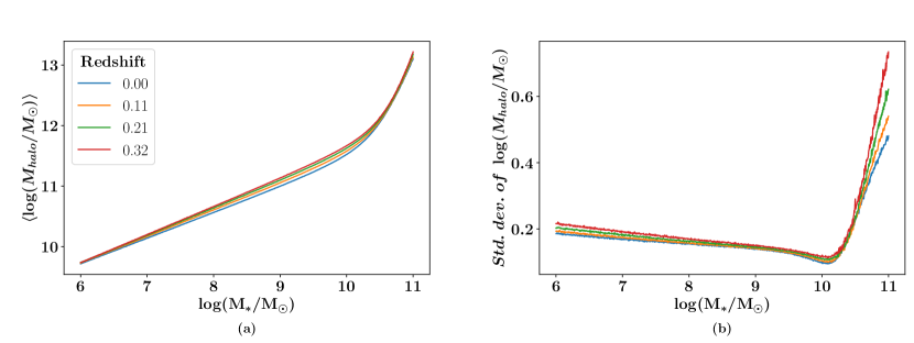
Figure 2: $M_{\rm halo}$ stellar to halo mass ratio (SHMR) mean and standard deviation obtained from sampling the fit parameter space from Moster et al. (2013). The SHMR relation (their eq. 2) contains 8 fit parameters and in this work, we have assumed they are independent and normally distributed. The mean and standard error of these fit parameters were obtained from their Table 1. Using these curves, interpolation functions are constructed to translate ($M_{*}$,z) pairs to $M_{\rm halo}$  distributions.

3.2 Halo contribution to DM

To estimate ${\rm DM}_{\rm halos}$, we performed an analysis similar to the one outlined by Simha et al. (2020) for the FRB 190608 sightline. Briefly, they identified foreground galaxies based on spectroscopic redshifts and estimated halo masses from the available photometry. Then they estimated the line of sight electron number density integral for each intevening halo assuming a model for the baryonic distribution and summed the contributions to yield ${\rm DM}_{\rm halos}$. We emphasize that the redshift serves as a key input to each step of the analysis. In the case of FRB 180924, we modified the procedure to leverage galaxies with $z_{\rm phot}$ as follows (see Figure 3 for a visual flowchart):

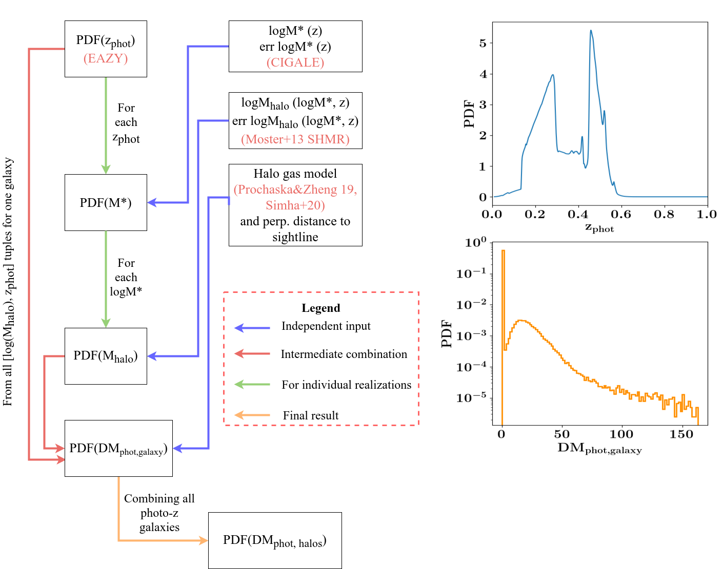
Figure 3: A schematic flowchart of our procedure to estimate $\rm DM_{phot,halos}$. The boxes in the centre with blue arrows emanating from them represent independent inputs into the calculation. These include the stellar mass estimates, the SHMR and the halo gas model. The $z_{\rm phot}$ PDF is also an independent input and an example for one galaxy is shown on the plot on the top right. The sources of these estimates are mentioned in red lettering. The PDF of $\rm DM_{phot,halos}$ is obtained in stages. First, the PDF of stellar masses at each redshift (sampled from the EAZY $z_{\rm phot}$ posterior) is obtained. Then each stellar mass and redshift tuple is translated to halo mass distributions using the Moster et al. (2013) SHMR relation. Compiling all the halo mass and redshift tuples and calculating their DM contribution (using the method outlined in Prochaska & Zheng, 2019; Simha et al., 2020), yields a PDF of DM values for each individual galaxy in our sample. An example of this is shown in the bottom right plot for the same galaxy as the $z_{\rm phot}$ PDF plot. The final PDF of $\rm DM_{phot,halos}$ is estimated by sampling the galaxy DM PDFs and obtaining the distribution of the sum of these samples.

For a given galaxy:

1. We estimated the posterior distributions for $z_{\rm phot}$ and sampled them to produce 1000 realizations.

2. Separately, we allowed the galaxy redshift to vary from 0.03 to 0.35 in a linear grid (spacing 0.01) and estimated the mean and standard deviation of the stellar mass at each grid point using CIGALE.

3. Then, at each redshift realization from step 1, we sampled the $\log M_{*}$ distribution (100 times) obtained using the CIGALE outputs as described in the previous sections.

4. For each stellar mass estimate, we used the 2D interpolation functions to obtain the mean and standard deviation of halo mass. Using these parameters, we produced 10 samples of halo mass values.

5. Combining all the halo mass realizations for all redshift and stellar mass pairs (i.e. $1000\times 100\times 10=10^{6}$ total realizations), we finally produced estimates of DM for each galaxy halo intersecting the sightline (henceforth, $\rm DM_{phot,galaxy}$). $\rm DM_{phot,galaxy}$ values are calculated for each tuple of $M_{\rm halo}$ and $z_{\rm phot}$ realizations as follows:

   1. First the perpendicular distance from the FRB sightline is computed.

   2. Then, assuming the model for electron distribution as described in Simha et al. (2020), $\rm DM_{phot,galaxy}$ is estimated. We assumed that each halo extends to 1 virial radius and the fraction of halo baryons present as hot ($>10^{6}$ K) gas is 0.75. This assumes that 25% of the baryons in the galaxy is in condensed forms (e.g. stars and neutral gas; see Fukugita et al., 1998). While this fraction may vary with halo properties (e.g. Behroozi et al., 2010), we emphasize that this is a relatively conservative maximal model for the CGM of galaxies, i.e. one may consider the estimates as upper limits.

Finally, using the $\rm DM_{phot,galaxy}$ distributions for all galaxies in the sightline, we produced the distribution of their sum, i.e. $\rm DM_{phot,halos}$.

In the fifth step we imposed some bounds on $M_{\rm halo}$ estimates to ensure reasonable values. Namely, the $M_{\rm halo}$ estimated at a particular redshift grid point may not exceed $10^{12.8}~{}{\rm M}_{\odot}$, which is nearing a typical galaxy group halo mass. Exceeding this value is allowed by the uncertainty limits from the SHMR. Therefore, we artificially capped the halo mass estimates to $10^{12.8}~{}{\rm M}_{\odot}$, i.e. any halo mass realization above this limit was set by hand to $10^{12.8}~{}{\rm M}_{\odot}$. Our $\rm DM_{phot,halos}$ distribution was largely unaffected by this choice of the upper limit as an overwhelming majority of galaxies (including the ones within $2\arcmin$ to the sightline) have halo mass estimates much less than this limit. Additionally, it is often the case that the posterior distribution of $z_{\rm phot}$ peaks beyond the FRB host redshift, $z_{\rm host}$= 0.3216. Even in this case there is a non-zero probability of the galactic redshift being below $z_{\rm host}$. For all $z_{\rm phot}$ realizations beyond $z_{\rm host}$, we set $\rm DM_{phot,galaxy}$=$0~{}{\rm pc\,cm^{-3}}$.

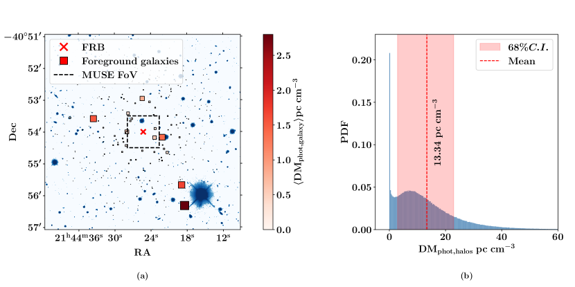
Figure 4: (a) Locations of DES galaxies (excluding those with MUSE and LRIS redshifts) coloured by their average estimates of $\rm DM_{phot,galaxy}$. Both the colors and the sizes of the points are proportional to the mean $\rm DM_{phot,galaxy}$. The background image in blue is the DES $r$-band image of the field. The objects that fall within the MUSE field of view (black, dashed rectangle) do not have spectroscopic redshifts as their spectra did not have identifiable spectral features. (b) A realization of the PDF of $\rm DM_{phot,halos}$ estimated by producing $10^{6}$ realizations of the sum of $\rm DM_{phot,galaxy}$ for all non-spectroscopic galaxies. The histogram counts are normalized to add up to unity. The large spike at 0 ${\rm pc\,cm^{-3}}$ is indicative of the possibility of most of these galaxies being in the background according to their $z_{\rm phot}$ posteriors.

4 Results

Figure 4a shows the average $\rm DM_{phot,galaxy}$ contributed by each of the foreground sources estimated using this method. We excluded all sources for which we have spectroscopic redshifts from MUSE or LRIS. There were $\sim 11000$ DES galaxies in our catalog. We had expected correctly that a large fraction of these sources do not contribute to ${\rm DM}_{\rm halos}$.

Based on these results, we targeted the 5 sources with highest mean $\rm DM_{phot,galaxy}$ using Keck/LRIS ($\S$ 2.2 and we detected line emission from one ($z=0.07221$) of them, thus solidifying its redshift (listed in the last row of Table 2).

Figure 4b shows a realization of the final PDF of $\rm DM_{phot,halos}$ estimated from the 422 galaxies that have a non-zero probability of contributing to the FRB DM. Its mean value is $13$ ${\rm pc\,cm^{-3}}$ and the 68% confidence bounds are $4$ and $23$ ${\rm pc\,cm^{-3}}$. The spike at $0$ ${\rm pc\,cm^{-3}}$ arises from the fact that most galaxies have their redshift posterior distributions peaking beyond the FRB redshift, i.e. the majority of these are likely to have zero contribution to ${\rm DM}_{\rm FRB}$.

Our sample of foreground galaxies with spectroscopic redshifts consists of three galaxies: two from our MUSE datacube and one from our LRIS pointings. One of the MUSE galaxies (z=0.2859) does not have DES/WISE photometry. Therefore, we derived the stellar mass estimate from a pPXF (Cappellari, 2017) fit to its MUSE spectrum and assumed an error of 0.3 dex for $\log M_{*}/{\rm M}_{\odot}$. From these galaxies, we estimated the mean net DM contribution of $7$ ${\rm pc\,cm^{-3}}$with 68% confidence bounds being 3 ${\rm pc\,cm^{-3}}$ and 12 ${\rm pc\,cm^{-3}}$. The bounds were estimated by propagating the uncertainties in the stellar mass and SHMR as described previously but the redshift is fixed.

Thus, the mean ${\rm DM}_{\rm halos}$ estimate, which is the sum of the estimates from the two disjoint samples is 21 ${\rm pc\,cm^{-3}}$ and the 68% confidence limits are 9 ${\rm pc\,cm^{-3}}$ and 32 ${\rm pc\,cm^{-3}}$. The full distribution is shown in Figure 5.

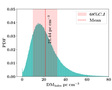
Figure 5: The distribution of ${\rm DM}_{\rm halos}$ estimated using the full sample of foreground galaxies i.e. including galaxies with spectroscopic redshifts from MUSE and LRIS. The galaxies with spectra add 7.1 ${\rm pc\,cm^{-3}}$ to ${\rm DM}_{\rm halos}$ on average, thus shifting the mean value from 13.34 ${\rm pc\,cm^{-3}}$ in Figure 4b to 21.44 ${\rm pc\,cm^{-3}}$.

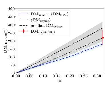
Figure 6: An estimate of ${\rm DM}_{\rm cosmic}$ for the FRB 180924 sightline (blue, solid line) which is a sum of ${\rm DM}_{\rm halos}$ from this analysis and the average diffuse IGM contribution, $\langle{\rm DM}_{\rm IGM}\rangle$. Starting from z = 0, ${\rm DM}_{\rm halos}$ increases as one encounters halos along the sightline and the value at $z_{\rm host}$ is the one estimated in Figure 5. $\langle{\rm DM}_{\rm IGM}\rangle$ increases similarly as more matter is met on average going out towards the FRB. The blue, shaded region corresponds to the 68% confidence interval obtained from the uncertainty in ${\rm DM}_{\rm halos}$. The red point at 220 ${\rm pc\,cm^{-3}}$ is an estimate of $\rm DM_{\rm cosmic,FRB}$  obtained by subtracting the Milky Way and host galaxy contributions from the net DM. The error bar is the net uncertainty in this estimate and corresponds to 50 % uncertainty in each of the subtracted quantities, added in quadrature. The black, solid line is $\langle{\rm DM}_{\rm cosmic}\rangle$ described by the Macquart relation and the gray shaded region represent its scatter ($1\sigma$ limits) due to the filamentary nature of the cosmic web. The black dotted line is the locus of all the median values of ${\rm DM}_{\rm cosmic}$ obtained from the same distribution (Macquart et al., 2020).

5 Discussion and concluding remarks

For FRB 190608, Simha et al. (2020) estimated ${\rm DM}_{\rm halos}$ to be between 7 ${\rm pc\,cm^{-3}}$ and 28 ${\rm pc\,cm^{-3}}$. This corresponded to between 2% and 8% of the net DM and between 5% and 20% of ${\rm DM}_{\rm cosmic}$. In the case of FRB 190608, the theoretical average value, $\langle{\rm DM}_{\rm halos}\rangle$ at $z_{\rm host}$ is 44 ${\rm pc\,cm^{-3}}$, a few times larger than the estimated ${\rm DM}_{\rm halos}$in that sightline. This expectation value is computed assuming $\Lambda$CDM cosmological parameters from Planck Collaboration et al. (2016), a model for the gas density in halos (the same as we have used previously), and the Aemulus halo mass function (HMF; McClintock et al., 2019). The HMF is integrated between $10^{10.3}~{}{\rm M}_{\odot}$ and $10^{16}~{}{\rm M}_{\odot}$.

In the case of FRB 180924, the expected $\langle{\rm DM}_{\rm halos}\rangle$ is 121 ${\rm pc\,cm^{-3}}$ because it is more distant than than FRB 190608. Compared to this, the mean value of ${\rm DM}_{\rm halos}$  estimated in the previous section is just 21 ${\rm pc\,cm^{-3}}$ assuming the same CGM model. Thus, ${\rm DM}_{\rm halos}$ is conclusively lower than average for this sightline, much like FRB 190608.

Figure 6 shows, with a solid blue line, the sum of our ${\rm DM}_{\rm halos}$ estimate and $\langle{\rm DM}_{\rm IGM}\rangle$,the average DM contribution of the diffuse IGM. We define $\langle{\rm DM}_{\rm IGM}\rangle$ as $\langle{\rm DM}_{\rm halos}\rangle$, as computed above, subtracted from $\langle{\rm DM}_{\rm cosmic}\rangle$, i.e. the mean Macquart relation ($\langle{\rm DM}_{\rm IGM}\rangle\equiv\langle{\rm DM}_{\rm cosmic}\rangle-\langle{\rm DM}_{\rm halos}\rangle$). Comparing it to the $\rm DM_{\rm cosmic,FRB}$ estimate (shown as a red point with errors) we see that the two independently computed estimates are indeed consistent. Favored models of the cosmic web indicate that most FRB sightlines in the universe will have few if not zero dark matter halos intersecting them proximally (e.g. Macquart et al., 2020).i.e. if one were to connect the median values of the ${\rm DM}_{\rm cosmic}$ distributions at each redshift, the resulting curve, which can be called the median Macquart relation, lies below the mean curve and is shown as the dotted, black line. Indeed, $\rm DM_{\rm cosmic,FRB}$ is coincident with this median curve. We therefore conclude that FRB 180924 is one such sightline.

We note here that there are indeed other models of gas distribution in the CGM, some of which predict larger dispersion measures, by a factor of a few, from individual halos, (e.g. see Figure 1 of Prochaska & Zheng, 2019). If we were to use any of these models which predict systematically higher DM contributions, both ${\rm DM}_{\rm halos}$ and $\langle{\rm DM}_{\rm halos}\rangle$ would increase by the same factor, and therefore ${\rm DM}_{\rm halos}$ for this sightline would still be lower than average. Simultaneously, our estimate for ${\rm DM}_{\rm cosmic}$ in Figure 6 (the blue line) would decrease when using these models. This is because $\langle{\rm DM}_{\rm IGM}\rangle$ constitutes the majority of the ${\rm DM}_{\rm cosmic}$ estimate and by definition, it decreases with increasing $\langle{\rm DM}_{\rm halos}\rangle$. One must be cautious when performing this exercise however. For instance, with our chosen model of halo gas distribution, we estimate $\langle{\rm DM}_{\rm halos}\rangle$ = 121 ${\rm pc\,cm^{-3}}$. Since $\langle{\rm DM}_{\rm cosmic}\rangle$ = 280 ${\rm pc\,cm^{-3}}$ is independent of this model, doubling $\langle{\rm DM}_{\rm halos}\rangle$ would only leave $\sim 40~{}{\rm pc\,cm^{-3}}$ for $\langle{\rm DM}_{\rm IGM}\rangle$. This is low and likely unrealistic at the host redshift, especially compared to the ${\rm DM}_{\rm IGM}$ estimate using the MCPM method for the FRB 190608 sightline by Simha et al. (2020). Thus, to truly estimate ${\rm DM}_{\rm cosmic}$ one cannot simply use $\langle{\rm DM}_{\rm IGM}\rangle$, and a detailed, semi-empirical model of the cosmic web density is required.

In summary, we have shown that photometric data can be used effectively to constrain ${\rm DM}_{\rm halos}$. While the uncertainty in this endeavor is significant, one can use this as a first step in identifying targets for efficient spectroscopic follow up observations. Having full spectroscopic coverage of the field is undeniably better as the photo-$z$ analysis can misidentify background sources as being in the foreground and vice-versa. In the near future, we intend to obtain spectra of field galaxies within a few degrees of FRB 180924 and perform a full cosmic web analysis, including a direct accounting of the diffuse IGM DM contribution. With upcoming large-scale spectroscopic surveys such as DESI, more FRB fields will have galaxies with precise redshifts and a statistical analysis of multiple FRB fields to constrain cosmic web properties such as the fraction of cosmic baryons will be enabled.

Acknowledgments:

Authors S.S., N.T., J.X.P., and K.G.L. as members of the Fast and Fortunate for FRB Follow-up team, acknowledge support from NSF grants AST-1911140 and AST-1910471. K.G.L. acknowledges support from JSPS KAKENHI Grants JP18H05868 and JP19K14755. K.W.B. acknowledges Australian Research Council (ARC) grant DP180100857. N.T. acknowledges support by FONDECYT grant 11191217. S.C. gratefully acknowledges support from Swiss National Science Foundation grant PP00P2_190092 and from the European Research Council (ERC) under the European Union’s Horizon 2020 research and innovation programme grant agreement No 864361. R.M.S. acknowledges support through Australian Research Council Future Fellowship FT190100155 and Discovery Project DP180100857. The Australian Square Kilometre Array Pathfinder is part of the Australia Telescope National Facility which is managed by CSIRO. Operation of ASKAP is funded by the Australian Government with support from the National Collaborative Research Infrastructure Strategy. ASKAP uses the resources of the Pawsey Supercomputing Centre. Establishment of ASKAP, the Murchison Radio-astronomy Observatory and the Pawsey Supercomputing Centre are initiatives of the Australian Government, with support from the Government of Western Australia and the Science and Industry Endowment Fund. We acknowledge the Wajarri Yamatji as the traditional owners of the Murchison Radio-astronomy Observatory site.

Based on observations collected at the European Southern Observatory under ESO programmes 2102.A-5005 and 0104.A-0411. Spectra were also obtained at the W. M. Keck Observatory, which is operated as a scientific partnership among Caltech, the University of California, and the National Aeronautics and Space Administration (NASA). The Keck Observatory was made possible by the generous financial support of the W. M. Keck Foundation. The authors recognize and acknowledge the very significant cultural role and reverence that the summit of Mauna Kea has always had within the indigenous Hawaiian community. We are most fortunate to have the opportunity to conduct observations from this mountain.

The Python scripts used to perform our analysis are available in our FRB GitHub repository (https://github.com/FRBs/FRB).

References

- Abbott et al. (2018) Abbott, T. M. C., Abdalla, F. B., Allam, S., et al. 2018, ApJS, 239, 18
- Bacon et al. (2010) Bacon, R., Accardo, M., Adjali, L., et al. 2010, in Society of Photo-Optical Instrumentation Engineers (SPIE) Conference Series, Vol. 7735, Ground-based and Airborne Instrumentation for Astronomy III, ed. I. S. McLean, S. K. Ramsay, & H. Takami, 773508
- Bahcall & Spitzer (1969) Bahcall, J. N., & Spitzer, Lyman, J. 1969, ApJ, 156, L63
- Bannister et al. (2019) Bannister, K. W., Deller, A. T., Phillips, C., et al. 2019, Science, 365, 565
- Barbary (2016) Barbary, K. 2016, Journal of Open Source Software, 1, 58
- Behroozi et al. (2010) Behroozi, P. S., Conroy, C., & Wechsler, R. H. 2010, ApJ, 717, 379
- Bertin & Arnouts (1996) Bertin, E., & Arnouts, S. 1996, A&AS, 117, 393
- Boquien et al. (2018) Boquien, M., Burgarella, D., Roehlly, Y., et al. 2018, VizieR Online Data Catalog, J/A+A/622/A103
- Brammer et al. (2008) Brammer, G. B., van Dokkum, P. G., & Coppi, P. 2008, ApJ, 686, 1503
- Bruzual & Charlot (2003) Bruzual, G., & Charlot, S. 2003, MNRAS, 344, 1000
- Calzetti (2001) Calzetti, D. 2001, PASP, 113, 1449
- Cantalupo et al. (2019) Cantalupo, S., Pezzulli, G., Lilly, S. J., et al. 2019, MNRAS, 483, 5188
- Cappellari (2017) Cappellari, M. 2017, MNRAS, 466, 798
- Chabrier (2003) Chabrier, G. 2003, PASP, 115, 763
- Chen & Tinker (2008) Chen, H.-W., & Tinker, J. L. 2008, ApJ, 687, 745
- Chittidi et al. (2020) Chittidi, J. S., Simha, S., Mannings, A., et al. 2020, arXiv e-prints, arXiv:2005.13158
- Cordes & Lazio (2003) Cordes, J. M., & Lazio, T. J. W. 2003, ArXiv Astrophysics e-prints, astro-ph/0301598
- Dale et al. (2014) Dale, D. A., Helou, G., Magdis, G. E., et al. 2014, ApJ, 784, 83
- Freudling et al. (2013) Freudling, W., Romaniello, M., Bramich, D. M., et al. 2013, A&A, 559, A96
- Fukugita (2004) Fukugita, M. 2004, Symposium - International Astronomical Union, 220, 227–232
- Fukugita et al. (1998) Fukugita, M., Hogan, C. J., & Peebles, P. J. E. 1998, ApJ, 503, 518
- Gaia Collaboration et al. (2020) Gaia Collaboration, Brown, A. G. A., Vallenari, A., et al. 2020, arXiv e-prints, arXiv:2012.01533
- Gaia Collaboration et al. (2016) Gaia Collaboration, Prusti, T., de Bruijne, J. H. J., et al. 2016, A&A, 595, A1
- Hinton et al. (2016) Hinton, S. R., Davis, T. M., Lidman, C., Glazebrook, K., & Lewis, G. F. 2016, Astronomy and Computing, 15, 61
- Huchra et al. (2012) Huchra, J. P., Macri, L. M., Masters, K. L., et al. 2012, ApJS, 199, 26
- Hunter (2007) Hunter, J. D. 2007, Computing in Science & Engineering, 9, 90
- Karachentsev et al. (2013) Karachentsev, I. D., Makarov, D. I., & Kaisina, E. I. 2013, AJ, 145, 101
- Law et al. (2020) Law, C. J., Butler, B. J., Prochaska, J. X., et al. 2020, ApJ, 899, 161
- Lorimer et al. (2007) Lorimer, D. R., Bailes, M., McLaughlin, M. A., Narkevic, D. J., & Crawford, F. 2007, Science, 318, 777
- Macquart et al. (2020) Macquart, J. P., Prochaska, J. X., McQuinn, M., et al. 2020, Nature, 581, 391
- Madau & Dickinson (2014) Madau, P., & Dickinson, M. 2014, ARA&A, 52, 415
- McClintock et al. (2019) McClintock, T., Rozo, E., Becker, M. R., et al. 2019, ApJ, 872, 53
- Moster et al. (2013) Moster, B. P., Naab, T., & White, S. D. M. 2013, MNRAS, 428, 3121
- Noll et al. (2009) Noll, S., Burgarella, D., Giovannoli, E., et al. 2009, A&A, 507, 1793
- Oliphant (2006) Oliphant, T. E. 2006, A guide to NumPy, Vol. 1 (Trelgol Publishing USA)
- Planck Collaboration et al. (2016) Planck Collaboration, Ade, P. A. R., Aghanim, N., et al. 2016, A&A, 594, A13
- Price-Whelan et al. (2018) Price-Whelan, A. M., Sipőcz, B. M., Günther, H. M., et al. 2018, AJ, 156, 123
- Prochaska et al. (2011) Prochaska, J. X., Weiner, B., Chen, H. W., Mulchaey, J., & Cooksey, K. 2011, ApJ, 740, 91
- Prochaska & Zheng (2019) Prochaska, J. X., & Zheng, Y. 2019, MNRAS, 485, 648
- Simha et al. (2020) Simha, S., Burchett, J. N., Prochaska, J. X., et al. 2020, ApJ, 901, 134
- Tendulkar et al. (2017) Tendulkar, S. P., Bassa, C. G., Cordes, J. M., et al. 2017, ApJ, 834, L7
- Tumlinson et al. (2013) Tumlinson, J., Thom, C., Werk, J. K., et al. 2013, ApJ, 777, 59
- Virtanen et al. (2020) Virtanen, P., Gommers, R., Oliphant, T. E., et al. 2020, Nature Methods, 17, 261
- Werk et al. (2014) Werk, J. K., Prochaska, J. X., Tumlinson, J., et al. 2014, ApJ, 792, 8
- Wilde et al. (2021) Wilde, M. C., Werk, J. K., Burchett, J. N., et al. 2021, ApJ, 912, 9
- Wright et al. (2010) Wright, E. L., Eisenhardt, P. R. M., Mainzer, A. K., et al. 2010, AJ, 140, 1868