Pion photoproduction in chiral perturbation theory with explicit treatment of the $\boldmath{\Delta(1232)}$ resonance

Abstract

We study the reaction of pion photoproduction on the nucleon in the framework of chiral perturbation theory with explicit $\Delta(1232)$ degrees of freedom. In the covariant approach, we give results up to order $\epsilon^{3}$ in the small scale expansion scheme. Furthermore, we provide $\Delta$-less and $\Delta$-full results obtained in the heavy-baryon scheme to analyze the differences to the covariant approach. Low energy constants are fitted to multipole amplitudes using theoretical truncation errors estimated by a Bayesian approach. We also compare our findings to data of neutral pion production cross sections and polarization asymmetries. The description of the reaction is clearly improved by the explicit treatment of the $\Delta(1232)$ resonance.

I Introduction

In this work, we study the process of pion photoproduction on the nucleon, i.e. $\gamma+N\to\pi+N$, in the framework of chiral perturbation theory ($\chi$PT) with explicit $\Delta$ degrees of freedom. Studying this reaction is motivated by several reasons. First, it is the photoproduction of the lightest hadron. From the theoretical point of view, it is one of the simplest processes involving three different particles, and it thus serves as a test field for more complex reactions. From the experimental point of view, this reaction is quite easily accessible close to threshold and there can be no other hadronic final states due to energy conservation. Therefore, a lot of experimental data on pion photoproduction are available. As an additional motivation, pion photoproduction contributes as a subprocess to more complicated reactions, e.g., in radiative pion photoproduction $\gamma+N\to\gamma+\pi+N$, providing an access to the magnetic moment of the $\Delta$ resonance Rijneveen et al. (2021), or in the interaction of nuclei with electromagnetic probes Pastore et al. (2009); Kölling et al. (2011, 2012); Piarulli et al. (2013); Schiavilla et al. (2019); Krebs et al. (2019).

Pion photoproduction has been a research topic for many years, with the first model-independent approach proposed by Kroll and Ruderman in the 1950s Kroll (1954). Based on general principles, such as Lorentz and gauge invariance, they derived a low-energy theorem for the matrix element of charged pion photoproduction at threshold, which expressed the production amplitudes in terms of a series in the parameter $\mu=M_{\pi}/m_{N}$, where $M_{\pi}$ and $m_{N}$ refer to pion and nucleon masses, respectively. Later on, these predictions were improved De Baenst (1970); Vainshtein and Zakharov (1972) by including the so-called partially conserved axial-vector current hypothesis Nambu (1960); Bernstein et al. (1960); Gell-Mann and Levy (1960) and current algebra Adler and Dashen (1968); Treiman et al. (1972); de Alfaro et al. (1973). Until the 1980s, there was little doubt about the validity of the low-energy predictions. Particularly for the charged production channels, which are dominated by the Kroll-Ruderman term, the results from the theorem matched the available data well. However, new data for the neutral production channel at threshold Mazzucato et al. (1986); Beck et al. (1990) showed a non-negligible disagreement with the theoretical predictions for the $s$-wave electric dipole amplitude $E_{0+}$. A first important success for $\chi$PT was the study of Bernard, Kaiser, Gasser and Meißner Bernard et al. (1991, 1992a) on pion photoproduction, which corrected the low-energy theorems by terms arising from pion loop diagrams. However, these corrections, generated by infrared singularities of the loop integrals, even worsened the agreement with data, which is due to the slow convergence of the chiral expansion in the neutral pion production channel. Therefore, renewed interest in pion photoproduction was awakened in the following years, and multiple experimental groups remeasured pion photo- and electroproduction reactions, see e.g. Welch et al. (1992); van den Brink et al. (1995); Blomqvist et al. (1996); Fuchs et al. (1996); Bergstrom et al. (1996, 1997); Bernstein et al. (1997); Kovash (1997); Distler et al. (1998); Liesenfeld et al. (1999); Korkmaz et al. (1999); Schmidt et al. (2001); Merkel et al. (2002); Baumann (2005); Weis et al. (2008); Merkel (2009); Merkel et al. (2011); Hornidge et al. (2013); Hornidge (2013); Lindgren et al. (2013). In parallel, Bernard et al. worked out all the theoretical details in the different reaction channels within the framework of heavy baryon chiral perturbation theory (HB$\chi$PT) Bernard et al. (1992b, a, c, 1994, 1995, 1996a, 1996b, 1996c, 1996d); Fearing et al. (2000). An improvement of the convergence of the chiral expansion has been achieved by extending the pure $\chi$PT approach by means of dispersion-relation techniques Gasparyan and Lutz (2010).

The new approaches of the so-called infrared renormalization Becher and Leutwyler (1999) and the extended-on-mass-shell scheme (EOMS) Fuchs et al. (2003) enabled the treatment of scattering processes in the pion-nucleon sector in a manifestly covariant framework. Consequently, covariant calculations of $\gamma+N\to\pi+N$ were completed up to the leading loop order $\order{{Q}^{3}}$ in Ref. Bernard et al. (2005) using the infrared renormalization scheme, followed by an analysis of the full one-loop order $\order{{Q}^{4}}$ by Hilt et al. Hilt et al. (2013a, b) in the EOMS scheme.

After it was worked out how to include the $\Delta$ resonance as an explicit degree of freedom into $\chi$PT within the so-called small scale expansion (SSE) scheme Hemmert et al. (1997, 1998), the photoproduction of pions has also been considered in this extended framework. An explicit treatment of the $\Delta$ is of great interest, because the small gap between the pion production threshold and the $\Delta$ mass suggests that effects of the $\Delta$ may become important close above threshold. For example, the $M_{1+}$ multipole receives dominant effects from the $\Delta$ resonance for energies close to the $\Delta$ mass. In SSE, the $\Delta$-nucleon mass split $\Delta\equiv m_{\Delta}-m_{N}$ is considered to be of the same order as the pion mass, i.e. $\Delta\sim M_{\pi}\sim\epsilon$. The first calculation of pion photoproduction with explicit $\Delta$ degrees of freedom was completed in HB$\chi$PT Hemmert et al. (1997), focusing on the neutral production channel close to threshold, which showed only moderate effects of the explicit $\Delta$ treatment. A subsequent HB$\chi$PT study Cawthorne and McGovern (2016) found a more distinct improvement of the description in the HB framework. In the covariant approach, first studies of neutral pion photoproduction were done in Refs. Hiller Blin et al. (2015, 2016); Guerrero Navarro et al. (2019); Guerrero Navarro and Vicente Vacas (2020), finding a substantial improvement in the description of the data compared to the HB approach with explicit $\Delta$s. However, in these works a different power counting Pascalutsa and Phillips (2003) is used, the so-called $\delta$ scheme, in which the $\Delta$-nucleon mass split $\Delta$ is considered to be of one order lower than the pion mass $\Delta\sim\delta,M_{\pi}\sim\delta^{2}$. The motivation for such a counting is given by numerical arguments. Since there is no clear evidence for a faster convergence or better efficiency of one of the two schemes, it is desirable to consider pion photoproduction in the SSE for comparison purposes. Note, however, that the low energy constants (LECs) of the two approaches cannot be compared directly, because their numerical values are scheme-dependent. Comparing the results in two counting schemes can be done only in terms of quality of the data description.

We study pion photoproduction in both heavy baryon and covariant formalisms of chiral effective field theory. We also analyze the effects of explicit $\Delta$ degrees of freedom by taking into account their leading-order and next-to-leading order contributions in the covariant formalism of $\chi$PT within the EOMS scheme. To estimate theoretical uncertainties of observables and LECs, we use a Bayesian model Furnstahl et al. (2015); Melendez et al. (2017); Epelbaum et al. (2020).

First, we study the $\Delta$-less case up to order ${Q}^{3}$, which has been considered before Bernard et al. (2005); Hilt et al. (2013a, b). Recent studies were mainly focused on the covariant approach, so we provide a detailed comparison of the two formalisms in order to analyze the difference in convergence and data description. In particular, we compare the obtained LECs in terms of the effects generated by the infrared regular (IR) parts of the integrals. The extraction of the heavy baryon LECs is very important for the use in the few-body applications such as calculation of the nuclear electroweak currents.

Next, we upgrade the covariant calculation to leading-order $\Delta$ tree contributions employing the SSE, which has been used for studies of other reactions such as pion-nucleon scattering and Compton scattering, see e.g. Refs. Siemens et al. (2016, 2017); Thürmann et al. (2021). We also discuss the differences to the $\Delta$-less case in terms of resonance saturation. Moreover, we provide results for the reaction $\gamma+N\to\pi+N$ up to leading $\Delta$-full loop order for the first time. In comparison to the study of Ref. Hiller Blin et al. (2016), we take into account loop diagrams including up to three $\Delta$ propagators, which give rise to significant contributions to the amplitude while maintaining gauge invariance. Furthermore, we give an estimate for the subleading $\gamma N\Delta$ coupling constant $h_{1}$. A qualitative comparison to the aforementioned studies in the $\delta$-scheme is given. Furthermore, we compare some of our results to recent high-precision data in the neutral pion production channel Hornidge et al. (2013); Hornidge (2013, ).

Our paper is structured as follows. In section II, we introduce the basic formalism, such as kinematics, isospin/spin decomposition of the matrix elements and calculation of multipole amplitudes and observables. In section III, we list all terms of the effective Lagrangian relevant for our calculation and discuss the employed power counting scheme. Subsequently, we discuss renormalization in section IV. We present our results in section V and conclude with a short summary in section VI.

II Formalism

In this section, we briefly introduce our notation for kinematics, isospin and spin decomposition as well as the calculation of multipole amplitudes and observables. Pion photoproduction

$$\gamma(\lambda,k)+N_{i}(s,p)\to\pi_{c}(q)+N_{j}(s^{\prime},p^{\prime})$$ (1)

is a reaction where a pion is produced by absorption of a photon from a nucleon. Here, $p(p^{\prime})$, $s(s^{\prime})$ and $i(j)$ are momentum, helicity and isospin index of the incoming (outgoing) nucleon, $k$ and $\lambda$ are momentum and helicity of the photon, and $q$ and $c$ are momentum and isospin index of the pion, respectively. The kinematics of the reaction is uniquely defined by two Lorentz-invariant Mandelstam variables

$$s=(p+k)^{2}=(p^{\prime}+q)^{2},\quad t=(p-p^{\prime})^{2}=(k-q)^{2}\,.$$ (2)

The energies of the photon $\omega$ and the pion $E_{\pi}$ in the center-of-mass (CM) frame expressed in terms of the Mandelstam variables read

$$\omega=\frac{s-m_{N}^{2}}{2\sqrt{s}},\quad E_{\pi}=\frac{s+M_{\pi}^{2}-m_{N}^{2}}{2\sqrt{s}}.$$ (3)

In the laboratory frame, the photon energy can be calculated from the total CM energy using

$$\omega_{\text{lab}}=\frac{s-m_{N}^{2}}{2m_{N}}.$$ (4)

Furthermore, we define the scattering angle $\theta$ via $\lvert\boldsymbol{k}\rvert\,\lvert\boldsymbol{q}\rvert\cos(\theta)=\boldsymbol{k}\cdot\boldsymbol{q}$, such that

$$t=M_{\pi}^{2}-2(\omega E_{\pi}-\lvert\boldsymbol{k}\rvert\,\lvert\boldsymbol{q}\rvert\cos(\theta)).$$ (5)

The pion production threshold lies at the CM energy of $\sqrt{s}=m_{N}+M_{\pi}$. In the HB formalism, an explicit $1/m_{N}$ expansion of the amplitude is performed. Expanding Eq. (3) in terms of $1/m_{N}$, we can derive an approximate relation between photon and pion CM energy

$$\omega=E_{\pi}-\frac{M_{\pi}^{2}}{2m_{N}}+\order{\frac{1}{m_{N}^{2}}}.$$ (6)

Thus, in the HB formalism, we express all kinematic quantities in terms of the pion energy $E_{\pi}$.

In the isospin space, the matrix elements of pion photoproduction can be parameterized in terms of three independent structures

$$T_{\gamma N\to\pi N}^{c}=\delta_{c3}\,T^{(+)}_{\gamma N}+\tau_{c}\,T^{(0)}_{\gamma N}+\textup{i}\varepsilon_{c3a}\,\tau_{a}\,T^{(-)}_{\gamma N},$$ (7)

where $\tau^{i}$ are the Pauli matrices in the isospin space. In Eq. (7), $T$ can refer to the pion photoproduction amplitude in any representation including the photoproduction multipoles.

The matrix elements for the four physical pion photoproduction reaction channels

$$\gamma p\to\pi^{0}p,\quad\gamma p\to\pi^{+}n,\quad\gamma n\to\pi^{0}n,\quad\gamma n\to\pi^{-}p$$ (8)

can be obtained from the three isospin structures by using the following relations

$$T_{\gamma p\to\pi^{0}p} =T^{(+)}_{\gamma N}+T^{(0)}_{\gamma N}, \quad T_{\gamma p\to\pi^{+}n} =\sqrt{2}(T^{(0)}_{\gamma N}+T^{(-)}_{\gamma N}),$$

$$T_{\gamma n\to\pi^{0}n} =T^{(+)}_{\gamma N}-T^{(0)}_{\gamma N}, \quad T_{\gamma n\to\pi^{-}p} =\sqrt{2}(T^{(0)}_{\gamma N}-T^{(-)}_{\gamma N}).$$ (9)

Another commonly used decomposition of the pion photoproduction amplitude is the so-called isospin parametrization in terms of the three amplitudes $T_{\gamma N}^{(\frac{3}{2})},T_{\gamma p}^{(\frac{1}{2})},T_{\gamma n}^{(\frac{1}{2})}$ where the production amplitudes $T_{\gamma N}^{(I)}$ are related to the $T_{\gamma N}^{(0,\pm)}$ via

$$T_{\gamma N}^{(\frac{3}{2})} =T_{\gamma p}^{(\frac{3}{2})}=T_{\gamma n}^{(\frac{3}{2})}=T_{\gamma N}^{(+)}-T_{\gamma N}^{(-)},$$

$$T_{\gamma p}^{(\frac{1}{2})} =T_{\gamma N}^{(0)}+\frac{1}{3}T_{\gamma N}^{(+)}+\frac{2}{3}T_{\gamma N}^{(-)},\quad T_{\gamma n}^{(\frac{1}{2})}=T_{\gamma N}^{(0)}-\frac{1}{3}T_{\gamma N}^{(+)}-\frac{2}{3}T_{\gamma N}^{(-)}.$$ (10)

The isospin parametrization is a natural choice when working in the isospin symmetric case of $\chi$PT, thus we perform the fits in this work using this basis. For comparison with experimental results, the decomposition (9) in terms of the physical reaction channels is required.

The pion photoproduction amplitude $\mathcal{M}=\epsilon^{\mu}\mathcal{M}_{\mu}$, where $\epsilon^{\mu}$ is the polarization vector of the photon, can be parameterized in terms of the so-called Ball amplitudes Ball (1961)

$$\mathcal{M}^{\mu}=\sum\limits_{i=1}^{8}\bar{u}(p^{\prime})B_{i}V_{i}^{\mu}u(p).$$ (11)

Here the coefficients $B_{i}$ are scalar functions of the Mandelstam variables, and the basis structures $V_{i}^{\mu}$ comprise all independent matrices that can be formed using gamma matrices and the polarization vector, they read

$$V_{1}^{\mu} =\gamma^{\mu}\gamma_{5}, V_{2}^{\mu} =\gamma_{5}P^{\mu}, V_{3}^{\mu} =\gamma_{5}q^{\mu}, V_{4}^{\mu} =\gamma_{5}k^{\mu},$$

$$V_{5}^{\mu} =\gamma^{\mu}\not{k}\gamma_{5}, V_{6}^{\mu} =\not{k}\gamma_{5}P^{\mu}, V_{7}^{\mu} =\not{k}\gamma_{5}q^{\mu}, V_{8}^{\mu} =\not{k}\gamma_{5}k^{\mu},$$ (12)

where $P=1/2\,(p+p^{\prime})$. Note that the set of amplitudes (11)-(12) is not minimal. Imposing transversality $k_{\mu}\mathcal{M}^{\mu}=0$ leads to the following conditions

$$B_{1}+B_{6}\,k\cdot P+B_{7}\,k\cdot q+B_{8}\,k^{2}=0,\quad B_{2}\,k\cdot P+B_{3}\,k\cdot q+B_{4}\,k^{2}+B_{5}\,k^{2}=0.$$ (13)

Thus, current conservation reduces the number of basis structures to six. Only four structures remain for real pion photoproduction due to the additional constraints $\epsilon\cdot k=0$ and $k^{2}=0$, which can be chosen in the form of CGLN amplitudes Chew et al. (1957):

$$\mathcal{M}^{\mu} =\sum\limits_{i=1}^{4}\bar{u}(p^{\prime})A_{i}M_{i}^{\mu}u(p),$$

$$M_{1}^{\mu} =-\tfrac{\textup{i}}{2}\gamma_{5}(\gamma^{\mu}\not{k}-\not{k}\gamma^{\mu}),$$

$$M_{2}^{\mu} =2\textup{i}\gamma_{5}\left(P^{\mu}k\cdot(q-\tfrac{1}{2}k)-(q^{\mu}-\tfrac{1}{2}k^{\mu})k\cdot P\right),$$

$$M_{3}^{\mu} =-\textup{i}\gamma_{5}(\gamma^{\mu}k\cdot q-\not{k}q^{\mu}),$$

$$M_{4}^{\mu} =-2\textup{i}\gamma_{5}(\gamma^{\mu}k\cdot P-\not{k}P^{\mu})-2m_{N}M_{1}^{\mu}.$$ (14)

In the CM frame, one can conveniently introduce another set of amplitudes in the gauge $\epsilon^{0}=0$ Chew et al. (1957):

$$\epsilon_{\mu}\bar{u}(p^{\prime})\left(\sum_{i=1}^{4}A_{i}M_{i}^{\mu}\right)u(p)=\frac{4\uppi\sqrt{s}}{m_{N}}\chi^{\dagger}_{f}\,\mathcal{F}\,\chi_{i}\,,$$ (15)

with

$$\mathcal{F}=\textup{i}\,\boldsymbol{\sigma}\,\cdot\boldsymbol{\epsilon}\,\mathcal{F}_{1}+\frac{\boldsymbol{\sigma}\cdot\boldsymbol{q}\,\boldsymbol{\sigma}\cdot(\boldsymbol{k}\crossproduct\boldsymbol{\epsilon})}{\absolutevalue{\boldsymbol{q}}\,\absolutevalue{\boldsymbol{k}}}\,\mathcal{F}_{2}+\textup{i}\frac{\boldsymbol{\sigma}\cdot\boldsymbol{k}\,\boldsymbol{q}\cdot\boldsymbol{\epsilon}}{\absolutevalue{\boldsymbol{q}}\,\absolutevalue{\boldsymbol{k}}}\,\mathcal{F}_{3}+\textup{i}\frac{\boldsymbol{\sigma}\cdot\boldsymbol{q}\,\boldsymbol{q}\cdot\boldsymbol{\epsilon}}{\absolutevalue{\boldsymbol{q}}^{2}}\,\mathcal{F}_{4},$$ (16)

where $\boldsymbol{\sigma}$ are the Pauli matrices in spin space and $\chi_{i}$ ($\chi^{\dagger}_{f}$) is the Pauli spinor of the initial (final) nucleon.

The $\mathcal{F}_{i}$’s can be expanded in a multipole series Chew et al. (1957); Ball (1961):

$$\mathcal{F}_{1} =\sum_{l=0}^{\infty}\left\{[l\,M_{l+}+E_{l+}]P^{\prime}_{l+1}(x)+[(l+1)M_{l-}+E_{l-}]P^{\prime}_{l-1}(x)\right\},$$

$$\mathcal{F}_{2} =\sum_{l=1}^{\infty}[(l+1)M_{l+}+lM_{l-}]P^{\prime}_{l}(x),$$

$$\mathcal{F}_{3} =\sum_{l=1}^{\infty}\left\{[E_{l+}-M_{l+}]P^{\prime\prime}_{l+1}(x)+[E_{l-}+M_{l-}]P^{\prime\prime}_{l-1}(x)\right\},$$

$$\mathcal{F}_{4} =\sum_{l=2}^{\infty}[M_{l+}-E_{l+}-M_{l-}-E_{l-}]P^{\prime\prime}_{l}(x),$$ (17)

where $x=\cos(\theta)$, $P_{l}(x)$ is a Legendre polynomial of degree $l$, $P^{\prime}_{l}(x)=\derivative{P_{l}}{x}(x)$ is its first derivative, $P^{\prime\prime}_{l}(x)$ is the second derivative with respect to $x$ and $l$ is the orbital angular momentum of the outgoing pion-nucleon system. The subscript $\pm$ denotes the total angular momentum $j=l\pm 1/2$. Equation (17) can be inverted:

$$E_{l+} =\int\limits_{-1}^{1}\frac{\differential x}{2(l+1)}\left[P_{l}\mathcal{F}_{1}-P_{l+1}\mathcal{F}_{2}+\frac{l}{2l+1}(P_{l-1}-P_{l+1})\mathcal{F}_{3}+\frac{l+1}{2l+3}(P_{l}-P_{l+2})\mathcal{F}_{4}\right],$$

$$E_{l-} =\int\limits_{-1}^{1}\frac{\differential x}{2l}\left[P_{l}\mathcal{F}_{1}-P_{l-1}\mathcal{F}_{2}-\frac{l+1}{2l+1}(P_{l-1}-P_{l+1})\mathcal{F}_{3}+\frac{l}{2l-1}(P_{l}-P_{l-2})\mathcal{F}_{4}\right],$$

$$M_{l+} =\int\limits_{-1}^{1}\frac{\differential x}{2(l+1)}\left[P_{l}\mathcal{F}_{1}-P_{l+1}\mathcal{F}_{2}-\frac{1}{2l+1}(P_{l-1}-P_{l+1})\mathcal{F}_{3}\right],$$

$$M_{l-} =\int\limits_{-1}^{1}\frac{\differential x}{2l}\left[-P_{l}\mathcal{F}_{1}+P_{l-1}\mathcal{F}_{2}+\frac{1}{2l+1}(P_{l-1}-P_{l+1})\mathcal{F}_{3}\right]\,.$$ (18)

Here, we suppress the $x$-dependence of the Legendre polynomials $P_{l}$ for the sake of brevity.

To calculate multipole amplitudes, we proceed as follows: first, we express the pion photoproduction amplitude in terms of the Ball amplitudes (Eq. (11)). Then, we rewrite the $B_{i}$’s in terms of $A_{i}$’s to obtain the representation of the amplitude in the minimal basis (Eq. (14)). Finally, we use the coefficients $A_{i}$ to calculate $\mathcal{F}_{1}-\mathcal{F}_{4}$. The relations between these representations are given in Appendix A.

Next, we provide the expressions for the unpolarized differential cross section and linear polarization asymmetry. The differential cross section for pion photoproduction is given by

$$\derivative{\sigma}{\Omega}=\frac{1}{64\uppi^{2}s}\frac{\absolutevalue{\boldsymbol{q}}}{\absolutevalue{\boldsymbol{k}}}\absolutevalue{\overline{\mathcal{M}}}^{2},$$ (19)

with the unpolarized squared matrix element $\absolutevalue{\overline{\mathcal{M}}}^{2}$

$$\absolutevalue{\overline{\mathcal{M}}}^{2}=\frac{1}{4}\sum\limits_{\lambda=-1}^{1}\sum\limits_{s,s^{\prime}=-1}^{1}\absolutevalue{\epsilon_{\mu}(k,\lambda)\mathcal{M}^{\mu}(k,p,s,p^{\prime},s^{\prime},q)}^{2},$$ (20)

where again $\lambda$ is the helicity of the photon, $s$ ($s^{\prime}$) is the spin of the incoming (outgoing) nucleon and the factor of 1/4 arises from averaging over helicity and spin of the incoming particles. The linearly polarized photon asymmetry $\Sigma$ is given by

$$\Sigma=\frac{\differential\sigma_{\perp}-\differential\sigma_{\parallel}}{\differential\sigma_{\perp}+\differential\sigma_{\parallel}}\,,$$ (21)

where $\differential\sigma_{\perp}$ and $\differential\sigma_{\parallel}$ refer to the differential cross section for photon polarizations perpendicular and parallel to the reaction plane, respectively.

III Effective Lagrangian and Power Counting

The calculation of observables in chiral perturbation theory is based on Feynman rules derived from the effective Lagrangian. In general, it contains an infinite number of terms with a rising number of derivatives and/or pion masses. At the maximal order we are working, the terms of the effective Lagrangian relevant for the calculation of pion photoproduction read

$$\mathcal{L}_{\text{eff}}=\mathcal{L}_{\pi\pi}^{(2)}+\mathcal{L}_{\pi\pi}^{(4)}+\mathcal{L}_{\pi N}^{(1)}+\mathcal{L}_{\pi N}^{(2)}+\mathcal{L}_{\pi N}^{(3)}+\mathcal{L}_{\pi N\Delta}^{(1)}+\mathcal{L}_{\pi N\Delta}^{(2)}+\mathcal{L}_{\pi N\Delta}^{(3)}+\mathcal{L}_{\pi\Delta}^{(1)}+\mathcal{L}_{\pi\Delta}^{(2)},$$ (22)

where we do not distinguish between HB and covariant notation at this point.

In the mesonic sector, the building blocks are the pion field $U=u^{2}$ with

$$U(x)=1+\textup{i}\frac{\boldsymbol{\tau}\cdot\boldsymbol{\pi}}{F}-\frac{\pi^{2}}{2F^{2}}-\textup{i}\upalpha\frac{\pi^{2}\,\boldsymbol{\tau}\cdot\boldsymbol{\pi}}{F^{3}}+\left(\upalpha-\tfrac{1}{8}\right)\frac{\pi^{4}}{F^{4}}+\order{\pi^{5}},$$ (23)

where $F$ is the pion decay constant in the chiral limit and $\upalpha$ is an arbitrary unphysical parameter from the parametrization of the pion field. The covariant derivative acting on the pion field $\nabla_{\mu}$ is defined as

$$\nabla_{\mu}U=\partial_{\mu}U-\textup{i}r_{\mu}U+\textup{i}Ul_{\mu},\quad l_{\mu}=v_{\mu}-a_{\mu},\quad r_{\mu}=v_{\mu}+a_{\mu},$$ (24)

where $v_{\mu}=-eQ_{N}A_{\mu}=-e\frac{\mathds{1}+\textsf{\leavevmode{t}}_{3}}{2}A_{\mu}$ is the vector source with the electric charge $e\approx$0.303$$ and the electromagnetic field $A_{\mu}$, and $a_{\mu}$ is the axial source. Furthermore, we introduce $\chi=\operatorname{diag}(M^{2},M^{2})$ and $M$ is the pion mass to leading order in quark masses. We also introduce the field combinations

$$\chi_{\pm}=u^{\dagger}\chi u^{\dagger}\pm u\chi^{\dagger}u,\quad F_{L}^{\mu\nu}=\partial^{\mu}l^{\nu}-\partial^{\nu}l^{\mu}-\textup{i}[l^{\mu},l^{\nu}],\quad F_{R}^{\mu\nu}=\partial^{\mu}r^{\nu}-\partial^{\nu}r^{\mu}-\textup{i}[r^{\mu},r^{\nu}].$$ (25)

The relevant parts of the leading and next-to-leading pionic Lagrangian read Gasser and Leutwyler (1984)

$$\mathcal{L}_{\pi\pi}^{(2)} =\frac{F^{2}}{4}\tr\left(\nabla_{\mu}U\nabla^{\mu}U^{\dagger}\right)+\frac{F^{2}}{4}\tr\left(\chi_{+}\right),$$

$$\mathcal{L}_{\pi\pi}^{(4)} =\frac{l_{3}}{16}\tr(\chi_{+})^{2}+\frac{l_{4}}{16}\left(2\tr(\nabla_{\mu}U(\nabla^{\mu}U)^{\dagger})\tr(\chi_{+})+\tr(2((\chi U^{\dagger})^{2}+(U\chi^{\dagger})^{2})-4\chi^{\dagger}\chi-\chi_{-}^{2})\right)$$

$$+\textup{i}\frac{l_{6}}{2}\tr\left(F_{R,\mu\nu}\nabla^{\mu}U(\nabla^{\nu}U)^{\dagger}+F_{L,\mu\nu}(\nabla^{\mu}U)^{\dagger}\nabla^{\nu}U\right).$$ (26)

Introducing nucleons, we give the definitions of

$$D_{\mu} =\partial_{\mu}-\Gamma_{\mu},\quad\Gamma_{\mu}=\frac{1}{2}\left\{u^{\dagger}(\partial_{\mu}-\textup{i}r_{\mu})u+u(\partial_{\mu}-\textup{i}l_{\mu})u^{\dagger}\right\},\quad u_{\mu}=\textup{i}(u^{\dagger}(\partial_{\mu}-\textup{i}r_{\mu})u-u(\partial_{\mu}-\textup{i}l_{\mu})u^{\dagger}),$$

$$F_{\mu\nu}^{\pm} =u^{\dagger}F_{\mu\nu}^{R}u\pm uF_{\mu\nu}^{L}u^{\dagger},\quad\tilde{F}_{\mu\nu}^{\pm}=F_{\mu\nu}^{\pm}-\frac{1}{2}\operatorname{Tr}(F_{\mu\nu}^{\pm}).$$ (27)

The leading order pion-nucleon Lagrangian in the covariant approach is given by

$$\mathcal{L}_{\pi N}^{(1)}=\bar{\Psi}_{N} \left(\textup{i}\not{D}-m+\frac{g}{2}\not{u}\gamma_{5}\right)\Psi_{N},$$ (28)

where $m$ and $g$ are the bare nucleon mass and axial coupling constant. Other relevant parts of the covariant $\pi N$ Lagrangian read (see, e.g., Ref. Fettes et al. (2000))

$$\mathcal{L}_{\pi N}^{(2)}=\bar{\Psi}_{N} \left\{c_{1}\tr(\chi_{+})+\frac{c_{6}}{8m_{N}}F_{\mu\nu}^{+}\sigma^{\mu\nu}+\frac{c_{7}}{8m_{N}}\tr(F_{\mu\nu}^{+})\sigma^{\mu\nu}\right\}\Psi_{N},$$

$$\mathcal{L}^{(3)}_{\pi N}=\bar{\Psi}_{N} \left\{\frac{d_{6}}{2m_{N}}(\textup{i}\left[D^{\mu},\tilde{F}_{\mu\nu}^{+}\right]D^{\nu}+\text{h.c.})+\frac{d_{7}}{2m_{N}}(\textup{i}\left[D^{\mu},\tr(F_{\mu\nu}^{+})\right]D^{\nu}+\text{h.c.})+\frac{d_{8}}{2m_{N}}(\textup{i}\textsf{\leavevmode{e}}^{\mu\nu\alpha\beta}\tr(\tilde{F}_{\mu\nu}^{+}u_{\alpha})D_{\beta}+\text{h.c.})\right.$$

$$+\frac{d_{9}}{2m_{N}}(\textup{i}\textsf{\leavevmode{e}}^{\mu\nu\alpha\beta}\tr(F_{\mu\nu}^{+})u_{\alpha}D_{\beta}+\text{h.c.})+\frac{d_{16}}{2}\gamma^{\mu}\gamma_{5}\tr(\chi_{+})u_{\mu}+\textup{i}\frac{d_{18}}{2}\gamma^{\mu}\gamma_{5}\left[D_{\mu},\chi_{-}\right]$$

$$\left.-\frac{d_{20}}{8m_{N}^{2}}(\textup{i}\gamma^{\mu}\gamma_{5}\left[\tilde{F}_{\mu\nu}^{+},u_{\alpha}\right]D^{\alpha\nu}+\text{h.c.})+\textup{i}\frac{d_{21}}{2}\gamma^{\mu}\gamma_{5}\left[\tilde{F}_{\mu\nu}^{+},u^{\nu}\right]+\frac{d_{22}}{2}\gamma^{\mu}\gamma_{5}\left[D^{\nu},F_{\mu\nu}^{-}\right]\ \right\}\Psi_{N},$$

with $\sigma^{\mu\nu}=\frac{\textup{i}}{2}[\gamma^{\mu},\gamma^{\nu}]$. We use the convention $\textsf{\leavevmode{e}}^{0123}=-1$.

In the heavy baryon formalism, the nucleon momentum is split according to

$$p_{\mu}=m_{N}v_{\mu}+P_{\mu},$$ (29)

where the first part is a large piece close to the on-shell kinematics and the second part $P_{\mu}$ is a soft residual contribution $v\cdot P\ll m_{N}$. The vector $v_{\mu}$ is the four-velocity of the nucleon with the properties $v^{2}=1,v^{0}\geq 1$ and can be conveniently chosen as $v=(1,0,0,0)$. The nucleon field $\Psi_{N}$ is split into the so-called light and heavy fields

$$N_{v}(x)=\operatorname{e}^{\textup{i}m_{N}v\cdot x}P_{v}^{+}\Psi_{N}(x)\mbox{\quad and\quad}h_{v}(x)=\operatorname{e}^{\textup{i}m_{N}v\cdot x}P_{v}^{-}\Psi_{N}(x),$$ (30)

which are eigenstates of $\not{v}$, with the projectors

$$P_{v}^{\pm}=\frac{1}{2}(1\pm\not{v}).$$ (31)

In the heavy baryon formalism, any bilinear $\bar{\Psi}\Gamma\Psi$ with $\Gamma\in\{1,\gamma_{5},\gamma_{\mu},\gamma_{5}\gamma_{\mu},\sigma_{\mu\nu}\}$ can be expressed in terms of the velocity $v^{\mu}$ and the Pauli-Lubanski spin vector

$$S_{\mu}=\frac{\textup{i}}{2}\gamma_{5}\sigma_{\mu\nu}v^{\nu}\,.$$ (32)

The relevant terms of the Lagrangians up to third order read Fettes et al. (2000)

$$\hat{\mathcal{L}}_{\pi N}^{(1)}= \,\bar{N}\left(\textup{i}v\cdot D+g\,S\cdot u\right)N\,,$$

$$\hat{\mathcal{L}}_{\pi N}^{(2)}= \,\bar{N}\left(c_{1}\tr(\chi_{+})-\frac{\textup{i}}{4m_{N}}\left[\hat{c}_{6}\left[S^{\mu},S^{\nu}\right]F_{\mu\nu}^{+}+\hat{c}_{7}\left[S^{\mu},S^{\nu}\right]\tr(F_{\mu\nu}^{+})\right]\right)N\,,$$

$$\hat{\mathcal{L}}_{\pi N}^{(3)}= \,\bar{N}\left(\hat{d}_{6}\left[D^{\mu},\tilde{F}_{\mu\nu}^{+}\right]v^{\nu}+\hat{d}_{7}\left[D^{\mu},\tr(F_{\mu\nu}^{+})\right]v^{\nu}+\hat{d}_{8}\tr(\tilde{F}_{\mu\nu}^{+}u_{\alpha})\textsf{\leavevmode{e}}^{\mu\nu\alpha\beta}v_{\beta}+\hat{d}_{9}\tr(F_{\mu\nu}^{+})u_{\alpha}\textsf{\leavevmode{e}}^{\mu\nu\alpha\beta}v_{\beta}\right.$$

$$\left.\quad+\hat{d}_{16}\,S\cdot u\tr(\chi_{+})+\textup{i}\hat{d}_{18}\left[S\cdot D,\chi_{-}\right]+\textup{i}\hat{d}_{20}S^{\mu}v^{\nu}\left[\tilde{F}_{\mu\nu}^{+},v\cdot u\right]+\textup{i}\hat{d}_{21}S^{\mu}\left[\tilde{F}_{\mu\nu}^{+},u^{\nu}\right]+\hat{d}_{22}S^{\mu}\left[D^{\nu},F_{\mu\nu}^{-}\right]\right)N$$

$$+\frac{1}{2m_{N}}\bar{N}\left((v\cdot D)^{2}-D^{2}-\textup{i}g\left\{S\cdot D,v\cdot u\right\}\right)N\,.$$ (33)

The prefactor of $1/m_{N}$ in the $c_{i}$ parts in $\hat{\mathcal{L}}_{\pi N}^{(2)}$ should not be interpreted as a $1/m_{N}$ correction; it originates from the definition of the constants $\hat{c}_{6}$ and $\hat{c}_{7}$, which are dimensionless when defined this way. Unlike the usual treatment of the single nucleon sector in the literature, we from now on consider the $1/m_{N}$ corrections as $1/m_{N}\sim 1/\Lambda^{2}$, where $\Lambda$ is the hard scale (see below), so that they start to appear at the third instead of the second order. The $1/m_{N}^{2}$ are, therefore, shifted beyond the order we are working. This is a common practice in studies of the nuclear forces Epelbaum et al. (2009) and is referred to as $NN$ counting in this work. Also, note that the heavy baryon LECs $\hat{c}_{6}$ and $\hat{c}_{7}$ are not the same as the covariant constants, but they absorb $1/m_{N}$-shifts from the leading order Lagrangian via $\hat{c}_{6}=c_{6}+1,\hat{c}_{7}=c_{7}$.

The $\Delta$ resonance is introduced as an explicit degree of freedom by an isospin-$3/2$ Rarita-Schwinger spinor $\bar{\Psi}_{\Delta,i}^{\mu}$, which satisfies $\tau_{i}\Psi_{\Delta,\mu}^{i}=0$ Hemmert et al. (1998). Given the following definitions:

$$D^{ij}_{\mu}=\partial_{\mu}\delta^{ij}+\Gamma^{ij}_{\mu},\quad\Gamma^{ij}_{\mu}=\delta^{ij}\Gamma_{\mu}-\textup{i}\textsf{\leavevmode{e}}^{ijk}\tr(\tau_{k}\Gamma^{\mu}),\quad u^{ij}_{\mu}=\xi^{ik}_{3/2}\,u_{\mu}\,\xi^{kj}_{3/2}$$ (34)

with the isospin projectors

$$\xi_{ij}^{3/2}=\frac{2}{3}\delta_{ij}-\frac{\textup{i}}{3}\textsf{\leavevmode{e}}_{ijk}\tau_{k},\quad\xi_{ij}^{1/2}=\frac{1}{3}\delta_{ij}+\frac{\textup{i}}{3}\textsf{\leavevmode{e}}_{ijk}\tau_{k},$$ (35)

the leading covariant $\pi\Delta$-Lagrangian reads Hemmert et al. (1998); Hemmert (1999)

$$\mathcal{L}^{(1)}_{\pi\Delta}= -\bar{\Psi}_{\Delta,i}^{\mu}\left\{(\textup{i}\not{D}^{ij}-\mathring{m}_{\Delta}\delta^{ij})g_{\mu\nu}-\textup{i}(\gamma_{\mu}D_{\nu}^{ij}+\gamma_{\nu}D_{\mu}^{ij})+\textup{i}\gamma_{\mu}\not{D}^{ij}\gamma_{\nu}+\mathring{m}_{\Delta}\gamma_{\mu}\gamma_{\nu}\delta^{ij}\right.$$

$$\qquad\qquad\left.+\frac{\mathring{g}_{1}}{2}g_{\mu\nu}\not{u}^{ij}\gamma_{5}+\frac{\mathring{g}_{2}}{2}(\gamma_{\mu}u_{\nu}^{ij}+u_{\mu}^{ij}\gamma_{\nu})\gamma_{5}+\frac{\mathring{g}_{3}}{2}\gamma_{\mu}\not{u}^{ij}\gamma_{5}\gamma_{\nu}\right\}\Psi_{\Delta,j}^{\nu}\,,$$ (36)

where $\mathring{m}_{\Delta}$ is the bare $\Delta$ mass and $\mathring{g}_{1}$, $\mathring{g}_{2}$, $\mathring{g}_{3}$ are the bare leading order coupling constants. For pion photoproduction, only $\mathring{g}_{1}$ is relevant, whereas the constants $\mathring{g}_{2}$ and $\mathring{g}_{3}$ are off-shell parameters, which do not contribute if the $\Delta$-particle is on-shell and result only in shifts of LECs.

The only term from the second order $\pi\Delta$-Lagrangian relevant for our calculation is

$$\mathcal{L}^{(2)}_{\pi\Delta}=-\textup{i}c_{1}^{\Delta}\bar{\varPsi}_{\Delta,\mu}^{i}\operatorname{Tr}\left(\chi_{+}\right)\textrm{\leavevmode{s\noboundary}}^{\mu\nu}\varPsi_{\Delta,\nu}^{i}\,,$$ (37)

which enters barely the renormalization of the $\Delta$ mass.

We also need to take into account the nucleon-to-$\Delta$ transition Lagrangian $\mathcal{L}_{\pi N\Delta}$ up to third order. Again, we only give the relevant terms for pion photoproduction up to our working order (Hemmert et al. (1998); Zöller (2014)):

$$\mathcal{L}_{\pi N\Delta}^{(1)}= \,h\left(\bar{\Psi}_{\Delta,i}^{\mu}\Theta_{\mu\nu}(z_{0})w_{i}^{\nu}\Psi_{N}+\bar{\Psi}_{N}w^{\nu\dagger}_{i}\Theta_{\nu\mu}(z_{0})\Psi_{\Delta,i}^{\mu}\right),$$

$$\mathcal{L}_{\pi N\Delta}^{(2)}= \,\textup{i}\frac{b_{1}}{2}\bar{\Psi}_{\Delta,i}^{\mu}\Theta_{\mu\nu}(z_{1})F_{i}^{+,\nu\alpha}\gamma_{\alpha}\gamma_{5}\Psi_{N}+\textup{i}b_{3}\bar{\Psi}_{\Delta,i}^{\mu}\Theta_{\mu\nu}(z_{3})w_{i}^{\nu\alpha}\gamma_{\alpha}\Psi_{N}-\frac{b_{6}}{m}\bar{\Psi}_{\Delta,i}^{\mu}\Theta_{\mu\nu}(z_{6})w_{i}^{\nu\alpha}D_{\alpha}\Psi_{N}+\dots+\text{h.c.},$$

$$\mathcal{L}_{\pi N\Delta}^{(3)}= \,\frac{h_{1}}{m}\bar{\Psi}_{\Delta,i}^{\mu}\Theta_{\mu\nu}(y_{1})F_{i}^{+,\nu\alpha}\gamma_{5}D_{\alpha}\Psi_{N}-\textup{i}\frac{h_{15}}{2}\bar{\Psi}_{\Delta,i}^{\mu}\Theta_{\mu\nu}(y_{15})\operatorname{Tr}\left([D^{\alpha},F^{+,\nu\beta}]\tau^{i}\right)\sigma_{\alpha\beta}\gamma_{5}\Psi_{N}$$

$$+\textup{i}\frac{h_{16}}{2m}\bar{\Psi}_{\Delta,i}^{\mu}\Theta_{\mu\nu}(y_{16})\operatorname{Tr}\left([D^{\alpha},F^{+,\nu\beta}]\tau^{i}\right)\gamma_{\beta}\gamma_{5}D_{\alpha}\Psi_{N}+\dots+\text{h.c.}\,,$$ (38)

where $h$, $b_{i}$ and $h_{i}$ are LECs and

$$w_{i}^{\mu}=\frac{1}{2}\operatorname{Tr}\big{(}\tau_{i}u^{\mu}\big{)},\quad w_{i}^{\mu\nu}=\frac{1}{2}\operatorname{Tr}\big{(}\tau_{i}[D^{\mu},u^{\nu}]\big{)},\quad F_{i,\mu\nu}^{\pm}=\frac{1}{2}\operatorname{Tr}\big{(}\tau_{i}F_{\mu\nu}^{\pm}\big{)},\quad\Theta_{\mu\nu}(z)=g_{\mu\nu}+z\gamma_{\mu}\gamma_{\nu}.$$ (39)

$\Theta_{\mu\nu}(z)$ is an off-shell function with the off-shell parameter $z$. It was shown in Ref. Krebs et al. (2010) that the dependence on the off-shell parameters can be eliminated by a redefinition of the LECs up to higher order corrections. Thus, we set them to zero in our calculations. The $\Delta$ propagator Bernard et al. (2003) derived from the Lagrangian (36) reads

$$\mathcal{G}_{\Delta,ij}^{\mu\nu}(p)=-\frac{\textup{i}(\not{p}+\mathring{m}_{\Delta})}{p^{2}-\mathring{m}_{\Delta}^{2}}\left(g^{\mu\nu}-\frac{1}{d-1}\gamma^{\mu}\gamma^{\nu}+\frac{1}{d-1}\frac{p^{\mu}\gamma^{\nu}-p^{\nu}\gamma^{\mu}}{\mathring{m}_{\Delta}}+\frac{d-2}{d-1}\frac{p^{\mu}p^{\nu}}{\mathring{m}_{\Delta}^{2}}\right)\xi_{ij}^{3/2}$$ (40)

with the isospin projector

$$\xi_{ij}^{3/2}=\frac{2}{3}\delta_{ij}-\frac{\textup{i}}{3}\textsf{\leavevmode{e}}_{ijk}\tau_{k}.$$ (41)

We also give our power counting scheme. In the $\Delta$-less case, we employ

$$Q=\frac{q}{\Lambda}\in\left\{\frac{M_{\pi}}{\Lambda},\frac{k}{\Lambda}\right\}\mbox{\quad with\quad}\Lambda\in\left\{\Lambda_{b},4\pi F_{\pi}\right\},$$ (42)

where $k$ is an arbitrary three-momentum (of a meson or a baryon), $F_{\pi}$ is the pion decay constant and $\Lambda_{b}$ is the chiral symmetry breaking scale. In the $\Delta$-full theory, we introduce the $\Delta$-nucleon-mass split $\Delta=m_{\Delta}-m_{N}$, which we count as an additional small parameter of order $\order{M_{\pi}}$, but which does not vanish in the chiral limit. In the $\Delta$-full case, we use the small scale expansion (SSE) counting scheme Hemmert et al. (1998)

$$\epsilon\in\left\{\frac{M_{\pi}}{\Lambda},\frac{k}{\Lambda},\frac{\Delta}{\Lambda}\right\}\mbox{\quad with\quad}\Lambda\in\left\{\Lambda_{b},4\pi F_{\pi}\right\},$$ (43)

with $\epsilon$ as the new expansion parameter in the $\Delta$-full case in contrast to $Q$ in the $\Delta$-less theory.

The order $D$ of any Feynman diagram can be computed according to the formula Weinberg (1991)

$$D=1+2L+\sum_{n}(2n-2)V_{2n}^{M}+\sum_{d}(d-1)V_{d}^{B}\,,$$ (44)

where $L$ is the number of loops, $V^{M}_{2n}$ is the number of purely mesonic vertices of order $2n$ and $V^{B}_{d}$ is the number of vertices involving baryons of order $d$.

As mentioned above, the $1/m_{N}$ corrections in the heavy-baryon scheme are treated following the $NN$ counting, so that $\frac{q}{m_{N}}\sim\mathcal{O}\left(Q^{2}\right)$.

IV Renormalization

In this section, we discuss the subtleties of renormalization, i.e. all steps necessary to remove unphysical infinities and possible power counting breaking terms from the theory.

IV.1 Renormalization of subprocesses

To relate the bare constants of the effective Lagrangian to their physical counterparts, we must consider various subprocesses of pion photoproduction. We take care of the appearing integrals and their ultraviolet (UV) divergences by dimensional regularization. Also, we choose to renormalize the masses, wave functions and coupling constants using the on-shell renormalization. Our renormalization scheme and the renormalization conditions for the pion, nucleon and $\Delta$ self-energies, pion decay constant, $\pi NN$, $\pi N\Delta$ and $\pi\Delta\Delta$ coupling constants, the nucleon magnetic moments and the electromagnetic $N\Delta$ transition form factor were described in detail in Ref. Rijneveen et al. (2021). For completeness, we provide the expressions for all counterterms needed in our calculation in Appendix C. Note that loops with internal $\Delta$-lines appearing at order $\epsilon^{3}$ were not included in Ref. Rijneveen et al. (2021). The corresponding additional contribution to the counter terms are indicated by the superscript $\Delta$, e.g., $\delta m_{N}^{(3,\Delta)}$. For the $\Delta$-mass renormalization we use the so-called complex mass scheme Denner et al. (1999, 2005); Denner and Dittmaier (2006); Yao et al. (2016) in exactly the same manner as in Ref. Rijneveen et al. (2021).

IV.2 Renormalization of the photoproduction LECs

Additionally to the UV divergences removed by on-shell renormalization of the subprocesses, it is necessary to perform a renormalization of the photoproduction LECs to absorb the remaining divergences and (possibly) power counting breaking terms. In the covariant approach, we employ the EOMS renormalization scheme Fuchs et al. (2003). The LEC shifts are defined as

$$d_{i}=\bar{d_{i}}+\beta_{d_{i}}\frac{\bar{\lambda}}{F_{\pi}^{2}}$$ (45)

in the covariant approach and as

$$\hat{d}_{i}=\hat{d}_{i}^{r}+\beta_{\hat{d}_{i}}\frac{\bar{\lambda}}{F_{\pi}^{2}}$$ (46)

in the HB approach, where

$$\bar{\lambda}=\frac{1}{16\uppi^{2}}\left[\frac{1}{d-4}+\frac{1}{2}(-1+\gamma_{E}-\ln 4\uppi)\right]\,,$$ (47)

and $d$ is the space-time dimension. The renormalized LECs are denoted by the superscript “$r$” in the HB approach and by the bar in the covariant case. Note that in this work, we use a more standard definition of $\bar{d}_{i}$ as compared to Ref. Rijneveen et al. (2021).

The renormalization scale $\mu$ in all integrals (see Appendix C.1) is set to $\mu=m_{N}$ ($\mu=M_{\pi}$) for the covariant (heavy-baryon) scheme to be consistent with traditional choices in the literature.

In the $\Delta$-less HB sector, the beta functions were given in Ref. Gasser et al. (2002):

$$\beta_{\hat{d}_{8}}=0,\quad\beta_{\hat{d}_{9}}=0,\quad\beta_{\hat{d}_{20}}=g_{A}+g_{A}^{3},\quad\beta_{\hat{d}_{21}}=-g_{A}^{3},\quad\beta_{\hat{d}_{22}}=0.$$ (48)

In the covariant approach, they can easily be derived by expanding the UV divergent piece of the whole scattering amplitude in the small scales up to the working order. In the $\Delta$-less approach, they are found to vanish,

$$\beta_{d_{8}}=\beta_{d_{9}}=\beta_{d_{20}}=\beta_{d_{21}}=\beta_{d_{22}}=0,$$ (49)

but for the full $\epsilon^{3}$ amplitude, they read

$$\beta_{d_{8}}=\frac{19}{54}g_{A}h_{A}^{2}-\frac{55}{729}g_{1}h_{A}^{2},\hskip 8.5359pt\beta_{d_{9}}=-\frac{97}{324}g_{A}h_{A}^{2}+\frac{55}{1458}g_{1}h_{A}^{2},\hskip 8.5359pt\beta_{d_{20}}=\frac{47}{162}g_{A}h_{A}^{2}-\frac{2555}{1458}g_{1}h_{A}^{2},$$

$$\beta_{d_{21}}=-\frac{823}{162}g_{A}h_{A}^{2}+\frac{10}{27}g_{1}h_{A}^{2},\hskip 8.5359pt\beta_{d_{22}}=\frac{40}{27}g_{A}h_{A}^{2}-\frac{425}{243}g_{1}h_{A}^{2}.$$ (50)

Here and in what follows, $g_{A}$ and $h_{A}$ are the nucleon axial coupling and the $\pi N\Delta$ coupling constant, respectively. In the EOMS scheme, the power-counting violating terms must be subtracted by shifting the LECs. Up to the order we are working, it can easily be argued that power-counting violating terms cannot occur, since the symmetry constraints allow contact interactions in the photoproduction sector starting only from order ${Q}^{3}$. We explicitly checked the absence of power-counting violating terms by replacing all occurring integrals in the ${Q}^{3}$ amplitude by their infrared regular part and performing an explicit expansion in the small scales. We verified that all power-counting violating terms cancel out, which provides a valuable consistency check, because nontrivial cancellations are analytically fulfilled. In the $\Delta$-full approach at order $\epsilon^{3}$, we refrained from repeating this exercise, since the same argument as in the $\Delta$-less case holds and performing the comparable test would require considerably more effort. We conclude that for our study, the EOMS scheme is effectively equivalent to the $\widetilde{MS}$ scheme Gasser and Leutwyler (1984); Fuchs et al. (2003).

As explained in Ref. Rijneveen et al. (2021), the constants $b_{3},b_{6},h_{15}$ and $h_{16}$ are redundant at our working order. The shifts to absorb these LECs in the covariant order-$\epsilon^{3}$ amplitude through a redefinition of $h_{A}$, $b_{1}$ and $h_{1}$ are given by $d_{i}\to d_{i}+\delta_{d_{i}}$ with

$$\delta_{d_{8}}=\delta_{d_{20}}=-\delta_{d_{21}}=\frac{-b_{1}(b_{3}+b_{6})+2h_{A}(h_{15}+h_{16})}{9},\quad\delta_{d_{9}}=\delta_{d_{22}}=0.$$ (51)

V Results and discussion

In this section, we present the results of our calculation. We used our own code written in Mathematica Mat , FORM Kuipers et al. (2013) and Fortran and relied on LoopTools Hahn and Pérez-Victoria (1999) and on the X package Patel (2015) for the numerical evaluation of loop integrals.

V.1 Low-energy constants

In the $\Delta$-less theory, there are four independent parameters to be determined, which are $d_{8},d_{9},d_{20}$ and $d_{21;22}=d_{21}-d_{22}/2$. Note that while the numerical values of LECs are, in general, different in the HB and covariant approaches, the fitting procedure is similar. Thus, when we discuss points applicable to both formalisms in the $\Delta$-less fits, we simply use $d_{i}$ for referring to both renormalized parameters $\bar{d}_{i}$ and $\hat{d}^{r}_{i}$. Note that one cannot assess the constants $d_{21}$ and $d_{22}$ individually in real pion photoproduction, we can determine only the combination $d_{21;22}$. When including the leading-order $\Delta$ tree diagrams of order $\epsilon^{2}$, the additional constant $b_{1}$ enters the amplitude. $b_{1}$ corresponds to the leading-order $\gamma N\Delta$ coupling constant. At order $\epsilon^{3}$, the additional coupling $h_{1}$, the subleading $\gamma N\Delta$ coupling is introduced. The values of the constants taken from other sources are collected in Table 1. The value of the $\Delta$ mass was determined from a fit to the order-$\epsilon^{2}$ amplitude as described in Ref. Rijneveen et al. (2021).

Table 1: Particle masses (in MeV) and leading-order coupling constants used in this work. Unless specified, the values are taken from PDG Zyla et al. (2020).

$M_{\pi}$	$m_{N}$	$m_{\Delta}$ (fit)	$e$	$F_{\pi}\;[$\mathrm{MeV}$]$	$g_{A}$	$h_{A}$	$g_{1}$
$138.03$	$938.27$	$1219.3$ - $53.7$ i	$0.303$	$92.1$	$1.289$ Baru et al. (2011)	$1.43$ Bernard et al. (2013); Yao et al. (2016)	$-1.21$ Yao et al. (2016)

The numerical values of LECs in the covariant and in the heavy baryon approach are, in general, not directly comparable. First, the values are related by $1/m_{N}$ corrections, which originate from the construction of the HB Lagrangian, where a strict expansion in terms of the inverse nucleon mass is done, such that the dependence on $m_{N}$ is shifted to a series of additional contact interactions suppressed by powers in $1/m_{N}$. Note that the corrections are only relevant if the working order is beyond the order at which the LECs appear first. For example, the values of $b_{1}$ in both frameworks can be compared directly if only the leading $\Delta$ tree contributions (order $\epsilon^{2}$) are included, because the difference starts to arise from $1/m_{N}$-corrections, which, however, are beyond the working order. For LECs appearing at the loop level, an extra shift generated by the infrared regular (IR) part of the loop integrals must be considered (the way of calculating the IR part of a loop integral is described in e.g. Ref. Fuchs et al. (2003)). In the covariant framework, the IR part gives rise to additional numerical contributions, which affect the fitted values of the LECs. Because these parts are absent in the HB approach, the covariant LECs cannot be compared with the HB values, even if inverse nucleon mass corrections are irrelevant. However, the contributions of the IR part to the covariant LECs can be calculated analytically and switched off in order to restore the same meaning of the LECs in the HB and covariant approaches. We determined these IR shifts by replacing the integrals of the covariant amplitude by their corresponding IR term and adjusting the constants in such a way that the obtained expression vanishes. The shifts we found for the relevant $d_{i}$’s are given by

$$\Delta d_{8}^{\text{IR}} =\bar{d}_{8}-\hat{d}_{8}=\frac{g_{A}}{128F_{\pi}^{2}\uppi^{2}}(3+g_{A}^{2}),$$

$$\Delta d_{9}^{\text{IR}} =\bar{d}_{9}-\hat{d}_{9}=\frac{g_{A}}{128F_{\pi}^{2}\uppi^{2}}(-1+g_{A}^{2}),$$

$$\Delta d_{20}^{\text{IR}} =\bar{d}_{20}-\hat{d}_{20}=\frac{g_{A}}{96F_{\pi}^{2}\uppi^{2}}\left[6+11g_{A}^{2}+3(1+g_{A}^{2})\left(1-\gamma_{E}+\ln(4\uppi)+\ln(M_{\pi}^{2}/m_{N}^{2})\right)\right],$$

$$\Delta d_{21;22}^{\text{IR}} =\bar{d}_{21;22}-\hat{d}_{21;22}=-\frac{g_{A}}{96F_{\pi}^{2}\uppi^{2}}\left[3+8g_{A}^{2}+3g_{A}^{2}\left(1-\gamma_{E}+\ln(4\uppi)+\ln(M_{\pi}^{2}/m_{N}^{2})\right)\right],$$ (52)

where we recall that the constants with the hat refer to HB parameters.

The numerical differences between LECs determined in a $\Delta$-less and a $\Delta$-full framework are expected to be qualitatively described in terms of resonance saturation by calculating the dominating leading-order contributions of the $\Delta$ to specific LECs, as stated in the decoupling theorem Appelquist and Carazzone (1975). In our case, this is accomplished by expanding the order-$\epsilon^{2}$ $\Delta$-full tree diagrams in inverse powers of $\Delta\equiv m_{\Delta}-m_{N}$ and matching the obtained expressions with the contact term structures of the $\Delta$-less theory. This procedure yields

$$\delta d_{8}(\Delta)=-\delta d_{21;22}(\Delta)=-\frac{h_{A}b_{1}}{9\Delta},\quad\delta d_{9}(\Delta)=\delta d_{20}(\Delta)=0,$$ (53)

with $\delta d_{i}(\Delta)=\bar{d}_{i}^{\not{\Delta}}-\bar{d}_{i}^{\Delta}$ denoting the difference between the constant $\bar{d}_{i}$ in the $\Delta$-less (superscript $\not{\Delta}$) and $\Delta$-full (superscript $\Delta$) approaches.

V.2 Fitting procedure and Bayesian uncertainties

Ideally, one would fit the LECs to the whole set of available pion photoproduction data in the relevant energy range. However, analyzing all the data requires a lot of effort and is an art of its own, since there is a lot of data available on the photoproduction process. This is why we choose to fit to the multipoles of the partial-wave analysis (PWA) from Mainz, the MAID2007 model Drechsel et al. (2007), which is a more pragmatic approach. Furthermore, we only fit to the real part of the multipoles, because the imaginary part follows from unitarity as stated by Watson’s theorem Watson (1954) and does not provide new information. We fit to the multipoles in the isospin channels, which is a natural choice because isospin-breaking effects are not considered in this work. The four physical reaction channels are linear combinations of the isospin channels. In the following, we remark on several points relevant for the fits.

V.2.1 Uncertainties and fitting procedure

The main disadvantage of using the MAID PWA is that uncertainties are not provided. We thus assign a relative $5\text{\,}\mathrm{\char 37\relax}$ error to every multipole, which is a common approach, see e.g. Ref. Fettes et al. (1998) for a similar procedure in the analysis of pion-nucleon elastic scattering, such that the uncertainty of the observables reads for our case

$$\delta O_{i}=\sqrt{\Big{(}0.05\,O_{i}^{\text{exp}}\Big{)}^{2}+\Big{(}\delta O_{i}^{(n)}\Big{)}^{2}}$$ (54)

with $O_{i}^{\text{exp}}$ the given value of the observable and $\delta O_{i}^{(n)}$ the truncation error at order $n$. To estimate the uncertainties originating from the truncation of the chiral expansion we follow the Bayesian approach described in Ref. Rijneveen et al. (2021), which is based on the previous developments in the literature, see Refs. Furnstahl et al. (2015); Melendez et al. (2017); Epelbaum et al. (2020). As compared to Ref. Rijneveen et al. (2021), we adopt a more appropriate in the various considered energy regions definition of the small parameter $Q$, following Ref. Epelbaum et al. (2020):

$$Q=\max\bigg{(}\frac{E_{\pi}}{\Lambda_{b}},\;\frac{M_{\pi}^{\text{eff}}}{\Lambda_{b}}\bigg{)}\,,$$ (55)

with $M_{\pi}^{\text{eff}}=200$ MeV, instead of $Q=E_{\pi}/\Lambda_{b}$.

We have checked that the choice of the relative “experimental” error has negligible effects on the fit result by varying its size between $2\text{\,}\mathrm{\char 37\relax}$ and $15\text{\,}\mathrm{\char 37\relax}$. Of course, our choice affects the fit quality, but we found that these effects are relatively small, because the uncertainties are dominated by the Bayesian truncation errors. To obtain the central values of the fit parameters, we minimize the $\chi^{2}$ function

$$\chi^{2}=\sum\limits_{i}\left(\frac{O_{i}^{\text{exp}}-O_{i}^{(n)}}{\delta O_{i}}\right)^{2},$$ (56)

where the sum runs over all energy points from every multipole we incorporate in the configuration.

After obtaining the central values of the fit parameters, the corresponding uncertainties are determined from the covariance matrix, which is approximated by the inverse of the Hessian

$$\delta y_{i}=\sqrt{\text{Cov}(y_{i},y_{i})},\quad\text{Cov}(y_{i},y_{j})=H_{ij}^{-1},\quad H_{ij}=\frac{1}{2}\partialderivative{\chi^{2}}{y_{i}}{y_{j}}\bigg{|}_{\boldsymbol{y}=\bar{\boldsymbol{y}}}.$$ (57)

Here, the vector $\boldsymbol{y}$ refers to the set of all fitting parameters, and $\bar{\boldsymbol{y}}$ is the vector of best fit values.

V.2.2 Energy range

The energy range in which $\chi$PT is applicable is limited by the lowest lying not included resonance, which is in the $\Delta$-less formulation the $\Delta$ particle. Thus, the $\Delta$ energy region should be excluded completely in the $\Delta$-less fit, so that we choose to restrict the upper energy boundary to $\sqrt{s}=$1200\text{\,}\mathrm{MeV}$$. By construction, we expect the range of convergence of HB$\chi$PT to be smaller than in the covariant case. Also, in previous studies, it was shown that the HB approach yields good agreement with the neutral pion production data only up to $20\text{\,}\mathrm{MeV}$ above threshold Fernandez-Ramirez and Bernstein (2013). Furthermore, we exclude the region very close to the pion production threshold. Since we work in the isospin-symmetric limit, which leads to equal pion masses, our calculation cannot account for effects generated by the mass difference of the pions. The reaction threshold lies at $\sqrt{s}\approx$1076\text{\,}\mathrm{MeV}$$, so we restrict the lower energy boundary of our fits to $\sqrt{s}=$1090\text{\,}\mathrm{MeV}$$. We choose energy steps of $2\text{\,}\mathrm{MeV}$, so we have 56 data points per observable in the $\Delta$-less case. Briefly stated, we use the energy range $$1090\text{\,}\mathrm{MeV}$\leq\sqrt{s}\leq$1200\text{\,}\mathrm{MeV}$$ in the $\Delta$-less fit.

In the $\Delta$-full case, we extend the upper energy boundary to $\sqrt{s}=$1250\text{\,}\mathrm{MeV}$$ to partially take into account the $\Delta$ region. By construction of the complex-mass approach, unitarity is strongly violated very close to threshold due to the constant imaginary part of the $\Delta$ mass in the $\Delta$ pole diagrams. However, unitarity will be restored perturbatively when including higher orders. As long as we first include only the $\Delta$ tree diagrams, we expect the description of the data to be worse near threshold compared to the $\Delta$-less approach. However, these effects should be dominant in the imaginary parts of the multipoles, which we do not fit. Therefore, we still choose to include the threshold region in our fitting range and comment on the description of the threshold region in the next section. Stated briefly, we fit between $$1090\text{\,}\mathrm{MeV}$\leq\sqrt{s}\leq$1250\text{\,}\mathrm{MeV}$$.

In our $\epsilon^{3}$ study, we have again modified the energy range. In principle, the same arguments as in the case of ${Q}^{3}+\epsilon^{2}$ hold, but we found that the data in the threshold region significant affect the subleading $\gamma N\Delta$ coupling constant $h_{1}$, while having little impact on the other LECs. Because we are interested in a precise determination of the $\gamma N\Delta$ couplings, we removed the threshold region in the $\epsilon^{3}$ fits and take into account only the data between $$1150\text{\,}\mathrm{MeV}$\leq\sqrt{s}\leq$1250\text{\,}\mathrm{MeV}$$.

V.2.3 Data configuration

We restrict ourselves to the analysis of $s$- and $p$-wave multipoles, because they contain by far the largest contributions to the photoproduction cross sections. Moreover, in higher partial waves, the unknown LECs contribute only as $1/m_{N}$ corrections. In Fig. 1, the results of the MAID analysis are depicted Drechsel et al. (2007). Furthermore, the results of the energy-dependent Briscoe et al. (2019); Strakovsky and energy-independent Workman et al. (2012) GWU-SAID multipole amplitudes are shown in order to illustrate differences between various partial-wave analyses. The agreement between the three sets of data is excellent for the $M_{1+}^{3/2}$ multipole, which corresponds to the magnetic excitation of the $\Delta$ resonance in the $s$-channel, and reasonably good for the $E_{0+}$ and $M_{1-}$ multipoles.

In the $\Delta$-less case, we are interested in choosing a fit configuration sensitive to the values of the LECs $d_{8},d_{9},d_{20}$ and $d_{21;22}$. Therefore, it is instructive to analyze the contributions of the parameters to the various amplitudes. The three multipoles $E_{0+},M_{1+}$ and $M_{1-}$ all receive leading-order contributions of one or several LECs with respect to the $1/m_{N}$ expansion, i.e. $\mathcal{O}(m_{N}^{0})$. The multipole $E_{1+}$ gets only next-to-leading-order $1/m_{N}$ contributions from all four parameters, therefore we exclude $E_{1+}$ completely from the $\Delta$-less fit. We choose to fit the $I=3/2$ channel first, which is motivated by the agreement of the data sets, the order of magnitude of the multipoles and bearing in mind that we are interested in analyzing the differences to the $\Delta$-full theory, which is expected to bring dominant contributions to the $I=3/2$ channel. Altogether, we first fit to the three multipole amplitudes $E_{0+}^{3/2}$, $M_{1+}^{3/2}$ and $M_{1-}^{3/2}$, which determines the parameters $d_{8},d_{20}$ and $d_{21;22}$. The constant $d_{9}$ does not contribute to the $I=3/2$ channel and is fitted to the $I=1/2$ channels subsequently. We anticipate that the constants $d_{8},d_{20}$ and $d_{21;22}$ are sufficiently constrained from the $I=3/2$ fit to serve as an input for the $I=1/2$ fit. At leading order in $1/m_{N}$, $d_{9}$ contributes to both proton and neutron channels of $M_{1+}^{1/2}$ and $M_{1-}^{1/2}$. However, while performing the fit, we found that there is no value of $d_{9}$ which results in an acceptable description of $M_{1-}^{1/2}$. We expect that this problem is resolved if higher-order contributions are taken into account. Thus, we decided to exclude $M_{1-}^{1/2}$ from the second fit and determine $d_{9}$ only from $M_{1+}^{1/2}$. When removing $M_{1-}$, the central value of $d_{9}$ only changes very slightly, which supports our strategy, but of course the fit quality is affected. The uncertainty of $d_{9}$ is determined analogously to Eq. (57) by

$$\delta d_{9}=\left(\frac{1}{2}\partialderivative[2]{\chi_{I=1/2}^{2}}{d_{9}}\right)^{1/2}.$$ (58)

This procedure neglects the fact that $\delta d_{9}$ also receives contributions from the uncertainties of the previously determined LECs. We have checked that these effects indeed have a small impact, so that it is legitimate to ignore them. This insight also supports our idea that $d_{8}$, $d_{20}$, $d_{21;22}$ are sufficiently well constrained by the first fit.

In the case of including the $\Delta$-full $\epsilon^{2}$ tree diagrams, the additional constant $b_{1}$ is introduced. In the $s$-channel, $b_{1}$ contributes at leading order in $1/m_{N}$ only to $M_{1+}$, which is already part of our fitting configuration. As $b_{1}$ contributes to the $I=3/2$ channel, we obtain its central value as well as $\bar{d}_{8}$, $\bar{d}_{20}$ and $\bar{d}_{21;22}$ from the $I=3/2$ fit. Subsequently, we determine $\bar{d}_{9}$ from the $I=1/2$ channel as before. Note that at this working order, it is not necessary to distinguish between covariant or HB $b_{1}$, because $1/m_{N}$ corrections and renormalization counterterms are beyond the working order.

At order $\epsilon^{3}$, one includes the leading $\Delta$-full loops and the tree diagrams with the additional constant $\bar{h}_{1}$. The $s$-channel delta-pole graphs with $\bar{h}_{1}$ give essential contributions to the electric $\Delta$ multipole $E_{1+}$. Therefore, we slightly modify our fitting procedure and include $E_{1+}$ in the $I=3/2$ fit, which determines in the following the covariant LECs $\bar{d}_{8}$, $\bar{d}_{20}$, $\bar{d}_{21;22}$, $\bar{b}_{1}$ and $\bar{h}_{1}$. Subsequently, we fit $\bar{d}_{9}$ to the $I=1/2$ channel as before. At this working order, we find it to be especially important to consider $I=3/2$ separately in order to access $\bar{h}_{1}$. Because $\bar{h}_{1}$ starts to contribute from one order higher in the $1/m_{N}$ series, we assume that our fits are rather insensitive to this constant. The relation between the bare LEC $h_{1}$ and the renormalized LEC $\bar{h}_{1}$ was given in Sec. IV (the same applies to $b_{1}$ and $\bar{b}_{1}$).

V.3 Order ${Q}^{3}$ results

In Table 2, we show our fit results for the HB LECs including uncertainties. For the $I=3/2$ ($I=1/2)$ fit, we used $168$ $(112)$ data points, so that the reduced $\chi^{2}/n$ is equal to $0.9$ ($1.8$), where $n$ stands for the number of data points minus the number of fitted LECs. Table 3 collects the corresponding results of the covariant approach, where we emphasize again that the fits are fully comparable in terms of data configuration and energy range. In the covariant formalism, we obtain for the reduced $\chi^{2}/n$ $0.3$ ($0.2$) for the $I=3/2$ ($I=1/2)$ fit.

Table 2: Low-energy constants obtained from a $\Delta$-less order-${Q}^{3}$ fit in the HB approach to the real parts of $s$- and $p$-wave photoproduction multipoles of the MAID model from Ref. Drechsel et al. (2007). All LECs are given in units of ${\mathrm{GeV}}^{-2}$.

	$\hat{d}^{r}_{8}$	$\hat{d}^{r}_{9}$	$\hat{d}^{r}_{20}$	$\hat{d}^{r}_{21;22}$
HB order-${Q}^{3}$ fit value:	$-7.7(3)$	$0.03(2)$	$-17.2(5)$	$14.3(5)$

Table 3: Low-energy constants obtained from a $\Delta$-less order-${Q}^{3}$ covariant fit to the real parts of $s$- and $p$-wave photoproduction multipoles of the MAID model from Ref. Drechsel et al. (2007). All LECs are given in units of ${\mathrm{GeV}}^{-2}$.

	$\bar{d}_{8}$	$\bar{d}_{9}$	$\bar{d}_{20}$	$\bar{d}_{21;22}$
covariant order-${Q}^{3}$ fit value:	$-4.9(2)$	$0.01(1)$	$-8.5(3)$	$9.4(4)$

The HB (covariant) fit results are shown in Figs. 1 (2), respectively, where the plotted energy range corresponds to our fitting range. At this point, we remind that in the $I=3/2$ channel, $E_{1+}^{3/2}$ has not been used in the fit. In both $I=1/2$ channels, only $M_{1+}^{1/2}$ was used for the fit, all other multipoles are predictions. We also remind that we used the $1\sigma$ confidence interval for the determination of the truncation errors, but our figures also show the $2\sigma$ band. Also, we adopted a rather conservative value of the chiral breakdown scale $\Lambda_{b}=$650\text{\,}\mathrm{MeV}$$ motivated by recent studies in the few-nucleon sector Epelbaum et al. (2015, 2020). Notice, however, that this estimation of $\Lambda_{b}$ in the few-nucleon sector Epelbaum et al. (2015); Furnstahl et al. (2015); Epelbaum (2019) does not necessarily apply to the case at hand. In particular, for reactions where the $\Delta$-resonance plays an important role such as e.g. pion-nucleon scattering at intermediate energies, the breakdown scale of the $\Delta$-less $\chi$PT is considerably lower, see e.g. Siemens et al. (2016).

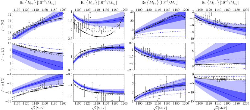
Figure 1: Order-${Q}^{3}$ fits obtained in the heavy baryon approach to the real parts of the $s$- and $p$-wave photoproduction multipoles. The solid, dashed and dotted lines denote the ${Q}^{3}$, ${Q}^{2}$ and ${Q}^{1}$ results, respectively. The darker (lighter) shaded bands show the estimated truncation errors at order ${Q}^{3}$ with $1\sigma$ ($2\sigma$) confidence. The filled circles show the results of the MAID PWA from Ref. Drechsel et al. (2007), the squares (diamonds) are the results of the energy-dependent (independent) SAID analysis from Refs. Briscoe et al. (2019); Strakovsky (Ref. Workman et al. (2012)).

In the $I=3/2$ channel, we find both HB and covariant descriptions satisfactory with the exception of the electric $\Delta$ multipole $E_{1+}^{3/2}$, which is not well reproduced. The latter fact is probably due to the missing $\Delta$ contributions. We expect the description of this amplitude to improve when including them, which will be discussed in section V.4. Note that the shape of the $M_{1+}^{3/2}$ multipole is not well reproduced for CM energies above $\sqrt{s}=$1150\text{\,}\mathrm{MeV}$$, which is also due to missing $\Delta$ dynamics. We expect that the inclusion of the $\Delta$ contributions will correct this behaviour significantly (see also Sec. V.4). The $E_{0+}^{3/2}$ and $M_{1-}^{3/2}$ multipoles are better described in the covariant case, which explains the differences in the fit quality. The smaller value of $\chi^{2}/n$ in the covariant approach may indicate that the Bayesian truncation uncertainties are overestimated or that the fit range is not broad enough to constrain the LECs sufficiently. At this point we emphasize that $n$ should not be equated with the number of degrees of freedom, because our choice of the number of data points is in some way arbitrary. Varying the energy steps results in different values of the reduced $\chi^{2}/n$, therefore one cannot associate a perfect fit with a value of $\chi^{2}/n=1$. The values of $\chi^{2}/n$ should, therefore, not be directly interpreted as a statistical measure of the fit quality but used to compare the relative quality of fits obtained with the same preconditions. Generally, one expects the values of the multipoles at neighboring energy points to be correlated, so that the actual number of degrees of freedom is presumably much smaller than $n$. For this reason, good fits of the empirical data are expected to have $\chi^{2}/n$ considerably smaller than $1$.

In the $I=1/2$ channels, the difference between HB and covariant approach is more pronounced. The descriptions of $E_{0+}^{1/2}$ is clearly better in the covariant approach, and also the description of $M_{1+}^{1/2}$ is better, which is reflected in the fit quality. Clearly, the value of $\chi^{2}/n=1.8$ in the HB case shows that the data cannot be well described. On the other hand, the small value of $\chi^{2}/n=0.2$ obtained in the covariant approach indicates that more data might be required to constrain $d_{9}$ better.

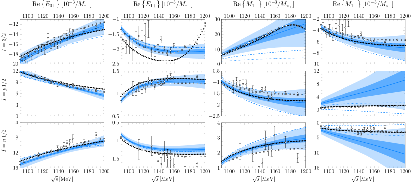
Figure 2: Order-${Q}^{3}$ fits obtained in the covariant approach to the real parts of the $s$- and $p$-wave photoproduction multipoles. The notation is as in Fig. 1.

With the obtained fit values in both approaches, we now analyze the numerical differences between HB and covariant constants as discussed in Sec. V.1. Substituting the employed values of $g_{A}$, $F_{\pi}$ into the right-hand sides of Eq. (52), the numerical values of the predicted shifts read

$$\Delta d_{8}^{\text{IR}}=$0.6\text{\,}{\mathrm{GeV}}^{-2}$, \Delta d_{9}^{\text{IR}}=$0.08\text{\,}{\mathrm{GeV}}^{-2}$,$$

$$\Delta d_{20}^{\text{IR}}=$2.8\text{\,}{\mathrm{GeV}}^{-2}$, \Delta d_{21;22}^{\text{IR}}=$-1.9\text{\,}{\mathrm{GeV}}^{-2}$,$$ (59)

whereas we find for the actual differences from tables 2 and 3

$$\bar{d}_{8}-\hat{d}_{8}^{r}=$2.8\text{\,}{\mathrm{GeV}}^{-2}$, \bar{d}_{9}-\hat{d}_{9}^{r}=$-0.02\text{\,}{\mathrm{GeV}}^{-2}$,$$

$$\bar{d}_{20}-\hat{d}_{20}^{r}=$8.7\text{\,}{\mathrm{GeV}}^{-2}$, \bar{d}_{21;22}-\hat{d}_{21;22}^{r}=$-4.9\text{\,}{\mathrm{GeV}}^{-2}$.$$ (60)

These results show that the IR shifts can, at best, only qualitatively explain the differences between HB and covariant approach. In particular, the agreement for $d_{9}$ is excellent, while for $d_{8}$, $d_{20}$ and $d_{21;22}$, the differences have the same sign as the IR shift. The remaining gap between the two sets of fit parameters is probably due to the poorer fit quality in the HB approach. We also find that the values of the covariant LECs are more natural as in the HB approach. Here, the term “natural” refers to the naive estimate that the $d_{i}$’s should roughly be of order one in the units of $\Lambda_{b}^{-2}$:

$$d_{i}\sim\frac{1}{\Lambda_{b}^{2}}\sim$2.5\text{\,}{\mathrm{GeV}}^{-2}$\mbox{\quad with\quad}\Lambda_{b}=$650\text{\,}\mathrm{MeV}$.$$ (61)

V.4 Order ${Q}^{3}+\epsilon^{2}$ results

In Table 4, we show our fit results for the LECs in the covariant approach at order ${Q}^{3}+\epsilon^{2}$. The reduced $\chi^{2}/n$ is equal to $0.5$ $(1.0)$ in the $I=3/2$ ($I=1/2$) channel.

Table 4: Low-energy constants obtained from an order-${Q}^{3}+\epsilon^{2}$ covariant fit to the real parts of $s$- and $p$-wave photoproduction multipoles of the MAID model from Ref. Drechsel et al. (2007). All LECs are given in units of ${\mathrm{GeV}}^{-2}$, $b_{1}$ is given in $m_{N}^{-1}$.

	$\bar{d}_{8}$	$\bar{d}_{9}$	$\bar{d}_{20}$	$\bar{d}_{21;22}$	$b_{1}$
covariant order-${Q}^{3}+\epsilon^{2}$ fit value:	$0.72(3)$	$0.02(1)$	$-2.1(1)$	$-0.1(1)$	$5.6(1)$

In Fig. 3, we show the results. The most outstanding difference to the $\Delta$-less case is the significantly improved description of the $M_{1+}^{3/2}$ multipole. In comparison to the $\Delta$-less approach, the region beyond $\sqrt{s}=$1150\text{\,}\mathrm{MeV}$$ is reproduced excellently both in magnitude and in shape. The leading $\Delta$ tree diagrams suffice to correct the ${Q}^{3}$ description of $M_{1+}^{3/2}$. However, the description of $E_{1+}^{3/2}$ is unsatisfactory. We presume that including $\epsilon^{3}$ terms will improve the description, because the subleading $\gamma N\Delta$ coupling constant $h_{1}$ contributes at its leading order in $1/m_{N}$ to $E_{1+}^{3/2}$. In the $I=1/2$ channels, for all $s$- and $p$-waves, the data description is not worse than in the $\Delta$-less case. Only $M_{1+}^{1/2}$ was fitted for comparability with the $\Delta$-less approach, all other multipoles are reproduced to a good extent. Here, $M_{1-}^{1/2}$ must be accentuated, which was overshot dramatically in the $\Delta$-less theory.

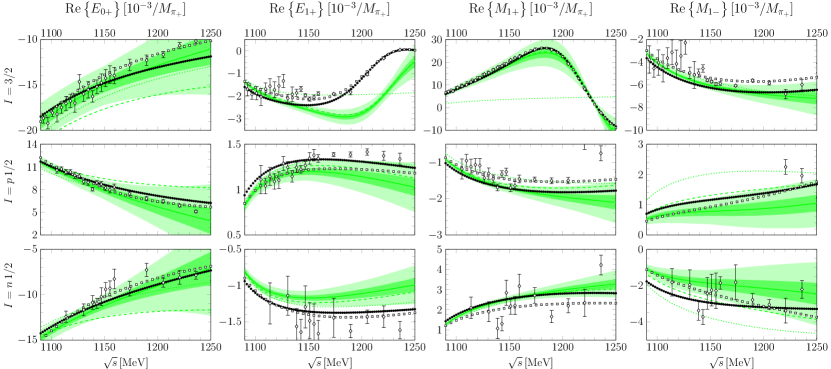
Figure 3: Order-${Q}^{3}+\epsilon^{2}$ fits obtained in the covariant approach to the real parts of the $s$- and $p$-wave photoproduction multipoles. The solid, dashed and dotted lines denote the ${Q}^{3}+\epsilon^{2}$, $\epsilon^{2}$ and $\epsilon^{1}$ results, respectively. The darker (lighter) shaded bands show the estimated truncation errors at order ${Q}^{3}$ with $1\sigma$ ($2\sigma$) confidence. The filled circles show the results of the MAID PWA from Ref. Drechsel et al. (2007), the squares (diamonds) are the results of the energy-dependent (independent) SAID analysis from Refs. Briscoe et al. (2019); Strakovsky (Ref. Workman et al. (2012)).

For the sake of completeness, we mention that we also performed fully comparable fits in the HB approach, using a consistent value of the $\Delta$ mass fitted to the HB order-$\epsilon^{2}$ amplitude of $m_{\Delta}=(1196.1-45.2\,\textup{i})\,$\mathrm{MeV}$.$ In Fig. 4, we show $E_{0+}$ and $M_{1+}$ in the $I=1/2$ channel in order to illustrate that the HB results are, however, by far not as satisfying as the covariant results, which we observe for all multipoles. We conclude that, as expected, the heavy-baryon (non-relativistic) expansion is not quite efficient if one wants to extend the scheme to the $\Delta$ region. Therefore, we do not give the full set of results here, however, we found that the resulting value of $b_{1}=$5.5(1)$m_{N}^{-1}$ is still very close to the covariant one. This is a nice indication of the stability of this constant.

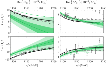
Figure 4: Selected plots of order-${Q}^{3}+\epsilon^{2}$ fits obtained in the heavy baryon approach to the real parts of the $s$- and $p$-wave photoproduction multipoles. The notation is as in Fig. 3.

Next, we take a look at the differences between the $\Delta$-less and -full fit values of the LECs from the point of $\Delta$ resonance saturation, as explained in Sec. V.1. Numerically, the expected differences read, using the covariant fit value of $b_{1}$

$$\delta d_{8}(\Delta)=-\delta d_{21;22}(\Delta)=$-3.4\text{\,}{\mathrm{GeV}}^{-2}$,$$ (62)

and for the actual differences

$$\bar{d}_{8}^{\not{\Delta}}-\bar{d}_{8}^{\Delta}=$-5.6\text{\,}{\mathrm{GeV}}^{-2}$, \bar{d}_{9}^{\not{\Delta}}-\bar{d}_{9}^{\Delta}=$-0.01\text{\,}{\mathrm{GeV}}^{-2}$,$$

$$\bar{d}_{20}^{\not{\Delta}}-\bar{d}_{20}^{\Delta}=$-6.4\text{\,}{\mathrm{GeV}}^{-2}$, \bar{d}_{21;22}^{\not{\Delta}}-\bar{d}_{21;22}^{\Delta}=$9.5\text{\,}{\mathrm{GeV}}^{-2}$.$$ (63)

As one can see, the differences between $\Delta$-less and $\Delta$-full parameters are only very qualitatively explained by the resonance saturation.

In the following, we compare our covariant order-${Q}^{3}+\epsilon^{2}$ results with data of the neutral pion production channel $\gamma p\to\pi^{0}p$. Of the four physical reaction channels given in Eq. (8), this channel is the most interesting for our purposes. The amplitudes for the two charged pion production channels $\gamma p\to\pi^{+}n$ and $\gamma n\to\pi^{-}p$ are dominated by the leading order Kroll-Ruderman terms, such that subleading terms give only very small corrections. The remaining neutral channel $\gamma n\to\pi^{0}n$ is difficult to measure in experiments since this requires a neutron target. Therefore, little data are available for this channel.

The recent experiment at the Mainz Microtron (MAMI) provided high-precision data for the differential cross section $\derivative{\sigma}{\Omega}$ and the linearly polarized photon asymmetry $\Sigma$ Hornidge et al. (2013); Hornidge (2013, ). We compare our findings with these data and emphasize that our results for both observables were calculated as discussed in Sec. II, in particular we do not use the $s$- and $p$-wave approximation. In Figs. 5 and 6, we depict our results obtained from the covariant order-${Q}^{3}+\epsilon^{2}$ fit, where the depicted error bars show the combined statistical and systematic error

$$\delta O_{i}=\sqrt{\left(\delta O_{i}^{\text{stat}}\right)^{2}+\left(\delta O_{i}^{\text{sys}}\right)^{2}}.$$ (64)

The systematic uncertainties are $4\text{\,}\mathrm{\char 37\relax}$ for $\derivative{\sigma}{\Omega}$ and $5\text{\,}\mathrm{\char 37\relax}$ for $\Sigma$.

In the analysis of the $s$- and $p$-wave multipole amplitudes, we found that the order-${Q}^{3}+\epsilon^{2}$ covariant fits give an overall accurate reproduction in our considered energy region. By comparison with the differential cross section and polarization asymmetry, we find our observation confirmed. Especially the polarization asymmetries are reproduced accurately up to the $\Delta$ region.

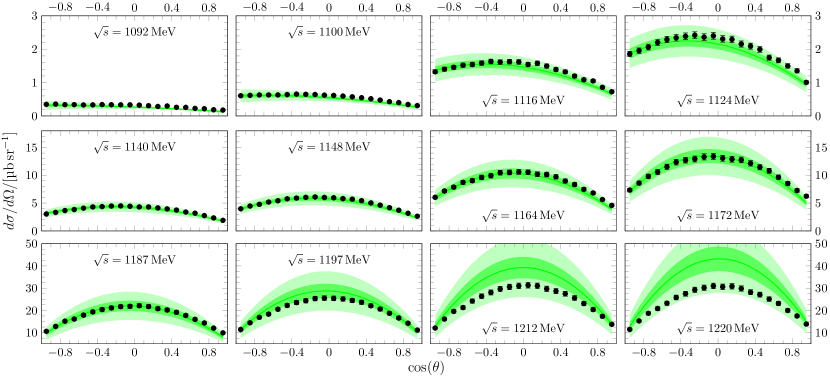
Figure 5: Covariant order-${Q}^{3}+\epsilon^{2}$ result of the unpolarized differential cross section in the channel $\gamma+p\to\pi^{0}+p$. The solid lines denote the ${Q}^{3}+\epsilon^{2}$ results, the darker (lighter) shaded bands show the estimated truncation errors at order ${Q}^{3}+\epsilon^{2}$ with $1\sigma$ ($2\sigma$) confidence. The data are from Refs. Hornidge et al. (2013); Hornidge , error bars correspond to the combined statistical and systematical error.

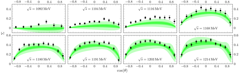
Figure 6: Covariant order-${Q}^{3}+\epsilon^{2}$ result of the linearly polarized photon asymmetry in the channel $\gamma+p\to\pi^{0}+p$. The solid lines denote the ${Q}^{3}+\epsilon^{2}$ results, the darker (lighter) shaded bands show the estimated truncation errors at order ${Q}^{3}+\epsilon^{2}$ with $1\sigma$ ($2\sigma$) confidence. The data are from Refs. Hornidge et al. (2013); Hornidge (2013, ), error bars correspond to the combined statistical and systematical error.

V.5 Order $\epsilon^{3}$ results

Finally, we give our results for the LECs determined from the covariant fit at order $\epsilon^{3}$ in Table 5. In the $I=3/2$ fit, the number of used data points is $204$ due to the inclusion of the $E_{1+}$ multipole and $102$ in the $I=1/2$ channel. The reduced $\chi^{2}/n$ is equal to $0.2(2.2)$ in the $I=3/2$($I=1/2$) channel. The corresponding results for the multipoles are depicted in Fig. 7.

Table 5: Low-energy constants obtained from an order-$\epsilon^{3}$ covariant fit to the real parts of $s$- and $p$-wave photoproduction multipoles of the MAID model from Ref. Drechsel et al. (2007). All LECs are given in units of ${\mathrm{GeV}}^{-2}$, $\bar{b}_{1}$ and $\bar{h}_{1}$ are given in $m_{N}^{-1}$.

	$\bar{d}_{8}$	$\bar{d}_{9}$	$\bar{d}_{20}$	$\bar{d}_{21;22}$	$\bar{b}_{1}$	$\bar{h}_{1}$
covariant order-$\epsilon^{3}$ fit value:	$-0.25(4)$	$-0.73(2)$	$2.2(1)$	$-6.8(1)$	$5.3(1)$	$0.9(1)$

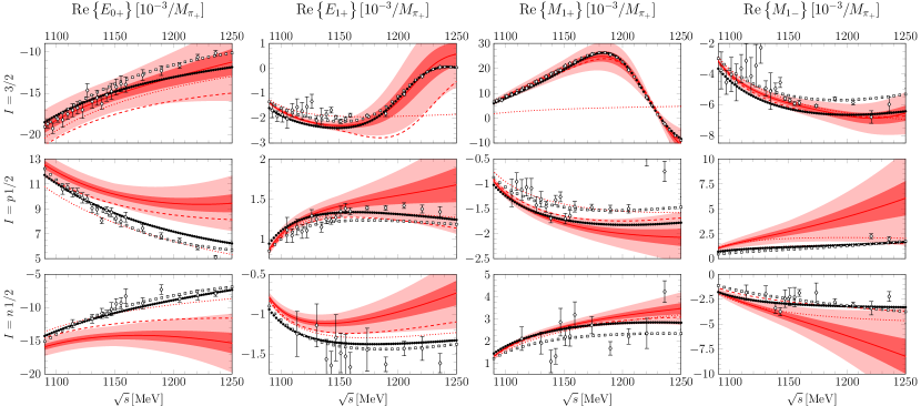
Figure 7: Order-$\epsilon^{3}$ fits obtained in the covariant approach to the real parts of the $s$- and $p$-wave photoproduction multipoles. The solid, dashed and dotted lines denote the $\epsilon^{3},\epsilon^{2}$ and $\epsilon^{1}$ results, respectively. The darker (lighter) shaded bands show the estimated truncation errors at order ${Q}^{3}$ with $1\sigma$ ($2\sigma$) confidence. The filled circles show the results of the MAID PWA from Ref. Drechsel et al. (2007), the squares (diamonds) are the results of the energy-dependent (independent) SAID analysis from Refs. Briscoe et al. (2019); Strakovsky (Ref. Workman et al. (2012)).

As we can see from Fig. 7, the reproduction of the $I=3/2$ channel has improved compared to the covariant ${Q}^{3}+\epsilon^{2}$ fit. Especially $E_{1+}$ is now matched significantly better due to the inclusion of the subleading $\gamma N\Delta$ coupling constant $\bar{h}_{1}$. In the $I=1/2$ channels however, the description is distinctly worse compared to the ${Q}^{3}+\epsilon^{2}$-case. Especially the reproduction of the $E_{0+}^{1/2}$ multipoles fails, which has a substantial effect on the reproduction of cross sections, for example. Also, the fit quality in the $I=1/2$ channels of $\chi^{2}/n=2.2$ is significantly worse compared to the ${Q}^{3}+\epsilon^{2}$ fit, where we found $\chi^{2}/n=1.0$. We also remark that $M_{1-}^{1/2}$ is overshot again, but not as badly as in the $\Delta$-less case (see Fig. 2). These observations indicate a slow convergence of the scheme in the $I=1/2$ channels, and one needs to extend the calculation to higher orders (such as ${Q}^{4}+\epsilon^{3}$ or $\epsilon^{4}$) to obtain a better description of the data.

In order to check that our determined value of the $\Delta$ mass in the covariant scheme is consistent with the $\Delta$ contribution to the $\pi N$ elastic channel, we plot the imaginary part of $E_{1+}^{3/2}$ and $M_{1+}^{3/2}$ in Fig. 8. Because the phase of the pion photoproduction amplitude is determined by the elastic $\pi N$ phase shifts, a satisfying reproduction of the imaginary parts is important. We find the agreement reasonable, with the deviation in $\imaginary\{M_{1+}^{3/2}\big{\}}$ close to threshold originating from the usage of the constant imaginary part of the $\Delta$ mass in the $\Delta$ pole diagrams. Furthermore, the $E2/M1$ ratio

$$R_{EM}=\frac{\imaginary\{E_{1+}^{3/2}\big{\}}}{\imaginary\{M_{1+}^{3/2}\big{\}}}\Bigg{|}_{\sqrt{s}=$1232\text{\,}\mathrm{MeV}$}\approx-0.033\pm 0.014$$ (65)

is consistent with the PDG value $-0.030\lesssim R_{EM}\lesssim-0.020$ Zyla et al. (2020), whereas at order ${Q}^{3}+\epsilon^{2}$, we found $R_{EM}\approx-0.071\pm 0.014$.

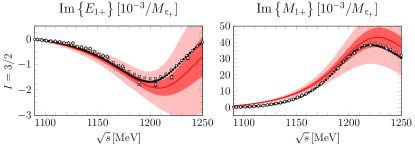
Figure 8: Imaginary parts of $E_{1+}^{3/2}$ and $M_{1+}^{3/2}$ using the covariant order-$\epsilon^{3}$ fit results. The notation is as in Fig. 7.

VI Summary and conclusions

We have studied pion photoproduction in chiral effective field theory with explicit $\Delta$ degrees of freedom. Starting from the $\Delta$-less approach, we considered the reaction up to the leading loop order in the heavy baryon and in the manifestly covariant schemes. In particular, we analyzed the difference between the obtained HB and covariant results for low-energy constants in terms of the infrared regular shifts. We extended our calculations to the leading $\Delta$ contributions employing the complex-mass approach using a fitted $\Delta$ mass and studied the effects of resonance saturation to the LECs. Moreover, we for the first time provide results for pion photoproduction at order $\epsilon^{3}$ in the small scale expansion scheme, where the leading $\Delta$-full loop order is taken into account. The results for the LECs $\bar{d}_{8},\bar{d}_{9},\bar{d}_{20},\bar{d}_{21;22},\bar{b}_{1}$ and $\bar{h}_{1}$ are obtained by fits to the MAID partial-wave analysis using a Bayesian approach to theoretical uncertainties.

The main conclusions of our analysis of pion photoproduction can be summarized as follows:

• In the $\Delta$-less approach, the description of pion photoproduction is satisfying only in a very limited energy range above threshold and fails approaching the $\Delta$ region. Especially for the magnetic multipole $M_{1+}^{3/2}$, the description agrees with the data only up to approximately $\sqrt{s}=$1150\text{\,}\mathrm{MeV}$$. Studying the reaction in the covariant framework yields a better agreement with the data than the heavy baryon approach. The results of our calculations are very relevant for ongoing investigations of few-nucleon electromagnetic reactions, see Ref. Krebs (2020) for a review article. While the two-nucleon charge density operator at the leading one-loop order does not involve LECs from $\mathcal{L}_{\pi N}^{(3)}$ Kölling et al. (2009, 2011), which allowed us to perform high-accuracy calculation of the deuteron charge and quadrupole form factors Filin et al. (2020, 2021), the corresponding current operator depends on the LECs $d_{8}$, $d_{9}$, $d_{21}$ and $d_{22}$ Kölling et al. (2011). In particular, the LEC $d_{9}$ governs the long-range two-nucleon contribution to the deuteron magnetic form factor Kölling et al. (2012).

• Incorporating the leading $\Delta$ tree contributions significantly extends the energy range in which a good agreement with the $s$- and $p$-wave multipoles can be achieved. We found that the leading $\gamma N\Delta$ coupling constant $b_{1}$ is stable with respect to variation of the energy range, assigned relative error to the data and combination of $I=3/2$ and $I=1/2$ fit. The difference between the numerical values of the LECs obtained in a $\Delta$-less and $\Delta$-full approach can, at least very qualitatively, be explained in terms of resonance saturation. The results from the covariant order-${Q}^{3}+\epsilon^{2}$ calculation are found to reproduce the high-precision data of cross sections and polarization asymmetries from Refs. Hornidge et al. (2013); Hornidge (2013, ) remarkably well. On the other hand, the order-${Q}^{3}+\epsilon^{2}$ calculation performed within the heavy baryon scheme demonstrates a much worse description of the data. This is an indication of the fact that the $1/m_{N}$ expansion is not efficient in the $\Delta$ region.

• The next-to-leading $\Delta$ contributions give rise to surprisingly large corrections to the scattering amplitude. However, these corrections are important to achieve a reasonable description of $E_{1+}^{3/2}$. At the same time, the description of the $I=1/2$ channel gets worsened significantly. The overall reproduction of the $s$- and $p$-wave multipoles is worse than in the ${Q}^{3}+\epsilon^{2}$ approach. However, the given estimate of the leading and subleading $\gamma N\Delta$ coupling constants $b_{1}$ and $h_{1}$ can be taken as reliable, because the isospin-$3/2$ channel is very well described. Also, the values agree with our findings from Ref. Rijneveen et al. (2021). Notice further that while the explicit treatment of the $\Delta$-resonance in $\chi$PT helps to avoid the unnecessary lowering of the breakdown scale $\Lambda_{b}$, the expansion parameter in the $\Delta$-scheme becomes $\propto\Delta$. It is, therefore, not a priori clear that the framework with explicit $\Delta$ degrees of freedom features a smaller expansion parameter. For example, the $1/m_{N}$-expansion of the nucleon polarizabilities was found to converge considerably slower upon the explicit inclusion of the $\Delta$-resonance Thürmann et al. (2021). Thus, the most efficient scheme can only be determined upon performing explicit calculations.

Based on the conclusions of our analysis of pion photoproduction, we find that it would be very interesting to extend the analysis in the following points. In our work, we have focused on calculating the $s$- and $p$-wave multipoles, because they give by far the largest contributions to cross sections. However, in Refs. Fernandez-Ramirez et al. (2009a, b), the importance of $d$-waves to observables was pointed out. Therefore, it would be worthwhile to extend the analysis to higher partial waves or to the analysis of observables directly. Also, further insight could be gained from extending the covariant analysis to higher orders (${Q}^{4}+\epsilon^{3}$ or $\epsilon^{4}$) given the fairly slow convergence of the small scale expansion scheme. A $\Delta$-less ${Q}^{4}$ calculation was already provided by Hilt et al. Hilt et al. (2013a), but the improvement in the description was only moderate, especially in the $\Delta$ region. Since our analysis revealed significant improvement in the description of $I=3/2$ multipole amplitudes in the $\Delta$ region, but a worse description of the $I=1/2$ channels, the effects of the ${Q}^{4}$ ($\epsilon^{4}$) terms in combination with the order-$\epsilon^{3}$ terms would be most interesting to study.

Appendix A Relating different sets of amplitudes

The relation between the coefficients $A_{i}$ and $B_{i}$ of Eq. (11) and Eq. (14) can be found by equating the two representations:

$$\sum_{i=1}^{8}B_{i}V_{i}^{\mu}=\sum_{i=1}^{4}A_{i}\mathcal{M}_{i}^{\mu}.$$ (66)

Remembering that $V_{4}$ and $V_{8}$ are not needed for real photons ($\epsilon\cdot k=0,k^{2}=0$) and using the two relations obtained by current conservation of the matrix element (13), the coefficients $A_{i}$ can be obtained from $B_{i}$ as follows:

$$A_{1}=\textup{i}(B_{5}+m_{N}B_{6}),\quad A_{2}=\textup{i}\frac{B_{3}}{k\cdot p+k\cdot p^{\prime}},\quad A_{3}=\textup{i}B_{7},\quad A_{4}=\frac{\textup{i}}{2}B_{6}.$$ (67)

The relations between the invariant amplitudes $A_{i}$ and the amplitudes $\mathcal{F}_{i}$ read:

$$\mathcal{F}_{1} =-\frac{W-m_{N}}{8\uppi W}\sqrt{(E_{p}+m_{N})(E_{p^{\prime}}+m_{N})}\left[A_{1}+(W-m_{N})A_{4}-\frac{2\nu}{W-m_{N}}(A_{3}-A_{4})\right],$$

$$\mathcal{F}_{2} =-\frac{W+m_{N}}{8\uppi W}\,\absolutevalue{\boldsymbol{q}}\,\sqrt{\frac{E_{p}-m_{N}}{E_{p^{\prime}}+m_{N}}}\left[-A_{1}+(W+m_{N})A_{4}-\frac{2\nu}{W+m_{N}}(A_{3}-A_{4})\right],$$

$$\mathcal{F}_{3} =-\frac{W+m_{N}}{8\uppi W}\,\absolutevalue{\boldsymbol{q}}\,\sqrt{(E_{p}-m_{N})(E_{p^{\prime}}+m_{N})}\left[\frac{W^{2}-m_{N}^{2}}{W+m_{N}}A_{2}+A_{3}-A_{4}\right],$$

$$\mathcal{F}_{4} =-\frac{W-m_{N}}{8\uppi W}\,\absolutevalue{\boldsymbol{q}}^{2}\,\sqrt{\frac{E_{p}+m_{N}}{E_{p^{\prime}}+m_{N}}}\left[-\frac{W^{2}-m_{N}^{2}}{W-m_{N}}A_{2}+A_{3}-A_{4}\right],$$ (68)

where we have used $\nu=-\tfrac{1}{2}k\cdot q$ and $W=\sqrt{s}$ is the CM energy.

Appendix B Feynman diagrams

In Figs. 9, 10, 11, 12 and 13, we present the Feynman diagrams for pion photoproduction, which appear at order $\epsilon^{3}$. We cluster them in five gauge-invariant sets. The lower-order diagrams were already shown in Ref. Rijneveen et al. (2021).

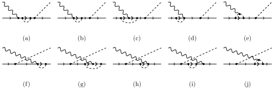
Figure 9: First set of $\Delta$-full loop diagrams.

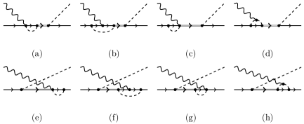
Figure 10: Second set of $\Delta$-full loop diagrams.

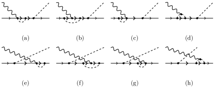
Figure 11: Third set of $\Delta$-full loop diagrams.

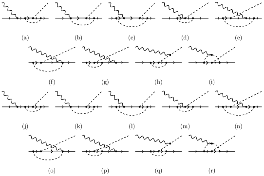
Figure 12: Fourth set of $\Delta$-full loop diagrams.

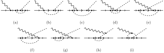
Figure 13: Fifth set of $\Delta$-full loop diagrams.

Appendix C Counter terms

In this Appendix, we present the expressions for the renormalized quantities and the counter terms.

C.1 Loop integrals

The loop integral functions are defined as

$$A_{0}(m^{2}) =\frac{1}{\textup{i}}\int\frac{\differential^{d}l}{(2\uppi)^{d}}\frac{\mu^{4-d}}{l^{2}-m^{2}},$$

$$B_{0}(p^{2},m_{0}^{2},m_{1}^{2}) =\frac{1}{\textup{i}}\int\frac{\differential^{d}l}{(2\uppi)^{d}}\frac{\mu^{4-d}}{(l^{2}-m_{0}^{2})((l+p)^{2}-m_{1}^{2})},$$

$$J_{0}(\omega) =\frac{1}{\textup{i}}\int\frac{\differential^{d}l}{(2\uppi)^{d}}\frac{\mu^{4-d}}{(l^{2}-M_{\pi}^{2})(v\cdot l+\omega)},$$

$$C_{0}(p^{2},(p-q)^{2},q^{2},m_{0}^{2},m_{1}^{2},m_{2}^{2}) =\frac{1}{\textup{i}}\int\frac{\differential^{d}l}{(2\uppi)^{d}}\frac{\mu^{4-d}}{(l^{2}-m_{0}^{2})((l+p)^{2}-m_{1}^{2})((l+q)^{2}-m_{2}^{2})}.$$ (69)

C.2 Mesonic counter terms

The renormalization rules for the pion mass, field redefinition and decay constant are given below. We remind that the parameter $\upalpha$ is the unphysical constant from the general pion field parametrization (Eq. (23)).

$$M^{2}= \,M_{\pi}^{2}+\delta M^{(4)}, \delta M^{(4)}= \,\frac{M_{\pi}^{2}}{2F_{\pi}^{2}}(A_{0}(M_{\pi}^{2})-4M_{\pi}^{2}\,l_{3}),$$ (70)

$$Z_{\pi}= \,1+\delta Z_{\pi}^{(4)}, \delta Z_{\pi}^{(4)}= \,\frac{1}{F_{\pi}^{2}}(A_{0}(M_{\pi}^{2})(1-10\upalpha)-2M_{\pi}^{2}\,l_{4}),$$ (71)

$$F= \,F_{\pi}+\delta F_{\pi}^{(4)}, \delta F_{\pi}^{(4)}= -\frac{1}{F_{\pi}}(A_{0}(M_{\pi}^{2})+M_{\pi}^{2}\,l_{4}).$$ (72)

C.3 Heavy baryon counter terms

Nucleon mass and field renormalization

The HB expressions for the redefinition of the nucleon mass and field read

$$m =m_{N}+\delta m^{(2)}+\delta m^{(3)}, \delta m^{(2)} =4c_{1}M_{\pi}^{2}, \delta m^{(3)} =-\frac{3g_{A}^{2}M_{\pi}^{2}}{4F_{\pi}^{2}}J_{0}(0),$$ (73)

$$Z_{N} =1+\delta Z_{N}^{(3)}, \delta Z_{N}^{(3)} =-\frac{3g_{A}^{2}M_{\pi}^{2}}{32\,\uppi^{2}F_{\pi}^{2}}+\frac{9g_{A}^{2}}{4F_{\pi}^{2}}A_{0}(M_{\pi}^{2}).$$ (74)

$\Delta$ mass and field renormalization.

The $\Delta$ mass and field are renormalized as

$$\mathring{m}_{\Delta} =m_{\Delta}+\text{\leavevmode{d}}m_{\Delta}^{(2)}+\dots\,,\quad\quad\text{\leavevmode{d}}m_{\Delta}^{(2)}=4c_{1}^{\Delta}M_{\pi}^{2}\,,$$ (75)

and

$$Z_{\Delta} =1+\dots\,,$$ (76)

where the ellipses refer to terms which are not relevant at the considered order in the expansion.

Axial nucleon coupling

The renormalization rules for the axial nucleon coupling constant $g_{A}$ in the HB sector are given below. Note that we already taken into account the Goldberger-Treiman discrepancy to fully remove the redundant for pion photoproduction constant $d_{18}$ from the rules. For a recent high-precision determination of the pion-nucleon coupling constants and the Goldberger-Treiman discrepancy from neutron-proton and proton-proton scattering data see Ref. Reinert et al. (2021). Here, $g$ is the bare, $g_{A}$ is the physical constant.

$$g=g_{A}+\delta g^{(3)},\quad\delta g^{(3)}=\left(-4d_{16}+2d_{18}+\frac{g_{A}^{3}}{16\,\uppi^{2}F_{\pi}^{2}}\right)M_{\pi}^{2}-\frac{(g_{A}+2g_{A}^{3})}{F_{\pi}^{2}}A_{0}(M_{\pi}^{2}).$$ (77)

Electromagnetic form factors of the nucleon

The replacement rules for the counter terms of the constants $c_{6}$ and $c_{7}$ are given below, where we denote the renormalized quantities by the bar.

$$c_{6} =\bar{c}_{6}+\delta c_{6}^{(3)}, \delta c_{6}^{(3)} =-\frac{2m_{N}g_{A}^{2}}{F_{\pi}^{2}}J_{0}(0),$$ (78)

$$c_{7} =\bar{c}_{7}+\delta c_{7}^{(3)}, \delta c_{7}^{(3)} =\frac{m_{N}g_{A}^{2}}{F_{\pi}^{2}}J_{0}(0).$$ (79)

C.4 Covariant counter terms

Nucleon mass and field renormalization

In the following, we introduce the dimensionless parameters $\alpha=\frac{M_{\pi}}{m_{N}}$ and $\beta=\frac{m_{\Delta}}{m_{N}}$. The ratio of the masses $\alpha$ is not to be confused with the unphysical off-shell parameter $\upalpha$. The renormalization rules for the nucleon mass and field redefinition are given below. For convenience, we give the contributions arising from the $\Delta$ resonance separately. This means that all corrections $\delta x^{(i,\Delta)}$ are set to zero in the $\Delta$-less case.

$$m =m_{N}+\delta m_{N}^{(2)}+\delta m_{N}^{(3)}+\delta m_{N}^{(3,\Delta)},$$ (80)

$$\delta m_{N}^{(2)} =4M_{\pi}^{2}\,c_{1},$$ (81)

$$\delta m_{N}^{(3)} =-\frac{3g_{A}^{2}m_{N}}{2F_{\pi}^{2}}(A_{0}(m_{N}^{2})+M_{\pi}^{2}B_{0}(m_{N}^{2},M_{\pi}^{2},m_{N}^{2})),$$ (82)

$$\delta m_{N}^{(3,\Delta)} =-\frac{h_{A}^{2}m_{N}^{3}}{576\,\uppi^{2}F_{\pi}^{2}\beta^{2}}\left[\alpha^{4}(16\beta+13)-4\alpha^{2}(3\beta+2)+3\beta^{4}-12\beta^{3}-4\beta^{2}+4\beta+2\right]$$

$$+\frac{m_{N}h_{A}^{2}}{6F_{\pi}^{2}\beta^{2}}\Big{[}\left(\alpha^{4}-\alpha^{2}\left(2\beta^{2}-6\beta-5\right)+(\beta-1)(\beta+1)^{3}\right)A_{0}(M_{\pi}^{2})$$

$$\qquad\qquad-\left(\alpha^{4}-2\alpha^{2}\left(\beta^{2}+\beta+1\right)+\beta^{4}+2\beta^{3}-\beta^{2}+2\beta+1\right)A_{0}(m_{\Delta}^{2})$$

$$\qquad\qquad-\left(\alpha^{2}-(\beta-1)^{2}\right)\left(\alpha^{2}-(\beta+1)^{2}\right)^{2}m_{N}^{2}\,B_{0}(m_{N}^{2},M_{\pi}^{2},m_{\Delta}^{2})\Big{]},$$ (83)

$$Z_{N} =1+\delta Z_{N}^{(3)}+\delta Z_{N}^{(3,\Delta)},$$ (84)

$$\delta Z_{N}^{(3)} =\frac{3g_{A}^{2}}{4F_{\pi}^{2}(\alpha^{2}-4)}\Big{[}\frac{M_{\pi}^{2}}{4\uppi^{2}}+(5\alpha^{2}-12)A_{0}(M_{\pi}^{2})-4\alpha^{2}A_{0}(m_{N}^{2})-4M_{\pi}^{2}(\alpha^{2}-3)B_{0}(m_{N}^{2},M_{\pi}^{2},m_{N}^{2})\Big{]},$$ (85)

$$\delta Z_{N}^{(3,\Delta)} =\frac{h_{A}^{2}}{6F_{\pi}^{2}\beta^{2}}\Big{[}\left(3\alpha^{4}-\alpha^{2}\left(6\beta^{2}+4\beta+9\right)+(\beta+1)^{2}(3\beta^{2}-2\beta+5)\right)A_{0}(M_{\pi}^{2})$$

$$\quad\quad-\left(3\alpha^{4}+\alpha^{2}(-6\beta^{2}-4\beta+2)+3\beta^{4}+4\beta^{3}+\beta^{2}-8\beta-5\right)A_{0}(m_{\Delta}^{2})$$

$$\quad\quad-\Big{(}3\alpha^{6}-\alpha^{4}(9\beta^{2}+4\beta+1)-\alpha^{2}(-9\beta^{4}-8\beta^{3}-2\beta^{2}+4\beta+7)$$

$$\quad\quad-(\beta+1)^{3}(3\beta^{3}-5\beta^{2}+7\beta-5)\Big{)}m_{N}^{2}\,B_{0}(m_{N}^{2},M_{\pi}^{2},m_{\Delta}^{2})\Big{]}.$$ (86)

$\Delta$ mass and field renormalization.

The $\Delta$ mass and field are renormalized as

$$\mathring{m}_{\Delta} =m_{\Delta}+\text{\leavevmode{d}}m_{\Delta}^{(2)}+\dots\,,\quad\quad\text{\leavevmode{d}}m_{\Delta}^{(2)}=4c_{1}^{\Delta}M_{\pi}^{2}\,,$$ (87)

and

$$Z_{\Delta} =1+\dots\,.$$ (88)

where the ellipses refer to terms which are not relevant at the considered order in the expansion.

Axial nucleon coupling

The renormalization rules for the axial nucleon coupling constant $g_{A}$ are given below. Note that we use the auxiliary variables $a_{i},b_{i},c_{i}$ only in this particular context for reasons of clarity and comprehensibility.

$$g =\,g_{A}+\delta g^{(3)}+\delta g^{(3,\Delta)},$$ (89)

$$\delta g^{(3)} =-2(2d_{16}-d_{18})M_{\pi}^{2}-\frac{3g_{A}^{3}M_{\pi}^{2}}{16\uppi^{2}F_{\pi}^{2}(\alpha^{2}-4)}-\frac{g_{A}}{F_{\pi}^{2}(\alpha^{2}-4)}\Big{[}(\alpha^{2}-4+2g_{A}^{2}(2\alpha^{2}-5))A_{0}(M_{\pi}^{2})$$

$$\qquad\quad+(8-(2+3g_{A}^{2})\alpha^{2})A_{0}(m_{N}^{2})+g_{A}^{2}m_{N}^{2}(\alpha^{2}-4)B_{0}(M_{\pi}^{2},m_{N}^{2},m_{N}^{2})$$

$$\qquad\quad+(8-2\alpha^{2}-3g_{A}^{2}(\alpha^{2}-3))M_{\pi}^{2}\,B_{0}(m_{N}^{2},M_{\pi}^{2},m_{N}^{2})+g_{A}^{2}M_{\pi}^{2}m_{N}^{2}(\alpha^{2}-4)C_{0}(m_{N}^{2},M_{\pi}^{2},m_{N}^{2},M_{\pi}^{2},m_{N}^{2},m_{N}^{2})\Big{]},$$ (90)

$$\delta g^{(3,\Delta)} =a_{0}+a_{1}A_{0}(M_{\pi}^{2})+a_{2}A_{0}(m_{N}^{2})+a_{3}A_{0}(m_{\Delta}^{2})+b_{1}B_{0}(M_{\pi}^{2},m_{N}^{2},m_{\Delta}^{2})+b_{2}B_{0}(M_{\pi}^{2},m_{\Delta}^{2},m_{\Delta}^{2})$$

$$+b_{3}B_{0}(m_{N}^{2},M_{\pi}^{2},m_{N}^{2})+b_{4}B_{0}(m_{N}^{2},M_{\pi}^{2},m_{\Delta}^{2})+c_{1}C_{0}(m_{N}^{2},M_{\pi}^{2},m_{N}^{2},M_{\pi}^{2},m_{N}^{2},m_{\Delta}^{2})$$

$$+c_{2}C_{0}(m_{N}^{2},M_{\pi}^{2},m_{N}^{2},M_{\pi}^{2},m_{\Delta}^{2},m_{\Delta}^{2}),$$ (91)

$$a_{0} =-\frac{g_{A}h_{A}^{2}m_{N}^{2}}{5184\,\uppi^{2}F_{\pi}^{2}\beta^{2}}\Big{[}\alpha^{4}(24\beta+325)-4\alpha^{2}\left(3\beta^{4}-6\beta^{3}-8\beta^{2}+140\beta+45\right)+12\alpha^{6}-69\beta^{4}-384\beta^{3}+100\beta^{2}$$

$$\qquad\quad+248\beta+158\Big{]}$$

$$-\frac{5g_{1}h_{A}^{2}m_{N}^{2}}{31104\,\uppi^{2}F_{\pi}^{2}\beta^{4}}\Big{[}3\alpha^{10}-\alpha^{8}\left(3\beta^{2}+5\beta+9\right)-\alpha^{6}\left(3\beta^{4}-10\beta^{2}-30\beta+60\right)$$

$$\qquad\quad+\alpha^{4}\left(3\beta^{6}+5\beta^{5}-3\beta^{4}-20\beta^{3}-114\beta^{2}-248\beta-34\right)$$

$$\qquad\quad-2\alpha^{2}\left(7\beta^{6}+59\beta^{5}-129\beta^{4}-59\beta^{3}-76\beta^{2}-68\beta-2\right)$$

$$\qquad\quad-2\beta\left(17\beta^{5}-82\beta^{4}+18\beta^{3}+28\beta^{2}+42\beta+20\right)\Big{]},$$ (92)

$$a_{1} =\,-\frac{g_{A}h_{A}^{2}}{54F_{\pi}^{2}\beta^{2}}\Big{[}4\alpha^{6}+\alpha^{4}\left(-8\beta^{2}-8\beta+31\right)+\alpha^{2}\left(4\beta^{4}+8\beta^{3}-46\beta^{2}-69\right)+23\beta^{4}+4\beta^{3}+12\beta^{2}+56\beta+25\Big{]}$$

$$+\frac{5g_{1}h_{A}^{2}}{972F_{\pi}^{2}\beta^{4}}\Big{[}3\alpha^{10}-\alpha^{8}\left(9\beta^{2}+5\beta+10\right)+\alpha^{6}\left(9\beta^{4}+10\beta^{3}+23\beta^{2}+17\beta+6\right)$$

$$\qquad\quad-\alpha^{4}\left(3\beta^{6}+5\beta^{5}+27\beta^{4}+36\beta^{3}+55\beta^{2}+33\beta-35\right)$$

$$\qquad\quad+2\alpha^{2}\left(7\beta^{6}+17\beta^{5}+17\beta^{4}-14\beta^{3}+44\beta^{2}+71\beta+21\right)-2(\beta+1)^{2}\left(7\beta^{4}-4\beta^{3}-9\beta^{2}+10\beta+2\right)\Big{]},$$ (93)

$$a_{2} =\frac{2g_{A}h_{A}^{2}}{27F_{\pi}^{2}\alpha^{2}\beta^{2}}\Big{[}5\alpha^{6}+3\alpha^{4}(2\beta+9)+\alpha^{2}\left(-3\beta^{3}-6\beta^{2}+33\beta+16\right)+6(\beta-1)(\beta+1)^{2}\Big{]},$$ (94)

$$a_{3} =\frac{g_{A}h_{A}^{2}}{54F_{\pi}^{2}\alpha^{2}\beta^{2}}\Big{[}4\alpha^{8}+\alpha^{6}\left(-8\beta^{2}-8\beta+15\right)+\alpha^{4}\left(4\beta^{4}+8\beta^{3}-50\beta^{2}-8\beta+30\right)$$

$$\qquad\quad+\alpha^{2}\left(23\beta^{4}+16\beta^{3}+13\beta^{2}-92\beta-73\right)-24(\beta-1)(\beta+1)^{2}\Big{]}$$

$$+\frac{5g_{1}h_{A}^{2}}{972F_{\pi}^{2}\beta^{4}}\Big{[}3\alpha^{10}-\alpha^{8}\left(9\beta^{2}+5\beta+7\right)+\alpha^{6}\left(9\beta^{4}+10\beta^{3}+17\beta^{2}+12\beta-1\right)$$

$$\qquad\quad-\alpha^{4}\left(3\beta^{6}+5\beta^{5}+24\beta^{4}+31\beta^{3}+42\beta^{2}-15\beta-15\right)$$

$$\qquad\quad+2\alpha^{2}\left(7\beta^{6}+17\beta^{5}+10\beta^{4}-5\beta^{3}+18\beta^{2}-25\beta-7\right)-14\beta^{6}-20\beta^{5}+34\beta^{4}-20\beta^{3}+22\beta^{2}+28\beta+4\Big{]},$$ (95)

$$b_{1} =\frac{2g_{A}h_{A}^{2}m_{N}^{2}}{9F_{\pi}^{2}\alpha^{2}\beta^{2}}\Big{[}\alpha^{6}+\alpha^{4}\beta(7\beta+3)+\alpha^{2}\left(-2\beta^{4}+\beta^{3}+\beta^{2}-5\beta-3\right)+2(\beta-1)^{2}(\beta+1)^{3}\Big{]},$$ (96)

$$b_{2} =-\frac{5g_{1}h_{A}^{2}m_{N}^{2}}{486F_{\pi}^{2}\beta^{3}}\Big{[}5\alpha^{6}+\alpha^{4}\left(8\beta^{2}-6\beta-11\right)-2\alpha^{2}\left(8\beta^{4}+18\beta^{3}+13\beta^{2}-6\beta-3\right)$$

$$\qquad\quad+4\beta^{2}\left(3\beta^{4}+6\beta^{3}-2\beta^{2}+6\beta+3\right)\Big{]},$$ (97)

$$b_{3} =\frac{2g_{A}h_{A}^{2}m_{N}^{2}}{27F_{\pi}^{2}\alpha^{2}\beta^{2}}\Big{[}5\alpha^{8}+2\alpha^{6}(3\beta+7)+\alpha^{4}\left(-3\beta^{3}-12\beta^{2}+24\beta+5\right)$$

$$\qquad\quad+12\alpha^{2}(\beta-1)(\beta+1)^{2}-6\left(\beta^{5}-\beta^{3}+\beta^{2}-1\right)\Big{]},$$ (98)

$$b_{4} =\frac{g_{A}h_{A}^{2}m_{N}^{2}}{54F_{\pi}^{2}\alpha^{2}\beta^{2}}\Big{[}4\alpha^{10}+\alpha^{8}\left(-12\beta^{2}-8\beta+11\right)+\alpha^{6}\left(12\beta^{4}+16\beta^{3}-61\beta^{2}+3\right)$$

$$\qquad\quad+\alpha^{4}\left(-4\beta^{6}-8\beta^{5}+73\beta^{4}+48\beta^{3}+2\beta^{2}-96\beta-79\right)-\alpha^{2}(\beta+1)^{2}\left(23\beta^{4}-30\beta^{3}+26\beta^{2}+66\beta-85\right)$$

$$\qquad\quad+24\left(\beta^{5}-\beta^{3}+\beta^{2}-1\right)\Big{]}$$

$$+\frac{5g_{1}h_{A}^{2}m_{N}^{2}}{972F_{\pi}^{2}\beta^{4}}\Big{[}3\alpha^{12}-\alpha^{10}\left(12\beta^{2}+5\beta+10\right)+\alpha^{8}\left(18\beta^{4}+15\beta^{3}+30\beta^{2}+17\beta+6\right)$$

$$\qquad\quad-\alpha^{6}\left(12\beta^{6}+15\beta^{5}+44\beta^{4}+48\beta^{3}+54\beta^{2}-7\beta-16\right)$$

$$\qquad\quad+\alpha^{4}\left(3\beta^{8}+5\beta^{7}+38\beta^{6}+65\beta^{5}+76\beta^{4}+51\beta^{3}+44\beta^{2}-73\beta-29\right)$$

$$\qquad\quad-2\alpha^{2}\left(7\beta^{8}+17\beta^{7}+17\beta^{6}-3\beta^{5}-12\beta^{4}+23\beta^{3}-7\beta^{2}-41\beta-9\right)$$

$$\qquad\quad+2(\beta+1)^{3}\left(7\beta^{5}+\beta^{4}-17\beta^{3}+19\beta^{2}-8\beta-2\right)\Big{]},$$ (99)

$$c_{1} =\frac{4g_{A}h_{A}^{2}m_{N}^{4}}{9F_{\pi}^{2}\alpha^{2}\beta^{2}}\Big{[}\alpha^{8}+2\alpha^{6}\left(2\beta^{2}+\beta-1\right)-2\alpha^{4}\beta\left(\beta^{3}+\beta+2\right)+2\alpha^{2}(\beta-1)^{2}(\beta+1)^{3}$$

$$\qquad\quad-(\beta-1)^{2}(\beta+1)^{3}\left(\beta^{2}-\beta+1\right)\Big{]},$$ (100)

$$c_{2} =-\frac{5g_{1}h_{A}^{2}m_{N}^{4}}{81F_{\pi}^{2}\beta^{3}}\Big{[}\alpha^{8}+\alpha^{6}\left(2\beta^{2}-2\beta-3\right)+\alpha^{4}\left(-6\beta^{4}-6\beta^{3}-7\beta^{2}+4\beta+3\right)$$

$$\qquad\quad+\alpha^{2}(\beta+1)^{2}\left(5\beta^{4}-4\beta^{3}+8\beta^{2}-1\right)-2(\beta-1)^{2}\beta^{2}(\beta+1)^{4}\Big{]}.$$ (101)

Electromagnetic form factors of the nucleon

The renormalization rules of the two relevant LECs $c_{6}$ and $c_{7}$ are given below. We remind the reader that $\bar{c}_{6}$ and $\bar{c}_{7}$ are the renormalized quantities. Note that we use the auxiliary variables $a_{i},b_{i},c_{i}$ only in this particular context for reasons of clarity and comprehensibility.

$$c_{6} =\bar{c}_{6}+\delta c_{6}^{(3)}+\delta c_{6}^{(3,\Delta)},$$ (102)

$$\delta c_{6}^{(3)} =\frac{g_{A}^{2}}{(\alpha^{2}-4)F_{\pi}^{2}}\Big{[}\frac{m_{N}^{2}(4-3\alpha^{2})}{16\,\uppi^{2}}+(20-6\alpha^{2})A_{0}(M_{\pi}^{2})-2(8-3\alpha^{2})A_{0}(m_{N}^{2})$$

$$\qquad\quad+2m_{N}^{2}(8-13\alpha^{2}+3\alpha^{4})B_{0}(m_{N}^{2},M_{\pi}^{2},m_{N}^{2})\Big{]},$$ (103)

$$\delta c_{6}^{(3,\Delta)}= \,a_{0}+a_{1}A_{0}(M_{\pi}^{2})+a_{2}A_{0}(m_{\Delta}^{2})+b_{1}B_{0}(m_{N}^{2},M_{\pi}^{2},m_{\Delta}^{2}),$$ (104)

$$a_{0} =-\frac{h_{A}^{2}m_{N}^{2}}{1296\,\uppi^{2}F_{\pi}^{2}\beta^{4}}\Big{[}\alpha^{4}\left(-27\beta^{2}+160\beta+145\right)+20\alpha^{2}\left(6\beta^{3}-7\beta^{2}-9\beta-4\right)+27\beta^{6}$$

$$\qquad\quad+92\beta^{5}-281\beta^{4}-44\beta^{3}+75\beta^{2}+60\beta+20\Big{]},$$ (105)

$$a_{1} =-\frac{2h_{A}^{2}}{81F_{\pi}^{2}\,\beta^{4}}\Big{[}\alpha^{4}\left(27\beta^{2}+20\beta+15\right)+\alpha^{2}\left(-54\beta^{4}-40\beta^{3}-7\beta^{2}+120\beta+75\right)$$

$$\qquad\quad+27\beta^{6}+20\beta^{5}-35\beta^{4}+6\beta^{3}+47\beta^{2}-20\beta-15\Big{]},$$ (106)

$$a_{2} =\frac{2h_{A}^{2}}{81F_{\pi}^{2}\beta^{4}}\Big{[}\alpha^{4}\left(27\beta^{2}+20\beta+15\right)-2\alpha^{2}\left(27\beta^{4}+20\beta^{3}-10\beta^{2}+20\beta+15\right)+27\beta^{6}$$

$$\qquad\quad+20\beta^{5}-62\beta^{4}-86\beta^{3}-62\beta^{2}+20\beta+15\Big{]},$$ (107)

$$b_{1} =\frac{2h_{A}^{2}m_{N}^{2}}{81F_{\pi}^{2}\beta^{4}}\Big{[}\alpha^{4}\left(27\beta^{2}+20\beta+15\right)-2\alpha^{2}\left(27\beta^{4}-7\beta^{3}-30\beta^{2}+5\beta+15\right)+27\beta^{6}$$

$$\qquad\quad-34\beta^{5}-21\beta^{4}+98\beta^{3}-57\beta^{2}-10\beta+15\Big{]}(-1+\alpha^{2}-2\beta-\beta^{2}),$$ (108)

$$c_{7} =\bar{c}_{7}+\delta c_{7}^{(3)}+\delta c_{7}^{(3,\Delta)},$$ (109)

$$\delta c_{7}^{(3)} =\frac{g_{A}^{2}}{(\alpha^{2}-4)F_{\pi}^{2}}\Big{[}-\frac{m_{N}^{2}}{2\,\uppi^{2}}-4A_{0}(M_{\pi}^{2})+8A_{0}(m_{N}^{2})-4m_{N}^{2}(2-\alpha^{2})B_{0}(m_{N}^{2},M_{\pi}^{2},m_{N}^{2})\Big{]},$$ (110)

$$\delta c_{7}^{(3,\Delta)}= \,a_{0}+a_{1}A_{0}(M_{\pi}^{2})+a_{2}A_{0}(m_{\Delta}^{2})+b_{1}B_{0}(m_{N}^{2},M_{\pi}^{2},m_{\Delta}^{2}),$$ (111)

$$a_{0} =-\frac{h_{A}^{2}m_{N}^{2}}{1296\,\uppi^{2}F_{\pi}^{2}\beta^{4}}\Big{[}\alpha^{4}(32\beta+29)+2\alpha^{2}\left(12\beta^{3}-23\beta^{2}-18\beta-8\right)+4\beta^{5}-67\beta^{4}+2\beta^{3}+24\beta^{2}+12\beta+4\Big{]},$$ (112)

$$a_{1} =\frac{2h_{A}^{2}}{81F_{\pi}^{2}\beta^{4}}\Big{[}\alpha^{4}(4\beta+3)+\alpha^{2}\left(-8\beta^{3}+4\beta^{2}+24\beta+15\right)+4\beta^{5}-7\beta^{4}-15\beta^{3}+4\beta^{2}-4\beta-3\Big{]},$$ (113)

$$a_{2} =-\frac{2h_{A}^{2}}{81F_{\pi}^{2}\beta^{4}}\Big{[}\alpha^{4}(4\beta+3)-2\alpha^{2}\left(4\beta^{3}-2\beta^{2}+4\beta+3\right)+4\beta^{5}-7\beta^{4}-\beta^{3}-7\beta^{2}+4\beta+3\Big{]},$$ (114)

$$b_{1} =\frac{2h_{A}^{2}m_{N}^{2}}{81F_{\pi}^{2}\beta^{4}}(1-\alpha^{2}+2\beta+\beta^{2})\Big{[}\alpha^{4}(4\beta+3)-2\alpha^{2}\left(4\beta^{3}-6\beta^{2}+\beta+3\right)+4\beta^{5}-15\beta^{4}+25\beta^{3}-6\beta^{2}$$

$$\qquad\quad-2\beta+3\Big{]}.$$ (115)

$\pi N\Delta$ coupling

Here, we give the necessary shift of the $\pi N\Delta$ coupling $h_{A}$:

$$h=h_{A}+\delta h_{A}^{(2)},\quad\delta h_{A}^{(2)}=b_{3}(m_{N}-m_{\Delta})+b_{6}\frac{M_{\pi}^{2}+m_{N}^{2}-m_{\Delta}^{2}}{2m_{N}}.$$ (116)

Electromagnetic transition form factors

Here, we give the shift for the coupling constants $b_{1}$ and $h_{1}$. Note that the auxiliary variables $a_{i},b_{i}$ and $c_{i}$ are used only in this particular context. Taking the real part of the corrections to $b_{1}$ and $h_{1}$ ensures that the bare LECs are real, which is necessary for the Lagrangian to be hermitian.

$$b_{1} =\bar{b}_{1}+\delta b_{1}^{(3)},$$ (117)

$$\delta b_{1}^{(3)} =\operatorname{Re}\Big{[}a_{0}+a_{1}A_{0}(M_{\pi}^{2})+a_{2}A_{0}(m_{N}^{2})+a_{3}A_{0}(m_{\Delta}^{2})+b_{1}B_{0}(m_{N}^{2},M_{\pi}^{2},m_{N}^{2})+b_{2}B_{0}(m_{N}^{2},M_{\pi}^{2},m_{\Delta}^{2})$$

$$+b_{3}B_{0}(m_{\Delta}^{2},M_{\pi}^{2},m_{N}^{2})+b_{4}B_{0}(m_{\Delta}^{2},M_{\pi}^{2},m_{\Delta}^{2})+c_{1}C_{0}(0,m_{\Delta}^{2},m_{N}^{2},M_{\pi}^{2},M_{\pi}^{2},m_{N}^{2})+c_{2}C_{0}(0,m_{\Delta}^{2},m_{N}^{2},M_{\pi}^{2},M_{\pi}^{2},m_{\Delta}^{2})$$

$$+c_{3}C_{0}(m_{N}^{2},0,m_{\Delta}^{2},M_{\pi}^{2},m_{N}^{2},m_{N}^{2})+c_{4}C_{0}(m_{N}^{2},0,m_{\Delta}^{2},M_{\pi}^{2},m_{\Delta}^{2},m_{\Delta}^{2})\Big{]},$$ (118)

$$a_{0} =2m_{N}(\beta-1)h_{15}+m_{N}(\beta^{2}-1)h_{16}-\frac{g_{A}h_{A}m_{N}}{16\,\uppi^{2}F_{\pi}^{2}(\beta^{2}-1)}\Big{[}2\alpha^{2}+\beta^{2}-3\beta\Big{]}$$

$$+\frac{5g_{1}h_{A}m_{N}}{10368\,\uppi^{2}F_{\pi}^{2}\beta^{4}(\beta^{2}-1)}\Big{[}\alpha^{6}\left(3\beta^{3}-2\beta^{2}-3\beta+2\right)\beta-\alpha^{4}\left(3\beta^{6}+3\beta^{5}+6\beta^{4}+117\beta^{3}+3\beta^{2}+8\beta+4\right)$$

$$\qquad\quad-\alpha^{2}\left(3\beta^{8}-2\beta^{7}+\beta^{6}+74\beta^{5}-130\beta^{4}-264\beta^{3}+36\beta^{2}-6\right)+3\beta^{10}+3\beta^{9}-6\beta^{8}-617\beta^{7}-153\beta^{6}$$

$$\qquad\quad+766\beta^{5}-84\beta^{4}-82\beta^{3}+26\beta^{2}+2\beta-2\Big{]},$$ (119)

$$a_{1} =\frac{g_{A}h_{A}}{F_{\pi}^{2}\,m_{N}(\beta-1)}+\frac{5g_{1}h_{A}}{324F_{\pi}^{2}\,m_{N}\beta^{6}(\beta^{2}-1)}\Big{[}\alpha^{6}\beta^{3}\left(3\beta^{3}-2\beta^{2}-3\beta+2\right)$$

$$\qquad\quad-\alpha^{4}\left(9\beta^{8}-\beta^{7}+\beta^{6}-7\beta^{5}-2\beta^{4}-2\beta^{2}+2\right)+\alpha^{2}\beta^{2}\left(9\beta^{8}+4\beta^{7}+5\beta^{5}+43\beta^{4}+\beta^{3}-8\beta^{2}+22\beta-4\right)$$

$$\qquad\quad-\beta^{3}\left(3\beta^{9}+3\beta^{8}-4\beta^{7}-\beta^{6}+32\beta^{5}+13\beta^{4}-68\beta^{3}+75\beta^{2}+25\beta-6\right)\Big{]},$$ (120)

$$a_{2} =\frac{g_{A}h_{A}(1-3\beta)}{F_{\pi}^{2}\,m_{N}(\beta^{2}-1)},$$ (121)

$$a_{3} =-\frac{5g_{1}h_{A}}{324F_{\pi}^{2}\,m_{N}\beta^{6}(\beta^{2}-1)}\Big{[}\alpha^{6}\beta^{3}\left(3\beta^{3}-2\beta^{2}-3\beta+2\right)-\alpha^{4}\left(9\beta^{8}-\beta^{7}-2\beta^{6}-5\beta^{5}+\beta^{4}-2\beta^{3}-2\beta^{2}+2\right)$$

$$\qquad\quad+\alpha^{2}\beta^{3}\left(9\beta^{7}+4\beta^{6}-6\beta^{5}+4\beta^{4}+42\beta^{3}-82\beta^{2}+75\beta+26\right)$$

$$\qquad\quad-\beta^{3}\left(3\beta^{9}+3\beta^{8}-7\beta^{7}-4\beta^{6}+36\beta^{5}-62\beta^{4}-5\beta^{3}+21\beta^{2}+81\beta+6\right)\Big{]},$$ (122)

$$b_{1} =-\frac{g_{A}h_{A}m_{N}}{F_{\pi}^{2}\,(\beta^{2}-1)^{2}}\Big{[}\alpha^{2}\left(\beta^{3}-2\beta^{2}-2\beta-1\right)+2\beta\left(\beta^{2}-\beta+2\right)\Big{]},$$ (123)

$$b_{2} =-\frac{5g_{1}h_{A}m_{N}}{324F_{\pi}^{2}\,\beta^{3}(\beta^{2}-1)^{2}}\Big{[}\alpha^{8}(3\beta-2)\left(\beta^{2}-1\right)^{2}-\alpha^{6}\left(12\beta^{6}-3\beta^{5}-14\beta^{4}-2\beta^{3}+13\beta-6\right)\beta$$

$$\qquad\quad+\alpha^{4}\left(18\beta^{8}+3\beta^{7}-20\beta^{6}-3\beta^{5}+46\beta^{4}-47\beta^{3}-104\beta^{2}-41\beta+4\right)\beta$$

$$\qquad\quad+\alpha^{2}\left(-12\beta^{11}-7\beta^{10}+22\beta^{9}+4\beta^{8}-84\beta^{7}-10\beta^{6}+152\beta^{5}+72\beta^{4}+80\beta^{3}+65\beta^{2}-2\beta+8\right)$$

$$\qquad\quad+3\beta^{13}+3\beta^{12}-10\beta^{11}-7\beta^{10}+43\beta^{9}+36\beta^{8}-172\beta^{7}-6\beta^{6}-23\beta^{5}+19\beta^{4}-46\beta^{3}+33\beta^{2}-11\beta-6\Big{]},$$ (124)

$$b_{3} =-\frac{g_{A}h_{A}m_{N}\beta}{F_{\pi}^{2}\,(\beta^{2}-1)^{2}}\Big{[}\alpha^{2}(3\beta+1)+\beta^{3}-5\beta^{2}+\beta-1\Big{]},$$ (125)

$$b_{4} =-\frac{5g_{1}h_{A}m_{N}}{162F_{\pi}^{2}\,\beta^{6}(\beta^{2}-1)^{2}}\Big{[}\alpha^{6}\left(4\beta^{5}-3\beta^{4}-2\beta^{2}+1\right)+2\alpha^{4}\beta^{2}\left(11\beta^{5}+11\beta^{4}+17\beta^{3}+4\beta^{2}-6\beta-1\right)$$

$$\qquad\quad+2\alpha^{2}\beta^{4}\left(23\beta^{5}-23\beta^{4}-62\beta^{3}-21\beta^{2}+6\beta+5\right)+36\left(3\beta^{10}-\beta^{9}-\beta^{8}+\beta^{6}\right)\Big{]},$$ (126)

$$c_{1} =-\frac{2g_{A}h_{A}m_{N}^{3}\alpha^{2}(\alpha^{2}+\beta^{2}-1)}{F_{\pi}^{2}\,(\beta^{2}-1)},$$ (127)

$$c_{2} =-\frac{10g_{1}h_{A}m_{N}^{3}}{9F_{\pi}^{2}\,\beta(\beta^{2}-1)}\Big{[}\alpha^{6}-\alpha^{4}\left(\beta^{2}-\beta+1\right)+3\alpha^{2}\beta^{2}\left(\beta^{2}-1\right)\Big{]},$$ (128)

$$c_{3} =-\frac{2g_{A}h_{A}m_{N}^{3}\beta}{F_{\pi}^{2}\,(\beta^{2}-1)}\Big{[}\alpha^{2}-\beta^{2}+\beta-2\Big{]},$$ (129)

$$c_{4} =\frac{10g_{1}h_{A}m_{N}^{3}}{27F_{\pi}^{2}\,(\beta^{2}-1)}\Big{[}\alpha^{4}(\beta-4)-\alpha^{2}\left(4\beta^{3}-8\beta^{2}-\beta-4\right)-3\left(3\beta^{4}-\beta^{3}-\beta^{2}+1\right)\Big{]},$$ (130)

$$h_{1} =\bar{h}_{1}+\delta h^{(3)},$$ (131)

$$\delta h^{(3)} =\operatorname{Re}\Big{[}a_{0}+a_{1}A_{0}(M_{\pi}^{2})+a_{2}A_{0}(m_{N}^{2})+a_{3}A_{0}(m_{\Delta}^{2})+b_{1}B_{0}(m_{N}^{2},M_{\pi}^{2},m_{N}^{2})+b_{2}B_{0}(m_{N}^{2},M_{\pi}^{2},m_{\Delta}^{2})$$

$$+b_{3}B_{0}(m_{\Delta}^{2},M_{\pi}^{2},m_{N}^{2})+b_{4}B_{0}(m_{\Delta}^{2},M_{\pi}^{2},m_{\Delta}^{2})+c_{1}C_{0}(0,m_{\Delta}^{2},m_{N}^{2},M_{\pi}^{2},M_{\pi}^{2},m_{N}^{2})+c_{2}C_{0}(0,m_{\Delta}^{2},m_{N}^{2},M_{\pi}^{2},M_{\pi}^{2},m_{\Delta}^{2})$$

$$+c_{3}C_{0}(m_{N}^{2},0,m_{\Delta}^{2},M_{\pi}^{2},m_{N}^{2},m_{N}^{2})+c_{4}C_{0}(m_{N}^{2},0,m_{\Delta}^{2},M_{\pi}^{2},m_{\Delta}^{2},m_{\Delta}^{2})\Big{]},$$ (132)

$$a_{0} =2m_{N}h_{15}-\frac{g_{A}h_{A}m_{N}(\alpha^{2}-\beta)}{4\,\uppi^{2}F_{\pi}^{2}\,(\beta-1)^{2}(\beta+1)}$$

$$+\frac{5g_{1}h_{A}m_{N}}{10368\,\uppi^{2}\,F_{\pi}^{2}\beta^{4}(\beta-1)^{2}(\beta+1)}\Big{[}3\alpha^{6}(\beta-1)^{2}(\beta+1)\beta-\alpha^{4}\left(3\beta^{6}+2\beta^{5}+7\beta^{4}+275\beta^{3}+2\beta^{2}-5\beta+4\right)$$

$$\qquad\quad-\alpha^{2}\left(3\beta^{8}-3\beta^{7}+\beta^{6}-45\beta^{5}-222\beta^{4}-376\beta^{3}+56\beta^{2}+16\beta-6\right)$$

$$\qquad\quad+3\beta^{10}+2\beta^{9}-5\beta^{8}-587\beta^{7}+74\beta^{6}+717\beta^{5}-386\beta^{4}-138\beta^{3}+28\beta^{2}+6\beta-2\Big{]},$$ (133)

$$a_{1} =\frac{2g_{A}h_{A}}{F_{\pi}^{2}\,m_{N}(\beta-1)^{2}}+\frac{5g_{1}h_{A}}{324F_{\pi}^{2}\,m_{N}\,\beta^{6}(\beta-1)^{2}(\beta+1)}\Big{[}3\alpha^{6}(\beta-1)^{2}\beta^{3}(\beta+1)$$

$$\qquad\quad-\alpha^{4}\left(9\beta^{8}-4\beta^{7}+2\beta^{6}-12\beta^{5}-3\beta^{4}+10\beta^{3}-2\beta^{2}-2\beta+2\right)$$

$$\qquad\quad+\alpha^{2}\beta^{2}\left(9\beta^{8}+\beta^{7}+2\beta^{6}+\beta^{5}+48\beta^{4}+36\beta^{3}+45\beta^{2}+30\beta-28\right)$$

$$\qquad\quad-\beta^{3}\left(3\beta^{9}+2\beta^{8}-3\beta^{7}+\beta^{6}+35\beta^{5}+83\beta^{4}-51\beta^{3}+37\beta^{2}+40\beta-3\right)\Big{]},$$ (134)

$$a_{2} =-\frac{4g_{A}h_{A}\beta}{F_{\pi}^{2}\,m_{N}(\beta-1^{2})(\beta+1)},$$ (135)

$$a_{3} =-\frac{5g_{1}h_{A}}{324F_{\pi}^{2}\,m_{N}\,\beta^{6}(\beta-1)^{2}(\beta+1)}\Big{[}3\alpha^{6}(\beta-1)^{2}\beta^{3}(\beta+1)-\alpha^{4}\left(9\beta^{8}-4\beta^{7}-\beta^{6}-9\beta^{5}+7\beta^{3}-2\beta^{2}-2\beta+2\right)$$

$$\qquad\quad+\alpha^{2}\beta^{2}\left(9\beta^{8}+\beta^{7}-4\beta^{6}+2\beta^{5}+46\beta^{4}-44\beta^{3}+129\beta^{2}+29\beta-24\right)$$

$$\qquad\quad-\beta^{3}\left(3\beta^{9}+2\beta^{8}-6\beta^{7}-\beta^{6}+38\beta^{5}+132\beta^{4}+\beta^{3}-136\beta^{2}+108\beta+3\right)\Big{]},$$ (136)

$$b_{1} =-\frac{2g_{A}h_{A}m_{N}}{F_{\pi}^{2}\,(\beta-1)^{3}(\beta+1)^{2}}\Big{[}\alpha^{2}\left(\beta^{3}-2\beta^{2}-2\beta-1\right)+\beta\left(\beta^{2}+3\right)\Big{]},$$ (137)

$$b_{2} =-\frac{5g_{1}h_{A}m_{N}}{324F_{\pi}^{2}\,\beta^{3}(\beta-1)^{3}(\beta+1)^{2}}\Big{[}3\alpha^{8}(\beta-1)^{3}(\beta+1)^{2}-\alpha^{6}\left(12\beta^{6}-7\beta^{5}-13\beta^{4}-2\beta^{3}-2\beta^{2}+17\beta-5\right)\beta$$

$$\qquad\quad+\alpha^{4}\left(18\beta^{9}-3\beta^{8}-17\beta^{7}-5\beta^{6}+47\beta^{5}-115\beta^{4}-143\beta^{3}-79\beta^{2}+3\beta+6\right)$$

$$\qquad\quad-\alpha^{2}\left(12\beta^{10}+3\beta^{9}-19\beta^{8}+88\beta^{6}-70\beta^{5}-262\beta^{4}-120\beta^{3}-80\beta^{2}-125\beta-3\right)\beta$$

$$\qquad\quad+3\beta^{13}+2\beta^{12}-9\beta^{11}-3\beta^{10}+44\beta^{9}+5\beta^{8}-262\beta^{7}-98\beta^{6}+15\beta^{5}+84\beta^{4}-65\beta^{3}+13\beta^{2}-14\beta-3\Big{]},$$ (138)

$$b_{3} =-\frac{2g_{A}h_{A}m_{N}\beta}{F_{\pi}^{2}\,(\beta-1)^{3}(\beta+1)^{2}}\Big{[}\alpha^{2}(3\beta+1)-3\beta^{2}-1\Big{]},$$ (139)

$$b_{4} =\frac{5g_{1}h_{A}m_{N}}{162F_{\pi}^{2}\,\beta^{6}(\beta-1)^{3}(\beta+1)^{2}}\Big{[}\alpha^{6}\left(\beta^{5}+3\beta^{4}-6\beta^{3}+2\beta^{2}+\beta-1\right)$$

$$\qquad\quad-2\alpha^{4}\beta^{2}\left(43\beta^{5}+33\beta^{4}+13\beta^{3}-15\beta^{2}-7\beta+5\right)$$

$$\qquad\quad+2\alpha^{2}\beta^{4}\left(23\beta^{5}+69\beta^{4}+43\beta^{3}-4\beta^{2}+12\beta+1\right)-12\beta^{6}\left(2\beta^{5}+13\beta^{4}-4\beta^{2}-2\beta+3\right)\Big{]},$$ (140)

$$c_{1} =-\frac{2g_{A}h_{A}m_{N}^{3}\alpha^{3}(2\alpha^{2}+\beta^{2}-1)}{F_{\pi}^{2}(\beta-1)^{2}(\beta+1)},$$ (141)

$$c_{2} =-\frac{10g_{1}h_{A}m_{N}^{3}\alpha^{2}}{9F_{\pi}^{2}\,\beta(\beta-1)^{2}(\beta+1)}\Big{[}2\alpha^{4}+\alpha^{2}\left(-\beta^{2}+\beta-2\right)+\beta\left(2\beta^{3}-\beta^{2}-2\beta+1\right)\Big{]},$$ (142)

$$c_{3} =-\frac{2g_{A}h_{A}m_{N}^{3}}{F_{\pi}^{2}(\beta-1)^{2}(\beta+1)}\Big{[}\alpha^{2}(\beta+1)-\beta\left(\beta^{2}+3\right)\Big{]},$$ (143)

$$c_{4} =-\frac{10g_{1}h_{A}m_{N}^{3}}{27F_{\pi}^{2}\,(\beta-1)^{2}(\beta+1)}\Big{[}2\alpha^{4}(\beta+2)-\alpha^{2}\left(4\beta^{3}+11\beta^{2}-\beta+4\right)+2\beta^{5}+13\beta^{4}-4\beta^{2}-2\beta+3\Big{]}.$$ (144)

References

• Rijneveen et al. (2021) Rijneveen, J., Rijneveen, N., Krebs, H., Gasparyan, A. M., and Epelbaum, E. Radiative pion photoproduction in covariant chiral perturbation theory. Phys. Rev. C, 103:045203, 2021. doi: 10.1103/PhysRevC.103.045203.
• Pastore et al. (2009) Pastore, S., Girlanda, L., Schiavilla, R., Viviani, M., and Wiringa, R. B. Electromagnetic Currents and Magnetic Moments in (chi)EFT. Phys. Rev. C, 80:034004, 2009. doi: 10.1103/PhysRevC.80.034004.
• Kölling et al. (2011) Kölling, S., Epelbaum, E., Krebs, H., and Meißner, U.-G. Two-nucleon electromagnetic current in chiral effective field theory: One-pion exchange and short-range contributions. Phys. Rev. C, 84:054008, 2011. doi: 10.1103/PhysRevC.84.054008.
• Kölling et al. (2012) Kölling, S., Epelbaum, E., and Phillips, D. R. The magnetic form factor of the deuteron in chiral effective field theory. Phys. Rev. C, 86:047001, 2012. doi: 10.1103/PhysRevC.86.047001.
• Piarulli et al. (2013) Piarulli, M., Girlanda, L., Marcucci, L. E., Pastore, S., Schiavilla, R., and Viviani, M. Electromagnetic structure of A = 2 and 3 nuclei in chiral effective field theory. Phys. Rev. C, 87(1):014006, 2013. doi: 10.1103/PhysRevC.87.014006.
• Schiavilla et al. (2019) Schiavilla, R. et al. Local chiral interactions and magnetic structure of few-nucleon systems. Phys. Rev. C, 99(3):034005, 2019. doi: 10.1103/PhysRevC.99.034005.
• Krebs et al. (2019) Krebs, H., Epelbaum, E., and Meißner, U.-G. Nuclear Electromagnetic Currents to Fourth Order in Chiral Effective Field Theory. Few Body Syst., 60(2):31, 2019. doi: 10.1007/s00601-019-1500-5.
• Kroll (1954) Kroll, N. M. A Theorem on photomeson production near threshold and the suppression of pairs in pseudoscalar meson theory. Phys. Rev., 93:233–238, 1954. doi: 10.1103/PhysRev.93.233.
• De Baenst (1970) De Baenst, P. An improvement on the kroll-ruderman theorem. Nucl. Phys. B, 24:633–652, 1970. doi: 10.1016/0550-3213(70)90451-7.
• Vainshtein and Zakharov (1972) Vainshtein, A. I. and Zakharov, V. I. Low-energy theorems for photoproduction and electropion production at threshold. Nucl. Phys. B, 36:589–604, 1972. doi: 10.1016/0550-3213(72)90238-6.
• Nambu (1960) Nambu, Y. Axial vector current conservation in weak interactions. Phys. Rev. Lett., 4:380–382, 1960. doi: 10.1103/PhysRevLett.4.380.
• Bernstein et al. (1960) Bernstein, J., Gell-Mann, M., and Michel, L. On the renormalization of the axial vector coupling constant in $\beta$-decay. Nuovo Cim., 16(3):560–568, 1960. doi: 10.1007/BF02731920.
• Gell-Mann and Levy (1960) Gell-Mann, M. and Levy, M. The axial vector current in beta decay. Nuovo Cim., 16:705, 1960. doi: 10.1007/BF02859738.
• Adler and Dashen (1968) Adler, S. L. and Dashen, R. F. Current Algebras and Applications to Particle Physics. Benjamin, New York, 1968.
• Treiman et al. (1972) Treiman, S., Jackiw, R., and Gross, D. J. Lectures on Current Algebra and Its Applications. Princeton University Press, Princeton, NJ, 1972.
• de Alfaro et al. (1973) de Alfaro, V., Fubini, S., Furlan, G., and Rossetti, C. Currents in Hadron Physics. North-Holland, Amsterdam, 1973.
• Mazzucato et al. (1986) Mazzucato, E. et al. A Precise Measurement of Neutral Pion Photoproduction on the Proton Near Threshold. Phys. Rev. Lett., 57:3144, 1986. doi: 10.1103/PhysRevLett.57.3144.
• Beck et al. (1990) Beck, R., Kalleicher, F., Schoch, B., Vogt, J., Koch, G., Stroher, H., Metag, V., McGeorge, J. C., Kellie, J. D., and Hall, S. J. Measurement of the p (gamma, pi0) cross-section at threshold. Phys. Rev. Lett., 65:1841–1844, 1990. doi: 10.1103/PhysRevLett.65.1841.
• Bernard et al. (1991) Bernard, V., Kaiser, N., Gasser, J., and Meißner, U.-G. Neutral pion photoproduction at threshold. Phys. Lett. B, 268:291–295, 1991. doi: 10.1016/0370-2693(91)90818-B.
• Bernard et al. (1992a) Bernard, V., Kaiser, N., and Meißner, U.-G. Threshold pion photoproduction in chiral perturbation theory. Nucl. Phys. B, 383:442–496, 1992a. doi: 10.1016/0550-3213(92)90085-P.
• Welch et al. (1992) Welch, T. P. et al. Electroproduction of pi0 on the proton near threshold. Phys. Rev. Lett., 69:2761–2764, 1992. doi: 10.1103/PhysRevLett.69.2761.
• van den Brink et al. (1995) van den Brink, H. B. et al. Neutral pion electroproduction on the proton near threshold. Phys. Rev. Lett., 74:3561–3564, 1995. doi: 10.1103/PhysRevLett.74.3561.
• Blomqvist et al. (1996) Blomqvist, K. I. et al. Precise pion electroproduction in the p (e, e-prime pi+) n reaction at W = 1125-MeV. Z. Phys. A, 353:415–421, 1996. doi: 10.1007/BF01285153.
• Fuchs et al. (1996) Fuchs, M. et al. Neutral pion photoproduction from the proton near threshold. Phys. Lett. B, 368:20–25, 1996. doi: 10.1016/0370-2693(95)01488-8.
• Bergstrom et al. (1996) Bergstrom, J. C., Vogt, J. M., Igarashi, R., Keeter, K. J., Hallin, E. L., Retzlaff, G. A., Skopik, D. M., and Booth, E. C. Measurement of the H-1 (gamma, pi0) cross-section near threshold. Phys. Rev. C, 53:R1052–R1056, 1996. doi: 10.1103/PhysRevC.53.R1052.
• Bergstrom et al. (1997) Bergstrom, J. C., Igarashi, R., and Vogt, J. M. Measurement of the H-1(gamma,pi0) cross-section near threshold. II: Pion angular distributions. Phys. Rev. C, 55:2016–2023, 1997. doi: 10.1103/PhysRevC.55.2016.
• Bernstein et al. (1997) Bernstein, A. M., Shuster, E., Beck, R., Fuchs, M., Krusche, B., Merkel, H., and Stroher, H. Observation of a unitary cusp in the threshold gamma p —$>$ pi0 p reaction. Phys. Rev. C, 55:1509–1516, 1997. doi: 10.1103/PhysRevC.55.1509.
• Kovash (1997) Kovash, M. A. Total cross-sections for pi- p —$>$ gamma n at 10-MeV to 20-MeV. PiN Newslett., 12N3:51–55, 1997.
• Distler et al. (1998) Distler, M. O. et al. Measurement of separated structure functions in the p(e,e’ p)pi0 reaction at threshold and chiral perturbation theory. Phys. Rev. Lett., 80:2294–2297, 1998. doi: 10.1103/PhysRevLett.80.2294.
• Liesenfeld et al. (1999) Liesenfeld, A. et al. A Measurement of the axial form-factor of the nucleon by the p(e, e-prime pi+)n reaction at W = 1125-MeV. Phys. Lett. B, 468:20, 1999. doi: 10.1016/S0370-2693(99)01204-6.
• Korkmaz et al. (1999) Korkmaz, E. et al. Measurement of the gamma p –$>$ pi+ n reaction near threshold. Phys. Rev. Lett., 83:3609–3612, 1999. doi: 10.1103/PhysRevLett.83.3609.
• Schmidt et al. (2001) Schmidt, A. et al. Test of Low-Energy Theorems for ${}^{1}H(\overrightarrow{\gamma},\pi^{0})^{1}H$ in the Threshold Region. Phys. Rev. Lett., 87:232501, 2001. doi: 10.1103/PhysRevLett.87.232501. [Erratum: Phys.Rev.Lett. 110, 039903 (2013)].
• Merkel et al. (2002) Merkel, H. et al. Neutral pion threshold production at Q**2 = 0.05-GeV**2 / c**2 and chiral perturbation theory. Phys. Rev. Lett., 88:012301, 2002. doi: 10.1103/PhysRevLett.88.012301.
• Baumann (2005) Baumann, D. $\pi^{+}$-Elektroproduktion an der Schwelle. PhD thesis, Johannes Gutenberg-Universität Mainz, 2005.
• Weis et al. (2008) Weis, M. et al. Separated cross-sections in pi0 electroproduction at threshold at Q**2 = 0.05-GeV**2/c**2. Eur. Phys. J. A, 38:27–33, 2008. doi: 10.1140/epja/i2007-10644-6.
• Merkel (2009) Merkel, H. Experimental results from MAMI. PoS, CD09:112, 2009. doi: 10.22323/1.086.0112.
• Merkel et al. (2011) Merkel, H. et al. Consistent threshold pi0 electro-production at $Q^{2}$=0.05, 0.10, and 0.15 GeV2/c2. 9 2011.
• Hornidge et al. (2013) Hornidge, D. et al. Accurate Test of Chiral Dynamics in the $\gamma p\rightarrow\pi^{0}p$ Reaction. Phys. Rev. Lett., 111(6):062004, 2013. doi: 10.1103/PhysRevLett.111.062004.
• Hornidge (2013) Hornidge, D. Asymmetries for neutral pion photoproduction in the threshold region. PoS, CD12:070, 2013. doi: 10.22323/1.172.0070.
• Lindgren et al. (2013) Lindgren, R., Chirapatimol, K., and Smith, L. C. Precision Measurements of Neutral Pion Electroproduction Near Threshold: A Test of Chiral QCD Dynamics. PoS, CD12:073, 2013. doi: 10.22323/1.172.0073.
• Bernard et al. (1992b) Bernard, V., Kaiser, N., Kambor, J., and Meißner, U.-G. Chiral structure of the nucleon. Nucl. Phys. B, 388:315–345, 1992b. doi: 10.1016/0550-3213(92)90615-I.
• Bernard et al. (1992c) Bernard, V., Kaiser, N., and Meißner, U.-G. Measuring the axial radius of the nucleon in pion electroproduction. Phys. Rev. Lett., 69:1877–1879, 1992c. doi: 10.1103/PhysRevLett.69.1877.
• Bernard et al. (1994) Bernard, V., Kaiser, N., Lee, T. S. H., and Meißner, U.-G. Threshold pion electroproduction in chiral perturbation theory. Phys. Rept., 246:315–363, 1994. doi: 10.1016/0370-1573(94)90088-4.
• Bernard et al. (1995) Bernard, V., Kaiser, N., and Meißner, U.-G. Novel pion electroproduction low-energy theorems. Phys. Rev. Lett., 74:3752–3755, 1995. doi: 10.1103/PhysRevLett.74.3752.
• Bernard et al. (1996a) Bernard, V., Kaiser, N., and Meißner, U.-G. Threshold neutral pion electroproduction in heavy baryon chiral perturbation theory. Nucl. Phys. A, 607:379–401, 1996a. doi: 10.1016/0375-9474(96)00184-4. [Erratum: Nucl.Phys.A 633, 695–697 (1998)].
• Bernard et al. (1996b) Bernard, V., Kaiser, N., and Meißner, U.-G. Neutral pion photoproduction off nucleons revisited. Z. Phys. C, 70:483–498, 1996b. doi: 10.1007/s002880050126.
• Bernard et al. (1996c) Bernard, V., Kaiser, N., and Meißner, U.-G. Chiral corrections to the Kroll-Ruderman theorem. Phys. Lett. B, 383:116–120, 1996c. doi: 10.1016/0370-2693(96)00699-5.
• Bernard et al. (1996d) Bernard, V., Kaiser, N., and Meißner, U.-G. Chiral symmetry and the reaction gamma p —$>$ pi0 p. Phys. Lett. B, 378:337–341, 1996d. doi: 10.1016/0370-2693(96)00356-5.
• Fearing et al. (2000) Fearing, H. W., Hemmert, T. R., Lewis, R., and Unkmeir, C. Radiative pion capture by a nucleon. Phys. Rev. C, 62:054006, 2000. doi: 10.1103/PhysRevC.62.054006.
• Gasparyan and Lutz (2010) Gasparyan, A. and Lutz, M. F. M. Photon- and pion-nucleon interactions in a unitary and causal effective field theory based on the chiral Lagrangian. Nucl. Phys. A, 848:126–182, 2010. doi: 10.1016/j.nuclphysa.2010.08.006.
• Becher and Leutwyler (1999) Becher, T. and Leutwyler, H. Baryon chiral perturbation theory in manifestly Lorentz invariant form. Eur. Phys. J. C, 9:643–671, 1999. doi: 10.1007/PL00021673.
• Fuchs et al. (2003) Fuchs, T., Gegelia, J., Japaridze, G., and Scherer, S. Renormalization of relativistic baryon chiral perturbation theory and power counting. Phys. Rev. D, 68:056005, 2003. doi: 10.1103/PhysRevD.68.056005.
• Bernard et al. (2005) Bernard, V., Kubis, B., and Meißner, U.-G. The Fubini-Furlan-Rosetti sum rule and related aspects in light of covariant baryon chiral perturbation theory. Eur. Phys. J. A, 25:419–425, 2005. doi: 10.1140/epja/i2005-10144-9.
• Hilt et al. (2013a) Hilt, M., Lehnhart, B. C., Scherer, S., and Tiator, L. Pion photo- and electroproduction in relativistic baryon chiral perturbation theory and the chiral MAID interface. Phys. Rev. C, 88:055207, 2013a. doi: 10.1103/PhysRevC.88.055207.
• Hilt et al. (2013b) Hilt, M., Scherer, S., and Tiator, L. Threshold $\pi^{0}$ photoproduction in relativistic chiral perturbation theory. Phys. Rev. C, 87(4):045204, 2013b. doi: 10.1103/PhysRevC.87.045204.
• Hemmert et al. (1997) Hemmert, T. R., Holstein, B. R., and Kambor, J. Systematic 1/M expansion for spin 3/2 particles in baryon chiral perturbation theory. Phys. Lett. B, 395:89–95, 1997. doi: 10.1016/S0370-2693(97)00049-X.
• Hemmert et al. (1998) Hemmert, T. R., Holstein, B. R., and Kambor, J. Chiral Lagrangians and delta(1232) interactions: Formalism. J. Phys. G, 24:1831–1859, 1998. doi: 10.1088/0954-3899/24/10/003.
• Cawthorne and McGovern (2016) Cawthorne, L. W. and McGovern, J. A. Impact of the Delta (1232) resonance on neutral pion photoproduction in chiral perturbation theory. PoS, CD15:072, 2016. doi: 10.22323/1.253.0072.
• Hiller Blin et al. (2015) Hiller Blin, A. N., Ledwig, T., and Vicente Vacas, M. J. Chiral dynamics in the $\boldsymbol{\gamma}p\to p\pi^{0}$ reaction. Phys. Lett. B, 747:217–222, 2015. doi: 10.1016/j.physletb.2015.05.067.
• Hiller Blin et al. (2016) Hiller Blin, A. N., Ledwig, T., and Vicente Vacas, M. J. $\Delta(1232)$ resonance in the $\boldsymbol{\gamma}p\rightarrow p\pi^{0}$ reaction at threshold. Phys. Rev. D, 93(9):094018, 2016. doi: 10.1103/PhysRevD.93.094018.
• Guerrero Navarro et al. (2019) Guerrero Navarro, G. H., Vicente Vacas, M. J., Hiller Blin, A. N., and Yao, D.-L. Pion photoproduction off nucleons in covariant chiral perturbation theory. Phys. Rev. D, 100(9):094021, 2019. doi: 10.1103/PhysRevD.100.094021.
• Guerrero Navarro and Vicente Vacas (2020) Guerrero Navarro, G. H. and Vicente Vacas, M. J. Threshold pion electro- and photoproduction off nucleons in covariant chiral perturbation theory. Phys. Rev. D, 102(11):113016, 2020. doi: 10.1103/PhysRevD.102.113016.
• Pascalutsa and Phillips (2003) Pascalutsa, V. and Phillips, D. R. Effective theory of the delta(1232) in Compton scattering off the nucleon. Phys. Rev. C, 67:055202, 2003. doi: 10.1103/PhysRevC.67.055202.
• Furnstahl et al. (2015) Furnstahl, R. J., Klco, N., Phillips, D. R., and Wesolowski, S. Quantifying truncation errors in effective field theory. Phys. Rev. C, 92(2):024005, 2015. doi: 10.1103/PhysRevC.92.024005.
• Melendez et al. (2017) Melendez, J. A., Wesolowski, S., and Furnstahl, R. J. Bayesian truncation errors in chiral effective field theory: nucleon-nucleon observables. Phys. Rev. C, 96(2):024003, 2017. doi: 10.1103/PhysRevC.96.024003.
• Epelbaum et al. (2020) Epelbaum, E. et al. Towards high-order calculations of three-nucleon scattering in chiral effective field theory. Eur. Phys. J. A, 56(3):92, 2020. doi: 10.1140/epja/s10050-020-00102-2.
• Siemens et al. (2016) Siemens, D., Bernard, V., Epelbaum, E., Gasparyan, A., Krebs, H., and Meißner, U.-G. Elastic pion-nucleon scattering in chiral perturbation theory: A fresh look. Phys. Rev. C, 94(1):014620, 2016. doi: 10.1103/PhysRevC.94.014620.
• Siemens et al. (2017) Siemens, D., Ruiz de Elvira, J., Epelbaum, E., Hoferichter, M., Krebs, H., Kubis, B., and Meißner, U.-G. Reconciling threshold and subthreshold expansions for pion–nucleon scattering. Phys. Lett. B, 770:27–34, 2017. doi: 10.1016/j.physletb.2017.04.039.
• Thürmann et al. (2021) Thürmann, M., Epelbaum, E., Gasparyan, A. M., and Krebs, H. Nucleon polarizabilities in covariant baryon chiral perturbation theory with explicit $\Delta$ degrees of freedom. Phys. Rev. C, 103(3):035201, 2021. doi: 10.1103/PhysRevC.103.035201.
• (70) Hornidge, D. private communication.
• Ball (1961) Ball, J. S. Application of the Mandelstam Representation to Photoproduction of Pions from Nucleons. Phys. Rev., 124:2014–2028, 1961. doi: 10.1103/PhysRev.124.2014.
• Chew et al. (1957) Chew, G. F., Goldberger, M. L., Low, F. E., and Nambu, Y. Relativistic dispersion relation approach to photomeson production. Phys. Rev., 106:1345–1355, 1957. doi: 10.1103/PhysRev.106.1345.
• Gasser and Leutwyler (1984) Gasser, J. and Leutwyler, H. Chiral Perturbation Theory to One Loop. Annals Phys., 158:142, 1984. doi: 10.1016/0003-4916(84)90242-2.
• Fettes et al. (2000) Fettes, N., Meißner, U.-G., Mojzis, M., and Steininger, S. The Chiral effective pion nucleon Lagrangian of order p**4. Annals Phys., 283:273–302, 2000. doi: 10.1006/aphy.2000.6059. [Erratum: Annals Phys. 288, 249–250 (2001)].
• Epelbaum et al. (2009) Epelbaum, E., Hammer, H.-W., and Meißner, U.-G. Modern Theory of Nuclear Forces. Rev. Mod. Phys., 81:1773–1825, 2009. doi: 10.1103/RevModPhys.81.1773.
• Hemmert (1999) Hemmert, T. R. Heavy Baryon Chiral Perturbation Theory with Light Deltas. PhD thesis, University of Massachusetts Amherst, 1999.
• Zöller (2014) Zöller, C. Effective Chiral Nucleon-Delta Lagrangian at Order $Q^{3}$. Master thesis, Ruhr-Universität Bochum, 2014.
• Krebs et al. (2010) Krebs, H., Epelbaum, E., and Meißner, U.-G. Redundancy of the off-shell parameters in chiral effective field theory with explicit spin-3/2 degrees of freedom. Phys. Lett. B, 683:222–228, 2010. doi: 10.1016/j.physletb.2009.12.023.
• Bernard et al. (2003) Bernard, V., Hemmert, T. R., and Meißner, U.-G. Infrared regularization with spin 3/2 fields. Phys. Lett. B, 565:137–145, 2003. doi: 10.1016/S0370-2693(03)00538-0.
• Weinberg (1991) Weinberg, S. Effective chiral Lagrangians for nucleon - pion interactions and nuclear forces. Nucl. Phys., B363:3–18, 1991. doi: 10.1016/0550-3213(91)90231-L.
• Denner et al. (1999) Denner, A., Dittmaier, S., Roth, M., and Wackeroth, D. Predictions for all processes e+ e- —$>$ 4 fermions + gamma. Nucl. Phys. B, 560:33–65, 1999. doi: 10.1016/S0550-3213(99)00437-X.
• Denner et al. (2005) Denner, A., Dittmaier, S., Roth, M., and Wieders, L. H. Electroweak corrections to charged-current e+ e- —$>$ 4 fermion processes: Technical details and further results. Nucl. Phys. B, 724:247–294, 2005. doi: 10.1016/j.nuclphysb.2011.09.001. [Erratum: Nucl.Phys.B 854, 504–507 (2012)].
• Denner and Dittmaier (2006) Denner, A. and Dittmaier, S. The Complex-mass scheme for perturbative calculations with unstable particles. Nucl. Phys. B Proc. Suppl., 160:22–26, 2006. doi: 10.1016/j.nuclphysbps.2006.09.025.
• Yao et al. (2016) Yao, D.-L., Siemens, D., Bernard, V., Epelbaum, E., Gasparyan, A. M., Gegelia, J., Krebs, H., and Meißner, U.-G. Pion-nucleon scattering in covariant baryon chiral perturbation theory with explicit Delta resonances. JHEP, 05:038, 2016. doi: 10.1007/JHEP05(2016)038.
• Gasser et al. (2002) Gasser, J., Ivanov, M. A., Lipartia, E., Mojzis, M., and Rusetsky, A. Ground state energy of pionic hydrogen to one loop. Eur. Phys. J. C, 26:13–34, 2002. doi: 10.1007/s10052-002-1013-z.
• (86) Wolfram mathematica. URL https://www.wolfram.com/mathematica/.
• Kuipers et al. (2013) Kuipers, J., Ueda, T., Vermaseren, J. A. M., and Vollinga, J. FORM version 4.0. Comput. Phys. Commun., 184:1453–1467, 2013. doi: 10.1016/j.cpc.2012.12.028.
• Hahn and Pérez-Victoria (1999) Hahn, T. and Pérez-Victoria, M. Automated one-loop calculations in four and d dimensions. Comput. Phys. Commun., 118(2):153–165, 1999. doi: 10.1016/S0010-4655(98)00173-8.
• Patel (2015) Patel, H. H. Package-X: A Mathematica package for the analytic calculation of one-loop integrals. Comput. Phys. Commun., 197:276–290, 2015. doi: 10.1016/j.cpc.2015.08.017.
• Zyla et al. (2020) Zyla, P. A. et al. Review of Particle Physics. PTEP, 2020(8):083C01, 2020. doi: 10.1093/ptep/ptaa104.
• Baru et al. (2011) Baru, V., Hanhart, C., Hoferichter, M., Kubis, B., Nogga, A., and Phillips, D. R. Precision calculation of the $\pi^{-}$ deuteron scattering length and its impact on threshold $\pi$ N scattering. Phys. Lett. B, 694:473–477, 2011. doi: 10.1016/j.physletb.2010.10.028.
• Bernard et al. (2013) Bernard, V., Epelbaum, E., Krebs, H., and Meißner, U.-G. New insights into the spin structure of the nucleon. Phys. Rev. D, 87(5):054032, 2013. doi: 10.1103/PhysRevD.87.054032.
• Appelquist and Carazzone (1975) Appelquist, T. and Carazzone, J. Infrared Singularities and Massive Fields. Phys. Rev. D, 11:2856, 1975. doi: 10.1103/PhysRevD.11.2856.
• Drechsel et al. (2007) Drechsel, D., Kamalov, S. S., and Tiator, L. Unitary Isobar Model - MAID2007. Eur. Phys. J. A, 34:69–97, 2007. doi: 10.1140/epja/i2007-10490-6.
• Watson (1954) Watson, K. M. Some general relations between the photoproduction and scattering of pi mesons. Phys. Rev., 95:228–236, 1954. doi: 10.1103/PhysRev.95.228.
• Fettes et al. (1998) Fettes, N., Meißner, U.-G., and Steininger, S. Pion - nucleon scattering in chiral perturbation theory. 1. Isospin symmetric case. Nucl. Phys. A, 640:199–234, 1998. doi: 10.1016/S0375-9474(98)00452-7.
• Fernandez-Ramirez and Bernstein (2013) Fernandez-Ramirez, C. and Bernstein, A. M. Upper Energy Limit of Heavy Baryon Chiral Perturbation Theory in Neutral Pion Photoproduction. Phys. Lett. B, 724:253–258, 2013. doi: 10.1016/j.physletb.2013.06.020.
• Briscoe et al. (2019) Briscoe, W. J. et al. Cross section for $\gamma n\to\pi^{0}n$ at the Mainz A2 experiment. Phys. Rev. C, 100(6):065205, 2019. doi: 10.1103/PhysRevC.100.065205.
• (99) Strakovsky, I. private communication.
• Workman et al. (2012) Workman, R. L., Paris, M. W., Briscoe, W. J., and Strakovsky, I. I. Unified Chew-Mandelstam SAID analysis of pion photoproduction data. Phys. Rev. C, 86:015202, 2012. doi: 10.1103/PhysRevC.86.015202.
• Epelbaum et al. (2015) Epelbaum, E., Krebs, H., and Meißner, U.-G. Improved chiral nucleon-nucleon potential up to next-to-next-to-next-to-leading order. Eur. Phys. J. A, 51(5):53, 2015. doi: 10.1140/epja/i2015-15053-8.
• Epelbaum (2019) Epelbaum, E. High-precision nuclear forces : Where do we stand? PoS, CD2018:006, 2019. doi: 10.22323/1.317.0006.
• Krebs (2020) Krebs, H. Nuclear Currents in Chiral Effective Field Theory. Eur. Phys. J. A, 56(9):234, 2020. doi: 10.1140/epja/s10050-020-00230-9.
• Kölling et al. (2009) Kölling, S., Epelbaum, E., Krebs, H., and Meißner, U.-G. Two-pion exchange electromagnetic current in chiral effective field theory using the method of unitary transformation. Phys. Rev. C, 80:045502, 2009. doi: 10.1103/PhysRevC.80.045502.
• Filin et al. (2020) Filin, A. A., Baru, V., Epelbaum, E., Krebs, H., Möller, D., and Reinert, P. Extraction of the neutron charge radius from a precision calculation of the deuteron structure radius. Phys. Rev. Lett., 124(8):082501, 2020. doi: 10.1103/PhysRevLett.124.082501.
• Filin et al. (2021) Filin, A. A., Möller, D., Baru, V., Epelbaum, E., Krebs, H., and Reinert, P. High-accuracy calculation of the deuteron charge and quadrupole form factors in chiral effective field theory. Phys. Rev. C, 103(2):024313, 2021. doi: 10.1103/PhysRevC.103.024313.
• Fernandez-Ramirez et al. (2009a) Fernandez-Ramirez, C., Bernstein, A. M., and Donnelly, T. W. The Unexpected impact of D waves in low-energy neutral pion photoproduction from the proton and the extraction of multipoles. Phys. Rev. C, 80:065201, 2009a. doi: 10.1103/PhysRevC.80.065201.
• Fernandez-Ramirez et al. (2009b) Fernandez-Ramirez, C., Bernstein, A. M., and Donnelly, T. W. Low-Energy D-Wave Effects in Neutral Pion Photoproduction. Phys. Lett. B, 679:41–44, 2009b. doi: 10.1016/j.physletb.2009.07.011.
• Reinert et al. (2021) Reinert, P., Krebs, H., and Epelbaum, E. Precision determination of pion-nucleon coupling constants using effective field theory. Phys. Rev. Lett., 126(9):092501, 2021. doi: 10.1103/PhysRevLett.126.092501.