Stochastic gene transcription with non-competitive transcription regulatory architecture

Abstract

The transcription factors, such as activators and repressors, can interact with the promoter of gene either in a competitive or non-competitive way. In this paper, we construct a stochastic model with non-competitive transcriptional regulatory architecture and develop an analytical theory that re-establishes the experimental results with an improved data fitting. The analytical expressions in the theory allow us to study the nature of the system corresponding to any of its parameters, and hence enable us to find out the factors that govern the regulation of gene expression for that architecture. We notice that, along with transcriptional reinitiation and repressors, there are other parameters that can control the noisiness of this network. We also observe that, the Fano factor (at mRNA level) varies from sub-Poissonian regime to super-Poissonian regime. In addition to the aforementioned properties, we observe some anomalous characteristics of the Fano factor (at mRNA level) and that of the variance of protein at lower activator concentrations in presence of repressor molecules. This model is useful to understand the architecture of interactions which may buffer the stochasticity inherent to gene transcription.

^#Kharial High School, Kanaipur, Hooghly-712234, India.

1 Introduction

In the last two decades, it has been established experimentally that gene expression and its regulation, a fundamental cellular process whereby the functional protein molecules are produced in cells, are inherently stochastic processes [1, 2, 3, 4, 5, 6, 7, 8, 9, 10, 11]. Along with the experimental works, many theoretical analyses, especially with exact analytical results, have uplifted the field to a new height and made the field more fascinating and challenging [12, 13, 14, 15, 16, 17, 42, 43, 44, 45, 46].

Gene expression and its regulation are of fundamental importance in living organisms. They consist of several complex stochastic events such as, transcription, translation, degradation, etc. [39, 40]. Transcriptional regulation [41, 42, 43] plays an essential role in the development, complexity, and homeostasis of all organisms, as transcription is the first step of biological information transformation from genome to proteome. Regulation of transcription is a result of the interactions between the promoter of gene and regulatory proteins called the transcription factors (TFs). TFs are classified, according to their function, as activators and repressors. The activator and repressor molecules are actively involved in the regulation of gene transcription, both in prokaryotes and eukaryotes [18, 29, 31]. Transcriptional repressors, such as lac and tryptophan repressors, are well known for prokaryotic systems. Repressor molecules inhibit the gene transcription by binding to the appropriate region of the promoter. In comparison to the prokaryotic systems, eukaryotic systems are much more complex and have compact chromatin structures. For the initiation of transcription in eukaryotes, remodeling of the chromatin structure is essential so that the transcription factors and the RNA polymerase (RNAP) have access to the appropriate binding regions of the promoter. Thus, gene activation in the eukaryotic system means the relief of repression by the nucleosomal structure of the chromatin before the binding of activators [51]. Activator and repressor protein concentrations can be varied by varying the inducer molecules such as galactose (GAL), aTc (anhydrotetracycline), doxycycline (dox), etc. [3, 10, 11].

In eukaryotes, regulation of transcription by any of the TFs is modeled by a two-state telegraphic process [14, 15, 17]. In that model, the gene can be either in the ON/active or OFF/inactive state depending on whether the TFs are bound to the gene or not [5, 36]. From the active state of the gene, a burst of mRNAs is produced randomly. The random burst of mRNA synthesis interspersed with a long period of inactivity is the most important source of cellular heterogeneity [7, 15, 16]. However, the causes and consequences of transcriptional bursts are still very little known. It has not been possible to view the transcriptional activity of a single gene in a living eukaryotic cell. It is therefore unclear how long and how frequently a gene is actively transcribed.

In the burst model or two-state telegraphic model of gene expression, the initiation of transcription by the recruitment of RNAP II at the activated state of the promoter is ignored. The first step in transcription initiation is the recruitment of RNAP II and other transcription machinery to the promoter to form a pre-initiation complex. After initiation, a subset of the transcription machinery in the pre-initiation complex dissociates from the promoter and RNAP II moves forward to transcribe the gene (polymerase pause release [27, 50]). To begin the second round of transcription, also called the reinitiation [34], this subset of the transcription machinery along with the RNAP II must again be recruited to the promoter. It has been shown both experimentally [3, 6, 9, 23, 24, 25] and theoretically [26, 27, 28], that reinitiation of transcription by RNAP II can be crucial for cellular heterogeneity.

The origin and consequences of cellular heterogeneity due to transcriptional regulation by activators and/or repressors, along with the reinitiation of transcription by RNAP II, becomes increasingly important. Blake et al. have studied a synthetic GAL1^∗ promoter in yeast [3, 49]. The transcriptional regulation of the yeast GAL1^∗ promoter is carried out by both the activators (GAL) and repressors (TetR). They have identified a regulatory mechanism and key reactions using stochastic simulations that agree well with their experimental observations [3]. The important property of their regulatory mechanism is that the activators and repressors can bind the promoter simultaneously and non-competitively. Their observations also revealed that the pulsatile mRNA production through the reinitiation of transcription by RNAP II is crucial to match the experimental data points of the Fano factor at the protein levels. Sanchez et al. [13] reproduced the experimental results of [3] by exact analytical calculation in which the reinitiation of transcription process is mapped by average burst distribution.

In this article, we consider the more general regulatory architecture regulated by activator-repressor with non-competitive interaction with the gene along with the reinitiation dynamics. It is noteworthy that similar network was studied experimentally by [3, 6]. In this work, we do study the same (four-state) network although our approach is completely analytical. We find the exact analytical expressions for mean and the Fano factor of mRNAs and proteins. These analytical expressions are important to find the behaviors of mean and the Fano factor with different rate constants and regulatory parameters.

The availability of exact analytical expression for any experimentally measurable quantity is crucial in identifying the structure and function of the complex cellular system. The average expression level [48], and the Fano factor [35, 50, 51] are the important physical quantities to identify the functional role of a complex gene regulatory network. The exact analytical expressions of these biologically significant quantities in terms of the rate constants of the biochemical reactions of the network are, therefore, powerful tools for research.

Here we study the transcriptional regulatory networks with non-competitive architecture and analytically calculate the mean and Fano factor of mRNAs and proteins for the network with and without the reinitiation of transcription by RNAP II. The theory enables us to study the characteristics of the aforementioned quantities with any of the parameters individually. Thus, we search the dependence of the Fano factor (at mRNA level) on reaction rate constants and find the Fano factor in the sub-Poissonian regime by means of transcription reinitiation. We also reveal some other factors that control the mean and noise for the network. Additionally, we illustrate the effect of transcriptional reinitiation along with other factors, specifically, the role of aTc on the network. By using the analytical theory and simulation we are able to reproduce the curves of mean and the noise that were previously found in [3]. We also notice that there is a mismatch of experimental data with the theoretical curve proposed by Blake et al. [3] (see figure 2c). We consider some extra transitions to match the theory properly with the experimental results. With the help of our analytical computation, we are able to find out the probable set of rate constants that gives a good fit of experimental points to the theoretical curves. We also perform statistical error minimization technique and determine the sensitivity and uncertainties of the parameters that establish the robustness of our analysis. Finally, we observe some anomalies in noise curves of mRNA and in the variance of protein at low activator (GAL) concentrations in presence of the repressor molecule bounded by aTc.

2 Non-competitive regulatory architecture and its analysis

Regulation of transcription by activator and repressor is a well known mechanism of gene regulation in the cell [3, 6, 18, 29, 31]. There are experimental evidences that transcriptional regulation by activator and repressor can occur either non-competitively or competitively [3, 10]. Blake et al. [3] studied the synthetic yeast GAL1^∗ promoter experimentally and observed the variation of the Fano factor with respect to transcriptional efficiency, defined as the ratio of transcription to the maximum transcription [13]. They also identified the architecture of transcriptional regulatory network for the synthetic GAL1^∗ promoter of yeast by stochastic simulation.

The important property of the constructed promoter is that both the activators (GAL) and repressors (TetR) interact with the gene non-competitively. So, there can be four different states of the gene namely, normal ($G_{n}$), active ($G_{a}$), active-repressed ($G_{ar}$) and repressed ($G_{r}$) (Figure 1a). The normal state is the open or vacant state of promoter where either activator or repressor can bind non-competitively. If the activator (repressor) binds first then the normal state turns into an active (repressed) state. A repressor (activator) can bind the active (repressed) state of the promoter and turns it into an active-repressed state. At this stage, anhydrotetracycline (aTc) binds with tetR to inhibit expression and produces noise in the expression. This repression is modeled by the aTc-dependent transition rate $k_{10}\propto\frac{(tetR)^{2}}{[1+(C_{i}*aTc)^{4}]^{2}}$ from $G_{n}$ to $G_{r}$ [6] and $k_{5}=ek_{10}$ from $G_{a}$ to $G_{ar}$ [3] . At low aTc concentration, GAL1* promoter resides with high probability in a repressed state with TetR bound resulting in low protein levels and low levels of noise in protein production. In contrast, at high inducer concentration, TetR is rarely bound and transcription is frequently initiated resulting in high expression levels and less noise in protein output. However, at intermediate levels of induction, the promoter is more likely to transition between an active state and a repressed state. A stable transcription form increases the possibility that, once in the active state, the promoter will remain active, repeatedly recruiting RNA Pol II in the course of reinitiation of transcription [24, 34] and production of new transcripts.

Along with the four different states of the promoter, Blake et al. [3] also identified that reinitiation of transcription by RNAP II from the active state of the promoter is crucial to reproduce the experimental data with stochastic simulation results [3]. The RNAP II binds the activated ($G_{a}$) gene and forms an initiation complex ($G_{c}$). Then RNAP II starts transcription along the gene and the close-complex turns into an activated state where another RNAP II can bind. The reinitiation of transcription by RNAP II is shown in figure 1(b).

For the synthetic yeast GAL1^∗ promoter, some rate constants for similar transitions among the promoter states are assumed to be correlated with each other. To make our study more general, we assume that all the rate constants are completely uncorrelated with each other (figure 1). We have also incorporated the possibility of direct transition from the close-complex ($G_{c}$) to the normal state ($G_{n}$) [27] as shown in figure 1(c). The introduction of that transition path is due to the fact that, both activator and RNAP II can dissociate simultaneously from $G_{c}$ and bring back the gene to its normal state ($G_{n}).$

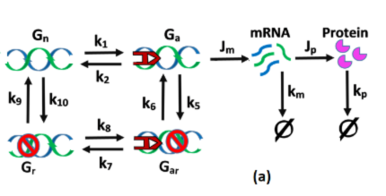
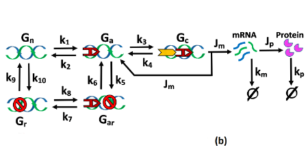
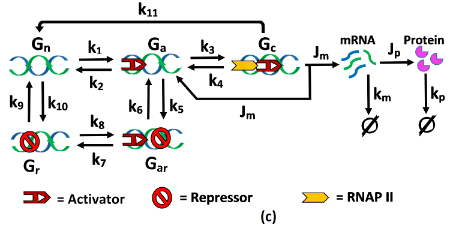
Figure 1: Reaction schemes for an activator-repressor system with non-competitive interaction of a gene. (a) Network without transcription reinitiation path: an activator binds to the promoter of gene at normal state ($G_{n})$ to make the gene active ($G_{a})$ for synthesis of mRNA. Proteins are then produced from mRNA via reaction rate $J_{p}.$ $k_{m}$ and $k_{p}$ are the rates of decay of mRNA and proteins respectively. A repressor can bind to the normal state to make a repressed state $(G_{r})$ which is unable to transcribe. A repressor may also attach with an active state to bring the gene at an active-repressed state ($G_{ar}).$
(b) Network with a transcription reinitiation path from an initiation complex $G_{c}$ to $G_{a}$ via $J_{m}$. The state $G_{c}$ is formed when RNAP II binds to an active state ($G_{a}).$
(c) With transcription reinitiation path and a direct transition path from the closed complex $G_{c}$ to the normal state $G_{n}$.

It should be stressed that, the reaction scheme of the gene regulatory network in figure 1(c) is the more general one compared to figure 1(b). So, we write the Master equation [32] corresponding to the reaction scheme in figure 1(c) and calculate the mean and the Fano factor of mRNAs and proteins at the steady state.

We assume that there exists $l$ copy number of a particular gene in the cell. Let us consider $p(n_{1},n_{2},n_{3},n_{4},n_{5},n_{6},t)$ be the probability that at time $t$, there are $n_{5}$ number of mRNAs and $n_{6}$ number of protein molecules with $n_{1}$ number of genes in the active state ($G_{a}$), $n_{2}$ number of genes in the initiation complex ($G_{c}$), $n_{3}$ number of genes in the active-repressed state ($G_{ar}$) and $n_{4}$ number of genes in the repressed ($G_{r}$) state. The number of gene in the normal states ($G_{n}$) are $(l-n_{1}-n_{2}-n_{3}-n_{4})$. The time evaluation of the probability is given by

$$\begin{array}[]{ccc}\frac{\partial p(n_{i},t)}{\partial t}&=&k_{1}[\{l-(n_{1}-1+n_{2}+n_{3}+n_{4})\}p(n_{1}-1,n_{2},n_{3},n_{4},n_{5},n_{6},t)\\ &&-\{l-(n_{1}+n_{2}+n_{3}+n_{4})\}p(n_{i},t)]\\ &&+k_{2}[(n_{1}+1)p(n_{1}+1,n_{2},n_{3},n_{4},n_{5},n_{6},t)-n_{1}p(n_{i},t)]\\ &&+k_{3}[(n_{1}+1)p(n_{1}+1,n_{2}-1,n_{3},n_{4},n_{5},n_{6},t)-n_{1}p(n_{i},t)]\\ &&+k_{4}[(n_{2}+1)p(n_{1}-1,n_{2}+1,n_{3},n_{4},n_{5},n_{6},t)-n_{2}p(n_{i},t)]\\ &&+k_{5}[(n_{1}+1)p(n_{1}+1,n_{2},n_{3}-1,n_{4},n_{5},n_{6},t)-n_{1}p(n_{i},t)]\\ &&+k_{6}[(n_{3}+1)p(n_{1}-1,n_{2},n_{3}+1,n_{4},n_{5},n_{6},t)-n_{3}p(n_{i},t)]\\ &&+k_{7}[(n_{3}+1)p(n_{1},n_{2},n_{3}+1,n_{4}-1,n_{5},n_{6},t)-n_{3}p(n_{i},t)]\\ &&+k_{8}[(n_{4}+1)p(n_{1},n_{2},n_{3}-1,n_{4}+1,n_{5},n_{6},t)-n_{4}p(n_{i},t)]\\ &&+k_{9}[(n_{4}+1)p(n_{1},n_{2},n_{3},n_{4}+1,n_{5},n_{6},t)-n_{4}p(n_{i},t)]\\ &&+k_{10}[\{l-(n_{1}+n_{2}+n_{3}+n_{4}-1)\}p(n_{1},n_{2},n_{3},n_{4}-1,n_{5},n_{6},t)\\ &&-\{l-(n_{1}+n_{2}+n_{3}+n_{4})\}p(n_{i},t)]\\ &&+k_{11}[(n_{2}+1)p(n_{1},n_{2}+1,n_{3},n_{4},n_{5},n_{6},t)-n_{2}p(n_{i},t)]\\ &&+J_{m}[(n_{2}+1)p(n_{1}-1,n_{2}+1,n_{3},n_{4},n_{5}-1,n_{6},t)-n_{2}p(n_{i},t)]\\ &&+k_{m}[(n_{5}+1)p(n_{1},n_{2},n_{3},n_{4},n_{5}+1,n_{6},t)-n_{5}p(n_{i},t)]\\ &&+J_{p}[n_{5}p(n_{1},n_{2},n_{3},n_{4},n_{5},n_{6}-1,t)-n_{5}p(n_{i},t)]\\ &&+k_{p}[(n_{6}+1)p(n_{1},n_{2},n_{3},n_{4},n_{5},n_{6}+1,t)-n_{6}p(n_{i},t)]\end{array}$$ (1)

where, i = 1,2,……, 6

We can derive the mean, variance and the Fano factor of mRNAs and proteins from the moments of equation (1) with the help of a generating function. The mean mRNA and protein are given by

$$m^{WR}=\frac{J_{m}k_{3}k_{8}b_{9}b_{2}}{k_{m}(-k_{3}k_{8}(b_{11}b_{1}+b_{10}k_{10})-(b_{11}b_{13}-b_{10}b_{12})b_{2})};\quad p^{NCWR}=\frac{m^{WR}\,J_{p}}{k_{p}}$$ (2)

$$FF_{m}^{WR}=1+A-m^{WR}$$ (3)

$$FF_{p}^{WR}=1+B-p^{WR}$$ (4)

where the detail expressions of A, B and C along with other $b_{j}$(j=1,2,……,20) parameters are given in Appendix-B.

In the following analyses we have emphasized only on a subset of the set of parameters that appear in equation (1). In this way, we have successfully established how the same set of parameters considered in [3] also affects the physical quantities that we can calculate for the configuration 1(c). An additional advantage in working with the same set of parameters is that, in the limiting case we can reproduce the results of [3, 26, 28].

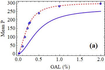
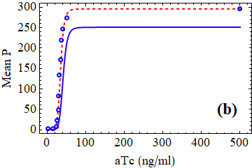
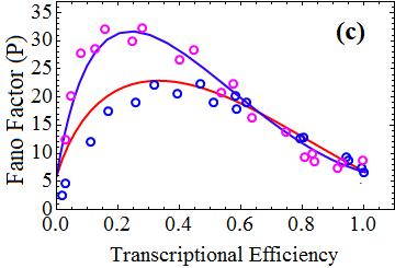
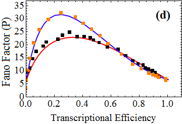
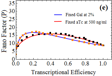
Figure 2: Variation of mean protein with (a) GAL at full aTc and (b) aTc at 2% GAL. Solid (dashed) line is drawn from analytical calculation corresponding to scheme 1(a) (figure 1(b)). Hollow circles are the experimental data points with 2% GAL concentration in (b) and with aTc=500 ng/ml in (a).
(c) and (d) represent the variation of the Fano factor with transcriptional efficiency. In (c), blue (red) solid line is drawn analytically with 2% GAL concentration (with aTc=500 ng/ml) from the scheme 1(b). In (d), blue (red) solid line is drawn analytically with 2% GAL concentration (with aTc=500 ng/ml) from configuration 1(b). The black and brown squares are generated from stochastic simulation using the Gillespie algorithm [33] from the reactions in figure 1(c). In (e), the red (blue) solid line is from exact analytical expression and squares are from stochastic simulation according to the configuration 1(a).

In Figure 2, we have shown the variation of mean and the Fano factor of proteins with respect to external inducers and transcriptional efficiency. In the next step, we verify our analytical results by matching the expressions of mean and the Fano factor calculated from the reaction schemes in figure 1 with the experimental data points in [3]. Note that, in this analysis we have considered the rate constants and the reaction scheme of [3] which corresponds to the figure 1(b). We also draw the curves for the mean (2(a,b)) and the Fano factor (2e) without the reinitiation process, correspondig to configuration 1(a). Subsequently, we compare the effect of reinitiation of transcription on those two quantities. We find similar conclusion as in [3] that reinitiation can increase both the noise and mean expression level. Both the experimental data and our analytical results show that the reinitiation of transcription process in the present transcriptional regulatory architecture increases the Fano factor at the protein level (figure 2(d) and (e)). We also see that the reinitiation of transcription increases the mean protein level compared to the transcription without reinitiation [28]. The rate constants used in [3] are given by $k_{1}=0.02+0.2*GAL,$ $k_{2}=0.01+0.1*GAL+0.077/GAL$, $k_{3}=50,k_{4}=10,k_{5}=e*k_{10},\,k_{10}=200*(npt)^{2}/[1+(C_{i}*aTc)^{4}]^{2},\>k_{6}=k_{9}=10,$$\,k_{8}=e*k_{1},k_{7}=k_{2},J_{m}=1,k_{m}=1,J_{p}=5,k_{p}=0.0125,npt=100,C_{i}=0.1,e=0.025$. A better fitting with a different set of rate constants (using reaction scheme 1c) is shown in the following paragraph by considering extra intermediate possible transitions. We have analytically find the idea of another set of rate constants that can give a better fitting of data.

In figure 2(c), we see that the analytical curve for variation of the Fano factor with transcriptional efficiency for fixed aTc at 500 ng ml^-1 differ greatly with experimental data points at lower values of transcriptional efficiency. Now we tried for a different set of rate constants to remove this discrepancy. We use the reaction scheme shown in figure 1(c) where a direct path of possible transition from $G_{c}$ to $G_{n}$ via $k_{11}$ has been considered, as both the activator and RNAP II can remove simultaneously from the stage $G_{c}$ to bring back the gene at stage $G_{n}.$ Also, the intermediate genetic stages between G_n and $G_{c}$ are considered which were ignored earlier.

We assume when the activator molecules are attached to $G_{n}$, there exists an intermediate state $G_{s}$ (Gene-dox complex). The activation rate constant $k_{A}$ carries dox [s] whereas deactivation rate $k_{D}$ releases dox from $G_{s}.$ We choose $k_{A}=k_{a}[s]$ and $k_{D}=k/k_{A}=k_{d}/[s]$, where $k$ is a constant of proportionality. There are a direct basal path $k_{B}$ (forward) and $k_{R}$ (reverse) from $G_{n}$ to $G_{a}.$

Let us consider :

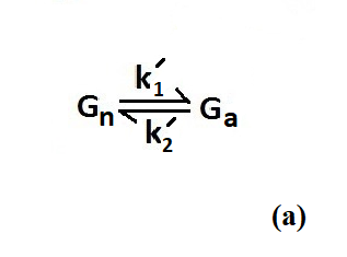
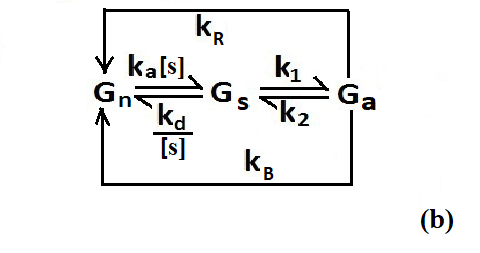
Figure 3: Intermediate state consideration: (a) our consideration with equivalent reaction rates between normal state $(G_{n})$ and active state ($G_{a})$. (b) generalized structure with intermediate state $G_{s}$ (Gene-dox complex).

The kinetic equations are :

$$\frac{d[G_{a}]}{dt}=k_{1}[G_{s}]+k_{B}[G_{n}]-(k_{2}+k_{R})[G_{a}]$$ (5)

$$\frac{d[G_{s}]}{dt}=k_{a}[s][G_{n}]-\frac{k_{d}}{[s]}[G_{s}]+k_{2}[G_{a}]-k_{1}[G_{s}]$$ (6)

$$\frac{d[G_{n}]}{dt}=\frac{k_{d}}{[s]}[G_{s}]+k_{R}[G_{a}]-(k_{a}[s]+k_{B})[G_{n}]$$ (7)

$$[G_{n}]+[G_{s}]+[G_{a}]=1$$ (8)

Applying steady state condition, $\frac{d[G_{a}]}{dt}=0,\frac{d[G_{s}]}{dt}=0,\frac{d[G_{n}]}{dt}=0$ and solving we get

$$[G_{a}]=\frac{k_{1}^{{}^{\prime}}}{k_{1}^{{}^{\prime}}+k_{2}^{{}^{\prime}}}$$ (9)

where,

$$k_{1}^{{}^{\prime}}=k_{1}[k_{a}[s]+\frac{k_{B}}{k_{1}}\frac{k_{d}}{[s]}+k_{B}]$$ (10)

$$k_{2}^{{}^{\prime}}=k_{2}^{c}[k_{a}[s]+\frac{k_{d}}{[s]}+k_{c}$$ (11)

with $k_{2}^{c}=(k_{2}+k_{R})$ and $k_{c}=\frac{k_{1}k_{R}+k_{2}k_{B}}{k_{2}^{c}}$.

When the intermediate state $G_{s}$ is absent, we have the same form of $G_{a}$ as shown in equation (9). Now from equations (10) and (11) we can see the exact form for the GAL dependent rate constants $k_{1}$ and $k_{2}$. Using trial and error method with different numerical values we are able to fit the experimental data with theoretical curves. The availability of the analytical expression of the Fano factor as a function of different rate constants helps us to do that very easily. The new set of rate constants are given by $k_{1}=0.0002/GAL+0.027+0.13*GAL,$ $k_{2}=0.002+0.1*GAL+0.06/GAL$, $k_{3}=50.0,k_{4}=12.5,k_{5}=e*k_{10},k_{10}=200*(npt)^{2}/[1+(C_{i}*aTc)^{4}]^{2},\>k_{4}=k_{9}=10,$$k_{11}=0.005$,$k_{7}=e*k_{1},k_{8}=k_{2},J_{m}=2.5,k_{m}=1,J_{p}=2.3,k_{p}=0.0125,npt=100,C_{i}=0.1,e=0.025$. From figure (4) we observe that the analytical curves for the variation of mean and the Fano factor well agree with the experimental data points. With the new set of rate constants mentioned above, the nature of variation of mean and the Fano factor at protein level do not change. The best estimated values of parameters and their uncertainties are discussed in Appendix-E.

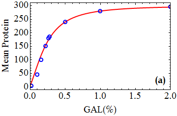
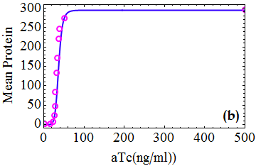
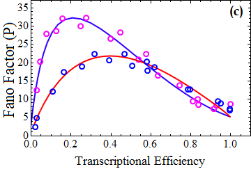
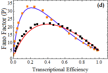
Figure 4: Variation of mean protein with (a) GAL at aTc=500 ng/ml and (b) aTc at 2% GAL. Solid lines are drawn from analytical calculation corresponding to the figure 1(c). Hollow circles are the experimental data points with 2% GAL concentration in (b) and aTc=500 ng/ml in (a).
(c) and (d) shows the variation of the Fano factor with transcription efficiency. Blue (red) solid line is drawn analytically with 2% GAL concentration (with aTc=500 ng/ml) from the configuration 1(c). In (d), the black and orange squares are are generated from stochastic simulation using the Gillespie algorithm from the reactions in configuration 1(c) and the rate constants are given in the text above.

The plots figure (5) show the variation of mean protein with GAL (figure 5(a)) at different aTc and with aTc (figure 5(b)) at different GAL concentrations. It can be visualized that, for GAL $\geq$2% mean protein attains saturation at aTc $\approx$ 60 $ng$ $ml^{-1},$ whereas for GAL < 2% mean protein increases rapidly for aTc > 20 $ng$ $ml^{-1}.$ Figure 5(b) also showing that the mean protein is almost independent of GAL when reinitiation is taken into consideration.

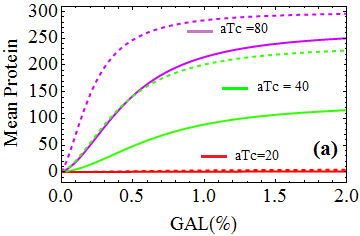
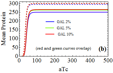
Figure 5: Variation of mean (a) with GAL at different aTc concentration and (b) with aTc at different GAL (%) concentration. The solid curves correspond to the configuration 1(a) and the dashed curves are corresponding to the configuration 1(b).

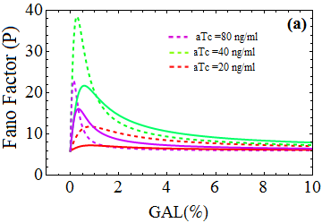
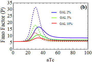
Figure 6: Variation of the Fano factor with (a) GAL (%) at different aTc and (b) aTc at different GAL (%) concentration.The dashed curves are drawn from analytical calculations corresponding to the scheme 1(b).

In figure 6(a), we plot the Fano factor with GAL at different aTc. In figure 6(b), the variations of the Fano factor with aTc for different GAL concentrations are shown. It is clear from figure 6(a) that the Fano factor is maximum at aTc = 40 ng ml^-1 as compared to aTc = 20 and 80 ng ml^-1. The Fano factor is higher at lower GAL concentration when observed with aTc variation. We present the corresponding 3D plots in figure (7) to have a clearer view of the variation of mean and the Fano factor of protein and mRNA with respect to GAL and aTc concentration. We observe from figure (7) that both the mean and the Fano factor vary with GAL and aTc. Howerver it is interesting to note that, when we increase GAL concentration from 2% to 10%, the Fano factor decreases accordingly (figure 6b). On the other hand, figure 5(b) shows that the changes in the mean protein level is extremely small without reinitiation, whereas negligible changes are observed when reinitiation of transcription is included and mean protein level becomes nearly independent of GAL. Similar conclusion was drawn in [13] as well. However, here we have pointed out that this conclusion is valid effectively only when reinitiation is involved (figure 5b and 6b).

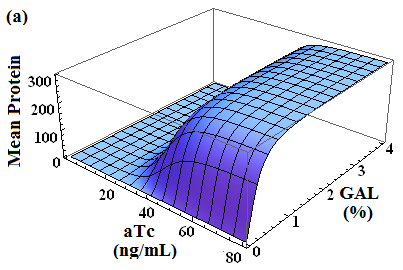
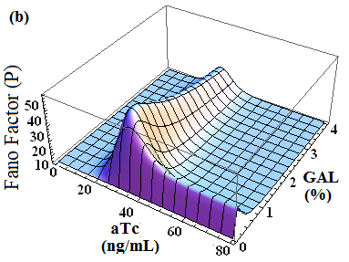
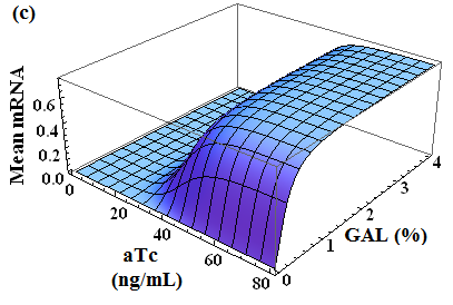
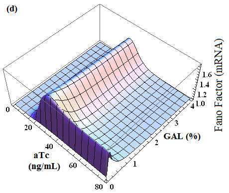
Figure 7: Variation of mean and the Fano factor at protein and mRNA levels obtained from analytical calculations with aTc and GAL corresponding to the scheme 1(b). The rate constants are chosen from Blake et al. [3]. (a) and (b) are reproduced as in [13].

In figure 7(a) and (b), we reproduce the variation of mean protein and the Fano factor against aTc and GAL (as in [13]) by means of our analytical calculation. Then we examine that the similar behavior of mean and the Fano factor against GAL and aTc are followed by mRNA, as expected. We can see there is a resonance type of incident for aTc $\approx$ 30 $ng$ $ml^{-1}$ and GAL $\approx$ 0.5% (for the set of rate constant given in [3] which gives a sudden peak in the Fano factor (noise strength)). The critical value of aTc, as a function of GAL, for maximum Fano factor can be computed analytically. The final expression is too large and hard to simplify, and hence we avoid writing it here. Although, for a particular set of numerical values of rate constants, we can determine the critical aTc value from our analytical expression.

2.1 The Fano factor in the sub-Poissonian region

The reinitiation process at the transcriptional level is crucial for the reproduction of experimental results from stochastic simulation of the model network in [3]. Our analytical study of the same model network shows that the reinitiation process increases the Fano factor at the protein levels (figure 2e). The effect of reinitiation is observed first at the mRNA levels. Figure 7(d) shows that the Fano factor at the mRNA level also increases due to the reinitiation process for the given rate constants. Our analysis also reveals that the reinitiation process at the transcription level can bring down the Fano factor at the mRNA level to the sub-Poissonian regime [26, 28]. At this stage, we would like to check whether it is possible to observe the sub-Poissonian Fano factor due to reinitiation dynamics in this non-competitive regulatory architecture (configuration 1b).

In order to achieve that, we find the critical condition for $J_{m}$ by imposing the inequality $FF_{m}<1$ on equation (3). The resulting expression of critical $J_{m}$, i.e., $J_{m}^{c}$ is given by

$$J_{m}^{c}<\frac{B_{1}-B_{2}-B_{3}}{B_{4}-B_{5}+B_{6}}$$ (12)

where,

$B_{1}=b_{8}[b_{9}\{\left(b_{12}+k_{5}k_{m}\right)\left(k_{m}+k_{r}\right)-k_{3}k_{8}k_{10}\}$

$-k_{10}\left(b_{11}\left(b_{13}k_{r}+k_{3}\left(k_{4}-k_{1}\right)k_{8}\right)-b_{10}\left(b_{12}k_{r}-k_{3}k_{8}k_{10}\right)\right)]$

$B_{2}=\left(b_{16}\left(k_{m}+k_{1}\right)+b_{4}k_{1}k_{10}\right)\{b_{10}\left(b_{12}k_{r}-k_{3}k_{8}k_{10}\right)$

$\hskip 20.075pt-b_{11}\left(b_{13}k_{r}+k_{3}\left(k_{4}-k_{1}\right)k_{8}\right)\}$

$B_{3}=b_{9}[b_{13}b_{16}\left(k_{m}+k_{r}\right)-b_{16}k_{8}\left(k_{m}\left(k_{m}+k_{r}\right)+k_{1}k_{3}-k_{4}k_{3}\right)$

$\hskip 20.075pt+b_{4}k_{1}\left(b_{12}\left(k_{m}+k_{r}\right)+k_{5}k_{m}\left(k_{m}+k_{r}\right)-k_{3}k_{8}k_{10}\right)]$

$B_{4}=\left(b_{10}b_{12}-b_{11}\left(b_{13}+k_{3}k_{8}\right)\right)\left(b_{16}\left(k_{m}+k_{1}\right)+b_{4}k_{1}k_{10}\right)$

$B_{5}=b_{8}\left(b_{9}\left(b_{12}+k_{5}k_{m}\right)+k_{10}\left(b_{10}b_{12}-b_{11}\left(b_{13}+k_{3}k_{8}\right)\right)\right)$

$B_{6}=b_{9}\left(b_{16}k_{8}\left(k_{3}-k_{m}\right)+b_{4}k_{1}\left(b_{12}+k_{5}k_{m}\right)+b_{13}b_{16}\right)$

and $k_{r}=k_{4}+k_{11}$.

The details of $b_{j}$ parameters are given in Appendix-B.

We will see that these factors within $k_{r}$ have a big role in controlling noise for the circuit.

The presence of the critical value (which gives Poissonian Fano factor at mRNA levels) $J_{m}^{c}$ in equation (12) shows that noncompetitive regulatory architecture with transcriptional reinitiation can give rise to three different regimes of the Fano factor, viz., sub-Poissonian, Poissonian and super-Poissonian as shown in [26, 28]. In figure (8) we plot the three different regions of the Fano factor along with the critical value of $J_{m}$ ($J_{m}^{c}$= 6.05) for the rate constants provided by Blake et al. [3]. The plots show that the reduction of Fano factor towards the sub-Poissonian regime is extremely small. However, the decrease in the value of the Fano factor towards the sub-Poissonian regime is greater with lower values of the rate constant $k_{4}$ (figure 8(b)). We also find the critical values of aTc and GAL corresponding to the rate constants in [3]. Additionally, these three different regimes of the Fano factor can also be observed for range of values of aTc and GAL as shown in figure (9).

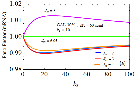
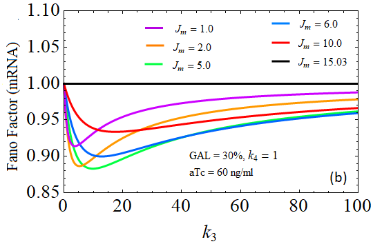
Figure 8: Plot of Fano factor at mRNA level with $k_{3}$ for different values of $J_{m}$ with 30% GAL concentrations and aTc = 60 ng ml^-1. (a) The other rate constants are chosen from Blake et al. [3]. (b) Here $k_{4}=1$. Other parameters are the same as in [3]. Lower value of $k_{4}$ helps to reduce the Fano factor more below the Poissonian level.

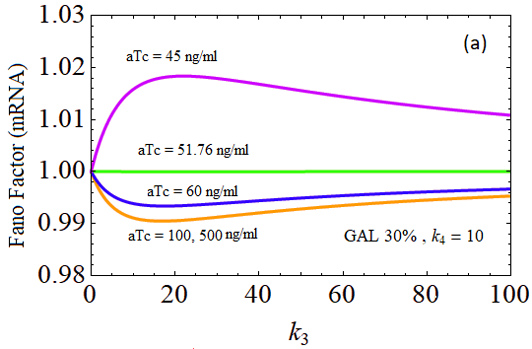
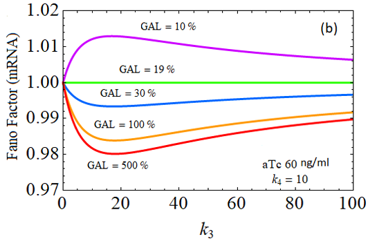
Figure 9: Plot of the Fano factor at mRNA level with $k_{3}$ with (a) aTc and (b) GAL as parameter. The other rate constants are chosen from Blake et al. [3].

In order to observe the variation of the Fano factor more clearly, we plot (3D) the Fano factor with $k_{3}$ and $J_{m}$ for different concentrations of aTc and GAL. Figure 10 show that the Fano factor can go below unity when aTc is more than 40 ng/ml with $30\%$ GAL concentrations. Consequently, we observe a valley/dip in the Fano factor (at protein levels) at aTc more than 40 ng/ml and $30\%$ GAL concentration, in figure (11). This observation is in sharp contrast to figure (7) where we observe peaks in the Fano factor rather than dips. We have also examined that the Fano factor at sub-Poissonian region as shown in figure (9) can not be reduced below the level presented by a two-state network with reinitiation [26, 28]. Whatever may be the values of other rate constants at aTc$\geq$100, our non-competitive model effectively reduces to a two-state model and can reproduce all the features as shown in [28]. This can be analytically shown (refer to section 2.2) that our proposed non-competitive architecture can be reduced to a two-state network at aTc→$\infty$ and $k_{11}=0.$

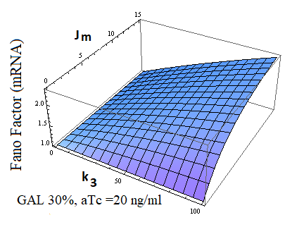
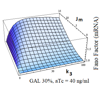
Figure 10: Variation of the Fano factor at mRNA level with $k_{3}$ and $J_{m}$ for different aTc concentrations with 30% GAL and $k_{4}=1$.

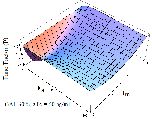
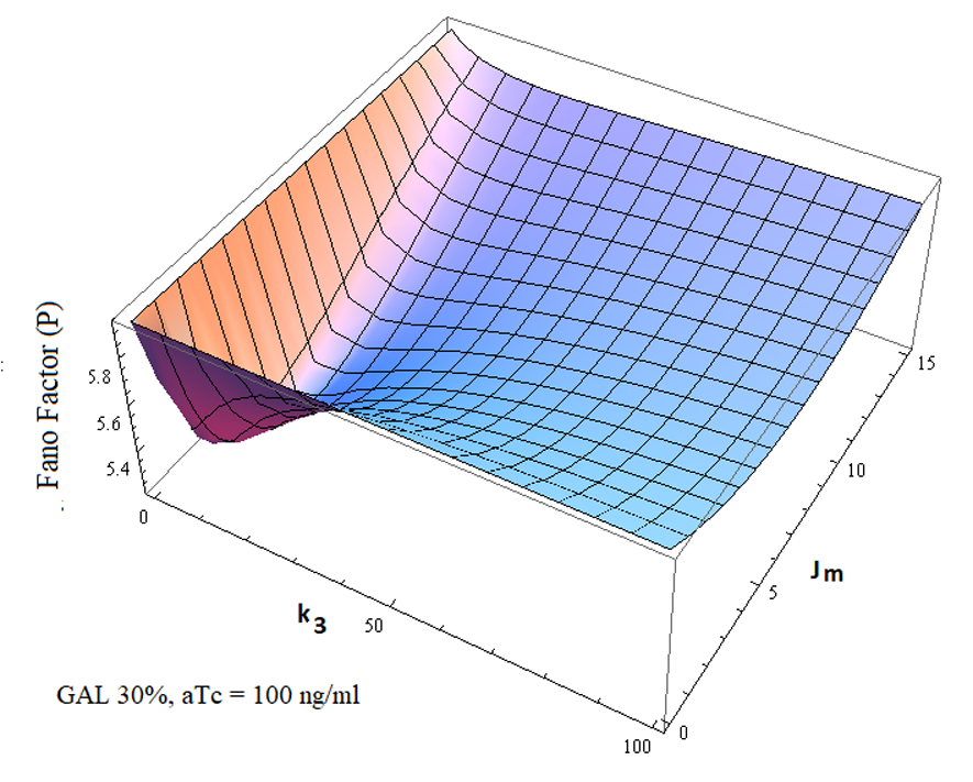
Figure 11: Variation of the Fano factor at protein level with $k_{3}$ and $J_{m}$ for different aTc concentrations and fixed GAL concentration (30%) and $k_{4}=1$. Here we find a dip rather than the peak (as in Figure 7) in the Fano factor at proten level due to reinitiation.

2.2 Role of aTc

Tetracycline (Tc) controlled gene expression has been exhibited in a variety of eukaryotic systems including Saccaromyces cerevisiae [57]. Although Tc has some good medicinal properties, its very little but distinct cytotoxicity to mammalian cells reduces its applicability. Rather, one of its derivatives, anhydrotetracycline (aTc), which binds the Tet repressor (TetR) more effectively than Tc, is widely used in activator-repressor systems. It has also a lower antibiotic activity towards E. coli [52]. A tetR (repressor) attached with aTc inhibits expression and produces noise in the expression. This repression is modeled by the aTc dependent transition rate $k_{10}\propto\frac{(tetR)^{2}}{[1+(C_{i}*aTc)^{4}]^{2}}$ and $k_{5}=ek_{10}$.

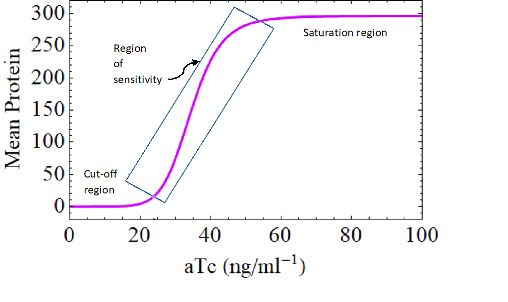
Figure 12: Mean protein vs. aTc

aTc (ng ml${}^{-1})$	20	25	30	35	40	50	65	80	100
$k_{10}$	6920	1250	297.53	87.64	30.28	5.01	0.78	0.119	0.019

Table 1: Sensitivity of $k_{10}$ to aTc concentration

The response of the non-competitive circuit is very sensitive to aTc concentration. Figure (12) exhibits a response (mean protein) versus aTc curve for non-competitive architecture.The curve has sigmoid nature and looks very similar to a output characteristic of a junction transistor having three region of operation viz. cut-off region, active region and saturation region. The active region is the region of interest known as “region of sensitivity”. In cut-off region of operation ($0\leq aTc\leq 25$) both the mean and noise is negligible. In the active region ($(25\leq aTc\leq 55$) mean expression increases sharply offering a larger noise (figure 5b and figure 6b). When the mean value reaches to saturation (aTc>55) the noise reduces to a very low level. For lower concentration of aTc the gene state is highly repressed that resists to express. Figures (5) to (11) explains how aTc plays an governing role in regulation of mean and noise. Table 1 shows the sensitivity of $k_{10}$ to aTc concentration. A small change in aTc results in a larger change in $k_{10}$. If we make aTc concentration significantly high which effectively blocks the transitions : towards $G_{r}$ from $G_{n}$ and towards $G_{ar}$ from $G_{a}$. For aTc→$\infty$ , both $k_{10}$ and $k_{5}$ (as $k_{5}=ek_{10})$ are effectively zero. Then, along with $k_{11}=0$ the reaction scheme 1(c) reduces to a two-state model with reinitiation path involved.

Under these two limits we have from equation (2),

$$m^{WR}=\frac{J_{m}k_{1}k_{3}}{k_{m}((J_{m}+k_{4})(k_{1}+k_{2})+(k_{1}k_{3}))}=\frac{J_{m}k_{1}k_{3}}{a_{2}^{{}^{\prime}}k_{m}}$$ (13)

and from equation (3),

$$FF_{m}^{WR}=1+\frac{J_{m}k_{3}(k_{1}+k_{m})}{(a_{1}^{{}^{\prime}}+a_{2}^{{}^{\prime}})k_{m}}-\frac{J_{m}k_{1}k_{3}}{a_{2}^{{}^{\prime}}k_{m}}$$

$$=1+\frac{J_{m}k_{3}(a_{2}^{{}^{\prime}}-a_{1}^{{}^{\prime}}k_{1})}{(a_{1}^{{}^{\prime}}k_{m}+a_{2}^{{}^{\prime}})a_{2}^{{}^{\prime}}}$$ (14)

Note that, equation (13) and equation (14) have the same form of the mean mRNA and the Fano factor (mRNA) of a two-state network with reinitiation given in [26, 28] with $a_{1}^{{}^{\prime}}=k_{1}+k_{2}+k_{3}+k_{4}+J_{m}+k_{m}$ and $a_{2}^{{}^{\prime}}=(J_{m}+k_{4})(k_{1}+k_{2})+k_{1}k_{3}$. Here we conclude that, practically, for aTc $\geq$100 and $k_{11}=0$ non-competitive network behaves like a two-state model producing all the plots as shown in [28].

2.3 Anomaly in the Fano factor (mRNA) at lower GAL concentration: role of $\boldsymbol{k_{11}}$

One of the major aspects of our work is the introduction of a direct transition path from the stage $G_{c}$ to $G_{a}$ [27], to the model previously studied by Blake et al. [3, 6]. We subsequently study the behavior of mean expressions and noise (in terms of the Fano factor) affected by the reaction rate $k_{11}$ for that path. As the gene expression is a complex process, we could not deny the possibility of simultaneous unbound of RNAP II and activator molecule and bring the gene to the normal state $G_{n}.$

With the rate constants used in [3] along with $k_{11}=0$, we notice from figure 13(a) that, when GAL < 5%, the maximum value of the Fano factor (at mRNA level ) without reinitiation is higher than that with reinitiation. The explanation of this behavior is subject to further analysis which we have not performed here. Nevertheless, we find that this anomaly goes off (i) for higher GAL concentrations and (ii) for the introduction of small non-zero value of $k_{11}$.

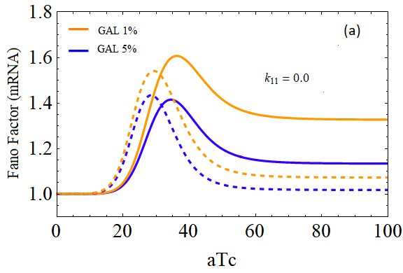
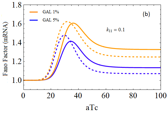
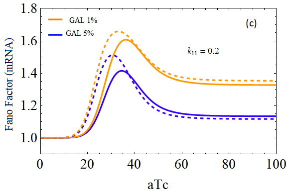
Figure 13: Variation of the Fano factor against aTc for GAL 1% and 5% with different $k_{11}$, solid lines correspond to configuration 1(a) and dashed lines correspond to configuration 1(c). Rate constants are chosen from [3].

We further observe from figure 13 that, the peak of the Fano factor curve (corresponding to the scheme 1c) has raised for $k_{11}=0.1$ and for $k_{11}=0.2$. This establishes the role of $k_{11}$ in raising the Fano factor up a bit. A non-zero, positive value of $k_{11}>0$ reduces the effective transition probabilities via rate constants $k_{2},k_{3},k_{4},k_{5},k_{6}$ and the transition from $G_{c}$ to mRNA via $J_{m}$ (see tables 3 and 4 in supplementary material). That helps to raise the Fano factor and hence removes that anomalous nature.

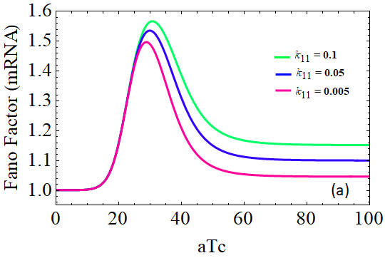
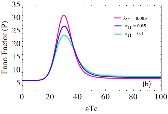
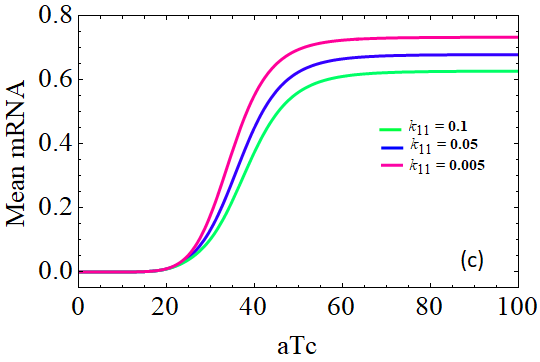
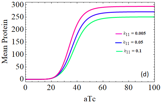
Figure 14: Role of $k_{11}$: (a) Fano factor (mRNA) vs. aTc, (b) Fano factor (protein) vs. aTc, (c) mean mRNA vs. aTc, (d) mean protein vs. aTc.
In these plots, different $k_{11}$ values are taken as parameter which reveal that, although mean values offering same behavior, the Fano factors are showing slightly different nature in transcription and translation level. Rate constants are chosen from [3].

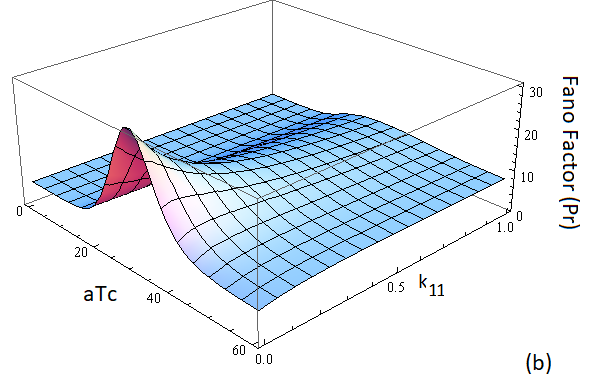
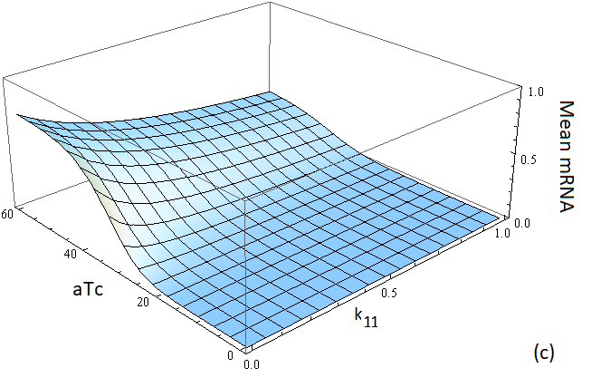
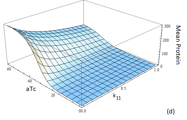
Figure 15: Role of $k_{11}$: 3D plot showing a clear difference in Fano factors at mRNA and protein level while variations of mean having similar nature. Rate constants are chosen from [3].

There are another very interesting role of $k_{11}$ as shown in figure (14) and figure (15). The plots of mean expressions (mRNA and protein) against aTc are decreasing with increasing $k_{11}$ values while the Fano factors at mRNA level (transcriptional) and that at protein level (translational) show some noticeable differences. The peaks of the Fano factors (mRNA level) are higher for higher values of the parameter $k_{11}$ but the peaks of the Fano factors at protein level decreases for higher values of $k_{11}.$ On the other hand, the horizontal linear portion of the Fano factor curve (right side of the curve 14b ) almost merges for different $k_{11}$values (aTc > 40) for proteins whereas the corresponding curves remain separated for mRNAs. This implies that the noise is different for different $k_{11}$ values at transcriptional level while it is almost same at translation level at higher aTc values (>40 ng ml${}^{-1})$.

2.4 Another noise reducing factor

We have found that the noise, corresponding to the circuit 1(c) can be reduced with the help of the factor e appearing in the rate constants in [3]. Without altering the maximum of mean expression (figure 16), we can reduce noise (denoted by the Fano factor here) by changing the value of the factor e. Figure 16(b) and (c) show that, an increasing e reduces the Fano factor much effectively in both transcription and translation levels. It can be observed (figure 16a) that the maximum and also the saturation value of mean protein remains unchanged with the increasing values of e except a little lateral shift in the “region of sensitivity”. This also reveals the fact that noise can be reduced when gene operates towards the active-repressed compound state ($G_{ar}).$ Generally, an additional genetic state (for linear circuits) causes much noise but here we see that extra states (squared architecture) reduce noise.

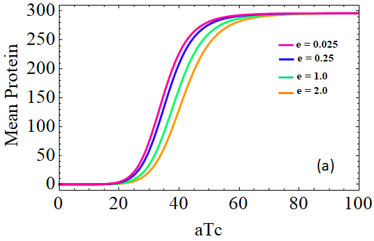
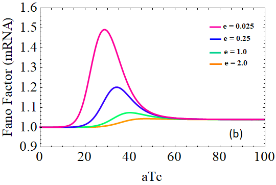
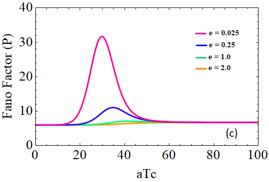
Figure 16: Role of the factor e : (a) variation of mean protein against aTc showing that saturation mean value does not change with different values of e except a little lateral shift in the region of sensitivity. (b) The Fano factor (mRNA) against aTc reduces with increasing value of e. (c) The Fano factor (protein) against aTc decreases with increasing e. Other rate constants are chosen from [3].

2.5 Anomalous peak in the variance of Protein against aTc

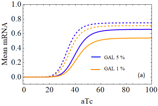
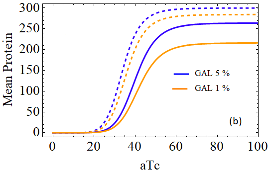
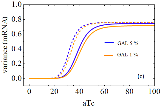
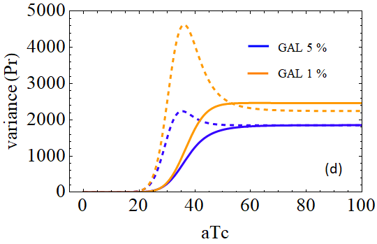
Figure 17: Variations of mean mRNA and mean Protein against aTc are plotted in (a) and (b) respectively. In (c) and (d) we plot of variance of mRNA and variance of protein against aTc repectively. Solid lines correspond to cofiguration 1(a) and dashed lines correspond to configuration 1(c). Rate constants are chosen from [3].

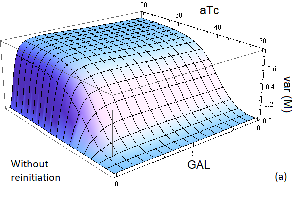
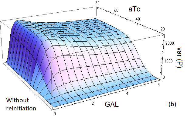
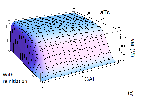
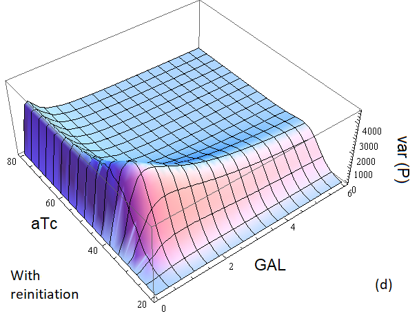
Figure 18: In (a) and (b) we plot variance of mRNA (var (M)) and variance of protein (var (P)) with GAL and aTc corresponding to configuration 1(a) and from the reaction scheme 1(c) we have the plots of variance at mRNA level (c) and that at protein level (d) against GAL and aTc. Rate constants are chosen from [3].

On top of that, using the same rate constants as in [3] along with $k_{11}=0$ we also found a sudden peak in the variance of protein against aTc (see figure 17d) in presence of trancriptional reinitiation corresponding to the process 1(b). This peak value increases with the reduction in GAL concentration. We find it interesting that the peak is not observed in variance of mRNA against aTc. Thus, one can predict that the peak is due to the process of translation. But a comparative 3D plot of variances of mRNA and protein (figure 18), with and without reinitiation (corresponding to the process 1(a) and 1(b), respectively), shows that the trancriptional reinitiation effect is responsible for it. We notice that the peak is near aTc $\approx$ 36.0 ng ml^-1. We prepare the following table that contains a number of transitions (for a single cell) between different genetic steps in gene expression for different aTc values.

(a) Without Reinitiation GAL 1%
aTc (ng ml-1)	$G_{n}$to $G_{a}$
via $k_{1}$	$G_{a}$to $G_{n}$
via $k_{2}$	$G_{a}$to $G_{c}$
via $k_{3}$	$G_{c}$to $G_{a}$
via $k_{4}$	$G_{a}$to $G_{ar}$
via $k_{5}$	$G_{ar}$to $G_{a}$
via $k_{6}$	$G_{ar}$to $G_{r}$
via $k_{7}$	$G_{r}$to $G_{ar}$
via $k_{8}$	$G_{r}$to $G_{n}$
via $k_{9}$	$G_{n}$to $G_{r}$
via $k_{10}$	$G_{c}$to $M$
via $J_{m}$	$M$ to $P$
via $J_{p}$
29.45	18	15	—–	—–	815	812	22	19	27319	27317	104	619
31.56	33	35	—	—	931	933	16	18	25885	25887	186	984
33.0	46	46	—	—	904	905	16	17	24612	24613	267	1410
34.73	60	63	—	—	684	684	12	15	23660	23664	330	1496
36.0	71	77	—	—	659	665	14	20	22269	22276	406	1876
40.0	126	126	—	—	470	470	12	12	17325	17325	676	3486

(b) With Reinitiation GAL 1% $k_{11}=0$
aTc (ng ml-1)	$G_{n}$to $G_{a}$
via $k_{1}$	$G_{a}$to $G_{n}$
via $k_{2}$	$G_{a}$to $G_{c}$
via $k_{3}$	$G_{c}$to $G_{a}$
via $k_{4}$	$G_{a}$to $G_{ar}$
via $k_{5}$	$G_{ar}$to $G_{a}$
via $k_{6}$	$G_{ar}$to $G_{r}$
via $k_{7}$	$G_{r}$to $G_{ar}$
via $k_{8}$	$G_{r}$to $G_{n}$
via $k_{9}$	$G_{n}$to $G_{r}$
via $k_{10}$	$G_{c}$to $M$
via $J_{m}$	$M$ to $P$
via $J_{p}$
29.45	19	18	3716	3348	620	619	17	16	24497	24497	368	1980
31.56	20	24	5622	5052	551	555	9	13	22049	22054	570	3141
33.0	30	33	7581	6857	503	506	8	11	19636	19639	724	3753
34.73	38	41	11962	10845	562	566	6	10	14558	14562	1116	5673
36.0	43	48	10921	9892	420	425	4	9	15355	15361	1029	5252
40.0	68	68	15364	14026	244	245	3	4	9570	9571	1338	6648

Table 2: Different genetic transitions for different aTc concentrations

We choose some random values of aTc and find out the different number of transitions for a single cell with the help of a simulation based on the Gillespie algorithm [33]. It can be seen from table 2(b) that, the transitions via $k_{3},k_{4},J_{m}$ and $J_{p}$ initially increase with aTc and drop suddenly at aTc = 36 ng ml^-1. Whereas, transitions via $k_{9}$ and $k_{10}$ initially decrease with aTc and undergoes a sudden rise in number of transitions at aTc = 36 ng ml^-1. It is to be noticed that although the variance of protein has a peak around aTc = 36 ng ml^-1, due to the value of mean protein, the maximum Fano factor (protein) is around aTc = 30 ng ml^-1 instead of aTc = 36.0 ng ml^-1. At this point, on the basis of figure 17(a) and (b), one can ask whether the mean values of mRNAs and proteins from reaction scheme 1(b) (i.e. with reinitiation ) can always be greater than those obtained from the process 1(a) (i.e. without reinitiation) for any other parameters. We found the answer to be in the negative. This has been explained in detail at Appendix-D.

3 Conclusions

Regulation of gene expression and control of noise have many biological and pharmacological significance [37, 38, 56]. Transcription factors (activators and repressors), that initiates the regulation of gene expression, can act as a tumor suppressor in prostate cancer [37]. Stochastic gene expression fluctuations (i.e. noise) are used to modulate reactivation of HIV from latency- a quiescent state that is a major barrier to an HIV cure. Noise enhancers reactivates latent cells, while noise suppressors stabilized latency [56].

In this paper, we have studied a gene transcription regulatory architecture observed in synthetic yeast GAL1^∗ promoter. Activator and repressor molecules bind the GAL1^∗ promoter in a non-competitive fashion to regulate the transcription. We focus on the reinitiation of transcription by RNAP II as suggested by Blake et al. [3, 6]. In our recent works [26, 28], we have found that the Fano factor (at mRNA level) goes well below the sub-Poissonian region and, after attaining a minima, it raises towards the super-Poissonian regime crossing the Poissonian level. Now, we have made an attempt to check whether the same nature of the Fano factor is valid in a four-state process when both activator and repressor are in action. We found the result in the positive. We have illustrated more effect of trancriptional reinitiation on the non-competitive network along with $k_{4}$ and aTc. We noticed that the Fano factor (protein) can have a dip rather than a peak as observed in [13].

Some aTc dependent features were observed by Blake et al. using reaction scheme 1(b) in [6] and they have claimed that the noise in gene expression is promoter-specific. We observed from figure (7) that both the mean and the Fano factor vary with GAL and aTc; whereas, only the Fano factor can be varied with aTc considering GAL as a parameter. Figures 5(b) and 6(b) show that the Fano factor can be varied with GAL though the mean protein level (with reinitiation) is almost independent of GAL. Similar conclusion was drawn in [13] as well. But we have pointed out that this conclusion is valid only when the reinitiation is involved (figure 5b and 6b).

In [6] the authors have shown the time dependence behavior of noise with aTc concentration as a function of time in their network. Whereas we have focussed on the dependence of noise on different reaction rates. As we have included the extra path (fig. 1c and 3b) of possible interactions and reduced the approximations to possible extent, our network and calculations became more complex and more general. In our analytical computation, we have found expressions for mean and the Fano factor at mRNA and protein levels. This can indeed be useful for further rigorous study of non-competitive network via any of its parameters. The analytical expression of the Fano factor with transcriptional efficiency has been matched with the experimental data points of [3]. Our analytical curves and the simulation results are similar to those of [3]. Moreover, the experimental data points and the analytical curve for the Fano factor (figure 2c) at full aTc have a mismatch for lower transcriptional efficiency. So we tried for the different set of rate constants to match the analytical results and experimental data points of [3]. Along with the consideration of extra paths, the availability of analytical expressions enables us to do that efficiently. We have found analytically a different set of rate constants that matches the experimental data points of mean and the Fano factor for all values of transcriptional efficiency. We also observe that the choice of rate constants is not unique. There can be other sets of rate constants that may give good fitting of analytical curves with the experimental data points. The minimization of relative error and mean squared error support the robustness of our model estimations of parameters (see Appendix-E).

We checked how mean, Fano factor and variance behave in presence of both activator and repressor. Among these two, repressor (bound by aTc) has more governing role to the regulation of noise. There are three regions of operation of aTc. Along with this, the reaction rates $k_{4}$ and $k_{11}$ are also important nobs in noise regulation. Also the factor e appearing in the reaction rates, can play a significant role in reducing noise in presence of highly active aTc concentration.

We noticed that there are some anomalous nature of the Fano factor of mRNA and variance of protein against aTc at lower GAL concentration (<5%). It is very interesting that although non-competitive network has more noise than that of a two-state process, noise can be reduced to sub-Poissonian region. But it can not be reduced below the level presented by a two-state network with the help of transcriptional reinitiation [47]. We observed that although mean mRNA against GAL or against aTc for a network with trancriptional reinitiation is higher than that of a network without reinitiation but mean mRNA can be both higher or lower when we plot them against other rate constants (considering as variable).

For $k_{11}=0$ the reaction scheme 1(c) is same as 1(b) that was proposed by Blake et al. [3]. From analytical expressions it has been shown that in the limit of aTc→$\infty$ and $k_{11}=0$ our model (reaction scheme 1(c)) reduces to a well established two-state model with reinitiation producing all the equations and plots as in [26, 28]. We have found this can be achieved at aTc = 100 practically.

Along with this model, we conducted a parallel study of an activator-repressor binding competitive network. We found a higher noise there in comparison with the non-competitive binding. However the mean remains same for the identical set of rate constants [54]. A similar experimental work was developed by Rossi et al. [55] and argued that activator and repressor binding may work as a rheostat in putting on/off a gene. Braichencho et al. [50] modeled a three-state activator-repressor system where there is a proximal promoter-pausing which can be effectively described by a two-state model. Another competitive model has been proposed recently in [53] where the regulation of gene expression by TFs can occur via two cross talking parallel pathways : basal and external signal.

Our proposed model may put an interest in synthetic biology, where an engineering design approach is being studied to understand the modified functionality of a biological system. From the analytical approach, it is possible to predict the average and standard deviation of the number of transcribed proteins. This model is useful to understand the architecture of interactions which may buffer the stochasticity inherent to gene transcription. There can be further extensive study on the model considering the effect of other parameters that are not included in present analysis.

                                    Appendix - A

In an attempt to deduce the expressions of mean and the Fano factors, we use a moment generating function which is defined as,

$$F(z_{i},t)=\sum_{n=0}^{\infty}z_{i}^{n_{i}}p(n_{i},t)$$ (15)

Here, $i=1,2,......,6$.

we have,

$$\begin{array}[]{ccc}\frac{\partial F(z_{i},t)}{\partial t}&=&\sum_{n=0}^{\infty}z_{i}^{n_{i}}\frac{\partial p(n_{i},t)}{\partial t}\\ &=&k_{1}(z_{1}-1)[lF-z_{1}\frac{\partial F}{\partial z_{1}}-z_{2}\frac{\partial F}{\partial z_{2}}-z_{3}\frac{\partial F}{\partial z_{3}}-z_{4}\frac{\partial F}{\partial z_{4}}]\\ &&+k_{2}(1-z_{1})\frac{\partial F}{\partial z_{1}}+k_{3}(z_{2}-z_{1})\frac{\partial F}{\partial z_{1}}+k_{4}(z_{1}-z_{2})\frac{\partial F}{\partial z_{2}}\\ &&+k_{5}(z_{3}-z_{1})\frac{\partial F}{\partial z_{1}}+k_{6}(z_{1}-z_{3})\frac{\partial F}{\partial z_{3}}+k_{7}(z_{4}-z_{3})\frac{\partial F}{\partial z_{3}}\\ &&+k_{8}(z_{3}-z_{4})\frac{\partial F}{\partial z_{4}}+k_{9}(1-z_{4})\frac{\partial F}{\partial z_{4}}\\ &&+k_{10}(z_{4}-1)[lF-z_{1}\frac{\partial F}{\partial z_{1}}-z_{2}\frac{\partial F}{\partial z_{2}}-z_{3}\frac{\partial F}{\partial z_{3}}-z_{4}\frac{\partial F}{\partial z_{4}}]\\ &&+k_{11}(1-z_{2})\frac{\partial F}{\partial z_{2}}+J_{m}(z_{1}z_{5}-z_{2})\frac{\partial F}{\partial z_{2}}+k_{m}(1-z_{5})\frac{\partial F}{\partial z_{5}}\\ &&+J_{p}(z_{6}-1)z_{5}\frac{\partial F}{\partial z_{5}}+k_{p}(1-z_{6})\frac{\partial F}{\partial z_{6}}\end{array}$$ (16)

In steady state, $\frac{\partial F(z_{i},t)}{\partial t}=0$ and for total probability, $F((z_{i}=1,0)=1$

Now, by setting [$\frac{\partial}{\partial z_{1}}(\frac{\partial F}{\partial t})]_{z_{i}=1}=0$, we get $\frac{\partial F}{\partial z_{1}}=f_{1}(say)=\thinspace<n_{1}>\thinspace=$ average number of gene at state $G_{a}$.

similarly, by setting [$\frac{\partial}{\partial z_{1}}(\frac{\partial^{2}F}{\partial z_{1}\partial t})]_{z_{i}=1}=0$ will give $\frac{\partial^{2}F}{\partial z_{1}^{2}}=f_{11}(say)$ and so on. Proceeding in the same way we obtain ,

$$f_{5}=\thinspace<n_{5}>\thinspace=mean\thinspace mRNA$$

and

$$f_{6}=\thinspace<n_{6}>\thinspace=mean\thinspace Protein$$

$$Fano\thinspace factor\thinspace(mRNA)=\frac{variance\thinspace of\thinspace mRNA}{mean\thinspace mRNA}=\frac{f_{55}+f_{5}-f_{5}^{2}}{f_{5}}$$

$$Fano\thinspace factor\thinspace(Protein)=\frac{variance\thinspace of\thinspace Protein}{mean\thinspace Protein}=\frac{f_{66}+f_{6}-f_{6}^{2}}{f_{6}}$$

                    Appendix - B

The parameters used in equation (2),(3) and (4) are given below

$A=-\frac{b_{19}J_{m}}{b_{20}k_{m}}$, $B=[\frac{J_{p}}{k_{m}+k_{p}}-\frac{J_{m}J_{p}k_{8}k_{3}^{2}(k_{10}(b_{8}-b_{5}k_{1})-b_{15}k_{1})}{b_{14}k_{p}(k_{m}+k_{p})}+\frac{b_{18}k_{8}(k_{m}+k_{1})}{(b_{8}-b_{4}k_{1})b_{14}(k_{m}+k_{p})}+\frac{b_{19}}{b_{20}}C]$,
$C=\frac{b_{17}}{b_{14}(k_{m}+k_{p})}-\frac{J_{m}J_{p}}{k_{m}(k_{m}+k_{p})}-\frac{b_{1}b_{18}k_{8}}{(b_{8}-b_{4}k_{1})b_{14}(k_{m}+k_{p})}-\frac{(b_{2}+k_{m})}{k_{3}}(\frac{J_{m}J_{p}k_{3}^{2}(k_{5}(b_{8}-b_{5}k_{1})+b_{15}k_{8})}{b_{14}(k_{m}+k_{p})}+\frac{b_{18}(b_{13}-k_{8}k_{m})}{(b_{8}-b_{4}k_{1})b_{14}(k_{m}+k_{p})})$,

$b_{1}=J_{m}-k_{1}+k_{4}$,   $b_{2}=J_{m}+k_{4}+k_{11}$,   $b_{3}=k_{8}+k_{9}+k_{10}$,   $b_{4}=k_{m}+k_{6}+k_{7}$,

$b_{5}=k_{p}+k_{6}+k_{7}$,   $b_{6}=k_{1}+k_{2}+k_{3}+k_{5}$,   $b_{7}=k_{8}(k_{10}-k_{7})$,   $b_{8}=(k_{6}-k_{1})k_{8}$,

$b_{9}=k_{1}(k_{7}k_{9}+k_{6}(k_{8}+k_{9})+k_{6}k_{8}k_{10})$,   $b_{10}=k_{1}(k_{6}+k_{7}+k_{8})-k_{6}k_{8}$,

$b_{11}=k_{8}k_{10}+k_{7}(k_{9}+k_{10})+k_{6}b_{3}$,   $b_{12}=k_{5}b_{3}-k_{8}k_{10}$,   $b_{13}=k_{1}k_{5}-b_{6}k_{8}$,

$b_{14}=k_{3}((-b_{15}((b_{2}+k_{p})(b_{13}-k_{8}k_{p})+b_{1}k_{3}k_{8})+(k_{1}k_{p}+b_{10})(k_{3}k_{8}k_{10}-(b_{2}+k_{p})(b_{12}+k_{5}k_{p}))$,

$b_{15}=-b_{5}(b_{3}+k_{p})-b_{7}$,    $b_{16}=-b_{4}(b_{3}+k_{m})-b_{7}$,

$b_{17}=J_{m}J_{p}k_{3}(b_{15}(b_{13}-k_{8}k_{p})-(b_{8}-b_{5}k_{1})(b_{12}+k_{5}k_{p}))$,

$b_{18}=J_{m}J_{p}k_{3}^{2}((b_{8}-b_{5}k_{1})(b_{3}+b_{4}+k_{p})-b_{15}k_{1})$,    $b_{19}=k_{3}k_{8}(k_{10}(b_{8}-b_{4}k_{1})-(k_{m}+k_{1})b_{16})$,

$b_{20}=(k_{3}(-b_{1}b_{16}k_{8}-k_{10}k_{8}(b_{8}-b_{4}k_{1}))+((b_{8}-b_{4}k_{1})(b_{12}+k_{5}k_{m})-b_{16}(b_{13}-k_{8}k_{m}))(b_{2}+k_{m}))$.

                                    Appendix - C

Expression for mean mRNA and protein levels for transcription without reinitiation are given by

$$m^{WTR}=\frac{a_{6}J_{m}}{(a_{6}+a_{5})k_{m}};\quad p^{WTR}=\frac{m^{WTR}\,J_{p}}{k_{p}}$$ (17)

where $a_{6}=\left(a_{1}k_{1}+k_{6}k_{8}k_{10}\right)$, $a_{5}=a_{1}k_{2}+a_{3}k_{2}+a_{2}k_{1}k_{5}+a_{4}$, $a_{1}=k_{7}k_{9}+k_{6}(k_{8}+k_{9})$, $a_{2}=k_{7}+k_{8}+k_{9}$, $a_{3}=k_{6}k_{10}+k_{7}k_{10}+k_{8}k_{10}$, $a_{4}=k_{5}k_{7}k_{10}+k_{5}k_{8}k_{10}+k_{5}k_{7}k_{9}$,

The expression for the Fano factor at mRNA levels is given by

$$FF_{m}^{WTR}=1+\frac{g_{23}k_{8}J_{m}^{2}}{g_{20}k_{m}}+X-m^{WTR}$$ (18)

where $X=\frac{g_{22}k_{8}J_{m}^{2}\left(g_{20}\left(2g_{19}\left(g_{1}+k_{m}\right)\left(g_{3}\left(k_{m}+k_{1}\right)+k_{1}k_{10}\right)-g_{18}\left(g_{15}\left(k_{m}+k_{1}\right)+g_{10}k_{10}\right)\right)-g_{23}g_{24}\right)}{(g_{20}J_{m}(-g_{19}\left(g_{1}+k_{m}\right)\left(g_{13}-2g_{4}k_{8}J_{m}\right)+\left(g_{18}J_{m}\left(-g_{10}\left(g_{2}+k_{m}\right)-g_{15}k_{1}+g_{25}k_{8})\right)\right)+g_{20}g_{22}g_{24}k_{m})},$

$g_{25}=2g_{6}\left(g_{1}\left(k_{7}k_{8}-\left(k_{1}+k_{8}\right)k_{10}\right)-g_{5}k_{5}\right)-g_{8}g_{21}$,

$g_{24}=g_{18}J_{m}\left(g_{10}\left(k_{5}k_{m}-k_{8}k_{10}\right)+g_{15}\left(k_{1}k_{5}-k_{8}\left(g_{3}+k_{m}\right)\right)+g_{2}g_{10}k_{5}\right)+g_{19}\left(g_{13}k_{5}-g_{12}k_{8}\right)\left(g_{1}+k_{m}\right)$,

$g_{23}=2g_{3}g_{16}\left(k_{m}+k_{1}\right)+g_{11}g_{18}\left(k_{m}+k_{1}\right)+k_{10}\left(2g_{16}k_{1}+g_{9}g_{18}\right)$,

$g_{22}=g_{18}\left(k_{8}\left(2g_{2}g_{6}\left(k_{7}-k_{10}\right)+2\left(g_{5}-g_{2}g_{4}\right)g_{21}\right)J_{m}^{2}-g_{14}J_{m}\right)-g_{16}\left(2g_{4}k_{8}J_{m}^{2}-g_{13}J_{m}\right)$,

$g_{21}=2\left(g_{1}^{2}+g_{3}g_{1}-g_{4}k_{5}\right)$,

$g_{20}=g_{18}\left(k_{8}\left(g_{9}k_{10}J_{m}-g_{11}J_{m}\left(-g_{3}-k_{m}\right)\right)-g_{14}k_{5}\right)-g_{16}\left(g_{12}k_{8}-g_{13}k_{5}\right)$,

$g_{19}=J_{m}[k_{8}\left(g_{10}\left(k_{10}-k_{7}\right)-g_{4}g_{15}\right)-g_{10}\left(g_{2}+k_{m}\right)-g_{15}k_{1}]$,

$g_{18}=g_{17}k_{8}+g_{13}\left(g_{1}+k_{m}\right)$,    $g_{17}=2J_{m}(g_{3}g_{4}+g_{5})$,

$g_{16}=k_{8}J_{m}\left(g_{9}\left(k_{10}-k_{7}\right)-g_{4}g_{11}\right)+g_{14}\left(g_{1}+k_{m}\right)$,    $g_{15}=2g_{1}(g_{8}k_{5}-g_{6}k_{8}k_{10})$,

$g_{14}=J_{m}(g_{11}k_{1}+g_{9}\left(g_{2}+k_{m})\right)$,    $g_{13}=2k_{1}J_{m}(\left(-g_{2}-k_{m}\right)-g_{3})$,

$g_{12}=2J_{m}(g_{3}\left(-g_{3}-k_{m}\right)-k_{1}k_{10})$,    $g_{11}=-g_{7}k_{5}-2g_{2}g_{6}k_{10}$,

$g_{10}=2g_{1}(g_{8}k_{8}-g_{6}\left(\left(g_{2}+g_{3}\right)k_{8}-k_{1}k_{5})\right)$,    $g_{9}=2g_{6}\left(k_{1}k_{10}-g_{2}\left(g_{2}+g_{3}\right)\right)-g_{7}k_{8}$,

$g_{8}=2k_{8}g_{5}-2g_{1}\left(\left(g_{1}+g_{2}\right)k_{1}-g_{4}k_{8}\right)$,    $g_{7}=4g_{1}\left(g_{5}-g_{2}g_{4}\right)$,    $g_{6}=2\left(g_{1}k_{1}-g_{4}k_{8}\right)$,

$g_{5}=k_{1}(k_{7}-k_{10})$,    $g_{4}=(k_{6}-k_{1})$,    $g_{3}=(k_{1}+k_{2}+k_{5})$,

$g_{2}=(k_{8}+k_{9}+k_{10})$,    $g_{1}=(k_{6}+k_{7})$.

The expression of the Fano factor at protein levels is given by

$$FF_{p}^{WTR}=1+\frac{J_{p}}{k_{m}+k_{p}}-\frac{k_{1}k_{8}J_{m}J_{p}}{h_{1}k_{p}\left(k_{m}+k_{p}\right)}+\frac{h_{4}\left(h_{1}k_{8}k_{10}-h_{2}k_{1}k_{8}\right)J_{m}J_{p}}{h_{1}h_{8}k_{p}\left(k_{m}+k_{p}\right)}+Y+Z-p^{WTR}$$ (19)

where

$Y=\frac{k_{8}J_{m}^{3}J_{p}\left(h_{11}-g_{24}\left(k_{10}\left(2g_{16}k_{1}+g_{9}g_{18}\right)+h_{7}\left(k_{m}+k_{1}\right)\right)\right)(h_{3}k_{1}\left(g_{13}+2\left(k_{1}-k_{6}\right)k_{8}J_{m}\right)+\frac{h_{9}h_{10}}{g_{20}k_{m}}-h_{4}\left(2h_{6}\left(k_{1}-k_{6}\right)k_{8}J_{m}+h_{5}\right))}{g_{18}h_{8}\left(k_{m}+k_{p}\right)\left(g_{20}J_{m}\left(g_{18}J_{m}\left(-g_{10}\left(g_{2}+k_{m}\right)-g_{15}k_{1}+g_{25}k_{8}\right)-g_{19}\left(g_{1}+k_{m}\right)\left(2g_{4}k_{8}J_{m}+g_{13}\right)\right)+g_{22}g_{24}\right)},$

$Z=\frac{2k_{8}\left(h_{3}k_{1}-h_{4}h_{6}\right)J_{m}^{2}J_{p}\left(g_{3}k_{m}+k_{1}\left(g_{3}+k_{10}\right)\right)}{g_{18}h_{8}\left(k_{m}+k_{p}\right)}+\frac{h_{9}k_{8}J_{m}^{2}J_{p}\left(k_{1}\left(2g_{16}k_{10}+h_{7}\right)+g_{9}g_{18}k_{10}+h_{7}k_{m}\right)}{g_{18}g_{20}h_{8}k_{m}\left(k_{m}+k_{p}\right)},$

$h_{11}=g_{20}\left(2g_{19}\left(g_{1}+k_{m}\right)\left(g_{3}k_{m}+k_{1}\left(g_{3}+k_{10}\right)\right)-g_{18}\left(g_{15}k_{m}+g_{15}k_{1}+g_{10}k_{10}\right)\right)$,

$h_{10}=2k_{8}\left(g_{16}\left(k_{1}-k_{6}\right)+g_{18}\left(g_{2}g_{6}k_{7}-g_{2}g_{6}k_{10}-g_{2}g_{4}g_{21}+g_{5}g_{21}\right)\right)J_{m}+g_{13}g_{16}-g_{14}g_{18}$,

$h_{9}=k_{m}\left(h_{4}\left(h_{5}k_{5}-g_{12}h_{6}k_{8}\right)-h_{3}\left(g_{18}k_{8}+k_{1}\left(g_{13}k_{5}-g_{12}k_{8}\right)\right)\right)+g_{18}h_{8}$,

$h_{8}=(h_{1}h_{3}-h_{2}h_{4})$,    $h_{7}=2g_{3}g_{16}+g_{11}g_{18}$,

$h_{6}=g_{1}+g_{2}+k_{m}+k_{p}$,

$h_{5}=(k_{m}+k_{p}+g_{1}+g_{2})g_{13}-g_{18}$,

$h_{4}=g_{4}k_{8}-k_{1}\left(g_{1}+k_{p}\right)$,    $h_{3}=k_{8}(k_{7}-k_{10})-(g_{1}+k_{p})(g_{2}+k_{p})$,

$h_{2}=k_{5}(g_{2}+k_{p})-k_{8}k_{10}$,    $h_{1}=k_{1}k_{5}-k_{8}(g_{3}+k_{p})$

                                    Appendix - D

In figure 17(a) and (b) it is seen that mean mRNA and mean protein in case of transcriptional reinitiation based network is greater than that of without reinitiation network. But the mean values against other variables like $J_{m}$ shows that $m^{WR}$ can be high or less than $m^{WTR}$ as shown in figure below.

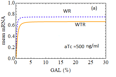
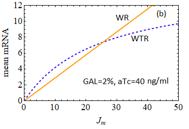
Figure 19: Variation of mean mRNA against GAL keeping aTc = 500 ng ml^-1 as parameter in (a) and mean mRNA vs $J_{m}$ with aTc = 40 ng ml^-1 and GAL = 2% as parameter in (b) while other rate constants are chosen from Blake et al. [3].

Figure 17(a) and figure 19(a) shows that $m^{WR}$ is higher than $m^{WTR}$ keeping GAL and aTc as parameter respectively but figure 19(b) shows a different scenario where we keep both GAL and aTc fixed. It is verified that, the slope of mean mRNA curve becomes high against $J_{m}$ for a higher concentration of GAL keeping aTc fixed. On the other hand, if we increase aTc for a fixed GAL the slope of the curve goes high against $J_{m}.$ Imposing the condition $m^{WR}=m^{WTR}$ we have found a critical value of $J_{m}$ given by

$$J_{m}^{cr}=\frac{k_{3}\left(B_{7}-b_{11}k_{11}\right)-\left(b_{9}+B_{7}\right)k_{r}}{b_{9}+B_{7}}$$ (20)

where, $B_{7}=a_{2}k_{1}k_{5}+a_{4}+b_{11}k_{2}$ and $k_{r}=k_{4}+k_{11}$

other parameters are supplied earlier.

                                    Appendix - E

Model fitting parameters: We proposed an analytical model that fits very much to the experimental data as supplied by Blake et al. [3]. The parameters are chosen from the supplementary material of [3]. The form of parameters $k_{1}$ and $k_{2}$ as functions of GAL are determined from an exact analytical treatment as described in the main text. While for the best estimates of other parameters are revised through trial and error to minimize the sum of squared error (SSE) and the mean square error (MSE). We also show the relative percentile error (RE), in figure 20 (a) and (b) for the fitting of each of the data points, which is given by

$$RE=\frac{y_{a}-y_{e}}{y_{e}}.100\%$$ (21)

where, a stands for analytical and e stands for experimental.

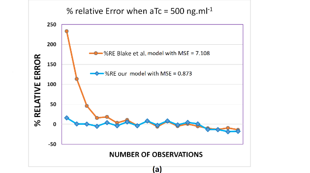
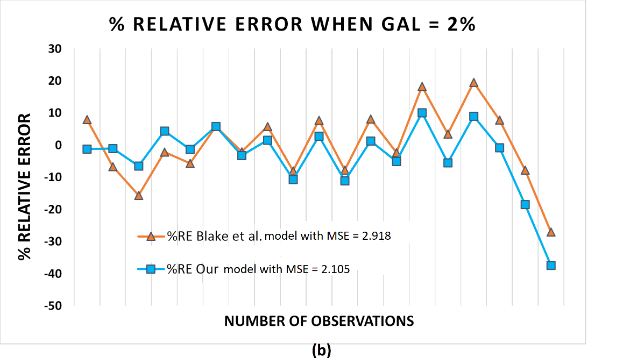
Figure 20: Relative Error for : (a) fitting of curves when aTc is fixed at 500 ng/ml. Blake et al. [3] model offers MSE = 7.108 while our proposed model fits quite nicely with the experimentally observed data with a minimize MSE = 0.873
(b) fitting of curves when aTc is fixed at 500 ng/ml. Blake et al. [3] model offers MSE = 2.918 while our proposed model fits better with the experimentally observed data with a reduced MSE = 2.105

Uncertainty in fitted parameters : The uncertainty of the parameter estimates, is generally expressed by the mean square errors, is proportional to the SSE and inversely proportional to the square of the sensitivity coefficient of the model parameters [58]. The mean square fitting error is

$$\sigma^{2}=\frac{1}{n-k}\sum_{i=1}^{n}(y_{a}-y_{e})^{2}=\frac{Sum\thinspace of\thinspace squared\thinspace error}{(n-k)}$$ (22)

n is the number of observations and k is the number if parameters being determined.

The sensitivity ($\mathscr{S}$) of a function $f(k)$ over the parameter $k$ is given by

$$\mathscr{S}=\frac{k}{f(k)}.\frac{\partial f(k)}{\partial k}$$ (23)

We obtain the sensitivity of the Fano factor (protein) over the fitting parameters and calculate MSE of each parameter keeping others as constant.

$$MSE=\frac{\sigma^{2}}{\sum_{i=1}^{n}[\frac{\partial f(k)}{\partial k}]^{2}}$$ (24)

where the denominator is the coefficient of sensitivity, squared and summed over all observations.

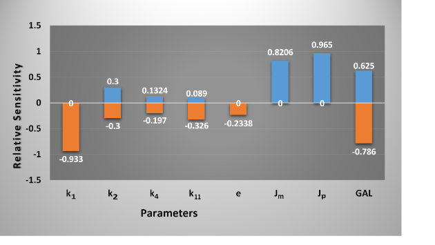
Figure 21: Relative Sensitivity of the Fano factor as functions of fitting parameters

The GAL is the most sensitive parameter and e is the least in order. We found that, the Fano factor is sensitive within a small range of values of these parameters and with the best parameter estimation and minimization of errors (see figure 22) support the robustness of our result. The square root of the MSE is the standard deviation, and the approximate 95% confidence interval for k is [58]

$$[k]_{95\%}=\kappa\pm 2\surd MSE$$ (25)

$\kappa$ is the best estimate value of parameter $k.$

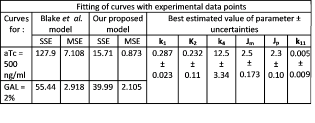
Figure 22: Table for the errors in curve fitting, estimated parameter values and their uncertainties.

Acknowledgment

The author would like to acknowledge the helpful suggestions of Dr. Rajesh Karmakar during the initial stage of the project, before he deceased on 09th June 2021. The author also thanks Dr. Indrani Bose and Dr. Arindam Lala for their valuable suggestions and discussions on the paper.

Glossary

• Transcription factor : Transcription factors (TFs) are proteins which have DNA binding domains with the ability to bind to the specific sequences of DNA (called promoter). They controls the rate of transcription. If they enhance transcription they are called activators and termed as repressors if inhibit transcription.

• Fano factor and Noise strength : The Fano factor is the measure of deviations of noise from the Poissonian behavior and is defined as [50, 51] ,

$$Fano\thinspace factor=\frac{variance}{mean}=\frac{(standard\thinspace deviation)^{2}}{mean}$$

So, for a given mean, smaller the Fano factor implies smaller variance and thus less noise. Therefore, the Fano factor gives a measure of noise strength which is defined (mathematically) as [2],

$$noise\thinspace strength=\frac{variance}{mean}=\frac{(standard\thinspace deviation)^{2}}{mean}$$

• Transcriptional efficiency : Transcriptional efficiency is the ratio of instantaneous transcription to the maximum transcription.

References

- [1] M. B. Elowitz, A. J. Levine, E. D. Siggia and P. S. Swain, “Stochastic gene expression in a single cell”, Science 297 1183 (2002).
- [2] E. M. Ozbudak, M. Thattai, I. Kurtser, A. D. Grossman and A. V. Oudenaarden, “Regulation of noise in the expression of single gene”, Nature Genet. 31 69 (2002).
- [3] W. J. Blake, M. Kaern, C. R. Cantor and J. J. Collins, “Noise in eukaryotic gene expression”, Nature 422 633 (2003).
- [4] J. M. Raser and E. K. O’Shea, “Noise in gene expression: origins, consequences, and control”, Science 309 2010 (2005).
- [5] I. Golding, J. Paulsson, S. M. Zawilski and E. C. Cox, “Real-time kinetics of gene activity in individual bacteria”, Cell 123 1025 (2005).
- [6] W. J. Blake, G. Balazsi, M. A. Kohanski, F. J. Isaas, K. F. Murphy, Y. Kuang, C. R. Cantor, D. R.Walt and J. J. Collins, “Phenotypic consequences of promoter-mediated transcriptional noise”, Molecular Cell 24 853 (2006).
- [7] A. Raj, C. S. Peskin, D. Tranchina, D. Y. Vargas and S. Tyagi, “Stochastic mRNA synthesis in mammalian cells”, PLOS Biol. 4 e309/1707 (2006).
- [8] D. M. Suter, M. Molina, D. Gatfield, K. Schneider, U. Schibler and F. Naef, “Mammalian genes are transcribed with widely different bursting kinetics”, Science 332 472 (2011).
- [9] C. R. Bartman, N. Hamagami, C. A. Keller, B. Giardine, R. C. Hardison, G. A. Blobel and A. Raj, “Transcriptional burst initiation and polymerase pause release are key control points of transcriptional regulation”, Molecular Cell 79 519 (2019).
- [10] F. M. V. Rossi, A. M. Kringstein, A. Spicher, O. M. Guicherit and H. M. Blau, “Transcriptional Control: Rheostat Converted to On/Off Switch”, Molecular Cell 6 723 (2000).
- [11] S. R. Biggar and G. R. Crabtree, “Cell signaling can direct either binary or graded transcriptional responses”, EMBO J. 20 3167 (2001).
- [12] J. Paulsson, “Models of stochastic gene expression”, Physics of Life Review 2 157 (2005).
- [13] A. Sanchez and J. Kondev, “Transcriptional control of noise in gene expression”, PNAS 105 5081 (2008).
- [14] V. Shahrezaei and P. S. Swain, “Analytical distributions for stochastic gene expression”, PNAS 105 17256 (2008).
- [15] R. Karmakar and I. Bose, “Graded and binary responses in stochastic gene expression”, Phys. Biol. 1 197 (2004).
- [16] R. Karmakar, “Conversion of graded to binary responses in an activator-repressor system”, Phys. Rev. E. 81 021905 (2010).
- [17] N. Kumar, T. Platini and R. V. Kulkarni, “Exact distribution for stochastic gene expression models with bursting and feedback”, Phys. Rev. Lett. 113 268105/1 (2014).
- [18] M. Ptashne, “Regulation of transcription: from lambda to eukaryotes”, TRENDS in biochemical Sciences 30 275 (2005).
- [19] D. Zenklusen, D. R. Larson and R. H. Singer, “Single-RNA counting reveals alternate modes of gene expression in yeast”, Nat. Struc. & Mol. Biol. 15 1263 (2008).
- [20] A. J. M. Larson, P. Johnsson, M. H. Jensen, L. Hartmanis, O. R. Faridani, B. Reinius, A. Segerstolpe, C. M. Rivera, B. Ren, R. Sandberg, “Genomic encoding of transcriptional burst kinetics”, Nature 565 251 (2019).
- [21] S. Chong, C. Chen, H. Ge and X. S. Xie, “Mechanism of transcriptional bursting in bacteria”, Cell 156 1274 (2014).
- [22] J. R. Chubb, T. Treck, S. M. Shenoy and R. H. Singer, “Transcriptional Pulsing of a developmental gene”, Current Biology 16 1018 (2006).
- [23] W. Shao and J. Zeitlinger, “Paused RNA Polymerase II inhibits new transcriptional initiation”, Nat. Genetics ADVANCE ONLINE PUBLICATION doi: 10.1038/ng.3867 (2017).
- [24] N. Yudkovsky, J. A. Ranish and S. Hahn, “A transcription reinitiation intermediate that is stabilized by activator”, Nature 408 225 (2000).
- [25] C. R. Bratman, N. Hamagami, C. A. Keller, B. Giardine, R. C. Hardison, G. A. Blobel and A. Raj, “Transcriptional burst initiation and polymerase pause release are key control points of transcriptional regulation”, Molecular Cell 73 519 (2019).
- [26] R. Karmakar, “Control of noise in gene expression by transcriptional reinitiation”, Journal of Statistical Mechanics: Theory and Experiment 20 063402 (2020).
- [27] Z. Cao, T. Filatova, D. A. Oyarzun and R. Grima, “A stochastic model of gene expression with polymerase recruitment and pause release”, Biophysical J. 119 1002 (2020).
- [28] R. Karmakar R. and A. K. Das, “Effect of transcription reinitiation in stochastic gene expression”, Journal of Statistical Mechanics: Theory and Experiment 21 033502 (2021).
- [29] B. Alberts, A. Johnson, J. Lewis, M. Raff, K. Roberts and P. Walters, “Molecular Biology of the Cell” (UK : Garland Science) (2002).
- [30] A. Barberis and M. Petrascheck, “Transcription activation in eukaryotic cells”, Encyclopedia of life sciences doi:10.1038/npg.els.0003303 (2003).
- [31] K. Struhl, “Fundamentally different logic of gene regulation in eukaryotes and prokaryotes”, Cell 98 1-4 (1999).
- [32] N. G. van Kampen, “Stochastic Processes in Physics and Chemistry”, (North-Holland, Amsterdam) (1985).
- [33] D. T. Gillespie, “Exact stochastic simulation of Coupled Chemical Reactions”, J. Phys. Chem. 81 2340-2361 (1977).
- [34] B. Liu, Z. Yuan, K. Aihara and L. Chen, “Reinitiation enhances reliable transcriptional responses in eukaryotes”, J. R. Soc. Interface 11 0326/1-11 (2014).
- [35] H. Maamar, A. RaJ and D. Dubnau, “Noise in Gene Expression Determines Cell Fate in Bacillus subtilis”, Science 317 526-529 (2007).
- [36] M. Acar, J. T. Mettetal and A. van. Oudenaarden, “Stochastic switching as a survival strategy in fluctuating environments”, Nat. Genet. 40 471-475 (2008).
- [37] J. A. Magee, S. A. Abdulkadir and J. Milbrandt, “Haploinsufficiency at the Nkx 3.1 locus. A paradigm for stochastic, dose-sensitive gene regulation during tumor initiation”, Cancer Cell 3 273-283 (2003).
- [38] L.S. Weinberger, J. C. Burnett, J. E. Toettcher, Arkin A. P. and Schaffer D. V., “Stochastic Gene Expression in a Lentiviral Positive-Feedback Loop: HIV-1 Tat Fluctuations Drive Phenotypic Diversity”,Cell 122 169-182 (2005).
- [39] M. Kaern, T.C. Elston, W. J. Blake and Collins J. J., “Stochasticity in gene expression: from theories to phenotypes”, Nat. Rev. Genet 6 451-464 (2005).
- [40] A. Raj and A. van. Oudenaarden, “Nature, nurture, or chance: Stochastic gene expression and its consequences”, Cell 135 723-728 (2008).
- [41] A. Sanchez, S. Choubey and J. Kondev, “Regulation of Noise in Gene Expression”, Annu. Rev. Biophys 42 469-491 (2013).
- [42] L. Bintu, et al., “Transcriptional regulation by the numbers: Models”, Curr Opin Genet Dev 15 116-124 (2005).
- [43] L. Bintu, et al., “Transcriptional regulation by the numbers: Applications”, Curr Opin Genet Dev 15 125-135 (2005).
- [44] T. Kuhlman, Z. Zhang, M. H. Saier, Jr., T. Hwa, “Combinatorial transcriptional control of the lactose operon of Escherichia coli”, Proc Natl Acad Sci USA 104 6043-6048 (2007).
- [45] J. M. G. Vilar, L. Saiz, “DNA looping and physical constraints on transcription regulation”, J Mol Biol 331 981-989 (2003).
- [46] J. M. G. Vilar, L. Saiz, “DNA looping in gene regulation: From the assembly of macromolecular complexes to the control of transcriptional noise”, Curr Opin Genet Dev 15 136-144 (2005).
- [47] T. B. Kepler, T. C. Elston, “Stochasticity in transcriptional regulation: Origins, consequences, and mathematical representations”, Biophys J 81 3116-3136 (2001).
- [48] Y. Setty, A. E. Mayo, M. G. Surette, U. Alon, “Detailed map of a cis-regulatory input function”, Proc Natl Acad Sci USA 100 7702-7707 (2003).
- [49] K. F. Murphy, G. Balazsi, J. J. Collins, “Combinatorial promoter design for engineering noisy gene expression”, Proc Natl Acad Sci USA 104 12726-12731 (2007).
- [50] S. Braichenko, J. Holehouse, R. Grima, “Distinguishing between models of mammalian gene expression: telegraph-like models versus mechanistic models”, Interface 18 20210510 (2021).
- [51] A. Raj, A. V. Oudenaarden, “Single-molecule approaches to stochastic gene expression”, Annu. Rev. Biophys 38 255-270 (2009).
- [52] M. Gossen, H. Bujard, “Anhydrotetracycline, a novel effector for tetracycline controlled gene expression systems in eukaryotic cells”, Nucleic acids research 21(18) 4411-4412. https://doi.org/10.1093/nar/21.18.4411 (1993).
- [53] F. Jiao, C. Zhu, “Regulation of Gene Activation by Competitive Cross Talking Pathways”, Biophysical journal 119(6) 1204-1214. https://doi.org/10.1016/j.bpj.2020.08.011 (2020).
- [54] A. K. Das, work in progress on a “competitive binding of activator-repressor system”, (2021-2022).
- [55] F. M. Rossi, A. M. Kringstein, A. Spicher, O.M. Guicherit, H. M. Blau, “Transcriptional control: rheostat converted to on/off switch”, Molecular cell 6(3) 723-728 (2000).
- [56] R. D. Dar, N. N. Hosmane, M. R. Arkin, R. F. Siliciano, L. S. Weinberger, “Screening for noise in gene expression identifies drug synergies”, Science (New York, N.Y.) 344(6190) 1392–1396 (2014).
- [57] T. Dingermann, U. Frank-Stoll, H. Werner, A. Wissmann, W. Hillen, M. Jacquet, & R. Marschalek, “RNA polymerase III catalysed transcription can be regulated in Saccharomyces cerevisiae by the bacterial tetracycline repressor-operator system”, The EMBO journal 11(4) 1487-1492 (1992).
- [58] L. H. Smith, P. K. Kitanidis, and P. L. McCarty, “Numerical modeling and uncertainties in rate coefficients for methane utilization and TCE co-metabolism by a methane-oxidizing mixed culture”, Biotechnol. Bioeng. 53 320–331 (1997).