Concerning the stability of biexcitons in hybrid HJ aggregates of $\pi$-conjugated polymers

Abstract

Frenkel excitons are the primary photoexcitations in organic semiconductors and are ultimately responsible for the optical properties of such materials. They are also predicted to form bound exciton pairs, termed biexcitons, which are consequential intermediates in a wide range of photophysical processes. Generally, we think of bound states as arising from an attractive interaction. However, here we report on our recent theoretical analysis predicting the formation of stable biexciton states in a conjugated polymer material arising from both attractive and repulsive interactions. We show that in J-aggregate systems, 2J-biexcitons can arise from repulsive dipolar interactions with energies $E_{2J}>2E_{J}$ while in H-aggregates, 2H-biexciton states $E_{2H}<2E_{H}$ corresponding to attractive dipole exciton/exciton interactions. These predictions are corroborated by using ultrafast double-quantum coherence spectroscopy on a PBTTT material that exhibits both J- and H-like excitonic behavior.

I Introduction

It is generally understood that the primary photoexcitations in organic semiconducting materials are molecular $\pi-\pi^{*}$ electronic singlet states (S_1) termed Frenkel excitons [1]. While local in nature, at sufficiently high packing densities, excitons can delocalized over several molecular units and sufficiently higher excitation densities, exciton-exciton interactions begin to dominate the optical properties of such materials [2]. Biexcitons, bound pairs of excitons, are consequential intermediates in a wide range of photophysical processes such as exciton dissociation into electrons (e^-) and holes (h⁺)  [3],

$$\ce{S0+2$\hbar\omega$->[2S1]$^{\ddagger}$->2e^{-}+2h^{+}}$$ (1)

bimolecular annihilation [4],

$$\ce{S1+S1->[2S1]$^{\ddagger}$->S0+S0}$$ (2)

and singlet fission producing triplet (T1) states  [5]

$$\ce{S0+2$\hbar\omega$->[2S1]$^{\ddagger}$->T1+T1}.$$ (3)

Ref. 4 notes that bimolecular annihilation may be mediated both by resonance energy transfer and diffusion-limited exciton-exciton scattering, but in either case we invoke the key intermediate [2 S1]^‡. Examples of this occur in biological light harvesting complexes where multi-exciton interactions may play important roles [6] in the excitonic transport process,and biexcitons can be crucial in cascade quantum emitters as a source of entangled photons [7]. While ample theoretical work points towards the existence of biexcitons in organic solids [8, 9, 10, 11, 12, 13, 14], and in optical lattices [15], there has been only indirect evidence of the dynamic formation of two-quantum exciton bound states in polymeric semiconductors by incoherent, sequential ultrafast excitation [3, 4, 5, 16, 17].

Recently, we reported upon the the direct spectroscopic observation of bound Frenkel biexcitons, i.e., bound two-exciton quasiparticles ([2S1]^‡), in a model polymeric semiconductor, [poly(2,5-bis(3-hexadecylthiophene-2-yl)thieno[3,2-b]thiophene)] [18] (PBTTT) using coherent two-dimensional ultrafast spectroscopy. [19] The chemical structure of PBTTT is given in Fig. 1(A). PBTTT is unique in that depending upon processing conditions, it can support the formation of both H and J aggregate single exciton states, suggesting an arrangement as sketched in Fig1(B) in which intra-chain J-like excitons can form along the chains spanning over several PBTTT subunits, while inter-chain H-like excitons can form due to parallel stacking of several chains within the aggregate. The experimental observations revealed a correlation between peaks in the single and double quantum spectra the correspond to the formation of 2H and 2J biexciton species. This conclusion was supported by both a computational model and theoretical analysis based upon a quasi-one-dimensional continuum model.

Here present an overview of the theoretical model we developed for biexcitons and use it to discuss biexcitons in related organic polymer materials. First, we show how one can reduce the two-dimension lattice problem into two separate one-dimensional problems and use a Greens function approach to account for the contact interaction between excitons. This gives the criterion for the overall stability of the bound biexciton states in terms of the exciton band-width and contact interaction. Formally, the lattice model reduces to a one-dimensional continuum model with $\delta$-function potential. We append to this “text-book” model a deformable classical media to examine the contribution of the lattice reorganization about the bound-biexciton states and find that this stabilizes the attractively bound biexciton state but destabilizes the repulsively bound states. We conclude by discussing the experimental observations and the need for a better theoretical understanding of bound biexciton states.

Figure 1: (a) Chemical structure of the PBTTT polymer. (b) Local packing of excitonic units (ellipsoids) with superimposed transition dipoles (yellow arrows) with J-like interactions along the horizontal axis and H-like interactions along the vertical axis.

II Theoretical model

II.1 Homogeneous lattice model in 1- and 2-dimensions

To explore the possibility of having multiple species of bound, biexcitons in the same system, we begin by writing a generic lattice model for the system by defining exciton operators $a_{\textbf{n}}$ and $a_{\textbf{n}}^{\dagger}$

$$a_{\textbf{n}}a_{\textbf{m}}^{\dagger}-(-1)^{\delta_{\textbf{nm}}}a_{\textbf{m}}^{\dagger}a_{\textbf{n}}=\delta_{\textbf{nm}}.$$ (4)

These operators are Paulion operators that create and remove single excitations on to a site labeled by n. On a given site, they obey the Fermion relation $a_{\textbf{n}}a_{\textbf{n}}^{\dagger}+a_{n}^{\dagger}a_{n}=1$ which enforces Pauli exclusion since $a_{n}a_{n}=a_{n}^{\dagger}a_{n}^{\dagger}=1$, but commute “off-site” with $[a_{\textbf{n}},a_{\textbf{m}}^{\dagger}]=0$ when $\textbf{n}\neq\textbf{m}$. This is different than the usual Fermion algebra where the anti-commutation rule is applies over all sites, ultimately giving rise to the exchange interaction. Further, we can write a generic multi-exciton Hamiltonian as

$$H=\sum_{\textbf{nm}}h_{\textbf{nm}}a_{\textbf{n}}^{\dagger}a_{\textbf{m}}+\frac{1}{2}\sum_{\textbf{nm}}U_{\textbf{nm}}a^{\dagger}_{\textbf{n}}a^{\dagger}_{\textbf{m}}a_{\textbf{n}}a_{\textbf{m}}.$$ (5)

where $h_{\textbf{nm}}$ describes the single-exciton dynamics and $U_{\textbf{nm}}$ is the exciton/exciton interaction. In principle, the parameters entering into the Hamiltonian in Eq. 5 are defined by the system of interest. For the case of excitons, the diagonal elements of the single particle term defines the energy to place an exciton in site n, and we write $h_{\textbf{n}n}=\epsilon_{n}$. For a homogeneous lattice, all site energies are the same, and $\epsilon_{n}=\epsilon_{o}$. Similarly, the off-diagonal elements of $h_{\textbf{nm}}$ correspond to the matrix elements for transferring an excitation from site $\textbf{n}\to\textbf{m}$. To a good approximation, the single-exciton transfer interaction can be described within the dipole-dipole approximation as described above. This model differs from the Hubbard model commonly studied in condensed matter physics in that we explicitly exclude double occupancy of each lattice and the exciton/exciton interaction is taken to be between occupied neighbors. Formally, a Frenkel exciton corresponds to a single electron/hole excitation on a given site. However, molecules are not point particles and excitons may acquire some intramolecular charge-transfer character. Therefore, we anticipate that $U_{\textbf{nm}}$ is also dipole-dipole like and reflects the relative orientation of the static exciton dipole moments.

For a one-dimensional chain with lattice spacing $a$, $n$ is simply an index along the chain such that the site location is given by $r_{\textbf{n}}=\textbf{n}a$. However, for 2- and 3-dimensional systems, we shall take it as an n-tuple index specifying the site location. For the single particle term, $h_{\textbf{nn}}$ is the excitation energy for single site ($\varepsilon_{\textbf{n}}$) and $h_{\textbf{nm}}$ (for $\textbf{n}\neq\textbf{m}$) corresponds to the hopping integral between sites. Upon transforming into the reciprocal space,

$$\tilde{a}_{\textbf{k}}=\frac{1}{\sqrt{N}}\sum_{\textbf{n}}e^{-\textbf{k}\cdot\textbf{n}}a_{\textbf{n}}$$ (6)

one finds the single particle energy dispersion as

$$(\varepsilon(\textbf{k})-E)e^{i\textbf{k}\cdot\textbf{n}}=\sum_{\textbf{m}}h_{\textbf{nm}}e^{i\textbf{k}\cdot\textbf{m}}.$$ (7)

To determine the 2-exciton states, we begin by writing

$$|\psi\rangle=\sum_{\textbf{kk}^{\prime}}c_{\textbf{kk}^{\prime}}\tilde{a}^{\dagger}_{\textbf{k}}\tilde{a}_{\textbf{k}^{\prime}}^{\dagger}.$$ (8)

where $c_{\textbf{k}\textbf{k}^{\prime}}$ are the expansion coefficients for this state. At this point, there are various approaches one can take to find the general solutions for the Schrödinger equation for the 2-exciton system. Indeed, for a small enough lattice, one can simply directly diagonalize the Hamiltonian in Eq. 5 for a finite sized grid. However, we are not interested the full solution of this problem. Rather, we are focused upon only solutions corresponding to bound exciton pairs, and especially those bound pairs that retain their J- or H-like excitonic character. With this in mind, we develop an analytical solution that naturally extends to the full model.

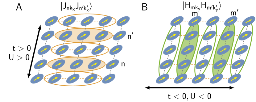
Figure 2: Sketch of 2D lattice model with superimposed transition dipole for each site. In (A), we define a J-aggregate basis and create 2J biexciton configurations along each row. In (B), we define an H-aggregate basis along each column. As discussed in the text, these are equivalent representations of the full 2D problem and are useful for reducing the 2D problem into two separate (but formally identical) 1D problems.

II.2 Local exciton approximation

In Ref.  19 employed both direct diagonalization and a lattice Greens function approach developed by Vektaris[9] to study the properties of the biexciton including its dispersion and the affects of local disorder. A key assumption in our model is that we can define two equivalent quasi-one-dimensional representations for H-like or J-like excitons. For this, let us define a new set of exciton operators, $\hat{J}^{\dagger}_{k_{x}}(n)$ and $\hat{J}_{k_{x}}(n)$ which creates or removes an exciton with wavevector $k_{x}$ in the $x$-direction localized on the $n$th row of sites. Similarly, we define operators $\hat{H}_{k_{y}}^{\dagger}(m)$ and $\hat{H}_{k_{y}}(m)$ which create and remove excitons with wavevector $k_{y}$ in the $y$-direction, but localized to the $m$th column, as sketched in Fig. 2. These can be written in terms of the original lattice operators

$$\hat{J}_{m,k_{x}}=\frac{1}{\sqrt{N}}\sum_{n}e^{ik_{x}n}a_{(n,m)}$$ (9)

$$\hat{H}_{n,k_{y}}=\frac{1}{\sqrt{N}}\sum_{m}e^{ik_{y}m}a_{(n,m)}.$$ (10)

Both are equivalent representations and we can choose to use either (but not both) to rewrite the original problem in this new representation.

Thus, we can write

$$\sum_{\textbf{nm}}h_{\textbf{nm}}a^{\dagger}_{\bf n}a_{\bf m} =\sum_{k_{x}mm^{\prime}}(\varepsilon_{J}(k_{x})\delta_{mm^{\prime}}+t_{H}(mm^{\prime})\hat{J}^{\dagger}_{m,k_{x}}\hat{J}_{m^{\prime},k_{x}}$$

$$=\sum_{k_{y}nn^{\prime}}(\varepsilon_{H}(k_{y})\delta_{nn^{\prime}}+t_{J}(nn^{\prime}))\hat{H}^{\dagger}_{n,k_{y}}\hat{H}_{n^{\prime}k_{y}}$$ (11)

where in the first line we diagonalized in the J-direction and in the second, we diagonalized in the H-direction. This implies that we can think of a J-exciton state as moving in the H-direction with hopping integral $t_{H}$ and H-exciton states as moving in the J-direction with hopping integrals $t_{J}$. The dispersion relations are then as usual

$$\varepsilon_{J}(k_{x}) =\epsilon_{0}+2t_{J}\cos(k_{x})$$ (12)

$$\varepsilon_{H}(k_{y}) =\epsilon_{0}+2t_{H}\cos(k_{y})$$ (13)

where $t_{J}<0$ is the nearest-neighbor coupling along the $x$-direction and $t_{H}>0$ is the nearest-neighbor coupling taken in the $y$-direction. To remind, throughout we are taking the wavevector $k\in[-\pi,\pi]$. Since the problem is formally separable between $x$ and $y$ directions, the single-particle terms do not mix wavevector components since $k_{x}$ and $k_{y}$ are “good” quantum numbers for this system. Using the $\hat{J}$ and $\hat{H}$ operators, we can reduce the 2-particle/2-dimensional problem into a one for pair of particles within a 1 dimensional frame without loss of generality.

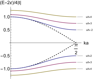
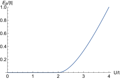
Figure 3: (a) Energy bands for attractive (2H) and repulsively (2J) bound biexcitons. Dashed lines correspond to the non-interacting $U\to 0$ limit of the model. Solid curves are plotted for the case of $U/2t>1$ as indicated. The dispersion curves need to be taken at the corresponding points in $k$-space with a corresponding shift in the energy origins for each exciton species. (b)Variation in the biexciton binding energy at $k=0$ with increasing exciton/exciton interactions.

This decomposition suggest that motion in one direction can be very different than motion in the perpendicular direction due to the orientations of the transition dipoles between neighboring units. In Fig. 1(B) we suggest how this can be accomplished within the context of molecular aggregates with $\pi$- stacking. Here, excitonic sites are denoted as blue ellipsoids along with their respective local transition dipole moments (yellow arrows). Along the $x$-direction of the 2-dimensional lattice sketched here, the transition moments are oriented more or less in a “head-to-tail” arrangement producing a hopping matrix element in $h_{\textbf{nm}}<0$. In the $y$-direction, however, the transitions moments are aligned co-facially producing a single-particle hopping matrix element $h_{\textbf{nm}}>0$. In the former case, the optically bright state occurs at the bottom of the energy band (J-aggregate), whilst in the latter case the optically bright state occurs at the top of the energy band (H-aggregate). The PBTTT material is unique in that both J- and H- aggregate states can be readily observed, depending upon the sample preparation.

If we use the $J_{km}$ (or $H_{kn}$) states as a basis for a given value of $k$, we can use the Greens function approach to find the biexciton energies as

$$E_{XX}(k)=2\varepsilon_{x}+\frac{4t^{2}}{U}\cos^{2}(k)+U$$ (14)

where $\epsilon_{x}$ is the excitation energy of either the $J$ or $H$ single exciton and $U$ is the contact interaction. [9] This expression is predicated upon $|U/2t|>1$ in order for the the biexciton wavefunction to decay exponentially with exciton-exciton separation. These dispersions are plotted in Fig. 3a for both 2H and 2J biexcitons. In each case, the energy origin should be shifted to twice the J or H exciton energy. At $k=0$, the difference between the interacting and localized excitons is the contact energy $U$, which defines the binding energy for the exciton pair. The binding energy must be at least greater in magnitude than $4t$, else the lowest energy interacting state will be still within the band for the freely dissociated pairs. These bands will split from the freely dissociated bands once $U/2t>1$.

II.3 Optical Transitions

It is important to keep in mind that two types of excitons sketched in Fig.1 occur at different wave-vectors. In Fig.1(a) the J-like exciton has its longest wavelength in the $x$-direction (corresponding to $k_{x}=0$) while having the shortest possible wavelength in the $y$-direction (i.e. $k_{y}=\pm\pi/a$). Transitions to this state from the exciton vacuum (ground states) are allowed under the dipole approximation for the transition moment. Consequently, double excitations can create either pairs of free J-like excitons or bound 2J excitons. Similarly, optically allowed H-like single excitons are delocalized along the $y$-direction but localized along the $x$-direction (i.e. ${\bf k}=\{\pm\pi/a,0\}$) implying that the double excitations must also occur at these wave-vectors. Bearing this in mind, the dispersion curves plotted in Fig. 3 need to be taken at the corresponding points in $k$-space with a corresponding shift in the energy origins for each exciton species.

II.4 Biexciton stability

According to our model, Frenkel biexcitons mix J-like and H-like character in terms of their collective quantum behavior with the requirement that the ratio of the exciton/exciton interaction and the perpendicular hopping term be $U/t>0$ which gives rise to localized biexciton states in the perpendicular direction. For the 1D $\delta$-function potential, any attractive interaction with $U/t>0$ produces a localized state with localization length $\lambda=\kappa^{-1}=2t/U$. For the 1D lattice, bound biexciton states occur outside the band for free biexcitons. To gain further insight into the stability of these states, we turn to a continuum model and work in a relative coordinate reference frame where $x=|r_{1}-r_{2}|$ is the separation between two localized excitons. Thus, the biexciton Schrödinger equation can be approximated as

$$t\psi^{\prime\prime}+U\delta(x)\psi=E\psi$$ (15)

where $U$ is the contact interaction between the two excitons. For bound states, $\psi(x)$ must vanish as $x\to\pm\infty$, giving that

$$\psi(x)=\left\{\begin{array}[]{cc}\sqrt{\kappa}e^{-\kappa x}&x>0\\ \sqrt{\kappa}e^{+\kappa x}&x<0\end{array}\right.$$ (18)

where $\kappa=U/2t$ is a positive constant and $E=t\kappa^{2}$. In general, we take $t=-\hbar^{2}/2\mu_{eff}$ and $U<0$ for an attractive potential giving rise to a bound state energetically below the continuum for the scattering states.

II.4.1 Lattice reorganization in the impurity model

Generally speaking, one cannot discount the role of lattice reorganization and relaxation when discussing excitons and biexcitons in organic polymer semiconducting systems. To study this, we append to the 1D impurity model a continuum model for the medium a term coupling the biexciton to the lattice as per the Davydov model. [21, 22, 23, 24, 25, 26, 27, 28, 29, 30] The resulting equations of motion read

$$i\hbar\dot{\psi}(x) =(t\nabla^{2}+U\delta(x)+(E_{o}+2\chi\nabla u(x)))\psi(x)$$

$$\ddot{u}-\frac{k}{m}\nabla^{2}u =2\frac{\chi}{m}\nabla|\psi|^{2}$$ (19)

where $u(x)$ is the lattice deformation, $\chi$ describes the linear coupling between the biexciton and the lattice, $m$ is the mass of the lattice “atoms” and $k$ is the elastic modulus. If we seek traveling wave solutions, $u(x,t)=u(x-vt)$ where $v$ is the group velocity, we find a closure relation

$$\nabla u=-\frac{2\chi}{k(1-(v/c)^{2})}|\psi|^{2}$$ (20)

that gives us a non-linear Schrödinger equation

$$i\hbar\dot{\psi}=(t\nabla^{2}+g|\psi|^{2}+U\delta(x))\psi$$ (21)

where $g=-4\chi^{2}/(k(1-(v/c)^{2}))$ and $c$ is the sound velocity. Note that $E_{o}$ is a constant given by

$$E_{o}=E-2t+\frac{1}{2}\int_{-\infty}^{\infty}\left(m\ddot{u}^{2}+ku^{\prime\prime}\right)dx.$$ (22)

that we can ignore for purposes of this analysis. The $\delta$-function potential implies the wave function should have the form in Eq. 18. Taking $\kappa$ as a variational parameter and minimizing the total energy, one obtains

$$\kappa=\frac{U}{2t}+\frac{g}{8t}.$$ (23)

$\kappa>0$ is necessary to produce a localized state and from above $U/t>0$ and $g<0$ from its definition above, we have a stability requirement that if $U>0$ and $t>0$, then $-g<4U$. Solving for the binding energy,

$$E_{B}=\frac{(4U+g)^{2}}{64t}$$ (24)

we obtain a straight-forward estimate of the contribution of both the lattice and the exciton/exciton coupling to the biexciton binding.

In Fig. 4 we plot the biexciton binding energy versus the non-linearity parameter, $g$. For the attractively bound 2H, lattice reorganization is expected to stabilize the biexciton state by further localizing the state ($\kappa$ increases as $g$ increases in magnitude). On the other hand, for the 2J state, increasing the magnitude of $g$ decreases $\kappa$ and destabilizes the otherwise bound 2J state. When $-g=2U$ the state is fully delocalized and further increases in the lattice coupling lead to unbound solutions.

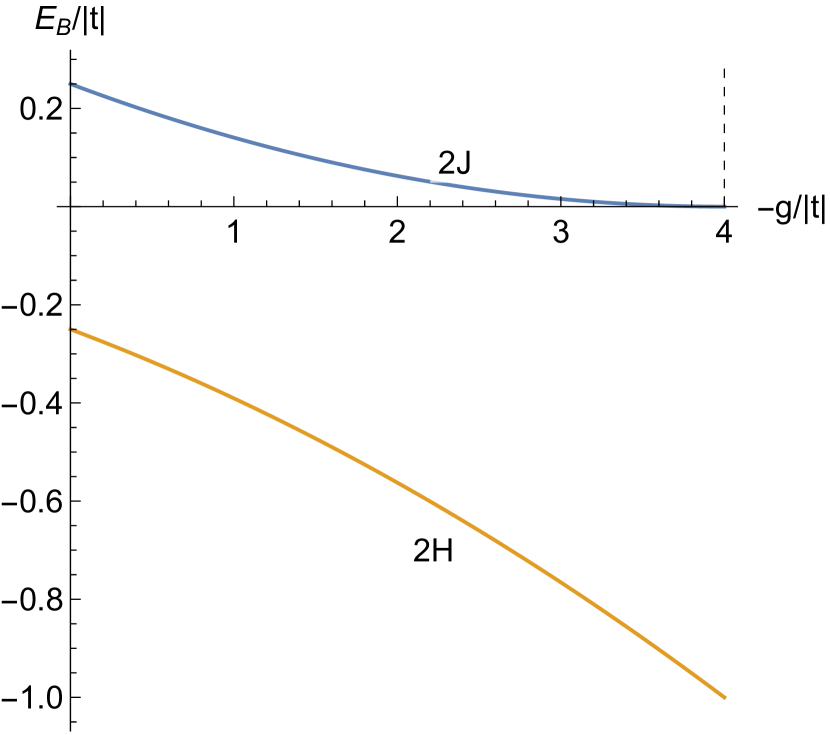
Figure 4: Biexciton binding energy (in reduced units) for the 2J and 2H cases versus increasing exciton/lattice coupling. For the attractively bound 2H, lattice reorganization is expected to stabilize the biexciton state while destabilizing the 2J. The dashed line indicates the limit of stability for the 2J case.

III Comparison to experimental measurement

We have examined the theoretical concepts by means of two-dimensional coherent excitation spectroscopy on PBTTT, with structure depicted in Fig. 1(A), which we reported extensively in Ref. 19. In that work, we identified spectral features associated with the 0–0 excitation peak of both the H- and J-aggregate components of the hybrid aggregate, with cross peaks reflecting spectral correlations due to their shared ground state. The origin of the H-aggregate vibronic progression was centered at 2.06 eV, while a weaker peak at 1.99 eV was assigned to the J-aggregate vibronic origin. By performing two-quantum coherence measurements, we found spectral signatures of both 2H and 2J biexcitons. A cross-section of the 2D spectral data along the two-quantum energy axis ($\hbar\omega_{2Q}-\hbar\omega_{diag}$) relative to the two-quantum diagonal ($\omega_{diag}\equiv\omega_{2Q}=2\omega_{1Q}$) is shown in Fig. 5. We found that 2H biexcitons displayed attractive biexciton binding with energy $-64\pm 6$ meV, where as 2J biexcitons displayed repulsive correlations with binding energy $+106\pm 6$ meV; that is that the energy of the 2H-biexciton resonance is lower than twice the H-aggregate resonance energy, while the corresponding energy for the 2J-biexciton resonance is higher.

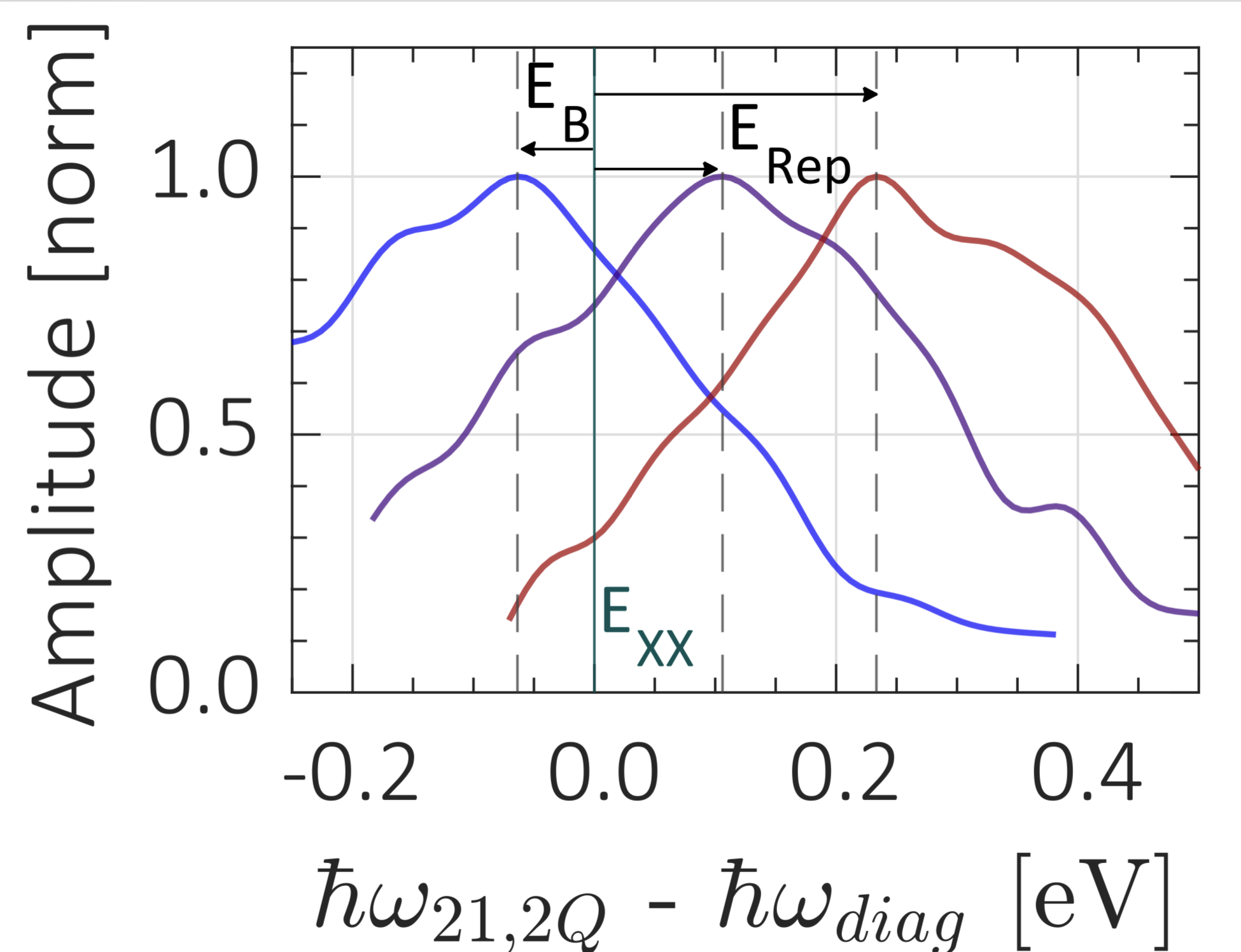
Figure 5: Spectral cuts along the two-quantum coherence energy axis, relative to the two-quantum diagonal energy axis ($\hbar\omega_{2Q}=2\hbar\omega_{1Q}$, $E_{XX}$) at fixed $\hbar\omega_{43}=2.06$ (H-aggregate resonance, blue), $1.99$ (J-aggregate resonance, purple), and $1.94$ eV (J-aggregate resonance, red). Figure from Ref.19

We rationalized this observation as depicted in Fig. 1: two quantum interactions for excitons dispersed along the polymer backbone (J aggregates) are with $J<0$, while $J>0$ for those for between excitons dispersed on several chains (H aggregates). Considering physically reasonable parameters, we concluded that biexcitons in PBTTT are stable by the arguments depicted in Fig. 5.

IV Perspective

We present here theoretical and experimental evidence supporting the formation of bound Frenkel biexcitons in a molecular aggregate material. In our theoretical analysis, we solved the full 2D interacting model and give the conditions necessary for the formation of stable, stationary states corresponding to bound exciton pairs. The model provides a road-map for developing a bi-exciton materials genome in terms of the properties of the J- and H-excitons. We show that for bound biexcitons, both the exciton-exciton interaction $U$ and the single-particle hopping integral $t$ must have the same sign. Furthermore, $U/t>2$ so that the exciton/exciton potential interaction is greater than their total kinetic energy. Curiously, we find that while H-like excitons form bound biexcitons with attractive interactions, J-like exciton pairs form bound states arising from a repulsive interaction. Curiously, we find that while the 2H biexciton is stabilized by interactions with the lattice phonons, the 2J biexciton is destabilized to the extent that strong lattice/exciton interactions will produce only unbound biexciton states, which certainly complicates the observation of these states in systems with strong exciton/phonon coupling. Nonetheless, the 2J biexciton is clearly apparent in the 2D two-quantum experiments in Ref.19.

An open question, however, is the nature of the exciton-exciton interaction itself. Here, we introduce it as a parameter into our model with a dipole-dipole like form in that the exciton-exciton coupling in one direction is different from that in a perpendicular direction. It is also important to point out that while this interaction appears to have a dipole-like form, it necessarily must reflect the static dipole of the local Frenkel excitons rather than their transition dipole moments, which are responsible for the single exciton transfer between local sites. Computing these interactions from a first-principle ab initio theory remains a formidable challenge since it necessitates the accurate calculation of doubly excited states with some degree of charge-separation.

Author Declaration: Both authors contributed equally to the design and analysis of this study. Theoretical methodology was developed by ERB and experiments were designed and analyzed by CS. The manuscript was written and edited by ERB. Both authors have read and agreed to the published version of the manuscript. The authors have no conflicts to disclose.

Data Availability:The data that supports the findings of this study are available within the article.

References

- Frenkel [1931] J. Frenkel, “On the transformation of light into heat in solids. i,” Phys. Rev. 37, 17 (1931).
- Agranovich and Toshich [1968] V. Agranovich and B. Toshich, “Collective properties of frenkel excitons,” Sov. Phys. JETP 26, 104–112 (1968).
- Silva et al. [2001] C. Silva, A. S. Dhoot, D. M. Russell, M. A. Stevens, A. C. Arias, J. D. MacKenzie, N. C. Greenham, R. H. Friend, S. Setayesh, and K. Müllen, “Efficient exciton dissociation via two-step photoexcitation in polymeric semiconductors,” Phys. Rev. B 64, 125211 (2001).
- Stevens et al. [2001] M. A. Stevens, C. Silva, D. M. Russell, and R. H. Friend, “Exciton dissociation mechanisms in the polymeric semiconductors poly (9, 9-dioctylfluorene) and poly (9, 9-dioctylfluorene-co-benzothiadiazole),” Phys. Rev. B 63, 165213 (2001).
- Silva et al. [2002] C. Silva, D. M. Russell, A. S. Dhoot, L. M. Herz, C. Daniel, N. C. Greenham, A. C. Arias, S. Setayesh, K. Müllen, and R. H. Friend, “Exciton and polaron dynamics in a step-ladder polymeric semiconductor: the influence of interchain order,” J. Phys.: Condens. Matter 14, 9803 (2002).
- Scholes et al. [2011] G. D. Scholes, G. R. Fleming, A. Olaya-Castro, and R. Van Grondelle, “Lessons from nature about solar light harvesting,” Nat. Chem. 3, 763–774 (2011).
- Avanaki and Schatz [2021] K. N. Avanaki and G. C. Schatz, “Mechanistic understanding of entanglement and heralding in cascade emitters,” J. Chem. Phys. 154, 024304 (2021).
- Spano, Agranovich, and Mukamel [1991] F. C. Spano, V. Agranovich, and S. Mukamel, “Biexciton states and two-photon absorption in molecular monolayers,” J. Chem. Phys. 95, 1400–1409 (1991).
- Vektaris [1994] G. Vektaris, “A new approach to the molecular biexciton theory,” The Journal of Chemical Physics 101, 3031–3040 (1994), https://doi.org/10.1063/1.467616 .
- Guo, Chandross, and Mazumdar [1995] F. Guo, M. Chandross, and S. Mazumdar, “Stable biexcitons in conjugated polymers,” Phys. Rev. Lett. 74, 2086 (1995).
- Gallagher and Spano [1996] F. B. Gallagher and F. C. Spano, “Theory of biexcitons in one-dimensional polymers,” Phys. Rev. B 53, 3790 (1996).
- Mazumdar et al. [1996] S. Mazumdar, F. Guo, K. Meissner, B. Fluegel, and N. Peyghambarian, “Exciton-to-biexciton transition in quasi-one-dimensional organics,” J. Chem. Phys. 104, 9292–9296 (1996).
- Agranovich et al. [2000] V. Agranovich, O. Dubovsky, D. Basko, G. La Rocca, and F. Bassani, “Kinematic frenkel biexcitons,” J. Lumin. 85, 221–232 (2000).
- Kun et al. [2009] G. Kun, X. Shi-Jie, L. Yuan, Y. Sun, L. De-Sheng, and Z. Xian, “Effect of interchain coupling on a biexciton in organic polymers,” Chin. Phys. B 18, 2961 (2009).
- Xiang, Litinskaya, and Krems [2012] P. Xiang, M. Litinskaya, and R. V. Krems, “Tunable exciton interactions in optical lattices with polar molecules,” Phys. Rev. A 85, 061401 (2012).
- Chakrabarti et al. [1998] A. Chakrabarti, A. Schmidt, V. Valencia, B. Fluegel, S. Mazumdar, N. Armstrong, and N. Peyghambarian, “Evidence for exciton-exciton binding in a molecular aggregate,” Phys. Rev. B 57, R4206 (1998).
- Klimov et al. [1998] V. I. Klimov, D. McBranch, N. Barashkov, and J. Ferraris, “Biexcitons in -conjugated oligomers: Intensity-dependent femtosecond transient-absorption study,” Phys. Rev. B 58, 7654 (1998).
- McCulloch et al. [2006] I. McCulloch, M. Heeney, C. Bailey, K. Genevicius, I. MacDonald, M. Shkunov, D. Sparrowe, S. Tierney, R. Wagner, W. Zhang, et al., “Liquid-crystalline semiconducting polymers with high charge-carrier mobility,” Nat. Mater. 5, 328–333 (2006).
- Gutiérrez-Meza et al. [2021] E. Gutiérrez-Meza, R. Malatesta, H. Li, I. Bargigia, A. R. S. Kandada, D. A. Valverde-Chávez, S.-M. Kim, H. Li, N. Stingelin, S. Tretiak, E. R. Bittner, and C. Silva-Acuña, “Frenkel biexcitons in hybrid hj photophysical aggregates,” Science Advances 7, eabi5197 (2021), https://www.science.org/doi/pdf/10.1126/sciadv.abi5197 .
- Note [1] Note, that here carries units of and carries units of so that carries the appropriate units of [length].
- Scott [1992] A. Scott, “Davydov’s soliton,” Physics Reports 217, 1–67 (1992).
- Edler et al. [2004] J. Edler, R. Pfister, V. Pouthier, C. Falvo, and P. Hamm, “Direct observation of self-trapped vibrational states in -helices,” Physical Review Letters 93, 106405 (2004).
- Sun, Luo, and Zhao [2010] J. Sun, B. Luo, and Y. Zhao, “Dynamics of a one-dimensional holstein polaron with the davydov ansätze,” Phys. Rev. B 82, 014305 (2010).
- Goj and Bittner [2011] A. Goj and E. R. Bittner, “Mixed quantum classical simulations of excitons in peptide helices,” The Journal of Chemical Physics 134, 205103 (2011), https://doi.org/10.1063/1.3592155 .
- Goj and Bittner [2010] A. Goj and E. R. Bittner, “Mixed quantum classical simulations of vibrational excitations in peptide helices,” in Frontiers in Optics 2010/Laser Science XXVI (Optical Society of America, 2010) p. LTuC1.
- Georgiev and Glazebrook [2019a] D. D. Georgiev and J. F. Glazebrook, “On the quantum dynamics of davydov solitons in protein -helices,” Physica A: Statistical Mechanics and its Applications 517, 257–269 (2019a).
- Georgiev and Glazebrook [2019b] D. D. Georgiev and J. F. Glazebrook, “Quantum tunneling of davydov solitons through massive barriers,” Chaos, Solitons and Fractals 123, 275–293 (2019b).
- Kerr and Lomdahl [1987] W. C. Kerr and P. S. Lomdahl, “Quantum-mechanical derivation of the equations of motion for davydov solitons,” Phys. Rev. B 35, 3629–3632 (1987).
- Davydov [1977] A. Davydov, “Solitons and energy transfer along protein molecules,” Journal of Theoretical Biology 66, 379–387 (1977).
- Davydov [1973] A. Davydov, “The theory of contraction of proteins under their excitation,” Journal of Theoretical Biology 38, 559–569 (1973).