The macroeconomic cost of climate volatility

Abstract

We study the impact of climate volatility on economic growth exploiting data on 133 countries between 1960 and 2019. We show that the conditional (ex ante) volatility of annual temperatures increased steadily over time, rendering climate conditions less predictable across countries, with important implications for growth. Controlling for concomitant changes in temperatures, a +1${}^{\text{o}}$C increase in temperature volatility causes on average a 0.3 per cent decline in GDP growth and a 0.7 per cent increase in the volatility of GDP. Unlike changes in average temperatures, changes in temperature volatility affect both rich and poor countries.

Keywords: temperature volatility; economic growth; panel VAR.

JEL Classification: C32, E32, Q54.

It is virtually certain that hot extremes have become more frequent and more intense across most land regions since the 1950s.

IPCC Report n.6, August 2021

1 Introduction

Rising temperatures are known to have a negative impact on economic growth, particularly in poor countries. In its last report, the Intergovernmental Panel on Climate Change (IPCC) highlighted another important dimension of climate change: fluctuations in climate conditions became larger over time, with unprecedented swings in temperatures and precipitations affecting an increasing number of geographical regions (Arias et al., 2021). This paper shows that, from an economic perspective, this phenomenon is as important as the underlying change in temperature levels. We use climate data on 133 countries since the 1960s to estimate a panel VAR with stochastic volatility. The model captures the endogenous interactions between temperatures and economic activity and accomodates shocks that can affect both the level and the variability of the underlying series. This framework allows us to estimate the volatility of the residual change in annual temperatures that cannot be forecasted using past data, quantifying the ex-ante ‘temperature risk’ faced by households and firms in a given country at a given point in time. Combined with appropriate identification restrictions, it also allows us to isolate exogenous changes in temperature volatilities and trace their impact on various economic activity indicators. Our analysis yields two main results. The first one is that temperature volatility increased steadily over time, even in regions that were only marginally affected by global warming. The second one is that temperature volatility matters for economic activity. Controlling for temperature levels, a 1${}^{\text{o}}$C increase in volatility causes on average a 0.3 per cent decline in GDP growth and a 0.7 per cent increase in the volatility of the GDP growth rate. In other words, volatile temperatures lead at once to lower and more variable income growth. Volatility shocks affect rich, non-agricultural countries too, and they are not driven by the occurrence of large fluctuations in GDP, temperatures or precipitations. We find that volatility impacts both consumption and investment, and that its effects are larger for the manufacturing and services sectors. Our findings demonstrate that risk plays an important role in the nexus between climate and the economy. Economic agents respond to changes in the expected variability of the environment, and, as in other macro-financial contexts, lower predictability is by itself detrimental for growth. This suggests that climate risk has important ex-ante implications for welfare, and that uncertainty on the future path of the climate system may affect the economy before, and independently of, actual changes in realized temperatures.

Related literature. Our work lies at the intersection of two strands of research. The first one studies the economic implications of climate change. The negative influence of global warming on income and welfare was originally highlighted using reduced-form Integrated Assessment Models (IAMs), and more recently confirmed by general equilibrium models of the interaction between climate and the economy. A large body of empirical evidence documents the relation between weather outcomes and productivity, output and economic growth, as well as political stability, migration or mortality (Dell et al., 2009; Dell et al., 2014). Although researchers broadly agree that rising temperatures reduce growth in relatively poor countries, the evidence on developed economies is more mixed (Burke and Leigh, 2010, Dell et al., 2012, Kahn et al., 2021). The ambiguity also arises in studies that focus on agriculture: the negative influence of higher temperatures in EMEs is uncontroversial (Dell et al., 2014), while studies based on within-country variability in the USA reach conflicting conclusions (Deschênes and Greenstone, 2007; Fisher et al., 2012). We document a new “volatility” effect of climate change that operates over and above the “level” effect studied in previous contributions. Our results suggest that temperature volatility affects growth in developed economies too. The second strand of research examines the macroeconomic implications of changes in risk and uncertainty. The relevance of macro-financial volatility for consumption, investment and production is well documented in the literature. By studying the impact of temperature volatility on growth we illustrate a new, thus-far ignored source of aggregate risk for the business cycle. The existence of a time-varying ‘climate risk’ factor is consistent with recent evidence obtained from firms and financial markets. Asset pricing models point to climate as an important risk factor in the long run (Bansal et al., 2016), and suggest that carbon risk and pollution are priced in the cross-section of stock returns (Bolton and Kacperczyk, 2020; see also Hong et al. (2020) and Giglio et al. (2020)). Surveys and textual analyses of earning conference calls reveal that climate risk considerations feature prominently in the decisions of institutional investors (Krueger et al., 2020) and listed firms around the world (Sautner et al., 2020; Li et al., 2020). Finally, local temperature fluctuations can increase public attention to climate change and push investors to tilt their portfolios towards low-emissions firms (Choi et al., 2020). Our work complements these studies by constructing empirical measures of ex-ante temperature volatility for a large panel of countries, documenting their historical patterns, and quantifying the macroeconomic implications of exogenous volatility shocks.

We are aware of three existing studies of the linkages between climate volatility and growth. Donadelli et al. (2020) study the relation between annual temperature volatility and output in England over the 1800-2015 period. Kotz et al. (2021) examine data on over one thousand subnational regions over 40 years, showing that day-to-day temperature variability reduces regional GDP growth rates. Using a spatial first-difference design, Linsenmeier (2021) finds that day-to-day variability (and to a lesser extent seasonal and interannual variability) over the 1984-2014 period had a negative long-run effect on development, proxied by nightlights observed in 2015. Since these works use realized volatility or variability measures, the results lend themselves to a number of different interpretations: higher volatility may imply that the economy spends more time away from its optimal climate conditions, is hit more frequently by extreme weather events, or is subject to higher adaptation costs. Insofar as temperatures have nonlinear effects (Deschênes and Greenstone, 2011; Burke et al., 2015; Barreca et al., 2016) and weather anomalies, hurricanes and windstorms cause significant economic damages (Dell et al., 2014; Kim et al., 2021), realized volatility may capture the impact of large first-moment shocks rather than the separate and potentially independent role of second-moment shocks. We study instead conditional (ex-ante) volatility measures that are conceptually different from, and empirically unrelated to, large shocks and extreme events. Our approach focuses on the role of risk and it aims to isolate the specific influence of climate-related uncertainty on economic outcomes.

The mechanisms through which ex ante climate volatility could affect the economy are conceptually similar to those that have been analyzed in the literature on financial and macroeconomic uncertainty. If households and firms adjust to changes in temperature levels, they are also likely to respond to changes in volatility that shape the distribution of future temperatures. In the online annex to the paper we resort to the dynamic general equilibrium model developed by Basu and Bundick (2017) to explore the nature and magnitude of this response. We study a simple extension of the model in which temperatures follow an exogenous heteroscedastic process and affect either the aggregate productivity of the economy or the rate at which households discount future consumption streams. The simulations show that, for plausible calibrations of the level effect of temperatures on these fundamentals, temperature volatility becomes in itself a quantitatively important driver of economic activity: a rise in volatility has clear and broad-based recessionary implications, causing drops in consumption, investment and prices that are comparable to those associated with changes in temperature levels. Our simulations exploit simple shortcuts to model the (as yet unknown) linkages between the economy and the climate system, and we do not attempt a full structural estimation of the model. However, the results consistently point to ex ante climate risk as an independent and quantitatively important driver of economic fluctuations.

The remainder of the paper is organized as follows. Section 2 describes the data and introduces our empirical model, a panel VAR with stochastic volatility. Section 3 illustrate the main empirical results. Section 4 explores various robustness checks and extensions of the baseline model. In Section 5 we examine the impact of volatility on investment, consumption and sectoral value added measures. Section 6 concludes the paper.

2 Data and econometric methodology

In our baseline analysis we rely on the climate dataset used in a widely cited paper by Dell et al. (2012) (DJO). The dataset covers 133 countries and spans the years between 1961 and 2005. The main source is the Terrestrial Air Temperature and Precipitation 1900-2006 Gridded Monthly Time Series, which provides terrestrial monthly mean temperatures and precipitations at 0.5x0.5 degree resolution. DJO aggregate the series to the country-year level using population-weighted averages, with weights based on population in 1990. A key advantage of this dataset is that the estimates can be compared to those obtained in previous studies on temperatures and growth, including DJO itself. In one the extensions of Section 4 we use as an alternative the Climatic Research Unit gridded Time Series (CRU TS) dataset produced by the UK’s National Centre for Atmospheric Science at the University of East Anglia. This dataset exploits newer and more accurate interpolation techniques and covers a longer sample ending in 2019 (see Harris et al. (2020) for details). Country-level observations are obtained in this case using area-weighted rather than population-weighted averages, allowing us to examine the robustness of the results along another potentially important dimension. All macroeconomic series are sourced from the World Development Indicators database maintained by the World Bank. The key variable in the baseline analysis is real GDP per capita. In the supplementary regressions of Section 5 we also use the total consumption to GDP ratio, the investment to GDP ratio, where investment is defined as change in fixed assets plus net change in inventories, and the annual growth rates of value added in the agricultural, manufacturing and services sectors.

Our analysis has two related objectives. The first one is to estimate the conditional volatility of annual temperatures for all countries in the sample. These estimates provide a clear and rigorous measure of climate predictability, and they allow us to assess whether predictability changed at all since the 1960s. The second one is to test whether climate volatility matters for economic growth, controlling of course for the influence of global warming documented elsewhere in the literature. To achieve these objectives in an internally-consistent fashion, we estimate a country-level panel VAR model where (i) temperatures and economic growth are linked by a two-way interaction; (ii) the residuals are heteroscedastic; and (iii) changes in conditional volatilities can have first-order effects on temperature and GDP growth. The following subsections describe structure, identification and estimation of the model.

2.1 The panel VAR model

The panel VAR model with stochastic volatility has the following form:

$$Z_{it}=c_{i}+\tau_{t}+\sum_{j=1}^{P}\beta_{j}Z_{it-j}+\sum_{k=0}^{K}\gamma_{k}\tilde{h}_{it-k}+v_{it}$$ (1)

where $Z_{it}$ is a vector of endogenous variables and countries and years are indexed by $i=1,2,...,M$ and $t=1,2,...,T$ respectively. The variance covariance matrix $cov\left(v_{it}\right)=$ $\Omega_{it}$ is time-varying and heterogenous across countries. This matrix is factored as:

$$\Omega_{it}=A^{-1}H_{it}A^{-1^{\prime}}$$ (2)

where $A$ is a lower triangular matrix with ones on the main diagonal. $H_{it}$ is a diagonal matrix $H_{it}=diag\left(\exp(\tilde{h}_{it})\right)$ where $\tilde{h}_{it}=[h_{1,it},h_{2,it},..h_{N,it}]$ denotes the stochastic volatility of the orthogonalised shocks $\tilde{e}_{it}=Av_{it}$. The stochastic volatilities follow a panel VAR(1) process:

$$\tilde{h}_{it}=\alpha_{i}+\theta\tilde{h}_{it-1}+b_{0}\tilde{\eta}_{it},\tilde{\eta}_{it}\sim N(0,1)$$ (3)

where $\alpha_{i}$ denotes country fixed effects, $b_{0}$ is a lower triangular matrix and $\tilde{\eta}_{it}=[\eta_{1,it},\eta_{2,it},...,\eta_{N,it}]$ denotes a vector of volatility shocks.

The distinguishing feature of the model is that volatilities appear as regressors on the right-hand side of equation 1. Hence, if $\gamma_{k}\neq 0$, an exogenous increase in the volatility of any of the variables included in the model can affect the dynamics of the entire system. In our baseline specification we define $Z_{it}=\left[T_{it}\ \ \Delta GDP_{it}\right]^{\prime}$, where $T_{it}$ denotes average annual temperature in degrees Celsius and $\Delta GDP_{it}$ is the annual growth rate of real GDP. To make the notation more intuitive, in the remainder of the paper we label the two level shocks ($e^{T}_{it}$, $e^{GDP}_{it}$), the volatility processes ($h^{T}_{it}$, $h^{GDP}_{it}$) and the associated volatility shocks ($\eta^{T}_{it}$, $\eta^{GDP}_{it}$). In this setup $e^{T}_{i,t}$ represents a shock to the temperature level $T_{it}$; $h^{T}_{it}$ represents the log-volatility of $e^{T}_{it}$, i.e. of the (residual) portion of $T_{it}$ that is unforecastable given past data; and $\eta^{T}_{it}$ represents a temperature volatility shock, i.e. an exogenous shift in volatility occurring in country $i$ at time $t$. We interpret $h^{T}_{it}$ as an empirical measure of uncertainty about future temperatures and $\eta^{T}_{it}$ as an unexpected temperature uncertainty shock.

Intuitively, the model allows us to capture two mechanisms through which temperature volatility could affect growth. The first one is the direct impact of temperature volatility ($h^{T}_{it}$) on the growth rate of the economy ($\Delta GDP_{i,t}$). Higher volatility may reduce foreign investments, discourage risk-averse firms from undertaking new investment plans, or force them to engage in costly adaptation and insurance programs. The second one is a spillover from temperature volatility ($h^{T}_{it}$) to output volatility ($h^{GDP}_{it}$). To the extent that changes in temperatures matter for GDP growth rates, an increase in the frequency and/or magnitude of those changes could render growth more volatile. The coexistence of these mechanisms implies that climate uncertainty could affect welfare in two ways, reducing an economy’s average growth rate and rendering its behavior more erratic over time.

2.2 Identification and estimation

The growth regressions traditionally employed in the literature treat the climate system as an exogenous driving force. By contrast, our panel VAR model allows for a two-way interaction between climate and economic activity: in principle, $T_{it}$ can affect growth and respond endogenously to changes in the level and volatility of $\Delta GDP_{it}$. As in any VAR model, additional assumptions are thus needed in order to identify exogenous temperature shocks. Our key identification assumption is that macroeconomic developments have no contemporaneous (within-year) impact on climate variables. We apply this assumption to both level and volatility shocks by restricting the $A^{-1}$ and $b_{0}$ matrices to be lower-triangular. In practice, this implies that $e^{GDP}_{it}$ and $\eta^{GDP}_{it}$ only affect $T_{it}$ and $h^{T}_{it}$ with a lag of at least one year. Recursive identification schemes are notoriously problematic when dealing with financial and macroeconomic data, but can be used safely in our application. Development and technological change may alter temperature and precipitation patterns over time, but this long-term phenomenon is very unlikely to have a material impact over a one-year horizon. Even if it did, our approach would approximate the data better than regression models that postulate strong(er) forms of exogeneity of the climate indicators.

The model is estimated using a Gibbs sampling algorithm that is described in detail in the technical appendix. The algorithm is an extension of methods used for Bayesian VARs with stochastic volatility (see e.g. Clark, 2011) to a panel setting. The parameters of the model can be collected into five blocks: $\left(\Gamma,\bar{A},\bar{B},Q,\tilde{h}_{it}\right)$. Here $B=vec\left(\left[c_{i},\tau_{t},\beta_{1},..\beta_{P},\gamma_{1},..\gamma_{K}\right]\right)$ denotes the coefficients of equation 1, $\bar{A}$ is a vector that collects the elements of $A$ that are not equal to $0$ or $1$, $\bar{B}=vec\left(\left[\alpha_{i},\theta\right]\right)$ while $Q=b_{0}b_{0}^{\prime}$ is the variance of the residual of the transition equation (3). Each iteration of the algorithm samples from the conditional posterior distributions of these parameter blocks. Given $\tilde{h}_{it}$ and $\bar{A}$, the model is simply a panel VAR with a known form of heteroscedasticity. Therefore, given a normal prior, the conditional posterior of $\Gamma$ is also normal after a GLS transformation. As described in Cogley and Sargent (2005), conditional on $\Gamma$ and $\tilde{h}_{it}$, the elements of $\bar{A}$ are coefficients in linear regressions involving the residuals of the panel VAR. Therefore, their conditional posterior is standard. Given $\tilde{h}_{it}$, equation (3) is simply a panel VAR with fixed effects. As we employ conjugate priors for $\bar{B}$ and $Q$, their conditional posteriors are well known and easily sampled form. With a draw of $\Gamma,\bar{A},\bar{B},Q$ in hand, equations (1) to (3) constitute non-linear state space model for each country. To draw from the conditional posterior of $\tilde{h}_{it}$ we use the particle Gibbs sampler of Andrieu et al. (2010) and Lindsten et al. (2014), as modified in Lindsten et al. (2015) for state space models with degenerate transitions. We use 55,000 iterations and retain every 10th draw after a burn-in period of 5000 draws. In the technical appendix we show that the estimated inefficiency factors are low, providing evidence in favor of convergence of the algorithm.

3 Empirical results

The model in Section 2 allows us to estimate the conditional volatility of annual temperatures at the country level since the 1960s. These estimates offer a simple empirical characterization of short-term ‘climate risk’. Conditional volatilities are intrinsically forward-looking: they capture the magnitude of the fluctuations in temperatures that are likely to materialize in each country at a given point in time. Unlike realized volatilities, they are not mechanically driven by the changes in temperatures observed in the recent past, including extreme events. And, as long as the data is persistent, they convey information on the likely evolution of the system: higher volatility signals the beginning of a (potentially long) phase of erratic weather conditions. Hence, our analysis captures a dimension of climate change and a transmission mechanism that could, at least in principle, operate alongside the traditional ’level’ effect of rising temperatures documented elsewhere. In section 3.1 we discuss the evolution of temperature volatilities over time and its relation to the global warming phenomenon discussed in the literature. In section 3.2 we study the impact of exogenous changes in temperature volatility on economic growth.

3.1 Trends in temperature volatility

Figure 1 shows the behavior of temperatures and conditional temperature volatilities in six macro-regions between 1961 and 2005. Each region is summarized by a simple (unweighted) average of its member countries. The left panel replicates the stylized facts documented in DJO: temperatures have risen across the board, particularly in the Middle East and in Africa. The right panel shows that a similar trend occurred for volatilities too. Volatility rose almost everywhere, with cumulative increases of up to 0.2${}^{\text{o}}$C in some of the regions. Shifts of this magnitude could in principle have non-negligible economic implications. DJO estimate that a 1${}^{\text{o}}$C rise in annual temperatures reduces GDP growth in poor countries by over 1 percentage point on average. Burke and Emerick (2016) find that temperature changes of -0.5 to +1.5 ${}^{\text{o}}$C had a negative impact on agricultural output across US counties in the past, suggesting that even rich and technologically sophisticated economies may be vulnerable to climate fluctuations. The central question examined in this paper is whether an increase in the likelihood of facing larger temperature fluctuations in the future – i.e. an increase in the conditional volatility of annual temperatures – can have similar effects on growth (see Section 3.2).

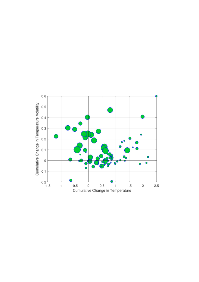
Figure 2: Correlation between temperature level and volatility

The rise in volatility was relatively larger in Europe, Central Asia and North America, which were only marginally affected by the increase in temperature levels. This divergence is interesting per se and it is also useful for identification: if levels and volatilities were highly correlated, it would be hard to disentangle their effects. To investigate this point further, in Figure 2 we show the relation between temperature levels and volatilities at the country level. The scatter plot relates the cumulative change in temperatures recorded between 1961 and 2005 (horizontal axis) to the cumulative change in temperature volatility estimated by the model (vertical axis). There is no correlation between changes in levels and volatilities. In Section 3.2 we rely on a more stringent identification strategy to estimate the impact of volatility shocks; the model allows us to control for country and/or time fixed effects as well as the lagged influence of GDP and temperatures. However, the lack of correlation in figure Figure 2 yields preliminary evidence that there is enough information in the data to separate level and volatility effects. The scatter plot also shows that the increase in volatility has been more widespread than the increase in average temperatures. In particular, many large economies experienced a rise in volatility combined with constant or decreasing average temperatures (see north-western quadrant).

Two further points are worth making. The change in volatilities over time is highly significant from a statistical perspective. Figure A5 of the annex shows the estimated average within-region volatility series together with a 68% (one standard deviation) posterior coverage band. The null hypothesis that volatility did not change between the 1960s and the early 2000s can be safely rejected in all regions. In all but two cases, i.e. Sub-Saharan Africa and Eastern Europe, volatility follows a clear upward trend at least since the 1980s. At the same time, regional aggregations mask a significant degree of heterogeneity at the country level. In figure A6 we compare the confidence bands calculated at the regional level to the central estimates of the country-specific volatilities. It is immediately clear that level, variability and medium-run patterns in temperature volatility differ widely across countries even within a given geographical region. The panel VAR allows us to exploit these forms of cross-country heterogeneity to identify the causal effects of an exogenous change in temperature volatility.

3.2 The impact of temperature volatility on growth

The panel VAR introduced in Section 2 captures a number of interactions involving both the level and the volatility of annual temperatures and GDP growth at the country level. The posterior mean and standard deviation of the parameters for the baseline model is summarized in table A1 of the annex. The estimates highlight a potentially important influence of volatility on both GDP and temperatures: all else equal, a rise in temperature volatility $h^{T}$ is associated with lower growth and higher temperatures. A rise in $h^{GDP}$ is also associated with lower growth rates, which is consistent with the negative effects of economic volatility on investment highlighted in the literature. Finally, $h^{T}$ and $h^{GDP}$ are both highly persistent, suggesting that the sample is characterized by slow transitions between calm and volatile phases rather than sudden and short-lived outbursts of volatility.

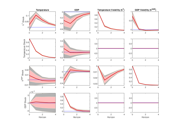
Figure 3: Impulse-response functions

In Figure 3 we report the impulse-response functions associated to the four shocks included in the model. For each variable the figure reports the estimated mean response with 90% and 68% posterior coverage bands. The first row of the figure shows the impact of an exogenous +1${}^{\text{o}}$C increase in temperature volatility ($h^{T}$, column 3). The shock causes an increase in temperatures, a decline in GDP growth and an increase in the volatility of the GDP process. The responses are statistically significant and fairly large in quantitative terms: GDP drops by 0.3 percent on impact and remains below equilibrium for four years (col. 2), while the conditional volatility of the GDP growth rate rises by about 0.75 percentage points (col. 4). The results imply that countries that experience high temperature volatility in a given year are likely to grow less and face more pronounced GDP fluctuations in the medium term. In other words, higher temperature volatility brings along a weaker and riskier growth path. It is worth emphasizing that the transmission mechanism hinges on temperature risk rather than actual changes in temperature levels. First, $h^{T}_{i,t}$ measures by construction the conditional volatility of temperatures in country $i$, and it is unrelated to the weather patterns observed in $i$ in the past. Second, the model controls for the influence of both contemporaneous and past temperature shocks on GDP growth. Third, the estimates remain unaltered if we include squared annual changes in temperatures or precipitations to control for the confounding influence of ‘extreme’ weather events (see Section 4). Hence, the results show that economic agents respond to the degree of expected variability of the environment, and that – as in the case of many other non-climatic factors – lower predictability is per se detrimental for growth.

Figure 3 shows that temperature and output shocks have negligible implications for the system, except for raising respectively $T_{t}$ and $\Delta GDP_{t}$ (rows 2 and 4). The impact of a temperature increase on GDP is positive but non-significant in the baseline specification, but it becomes negative if the model is estimated over poor countries only (see Section 4). Both results are in line with those reported in DJO. Interesting results emerge for shocks to the volatility of the GDP process ($h^{GDP}$, row 3). A rise in GDP volatility has a negative impact on the GDP growth rate, consistent with the well-known influence of macroeconomic uncertainty on economic activity (see e.g. Bloom (2014) and Fernández-Villaverde and Guerrón-Quintana (2020)). However, the impact is smaller and extremely short-lived: instead of a protracted slowdown, the shock causes a one-year drop followed by a quick rebound with mild signs of ‘overshooting’. This has important implications for the intepretation of the results in the first row of Figure 3. On the one hand, endogenous increases in macroeconomic volatility contribute to the propagation of temperature volatility shocks. One of the reasons why temperature volatility reduces economic activity is that it makes the growth rate of the economy less predictable. On the other hand, this volatility spillover must be part of a more complex transmission mechanism. The change in macroeconomic volatility per se does not account for the decline in GDP, particularly over longer horizons, suggesting that temperature volatility has an additional, direct effect on the economy. We investigate the nature of the transmission mechanism more closely in Section 5.

The analysis carried out in this Section leads to two conclusions. First, temperature volatility has risen steadily across countries since the 1960s, rendering climate conditions less predictable over time. Second, controlling for temperature levels, a rise in temperature volatility is followed by a period of low and volatile GDP growth rates. Taken together, these findings point to two distinct mechanisms through which climate change could affect income and welfare over and above the well-known ‘global warming’ phenomenon. In the next section we examine the robustness of the baseline results along various dimensions, considering inter alia the role of precipitations, cross-country heterogeneity, the relation between volatility and extreme events, and the alternative CRU-TS climate dataset.

4 Robustness and extensions

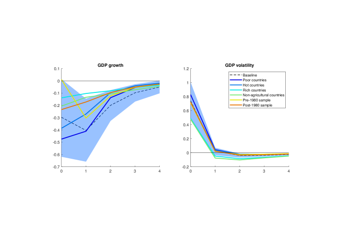
Figure 4: Heterogeneity

In this section we replicate the baseline analysis using alternative specifications and estimation samples for the panel VAR model. To save space we only discuss the impact of temperature volatility shocks on level and conditional volatility of the GDP growth rate; the online annex provides more details. The main results of the tests are summarized in figures 4 to 6 and in tables 1 and 2. The figures compare the impulse-response functions from the alternative specifications to those obtained in the baseline case. The tables report the central estimates of the short-run and long-run impacts of the shock on GDP in each model, along with the corresponding 68% posterior coverage intervals.

4.1 Heterogeneity

There is an open debate on the cross-sectional and distributional implications of climate change. In particular, rising temperatures may affect only or mostly poor countries that rely heavily on agricolture and have limited adaptation capabilities (see Section 1). The first issue we investigate is thus how the macroeconomic effects of climate volatility vary across regions. We re-estimate the baseline panel VAR specifications using only data on “poor”, “rich”, “hot”, or “non-agricultural” countries. All groups are defined using the dummy variables suggested by DJO. Poor is a dummy for countries that have below-median GDP per capita in their first year in the dataset, hot is dummy for countries with above-median average temperature in the 1950s, and agricultural is a dummy for countries with an above-median share of GDP in agriculture in 1995. The estimates are reported in Figure 4, which compares the impact on GDP of a one-standard deviation increase in temperature volatility obtained in the four alternative subsamples. The responses are qualitatively similar across samples: in all cases GDP growth is lower and more volatile on impact, i.e. in the year when volatility rises, and for up to four years after the shock. The differences across subsamples largely mirror those documented for temperature levels: rich and non-agricultural countries are less affected than poor or hot countries. However, heterogeneity is less pronounced. On impact, the shock raises GDP volatility in all groups of countries, but it causes a statistically significant GDP contraction only in poor and hot countries (see table 1). At the five-year horizon the situation is reversed: the cumulative GDP response becomes significant for all groups, while the volatility response is only significant for poor and hot countries (see table 2). This suggests that rich countries smooth the impact of the shock rather than averting it altogether. They insulate GDP from shocks that take place within a given year, and succeed in mitigating the macroeconomic uncertainty caused by those shock, but they cannot avoid the longer-term implications of higher temperature volatility. The estimates GDP loss caused by a +1${}^{\text{o}}$C increase in temperature volatility is -0.48% for rich countries and -1.14% for poor countries. All in all, the evidence indicates that climate volatility matters even for highly-developed economies that can adjust efficiently to gradual changes in temperature levels.

The last two lines in Figure 4 show the response obtained estimating the model separately on pre- or post-1980 observations. The GDP response is slower in the earlier sample, but the pattern of the impulse-response functions is otherwise fairly similar. Tables 1 and 2 confirm that, although the contemporaneous GDP response is not significant before 1980, the long-term response is significant and almost identical in the two samples (-0.5% versus -0.6%).

4.2 Alternative specifications

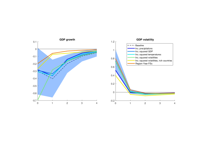
Figure 5: Additional controls

As a next step, we extend the baseline model to account for other factors that might affect the climate-growth nexus. The results of these tests are displayed in figure 5. We first replicate the baseline analysis adding to the model precipitations ($P_{it}$, in units of 100 mm per year), which are routinely employed together with temperatures as a proxy of climatic change. The identification of the shocks is again based on a recursive ordering of the variables. We place precipitations before GDP so to maintain the assumption that the climate is exogenous to macroeconomic shocks in the short term (see Section 2). This model delivers slightly smaller estimates of the peak impact of temperature volatility shocks on GDP and GDP volatility, but the responses remain statistically significant (see table 1).

A particularly critical issue is the potential nonlinearity of the link between climate and the economy. Output and productivity decline globally when temperatures move significantly below or above 13${}^{\text{o}}$C (Burke et al., 2015). Mortality rates rise sharply in the US in areas and periods in which temperatures reach the upper percentiles of their distribution (Deschênes and Greenstone, 2011; Barreca et al., 2016). Furthermore, weather anomalies are known to have a large negative impact on the economy (Dell et al., 2014; Kim et al., 2021). This creates a non-trivial identification challenge: from an empirical perspective, a volatility proxy could simply capture the nonlinear impact of large shocks to temperature levels. In previous studies on the relation between climate volatility and growth, Donadelli et al. (2020), Kotz et al. (2021) and Linsenmeier (2021) employed realized (ex-post) volatility or variability measures that are by construction affected by the occurrence of large fluctuations in weather conditions. Donadelli et al. (2020) report a correlation between temperature volatility and extreme events – defined as heavy rainfalls, floods, frosts, hot temperature anomalies and droughts – of 0.59 in the UK in the post-war period (see figure 1 of the paper). Kotz et al. (2021) obtain an annual variability measure by calculating the intra-monthly standard deviation of daily temperatures and then averaging it over 12 months. The averaging step ameliorates the problem but it is unlikely to solve it completely: we find that in the pooled dataset the indicator has a correlation of 0.30 with the squared change in annual temperatures In Linsenmeier (2021) day-to-day variability (which is heavily affected by large shocks) has indeed a stronger economic impact than seasonal or interannual variability (which are smoother and less affected by those shocks due to temporal aggregation). The upshot is that the relation between realized volatility and GDP may mask the impact of nonlinearities and large shocks rather than a genuine uncertainty component.

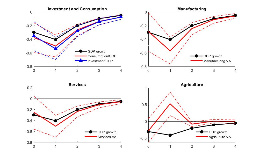
Figure 7: Transmission of temperature volatility shocks

Our ex-ante volatility measures are not subject to this limitation because they are not constructed using (and are thus unrelated to) past temperatures. However, the identification problem may in principle arise in our case as well. As a first check we examine the correlation between changes in the estimated conditional temperature volatilities ($h^{T}_{i,t}$) and squared annual changes in temperatures, precipitations and income ($T_{i,t}$, $P_{i,t}$, $GDP_{i,t}$). These provide rough estimates of the realized annual volatility of the three series, capturing a range of ’extreme events’ – i.e. large year-to-year shifts in temperatures, precipitations or GDP – that may potentially bias the estimation of the climate risk effect. The correlations are extremely low for all geographical regions, which means that fluctuations in $h^{T}_{i,t}$ do not systematically overlap with large year-on-year changes in output or weather conditions (see figure 7 in the annex). We then re-estimate the panel VAR adding to the baseline variables squared GDP growth rates, squared temperatures, or the squared volatility terms. As figure 5 shows, none of these changes has major implications for our results. The contemporaneous impact of the shock on GDP growth and GDP volatility is virtually unaffected by the inclusion of squared GDP and temperatures, and it almost doubles when squared volatilities are added to the model (see 1). Furthermore, the long-run impact of the shock on GDP varies between -0.9% and -1.3%, close to the baseline estimate of -1.1% (see table 2). The tables show that, in the case of rich countries, both the short-term and the long-term impact of the shock become in fact larger and more significant when the squared volatility terms are added to the model. These results corroborate the conclusion that the model picks up the specific influence of the conditional volatility of annual temperatures rather than nonlinearities involving past GDP and/or realized temperature fluctuations.

As a final test, we estimate the baseline model including a set of year$\times$region fixed effects to control for the potential influence of unobserved and time-varying drivers of GDP growth. The GDP volatility response is virtually unaffected by the change, while the GDP response becomes smaller and less persistent (see figure 5). The estimated short- and long-run GDP responses drop respectively to -0.2% and -0.3%. Both are statistically significant. This confirms that, although the baseline estimates may be somewhat distorted by specific subperiods or regional trends, temperature volatility has a specific well-defined influence on economic growth.

4.3 An alternative climate dataset

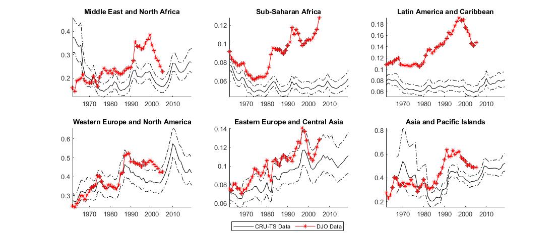
Figure 6: Temperature volatility in the CRU-TS dataset

The DJO dataset facilitates a comparison between our results and those available in the literature, but it ends in 2005. Below we replicate the estimation of the baseline model using the Climatic Research Unit gridded Time Series (CRU TS) dataset produced by the UK’s National Centre for Atmospheric Science, that covers a longer sample ending in 2019. The data is described in detail in Harris et al. (2020). CRU-TS relies on more recent techniques to interpolate station-level weather observations; it also employs area-weighted rather than population-weighted averages to construct country-level observations, allowing us to examine the robustness of our conclusions along another important dimension. Figure 6 compares the temperature volatility series obtained by estimating the baseline panel VAR model on the two datasets. The estimates follow fairly similar patterns over the 1960-2005 period in four of the six regions. Temperature volatility rose markedly in Europe, North America and Asia (bottom row) and remained roughly constant in the Middle East and North Africa (top left panel). The magnitude of the rise in volatility is also generally similar; for Western Europe and North America, for instance, volatility is estimated to rise from about 0.2${}^{\text{o}}$C in 1965 to 0.4${}^{\text{o}}$C in 2005. Larger differences appear in the case of Sub-Saharan Africa and Latin America, for which volatilities rise in the DJO data and remain constant in the CRU-TS data. The presence of large and sparsely populated countries makes the weighting scheme more influential in these regions. The CRU-TS data also shows that volatility rose or remained constant from 2005 onwards. Tables 1 and 2 show that temperature volatility shocks have similar implications in the two datasets. The estimated impact of the shocks is actually larger and statistically more significant in the CRU-TS dataset: a +1${}^{\text{o}}$C increase in volatility causes GDP to drop by 0.4% on impact and 1.3% in the long run. The conditional volatility of GDP also rises more compared to the baseline.

5 Transmission mechanisms

Pinning down the mechanisms through which climate shocks affect the economy is difficult because these shocks influence a broad range of outcomes, including inter alia output, productivity, health or migrations (Dell et al., 2014). Climate conditions affect aggregate supply directly, through their impact on infrastructures, natural resources and trade flows; but they can also shift aggregate demand by influencing households’ income, wealth and consumption patterns (Batten et al., 2020). The transmission mechanisms are also likely to vary across countries. Natural disasters have a null or mildly negative impact on inflation in rich countries, but cause long-lasting price increases in emerging countries (Parker, 2018). Among OECD countries, spikes in green-house gas emissions trigger joint declines in output and prices that mimic a weakening in aggregate demand (Ciccarelli and Marotta, 2021). In short, there seems to be no single dominant transmission mechanism for the ‘level’ shocks traditionally studied in the climate literature. Our simulations based on the Basu and Bundick (2017) model suggest that the propagation of volatility shocks is equally complex: a rise in volatility causes a slowdown under a broad range of model configurations, but the relative movements in consumption, investment and prices vary depending on the mechanism that links temperatures to the fundamentals of the economy (see section A of the online annex).

To shed light on the transmission mechanisms we estimate an additional set of panel VAR specifications in which GDP growth is replaced by alternative, more disaggregated indicators of economic activity. We first consider investment (defined as gross capital formation) and total consumption expenditure, both expressed as percentages of GDP. The top left panel of Figure 7 shows the responses of these variables to the 1${}^{\text{o}}$C increase in temperature volatility examined in the previous section. The GDP response obtained from the baseline model is also shown for comparison. Investment and consumption drop by a maximum of about 0.5 percentage points, following a trajectory that closely follows that of GDP. We next examine the annual growth rate of value added (VA) in the manufacturing, services and agricultural sector. VA captures changes in productivity and in the price and/or mix of production factors employed in each sector. A rise in volatility has a persistent negative impact on manufactures and services, consistent with a generalized drop in productivity or a less intense utilization of capital. The shock has instead a positive but short-lived impact on agriculture; one possibility is that VA is driven in this case by a relatively large increase in the price of the final goods (see Loayza et al., 2012). The estimates in figure 7 paint a fairly clear picture. An exogenous rise in temperature volatility causes a drop in consumption and fixed investment that is consistent with the precautionary response and the wait-and-see effect that are generally associated to a rise in economic or financial uncertainty. Furthermore, volatility shocks, like changes in realized temperatures, cause a slowdown that spreads widely across the main sectors of the economy. We leave a more granular, geographically-differentiated investigation of the transmission mechanisms to future work.

6 Conclusions

Rising temperatures are known to have a negative impact on economic growth, particularly in poor countries. This paper shows that climate change also affects economic outcomes through a volatility channel. We use a panel VAR model with stochastic volatility to identify exogenous changes in temperature volatility and assess their implications for the macroeconomy. We exploit the model to estimate the conditional volatility of annual temperatures for 133 countries between 1961 and 2019. These estimates capture the variability of the residual component of annual temperatures that cannot be predicted using past data, quantifying the ex-ante ‘temperature risk’ faced by households and firms in a given country at a given point in time. The model captures the interaction between levels and variances of annual temperatures and GDP growth rates, allowing the identification of exogenous temperature volatility shocks. The analysis yields two main conclusions. First, temperature volatility increased steadily over time, even in regions that were only marginally affected by global warming. Second, temperature volatility matters for growth. Changes in volatility affect both the means and the variances of the GDP growth rates of the countries in our sample. Controlling for temperature levels, a +1${}^{\text{o}}$C increase in volatility causes on average a 0.3 per cent decline in GDP growth and a 0.7 per cent increase in the volatility of the GDP growth rate. These mechanisms operate in rich, non-agricultural countries too, and they are statistically and economically significant even controlling for the influence of large realized fluctuations in GDP, temperatures or precipitations. Our findings demonstrate that economic agents respond to changes in the expected variability of the environment. They also suggests that climate risk may have important ex-ante implications for welfare, as uncertainty has economic costs that can materialize before, and independently of, any observed change in temperatures.

	GDP				GDP volatility
	16%	50%	84%		16%	50%	84%
Baseline	-0.492	-0.297	-0.102		0.597	0.741	0.896
Poor countries	-0.772	-0.475	-0.162		0.624	0.828	1.024
Hot countries	-0.663	-0.386	-0.121		0.543	0.720	0.903
Rich countries	-0.308	-0.138	0.028		0.314	0.488	0.650
Non-agricultural countries	-0.416	-0.206	0.006		0.278	0.478	0.681
Pre-1980 sample	-0.312	0.011	0.339		0.593	0.710	0.829
Post-1980 sample	-0.426	-0.234	-0.043		0.604	0.723	0.844
Inc. precipitations	-0.443	-0.282	-0.116		0.393	0.520	0.655
Inc. squared GDP	-0.482	-0.290	-0.098		0.584	0.732	0.874
Inc. squared temperatures	-0.501	-0.310	-0.115		0.575	0.724	0.872
Inc. squared volatilities	-0.957	-0.693	-0.444		0.567	0.723	0.873
Inc. squared volatilities, rich cts	-0.492	-0.269	-0.059		0.224	0.393	0.561
Region-Year FEs	-0.355	-0.198	-0.030		0.670	0.794	0.917
CRU-TS dataset	-0.575	-0.394	-0.210		0.946	1.118	1.286

Table 1: Short-term impact of an increase in temperature volatility.
Contemporaneous responses of GDP levels and GDP volatilities to an exogenous 1${}^{\text{o}}$C increase in the conditional volatility of annual temperatures ($h^{T}_{i,t}$). The responses are measured in the year when the shock takes place. The rows refer to alternative specifications of the panel VAR model: for each specification, the table reports the median responses along with the 16th and 84th percentiles of the posterior distribution. The sample includes 133 countries and it covers the 1961-2005 period, except for the CRU-TS dataset that runs to 2019.

	GDP				GDP volatility
	16%	50%	84%		16%	50%	84%
Baseline	-1.486	-1.103	-0.746		0.419	0.616	0.822
Poor countries	-1.618	-1.144	-0.643		0.516	0.776	1.019
Hot countries	-1.292	-0.855	-0.413		0.442	0.669	0.896
Rich countries	-0.874	-0.483	-0.075		-0.108	0.153	0.394
Non-agricultural countries	-1.132	-0.639	-0.143		-0.195	0.091	0.383
Pre-1980 sample	-0.952	-0.519	-0.086		0.497	0.647	0.793
Post-1980 sample	-1.031	-0.600	-0.179		0.469	0.630	0.787
Inc. precipitations	-0.237	-0.105	0.028		1.237	1.283	1.335
Inc. squared GDP	-1.327	-0.964	-0.591		0.402	0.600	0.795
Inc. squared temperatures	-1.326	-0.961	-0.581		0.384	0.590	0.781
Inc. squared volatilities	-1.750	-1.351	-0.931		0.338	0.547	0.744
Inc. squared volatilities, rich cts	-0.984	-0.504	-0.048		-0.206	0.046	0.301
Region-Year FEs	-0.627	-0.323	-0.015		0.562	0.731	0.892
CRU-TS dataset	-1.687	-1.320	-0.934		0.945	1.157	1.358

Table 2: Long-term impact of an increase in temperature volatility.
Long-run response of GDP levels and GDP volatilities to an exogenous 1${}^{\text{o}}$C increase in the conditional volatility of annual temperatures ($h^{T}_{i,t}$). The responses are measured 5 years after the materialization of the shock; the GDP response is calculated cumulating changes in growth rates over the 5-year horizon. The rows refer to alternative specification of the panel VAR model: for each specification, the table reports the median responses along with the 16th and 84th percentiles of the posterior distribution. The sample includes 133 countries and it covers the 1961-2005 period, except for the CRU-TS dataset that runs to 2019.

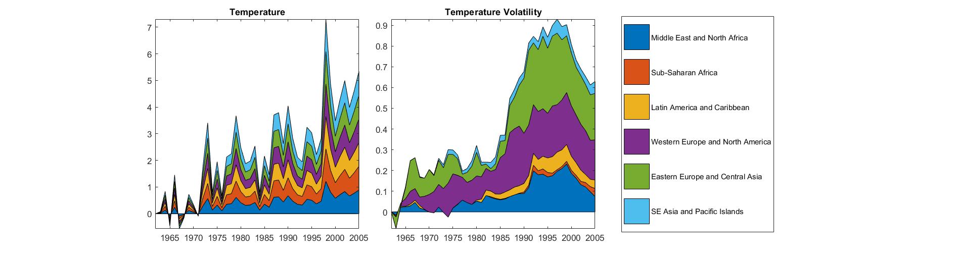
Figure 1: Trends in temperatures and temperature volatility

The left panel shows the cumulative change in annual temperatures recorded between 1961 and 2005 in each of the six geographical regions listed in the legend. The right panel shows the cumulative change in each region’s temperature volatility estimated by the panel VAR model. All figures are in degrees Celsius. The sample includes 133 countries and the regions are summarized by simple (unweighted) averages of country-level estimates.

Total change in annual temperatures (horizontal axis) versus total change in estimated temperature volatilities (vertical axis). Temperatures and volatilities are in degrees Celsius. The sample includes 133 countries between 1961 and 2005. The size of the bubbles represents the countries’ average GDP levels in the 1950-1959 period.

Responses to level and volatility shocks in the baseline model. The estimates are obtained from a country-level panel VAR model where volatility is stochastic and changes in volatility influence the dynamics of all endogenous variables. Temperature and GDP are average annual temperature and annual GDP growth rate; $h^{T(GDP)}$ denotes the estimated conditional volatility of the temperature (GDP) series. The figure shows the responses to a 1${}^{\text{o}}$C increase in $h^{T}$ (row 1), a 1${}^{\text{o}}$C increase $Temperature$, a 1 percentage point increase in $h^{GDP}$ (row 3) and a 1 percentage point increase in $GDP$ (row 4). In all cases we report the mean responses with 68% and 90% posterior coverage bands. The estimation sample includes 133 countries between 1961 and 2005.

Impact of a 1${}^{\text{o}}$C increase in temperature volatility on the annual growth rate of GDP (left panel) and its conditional volatility (right panel). The shaded area is the 90% posterior coverage band obtained from the baseline specification of the panel VAR model. The additional lines represent the central estimates obtained restricting the estimation to a subsample of poor, hot, rich or non-agricoltural countries, or splitting the sample in 1980.

Impact of a 1${}^{\text{o}}$C increase in temperature volatility on the annual growth rate of GDP (left panel) and its conditional volatility (right panel). The shaded area is the 90% posterior coverage band obtained from the baseline specification of the panel VAR model. The additional lines represent the central estimates obtained by alternatively including in the model average yearly precipitations, squared GDP growth rates, squared temperatures, squared GDP and temperature volatilities, or a set of region-by-year fixed effects.

The figure compares the conditional volatility of annual temperatures in the Climatic Research Unit gridded Time Series dataset (CRU-TS, in black) to those in the Dell et al. (2012) dataset (DJO, in red). For the CRU-TS data we report the 16th and 84th percentiles of the posterior distribution along with the median estimates. All series are obtained using the baseline specification of the panel VAR model and are expressed in Celsius degrees. See notes to figure 1.

The figure shows the impact of a 1${}^{\text{o}}$C increase in temperature volatility on the consumption-to-GDP and investment-to-GDP ratios (top left panel) and on the annual growth rates of value added in the manufacturing, services and agricultural sectors (top right and bottom panels). All panels include for comparison the estimated impact of the shock on annual GDP growth derived from the baseline panel VAR model. The estimation sample includes 133 countries between 1961 and 2005.

References

- Acemoglu et al. (2012) Acemoglu, D., P. Aghion, L. Bursztyn, and D. Hemous (2012, February). The environment and directed technical change. American Economic Review 102(1), 131–66.
- Andrieu et al. (2010) Andrieu, C., A. Doucet, and R. Holenstein (2010). Particle markov chain monte carlo methods. Journal of the Royal Statistical Society: Series B (Statistical Methodology) 72(3), 269–342.
- Arias et al. (2021) Arias, P., N. Bellouin, E. Coppola, R. Jones, G. Krinner, J. Marotzke, V. Naik, M. Palmer, G.-K. Plattner, J. Rogelj, et al. (2021). Climate change 2021: The physical science basis. contribution of working group14 i to the sixth assessment report of the intergovernmental panel on climate change.
- Bansal et al. (2016) Bansal, R., D. Kiku, and M. Ochoa (2016). Price of long-run temperature shifts in capital markets. Technical report, National Bureau of Economic Research.
- Bansal et al. (2014) Bansal, R., D. Kiku, I. Shaliastovich, and A. Yaron (2014). Volatility, the macroeconomy, and asset prices. The Journal of Finance 69(6), 2471–2511.
- Barreca et al. (2016) Barreca, A., K. Clay, O. Deschenes, M. Greenstone, and J. S. Shapiro (2016). Adapting to climate change: The remarkable decline in the us temperature-mortality relationship over the twentieth century. Journal of Political Economy 124(1), 105–159.
- Basu and Bundick (2017) Basu, S. and B. Bundick (2017). Uncertainty shocks in a model of effective demand. Econometrica 85(3), 937–958.
- Batten et al. (2020) Batten, S., R. Sowerbutts, and M. Tanaka (2020). Climate change: Macroeconomic impact and implications for monetary policy. Ecological, Societal, and Technological Risks and the Financial Sector, 13–38.
- Bloom (2009) Bloom, N. (2009). The impact of uncertainty shocks. Econometrica 77(3), 623–685.
- Bloom (2014) Bloom, N. (2014). Fluctuations in uncertainty. The Journal of Economic Perspectives 28(2).
- Bolton and Kacperczyk (2020) Bolton, P. and M. Kacperczyk (2020). Do investors care about carbon risk? Technical report, National Bureau of Economic Research.
- Burke and Emerick (2016) Burke, M. and K. Emerick (2016, August). Adaptation to climate change: Evidence from us agriculture. American Economic Journal: Economic Policy 8(3), 106–40.
- Burke et al. (2015) Burke, M., S. M. Hsiang, and E. Miguel (2015). Global non-linear effect of temperature on economic production. Nature 527(7577), 235–239.
- Burke and Leigh (2010) Burke, P. J. and A. Leigh (2010, October). Do output contractions trigger democratic change? American Economic Journal: Macroeconomics 2(4), 124–57.
- Calel et al. (2020) Calel, R., S. C. Chapman, D. A. Stainforth, and N. W. Watkins (2020). Temperature variability implies greater economic damages from climate change. Nature communications 11(1), 1–5.
- Choi et al. (2020) Choi, D., Z. Gao, and W. Jiang (2020, 02). Attention to Global Warming. The Review of Financial Studies 33(3), 1112–1145.
- Christiano et al. (2014) Christiano, L. J., R. Motto, and M. Rostagno (2014, January). Risk shocks. American Economic Review 104(1), 27–65.
- Ciccarelli and Marotta (2021) Ciccarelli, M. and F. Marotta (2021). Demand or supply? an empirical exploration of the effects of climate change on the macroeconomy. ECB Working Paper 2608.
- Clark (2011) Clark, T. E. (2011). Real-time density forecasts from bayesian vector autoregressions with stochastic volatility. Journal of Business & Economic Statistics 29(3), 327–341.
- Cogley and Sargent (2005) Cogley, T. and T. J. Sargent (2005). Drifts and volatilities: monetary policies and outcomes in the post wwii us. Review of Economic dynamics 8(2), 262–302.
- Dell et al. (2009) Dell, M., B. F. Jones, and B. A. Olken (2009). Temperature and income: reconciling new cross-sectional and panel estimates. American Economic Review 99(2), 198–204.
- Dell et al. (2012) Dell, M., B. F. Jones, and B. A. Olken (2012, July). Temperature shocks and economic growth: Evidence from the last half century. American Economic Journal: Macroeconomics 4(3), 66–95.
- Dell et al. (2014) Dell, M., B. F. Jones, and B. A. Olken (2014). What do we learn from the weather? the new climate-economy literature. Journal of Economic Literature 52(3), 740–98.
- Deschênes and Greenstone (2007) Deschênes, O. and M. Greenstone (2007). The economic impacts of climate change: evidence from agricultural output and random fluctuations in weather. American Economic Review 97(1), 354–385.
- Deschênes and Greenstone (2011) Deschênes, O. and M. Greenstone (2011). Climate change, mortality, and adaptation: Evidence from annual fluctuations in weather in the us. American Economic Journal: Applied Economics 3(4), 152–85.
- Donadelli et al. (2020) Donadelli, M., M. Jüppner, A. Paradiso, and C. Schlag (2020). Computing macro-effects and welfare costs of temperature volatility: A structural approach. Computational Economics, 1–48.
- Fernández-Villaverde and Guerrón-Quintana (2020) Fernández-Villaverde, J. and P. A. Guerrón-Quintana (2020). Uncertainty shocks and business cycle research. Review of economic dynamics 37, S118–S146.
- Fisher et al. (2012) Fisher, A. C., W. M. Hanemann, M. J. Roberts, and W. Schlenker (2012). The economic impacts of climate change: evidence from agricultural output and random fluctuations in weather: comment. American Economic Review 102(7), 3749–60.
- Giglio et al. (2020) Giglio, S., B. T. Kelly, and J. Stroebel (2020). Climate finance. Technical report, National Bureau of Economic Research.
- Golosov et al. (2014) Golosov, M., J. Hassler, P. Krusell, and A. Tsyvinski (2014). Optimal taxes on fossil fuel in general equilibrium. Econometrica 82(1), 41–88.
- Harris et al. (2020) Harris, I., T. J. Osborn, P. Jones, and D. Lister (2020). Version 4 of the cru ts monthly high-resolution gridded multivariate climate dataset. Scientific data 7(1), 1–18.
- Hassler et al. (2016) Hassler, J., P. Krusell, and A. A. Smith Jr (2016). Environmental macroeconomics. In Handbook of macroeconomics, Volume 2, pp. 1893–2008. Elsevier.
- Hong et al. (2020) Hong, H., G. A. Karolyi, and J. A. Scheinkman (2020). Climate finance. The Review of Financial Studies 33(3), 1011–1023.
- Jurado et al. (2015) Jurado, K., S. C. Ludvigson, and S. Ng (2015, March). Measuring uncertainty. American Economic Review 105(3), 1177–1216.
- Kahn et al. (2021) Kahn, M. E., K. Mohaddes, R. N. Ng, M. H. Pesaran, M. Raissi, and J.-C. Yang (2021). Long-term macroeconomic effects of climate change: A cross-country analysis. Energy Economics, 105624.
- Kim et al. (2021) Kim, H. S., C. Matthes, and T. Phan (2021). Extreme weather and the macroeconomy. Available at SSRN 3918533.
- Kotz et al. (2021) Kotz, M., L. Wenz, A. Stechemesser, M. Kalkuhl, and A. Levermann (2021). Day-to-day temperature variability reduces economic growth. Nature Climate Change 11(4), 319–325.
- Krueger et al. (2020) Krueger, P., Z. Sautner, and L. T. Starks (2020). The importance of climate risks for institutional investors. The Review of Financial Studies 33(3), 1067–1111.
- Li et al. (2020) Li, Q., H. Shan, Y. Tang, and V. Yao (2020). Corporate climate risk: Measurements and responses.
- Lindsten et al. (2015) Lindsten, F., P. Bunch, S. S. Singh, and T. B. Schön (2015, May). Particle ancestor sampling for near-degenerate or intractable state transition models. arXiv e-prints, arXiv:1505.06356.
- Lindsten et al. (2014) Lindsten, F., M. I. Jordan, and T. B. Schön (2014). Particle gibbs with ancestor sampling. Journal of Machine Learning Research 15, 2145–2184.
- Linsenmeier (2021) Linsenmeier, M. (2021). Temperature variability and long-run economic development.
- Loayza et al. (2012) Loayza, N. V., E. Olaberria, J. Rigolini, and L. Christiaensen (2012). Natural disasters and growth: Going beyond the averages. World Development 40(7), 1317–1336.
- Nordhaus and Moffat (2017) Nordhaus, W. D. and A. Moffat (2017). A survey of global impacts of climate change: replication, survey methods, and a statistical analysis.
- Parker (2018) Parker, M. (2018). The impact of disasters on inflation. Economics of Disasters and Climate Change 2(1), 21–48.
- Sautner et al. (2020) Sautner, Z., L. van Lent, G. Vilkov, and R. Zhang (2020). Firm-level climate change exposure. manuscript.
- Stern (2016) Stern, N. (2016). Economics: Current climate models are grossly misleading. Nature News 530(7591), 407.
- Tol (2009) Tol, R. S. (2009). The economic effects of climate change. Journal of economic perspectives 23(2), 29–51.