Lossless Convexification and Duality

Abstract

The main goal of this paper is to investigate strong duality of non-convex semidefinite programming problems (SDPs). In the optimization community, it is well-known that a convex optimization problem satisfies strong duality if the Slater’s condition holds. However, this result cannot be directly generalized to non-convex problems. In this paper, we prove that a class of non-convex SDPs with special structures satisfies strong duality under the Slater’s condition. Such a class of SDPs arises in SDP-based control analysis and design approaches. Throughout the paper, several examples are given to support the proposed results. We expect that the proposed analysis can potentially deepen our understanding of non-convex SDPs arising in the control community, and promote their analysis based on KKT conditions.

,

1 Introduction

Advances of convex optimization [1] and semidefinite programming (SDP) [2] techniques have made significant progresses in computational control analysis and design approaches [3, 4, 5, 6]. In the control community, it is well-known that many important control design problems, such as the state-feedback control design for linear time-invariant (LTI) systems, can be formulated as convex SDP or linear matrix inequality (LMI) problems, which can be efficiently solved using convex optimization tools. On the other hand, some classes of control problems cannot be expressed in terms of convex SDPs or LMIs. One of the representative problems is the static output-feedback problem, which is known to be NP-hard [7, 8, 9].

It is well-known that most convex SDP formulations of control problems are originally formulated as non-convex SDPs, but can be converted to convex SDPs through change of variables [10]. A natural question that arises here is if a non-convex SDP is equivalently transferable to a convex SDP via a change of variables, then can we potentially treat it as a convex SDP? More specifically, does the original non-convex SDP preserve some favorable properties of convex SDPs such as strong duality [1]?

In this paper, we answer this central question, and prove that a class of non-convex SDPs, which can be transferred to convex SDPs via changes of variables without introducing conservativeness, satisfies strong duality. To this end, we introduce a new concept called the lossless convexification, and prove that if there exists a lossless convexification of the original non-convex SDP, then it satisfies strong duality. Moreover, we provide examples of the state-feedback stabilization problem for LTI systems, which is one of the represented control problems that can be converted to LMIs via change of variables. It turns out that such a transformation that arises in the control community is an example of the lossless convexification, and the corresponding optimization problem satisfies strong duality. Finally, we expect that the proposed analysis can potentially deepen our understanding on non-convex SDPs arising in the control community, provide additional insights, and open new opportunities in analysis of non-convex SDPs based on Karush–Kuhn–Tucker (KKT) optimality conditions [11].

Related works: Duality has long been a core concept in optimal control theory such as the Pontryagin’s maximal principle. On the other hand, emergence of convex optimization [1] and SDP techniques in control analysis and design promoted new optimization formulations of control problems during the last decades. Accordingly, the corresponding duality has been studied to further deepen our understanding of classical control theories, e.g., [3, 12, 13, 14]. For instance, a new proof of Lyapunov’s matrix inequality was presented in [15] based on the standard SDP duality [2]. In addition, SDP formulations of the LQR problem and their dual formulations were developed in [13] and [14]. Comprehensive studies on the SDP dualities in systems and control theory, such as the Kalman-Yakubovich-Popov (KYP) lemma, the LQR problem, and the $H_{\infty}$-norm computation, were provided in [16]. A new Lagrangian duality result and its relation to reinforcement learning problems were established in [17] for infinite-horizon LQR problems. More recent results include the state-feedback solution to the LQR problem [18], the generalized KYP lemma and $H_{\infty}$ analysis [19, 20] derived using the Lagrangian duality. The recent paper, [18], proposed a new SDP formulation, where the finite-horizon LQR problem was converted into the optimal covariance matrix selection problem, and it can be also interpreted as a dual problem of the standard LQR approaches based on the Riccati equations or the Lyapunov methods. Compared to the existing works which address specific problems in the control community, the proposed result investigates general tools to identify strong duality of general non-convex SDPs.

Notation: The adopted notation is as follows: ${\mathbb{R}}$: set of real numbers  ${\mathbb{R}}^{n}$: $n$-dimensional Euclidean space; ${\mathbb{R}}^{n\times m}$: set of all $n\times m$ real matrices; $A^{T}$: transpose of matrix $A$; $A\succ 0$ ($A\prec 0$, $A\succeq 0$, and $A\preceq 0$, respectively): symmetric positive definite (negative definite, positive semi-definite, and negative semi-definite, respectively) matrix $A$; $A\succ B$ ($A\prec B$, $A\succeq B$, and $A\preceq B$, respectively): $A-B$ is symmetric positive definite (negative definite, positive semi-definite, and negative semi-definite, respectively); $I$: identity matrix with appropriate dimensions; ${\mathbb{S}}^{n}$: symmetric $n\times n$ matrices; ${\mathbb{S}}^{n}_{+}$: cone of symmetric $n\times n$ positive semi-definite matrices; ${\mathbb{S}}^{n}_{++}$: symmetric $n\times n$ positive definite matrices; $Tr(\cdot)$: trace of matrix $(\cdot)$; $\rho(A)$: spectral radius of a square matrix $A$, where the spectral radius stands for the maximum of the absolute values of its eigenvalues; $*$ inside a matrix: transpose of its symmetric term; s.t.: subject to; ${\bf relint}({\mathcal{D}})$: relative interior of a set ${\mathcal{D}}$; ${\bf dom}(f)$: domain of a function $f$.

2 Problem Formulation and Preliminaries

In this section, we briefly summarize basic concepts of the standard Lagrangian duality theory in [1]. Let us consider the following optimization problem with matrix inequalities (semidefinite programming, SDP), which is our main concern in this paper.

Problem 1 (Primal problem).

Solve for $x\in{\mathbb{R}}^{n}$

$$p^{*}:= \min_{x\in{\mathbb{R}}^{n}}f(x)\quad{\rm{s.t.}}\quad\Phi_{i}(x)\preceq 0,\quad i\in\{1,2,\ldots,N\}$$

where $x\in{\mathbb{R}}^{n}$, $\Phi_{i}:{\mathbb{R}}^{n}\to{\mathbb{S}}^{\hat{n}}$ is a continuous matrix function for all $i\in\{1,2,\ldots,N\}$, ${\hat{n}}$ is a positive integer, and $f:{\mathbb{R}}^{n}\to{\mathbb{R}}$ is a continuous objective function.

Note that in 1, we assume that the minimum point exists. Moreover, we assume that the domain, denoted by ${\mathcal{D}}:={\bf{dom}}\,(f)$, is nonempty. An important property of 1 that arises frequently is convexity.

Definition 1 (Convexity).

1 is said to be convex if $f$ is a convex function, and the feasible set, ${\mathcal{F}}:=\{x\in{\mathbb{R}}^{n}:\Phi_{i}(x)\preceq 0,i\in\{1,2,\ldots,N\}\}$, is convex.

Note that for the feasible set, ${\mathcal{F}}:=\{x\in{\mathbb{R}}^{n}:\Phi_{i}(x)\preceq 0,i\in\{1,2,\ldots,N\}\}$, to be convex, $\Phi_{i}(x)$ needs to be linear or convex in $x$ for all $i\in\{1,2,\ldots,N\}$ [1]. Another essential concept is the relative interior [1, pp. 23] defined below.

Definition 2 (Relative interior).

The relative interior of the set $\mathcal{D}$ is defined as

$${\bf{relint}}({\mathcal{D}}):=\{x\in{\mathcal{D}}:B(x,r)\cap{\bf{aff}}({\mathcal{D}})\subseteq{\mathcal{D}}\,\,{\rm{for}}\,\,{\rm{some}}\,\,r>0\},$$

where $B(x,r)$ is a ball with radius $r>0$ centered at $x$, and ${\bf{aff}}({\mathcal{D}})$ is the affine hull of ${\mathcal{D}}$ defined as the set of all affine combinations of points in the set $\mathcal{D}$ [1, pp. 23].

Associated with 1, the Lagrangian function [1] is defined as

$$L(x,\bar{\Lambda}):=f(x)+\sum\limits_{i=1}^{N}{Tr(\Lambda_{i}\Phi_{i}(x))}$$

for any $\Lambda_{i}\in{\mathbb{S}}^{\hat{n}}_{+},i\in\{1,2,\ldots,N\}$, called the Lagrangian multiplier, where $\bar{\Lambda}:=(\Lambda_{1},\Lambda_{2},\ldots,\Lambda_{N})$. For any $\Lambda_{i}\in{\mathbb{S}}^{\hat{n}}_{+},i\in\{1,2,\ldots,N\}$, we define the dual function as

$$g(\bar{\Lambda}):=\mathop{\inf}\limits_{x\in{\mathbb{R}}^{n}}L(x,\bar{\Lambda})=\mathop{\inf}\limits_{x\in{\mathbb{R}}^{n}}\left({f(x)+\sum\limits_{i=1}^{N}{Tr(\Lambda_{i}\Phi_{i}(x))}}\right).$$

It is known that the dual function yields lower bounds on the optimal value $p^{*}$:

$$g(\bar{\Lambda})\leq p^{*}$$ (1)

for any Lagrange multiplier, $\Lambda_{i}\in{\mathbb{S}}^{\hat{n}}_{+},i\in\{1,2,\ldots,N\}$. The Lagrange dual problem associated with 1 is defined as follows.

Problem 2 (Dual problem).

Solve for $\Lambda_{i}\in{\mathbb{S}}^{\hat{n}}_{+},i\in\{1,2,\ldots,N\}$

$$d^{*}:=\sup_{\Lambda_{i}\in{\mathbb{S}}^{\hat{n}}_{+},i\in\{1,2,\ldots,N\}}g(\bar{\Lambda}).$$

The dual problem is known to be concave even if the primal is not. In this context, the original 1 is sometimes called the primal problem. Similarly, $d^{*}$ is called the dual optimal value, while $p^{*}$ is called the primal optimal value. The inequality (1) implies the important inequality

$$d^{*}\leq p^{*},$$

which holds even if the original problem is not convex. This property is called weak duality, and the difference, $p^{*}-d^{*}$ is called the optimal duality gap. If the equality $d^{*}=p^{*}$ holds, i.e., the optimal duality gap is zero, then we say that strong duality holds.

Definition 3 (Strong duality).

If the equality, $d^{*}=p^{*}$, holds, then we say that strong duality holds for 1.

There are many results that establish conditions on the problem under which strong duality holds. These conditions are called constraint qualifications. Once such constraint qualification is Slater’s condition, which is stated below.

Lemma 1 (Slater’s condition).

Suppose that 1 is convex. If there exists an $x\in{\bf relint}({\mathcal{D}})$ such that

$$\Phi_{i}(x)\prec 0,\quad i\in\{1,2,\ldots,N\}$$

then strong duality holds, where ${\bf relint}({\mathcal{D}})$ is the relative interior [1, pp. 23] defined in Definition 2.

Without the constraint qualifications, such as the Slater’s condition, strong duality does not hold in general. A natural question is, under which conditions the strong duality holds for non-convex problems? Based on the ideas of Slater’s condition, we will explore a class of non-convex problems which satisfies strong duality throughout the paper. For more comprehensive discussions on the duality, the reader is referred to the monograph [1].

Assumption 1.

Slater’s condition holds for 1.

3 Main results

3.1 Lossless convexification

In this subsection, we will study convexification of matrix inequality constrained optimizations, which have a special property to be addressed soon. Toward this goal, let us consider the following optimization problem.

Problem 3.

Solve

$$\inf_{v\in h({\mathcal{D}})}f^{\prime}(v)\quad{\rm{s.t.}}\quad\Phi_{i}^{\prime}(v)\preceq 0,\quad i\in\{1,2,\ldots,N\}$$

for some mapping $h$ such that $h({\mathcal{D}})$ is convex, where $\Phi_{i}^{\prime}:{\mathbb{R}}^{n}\to{\mathbb{S}}^{\hat{n}},i\in\{1,2,\ldots,N\}$ and $f^{\prime}:{\mathbb{R}}^{n}\to{\mathbb{R}}$ are convex, and $f$ and $\Phi$ can be expressed as

$$f(x)= f^{\prime}(h(x))=(f^{\prime}\circ h)(x)$$

$$\Phi_{i}(x)= \Phi_{i}^{\prime}(h(x))=(\Phi_{i}^{\prime}\circ h)(x),\quad i\in\{1,2,\ldots,N\}.$$

Note that 3 is convex, and hence will be called a convexification of 1. In particular, we will consider a special convexification called the lossless convexification defined below.

Definition 4 (Lossless convexification).

Consider the following feasible sets associated with 1 and 3:

$${\mathcal{F}}:= \{x\in{\mathcal{D}}:,\Phi_{i}(x)\preceq 0,i\in\{1,2,\ldots,N\}\},$$ (2)

$${\mathcal{F}}^{\prime}:= \left\{{v\in h({\mathcal{D}}):\Phi_{i}^{\prime}(v)\preceq 0,i\in\{1,2,\ldots,N\}}\right\},$$ (3)

respectively, and suppose that the mapping $h$ whose domain restricted to $\mathcal{F}$ and codomain restricted to ${\mathcal{F}}^{\prime}$, i.e., $h:{\mathcal{F}}\to{\mathcal{F}}^{\prime}$, is a surjection. Then, 3 is said to be a lossless convexification of 1.

Note that $\mathcal{F}$ may be non-convex, while ${\mathcal{F}}^{\prime}$ is convex. In the sequel, simple examples are given to clearly illustrate the main notions of the lossless convexification.

Example 1.

Let us consider the optimization

$$\min_{x\in{\mathbb{R}}}\quad f(x)=x^{2}$$ (4)

$${\rm{s}}{\rm{.t}}.\quad\Phi_{1}(x)=-x^{2}+1\leq 0,$$

where $x\in{\mathbb{R}}$ is a decision variable. The corresponding constrained optimal solution is $x^{*}=1$, the primal optimal value is $p^{*}=1$, and ${\mathcal{D}}={\mathbb{R}}$. The feasible set is

$${\mathcal{F}}= \{x\in{\mathbb{R}}:-x^{2}+1\leq 0\}$$

$$= \{x\in{\mathbb{R}}:x\leq-1\}\cup\{x\in{\mathbb{R}}:x\geq 1\},$$

which is non-convex as depicted in Figure 1. Therefore, the optimization in (4) is non-convex. Now, let us consider the mapping

$$x\mapsto h(x)=-x^{2},$$

and the corresponding change of variable

$$v=h(x)=-x^{2}.$$

Then, a convexification using $h$ is

$$\min_{v\in{\mathbb{R}}}\quad f^{\prime}(v)=-v$$ (5)

$${\rm{s}}{\rm{.t}}.\quad\Phi_{1}^{\prime}(v)=v+1\leq 0.$$

For this convexified problem, the corresponding feasible set is

$${\mathcal{F}}^{\prime}=\{v\in{\mathbb{R}}:v+1\leq 0\},$$

which is convex. Moreover, $h:{\mathcal{F}}\to{\mathcal{F}}^{\prime}$ is a surjection because for all $v\in{\mathcal{F}}^{\prime}$, we can find a function $q(v)=\sqrt{-v}$ so that $q(v)\in{\mathcal{F}}$. Therefore, (4) is a lossless convexification of (5) by Definition 4. The overall idea is summarized in Figure 1.

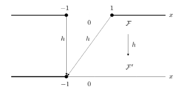
Figure 1: Example 1: Feasible sets, $\mathcal{F}$ and ${\mathcal{F}}^{\prime}$, and mapping $h$.

Example 2.

Let us consider the optimization problem

$$\min_{x_{1}\in{\mathbb{R}},x_{2}\in{\mathbb{R}}}\quad f(x_{1},x_{2})=x_{1}^{2}+x_{1}x_{2}^{2}$$ (6)

$${\rm{s}}{\rm{.t}}.\quad\Phi_{1}(x_{1},x_{2})=1-x_{1}x_{2}^{2}\leq 0,1-x_{1}\leq 0$$

where ${\mathcal{D}}={\mathbb{R}}^{2}$, and $x_{1},x_{2}\in{\mathbb{R}}$ are decision variables. For this problem, the constrained optimal solution is $x_{1}^{*}=x_{2}^{*}=1$, the corresponding primal optimal value is $p^{*}=f(x^{*})=2$, and the corresponding feasible set is

$${\mathcal{F}}:= \{(x_{1},x_{2})\in{\mathbb{R}}^{2}:\Phi_{1}(x)\leq 0,\Phi_{2}(x)\leq 0\}$$

$$= \{(x_{1},x_{2})\in{\mathbb{R}}^{2}:x_{1}\geq 1,x_{1}x_{2}^{2}\geq 1\},$$

which is non-convex as shown in Figure 2.

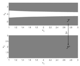
Figure 2: Example 2. Feasible sets, $\mathcal{F}$ and ${\mathcal{F}}^{\prime}$, and mapping $h$.

Now, let us consider the mapping

$$x=\left[{\begin{array}[]{*{20}c}{x_{1}}\\ {x_{2}}\\ \end{array}}\right]\mapsto h\left({\left[{\begin{array}[]{*{20}c}{x_{1}}\\ {x_{2}}\\ \end{array}}\right]}\right)=\left[{\begin{array}[]{*{20}c}{x_{1}}\\ {x_{1}x_{2}^{2}}\\ \end{array}}\right],$$

and the corresponding change of variables

$$v=\left[{\begin{array}[]{*{20}c}{v_{1}}\\ {v_{2}}\\ \end{array}}\right]=h\left({\left[{\begin{array}[]{*{20}c}{x_{1}}\\ {x_{2}}\\ \end{array}}\right]}\right)=\left[{\begin{array}[]{*{20}c}{x_{1}}\\ {x_{1}x_{2}^{2}}\\ \end{array}}\right].$$

Using this transformation, a convexification is given by

$$\min_{v_{1}\in{\mathbb{R}},v_{2}\in{\mathbb{R}}}\quad f^{\prime}(v_{1},v_{2})=v_{1}^{2}+v_{2}$$ (7)

$${\rm{s}}{\rm{.t}}.\quad\Phi_{1}^{\prime}(v_{1},v_{2})=1-v_{2}\leq 0,\quad\Phi_{2}^{\prime}(v_{1},v_{2})=1-v_{1}\leq 0,$$

where $h({\mathcal{D}})=h({\mathbb{R}}^{2})={\mathbb{R}}^{2}$. The corresponding optimal solution is $v_{1}^{*}=v_{2}^{*}=1$, and the corresponding feasible set is

$${\mathcal{F}}^{\prime}= \{(v_{1},v_{2})\in{\mathbb{R}}^{2}:\Phi_{1}^{\prime}(v)\leq 0,\Phi_{2}^{\prime}(v)\leq 0\}$$

$$= \{(v_{1},v_{2})\in{\mathbb{R}}^{2}:v_{1}\geq 1,v_{2}\geq 1\},$$

which is convex. Over $(v_{1},v_{2})\in{\mathcal{F}}^{\prime}$, $v_{1}\geq 1$ is invertible, and he inverse mapping, $h^{-1}:{\mathcal{F}}^{\prime}\to{\mathcal{F}}$, is given by

$$h^{-1}(v)=q(v)\left({\left[{\begin{array}[]{*{20}c}{v_{1}}\\ {v_{2}}\\ \end{array}}\right]}\right)=\left[{\begin{array}[]{*{20}c}{v_{1}}\\ {v_{2}/v_{1}}\\ \end{array}}\right]=\left[{\begin{array}[]{*{20}c}{x_{1}}\\ {x_{2}}\\ \end{array}}\right].$$

Therefore, $h:{\mathcal{F}}\to{\mathcal{F}}^{\prime}$ is a bijection (hence, a surjection), and, (7) is a lossless convexification of (6) by Definition 4.

An implication of Definition 4 is that solutions of 3 have a surjective correspondence to solutions of 1. Therefore, even if 1 is nonconvex, its solutions can be found from the convex 3. Moreover, another property is that the existence of such a lossless convexification ensures strong duality of the original 1 (with the Slater’s condition). This result will be presented in the next subsection.

3.2 Strong duality

In this subsection, we investigate a relation between the lossless convexification and strong duality. Some preliminary definitions are first introduced below. Associated with 1, define the set

$${\mathcal{G}}:= \{(\Phi_{1}(x),\Phi_{2}(x),\ldots,\Phi_{N}(x),f(x))$$

$$\in{\mathbb{S}}^{n}\times{\mathbb{S}}^{n}\times\cdots\times{\mathbb{S}}^{n}\times{\mathbb{R}}:x\in{\mathcal{D}}\},$$

which is called the graph of the constrained optimization problem in 1. The corresponding epigraph form [1] is defined as

$${\mathcal{A}}:= \{(\bar{U},t):\nexists x\in{\mathcal{D}},\Phi_{i}(x)\preceq U_{i},i\in\{1,2,\ldots,N\},$$

$$f(x)\leq t\}.$$ (8)

where $\bar{U}:=(U_{1},U_{2},\ldots,U_{N})$. Note that $\mathcal{A}$ includes all the points in $\mathcal{G}$, as well as points that are ‘worse,’ i.e., those with larger objective or inequality constraint function values [1]. In other words, ${\mathcal{A}}$ can be also expressed as

$${\mathcal{A}}={\mathcal{G}}+(\underbrace{{\mathbb{S}}_{+}^{n}\times{\mathbb{S}}_{+}^{n}\times\cdots{\mathbb{S}}_{+}^{n}}_{N-{\rm{times}}}\times R_{+}),$$

where ${\mathbb{R}}_{+}$ is the set of nonnegative real numbers and ‘$+$’ above is Minkowski sum. Similarly, for the convexified problem in 3, we define the graph and epigraph form as

$${\mathcal{G}}^{\prime}:= \{(\Phi_{1}^{\prime}(x),\Phi_{2}^{\prime}(x),\ldots,\Phi_{N}^{\prime}(x),f^{\prime}(x))$$

$$\in{\mathbb{S}}^{\hat{n}}\times{\mathbb{S}}^{\hat{n}}\times\cdots\times{\mathbb{S}}^{\hat{n}}\times{\mathbb{R}}:x\in{\mathcal{D}}\},$$

and

$${\mathcal{A}}^{\prime}:= \{(\bar{U},t):\exists v\in h(D),$$

$$\Phi_{i}^{\prime}(v)\preceq U_{i},i\in\{1,2,\ldots,N\},f^{\prime}(v)\leq t\}$$

respectively. Note that since $\Phi_{i}^{\prime},i\in\{1,2,\ldots,N\}$, and $f^{\prime}$ are convex, so is ${\mathcal{A}}^{\prime}$ as well. Now, we are in position to present the main result.

Theorem 1 (Strong duality).

Suppose that 3 is a lossless convexification of 1. If 1 satisfies the Slater’s condition, then strong duality holds for 1.

Proof.

Suppose that 3 is a lossless convexification of 1, and 1 satisfies the Slater’s condition. By definition, the primal optimal value satisfies

$$p^{*}=\inf\{t\in{\mathbb{R}}:(\underbrace{0,0,\ldots,0}_{N-{\rm{times}}},t)\in{\mathcal{A}}\},$$

where $0$ denotes a zero matrix with compatible dimensions.

Using the fact that $h:{\mathcal{F}}\to{\mathcal{F}}^{\prime}$ is a surjection, we can prove the following claim.

Claim 1.

We have

$$p^{*}= \inf\{t\in{\mathbb{R}}:(\underbrace{0,0,\ldots,0}_{N-{\rm{times}}},t)\in{\mathcal{A}}\}$$

$$= \inf\{t\in{\mathbb{R}}:(\underbrace{0,0,\ldots,0}_{N-{\rm{times}}},t)\in{\mathcal{A}}^{\prime}\},$$

where $0$ denotes a zero matrix with compatible dimensions.

Proof of Claim 1: We will prove the following identity: $\{t\in{\mathbb{R}}:(0,t)\in{\mathcal{A}}\}=\{t\in{\mathbb{R}}:(0,t)\in{\mathcal{A}}^{\prime}\}$. Suppose that $(0,t)\in{\mathcal{A}}$, i.e., $\Phi_{i}(x)\preceq 0,f(x)\leq t$ holds for some $x\in{\mathcal{D}}$. Then, $\Phi_{i}^{\prime}(h(x))=\Phi_{i}^{\prime}(v)\preceq 0,f^{\prime}(h(x))=f^{\prime}(v)\leq t$ also holds. This implies that $(0,t)\in{\mathcal{A}}^{\prime}$ holds. On the other hand, suppose $\Phi_{i}^{\prime}(v)\preceq 0,f^{\prime}(v)\leq t$ holds for some $v\in h({\mathcal{D}})$. Then, since $h:{\mathcal{F}}\to{\mathcal{F}}^{\prime}$ is a surjection, there exists a mapping, $q:{\mathcal{F}}^{\prime}\to{\mathcal{F}}$, such that $h(q(v))=v$, and hence, it follows that

$$\Phi_{i}^{\prime}(v)=\Phi_{i}^{\prime}((h\circ q)(v))=(\Phi_{i}^{\prime}\circ h)(q(v))=\Phi_{i}(x)\preceq 0,$$

and

$$f^{\prime}(v)=f^{\prime}((h\circ q)(v))=(f^{\prime}\circ h)(q(v))=f(x)\leq t.$$

Therefore, $\{t\in{\mathbb{R}}:(0,t)\in{\mathcal{A}}\}=\{t\in{\mathbb{R}}:(0,t)\in{\mathcal{A}}^{\prime}\}$, and hence $p^{*}=\inf\{t\in{\mathbb{R}}:(0,t)\in{\mathcal{A}}\}=\inf\{t\in{\mathbb{R}}:(0,t)\in{\mathcal{A}}^{\prime}\}$. This completes the proof. $\blacksquare$

Using similar arguments, we can also prove the following key result.

Claim 2.

Let us divide ${\mathcal{A}}$ into the two sets

$${\mathcal{A}}_{1}:=\{(\bar{U},t)\in{\mathcal{A}}:U_{i}\preceq 0,i\in\{1,2,\ldots,N\}\}$$

and

$${\mathcal{A}}_{2}:=\{(\bar{U},t)\in{\mathcal{A}}:U_{i}\npreceq 0,i\in\{1,2,\ldots,N\}\},$$

so that ${\mathcal{A}}_{1}\cup{\mathcal{A}}_{2}={\mathcal{A}}$. Moreover, divide ${\mathcal{A}}^{\prime}$ into the two sets

$${\mathcal{A}}_{1}^{\prime}:=\{(\bar{U},t)\in{\mathcal{A}}^{\prime}:U_{i}\preceq 0,i\in\{1,2,\ldots,N\}\}$$

and

$${\mathcal{A}}_{2}^{\prime}:=\{(\bar{U},t)\in{\mathcal{A}}^{\prime}:U_{i}\npreceq 0,i\in\{1,2,\ldots,N\}\}$$

so that ${\mathcal{A}}_{1}^{\prime}\cup{\mathcal{A}}_{2}^{\prime}={\mathcal{A}}^{\prime}$. Then, the following statements hold true:

1. ${\mathcal{A}}_{1}={\mathcal{A}}_{1}^{\prime}$,

2. ${\mathcal{A}}_{2}\subseteq{\mathcal{A}}_{2}^{\prime}$,

3. ${\mathcal{A}}\subseteq{\mathcal{A}}^{\prime}$.

Proof of Claim 2: We first prove the identity ${\mathcal{A}}_{1}={\mathcal{A}}_{1}^{\prime}$. This part is similar to the proof of Claim 1. Suppose that $U_{i}\preceq 0,i\in\{1,2,\ldots,N\}$ holds, and $(\bar{U},t)\in{\mathcal{A}}$, i.e., $\Phi_{i}(x)\preceq U_{i},f(x)\leq t$ holds for some $x\in{\mathcal{D}}$. Then, $\Phi_{i}^{\prime}(h(x))=\Phi_{i}^{\prime}(v)\preceq U_{i},f^{\prime}(h(x))=f^{\prime}(v)\leq t$ also holds. This implies that $(\bar{U},t)\in{\mathcal{A}}^{\prime}$ holds. On the other hand, suppose $\Phi_{i}^{\prime}(v)\preceq U_{i}\preceq 0,f^{\prime}(v)\leq t$ holds for some $v\in h({\mathcal{D}})$. Then, since $h:{\mathcal{F}}\to{\mathcal{F}}^{\prime}$ is a surjection, there exists a mapping, $q:{\mathcal{F}}^{\prime}\to{\mathcal{F}}$, such that $h(q(v))=v$, and hence, it follows that

$$\Phi_{i}^{\prime}(v)=\Phi_{i}^{\prime}((h\circ q)(v))=(\Phi_{i}^{\prime}\circ h)(q(v))=\Phi_{i}(x)\preceq U_{i},$$

and

$$f^{\prime}(v)=f^{\prime}((h\circ q)(v))=(f^{\prime}\circ h)(q(v))=f(x)\leq t.$$

Therefore, ${\mathcal{A}}_{1}={\mathcal{A}}_{1}^{\prime}$ holds.

On the other hand, if $U_{i}\npreceq 0,i\in\{1,2,\ldots,N\}$, then ${\mathcal{A}}_{2}\subseteq{\mathcal{A}}_{2}^{\prime}$ is satisfied. In particular, suppose that $\Phi_{i}(x)\preceq U_{i},f(x)\leq t$ holds for some $x\in{\mathcal{D}}$. Then, $\Phi_{i}^{\prime}(h(x))=\Phi_{i}^{\prime}(v)\preceq U_{i},f^{\prime}(h(x))=f^{\prime}(v)\leq t$ also holds. Therefore, $(\bar{U},t)\in{\mathcal{A}}^{\prime}$, which implies ${\mathcal{A}}_{2}\subseteq{\mathcal{A}}_{2}^{\prime}$. The reverse does not hold in general. To see it, suppose $\Phi_{i}^{\prime}(v)\preceq U_{i},f^{\prime}(v)\leq t$ holds for some $v\in h({\mathcal{D}})$. Then, since there is no guarantee that $h:{\mathcal{F}}\to{\mathcal{F}}^{\prime}$ is a surjection when $U_{i}\npreceq 0,i\in\{1,2,\ldots,N\}$, we cannot ensure that there exists $x$ such that $\Phi_{i}(x)\preceq U_{i},f(x)\leq t$. The statement 3) is implied by the statement 1) and statement 2). This completes the proof. $\blacksquare$

Next, let us return to our main concern. To prove Theorem 1, we define the set

$${\mathcal{B}}:=\{(0,s):s<p^{*}\}.$$

Since ${\mathcal{A}}^{\prime}$ and $\mathcal{B}$ are convex, there exists a separating hyperplane that separates $\mathcal{A}^{\prime}$ and $\mathcal{B}$ by the separating hyperplane theorem in [1, sec. 2.5], as shown in Figure 3.

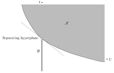
Figure 3: Two convex sets, ${\mathcal{A}}^{\prime}$ (shaded region) and $\mathcal{B}$, and a separating hyperplane.

In particular, the existence of a separating hyperplane implies that there exists $(\bar{\Lambda},\mu)\neq 0$ and $\alpha\in{\mathbb{R}}$ such that

$$(\bar{U},t)\in{\mathcal{A}}^{\prime}\Rightarrow\sum\limits_{i=1}^{N}{Tr(\Lambda_{i}U_{i})}+\mu t\geq\alpha$$ (9)

and

$$(\bar{U},t)\in{\mathcal{B}}\Rightarrow\sum\limits_{i=1}^{N}{Tr(\Lambda_{i}U_{i})}+\mu t\leq\alpha.$$

Using the inclusion ${\mathcal{A}}\subseteq{\mathcal{A}}^{\prime}$ in Claim 2, it follows from (9) that

$$(\bar{U},t)\in{\mathcal{A}}\Rightarrow\sum\limits_{i=1}^{N}{Tr(\Lambda_{i}U_{i})}+\mu t\geq\alpha$$ (10)

and

$$(\bar{U},t)\in{\mathcal{B}}\Rightarrow\sum\limits_{i=1}^{N}{Tr(\Lambda_{i}U_{i})}+\mu t\leq\alpha$$ (11)

From (10), we conclude that $\Lambda_{i}\succeq 0,i\in\{1,2,\ldots,N\}$ and $\mu\geq 0$. Otherwise $\sum\limits_{i=1}^{N}{Tr(\Lambda_{i}U_{i})}+\mu t$ is unbounded below over ${\mathcal{A}}$, contradicting (10). The condition (11) simply means that $\mu t\leq\alpha$ (since $\bar{U}=0$) for all $t<p^{*}$, and hence, $\mu p^{*}\leq\alpha$. Together with (10), we conclude that for any $x\in\mathcal{D}$

$$\sum\limits_{i=1}^{N}{Tr(\Lambda_{i}\Phi_{i}(x))}+\mu f(x)\geq\alpha\geq\mu p^{*}$$ (12)

Assume that $\mu>0$. In that case we can divide (12) by $\mu$ to obtain

$$L\left({x,\frac{{\bar{\Lambda}}}{\mu}}\right)=\sum\limits_{i=1}^{N}{Tr\left({\Phi_{i}(x)\frac{{\Lambda_{i}}}{\mu}}\right)}+f(x)\geq p^{*}$$

for all $x\in\mathcal{D}$, from which it follows, by minimizing over $x$, that $g\left({\frac{\bar{\Lambda}}{{\mu}}}\right)\geq p^{*}$. By weak duality we have $g\left({\frac{\bar{\Lambda}}{{\mu}}}\right)\leq p^{*}$, so in fact $g\left({\frac{\bar{\Lambda}}{{\mu}}}\right)=p^{*}$. This shows that strong duality holds, and that the dual optimum is attained, at least in the case when $\mu>0$.

Now consider the case $\mu=0$. From (10), we conclude that for all $x\in\mathcal{D}$,

$$\sum\limits_{i=1}^{N}{Tr(\Lambda_{i}\Phi_{i}(x))}\geq 0$$

Assume that $\tilde{x}$ is the point that satisfies the Slater condition, i.e., $\Phi_{i}(\tilde{x})\prec 0,i\in\{1,2,\ldots,N\}$. Then, we have $\sum\limits_{i=1}^{N}{Tr(\Lambda_{i}\Phi_{i}(\tilde{x}))}\geq 0$. Since $\Phi_{i}(\tilde{x})<0,i\in\{1,2,\ldots,N\}$ and $\Lambda\succeq 0$, we conclude that $\Lambda_{i}=0,i\in\{1,2,\ldots,N\}$. Therefore, $\Lambda_{i}=0,i\in\{1,2,\ldots,N\}$ and $\mu=0$, which contradicts $(\bar{\Lambda},\mu)\neq 0$. Intuition of the overall ideas are illustrated in Figure 4. ${\mathcal{A}}^{\prime}$ is convex, while $\mathcal{A}$ may not be in general. $\mathcal{A}$ and ${\mathcal{A}}^{\prime}$ are identical over $U_{i}\preceq 0,i\in\{1,2,\ldots,N\}$, while ${\mathcal{A}}^{\prime}$ includes $\mathcal{A}$ when $U_{i}\npreceq 0,i\in\{1,2,\ldots,N\}$. Overall, the boundary of ${\mathcal{A}}^{\prime}$ is a convex envelope of $\mathcal{A}$, and both ${\mathcal{A}}^{\prime}$ and ${\mathcal{A}}$ share the same separating hyperplane.

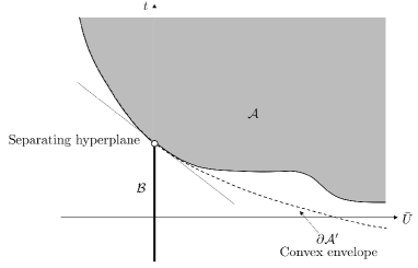
Figure 4: Sets $\mathcal{A}$ (shaded region), $\mathcal{B}$, the separating hyperplane, and the boundary of ${\mathcal{A}}^{\prime}$ (dashed line), denoted by $\partial{\mathcal{A}}^{\prime}$

In the sequel, several examples are given to illustrate the ideas of Theorem 1.

Example 3.2.

Let us consider Example 1 again. The optimization in (4) satisfies the Slater’s condition because with $x=2$, we have $\Phi_{1}(x)=-3<0$. Moreover, (4) a lossless convexification in (5). Therefore, strong duality holds by Theorem 1. To prove it directly, consider the corresponding Lagrangian function

$$L(x,\lambda)=x^{2}+\lambda(-x^{2}+1),$$

where $\lambda\geq 0$ is the Lagrangian multiplier, and the dual function

$$g(\lambda)= \inf_{x\in{\mathbb{R}}}L(x,\lambda)$$

$$= \inf_{x\in{\mathbb{R}}}\{x^{2}+\lambda(-x^{2}+1)\}.$$

To obtain a more explicit form of the dual function, one can observe that this dual function is bounded below in $x$ only when $\lambda\leq 1$. For $\lambda>1$, we have $g(\lambda)$ unbounded below in $x$. Therefore, we can conclude that the dual function is

$$g(\lambda)=\left\{{\begin{array}[]{*{20}c}{-\infty,\quad{\rm{if}}\,\,\lambda>1}\\ {\lambda,\quad{\rm{if}}\,\,0\leq\lambda\leq 1}\\ \end{array}}\right.$$

Then, the corresponding dual optimal value is $d^{*}=\sup_{\lambda\geq 0}g(\lambda)=1=p^{*}$. Therefore, strong duality holds.

Example 3.3.

Let us consider Example 2 again. The optimization (6) satisfies the Slater’s condition because with $x_{1}=2$ and $x_{2}=1$, we have $\Phi_{1}(x_{1},x_{2})=-3<0,\Phi_{1}(x_{1},x_{2})=-1<0$. Moreover, (6) admits the lossless convexification (7). Therefore, by Theorem 1, strong duality holds for (6). The corresponding Lagrangian function is

$$L(x,\bar{\Lambda})=x_{1}^{2}+x_{1}x_{2}^{2}+\lambda_{1}(1-x_{1}x_{2}^{2})+\lambda_{2}(1-x_{1}),$$

where $\bar{\Lambda}=(\lambda_{1},\lambda_{2})$ is the Lagrangian multipliers or the dual variables. Let us manually check if strong duality really holds. The dual function is given by

$$g(\bar{\Lambda})= \inf_{x_{1}\in{\mathbb{R}},x_{2}\in{\mathbb{R}}}L(x,\bar{\Lambda})$$

$$= \inf_{x_{1}\in{\mathbb{R}},x_{2}\in{\mathbb{R}}}\{x_{1}^{2}+x_{1}x_{2}^{2}+\lambda_{1}(1-x_{1}x_{2}^{2})+\lambda_{2}(1-x_{1})\}$$

$$= \inf_{x_{1}\in{\mathbb{R}},x_{2}\in{\mathbb{R}}}\{x_{1}^{2}-\lambda_{2}x_{1}+(1-\lambda_{1})x_{1}x_{2}^{2}+\lambda_{1}+\lambda_{2}\}.$$

To obtain an explicit form of the dual function, we first find extrema of $L(x,\bar{\Lambda})$ by checking the following first-order optimality conditions:

$$\frac{d}{{dx_{1}}}\{x_{1}^{2}-\lambda_{2}x_{1}+(1-\lambda_{1})x_{1}x_{2}+\lambda_{1}+\lambda_{2}\}$$

$$= 2x_{1}-\lambda_{2}+(1-\lambda_{1})x_{2}^{2}$$

$$= 0$$ (13)

and

$$\frac{d}{{dx_{2}}}\{x_{1}^{2}-\lambda_{2}x_{1}+(1-\lambda_{1})x_{1}x_{2}^{2}+\lambda_{1}+\lambda_{2}\}$$

$$= 2(1-\lambda_{1})x_{1}x_{2}=0.$$ (14)

To satisfy (14), in the case $1-\lambda_{1}\neq 0$, we have $x_{1}=0$ or $x_{2}=0$. If $x_{1}=0$, then $x_{2}=\sqrt{\frac{{\lambda_{2}}}{{1-\lambda_{1}}}}$ provided that $1>\lambda_{1}$. Therefore, the dual function satisfies

$$\mathop{\sup}\limits_{\lambda_{1},\lambda_{2}\geq 0}g(\bar{\Lambda})= \mathop{\sup}\limits_{\lambda_{1},\lambda_{2}\geq 0}\left\{{x_{1}^{2}-\lambda_{2}x_{1}+(1-\lambda_{1})x_{1}x_{2}^{2}+\lambda_{1}+\lambda_{2}}\right\}$$

$$= \mathop{\sup}\limits_{\lambda_{1},\lambda_{2}\geq 0}\left\{{\lambda_{1}+\lambda_{2}:1>\lambda_{1}}\right\}$$

$$= \infty.$$

Therefore, this case is discarded. If $x_{2}=0$, then $x_{1}=\lambda_{2}/2$, and the dual problem is

$$\mathop{\sup}\limits_{\lambda_{1},\lambda_{2}\geq 0}g(\bar{\Lambda})= \mathop{\sup}\limits_{\lambda_{1},\lambda_{2}\geq 0}\left\{{x_{1}^{2}-\lambda_{2}x_{1}+(1-\lambda_{1})x_{1}x_{2}^{2}+\lambda_{1}+\lambda_{2}}\right\}$$

$$= \mathop{\sup}\limits_{\lambda_{1},\lambda_{2}\geq 0}\left\{{-\frac{{\lambda_{2}^{2}}}{4}+\lambda_{1}+\lambda_{2}:1-\lambda_{1}\neq 0}\right\}$$

$$= \infty.$$

Therefore, this case is also discarded, and $1-\lambda_{1}=0$ should be hold. In this case, we have

$$x_{1}=\frac{{\lambda_{2}}}{2},\quad x_{2}\in{\mathbb{R}},$$

and the corresponding dual problem is

$$\sup_{\lambda_{1},\lambda_{2}\geq 0}g(\bar{\Lambda})$$

$$= \sup_{\lambda_{1},\lambda_{2}\geq 0}\left\{{-\frac{{\lambda_{2}^{2}}}{4}+\lambda_{1}+\lambda_{2}:\,1-\lambda_{1}=0}\right\}$$

$$= 2,$$

whose optimal dual value is $d^{*}=2$. Therefore, $d^{*}=2=p^{*}$, and strong duality holds.

In this section, the notion of the lossless convexification has been introduced, and a relation between the lossless convexification and strong duality has been established. In the next section, we will present a formulation of the state-feedback problem, and prove the corresponding strong duality using the results in this paper.

4 State-feedback stabilization

In this section, we present a control problem where the proposed results can be applied.

4.1 Continuous-time case

Let us consider the continuous-time linear time-invariant (LTI) system

$$\dot{x}(t)=Ax(t)+Bu(t),\quad x(0)\in R^{n},$$

where $A\in{\mathbb{R}}^{n\times n}$, $B\in{\mathbb{R}}^{n\times m}$, $t\geq 0$ is the time, $x(t)\in{\mathbb{R}}^{n}$ is the state vector, and $u(t)\in{\mathbb{R}}^{m}$ is the input vector. One of the most fundamental problems for this LTI system is the state-feedback stabilization problem, which is designing a state-feedback control input, $u(t)=Fx(t)$, where $F\in{\mathbb{R}}^{m\times n}$ is called the state-feedback gain matrix, such that the closed-loop system, $\dot{x}(t)=Ax(t)+Bu(t)=(A+BF)x(t)$, is asymptotically stable [21]. Equivalently, the state-feedback problem can be formally written as follows.

Problem 4.4 (State-feedback stabilization problem).

Find a state-feedback gain $F\in{\mathbb{R}}^{m\times n}$ such that $A+BF$ is Hurwitz.

The state-feedback problem can be formulated as the feasibility problem with matrix inequalities (Lyapunov inequalities)

$$P\succeq\varepsilon I,\quad(A+BF)^{T}P+P(A+BF)\preceq-\varepsilon I,$$

where $P\in{\mathbb{S}}^{n}$ is called the Lyapunov matrix, $\varepsilon>0$ is some fixed sufficiently small number, and the second inequality is non-convex (bilinear in the decision variables $F$ and $P$), i.e., the feasible set of the second inequality may be non-convex in general. Here, the bilinear inequality is a special case of non-convexity inequalities, and implies that it is linear if the other variable is fixed, and vice versa. From standard results of linear system theory [22], the condition is equivalent to

$$P\succeq\varepsilon I,\quad(A+BF)P+P(A+BF)^{T}\preceq-\varepsilon I$$ (15)

because the eigenvalues of $A+BF$ are identical to the eigenvalues of $(A+BF)^{T}$ by duality. The corresponding feasibility problem in 1 can be converted to the equivalent optimization

$$\min_{P\in{\mathbb{S}}^{n},F\in{\mathbb{R}}^{m\times n}}\,\,\quad 0$$ (16)

$${\rm{s}}.{\rm{t}}.\quad\Phi_{1}(x)=(A+BF)P+P(A+BF)^{T}+\varepsilon I\preceq 0$$

$$\Phi_{2}(x)=\varepsilon I-P\preceq 0,$$

where

$$x=\left[{\begin{array}[]{*{20}c}P\\ F\\ \end{array}}\right].$$

Note that the feasibility problem in (15) is equivalent to the optimization in (16) in the sense that their solutions are identical. We consider the optimization form in (16) to fit the problem into the optimization form in 1, and this it not more than formality. Next, consider the mapping

$$x=\left[{\begin{array}[]{*{20}c}P\\ F\\ \end{array}}\right]\mapsto h\left({\left[{\begin{array}[]{*{20}c}P\\ F\\ \end{array}}\right]}\right)=\left[{\begin{array}[]{*{20}c}P\\ {FP}\\ \end{array}}\right],$$

and the corresponding change of variables

$$v=\left[{\begin{array}[]{*{20}c}P\\ M\\ \end{array}}\right]=h\left({\left[{\begin{array}[]{*{20}c}P\\ F\\ \end{array}}\right]}\right)=\left[{\begin{array}[]{*{20}c}P\\ {FP}\\ \end{array}}\right].$$

Using this transformation, a convexification of (16) is

$$\min_{P\in{\mathbb{S}}^{n},M\in{\mathbb{R}}^{m\times n}}\,\,\quad 0$$

$${\rm s.t.}\quad\Omega_{1}^{\prime}(v)=(AP+BM)+(AP+BM)^{T}+\varepsilon I\preceq 0,$$

$$\Omega_{2}^{\prime}(v)=\varepsilon I-P\preceq 0.$$

Over the feasible sets, ${\mathcal{F}}$ and ${\mathcal{F}}^{\prime}$, $P$ is nonsingular. Therefore, $h:{\mathcal{F}}\to{\mathcal{F}}^{\prime}$ is a bijection (and hence, a surjection), and the inverse mapping is given by

$$h^{-1}\left({\left[{\begin{array}[]{*{20}c}P\\ M\\ \end{array}}\right]}\right)=\left({\left[{\begin{array}[]{*{20}c}P\\ {MP^{-1}}\\ \end{array}}\right]}\right),$$

where $\left[{\begin{array}[]{*{20}c}P\\ M\\ \end{array}}\right]\in{\mathcal{F}}^{\prime}$. Therefore, (16) is initially nonconvex, but can be convexified using some transformations and manipulations. Lastly, we can prove that the original problem in (16) satisfies the Slater’s condition under a mild assumption, and hence, it satisfies strong duality by Theorem 1.

Claim 3.

Suppose that $(A,B)$ is stabilizable. Then, there exists a sufficiently small $\varepsilon>0$, $P\in{\mathbb{S}}^{n}$ and $F\in{\mathbb{R}}^{m\times n}$ such that

$$(A+BF)P+P(A+BF)^{T}+\varepsilon I\preceq 0,\quad\varepsilon I-P\preceq 0.$$ (17)

Proof 4.5.

It is clear from Lyapunov theory [22, 21] that if $(A,B)$ is stabilizable, then there exists $P\succ 0$ and $F\in{\mathbb{R}}^{m\times n}$ such that $(A+BF)P+P(A+BF)^{T}\prec 0$. Then, there always exists a sufficiently small $\varepsilon>0$ such that (17) is satisfied. Therefore, the proof is completed.

By Claim 3, the optimization (16) admits a strictly feasible solution. This is because for the feasible $\varepsilon>0$ that satisfies (17), we can divide it by $2$, and then with this $\varepsilon$, the inequalities in (16) are satisfied with strict inequalities. In conclusion, the original problem (16) satisfies strong duality by Theorem 1.

Now, let us consider the output vector

$$y(t)=Cx(t)\in{\mathbb{R}}^{p},$$

where $C\in{\mathbb{R}}^{p\times n}$ is the output matrix. The static output-feedback control problem is designing a static output-feedback control input, $u(t)=Fy(t)$, where $F\in{\mathbb{R}}^{m\times p}$ is called the static output-feedback gain matrix, such that the closed-loop system, $\dot{x}(t)=Ax(t)+Bu(t)=(A+BFC)x(t)$, is asymptotically stable [21]. This problem is formally stated in the following.

Problem 4.6 (Static output-feedback stabilization).

Find a feedback gain $F\in{\mathbb{R}}^{m\times p}$ such that $A+BFC$ is Hurwitz.

The static output-feedback problem is much more challenging than the state-feedback problem, and is known to be non-convex and NP-hard [7, 8, 9]. Using Lyapunov theory again, it can be rewritten by the non-convex optimization

$$\min_{P\in{\mathbb{S}}^{n},F\in{\mathbb{R}}^{m\times p}}\,\,\quad 0$$ (18)

$${\rm{s}}.{\rm{t}}.\quad\Phi_{1}(x)=(A+BFC)P+P(A+BFC)^{T}+\varepsilon I\preceq 0,$$

$$\Phi_{2}(x)=\varepsilon I-P\preceq 0,$$

where

$$x=\left[{\begin{array}[]{*{20}c}P\\ F\\ \end{array}}\right].$$

Due to the matrix $C$, it is hard to find a lossless convexification in general. This is because, the matrix $C$ is not invertible, and it separates matrices $F$ and $P$. Therefore, it is hard to guarantee strong duality for (18).

4.2 Discrete-time case

Consider the discrete-time linear time-invariant (LTI) system

$$x(k+1)=Ax(k)+Bu(k),\quad x(0)\in{\mathbb{R}}^{n},$$

where $A\in{\mathbb{R}}^{n\times n}$, $B\in{\mathbb{R}}^{n\times m}$, the integer $k\geq 0$ is the time, $x(k)\in{\mathbb{R}}^{n}$ is the state vector, and $u(k)\in{\mathbb{R}}^{m}$ is the input vector. As in the continuous-time case, the corresponding state-feedback stabilization problem is stated below.

Problem 4.7 (State-feedback stabilization problem).

Find a feedback gain $F\in{\mathbb{R}}^{m\times n}$ such that $A+BF$ is Schur.

The problem can be formulated as the Lyapunov inequality

$$P\succeq\varepsilon I,\quad(A+BF)^{T}P(A+BF)-P\preceq-\varepsilon I,$$

where $P\in{\mathbb{S}}^{n}$ is called the Lyapunov matrix, and the second inequality is in general non-convex. Moreover, by duality of LTI systems again, it can be equivalently written As

$$P\succeq\varepsilon I,\quad(A+BF)P(A+BF)^{T}-P\preceq-\varepsilon I.$$

The problem in can be converted to the equivalent optimization

$$\inf_{P\in{\mathbb{S}}^{n},F\in{\mathbb{R}}^{m\times n}}0$$ (19)

$${\rm s.t.}\quad(A+BF)P(A+BF)^{T}-P+\varepsilon I=\Phi_{1}(x)\preceq 0,$$

$$\varepsilon I-P=\Phi_{2}(x)\preceq 0$$

where

$$x=\left[{\begin{array}[]{*{20}c}P\\ F\\ \end{array}}\right].$$

Consider the mapping

$$x=\left[{\begin{array}[]{*{20}c}P\\ F\\ \end{array}}\right]\mapsto h\left({\left[{\begin{array}[]{*{20}c}P\\ F\\ \end{array}}\right]}\right)=\left[{\begin{array}[]{*{20}c}P\\ {FP}\\ \end{array}}\right]$$

and the corresponding change of variables

$$v=\left[{\begin{array}[]{*{20}c}P\\ M\\ \end{array}}\right]=h\left({\left[{\begin{array}[]{*{20}c}P\\ F\\ \end{array}}\right]}\right)=\left[{\begin{array}[]{*{20}c}P\\ {FP}\\ \end{array}}\right].$$

Using this transformation, a convexification is

$$\inf_{P\in{\mathbb{S}}^{n},M\in{\mathbb{R}}^{m\times n}}0$$ (20)

$${\rm s.t.}\quad(AP+BM)P^{-1}(AP+BM)^{T}-P+\varepsilon I=\Phi_{1}^{\prime}(v)\preceq 0,$$

$$\varepsilon I-P=\Phi_{2}^{\prime}(v)\preceq 0.$$

The domain of $\Phi_{1}^{\prime}$ is $\{(P,M)\in{\mathbb{S}}^{n}\times{\mathbb{R}}^{m\times n}:P\succ 0\}$. Over the domain, we can prove that $\Phi_{1}^{\prime}(v)\preceq 0$ is convex. To prove it, one can check the convexity of the interior

$${\bf int}({\mathcal{F}}):= \{(P,M)\in{\mathbb{S}}^{n}\times{\mathbb{R}}^{m\times n}:P\succ\varepsilon I,$$

$$(AP+BM)P^{-1}(AP+BM)^{T}-P+\varepsilon I\prec 0\},$$

where ${\bf int}$ denotes the interior. Note that the set ${\bf int}({\mathcal{F}})$ is convex because after taking the Schur complement [3], it is equivalently expressed as

$${\bf int}({\mathcal{F}}):= \{(P,M)\in{\mathbb{S}}^{n}\times{\mathbb{R}}^{m\times n}:P\succ\varepsilon I,$$

$$\left.{\left[{\begin{array}[]{*{20}c}{-P+\varepsilon I}&{(AP+BM)}\\ {(AP+BM)^{T}}&{-P}\\ \end{array}}\right]\prec 0}\right\},$$

which is convex. In conclusion, (19) is initially a nonconvex bilinear matrix inequality problem, but can be convexified using some transformations and manipulations. Moreover, $P$ is nonsingular in ${\mathcal{F}}$ and ${\mathcal{F}}^{\prime}$. Therefore, $h$ is a bijection, and the inverse mapping is given by

$$h^{-1}\left({\left[{\begin{array}[]{*{20}c}P\\ M\\ \end{array}}\right]}\right)=\left[{\begin{array}[]{*{20}c}P\\ {MP^{-1}}\\ \end{array}}\right].$$

By Definition 4, (20) is a lossless convexification of (19). Lastly, we can prove that the original problem in (16) satisfies the Slater’s condition under a mild assumption.

Claim 4.

Suppose that $(A,B)$ is stabilizable. Then, there exists a sufficiently small $\varepsilon>0$, $P\in{\mathbb{S}}^{n}$ and $F\in{\mathbb{R}}^{m\times n}$ such that

$$(A+BF)P(A+BF)^{T}-P\prec-\varepsilon I,\quad\varepsilon I-P\prec 0.$$

Proof 4.8.

It is clear from Lyapunov theory [22, 21] that if $(A,B)$ is stabilizable, then there exists $P\succ 0$ and $F\in{\mathbb{R}}^{m\times n}$ such that $(A+BF)P(A+BF)^{T}-P\prec 0$. Therefore, the proof is completed.

Therefore, (19) admits a strictly feasible solution, and satisfies the Slater’s condition. By Theorem 1, the problem in (4.4) satisfies strong duality.

Finally, the static output-feedback stabilization problem for discrete-time systems is omitted here for brevity, but this problem can be addressed in similar ways as in the continuous-time cases.

Conclusion

In this paper, we have studied strong duality of non-convex semidefinite programming problems (SDPs). It turns out that a class of non-convex SDPs with special structures satisfies strong duality under the Slater’s condition. Examples have been given to illustrate the proposed results. We expect that the proposed analysis can potentially deepen our understanding of non-convex SDPs arising in control communities, and promote their analysis based on KKT conditions. In particular, the developed results can be used to reveal connections between several control-related results and SDP dualities as in [16]. Moreover, the results can be also applied to develop new algorithms for control designs, such as the static output-feedback design [23, 24, 10]. Another potential topic is to investigate strong duality of non-convex SDPs which can be convexified with several conversions of the problems using Schur complement [3] and its variations. These agendas can be potential future directions.

References

- [1] S. Boyd and L. Vandenberghe, Convex Optimization. Cambridge University Press, 2004.
- [2] L. Vandenberghe and S. Boyd, “Semidefinite programming,” SIAM review, vol. 38, no. 1, pp. 49–95, 1996.
- [3] S. Boyd, L. El Ghaoui, E. Feron, and V. Balakrishnan, Linear Matrix Inequalities in Systems and Control Theory. Philadelphia, PA: SIAM, 1994.
- [4] M. C. De Oliveira, J. Bernussou, and J. C. Geromel, “A new discrete-time robust stability condition,” Systems & control letters, vol. 37, no. 4, pp. 261–265, 1999.
- [5] J. C. Geromel, R. H. Korogui, and J. Bernussou, “ and robust output feedback control for continuous time polytopic systems,” Control Theory & Applications, IET, vol. 1, no. 5, pp. 1541–1549, 2007.
- [6] L. El Ghaoui and S.-I. Niculescu, Advances in linear matrix inequality methods in control. Siam, 2000, vol. 2.
- [7] M. Fu and Z.-Q. Luo, “Computational complexity of a problem arising in fixed order output feedback design,” Systems & Control Letters, vol. 30, no. 5, pp. 209–215, 1997.
- [8] M. Fu, “Pole placement via static output feedback is NP-hard,” IEEE Transactions on Automatic Control, vol. 49, no. 5, pp. 855–857, 2004.
- [9] V. Blondel and J. N. Tsitsiklis, “NP-hardness of some linear control design problems,” SIAM journal on control and optimization, vol. 35, no. 6, pp. 2118–2127, 1997.
- [10] J. C. Geromel, C. De Souza, and R. Skelton, “Static output feedback controllers: stability and convexity,” IEEE Transactions on Automatic Control, vol. 43, no. 1, pp. 120–125, 1998.
- [11] D. P. Bertsekas, Nonlinear programming. Athena scientific Belmont, 1999.
- [12] M. C. De Oliveira, J. C. Geromel, and J. Bernussou, “Extended and norm characterizations and controller parametrizations for discrete-time systems,” International Journal of Control, vol. 75, no. 9, pp. 666–679, 2002.
- [13] D. D. Yao, S. Zhang, and X. Y. Zhou, “Stochastic linear-quadratic control via semidefinite programming,” SIAM Journal on Control and Optimization, vol. 40, no. 3, pp. 801–823, 2001.
- [14] M. A. Rami and X. Y. Zhou, “Linear matrix inequalities, Riccati equations, and indefinite stochastic linear quadratic controls,” Automatic Control, IEEE Transactions on, vol. 45, no. 6, pp. 1131–1143, 2000.
- [15] D. Henrion, G. Meinsma et al., “Rank-one LMIs and Lyapunov’s inequality,” IEEE Transactions on Automatic Control, vol. 46, no. 8, pp. 1285–1288, 2001.
- [16] V. Balakrishnan and L. Vandenberghe, “Semidefinite programming duality and linear time-invariant systems,” IEEE Transactions on Automatic Control, vol. 48, no. 1, pp. 30–41, 2003.
- [17] D. Lee and J. Hu, “Primal-dual Q-learning framework for LQR design,” IEEE Transactions on Automatic Control, vol. 64, no. 9, pp. 3756–3763, 2018.
- [18] A. Gattami, “Generalized linear quadratic control,” IEEE Transactions on Automatic Control, vol. 55, no. 1, pp. 131–136, 2010.
- [19] S. You and J. C. Doyle, “A Lagrangian dual approach to the Generalized KYP lemma,” in CDC, 2013, pp. 2447–2452.
- [20] S. You, A. Gattami, and J. C. Doyle, “Primal robustness and semidefinite cones,” arXiv preprint arXiv:1503.07561, 2015.
- [21] H. K. Khalil, “Nonlinear systems,” Upper Saddle River, 2002.
- [22] C.-T. Chen, Linear System Theory and Design. Oxford University Press, Inc., 1995.
- [23] L. El Ghaoui, F. Oustry, and M. AitRami, “A cone complementarity linearization algorithm for static output-feedback and related problems,” IEEE Transactions on Automatic Control, vol. 42, no. 8, pp. 1171–1176, 1997.
- [24] C. A. Crusius and A. Trofino, “Sufficient LMI conditions for output feedback control problems,” IEEE Transactions on Automatic Control, vol. 44, no. 5, pp. 1053–1057, 1999.