Families of Skyrmions in Two-Dimensional Spin-1/2 Systems

Abstract

We find Skyrmion-like topological excitations for a two-dimensional spin-1/2 system. Expressing the spinor wavefunction in terms of a rotation operator maps the spin-1/2 system to a Manakov system. We employ both analytical and numerical methods to solve the resulting Manakov system. Using a generalized similarity transformation, we reduce the two-dimensional Manakov system to the integrable one-dimensional Manakov system. Solutions obtained in this manner diverge at the origin. We employ a power series method to obtain an infinite family of localized and nondiverging solutions characterized by a finite number of nodes. A numerical method is then used to obtain a family of localized oscillatory solutions with an infinite number of nodes corresponding to a skyrmion composed of concentric rings with intensities alternating between the two components of the spinor. We investigate the stability of the skyrmion solutions found here by calculating their energy functional in terms of their effective size. It turns out that indeed the skyrmion is most stable when the phase difference between the concentric rings is $\pi$, i.e., alternating between spin up and spin down. Our results are also applicable to doubly polarized optical pulses.

I Introduction

The vector non-linear Schrödinger equation (NLSE) describes spinor systems and the interaction between its field components. The model has also various applications in different areas of physics, for instance, the propagation of electromagnetic waves with arbitrary polarization in a self-focusing media [1], and the evolution of waves in plasma [2]. It is also shown [3] that the vector NLSE governs the average dynamics of dispersion-managed solitons which are considered as a key element for optical communication. The soliton robustness to polarisation-mode dispersion has a strong dependence on both chromatic dispersion and soliton energy [22]. It is known that the two-component vector NLSE or the Manakov system is completely integrable and is solvable by the inverse scattering transform (IST) method. Recently, Manakov spatial solitons were observed in AlGaAs planar waveguides [4]. More recently, the Si-based waveguides using similar phenomena are served as optical biosensors [23]. The similarity reductions of the 2D coupled NLSE have been studied by Lie’s method. It is shown that the 2D coupled NLSE is reduced to the 1D-NLSE by the similarity transformations [5]. The theoretical investigation for the evolution of and interaction between collective excitations in the two-dimensional NLSE was numerically studied by using shooting method and split-step Fourier method as well as the modulation instability method [6]. The analytical bright one- and two-soliton solutions of the (2+1)-dimensional coupled NLSE under certain constraints were presented in Ref. [7] by employing the Hirota method. Hirota method was also applied on the mixed-type solitons for a (2+1)-dimensional $N$-coupled nonlinear Schrödinger system in nonlinear optical-fiber communication [8]. The exact soliton solutions for the (2+1)-dimensional coupled higher-order NLSE in birefringent optical-fiber communication is given in [9]. The dynamical evolution of two-component Bose-Einstein condensates trapped in cylindrical well is numerically investigated by solving the coupled Gross-Pitaevskii equations and different numbers of unstable ring dark (gray) solitons were generated [10]. The study of dark-bright (DB) ring solitons in two-component Bose-Einstein condensates is conducted in Ref. [11]. The Newton relaxation method was used in Ref. [12] to obtain stationary discrete vector solitons in two-dimensional nonlinear waveguide arrays. These results may also be applicable to two-component Bose-Einstein condensates trapped in a two-dimensional optical lattice. The two dimensional discrete solitons in optically induced nonlinear photonic lattices were observed in Ref. [13]. The homotopy analysis method was also used to solve cubic and coupled nonlinear Schrödinger equations [14]. The interaction of optical beams with arbitrary polarizations in self-focusing media is studied in Ref. [15] by using the direct scattering problem. Their physical schemes deal with spatial solitons, and the dynamics is formally described by the initial value problem for the Manakov system. The ferromagnetic Bose-Einstein condensate allows for pointlike topological excitations, i.e., skyrmions [16]. The stability of skyrmions in a fictitious spin-1/2 condensate is investigated in [17]. The monopoles in an antiferromagnetic Bose-Einstein condensate and their static and dynamic properties were shown in Ref. [18]. Topological protection of photonic mid-gap defect modes is demonstrated in Ref. [19]. The description of topological phase transitions in photonic waveguide arrays is discussed in [20].
In particular, we are motivated to investigate the behaviour and stability of two-dimensional topological excitations in spin-1/2 system through a novel approach. We start with the calculation of rotation operator which is used to map the spin 1/2 system into a Manakov system that is considered as a model of wave propagation in fiber optics and provides the spin texture of skyrmions. The challenge is to solve the obtained 2D Manakov system, in order to find the nontrivial spin texture. We solved the 2D Manakov system through various analytical and numerical techniques. We used similarity transformation and found all solutions to diverge at the origin, $\rho=0$. Then, we found nondiverging densities through power series method but with trivial textures. Finally, we used a numerical method to find nondiverging and nontrivial spin textures. The stability of these nondiverging and nontrivial skyrmions is also investigated. We show that the two spin states (spin up and spin down) are in fact responsible for the stability of two-dimensional topological excitations.
This paper is organized as follows. In Sec. II we calculate the spinor wavefunction and texture for all the possible cases of rotations. Mapping the spin-1/2 system to a 2D Manakov system is described in Sec. III. In Sec. IV, we solve the Manakov system to obtain nondiverging and nontrivial skrmions. We applied similarity transformation in Sec. IV.1, power series method in Sec. IV.2 and numerical method in Sec. IV.3. The stability of the nondiverging and nontrivial skyrmions is investigated in Sec. V. Finally, we conclude by summarizing our main results in Sec. VI.

II Two-dimensional skyrmions

A spinor wavefunction contains two degrees of freedom: total density ${n(\textbf{r},t)}$ and the spinor $\zeta(\bf{r})$ which has two components since we consider spin-1/2. The total wavefunction is thus written as

$$\Psi({\bf{r}},t)=\sqrt{n({\bf{r}},t)}~{}\zeta(\bf{r}),$$ (1)

which obeys the NLSE

$$i\frac{\partial}{\partial t}\Psi({\bf{r}},t)=-\nabla^{2}\Psi({\bf{r}},t)-\gamma\,|\Psi({\bf{r}},t)|^{2}\Psi({\bf{r}},t).$$ (2)

The spin part of the wavefunction, $\zeta(\bf{r})$, can be parametrized by a rotation operator as

$$\zeta({\bf{r}})=\exp\Big{\{}-\frac{i}{S}\bf{\Omega}(\bf{r}).{\bf{S}}\Big{\}}~{}\zeta.$$ (3)

Here S is the spin matrix, ${\bf S}=\sigma_{x}\hat{x}+\sigma_{y}\hat{y}+\sigma_{z}\hat{z}$, with $\sigma_{x}$, $\sigma_{y}$ and $\sigma_{z}$ being the Pauli matrices. This operator amounts to a rotation of the constant spin $\zeta$ around the vector $\bf{\Omega}(\bf{r})$. Considering spherically symmetric spin textures and restricting the general rotation operator to be around the vector r by an angle of $\omega(\bf{r})$ gives $\bf{\Omega}(\bf{r})=\omega(\bf{r})\bf{\hat{r}}$ as depicted schematically in Fig.1a. Average spin at a position $r$ is rotated by an angle $\omega(r)/S$ from its initial orientation. An explicit form of $\omega(r)$ determines a specific texture of the skyrmion. The constant spin $\zeta$ can be taken as any of the eigenvectors of the Pauli spin matrices, namely

$$\zeta_{x}=\dfrac{1}{\sqrt{2}}\begin{pmatrix}1\\ 1\end{pmatrix};~{}~{}~{}~{}\textrm{eigenstate for}~{}\sigma_{x},$$ (4)

$$\zeta_{y}=\dfrac{1}{\sqrt{2}}\begin{pmatrix}1\\ i\end{pmatrix};~{}~{}~{}~{}\textrm{eigenstate for}~{}\sigma_{y},$$ (5)

$$\zeta_{z}=\begin{pmatrix}1\\ 0\end{pmatrix};~{}~{}~{}~{}\textrm{eigenstate for}~{}\sigma_{z}.$$ (6)

The rotation operator can be reduced to a useful formula as:

$$\exp\Big{\{}-{\frac{i}{S}\omega(r)\hat{\textbf{r}}.{\textbf{S}}}\Big{\}}={\rm\bf I}\cos[\omega(r)]-2i(\hat{\bf{r}}.\textbf{S})\sin[\omega(r)],$$ (7)

where ${\rm\bf I}$ is the identity matrix. Using this formula, the spinor wavefunction takes the form

$$\Psi({\bf{r}},t)=\sqrt{n({\bf{r}},t)}$$

$$\times\begin{pmatrix}\cos[\omega(r)]-i\cos(\theta)\sin[\omega(r)]\\ \sin(\theta)\Big{(}-i\cos(\phi)+\sin(\phi)\Big{)}\sin[\omega(r)]\end{pmatrix},$$ (8)

where we have taken $\zeta=\begin{pmatrix}1\\ 0\end{pmatrix}$. It is then straightforward to obtain the spin texture in terms of the average spin components

$$<S_{x}>=\zeta^{\dagger}(r)S_{x}\zeta(r),$$ (9)

$$<S_{y}>=\zeta^{\dagger}(r)S_{y}\zeta(r),$$ (10)

$$<S_{z}>=\zeta^{\dagger}(r)S_{z}\zeta(r).$$ (11)

In the present work, we restrict the investigation to two-dimensional spin textures. To obtain a two-dimensional spin texture, we consider the three possible planes, namely $xz$-, $yz$-, and $xy$-planes. We consider the three possible initial spinors, namely $\zeta_{x}$, $\zeta_{y}$, and $\zeta_{z}$ and the three possible rotation axes, namely $x$-, $y$-, and $z$-axes. We consider also an interesting case with rotations in the $xy$-plane around the $\rho$-axis. Inspecting all possible cases, we found only three fundamentally and nontrivial different types of textures. The first is constructed by spins rotated around a fixed axis normal to the plane. The second is obtained when the spins are rotated around a fixed axis parallel to the plane. The third is obtained when spins are rotated around $\rho$ in the $xy$-plane. In the following we show the details for calculating the three spin textures.
Considering rotations around $x$, $y$, $z$, or $\rho$-axis, we replace $\hat{r}$ by $\hat{x}$, $\hat{y}$, $\hat{z}$, or $\hat{\rho}$, respectively.

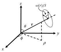
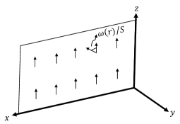
Figure 1: Schematic figure on left representing the action of the spin rotation operator for a maximally symmetric skyrmion while on right the rotation is around $y$-axis in $xz$-plane with initial spin along $z$-axis.

Rotations in the xz-plane: We consider rotations in $xz$-plane with axis of rotation being the $x$-axis, we choose the initial orientation along z-direction and hence use the eigenvector of $S_{z}$, namely, $\zeta_{z}$, for the operation. The average spin components are given by

$$\left(<S_{x}>,<S_{y}>,<S_{z}>\right)=$$

$$\left(0,-\dfrac{\sin[2\omega(\rho)]}{2},\dfrac{\cos[2\omega(\rho)]}{2}\right).$$ (12)

The spinor takes the form

$$\zeta(\textbf{r})=\begin{pmatrix}\cos[\omega(\rho)]\\ -i\sin[\omega(\rho)]\end{pmatrix}.$$ (13)

This corresponds to spin rotations out of the plane, i.e., around an axis parallel to the plane.
Considering rotations around the $y$-axis, the average spin components become

$$\left(<S_{x}>,<S_{y}>,<S_{z}>\right)=$$

$$\left(\dfrac{\sin[2\omega(\rho)]}{2},0,\dfrac{\cos[2\omega(\rho)]}{2}\right),$$ (14)

and the spinor becomes

$$\zeta(\textbf{r})=\begin{pmatrix}\cos[\omega(\rho)]\\ \sin[\omega(\rho)]\end{pmatrix}.$$ (15)

This spin texture corresponds to spin rotations within the plane, i.e., around an axis perpendicular to the plane.
Considering the rotations around $z$-axis, we get

$$\zeta(\textbf{r})=\begin{pmatrix}\cos[\omega(\rho)]-i\sin[\omega(\rho)]\\ 0\end{pmatrix},$$ (16)

and the average spin components are

$$\left(<S_{x}>,<S_{y}>,<S_{z}>\right)=(0,0,1/2),$$ (17)

which is trivial case because it corresponds to spin rotations around the same axis along which the spins are aligned, and thus will be ignored.
The spinor and the average spin components for all the possible cases of rotations around fixed axes in $xz$-plane are listed in Table 1. Considering other planes leads basically to only these two spin textures.

Rotations in $xz$-plane around fixed axes
Axis of rotation	Initial Spin Orientation	$\zeta(\textbf{r})$	$\left(<S_{x}>,<S_{y}>,<S_{z}>\right)$
$~{}~{}~{}~{}x$-axis $\begin{array}[]{l}~{}~{}~{}\theta=\pi/2,\\ ~{}~{}~{}\phi=0\end{array}$	$\zeta_{x}$	$\left(e^{-i\omega(\rho)}~{}\zeta_{x}\right)$	$\left(\frac{1}{2},0,0\right)$
	$\zeta_{y}$	$\begin{pmatrix}\dfrac{\cos[\omega(\rho)]+\sin[\omega(\rho)]}{\sqrt{2}}\\ \dfrac{i(\cos[\omega(\rho)]-\sin[\omega(\rho)])}{\sqrt{2}}\end{pmatrix}$	$\left(0,\dfrac{\cos[2\omega(\rho)]}{2},\dfrac{\sin[2\omega(\rho)]}{2}\right)$
	$\zeta_{z}$	$\begin{pmatrix}\cos[\omega(\rho)]\\ -i\sin[\omega(\rho)]\end{pmatrix}$	$\left(0,-\dfrac{\sin[2\omega(\rho)]}{2},\dfrac{\cos[2\omega(\rho)]}{2}\right)$
$~{}~{}~{}~{}y$-axis $\begin{array}[]{l}~{}~{}~{}\theta=\pi/2,\\ ~{}~{}~{}\phi=\pi/2\end{array}$	$\zeta_{x}$	$\begin{pmatrix}\dfrac{\cos[\omega(\rho)]-\sin[\omega(\rho)]}{\sqrt{2}}\\ \dfrac{\cos[\omega(\rho)]+\sin[\omega(\rho)]}{\sqrt{2}}\end{pmatrix}$	$\left(\dfrac{\cos[2\omega(\rho)]}{2},0,-\dfrac{\sin[2\omega(\rho)]}{2}\right)$
	$\zeta_{y}$	$\left(e^{-i\omega(\rho)}~{}\zeta_{y}\right)$	$\left(0,\frac{1}{2},0\right)$
	$\zeta_{z}$	$\begin{pmatrix}\cos[\omega(\rho)]\\ \sin[\omega(\rho)]\end{pmatrix}$	$\left(\dfrac{\sin[2\omega(\rho)]}{2},0,\dfrac{\cos[2\omega(\rho)]}{2}\right)$
$~{}~{}~{}~{}z$-axis $\begin{array}[]{l}~{}~{}~{}\theta=0,\\ ~{}~{}~{}\phi=\pi/2\end{array}$	$\zeta_{x}$	$\begin{pmatrix}\dfrac{\cos[\omega(\rho)]-i\sin[\omega(\rho)]}{\sqrt{2}}\\ \dfrac{\cos[\omega(\rho)]+i\sin[\omega(\rho)]}{\sqrt{2}}\end{pmatrix}$	$\left(\dfrac{\cos[2\omega(\rho)]}{2},\dfrac{\sin[2\omega(\rho)]}{2},0\right)$
	$\zeta_{y}$	$\begin{pmatrix}\dfrac{\cos[\omega(\rho)]-i\sin[\omega(\rho)]}{\sqrt{2}}\\ \dfrac{i\cos[\omega(\rho)]-\sin[\omega(\rho)]}{\sqrt{2}}\end{pmatrix}$	$\left(-\dfrac{\sin[2\omega(\rho)]}{2},\dfrac{\cos[2\omega(\rho)]}{2},0\right)$
	$\zeta_{z}$	$\left(e^{-i\omega(\rho)}~{}\zeta_{z}\right)$	$\left(0,0,\frac{1}{2}\right)$

Table 1: All possible cases of rotations in the $xz$-plane around three possible fixed axes of rotation, $x$-, $y$-, and $z$-axis, with three possible initial spin directions, $\zeta_{x}$, $\zeta_{y}$, $\zeta_{z}$. The spinor wavefunction, $\zeta({\bf r})$, and the average spin components, $<S_{x}>$, $<S_{y}>$ and $<S_{z}>$, are calculated using Eqs. (II, 9,10,11).

Rotations in the xy-plane around $\bf{\rho}$ : We consider the rotations around $\rho=\sqrt{x^{2}+y^{2}}$. Since the axis of rotation changes with $\phi$, the spinor components and the texture demand also on $\phi$, as listed in Table II.

Rotations in $xy$-plane around $\rho$
Axis of rotation	Initial spin	$\zeta(\textbf{r})$	$\left(<S_{x}>,<S_{y}>,<S_{z}>\right)$
$\rho=~{}\sqrt{x^{2}+y^{2}}$ $~{}~{}(\theta=\pi/2)$	$\zeta_{x}$	$\begin{pmatrix}\dfrac{\cos[\omega(\rho)]-ie^{-i\phi}\sin[\omega(\rho)]}{\sqrt{2}}\\ \dfrac{\cos[\omega(\rho)]-ie^{i\phi}\sin[\omega(\rho)]}{\sqrt{2}}\end{pmatrix}$	$\left(\dfrac{\cos^{2}[\omega(\rho)]+\cos(2\phi)\sin^{2}[\omega(\rho)]}{2},\dfrac{\sin(2\phi)\sin^{2}[\omega(\rho)]}{2},-\dfrac{\sin(\phi)\sin[2\omega(\rho)]}{2}\right)$
	$\zeta_{y}$	$\begin{pmatrix}\dfrac{\cos[\omega(\rho)]+e^{-i\phi}\sin[\omega(\rho)]}{\sqrt{2}}\\ \dfrac{i(\cos[\omega(\rho)]-e^{i\phi}\sin[\omega(\rho)])}{\sqrt{2}}\end{pmatrix}$	$\left(\dfrac{\sin(2\phi)\sin^{2}[\omega(\rho)]}{2},\dfrac{\cos^{2}[\omega(\rho)]-\cos(2\phi)\sin^{2}[\omega(\rho)]}{2},\dfrac{\cos(\phi)\sin[2\omega(\rho)]}{2}\right)$
	$\zeta_{z}$	$\begin{pmatrix}\cos[\omega(\rho)]\\ e^{-i(\frac{\pi}{2}-\phi)}\sin[\omega(\rho)]\end{pmatrix}$	$\left(\dfrac{\sin(\phi)\sin[2\omega(\rho)]}{2},-\dfrac{\cos(\phi)\sin[2\omega(\rho)]}{2},\dfrac{\cos[2\omega(\rho)]}{2}\right)$

Table 2: All possible cases of rotations in the $xy$-plane around $\rho$ with three possible initial spin directions, $\zeta_{x}$, $\zeta_{y}$, $\zeta_{z}$. The spinor wavefunction, $\zeta({\bf r})$, and the average spin components, $<S_{x}>$, $<S_{y}>$ and $<S_{z}>$, are calculated using Eqs. (II, 9,10,11).

III Mapping the spin-1/2 system to a 2D Manakov system

We have shown in the previous section that the spinor wavefunction of a skyrmion can be written in a specific form that corresponds to spin rotations. There are many such specific forms depending on the plane at which the spins are located in, the axis of spin rotations, and the initial spin orientation, as summarized by Tables 1 and 2. This procedure is effectively a change of variables amounting to a change in the representation from the spinor components, $\psi_{1}$ and $\psi_{2}$, to the total density $n$ and angle of rotation $\omega/S$. Considering one of these specific cases, namely spinors restricted to the $xz$-plane with spin rotations around the $y$-axis as shown schematically in Fig. 1b, the spinor becomes

$$\begin{pmatrix}\psi_{1}(\rho,\phi,t)\\ \psi_{2}(\rho,\phi,t)\end{pmatrix}=\sqrt{n(\rho,t)}\begin{pmatrix}e^{il_{1}\phi}\cos[\omega(\rho)]\\ e^{il_{2}\phi}\sin[\omega(\rho)]\end{pmatrix},$$ (18)

where $\rho=\sqrt{x^{2}+z^{2}}$ and $\phi$ is the angle between $\rho$ and the $z$-axis. We have added the phase operator $e^{il\phi}$ to allow for non-zero angular momentum of any of the two components. This accounts for an acquired phase while spins are rotated. This spin-1/2 system is then mapped to a 2D Manakov system obtained by substituting the spinor (18) in the NLSE, (2),

$$i\begin{pmatrix}\psi_{1}(\rho,\phi,t)\\ \psi_{2}(\rho,\phi,t)\end{pmatrix}_{t} = -\begin{pmatrix}\psi_{1}(\rho,\phi,t)\\ \psi_{2}(\rho,\phi,t)\end{pmatrix}_{\rho\rho}$$ (19)

$$- \frac{1}{\rho}\begin{pmatrix}\psi_{1}(\rho,\phi,t)\\ \psi_{2}(\rho,\phi,t)\end{pmatrix}_{\rho}$$

$$- \frac{1}{\rho^{2}}\begin{pmatrix}\psi_{1}(\rho,\phi,t)\\ \psi_{2}(\rho,\phi,t)\end{pmatrix}_{\phi\phi}$$

$$- \gamma(|\psi_{1}(\rho,\phi,t)|^{2}+|\psi_{2}(\rho,\phi,t)|^{2})$$

$$\times \begin{pmatrix}\psi_{1}(\rho,\phi,t)\\ \psi_{2}(\rho,\phi,t)\end{pmatrix}.$$

The problem then reduces to solving this system, which we describe in the next section. The solutions $\psi_{1}(\rho,\phi,t)$ and $\psi_{2}(\rho,\phi,t)$ can then be used in (18) to obtain two coupled equations for $n(\rho,t)$ and $\omega(\rho)$. Solving these equations gives the texture of the skyrmion through $<S_{x}>$, $<S_{y}>$, and $<S_{z}>$, as well as its density profile, $n(\rho,t)$.

IV Solving the Manakov system

We present different methods of solving the Manakov system (19) in order to generate the non-trivial spin texture. All methods mentioned below are well known and powerful techniques in analytical and numerical analysis but our desired results are achieved by the numerical technique described in Sec. IV.3. The other methods paved the way for developing the numerical technique on a trial function, so we include them in this section. At first, we attempt to map the 2D Manakov system (19) into the 1D Manakov system which is integrable with many known solutions. While this leads to nontrivial skyrmion textures, the corresponding spinor densities diverge at $\rho=0$. As an alternative approach we employ a power series method to find well-behaved spinor densities. However, the associated skyrmion texture turns out to be trivial for such a case. Finally, well-behaved spinor densities with nontrivial skyrmion textures are obtained by employing a trial function that takes into account the spin texture of a specific case of rotation as detailed in Tables 1 and II, and then solving numerically the NLSE for $n(\rho,t)$ and $\omega(\rho)$.

IV.1 Similarity transformation

At first, we transform the 2D Manakov system into the fundamental 1D Manakov system via a simple similarity transformation. This will enable us then to find the new solutions of 2D Manakov system by using all known solutions of the fundamental 1D Manakov system. We start with the simplest case for the solution of 2D Manakov system, namely, the cylindrically symmetric solution. As there is no $\phi$ dependence in this case, corresponding to $l_{1}=l_{2}=0$, we are left with

$$i\begin{pmatrix}\psi_{1}(\rho,t)\\ \psi_{2}(\rho,t)\end{pmatrix}_{t}=-\begin{pmatrix}\psi_{1}(\rho,t)\\ \psi_{2}(\rho,t)\end{pmatrix}_{\rho\rho}-\frac{1}{\rho}\begin{pmatrix}\psi_{1}(\rho,t)\\ \psi_{2}(\rho,t)\end{pmatrix}_{\rho}$$

$$-\gamma(|\psi_{1}(\rho,t)|^{2}+|\psi_{2}(\rho,t)|^{2})\begin{pmatrix}\psi_{1}(\rho,t)\\ \psi_{2}(\rho,t)\end{pmatrix}.$$ (20)

To reduce this system into the integrable 1D Manakov system we apply the following simple transformation

$$\psi_{1,2}=\rho^{n}~{}\Phi_{1,2}$$ (21)

to the above 2D Manakov system (IV.1). The system then reduces to the fundamental 1D Manakov system for $n=-1/2$

$$\psi_{1,2}=\dfrac{1}{\sqrt{\rho}}~{}\Phi_{1,2}.$$ (22)

For all solutions of the 1D Manakov system, $\Phi_{1,2}$, that are finite at $\rho=0$, the solutions of the 2D Manakov system $\psi_{1,2}$ diverge at $\rho=0$. This applies to all known solutions of the 1D Manakov system which we have used in Appendix A, except the solution $(\Phi_{1},\Phi_{2})\sim(\tanh(\rho),\operatorname{sech}(\rho))$. The $\tanh(\rho)$ part of this particular solution is zero at $\rho=0$, and thus $\psi_{1}\sim\Phi_{1}/\sqrt{\rho}$ does not diverge at $\rho=0$. However, the other component $\psi_{2}\sim\operatorname{sech}(\rho)/\sqrt{\rho}$ diverges at $\rho=0$. For all other solutions, both components diverge at $\rho=0$. To establish the link between the solutions of the 1D and 2D Manakov systems in a rigorous manner, we consider the following most general form of a similarity transformation

$$p_{1}~{}\Bigg{[}i~{}\psi_{1_{t}}+b_{11}\Big{[}\psi_{1_{\rho\rho}}+\frac{1}{\rho}\psi_{1_{\rho}}\Big{]}+\Big{[}b_{12}|\psi_{1}|^{2}+$$

$$b_{13}|\psi_{2}|^{2}\Big{]}\psi_{1}+\Big{[}b_{14r}+ib_{14i}\Big{]}\psi_{1}\Bigg{]}=0,$$

$$p_{2}~{}\Bigg{[}i~{}\psi_{2_{t}}+b_{21}\Big{[}\psi_{2_{\rho\rho}}+\frac{1}{\rho}\psi_{2_{\rho}}\Big{]}+\Big{[}b_{22}|\psi_{1}|^{2}+$$

$$b_{23}|\psi_{2}|^{2}\Big{]}\psi_{2}+\Big{[}b_{24r}+ib_{24i}\Big{]}\psi_{2}\Bigg{]}=0,$$ (23)

where $p_{1}$, $p_{2}$, $b_{11}$, $b_{21}$, $b_{12}$, $b_{22}$, $b_{13}$, $b_{23}$, $b_{14r}$, $b_{24r}$, $b_{14i}$, and $b_{24i}$ are all functions of $(\rho,t)$, and are arbitrary real coefficients. We apply the following transformation on the system (IV.1)

$$\Psi_{1}(\vec{r},t)=A(\rho,t)~{}e^{iB_{1}(\rho,t)}~{}F[P(\rho,t),T(\rho,t)],$$

$$\Psi_{2}(\vec{r},t)=A(\rho,t)~{}e^{iB_{2}(\rho,t)}~{}G[P(\rho,t),T(\rho,t)].$$ (24)

Here, $A(\rho,t)$, $B_{1}(\rho,t)$, $B_{2}(\rho,t)$, $P(\rho,t)$, and $T(\rho,t)$ are all defined as real functions. Substituting (IV.1) in (IV.1) and requiring the resulting equations to take the form of the following fundamental Manakov system

$$iF_{t}(P,T)+a_{11}F_{\rho\rho}(P,T)+\Big{[}a_{12}|F(P,T)|^{2}+$$

$$a_{13}|G(P,T)|^{2}\Big{]}F(P,T)=0,$$

$$iG_{t}(P,T)+a_{21}G_{\rho\rho}(P,T)+\Big{[}a_{22}|F(P,T)|^{2}+$$

$$a_{23}|G(P,T)|^{2}\Big{]}G(P,T)=0,$$ (25)

gives a set of equations for the unknown functions. Solutions of these equations are relegated to Appendix B. We listed few solutions for the 2D Manakov system obtained using this approach in Appendix A. Here again, we end up with the solutions having divergences at $\rho=0$ and therefore they will be discarded for no physical significance. Seeking solutions which are well-behaved at $\rho=0$, we employ in the next section an Iterative Power Series (IPS) method [21].

IV.2 Power series method

We apply the IPS method with a stationary solution given by

$$\psi_{1}(\rho,t)=Z_{1}(\rho)\,e^{i\,\alpha_{1}\,t},$$

$$\psi_{2}(\rho,t)=Z_{2}(\rho)\,e^{i\,\alpha_{2}\,t},$$ (26)

where $Z_{1}(\rho)$ and $Z_{2}(\rho)$ are real functions and $\alpha_{1}$ and $\alpha_{2}$ are arbitrary real constants. Using this solution, Eq. (IV.1) renders to the following ordinary differential equations

$$\frac{1}{\rho}\,Z_{1}^{\prime}(\rho)+Z_{1}^{\prime\prime}(\rho)+Z_{1}(\rho)\left[\gamma\,Z_{2}^{2}(\rho)-\alpha_{1}\right]$$

$$+\gamma\,Z_{1}^{3}(\rho)=0,$$

$$\frac{1}{\rho}\,Z_{2}^{\prime}(\rho)+Z_{2}^{\prime\prime}(\rho)+Z_{2}(\rho)\left[\gamma\,Z_{1}^{2}(\rho)-\alpha_{2}\right]$$

$$+\gamma\,Z_{2}^{3}(\rho)=0.$$ (27)

In the following, we give a brief algorithm description of the IPS method for obtaining a convergent power series solution to (IV.2):

1. Expand $Z_{1}(\rho)$ and $Z_{2}(\rho)$ in power series around an arbitrary real initial point $\rho_{0}$

$Z_{1}(\rho)=a_{0}+a_{1}\,(\rho-\rho_{0})+\sum_{n=2}^{n_{max}}a_{n}(\rho-\rho_{0})^{n}$, $Z_{2}(\rho)=b_{0}+b_{1}\,(\rho-\rho_{0})+\sum_{n=2}^{n_{max}}b_{n}(\rho-\rho_{0})^{n}$. 2. Set initial values $\{a_{0},a_{1}\}$ and $\{b_{0},b_{1}\}$ for $Z_{1}(\rho)$ and $Z_{2}(\rho)$, respectively. 3. Substitute in (IV.2) to obtain the recursion relation for $a_{n}$ and $b_{n}$ in terms of $a_{0}$, $a_{1}$, $b_{0}$, and $b_{1}$. 4. Calculate $Z_{1}(\Delta)$, ${Z_{1}}^{\prime}(\Delta)$, $Z_{2}(\Delta)$, and ${Z_{2}}^{\prime}(\Delta)$, where $\Delta=(\rho-\rho_{0})/I$ and $I$ is an integer larger than 1. 5. Assign: $a_{0}=Z_{1}(\Delta)$, $a_{1}={Z_{1}}^{\prime}(\Delta)$, $b_{0}=Z_{2}(\Delta)$, and $b_{1}={Z_{2}}^{\prime}(\Delta)$. 6. Obtain $a_{n}$ and $b_{n}$ in terms of $a_{0}$, $a_{1}$, $b_{0}$, and $b_{1}$. 7. Repeat steps 2-6 $I$ times. 8. At the $I$th step, $a_{0}$ will correspond to the power series of $Z_{1}(\rho)$ and $b_{0}$ will correspond to the power series of $Z_{2}(\rho)$.

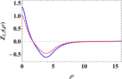
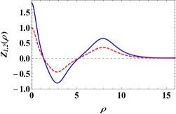
Figure 2: (Color online) Stationary power series solutions of (IV.2) with different number of nodes. Dashed (red) is $Z_{1}(\rho)$ and solid (blue) is $Z_{2}(\rho)$. The left subfigure is single-node solution with $a_{0}=1.3293391$, root at $r=1.85$ and the right subfigure is double-node solution with $a_{0}=1.8079999$, roots at $r=1.58,5.45$. Parameters used are: $b_{0}=1$, $a_{1}=b_{1}=0$, $\alpha_{1}=\alpha_{2}=0.5$, $\gamma=2$, $n_{max}=2$, $I=5000$, and $\Delta=0.0032$. Employing the algorithm above, we obtain a family of infinite number of convergent solutions by tuning the parameter $a_{0}$ and fixing the other parameters. In Fig. 2, we present two plots showing the single-node and double-node solutions obtained with $I=5000$ and $n_{max}=2$. Although this method provides an infinite number of non-divergent densities, due to the scalar symmetry between $\psi_{1}(\rho,t)$ and $\psi_{2}(\rho,t)$, the spin textures corresponding to these solutions which is proportional to $\psi_{2}/\psi_{1}$, turn out to be trivial.

IV.3 Numerical solutions

Here, we introduce a new procedure that leads to nondiverging and nontrivial spin textures. We start with a trial function which is constructed on the basis of the spinor wave function for rotation cases listed in Tables 1 and II. For instance, we consider a case of rotation from Table 1 in $xz$-plane with initial spin along $z$-axis and $y$-axis is the axis of rotation. Our ansatz, for this case becomes:

$$\psi_{1}(\rho,t)=a(\rho)\cos[\omega(\rho)],$$

$$\psi_{2}(\rho,t)=a(\rho)\sin[\omega(\rho)],$$ (28)

where $a(\rho)=\sqrt{n(\rho)}$. Substituting this trial function into the system given in Eq. (IV.1) and then requesting the coefficients of $\cos[\omega(\rho)]$ and $\sin[\omega(\rho)]$ to vanish separately, we get two coupled equations in terms of $a(\rho)$ and $\omega(\rho)$

$$2a^{\prime}(\rho)\omega^{\prime}(\rho)+a(\rho)\Big{(}\dfrac{\omega^{\prime}(\rho)}{\rho}+\omega^{\prime\prime}(\rho)\Big{)}=0,$$ (29)

$$\gamma~{}a^{3}(\rho)+\dfrac{a^{\prime}(\rho)}{\rho}-a(\rho)\Big{(}\dfrac{1}{4\rho^{2}}+\omega^{\prime 2}(\rho)\Big{)}+ra^{\prime}(\rho)=0.$$ (30)

We solve Eq. (29) for $\omega(\rho)$ as

$$\omega(\rho)=\int\dfrac{c_{1}}{\rho~{}a(\rho)^{2}}d\rho+c_{2},$$ (31)

where $c_{1}$ and $c_{2}$ are constants of integration. By substituting the above relation for $\omega(\rho)$ in Eq. (30), our problem (IV.1) is reduced into the following single equation

$$c_{1}^{2}-\gamma~{}\rho^{2}~{}a^{6}-\rho~{}a^{3}\Big{(}a^{\prime}+\rho~{}a^{\prime\prime}\Big{)}=0.$$ (32)

We solve this equation for $a(\rho)$ numerically. The initial conditions used are $a(0)=a_{0}$ and $a^{\prime}(0)=0$. We choose $a_{0}$ as the tuning parameter for the calculation. The results are shown in Fig. 3.

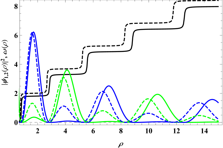
Figure 3: (Color online) The numerical solutions of the spinor components given by Eq. (IV.3) of the system (29) and (30). The solutions correspond to alternating spin-up (green) and spin-down (blue) components of the spinor wave function. The black curve corresponds to $\omega(\rho)$. The solid and dashed curves correspond to the circle and square in Fig 10, which represent a stable and a metastable skyrmion, respectively. Parameters used are: $\gamma=c_{1}=1/2$, and $a_{0}=2.9$.

Similarly, any of the rotation cases given in Tables 1 and II can be considered for the substitution of $\psi_{1}(\rho,t)$ and $\psi_{2}(\rho,t)$. It turns out, however, that all cases of rotations lead to the same Eq. (32) with the same relation of $\omega(\rho)$ as given in Eq. (31). All possible cases of rotations discussed in Table 1 correspond to the two fundamental types of skyrmions which represent rotation either in-plane or out-of-plane. The rotation of spin around its own axis is a trivial case. The in-plane and out-of-plane spin textures $<S_{x}>$ and $<S_{z}>$ given by the expressions in Table 1 for the cases of rotation around $y$-axis and $x$-axis, respectively, with initial spin along $z$-axis are shown in Fig. 4. These results are obtained from solving the Eq. (32) numerically. The structure of $<S_{y}>$ is trivial (constant/plain texture) for this case. These spin textures are, however, modulated by the total density of both spin components. This kind of modulation is applicable for the adjustment of carrier distributions for current density change and light intensity [24] and also for the nonlinear resonator [25]. To show such modulations, we plot in Fig. 5 the quantities $n\,<S_{x}>$ and $n\,<S_{z}>$ for the case of in-plane rotations.

Figure 4: In-plane and out-of-plane vector representations of skyrmions in spin-1/2 system for the case of rotation in $xz$-plane around $y$-axis and $x$-axis, respectively with initial spin along $z$-axis. Parameters used are the same as in Fig. 3.

In order to find the spin texture of skyrmions for the cases of rotations around $\rho$ in the $xy$-plane, as listed in Table II, we follow the same procedure as discussed above. However, for the case of rotation around $\rho$, the spin texture will be dependent not only on the rotation angle $\omega(\rho)$ but also on the projection angle $\phi$, as a result we expect fundamentally different skyrmions. We consider the system (19) to be solved for this case which includes also $\phi$ dependence.

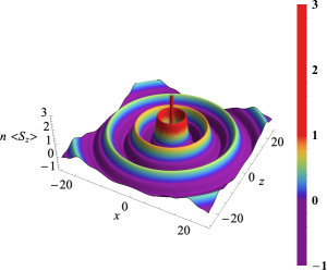
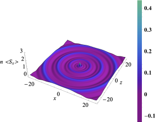
Figure 5: False-colour figures representing the average spin texture modulated by the total density, namely $n\,<S_{z}>$ and $n\,<S_{x}>$ for a skyrmion in a spin-1/2 system in $xz$-plane with initial spin along $z$-axis which is given in Table 1. The axis of rotation is $y$-axis. Parameters used are the same as in Fig. 3.

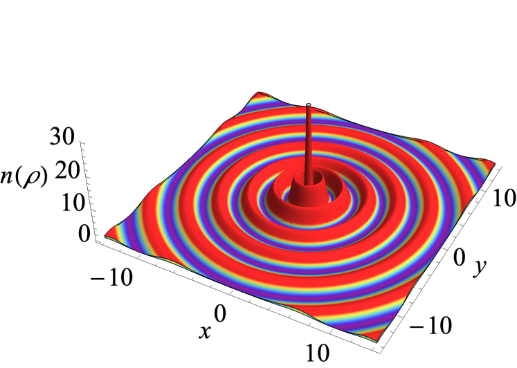
Figure 6: The total density for the case of rotation around $\rho$ in $xy$-plane with initial spin along $z$-axis.

Now, we take an example from Table II of the rotation around $\rho$ in $xy$-plane with initial spin oriented along $z$-axis and the trial function becomes

$$\psi_{1}(\rho,\phi,t) = a(\rho)~{}e^{ik_{1}\phi}\cos[\omega(\rho)],$$

$$\psi_{2}(\rho,\phi,t) = a(\rho)~{}e^{ik_{2}\phi}\sin[\omega(\rho)]\times$$ (33)

$$e^{-i(\pi/2-\phi)},$$

where $k_{1}$ and $k_{2}$ are related as $k_{1}=1+k_{2}$. The total spinor densities for this case are shown in Fig. 6. It is also noteworthy that all cases of rotation around $\rho$ lead to the same equation, (32). The spin texture for the case of rotation in $xy$-plane around $\rho$ with initial spin along $z$-axis is given in Fig. 7. It can be seen from the figure, that the $<S_{z}>$ component has the same structure as in the previous case shown in Fig. 4 because there is no $\phi$ dependence in this component. The vector representation of the skyrmions in spin-1/2 system for the above mentioned rotation is shown below in Fig. 9. We found two other unique skyrmion textures for the case of rotation around $\rho$ which are shown in Fig. 8. The orientation of initial spin is along $y$-axis and the expressions for average spin components are given in Table II. It is clear from the expressions of average spin components given in Table II that there are four distinguished textures for the case of rotation around $\rho$, as shown in Figs. 7 and 8. For the case of axial symmetry as discussed in Table 1, we have only two fundamental skyrmion textures which are plotted in Fig. 4.

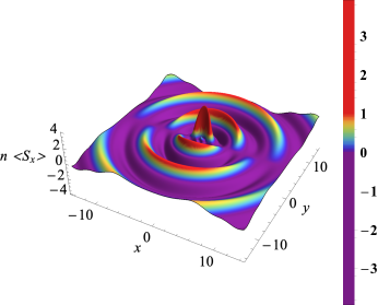
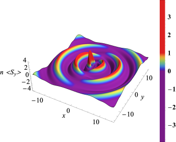
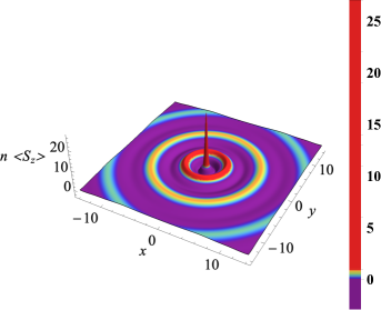
Figure 7: False-colour figures representing the average spin $n\,<S_{x}>$, $n\,<S_{y}>$, and $n\,<S_{z}>$ for a skyrmion in a spin-1/2 system with the rotation around $\rho$ in $xy$-plane. The initial spin orientation is along $z$-axis.

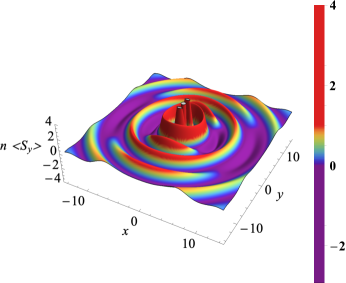
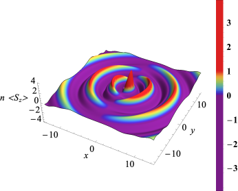
Figure 8: False-colour figures representing the average spin $n\,<S_{x}>$, $n\,<S_{y}>$, and $n\,<S_{z}>$ for a skyrmion in a spin-1/2 system with the rotation around $\rho$ in $xy$-plane. The initial spin orientation is along $y$-axis.

Figure 9: The vector representation of skyrmions in spin-1/2 system for the case of rotation around $\rho$ in $xy$-plane with initial spin along $z$-axis.

V Stability of the non-trivial Skyrmions

In order to investigate the stability of the skyrmions, we calculated the energy functional for both cases i.e rotation around fixed axes (axial symmetry) as given in Table 1 and rotations around $\rho$ which is summarized in Table II. The energy functional corresponding to system (19) reads

$$E = \int_{0}^{2\pi}d\phi\int_{0}^{\infty}\Big{[}\alpha\Big{(}|\Psi_{1}|^{2}+|\Psi_{2}|^{2}\Big{)}$$ (34)

$$- \dfrac{\gamma}{2}\Big{(}|\Psi_{1}|^{2}+|\Psi_{2}|^{2}+2|\Psi_{1}|^{2}|\Psi_{2}|^{2}\Big{)}+|\Psi_{1\rho}|^{2}$$

$$+ |\Psi_{2\rho}|^{2}+\dfrac{1}{\rho^{2}}\Big{(}|\Psi_{1\phi}|^{2}+|\Psi_{2\phi}|^{2}\Big{)}\Big{]}\rho~{}d\rho.$$

We substitute the specific trial function in Eq. (34) to find the expression for the energy functional of that specific case of rotation. For instance, we substitute the trial function (IV.3) for the case of rotation around $\rho$ in $xy$-plane with initial spin along $z$-axis in above relation and find the following expression

$$E = \int\Big{[}-\dfrac{1}{2}\gamma~{}a(\rho)^{4}+a^{\prime}(\rho)^{2}+\dfrac{c_{1}^{4}}{\rho^{2}~{}a(\rho)^{2}}+$$ (35)

$$\alpha~{}a(\rho)^{2}+\dfrac{a(\rho)^{2}(1+2k_{2}+k_{2}^{2})}{\rho^{2}}\Big{]}\rho~{}d\rho,$$

where $k_{1}=1+k_{2}$. While considering axial symmetry (IV.1), for example, rotation around $y$-axis with initial spin along $z$-axis, we use the trial function (IV.3) into (34) and obtain the following result for energy functional

$$E = \int\Big{[}-\dfrac{1}{2}~{}\gamma~{}a(\rho)^{4}+a^{\prime}(\rho)^{2}+\alpha~{}a(\rho)^{2}$$ (36)

$$+ \dfrac{c_{1}^{4}}{\rho^{2}~{}a(\rho)^{2}}\Big{]}\rho~{}d\rho.$$

We find a global minimum in the energy functional as well as many local minima. The local minima correspond to a state of concentric rings with spins alternating sharply between 1/2 and -1/2. The total density within a ring is contributed by only one component of spin, either spin up or spin down. On the other hand, mixed states of spin in which the total density is contributed by both component of spin, i.e spin up and spin down correspond to a metastable skyrmion. The profile of the two spin componenets corresponding to a stable and a metastable skyrmion (circle and square on the energy curve) are shown in Fig. 3.

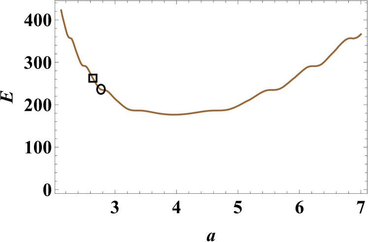
Figure 10: The energy for the case of rotation around $y$-axis with initial spin along $z$-axis.

VI Conclusion

We mapped the spin-1/2 system to a 2D Manakov system through a rotation operator that gives the spin texture of skyrmions. We have investigated all possible 2D skyrmion textures, as listed in Tables 1 and 2. We solved the 2D Manakov system using various analytical and numerical methods. While the similarity transformation method maps all solutions of the integrable 1D Manakov system to the 2D Manakov system, the solutions of the latter turn out to diverge at $\rho=0$. Nondiverging solutions were then obtained using a power series method. However, the spin texture associated with these solutions turned out to be trivial, i.e., no texture. Finally, we considered a numerical solution of a system of coupled equations for the skyrmion density, $n(\rho,\phi)$, and texture, $\omega(\rho,\phi)$. This led to nondiverging and nontrivial spin textures. Then, we investigated the stability of these nontrivial nondiverging skyrmions by calculating their energy functional in terms of their effective size. It turned out that stable skyrmions correspond to concentric rings of spin components alternating between spin up and spin down. Metastable states, where energy is either increasing or decreasing with skyrmion size, correspond to concentric rings of mixed spin components. Our results show that, in contrast with the established fact that in two dimensions localized solutions of the NLSE are unstable, the two spin states stabilize each other against collapse and allow for nontrivial stable two-dimensional topological excitations. Our results are also applicable to doubly polarized optical pulses. We strongly believe that this work is an important addition to the effort of realizing topological excitations.

Appendix A Solutions of the 2D Manakov system

Using the similarity transformation described in Sec. IV.1, we found many new solutions for the 2D Manakov system (19), here we mentioned only two of them for their significance. The full list of solution is compiled by Ref. [26]. Solution-1

$$\psi_{1}(\rho,t)=\frac{1}{\sqrt{\rho}}{\tanh\left(\sqrt{\dfrac{3}{8}}~{}\rho\right)}~{}e^{-i(1-3t)}$$ (A.1)

$$\psi_{2}(\rho,t)=\sqrt{\frac{5}{2}}\frac{1}{\sqrt{\rho}}{\operatorname{sech}\left(\sqrt{\dfrac{3}{8}}~{}\rho\right)}~{}e^{\frac{15}{8}i(-1+t)}$$ (A.2)

The choice of parameters are $a_{11}=-1$, $a_{12}=2$, $a_{21}=1$, and $a_{13}=a_{22}=a_{23}=\frac{1}{2}$. See Fig. A.1.

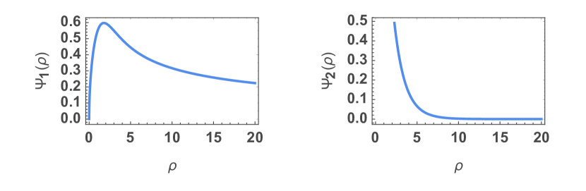
Figure A.1: The graphical representation of $\psi_{1}(\rho)$ and $\psi_{2}(\rho)$ for solution-1.

Solution-2

$$\psi_{1}(\rho,t)=\frac{1}{3\sqrt{\rho}}\Big{(}-2+3\operatorname{sech}^{2}[\rho]\Big{)}~{}e^{2i(1-t)}$$ (A.3)

$$\psi_{2}(\rho,t)=\frac{1}{\sqrt{\rho}}~{}{\operatorname{sech}^{2}[\rho]}~{}e^{-2i(1-t)}$$ (A.4)

The parameters are $a_{11}=a_{21}=1$, $a_{12}=a_{22}=-\frac{9}{2}$, and $a_{13}=a_{23}=\frac{9}{2}$. See Fig. A.2.

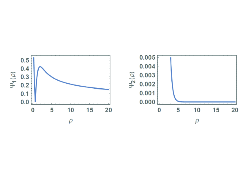
Figure A.2: The graphical representation of $\psi_{1}(\rho)$ and $\psi_{2}(\rho)$ for solution-2.

Appendix B Similarity transformation

The results of all the unknown quantities in (IV.1) and all the coefficients in (IV.1) are listed below: For $\bf{\Psi_{1}(\vec{r},t)}$: $T(\rho,t)=g_{1}(t)$ p1(ρ,t)=1eiB1(ρ,t)A(ρ,t)g1′(t), b11(ρ,t)=a11g1′(t)P2ρ(ρ,t), b12(ρ,t)=a12g1′(t)A2(ρ,t), b13(ρ,t)=a13g1′(t)A2(ρ,t), A(ρ,t)=g2(t)ρPρ(ρ,t), B1(ρ,t)=-∫Pt(ρ,t)Pρ(ρ,t)2a11g1′(t)dρ+g3(t), b14i(ρ,t)=-g2′(t)g2(t)