Energy spectra of graphene quantum dots induced between Landau levels

Abstract

When an energy gap is induced in monolayer graphene the valley degeneracy is broken and the energy spectrum of a confined system such as a quantum dot, becomes rather complex exhibiting many irregular level crossings and small energy spacings which are very sensitive to the applied magnetic field. Here we study the energy spectrum of a graphene quantum dot that is formed between Landau levels, and show that for the appropriate potential well the dot energy spectrum in the first Landau gap can have a simple pattern with energies coming from one of the two valleys only. This part of the spectrum has no crossings, has specific angular momentum numbers, and the energy spacing can be large enough, consequently, it can be probed with standard spectroscopic techniques. The magnetic field dependence of the dot levels as well as the effect of the mass-induced energy gap are examined, and some regimes leading to a controllable quantum dot are specified. At high magnetic fields and negative angular momentum a simple approximate method to the Dirac equation is developed which gives further insight into the physics. The approximate energies exhibit the correct trends and agree well with the exact energies.

I Introduction

Some experiments freitag16 ; freitag18 ; li ; lee have shown that a quantum dot can be formed in a single sheet of graphene by adjusting the tip-induced potential of a scanning tunnelling microscope (STM). In a uniform magnetic field discrete energy levels have been probed between bulk Landau levels, freitag16 ; freitag18 and the electronic properties of confined states have been explored. freitag16 ; freitag18 ; li ; lee ; qiao To better control the tunability of the quantum devices in the experimental studies an energy gap is usually induced at the Dirac points $K$ and $K^{\prime}$ of the band structure. Without the energy gap the two valleys at the Dirac points are degenerate and the charge carriers are massless. rozhkov Inducing an energy gap between the conduction and the valence bands leads to charge carriers with mass and the valley degeneracy is broken.

In a graphene sheet the energy gap can be induced with some simple techniques balog ; wang ; zhou ; fan ; shemella however, breaking the valley degeneracy leads to more complex energy spectra for a confined graphene system, since the energies of the charge carriers depend on the specific valley. The resulting energy spectra exhibit many level crossings as well as anti-crossings, and small energy spacings which are rather sensitive to the applied magnetic field. These features could make difficult the use of graphene dots to opto-electronics and valleytronics applications. schaibley ; karanikolas

In the present work we study the energy spectrum of a graphene quantum dot that is formed between bulk Landau levels, and show that for the appropriate fields the dot energy spectrum can have a simple pattern. Specifically, if we focus on the first Landau gap, namely, between the Landau levels $-1$ and $0$, then there is an energy range with discrete energies coming from one of the two valleys only. Thus, a graphene dot with a specific valley index can be realized. We demonstrate that the dot energy spectrum consists of specific angular momentum values and has no crossings, simplifying drastically the identification of the dot energy levels. Our calculations show that when the mass term is a few tens of meV and the applied magnetic field is a few Tesla, the typical energy spacing can be a few meV. By adjusting the STM induced potential well the discrete levels of the dot formed in the first Landau gap can be energetically isolated and lie away from the bulk Landau levels.

To obtain further insight into the physics we develop an approximate method to compute the dot energies. The method takes into account the fact that the zeroth Landau level has a Dirac state with one component zero, and even though this component becomes nonzero in the presence of the STM potential, it can still be vanishingly small compared to the second component. Using this condition we derive an approximate Schrodinger equation for the dominant component of the Dirac state. We find that at high fields and negative angular momentum the approximate energies exhibit the correct potential dependence, and are in a good agreement with the exact ones. The typical error is of the order of $1\%-2\%$, and depending on the specific parameters the error can decrease to less than $0.1\%$.

Only in the proper range of parameters the quantum dot energy spectra have a simple pattern. Anticrossing points which are relevant to the Klein tunnelling effect do not occur in the range of parameters used in this work. Quantum dots at low magnetic fields, typically lower than $0.5$ T, exhibiting Klein tunnelling have been theoretically examined earlier giavaras09 ; giavaras12 but these dots might be more difficult to probe due to the relatively small energy spacings and the fabrication of the required dot confining potential. giavaras09 Quantum dots in the Klein tunnelling regime have also more complicated quantum states and the approximate method developed in this work is inapplicable.

The quantum dot system studied here is edge-free therefore the reported results are insensitive to the microscopic details of the edges. This property offers a superior control over the dot states compared to dot states formed in nano-sheets of graphene. rozhkov The results are relevant to other confined systems formed in two-dimensional materials by external fields, moriyama ; abdullah ; caneva ; keren ; recher ; jakubsky ; sadrara ; giavaras11 ; kandemir ; maksym as well as to general hybrid graphene-based systems including defects and heterostructures. gold ; yuli ; walkup ; giorgos ; schattauer ; mirzakhani ; myli ; dnle

Section II presents the physical model of the graphene quantum dot and explains with some qualitative arguments how the discrete levels of the dot emerge from the bulk Landau levels. The energy range of interest is also specified in Sec. II, and then in Sec. III the energy spectra of the quantum dot are studied. In Sec. IV an approximate method to derive the dot energies is presented and a comparison with the exact energies is made. The conclusions are presented in Sec. V. Finally, in Appendices A, B and C the quantum dot equations are derived and some further results are presented.

II Quantum dots formed in the first Landau gap

In the continuum approximation the charge carriers in graphene satisfy the Dirac equation rozhkov

$$[v_{\text{F}}\bm{\sigma}\cdot({\bf p}+e{\bf A})+V+\tau\Delta\sigma_{z}/2]\Psi=E\Psi,$$ (1)

with $v_{\text{F}}=10^{6}$ m s^-1, ${\bf p}=(p_{x},p_{y})$ is the momentum operator, and $\bm{\sigma}=(\sigma_{x},\sigma_{y})$, $\sigma_{z}$ are the Pauli matrices. A uniform magnetic field $B$ is perpendicular to the graphene sheet in the $z$-direction and the magnetic vector potential is $A_{\theta}(r)=Br/2$ in the azimuthal direction, where $r$ is the radial coordinate. The scalar potential has the form $V(r)=-V_{0}\exp(-r^{2}/2L^{2})$ which models the STM-induced potential well with an effective depth $V_{0}\geq 0$. The effective width is controlled by the parameter $L$ which is taken to be $\sqrt{2}L=40$ nm unless otherwise specified. The mass term is denoted by $\Delta/2$ giving rise to an energy gap equal to $\Delta$, and $\tau=1$ $(-1)$ denotes the $K$ ($K^{\prime}$) valley. Because of the cylindrical symmetry the two-component envelope function can be written as giavaras12 ; giavaras11 $\Psi(r,\theta)=(f_{1}(r)\exp[i(m-1)\theta]$, $if_{2}(r)\exp[im\theta])/\sqrt{r}$, where $m=0,\pm 1,...$ is the angular momentum quantum number, and $\theta$ is the azimuthal angle. Here, $f^{2}_{i}$ is the radial probability distribution for each of the two sublattices of the graphene sheet. Equation (1) is discretized with a finite-difference scheme giavaras09 applying the appropriate boundary conditions for confined states that satisfy $E(m,B,\tau)=E(1-m,-B,-\tau)$. This scheme converts the continuum eigenvalue problem Eq. (1) to a matrix eigenvalue problem which is solved numerically.

When there is no potential, $V_{0}=0$, Eq. (1) gives rise to the Landau levels. Defining the Landau index $N=n+(|m|+m)/2$ with the integer $n=0,1,\dots$ then the Landau levels for $N=0$ ($n=0$ and $m\leq 0$) are $E=-\tau\Delta/2$. The excited Landau levels for $N\geq 1$ are $E=\pm\sqrt{2\hbar v^{2}_{\text{F}}NeB+\Delta^{2}/4}$.

When $\Delta=0$ all $m\leq 0$ give a Landau energy $E=0$ independent of the valley. On the contrary, when $\Delta\neq 0$ all $m\leq 0$ for $\tau=-1$ give a Landau energy $E=\Delta/2$, and all $m\leq 0$ for $\tau=1$ give a Landau energy $E=-\Delta/2$. As quantified below, by increasing $V_{0}\neq 0$ the original Landau energies $E=\pm\Delta/2$ start to decrease with a rate that depends on $|m|$; small $|m|$ energies are affected more by $V_{0}$. Thus, the energies $E=\Delta/2$ form a set of discrete energies with $\tau=-1$, and similarly the energies $E=-\Delta/2$ form another set of discrete energies with $\tau=1$. When the Landau gaps are large enough only these two energy sets are relevant and the typical energy separation between them is of the order of $\Delta$, while the two sets overlap when $V_{0}\gg\Delta$. The key conclusion is that discrete energies which come from different valleys can lie in a very different energy range, for the proper parameter regime, allowing the realization of a dot with a well-defined valley. All these arguments are quantified below, and it is also shown that the typical spacing of the discrete energies lying in the first Landau gap is large enough as needed to define a controllable quantum dot. In this work the first Landau gap, which is denoted by $E_{L}$, is defined from $-\sqrt{2\hbar v^{2}_{\text{F}}eB+\Delta^{2}/4}$ to $-\Delta/2$, and this energy gap specifies the energy range of interest.

For $V_{0}\neq 0$ a numerical approach is needed to compute the energies, however, some insight into the valley-dependent energy range can be obtained without solving Eq. (1). If we set $f_{i}=y_{i}g_{i}$ with $i=1$, 2 and $g_{i}$ is determined explicitly in Appendix A, then the function $y_{i}$ satisfies the second order differential equation $d^{2}y_{i}/dr^{2}_{i}+Q^{2}_{i}y_{i}=0$. The energy dependent coefficient is

$$\begin{split}Q^{2}_{i}(r,E)&=\mp\frac{U^{\prime}}{\gamma}\pm\frac{U}{\gamma}\frac{V^{\prime}}{V_{\mp}}+\frac{V^{{}^{\prime\prime}}}{2V_{\mp}}-\frac{3}{4}\left(\frac{V^{{}^{\prime}}}{V_{\mp}}\right)^{2}-\frac{U^{2}}{\gamma^{2}}\\ &+\frac{(V-E)^{2}}{\gamma^{2}}-\frac{\Delta^{2}}{4\gamma^{2}},\end{split}$$ (2)

with the parameter $\gamma=v_{\text{F}}\hbar$. The upper/lower sign is for $i=1/2$, $V_{\mp}=V-E\mp\tau\Delta/2$, $U/\gamma=(2m-1)/2r+eA_{\theta}/\hbar$, and prime denotes differentiation with respect to $r$.

Unlike the $V_{0}=0$ limit for $V_{0}\neq 0$ a confined state $\Psi$ can exist when both components $y_{i}$ are non-zero. However, this condition is guaranteed only for specific forms of $Q^{2}_{i}(r,E)$. As an example, consider the parameters $B=1$ T, $\Delta=20$ meV, $V_{0}=20$ meV and for brevity focus on $m=-1$ and energies in the first Landau gap. A non-zero $y_{i}$ can exist when there is a spatial region with $Q^{2}_{i}(r)>0$; $y_{i}$ is localised in this region and $Q^{2}_{i}(r)<0$ asymptotically and for $r\rightarrow 0$. A non-zero $y_{i}$ can also exist when $Q^{2}_{i}(r)<0$ for all $r$ but $R_{0}$ with $V_{\mp}(R_{0})=0$ resulting in $Q^{2}_{i}(R_{0})\rightarrow-\infty$. Then, $y_{i}$ is localised in the vicinity of $R_{0}$. However, for $\tau=-1$ no energies satisfy the required forms for both coefficients $Q^{2}_{i}(r)$, and simultaneously the limit $E\rightarrow\Delta/2$ as $V_{0}\rightarrow 0$. In contrast, for $\tau=1$ and for specific energies both $Q^{2}_{i}(r)$ have the required forms. The exact energies for the $\tau=1$ valley can computed by solving the equations for $y_{i}$. Increasing now $V_{0}$ to $V_{0}=72$ meV, and exploring again the form of $Q^{2}_{i}(r)$ in the first Landau gap shows that both $y_{i}$ can be non-zero for both valleys $\tau=\pm 1$. This example demonstrates that with the proper choice of $V_{0}$, which can be controlled with the STM tip-induced potential, energies from the $\tau=1$ valley only, or from both valleys can be formed in the first Landau gap.

Figure 1: Energies as a function of the potential well depth for the parameters: (a) $B=1$ T, $\Delta=0$ (b) $B=1$ T, $\Delta=20$ meV (c) $B=2$ T, $\Delta=20$ meV. Solid lines correspond to $\tau=1$ and dashed lines to $\tau=-1$. The first Landau gap relevant to this work is denoted by $E_{L}$ and the mass-induced gap by $\Delta$. The numbers 0, -1, -2 denote the angular momentum number.

III Quantum dot energy spectra

In this section the energy spectra of the graphene quantum dot are examined with exact numerical calculations. Figure 1(a) shows the energy levels as a function of the potential depth $V_{0}$ for $B=1$ T and $\Delta=0$. For $V_{0}=0$ the energies define the bulk Landau levels while by increasing $V_{0}$ discrete energy levels start to form in the Landau gaps. At a fixed $V_{0}$, the number of energy levels in each Landau gap is different because the effect of the potential on the levels depends on the corresponding angular momentum number $m$. The general rule is that states with large $|m|$ which are localised away from the potential well are affected less by changes in $V_{0}$, and their energies deviate only slightly from the Landau levels. On the contrary, states with small $|m|$ are localized nearer the origin of the potential well and are more sensitive to changes in $V_{0}$. As a result, increasing $V_{0}$ shifts the corresponding energies in the Landau gaps by a significant amount.

In a graphene sheet the bulk Landau levels are broadened due to impurities, e.g., in the substrate, and/or a disorder potential. For a controllable quantum dot its discrete energy levels of interest can be more easily probed when they are defined away from the Landau levels. Therefore, one possible choice is to define the dot levels in (the centre of) the first Landau gap which is the largest. This work is concerned with this case.

Focusing on the first Landau gap $E_{L}=\sqrt{2\hbar v^{2}_{\text{F}}eB}$ in Fig. 1(a) where $\Delta=0$, then at $V_{0}\approx 32.5$ meV the lowest energy level is equal to $E\approx-E_{L}/2$. This level has $m=0$ and the next higher level has $m=-1$, then $m=-2$, and so on. Eventually, for large negative $m$ values the energies are approximately zero defining the zeroth Landau level $E=0$. The low-lying $m$ energies are well isolated from other energies and can define the quantum dot levels. This is not guaranteed when $V_{0}$ is arbitrary large and the resulting energy spectrum is more complicated involving both positive and negative values of $m$ without a specific order. In Fig. 1(a) this trend starts to occur for $V_{0}>62$ meV. The knowledge of $m$ as well as the dot energy range are useful since they specify the form of the quantum states, e.g., position of peaks and number of nodes.

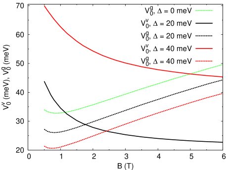
Figure 2: Critical potentials $V^{v}_{0}$ and $V^{g}_{0}$ defined in Eqs. (3) and (4) respectively, as a function of the magnetic field for $\Delta=0$, 20, 40 meV. For $V^{v}_{0}>V^{g}_{0}$ the energy levels in the first Landau gap come from the $K$ valley only, and the lowest energy level in the first Landau gap lies in the middle of this gap with $m=0$. For $\Delta=0$ the potential $V^{v}_{0}$ cannot be defined.

In Fig. 1(b) the energy levels are plotted for $B=1$ T and $\Delta=20$ meV. Now the energy levels are different for the two valleys, but the general characteristics of the energy spectra are similar to those when $\Delta=0$. Discrete energy levels in the mass-induced gap are induced even when $B=0$ but because of the symmetry $E(m,\tau)=E(1-m,-\tau)$ the energies from the two valleys cannot be separated. Furthermore, in a specific device the mass-induced gap is not so easily tunable as the Landau gap and its value is rather sensitive to the specific device configuration. For this reason, the present work is concerned with the energy levels of a quantum dot formed in the first Landau gap which is easily tunable by the magnetic field and can be adjusted at will. In Fig. 1(c) the energy levels are plotted at a higher field, e.g., $B=2$ T but the same $\Delta=20$ meV. Compared to the $B=1$ T spectrum now more levels, corresponding to greater values of $|m|$, are introduced in the first Landau gap. The reason is that by increasing $B$ the states tend to shift nearer the origin thus the effect of the potential well becomes more important and the energies start to deviate from the zeroth Landau level.

For the calculations of the energy spectra the range of angular momentum numbers $m$ is large enough to accurately derive all energies in the considered energy range. The convergence of the energy spectrum for larger values of $V_{0}$ and $B$ requires a broader $m$ range. For example, at $V_{0}=30$ meV and $B=1$ T the $m=-10$ energy level is about 41 $\mu$eV below the zeroth Landau level. When the field increases to $B=2$ T then to a good approximation the same energy difference is observed for $m=-18$.

Figures 1(b) and (c) demonstrate that an interesting energy pattern arises in the first Landau gap provided $V_{0}$ is not too large; for example in Fig. 1(b) for $V_{0}<35$ meV only energy levels from the $K$ valley ($\tau=1$) are relevant. In contrast, for $V_{0}>35$ meV energy levels which come from both valleys lie in the first Landau gap leading to a more complex energy spectrum. Focusing on the first Landau gap, at a fixed $B$ and $\Delta$ there is a critical potential well depth $V^{v}_{0}$, that defines the crossover from the “single-valley” energy spectrum to the “two-valley” spectrum. This effect is rather robust and can be more easily identified when $\Delta$ is large. Since in the experiments the energy gap is usually fixed we below focus on the magnetic field dependence of $V^{v}_{0}$.

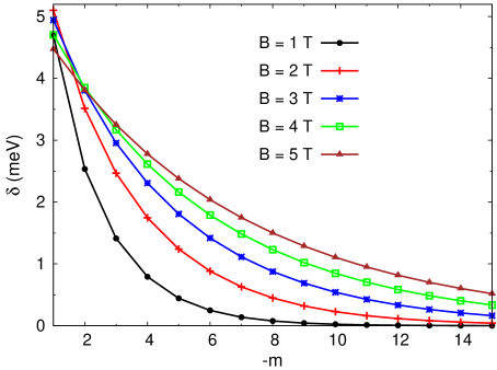
Figure 3: Energy spacing $\delta=E(m,\tau=1)-E(m+1,\tau=1)$ between successive energy levels as a function of the angular momentum number $m$ with $-15\leq m\leq-1$. The magnetic field is $B$, the mass term is $\Delta=40$ meV. The potential is $V_{0}=V^{g}_{0}$, thus by definition $E(m=0,\tau=1)$ is the lowest lying energy in the middle of the first Landau gap.

To explore the energy spectrum in the first Landau gap we first identify the energy level $E(m=0,\tau=-1,V_{0}=0)=+\Delta/2$. By increasing $V_{0}$ this energy level decreases and we define the critical potential $V^{v}_{0}$ which satisfies

$$E(m=0,\tau=-1,V_{0}=V^{v}_{0})=-\Delta/2.$$ (3)

For $V_{0}>V^{v}_{0}$ energies from both valleys lie in the first Landau gap and eventually the spectrum becomes rather complex with many crossing points appearing at random values of $V_{0}$, $B$ due to the broken valley degeneracy. The critical potential $V^{v}_{0}$ can be considered as the maximum allowed value of $V_{0}$ which leads to a single-valley energy spectrum in the first Landau gap. To specify the optimum dot energy range we also need to determine the minimum value of $V_{0}$, consequently, we need to choose a reference ground energy in the first Landau gap. For this purpose we identify the energy level $E(m=0,\tau=1,V_{0}=0)=-\Delta/2$ which decreases with $V_{0}$, and we define the critical potential $V^{g}_{0}$ which satisfies

$$E(m=0,\tau=1,V_{0}=V^{g}_{0})=-\Delta/2-E_{L}/2.$$ (4)

with $E_{L}$ being the value of the first Landau gap as indicated in Fig. 1. This definition of $V^{g}_{0}$ ensures that the lowest level in the first Landau gap lies in the middle of this gap. As a result, when the $B$ field is high enough the few lowest discrete levels are energetically isolated lying far away from the bulk Landau levels.

Both critical potentials $V^{v}_{0}$ and $V^{g}_{0}$ are magnetic field dependent. In Fig. 2 we plot $V^{v}_{0}$ and $V^{g}_{0}$ versus the magnetic field for three values of $\Delta$. The potential $V^{v}_{0}$ decreases as the field increases and the field dependence is rather large for small fields when the difference between the mass-induced gap and the Landau gap is small. In contrast, if the magnetic field is high enough then $V^{v}_{0}$ varies slowly and eventually $V^{v}_{0}\rightarrow\Delta$. For example, our calculations show that at $B=20$ T $V^{v}_{0}\approx 41.5$ meV for $\Delta=40$ meV and $V^{v}_{0}\approx 20.7$ meV for $\Delta=20$ meV. The potential $V^{g}_{0}$ has almost a linear field dependence but for low enough fields ($B<1$ T) the field dependence can be more complicated. This regime is not of particular interest here because of the small value of the Landau gap, which in a realistic sample becomes even smaller due to the level broadening. The energies coming from the two valleys lie in a different energy range provided $V^{v}_{0}>V^{g}_{0}$, and according to Fig. 2 this condition is satisfied only for $B\lesssim 1.7$ T when $\Delta=20$ meV. But, when $\Delta=40$ meV $V^{v}_{0}>V^{g}_{0}$ even when the magnetic field note0 is as high as 6 T. A larger $\Delta$ results in a broader $B$ field range in which $V^{v}_{0}>V^{g}_{0}$. This feature might be advantageous to easily separate the energies from the two valleys and define a dot with a specific valley. However, engineering a large $\Delta$ cannot be guaranteed and, as quantified below, by increasing $\Delta$ both the first Landau gap and the energy spacing between successive levels in the gap decrease. Consequently, a very large $\Delta$ is not necessarily ideal.

To obtain a better insight into the energy spectra we plot in Fig. 3 the energy spacing between successive energy levels $\delta=E(m,\tau=1)-E(m+1,\tau=1)$ lying in the first Landau gap at $V_{0}=V^{g}_{0}$. All the relevant levels correspond to $m\leq 0$ and originate from the $-\Delta/2$ Landau level. According to Fig. 3, for all magnetic fields the largest spacing occurs between the two lowest levels that correspond to $m=0$, $-1$ in order of increasing energy. However, the spacing, in general, can exhibit a strong $B$ dependence for the field range considered; as $B$ increases the spacing tends to increase drastically for large $|m|$ values. For $m=-10$ the spacing is vanishingly small at $B=1$ T, but is about $1$ meV at $B=5$ T. This is due to the fact that larger $|m|$ states are shifted nearer the origin of the well because of the increase of the magnetic barrier so their energies start to deviate significantly from the bulk Landau level $-\Delta/2$. The conclusion is that by tuning the magnetic field the system can be switched from a few-level dot to a many-level dot with an appreciable energy spacing. At $B=4$ T the Zeeman splitting is about $0.46$ meV, for $g=2$ $g$-factor, and $k_{B}T\approx 0.34$ meV at $T=4$ K. These values are much smaller than a typical spacing of $\delta\approx 2-4$ meV, (Fig. 3) allowing the spectroscopy of the dot levels. freitag16 For the results in Fig. 3 the effective width of the potential well is $\sqrt{2}L=40$ nm. Increasing the width to $\sqrt{2}L=80$ nm the $m=0$ energy level lies closer to $-V_{0}$ and the typical energy spacing decreases, e.g., at $B=2-4$ T the spacing between the two lowest levels is about 1.5 meV. The results are only slightly sensitive to the details of the potential well profile maksym provided the effective width of the well remains fixed.

Figure 4: Energy spacing $\delta=E(m=-1,\tau=1)-E(m=0,\tau=1)$ as a function of the mass term $\Delta$ at different fields $B=1$, 3, 5 T. The potential is $V_{0}=V^{g}_{0}$, thus by definition $E(m=0,\tau=1)$ lies in the middle of the first Landau gap. The inset shows the first Landau gap at $B=1$, 3, 5 T.

According to the above analysis for the proper $B$, $V_{0}$ the discrete energies coming from the two valleys can be adjusted in different ranges, and in the first Landau gap only $K$-valley ($\tau=1$) energies can exist; with an energy spacing of a few meV for the low-lying energies. An important issue is how these properties are affected by the mass term $\Delta$. To explore this issue we plot in Fig. 4 the energy spacing $\delta=E(m=-1,\tau=1)-E(m=0,\tau=1)$ as a function of $\Delta$ at three different magnetic fields and $V_{0}=V^{g}_{0}$. A more general $\Delta$ and $V_{0}$ dependence of the energies is presented in Appendix B. In Fig. 4 the condition $V^{v}_{0}>V^{g}_{0}$ is not necessarily satisfied, and only for $\Delta\gtrsim$ 10 meV the energy level $E(m=-1,\tau=1)$ corresponds to the first excited level in the first Landau gap for all the fields considered. For smaller values of $\Delta$ the level $E(m=0,\tau=-1)$ is relevant. As seen in Fig. 4, the energy spacing $\delta$ decreases with $\Delta$ because the effective mass of the carriers increases, therefore the Dirac system starts to resemble a Schrodinger one. At $B=1$ T a mass term of $\Delta\gtrsim 16$ meV is needed to induce only $K$-valley energies in the first Landau gap, i.e., the condition $V^{v}_{0}\gtrsim V^{g}_{0}$ is satisfied. At $B=3$ T the critical value of $\Delta$ increases to $\Delta\gtrsim 26$ meV. Despite this increase the induced Landau gap at $B=3$ T or 5 T (Fig. 4 inset) is still more than twice larger than at $B=1$ T, while the corresponding decrease in $\delta$ is small. As a result at higher magnetic fields the discrete energies of the dot can be put further away from the bulk Landau levels and still $\delta$ can have an appreciable value of $\delta\approx 4$ meV for $\Delta\approx 50$ meV.

In this work, the lowest energy level of the quantum dot is defined in the first Landau gap by the $m=0$ level for $\tau=1$. It is thus useful to explore the variation of this level with respect to the external parameters $V_{0}$ and $B$. As seen in Fig. 1(a) for $\Delta=0$ and $B=1$ T this energy cannot be less than $-V_{0}$. This feature is always valid and the energy difference from the bottom of the well is small when the effective width of the well $L$ is large. Furthermore, as the $B$ field increases the lowest dot energy shifts closer to $-V_{0}$, and eventually the field dependence of the energy becomes weak at high fields when the maximum amplitude of the state occurs in the quantum well region. Some of these trends are quantified in Fig. 5. Specifically, at $V_{0}=50$ meV the $m=0$ energy shifts closer to $-V_{0}$ and changes by over $90\%$ when the field increases from $B=1$ T to $B=3$ T. At $B=5$ T the $m=0$ state is almost entirely localised in the quantum well region, therefore, by further increasing the field to $B=7$ T the corresponding energy changes by less than $5\%$. On the contrary, focusing on $m=-5$, $-10$ and tuning the field from $B=5$ T to 7 T the corresponding energies change by over $28\%$ and $57\%$ respectively. For these values of $m$ small changes in the energy are observed at much higher magnetic fields.

Figure 5: Energies as a function of the potential well for different magnetic fields $B$ and $\tau=1$, $\Delta=40$ meV. All the levels are shifted by $\Delta/2$; $E\rightarrow E+\Delta/2$, thus $E=0$ for $V_{0}=0$. Only energy levels in the first Landau gap are shown, thus $V_{0}$ cannot be taken arbitrarily large; (a) at $B=1$ T and 3 T. The angular momentum number $m$ is indicated in each frame.

Figure 6: Exact and approximate energies as a function of the potential well at $B=5$ T, $\Delta=0$ and different angular momentum numbers $m$.

IV Approximate method

Approximate methods for graphene systems are rather rare in the literature, since the differential equations describing the systems do not usually allow for any simplified assumptions to be made. However, if a simple condition is approximately fulfilled by the two envelope functions $f_{i}$ then some assumptions can be made. This idea is followed here.

Specifically, in this section, we develop an approximate method to determine the $m\leq 0$ energies $E$ which lie in the first Landau gap and satisfy the limit $E\rightarrow 0$ ($-\Delta/2$) when the potential $V\rightarrow 0$. These energies constitute the dot energies of interest studied in Sec. III. The approximation is particularly good in the regime where one of the two components $f_{i}$ dominates. Such a regime occurs when the potential depth is small, and as specified below the small potential depth is related to the angular momentum and the magnetic field.

For the approximate method we start by defining the two functions $f^{\pm}=f_{1}\pm f_{2}$. Using the equations for $f_{i}$ derived in Appendix A [Eqs. (7a) and (7b)] it can be easily shown that $f^{\pm}$ satisfy the two coupled first order differential equations

$$(V+U)f^{+}+\frac{\tau\Delta}{2}f^{-}-\gamma\frac{df^{-}}{dr}=Ef^{+},$$

$$(V-U)f^{-}+\frac{\tau\Delta}{2}f^{+}+\gamma\frac{df^{+}}{dr}=Ef^{-}.$$

To proceed with the approximate method it is more convenient to work with the second order equations

$$\frac{d^{2}f^{+}}{dr^{2}}+\left(\frac{(E-V)^{2}}{\gamma^{2}}-\frac{U^{2}}{\gamma^{2}}-\frac{\Delta^{2}}{4\gamma^{2}}\right)f^{+}-\frac{(U-V)^{\prime}}{\gamma}f^{-}=0,$$

$$\frac{d^{2}f^{-}}{dr^{2}}+\left(\frac{(E-V)^{2}}{\gamma^{2}}-\frac{U^{2}}{\gamma^{2}}-\frac{\Delta^{2}}{4\gamma^{2}}\right)f^{-}-\frac{(U+V)^{\prime}}{\gamma}f^{+}=0,$$

with $(\tau\Delta)^{2}=\Delta^{2}$. If the two functions $f_{1}$, $f_{2}$ are localised in identical regions, or with strong overlap, and a regime can be found satisfying $f_{2}\gg f_{1}$ then $f^{\pm}\approx\pm f_{2}$ and to a good approximation the two equations above decouple. For $\Delta=0$ this condition is exact for the zeroth Landau level because when $V=0$ then $f_{1}=0$ and only $f_{2}\neq 0$. Consequently, if $V\neq 0$ but small enough then we expect the inequality $f_{2}\gg f_{1}$ to be approximately satisfied. In this case, the exact second order equations lead to the following approximate equation for the dominant component $f_{2}$

$$\frac{d^{2}f_{2}}{dr^{2}}+K^{2}_{\pm}f_{2}=0,$$ (5)

and the energy dependent coefficient is

$$K^{2}_{\pm}(r,E)=\frac{(E-V)^{2}}{\gamma^{2}}-\frac{U^{2}}{\gamma^{2}}-\frac{\Delta^{2}}{4\gamma^{2}}+\frac{(U\pm V)^{\prime}}{\gamma}.$$ (6)

The differential Eq. (5) is useful because it has a Schrödinger form. An interesting feature which simplifies the analysis is that $K^{2}_{\pm}$ has no singular point; unlike the coefficient $Q^{2}_{i}$ which appears in the exact Eq. (2) and at $R_{0}$ $Q^{2}_{i}(R_{0})\rightarrow-\infty$ with $V_{\mp}(R_{0})=0$. Therefore, a confined state $f_{2}$ that is a solution to Eq. (5) has an oscillatory amplitude in the spatial region schiff where $K^{2}_{\pm}>0$, and a decaying amplitude where $K^{2}_{\pm}<0$. The latter inequality indicates that for a potential $V$ that rises asymptotically the existence of a confined state depends on the strength of $V$ and $A_{\theta}$, in agreement with a previous work. giavaras09

Considering the quantum dot system, $K^{2}_{\pm}$ as a function of the radial distance $r$ has a positive maximum ($dK^{2}_{\pm}/dr=0$) for all $m$ but zero for which $K^{2}_{\pm}$ diverges at $r=0$. The position of the maximum is sensitive not only to the dot parameters $B$, $V_{0}$, $L$, $m$ but also the dot energy-solution of Eq. (5). When $\Delta=0$ this energy satisfies the physical requirement $E\rightarrow 0$ for $V\rightarrow 0$, i.e., it converges to the zeroth Landau level. The two exact equations satisfied by $f^{\pm}$ have also been applied to potentials $V$ that increase as power laws, and quantum states with large positive values of $m$. Then to a very good approximation giavarasE $f_{1}\approx\pm f_{2}$. This regime is very different from the one examined here resulting in a markedly different energy spectrum.

The solution of Eq. (5) is only slightly sensitive to the sign of the $V^{\prime}$ term, provided $(U\pm V)^{\prime}\approx U^{\prime}$ in the region where $f_{2}$ is localised. This condition can, for example, be satisfied when $B$ is high and simultaneously $V$ is small. The term $(U\pm V)^{\prime}$ however cannot be completely discarded because it can lead to $K^{2}_{\pm}<0$ for all $r$ failing to predict the dot energy. For clarity we consider only $(U-V)^{\prime}$, and to quantify the approximate results we plot in Fig. 6 some approximate energy levels together with the exact ones as a function of the potential depth $V_{0}$. The agreement is very good and the correct $V_{0}$ dependence of the energies is predicted.

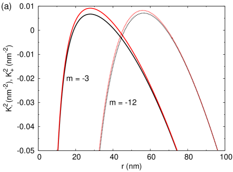
Figure 7: (a) Energy dependent coefficients $K^{2}_{-}$, $K^{2}_{+}$ defined in Eq. (6) in the main text, as a function of the radial coordinate for $B=5$ T, $\Delta=0$, $V_{0}=37$ meV and two values of $m$. The curves shown in black (red) correspond to $K^{2}_{-}$ ($K^{2}_{+}$). [(b), (c)] Turning points $R_{a}$, $R_{b}$ satisfying $K^{2}_{-}(R_{a})=K^{2}_{-}(R_{b})=0$, and singular point $R_{0}$ satisfying $E=V(R_{0})$ for $m=-3$ and $m=-12$ respectively. On the length scale shown the variation of $R_{0}$ is vanishingly small.

The approximation is somewhat better for larger negative values of $m$, but when the absolute energy is very small numerical errors in the computations can change this trend. The error note for the approximate energies plotted in Fig. 6 is about $1-2\%$, and even better agreement is achieved for specific values of $V_{0}$ and $m$. From Fig. 6 we can also extract that the error slightly increases with $V_{0}$, and specifically, in the chosen $V_{0}$ range the increase is about $1\%$. All these trends are consistent with the fact that as $V_{0}$ increases the component $f_{1}$ acquires a larger amplitude so the basic assumption $f_{2}\gg f_{1}$ becomes gradually less accurate especially when $|m|$ is small. The agreement with the exact numerical energies is better when the effective width $L$ of the quantum well increases, and as a result the term $V^{\prime}$ decreases in the well region. For $\sqrt{2}L=80$ nm the maximum error for the same parameter values shown in Fig. 6 is less than $1\%$, and small errors of the order of $0.1\%$ can be achieved. The key idea behind the approximation is that the two components $f_{i}$ are localised in nearly the same regions but one of the two components dominates. The latter condition is well satisfied at high $B$, small $V_{0}$ and large $L$.

The position of the singular point that appears in the exact Eq. (2) but not in the approximate Eq. (6) deserves some further investigation. The fact that there is no singular point in the approximate Eq. (6) does not necessarily imply that the singular point is located (far) away from the region where $f_{2}$ is localised, and can be ignored. To quantify this argument we plot in Fig. 7(a) the coefficient $K^{2}_{\pm}(r)$ versus the radial coordinate for the parameters $B=5$ T, $\Delta=0$ and $V_{0}=37$ meV. The function $f_{2}$ is localised in the region where $K^{2}_{\pm}(r)>0$, and this region shifts away from the origin for larger values of $m$, in agreement with the behaviour exhibited by the Landau states. Because $K^{2}_{+}(r)$ is not very different from $K^{2}_{-}(r)$, we consider for simplicity only $K^{2}_{-}(r)$ and define the two “turning” points $R_{a}$, $R_{b}$ with $K^{2}_{-}(R_{a})=K^{2}_{-}(R_{b})=0$, $R_{b}>R_{a}$. In Figs. 7(b) and (c) we plot $R_{a}$, $R_{b}$ together with the singular point $R_{0}$ of Eq. (2) satisfying $E=V(R_{0})$. For each value of $V_{0}$ the condition $R_{a}<R_{0}<R_{b}$ is satisfied, indicating that $R_{0}$ occurs within the region where $f_{2}$ is localised and has large amplitude. The conclusion from the two examples illustrated in Figs. 7(b) and (c) is that the approximate method is applicable to the regime where $R_{0}$ cannot be ignored in the exact Eq. (2). The occurrence of $R_{0}$ is needed to give rise to a non-zero $f_{1}$, when $V_{0}\neq 0$, in approximately the same region as that where $f_{2}$ is localised. The fact that $R_{0}$ depends only weakly on $V_{0}$ [Figs. 7(b) and 7(c)] indicates that some further approximations can be made. Investigation of the numerically exact values of $R_{0}$ shows that $R_{0}\approx R$ for some values of $m$, where $R=\sqrt{(2|m|+1)\hbar/eB}$ is the peak position of $f_{2}$ when $V_{0}=0$. Then $E$ can be determined analytically, $E\approx V(R)$, but quantifying this approximation is beyond the scope of this paper.

Finally, based on the assumptions behind the approximate method, it can be easily demonstrated that the method can be applied equally well to quantum dot potentials which continuously increase, e.g., $V(r)=V_{g}r^{n}$, with $n>0$ and $V_{g}>0$. However, in this case the physics is different from a potential that is asymptotically constant. The reason is that the energy deviation from the zeroth Landau level increases with $|m|$, as the Landau states which are localised away from the origin are affected more by the potential $V(r)$. For completeness one example for this case is presented in Appendix C.

V Conclusions

In summary, we considered a graphene sheet in a perpendicular magnetic field and explored the energy spectrum of a quantum dot formed in the first Landau gap. The discrete levels of the quantum dot emerge from the Landau levels using a potential well which can be experimentally realised and efficiently tuned with an STM tip. freitag16 ; freitag18

In our graphene system the valley degeneracy is broken and as a result the dot energy spectrum can be rather complex exhibiting many irregular level crossings and small energy spacings which are sensitive to the applied fields. However, as demonstrated in this work in the first Landau gap and for the appropriate potential well, magnetic field, and mass-induced gap the dot energy spectrum can have a simple pattern with discrete energies coming from one of the two valleys only. In this part of the spectrum there are no energy crossings and the lowest energy level corresponds to $m=0$ angular momentum, while $m$ successively decreases by $-1$ for each higher energy level.

The magnetic field dependence of the energy levels and the effect of the mass term were examined. It was shown that the discrete energies of the dot in the first Landau gap lie away from the bulk Landau levels and the typical energy spacing can be large enough, of a few meV, when the magnetic field is $3-5$ T, and the mass-induced gap is about 50 meV. It was demonstrated that in the regime where one of the two components of the Dirac state dominates an approximate method can be developed. Within this method a Schrödinger equation was derived which can predict the region where the dominant component is localised. The approximate energies for states with negative angular momentum exhibit the correct general trends and are in a good agreement with the exact energies.

The graphene system studied here is experimentally realizable and the simple energy patterns that were identified arise in a realistic range of fields. The results of this work could guide further investigations of confined states in two dimensional materials.

Appendix A Quantum dot equations

The equations describing a graphene quantum dot in the continuum approximation have been derived in various previous works. giavaras12 ; giavaras11 In brief, the eigenvalue problem defined in Eq. (1) in the main text can be reduced to two equations for the radial functions $f_{i}$. This is done with the substitution giavaras12 ; giavaras11 $\Psi(r,\theta)=(f_{1}(r)\exp[i(m-1)\theta]$, $if_{2}(r)\exp[im\theta])/\sqrt{r}$ which leads to

$$(V+\tau\Delta/2)f_{1}+\left(U+\gamma\frac{d}{dr}\right)f_{2}=Ef_{1},$$ (7a)

$$\left(U-\gamma\frac{d}{dr}\right)f_{1}+(V-\tau\Delta/2)f_{2}=Ef_{2},$$ (7b)

where

$$U=\gamma\frac{2m-1}{2r}+\gamma\frac{eA_{\theta}}{\hbar},$$

includes the terms due to the angular motion and the magnetic vector potential. For convenience we set $V_{\pm}=V-E\pm\tau\Delta/2$ and use these two equations to derive the decoupled equations for each radial envelope function $f_{i}$

$$\frac{d^{2}f_{1}}{dr^{2}}-\frac{V^{{}^{\prime}}}{V_{-}}\frac{df_{1}}{dr}+\left(-\frac{U^{2}}{\gamma^{2}}-\frac{U^{{}^{\prime}}}{\gamma}+\frac{U}{\gamma}\frac{V^{{}^{\prime}}}{V_{-}}+\frac{V_{-}V_{+}}{\gamma^{2}}\right)f_{1}=0,$$

$$\frac{d^{2}f_{2}}{dr^{2}}-\frac{V^{{}^{\prime}}}{V_{+}}\frac{df_{2}}{dr}+\left(-\frac{U^{2}}{\gamma^{2}}+\frac{U^{{}^{\prime}}}{\gamma}-\frac{U}{\gamma}\frac{V^{{}^{\prime}}}{V_{+}}+\frac{V_{-}V_{+}}{\gamma^{2}}\right)f_{2}=0,$$

where prime denotes differentiation with respect to $r$. These two equations have the general compact form

$$\frac{d^{2}f_{i}}{dr^{2}}+a_{i}\frac{df_{i}}{dr}+b_{i}f_{i}=0,$$

with $i=1$, 2 and the coefficients $a_{i}$, $b_{i}$ can be inferred. We assume giavaras11 $f_{i}=g_{i}y_{i}$ and derive that

$$g_{i}\frac{d^{2}y_{i}}{dr^{2}}+(2g^{{}^{\prime}}_{i}+a_{i}g_{i})\frac{dy_{i}}{dr}+(g^{{}^{\prime\prime}}_{i}+a_{i}g^{{}^{\prime}}_{i}+b_{i}g_{i})y_{i}=0.$$

We choose $g^{{}^{\prime}}_{i}/g_{i}=-a_{i}/2$ to derive the final equation for $y_{i}$: $d^{2}y_{i}/dr^{2}+Q^{2}_{i}y_{i}=0$. The coefficient $Q^{2}_{i}(r,E)$ is given in Eq. (2) in the main text.

Appendix B Effect of mass term on dot levels

In the main text, it was shown that in the appropriate range of parameters the $m=0$, $-1$ energy levels for $\tau=1$ can define the two lowest levels of the quantum dot in the first Landau gap. Figure 8 shows the effect of the mass term $\Delta$ on these levels for different magnetic fields. At low magnetic fields the value of $\Delta$ is important, especially at large $V_{0}$ values which approach the Landau gap. However, as the field increases the two levels exhibit a smaller $\Delta$ dependence, until eventually a shift of around $\Delta/2$ is observed. These trends are in agreement with the change in the corresponding energy spacing versus $\Delta$ shown in Fig. 4 in the main text.

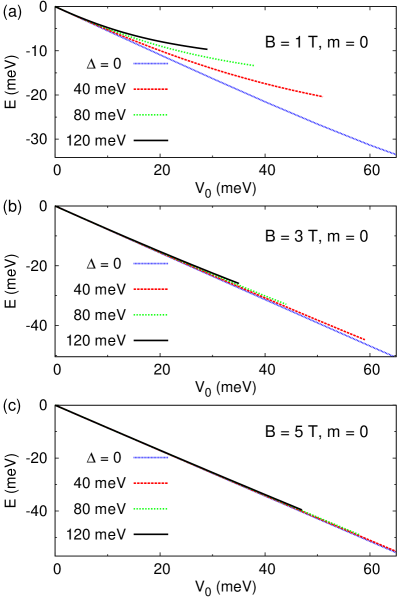
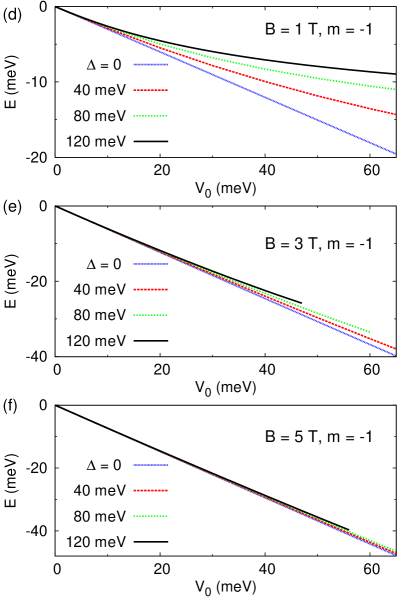
Figure 8: Energy levels as a function of the potential well for different mass terms $\Delta$ and $\tau=1$. For a better comparison all the levels are shifted by $\Delta/2$; $E\rightarrow E+\Delta/2$, thus $E=0$ for $V_{0}=0$. Only energy levels in the first Landau gap are shown, thus $V_{0}$ cannot be taken arbitrarily large. The angular momentum number $m$ and the $B$ field are indicated in each frame.

Figure 9: Exact and approximate energies as a function of the potential well at $B=5$ T, $\Delta=0$ and different angular momentum numbers $m$. The quantum dot potential is $V(r)=V_{g}r/x$, with $x=800$ nm.

Appendix C Model quantum dot potential

To demonstrate the efficacy of the approximate method described in the main text, we here study a model quantum dot potential. This is defined by the potential well $V(r)=V_{g}r/x$, with $x=800$ nm. Figure 9 illustrates the exact and approximate energies as a function of $V_{g}$ for different angular momentum $m$. The overall agreement is excellent and the error is less than $0.1\%$; depending on the parameters it can be even an order of magnitude smaller. Similar to Figs. 7(b) and (c) in the main text, the condition $R_{a}<R_{0}<R_{b}$ is again satisfied. This demonstrates the importance of the singular point $R_{0}$ when $V_{g}\neq 0$.

References

- (1) N. M. Freitag, L. A. Chizhova, P. N. Incze, C. R. Woods, R. V. Gorbachev, Y. Cao, A. K. Geim, K. S. Novoselov, J. Burgdorfer, F. Libisch, and M. Morgenstern, Nano Lett. 16, 5798 (2016).
- (2) N. M. Freitag, T. Reisch, L. A. Chizhova, P. N. Incze, C. Holl, C. R. Woods, R. V. Gorbachev, Y. Cao, A. K. Geim, K. S. Novoselov, J. Burgdorfer, F. Libisch, and M. Morgenstern, Nat. Nanotech. 13, 392 (2018).
- (3) S. Y. Li, Y. N. Ren, Y. W. Liu, M. X. Chen, H. Jiang, and L. He, 2D Mater. 6, 031005 (2019).
- (4) J. Lee, D. Wong, J. Velasco Jr, J. F. R. Nieva, S. Kahn, H. Z. Tsai, T. Taniguchi, K. Watanabe, A. Zettl, F. Wang, L. S. Levitov, and M. F. Crommie, Nat. Phys. 12, 1032 (2016).
- (5) J. B. Qiao, H. Jiang, H. Liu, H. Yang, N. Yang, K. Y. Qiao, and L. He, Phys. Rev. B 95, 081409(R) (2017).
- (6) A. V. Rozhkov, G. Giavaras, Y. P. Bliokh, V. Freilikher, and F. Nori, Phys. Rep. 503, 77 (2011).
- (7) R. Balog, , Nat. Mater. 9, 315 (2010).
- (8) W. X. Wang, L. J. Yin, J. B. Qiao, T. Cai, S. Y. Li, R. F. Dou, J. C. Nie, X. Wu, and L. He, Phys. Rev. B 92, 165420 (2015).
- (9) S. Y. Zhou, G. H. Gweon, A. V. Fedorov, P. N. First, W. A. de Heer, D. H. Lee, F. Guinea, A. H. C. Neto, and A. Lanzara, Nat. Mater. 6, 770 (2007).
- (10) X. Fan, Z. Shen, A. Q. Liu, and J. L. Kuo, Nanoscale 4, 2157 (2012).
- (11) P. Shemella and S. K. Nayak, Appl. Phys. Lett. 94, 032101 (2009).
- (12) J. R. Schaibley, H. Yu, G. Clark, P. Rivera, J. S. Ross, K. L. Seyler, W. Yao, and X. Xu, Nat. Rev. Mat. 1, 16055 (2016).
- (13) V. D. Karanikolas and E. Paspalakis, Phys. Rev. B 96, 041404(R) (2017).
- (14) G. Giavaras, P. A. Maksym, and M. Roy, J. Phys.: Condens. Matter 21, 102201 (2009).
- (15) G. Giavaras and F. Nori, Phys. Rev. B 85, 165446 (2012).
- (16) S. Moriyama, Y. Morita, E. Watanabe, D. Tsuya, Appl. Phys. Lett. 104, 053108 (2014).
- (17) H. M. Abdullah, H. Bahlouli, F. M. Peeters, and B. Van Duppen, J. Phys.: Condens. Matter 30, 385301 (2018).
- (18) S. Caneva, M. Hermans, M. Lee, A. G. Fuente, K. Watanabe, T. Taniguchi, C. Dekker, J. Ferrer, H. S. J. van der Zant, and P. Gehring, Nano Lett. 20, 4924 (2020).
- (19) I. Keren, T. Dvir, A. Zalic, A. Iluz, D. LeBoeuf, K. Watanabe, T. Taniguchi, and H. Steinberg, Nat. Commun. 11, 3408 (2020).
- (20) P. Recher, J. Nilsson, G. Burkard, and B. Trauzettel, Phys. Rev. B 79, 085407 (2009).
- (21) V. Jakubsky and D. Krejcirik, Ann. Phys. (N. Y.) 349, 268 (2014).
- (22) M. Sadrara and M. F. Miri, Phys. Rev. B 99, 155432 (2019).
- (23) G. Giavaras and F. Nori, Phys. Rev. B 83, 165427 (2011).
- (24) B. S. Kandemir and G. Omer, The Eur. Phys. J. B 86, 299 (2013).
- (25) P. A. Maksym, M. Roy, M. F. Cracium, M. Yamamoto, S. Tarucha, and H. Aoki, J. Phys.: Conf. Ser. 245, 012030 (2010).
- (26) C. Gold, A. Kurzmann, K. Watanabe, T. Taniguchi, K. Ensslin, and T. Ihn, Phys. Rev. Research 2, 043380 (2020).
- (27) S. Y. Li, Y. Su, Y. N. Ren, and L. He, Phys. Rev. Lett. 124, 106802 (2020).
- (28) D. Walkup, F. Ghahari, C. Gutierrez, K. Watanabe, T. Taniguchi, N. B. Zhitenev, and J. A. Stroscio, Phys. Rev. B 101, 035428 (2020).
- (29) G. Giavaras and F. Nori, Appl. Phys. Lett. 97, 243106 (2010).
- (30) C. Schattauer, L. Linhart, T. Fabian, T. Jawecki, W. Auzinger, and F. Libisch, Phys. Rev. B 102, 155430 (2020).
- (31) M. Mirzakhani, M. Zarenia, S. A. Ketabi, D. R. da Costa, and F. M. Peeters, Phys. Rev B 93, 165410 (2016).
- (32) M. Y. Li, C. H. Chen, Y. Shi, and L. J. Li, Materialstoday 19, 322 (2016).
- (33) D. N. Le, V. H. Le, and P. Roy, J. Phys.: Condens. Matter 32, 385703 (2020).
- (34) Here, at T.
- (35) L. I. Schiff, Quantum Mechanics (McGraw-Hill, New York, 1968).
- (36) G. Giavaras, P. A. Maksym, and M. Roy, Physica E 42, 715 (2010).
- (37) For the error is about , whereas when nm the error is less than .