Similar Scale-invariant Behaviors between Soft Gamma-ray Repeaters and An Extreme Epoch from FRB 121102

Abstract

The recent discovery of a Galactic fast radio burst (FRB) associated with a hard X-ray burst from the soft gamma-ray repeater (SGR) J1935+2154 has established the magnetar origin of at least some FRBs. In this work, we study the statistical properties of soft gamma-/hard X-ray bursts from SGRs 1806–20 and J1935+2154 and of radio bursts from the repeating FRB 121102. For SGRs, we show that the probability density functions for the differences of fluences, fluxes, and durations at different times have fat tails with a $q$-Gaussian form. The $q$ values in the $q$-Gaussian distributions are approximately steady and independent of the temporal interval scale adopted, implying a scale-invariant structure of SGRs. These features indicate that SGR bursts may be governed by a self-organizing criticality (SOC) process, confirming previous findings. Very recently, 1652 independent bursts from FRB 121102 have been detected by the Five-hundred-meter Aperture Spherical radio Telescope (FAST). Here we also investigate the scale-invariant structure of FRB 121102 based on the latest observations of FAST, and show that FRB 121102 and SGRs share similar statistical properties. Given the bimodal energy distribution of FRB 121102 bursts, we separately explore the scale-invariant behaviors of low- and high-energy bursts of FRB 121102. We find that the $q$ values of low- and high-energy bursts are different, which further strengthens the evidence of the bimodality of the energy distribution. Scale invariance in both the high-energy component of FRB 121102 and SGRs can be well explained within the same physical framework of fractal-diffusive SOC systems.

1 Introduction

Self-organized criticality (SOC; Katz 1986; Bak et al. 1987; Aschwanden et al. 2016) has been found in dynamical behaviors of astrophysics systems. We here examine two types of transient phenomena, namely, soft gamma-ray repeaters (SGRs) and fast radio bursts (FRBs), which have been shown to be associated with each other in at least one case (Zhang, 2020).

Magnetars are highly magnetized neutron stars that exhibit dramatic variability over a broad range of timescales (Duncan & Thompson 1992; Kouveliotou et al. 1998, see also Turolla et al. 2015; Kaspi & Beloborodov 2017 for reviews). Many magnetars were first observed as SGRs, i.e., sources of repeated bursts of soft gamma-/hard X-rays, with typical durations of $\sim 0.1-1$ s and peak luminosities of $\sim 10^{39}-10^{41}$ erg $\rm s^{-1}$. Three several-minute-long giant flares with peak luminosities up to $\sim 10^{44}-10^{47}$ erg $\rm s^{-1}$ have also been observed from three different SGRs (Mazets et al., 1979; Hurley et al., 1999; Palmer et al., 2005). Both bursts and flares are believed to be powered by the dissipation and decay of the ultrastrong magnetic fields, either through neutron star crustquakes (Thompson & Duncan, 1995) or magnetic reconnection (Lyutikov, 2003).

Several works have found that the energy distribution of SGR bursts can be well fitted by a power-law function (e.g., Cheng et al. 1996; Göǧüş et al. 1999, 2000; Prieskorn & Kaaret 2012; Cheng et al. 2020). Power-law size distributions of extreme events can be explained by the concept of SOC in slowly driven nonlinear dissipative systems (Bak et al., 1987; Aschwanden et al., 2016). The SOC subsystems will self-organize, owing to some driving force, to a critical state, at which a small local disturbance can produce an avalanche-like chain reaction of any size within the system (Bak et al., 1987). The fundamental property of all SOC systems have in common is the emergence of scale-free power-law size distributions (Aschwanden, 2011, 2012, 2015; Wang & Dai, 2013; Lyu et al., 2020, 2021). Given the earthquake-like power-law energy distributions, Göǧüş et al. (1999) suggested, for the first time, that systems responsible for SGR bursts are in a SOC state. The earthquake-like behavior also suggests that the energies of SGRs originate from starquakes of magnetars (Duncan & Thompson, 1992; Thompson & Duncan, 1995).

Besides the power-law size distribution, another hallmark of SOC systems is the scale invariance of the avalanche size differences (Caruso et al., 2007; Wang et al., 2015). Caruso et al. (2007) showed that the probability density functions (PDFs) for the earthquake energy differences at different times have fat tails with a $q$-Gaussian form, which could be well explained by introducing a small-world topology on the Olami-Feder-Christensen (OFC) model (Olami et al., 1992). In physics, the OFC model is one of the most popular models displaying SOC. The $q$-Gaussian distribution was then suggested as an important character for describing the presence of criticality (Caruso et al., 2007). Moreover, the form of the PDF does not depend on the time interval adopted for the earthquake energy difference, i.e., the $q$ values in $q$-Gaussian distributions keep nearly constant for different scale intervals, which indicates that there is a scale-invariant structure in the energy differences of earthquakes (Caruso et al., 2007; Wang et al., 2015). Subsequently, Chang et al. (2017) studied 384 X-ray bursts observed in three active episodes of SGR J1550–5418 and found that this SGR shows similar scale-invariant behaviors, i.e., the PDFs of the differences of fluences, peak fluxes, and durations exhibit a common $q$-Gaussian distribution at different scale intervals.

FRBs are intense millisecond-duration bursts of radio waves occurring in the universe (Lorimer et al., 2007; Petroff et al., 2019; Cordes & Chatterjee, 2019). So far, more than 600 FRBs have been reported, and over two dozens of them have been seen to repeat (e.g., Spitler et al. 2016; CHIME/FRB Collaboration et al. 2019; Fonseca et al. 2020; The CHIME/FRB Collaboration et al. 2021). Although rapid developments have been made in the FRB research field, the physical origin of FRBs remains mysterious (Platts et al., 2019; Zhang, 2020; Geng et al., 2021; Xiao et al., 2021). Magnetars have been proposed as the likely engine to power repeating FRBs (Popov & Postnov, 2010; Kulkarni et al., 2014; Murase et al., 2016; Katz, 2016; Metzger et al., 2017; Wang & Yu, 2017; Beloborodov, 2017; Kumar et al., 2017; Yang & Zhang, 2018; Wadiasingh & Timokhin, 2019; Cheng et al., 2020; Wang et al., 2020). On 2020 April 28, one FRB-like event was independently detected by the Canadian Hydrogen Intensity Mapping Experiment (CHIME/FRB Collaboration et al., 2020) and the Survey for Transient Astronomical Radio Emission 2 (Bochenek et al., 2020) in association with a hard X-ray burst from the Galactic magnetar SGR J1935+2154 during its active phase (Li et al., 2021a; Mereghetti et al., 2020; Ridnaia et al., 2021; Tavani et al., 2021). This discovery strongly supports that magnetar engines can produce at least some extragalactic FRBs.

Recently, by analyzing 93 bursts from the repeating FRB 121102 by the observation of the Green Bank Telescope at 4–8 GHz (Zhang et al., 2018), Lin & Sang (2020) found that FRB 121102 has the property of scale invariance similar to that of SGR J1550–5418. During an extreme episode of bursts, FRB 121102 produced 1652 detectable events within a time-span of 62 days (Li et al., 2021b). The peak burst rate reached 117 hr^-1. Such a range of cadence facilitate further investigation into the SOC structures of this source. Another key feature of this burst set from FRB 121102 is the bimodal energy distribution of the burst rate.

Among the 16 known SGRs (12 confirmed and 4 candidates; Olausen & Kaspi 2014), SGR J1550–5418 is the only source to date that has been used to investigate the scale-invariant property (Chang et al., 2017). So it is interesting to know whether other SGRs (e.g., SGR 1806–20 and SGR J1935+2154) share the same property. The magnetar research group at Sabancı University presented their systematic temporal and broad-band spectral analysis of over 1,500 bursts from SGR J1550–5418, SGR 1900+14, and SGR 1806–20 observed with the Rossi X-ray Timing Explorer (RXTE; e.g., Kırmızıbayrak et al. 2017). In these public data, SGR 1806–20 has the largest burst sample (924 bursts), which will be used in our following analysis. Additionally, since SGR J1935+2154 is the first source that has been reported to power a Galactic FRB (CHIME/FRB Collaboration et al., 2020; Bochenek et al., 2020), we will also investigate the physical connection between SGR J1935+2154 and repeating FRBs.

In this paper, we investigate the scale-invariant behaviors of SGR 1806–20, SGR J1935+2154, and FRB 121102. For SGRs, the PDFs of the differences of fluences (or total counts), peak fluxes (or peak counts), and durations at different time scales are shown in Section 2. These PDFs can be well fitted by a $q$-Gaussian function, and the functional form does not depend on the scale interval adopted. In Section 3, we compare the PDFs between SGRs and repeating FRB 121102. The evidence that may shed light on the bimodal burst energy distribution of FRB 121102 is discussed in Section 4. Lastly, a brief summary and discussion are given in Section 5.

2 Scale-invariance in SGRs

2.1 Data

The magnetar research group at Sabancı University has constructed an online database of magnetar bursts detected by the RXTE between 1996 and 2011, which can be visited at http://magnetars.sabanciuniv.edu. This database contains 924 bursts from SGR 1806–20, representing the largest sample for a single observation. The trigger time, total counts, peak counts, and duration of each burst are available in the database.

For SGR J1935+2154, the bursts observed by the Gamma-ray Burst Monitor (GBM) onboard the Fermi satellite during the source’s six active episodes from 2014 to 2020 are used (Lin et al., 2020b, a). The number of bursts is 260. The available information for each burst include trigger time, fluence, and duration, but not peak flux.

The 924 bursts from SGR 1806–20 were all observed with the RXTE/Proportional Counter Array (PCA), and the 260 bursts from SGR J1935+2154 were all observed with the Fermi/GBM. These two instruments are different in numerous ways, including energy passband, sensitivity, background level, etc. The comparison of total counts detected with a pointing instrument, RXTE/PCA (effectively sensitive to 3–30 keV photons) to fluences of an all-sky monitor, GBM (8–200 keV) has to be handled with care. A conversion factor between each PCA count and GBM fluence, in principle, has to be determined (Göǧüş et al., 1999, 2000, 2001). On the other hand, since we are interest in the statistical distribution of the total count differences at different time intervals (see more below), the difference between two PAC counts may be approximated as the difference between two GBM fluences.

The adopted durations of all bursts from both SGR 1806–20 and SGR J1935+2154 were determined by a Bayesian block algorithm, but the sensitivity of detecting instruments are expected to affect the resulting duration distributions. Thus, there is a caveat that the comparison of the PDFs of the duration differences between SGR 1806–20 and SGR J1935+2154 may be affected by the sensitivity of different instruments. Note that Chang et al. (2017) studied the statistical properties of a sample of 384 SGR J1550–5418 bursts detected with the Fermi/GBM. With the same detecting instrument, the duration comparison between SGR J1935+2154 and SGR J1550–5418 would be credible. Here we estimate the waiting time between two adjacent bursts through $\Delta t=t_{i+1}-t_{i}$, where $t_{i+1}$ and $t_{i}$ are the trigger times of the $(i+1)$-th and $i$-th bursts, respectively. As both SGR 1806–20 and SGR J1935+2154 consist of several isolated epochs, we discard the waiting time between the last burst of a certain epoch and the first burst of the next epoch.

Table 1: The mean values of $q$ in the $q$-Gaussian distribution for earthquakes, SGRs, and FRB 121102

Phenomena	Energy range (erg)	Number	$q$-fluence (energy)	$q$-flux	$q$-duration	References
earthquakes		400,000	$1.75\pm 0.15$	–	–	Caruso et al. (2007)
SGR J1550–5418		384	$2.41\pm 0.29$	$2.40\pm 0.30$	$2.06\pm 0.23$	Chang et al. (2017)
SGR 1806–20		924	$2.72\pm 0.05$	$2.65\pm 0.05$	$2.48\pm 0.05$	This work
SGR J1935+2154		260	$2.78\pm 0.12$	–	$2.28\pm 0.15$	This work
FRB 121102	Overall bursts	1652	$2.51\pm 0.03$	$2.50\pm 0.03$	$1.42\pm 0.04$	This work
	with $4\times 10^{36}<E<8\times 10^{39}$
FRB 121102	Low-energy bursts	1253	$1.63\pm 0.09$	$1.81\pm 0.05$	$1.39\pm 0.06$	This work
	with $4\times 10^{36}<E\leq 2\times 10^{38}$
	High-energy bursts	399	$2.21\pm 0.10$	$2.34\pm 0.09$	$1.50\pm 0.16$	This work
	with $2\times 10^{38}<E<8\times 10^{39}$

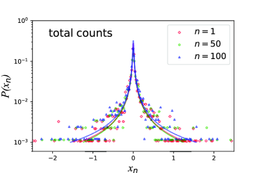
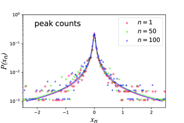
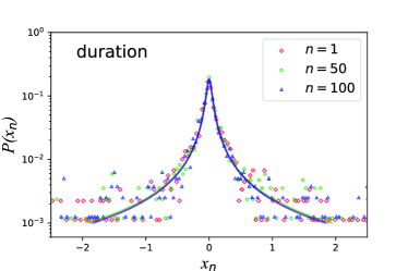
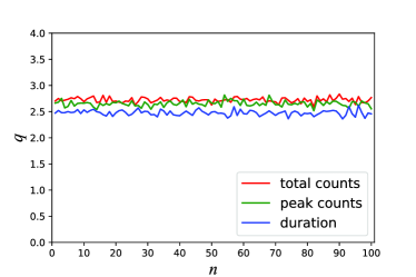
Figure 1: Scale-invariant structure of SGR 1806–20. PDFs of the differences of total counts (upper-left panel), peak counts (upper-right panel), and durations (lower-left panel) for $n=1$ (red diamonds), $n=50$ (green circles), and $n=100$ (blue triangles), and the best-fitting $q$-Gaussian distributions (solid lines). Lower-right panel: the best-fitting $q$ values in the $q$-Gaussian distribution as a function of $n$.

2.2 PDFs of the Avalanche Size Differences

We are now in position to use the data of SGR 1806–20 and SGR J1935+2154 to investigate the PDFs of the avalanche size differences. The difference between two avalanche sizes is given by

$$X_{n}=S_{i+n}-S_{i}\;,$$ (1)

where $S_{i}$ is the size (fluence, peak flux, duration, or waiting time) of the $i$-th burst in temporal order and $n$ (an integer) is the temporal interval scale. In practice, $X_{n}$ is normalized to

$$x_{n}=\frac{X_{n}}{\sigma_{X_{n}}}\;,$$ (2)

where $\sigma_{X_{n}}$ is the standard deviation of $X_{n}$. We are interest in the statistical distribution of $x_{n}$.

Figure 1 shows the statistical results of SGR 1806–20. In this plot, we display the PDFs of the differences of total counts (upper-left panel), peak counts (upper-right panel), and durations (lower-left panel) for $n=1$ (diamonds), $n=50$ (circles), and $n=100$ (triangles). Following Chang et al. (2017), the data are binned based on the Freedman-Diaconis rule (Freedman & Diaconis, 1981). One can see from Figure 1 that these PDFs $P(x_{n})$ have a sharp peak and fat tails, which are different from Gaussian behaviors. The sharp peak means that small size differences are most likely to happen, while the fat tails suggest that there are rare but relatively large size differences. The large fluctuations presented in the tails are caused by the incompleteness given from the lack sampling of small magnitude events at the global scale (Caruso et al., 2007). Additionally, the data points in Figure 1 are almost independent of the temporal interval scale $n$ adopted for the avalanche size difference, indicating a common form of $P(x_{n})$. Here we use the Tsallis $q$-Gaussian function (Tsallis, 1988; Tsallis et al., 1998)

$$f(x_{n})=\alpha\left[1-\left(1-q\right)x_{n}^{2}/\beta\right]^{\frac{1}{1-q}}$$ (3)

to fit $P(x_{n})$, where $\alpha$, $\beta$, and $q$ are free parameters. When $q\rightarrow 1$, the $q$-Gaussian distribution reduces to the Gaussian distribution with mean zero and standard deviation $\sigma=\sqrt{\beta/2}$. Thus, $q\neq 1$ denotes a departure from Gaussian statistics.

The best-fitting parameters ($\alpha$, $\beta$, and $q$) are obtained by minimizing the $\chi^{2}$ statistics,

$$\chi^{2}=\sum_{i}\frac{\left[f(x_{n,i})-P(x_{n,i})\right]^{2}}{\sigma_{P,i}^{2}}\;,$$ (4)

where $\sigma_{P,i}=\sqrt{N_{{\rm bin},i}}/N_{\rm tot}$ is the uncertainty of the data point, with $N_{{\rm bin},i}$ is the event number in the $i$-th bin and $N_{\rm tot}$ is the total number of $x_{n}$. We use the python implementation, emcee (Foreman-Mackey et al., 2013), to apply the Markov Chain Monte Carlo method to derive the best-fitting values and their corresponding uncertainties for these parameters. In Figure 1, the red, green, and blue smooth curves correspond to the best-fitting results for $n=1$, $n=50$, and $n=100$, respectively. We may see that the PDFs of the differences of total counts, peak counts, and durations are well fitted by the $q$-Gaussian function, and that the three curves in each panel overlap almost completely. However, the PDF of the waiting time differences can not be well fitted by $q$-Gaussian (see also Chang et al. 2017), so we do not exhibit it in the figure. The waiting time shows different behaviors, which may be due to the discontinuous observations of the telescope.

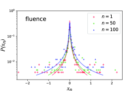
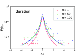
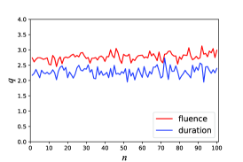
Figure 2: Scale-invariant structure of SGR J1935+2154. PDFs of the differences of fluences (left panel) and durations (middle panel) for $n=1$ (red diamonds), $n=50$ (green circles), and $n=100$ (blue triangles), and the best-fitting $q$-Gaussian distributions (solid lines). Right panel: the best-fitting $q$ values in the $q$-Gaussian distribution as a function of $n$.

Furthermore, we compute the PDFs of the differences of total counts, peak counts, and durations at different scale intervals $1\leq n\leq 100$, and fit the PDFs with the $q$-Gaussian function. In the lower-right panel of Figure 1, we plot the best-fitting $q$ values as a function of $n$. We find that the $q$ values are approximately invariant for different scale intervals $n$. The property of the independence of $q$ values on $n$ is referred to as scale invariance. The mean values of $q$ for total counts, peak counts, and duration are $2.72\pm 0.05$, $2.65\pm 0.05$, and $2.48\pm 0.05$, respectively, which are summarized in Table 1. Here the uncertainty denotes the standard deviation of $q$. Interestingly, the $q$ values we find here are close to the values derived from SGR J1550–5418 (Chang et al., 2017), which indicates that there is a common scale-invariant property in SGRs.

Similar results can be obtained for the data of SGR J1935+2154, see Figure 2. The $q$ values for this data also keep approximately steady for different scale intervals $n$. The mean values of $q$ for fluence and duration are $2.78\pm 0.12$ and $2.28\pm 0.14$, respectively. As shown in Table 1, these values are well consistent with those of SGR J1550–5418 (Chang et al., 2017) and SGR 1806–20, supporting a common scale-invariant structure of SGRs again.

It is worth mentioning that our statistic relies on the size difference between two successive events. However, both RXTE and Fermi are low orbit instruments and the sources of interest would frequently be blocked by the Earth. It may happen that there are other bursts in between some of those events listed in the literature, and not recorded because the sources were occulted. Moreover, there are also some unresolved weak bursts in the data. We have proved that for the successive burst data, by changing the time interval $n$, or by reshuffling the time series, no change in the PDFs of the size differences is observed. In other words, the scale-invariant behaviors of SGRs are only weakly sensitive to the absence of the obscured bursts or the unresolved weak bursts.

3 Comparison with FRB 121102

Owing to the association between FRB 200428 and an X-ray burst from the Galactic magnetar SGR J1935+2154 (CHIME/FRB Collaboration et al., 2020; Bochenek et al., 2020; Li et al., 2021a; Mereghetti et al., 2020; Ridnaia et al., 2021; Tavani et al., 2021), it is natural to consider whether radio bursts of repeating FRBs have a similar scale-invariant behavior. In this section, we compare the PDFs between SGRs and repeating FRBs.

Recently, Li et al. (2021b) reported the detection of 1652 independent bursts in 59.5 hours spanning 62 days using the Five-hundred-meter Aperture Spherical radio Telescope (FAST; Nan et al. 2011; Li et al. 2018) at 1.05–1.45 GHz. Such a uniform sample prevent complex selection effects, which can be introduced by different instruments and different frequency bands used in observations. Here we focus on the PDFs for the differences of energies, fluxes, and durations at different time scales. For a fixed $n$, we fit the PDF with the $q$-Gaussian function and extract the best-fitting $q$ value. Then we vary $n$ and derive the $q$ values as a function of $n$.

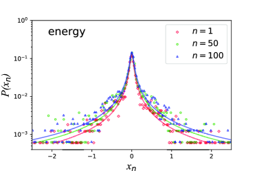
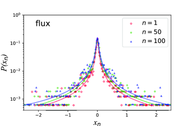
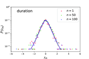
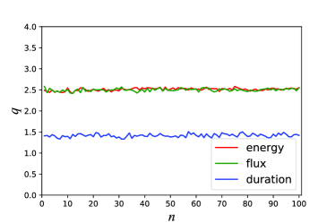
Figure 3: Scale-invariant structure of FRB 121102. PDFs of the differences of energies (upper-left panel), fluxes (upper-right panel) and durations (lower-left panel) for $n=1$ (red diamonds), $n=50$ (green circles), and $n=100$ (blue triangles), and the best-fitting $q$-Gaussian distributions (solid lines). Lower-right panel: the best-fitting $q$ values in the $q$-Gaussian distribution as a function of $n$.

Figure 3 exhibits some examples of the fits for the sample of FRB 121102. In this figure, we show the PDFs of the differences of energies (upper-left panel), fluxes (upper-right panel), and durations (lower-left panel) for $n=1$ (diamonds), $n=50$ (circles), and $n=100$ (triangles). The solid curves stand for the best-fitting results. One can see that the PDFs can be well fitted by the $q$-Gaussian function, in good agreement with the results of Lin & Sang (2020). Similar to the scenario of SGRs, we also find that the $q$-Gaussian function gives a poor fit to the PDF of the FRB waiting time differences, which is then not shown in the figure (see also Lin & Sang 2020). To better represent the scale-invariant property in FRB 121102, in the lower-right panel of Figure 3 we plot the best-fitting $q$ values as a function of the temporal interval scale $n$. We confirm that the $q$ values are almost stable and independent of $n$. This implies that there are similar scale-invariant properties among earthquakes, SGRs, and FRBs. We also list the average $q$ values of energy ($2.51\pm 0.03$), flux ($2.50\pm 0.03$), and duration ($1.42\pm 0.04$) for FRB 121102 in Table 1. We emphasize that the $q$-Gaussian distribution is a generalization of the standard Gaussian distribution and it reduces to a Gaussian distribution when $q\rightarrow 1$. Since the average $q$ value of duration is relatively small (closing to $1$), the peak of the PDF in the lower-left panel of Figure 3 is no longer very sharp as other PDFs.

4 Scale-invariant Structures of the Bimodal Energy Distribution of FRB 121102 Bursts

The burst energy distribution of FRB 121102 can be adequately described as bimodal (Li et al., 2021b). At the low energy end ($\sim E<2\times 10^{38}$ erg), a log-normal function can describe the distribution reasonably well. While the distribution at the high energy end ($\sim E>2\times 10^{38}$ erg) can be well fitted by a generalized Cauchy function. It is interesting to investigate whether low-energy bursts and high-energy bursts of FRB 121102 have a similar scale-invariant behavior.

4.1 Statistical properties of low- and high-energy bursts

We divide the overall 1652 bursts into two components, i.e., 1253 low-energy bursts with $E\leq 2\times 10^{38}$ erg and 399 high-energy bursts with $E>2\times 10^{38}$ erg. Then the scale-invariant structures of the two components are investigated, respectively. As shown in Table 1, the average $q$ values of energy, peak flux, and duration for the low-energy component are $q_{E}=1.63\pm 0.09$, $q_{P}=1.81\pm 0.05$, and $q_{T}=1.39\pm 0.06$. The average $q$ values for the high-energy component are $q_{E}=2.21\pm 0.10$, $q_{P}=2.34\pm 0.09$, and $q_{T}=1.50\pm 0.16$. Interestingly, the average $q$ value obtained from the PDFs of the energy differences of low-energy bursts is compatible, within the standard deviations, to that one found from earthquakes ($q=1.75\pm 0.15$; Caruso et al. 2007). Consistent with theoretical models of FRBs based on magnetar (e.g., Popov & Postnov 2010; Lyubarsky 2014; Beloborodov 2017, 2020; Metzger et al. 2019), the earthquake-like behavior here may indicate that the low-energy bursts of FRB 121102 could originate from starquakes of a magnetar. More interestingly, the average $q$ values of energy, peak flux, and duration for the high-energy component of FRB 121102 are roughly consistent with those of SGRs. We next show that these $q$ values can be well understood within the same statistical framework of a SOC system.

4.2 Predictions of the fractal-diffusive avalanche model

For a fractal-diffusive avalanche model, quantitative values for the size distributions of SOC parameters (length scales $L$, durations $T$, peak fluxes $P$, and fluences or energies $E$) are derived from first principles, using the scale-free probability conjecture, $N(L)dL\propto L^{-S}dL$, for three Euclidean dimensions $S=1$, 2, and 3. The analytical model predicts the indices of size distributions for $E$, $T$, and $P$ as (Aschwanden, 2012, 2014)

$$\alpha_{E} = 1+(S-1)/(D_{S}+2)$$

$$\alpha_{T} = (1+S)/2\;,$$ (5)

$$\alpha_{P} = 2-1/S$$

where $D_{S}\approx(1+S)/2$ is the mean fractal dimension. As mentioned above, Caruso et al. (2007) presented an analysis method to explain SOC behavior in the limited number of earthquakes by making use of the return distributions (i.e., distributions of the avalanche size differences at different times). They obtained the first strong evidence that the return distributions appear to have the shape of $q$-Gaussians, standard distributions arising naturally in nonextensive statistical mechanics (Tsallis, 1988; Tsallis et al., 1998). Under the assumption that there is no correlation between the sizes of two events, an exact relation between the index $\alpha$ of the avalanche size distribution and the $q$ values of the appropriate $q$-Gaussian has been obtained as (Caruso et al., 2007; Celikoglu et al., 2010)

$$q=\frac{\alpha+2}{\alpha}\;,$$ (6)

which is important because it makes the $q$ parameter determined a priori from one of the well-known indices of the system.

In the framework of the fractal-diffusive SOC model, we obtain the theoretical $q$ values, i.e., $q_{E}\approx 2.33$, $q_{P}=2.2$, and $q_{T}=2.0$, according to Equations (4.2) and (6) by taking the three-dimensional Euclidean space $S=3$. The observed $q$ values of SGR J1550–5418, SGR 1806–20, and SGR J1935+2154 at $1\sigma$ confidence level are in the range of $q_{E}\approx 2.12-2.90$, $q_{P}\approx 2.10-2.70$, and $q_{T}\approx 1.83-2.53$, which agree well with the predictions of the fractal-diffusive SOC model. We also note that the derived $q_{E}$ and $q_{P}$ of the high-energy component of FRB 121102 ($q_{E}=2.21\pm 0.10$ and $q_{P}=2.34\pm 0.09$) are in good agreement with the predictions of the fractal-diffusive SOC model, and the derived $q_{T}$ ($1.50\pm 0.16$) is also roughly consistent with the model prediction at $3.1\sigma$ confidence level. Therefore, SGRs and high-energy bursts of FRB 121102 share similar scale-invariant behavior, suggesting that they can be explained within the same statistical framework of fractal-diffusive SOC systems with the spatial dimension $S=3$.

The observed durations of the repeating bursts of FRB 121102 are directly used for the analysis of scale invariance. As is well known, the observed pulse duration of an FRB is generally broadened by the instrumental and astrophysical sources (Cordes & McLaughlin, 2003). The instrumental pulse broadening includes the sampling time-scale and the intrachannel dispersion smearing. The temporal resolution can not be better than the sampling time-scale, which broadens the pulse. The smearing is caused by intrachannel dispersion. The astrophysical pulse broadening is the scattering process of the radio emission in inhomogeneous plasma. Therefore, the observed duration does not directly represent the intrinsic duration. The intrinsic durations of the repeating bursts, in principle, should be used for our purpose. In practice, it is difficult to separate the intrinsic duration from the broadening components. But note that the distribution of the observed duration differences at different time intervals is studied in this work. Pulse broadening caused by smearing and scattering can be approximately deducted from subtracting two observed durations. That is, the difference between two observed durations can be approximated as the difference between two intrinsic ones.

5 Summary and Discussion

Previous studies have shown that the PDFs for the earthquake energy differences at different time intervals have fat tails with a $q$-Gaussian shape (Caruso et al., 2007; Wang et al., 2015). Another remarkable feature is that the $q$ values in the $q$-Gaussian distributions are approximately equal and independent of the temporal interval scale adopted, indicating a scale-invariant structure in the energy differences of earthquakes. These statistical features can be well explained within a dissipative SOC scenario taking into account long-range interactions (Caruso et al., 2007). That is, scale invariance is an important character representing the system approaching to a critical state. Recently, Chang et al. (2017) found that SGR J1550–5418 also has the property of scale invariance. However, it is unclear whether other SGRs share the same scale-invariant structure as SGR J1550–5418.

In this work, we present statistics of soft gamma-/hard X-ray bursts from SGR 1806–20 and SGR J1935+2154. We find that the two SGRs share a common behavior in terms of the PDFs of the fluence differences, confirming the findings of Chang et al. (2017). The PDFs of the fluence differences can be well fitted by a $q$-Gaussian function and the $q$ values keep nearly constant for different scale intervals. These results support that there is a common scale-invariant structure in SGRs and that systems responsible for SGR bursts are in a SOC state. Moreover, we show that the burst fluxes and durations of SGRs share similar scale-invariant behaviors with fluences, i.e., the PDFs of the differences of fluxes and durations at different time intervals also well follow $q$-Gaussian distributions.

Given the association between an FRB-like event and an X-ray burst from the Galactic magnetar SGR J1935+2154, we also investigate the scale-invariant structure of the repeating FRB 121102. For FRB 121102, we show that the PDFs of the differences of energies, fluxes, and durations also exhibit $q$-Gaussian distributions, with steady $q$ values independent of the time scale. These properties are very similar to those of SGRs, and thus both can be attributed to a SOC process. Due to the fact that the burst energy distribution of FRB 121102 is bimodal, we also investigate the scale-invariant behaviors of low- and high-energy bursts of FRB 121102. We find that the $q_{E}$, $q_{P}$, and $q_{T}$ values of low-energy bursts are different from those of high-energy bursts, which indicate that the low-energy component and the high-energy component may have different physical origins. Interestingly, the average $q$ value obtained from the PDFs of the energy differences of low-energy bursts is close to the $q$ value found from earthquakes. This implies that there may be some similarities between the energy origins of low-energy bursts of FRB 121102 and earthquakes. More interestingly, the average $q$ values of energy, peak flux, and duration for the high-energy component of FRB 121102 are roughly consistent with those of SGRs. These $q$ values can be well explained within the same statistical framework of fractal-diffusive SOC systems with the spatial dimension $S=3$. In the future, much more repeating bursts of FRBs will be detected. The physical connection between repeating FRBs and SGRs can be further investigated.

References

- Aschwanden (2011) Aschwanden, M. J. 2011, Self-Organized Criticality in Astrophysics
- Aschwanden (2012) —. 2012, A&A, 539, A2
- Aschwanden (2014) —. 2014, ApJ, 782, 54
- Aschwanden (2015) —. 2015, ApJ, 814, 19
- Aschwanden et al. (2016) Aschwanden, M. J., Crosby, N. B., Dimitropoulou, M., et al. 2016, Space Sci. Rev., 198, 47
- Bak et al. (1987) Bak, P., Tang, C., & Wiesenfeld, K. 1987, Phys. Rev. Lett., 59, 381
- Beloborodov (2017) Beloborodov, A. M. 2017, ApJ, 843, L26
- Beloborodov (2020) —. 2020, ApJ, 896, 142
- Bochenek et al. (2020) Bochenek, C. D., Ravi, V., Belov, K. V., et al. 2020, Nature, 587, 59
- Caruso et al. (2007) Caruso, F., Pluchino, A., Latora, V., Vinciguerra, S., & Rapisarda, A. 2007, Phys. Rev. E, 75, 055101
- Celikoglu et al. (2010) Celikoglu, A., Tirnakli, U., & Queirós, S. M. D. 2010, Phys. Rev. E, 82, 021124
- Chang et al. (2017) Chang, Z., Lin, H.-N., Sang, Y., & Wang, P. 2017, Chinese Physics C, 41, 065104
- Cheng et al. (1996) Cheng, B., Epstein, R. I., Guyer, R. A., & Young, A. C. 1996, Nature, 382, 518
- Cheng et al. (2020) Cheng, Y., Zhang, G. Q., & Wang, F. Y. 2020, MNRAS, 491, 1498
- CHIME/FRB Collaboration et al. (2019) CHIME/FRB Collaboration, Andersen, B. C., Bandura, K., et al. 2019, ApJ, 885, L24
- CHIME/FRB Collaboration et al. (2020) CHIME/FRB Collaboration, Andersen, B. C., Bandura, K. M., et al. 2020, Nature, 587, 54
- Cordes & Chatterjee (2019) Cordes, J. M., & Chatterjee, S. 2019, ARA&A, 57, 417
- Cordes & McLaughlin (2003) Cordes, J. M., & McLaughlin, M. A. 2003, ApJ, 596, 1142
- Duncan & Thompson (1992) Duncan, R. C., & Thompson, C. 1992, ApJ, 392, L9
- Fonseca et al. (2020) Fonseca, E., Andersen, B. C., Bhardwaj, M., et al. 2020, ApJ, 891, L6
- Foreman-Mackey et al. (2013) Foreman-Mackey, D., Hogg, D. W., Lang, D., & Goodman, J. 2013, PASP, 125, 306
- Freedman & Diaconis (1981) Freedman, D., & Diaconis, P. 1981, Probability Theory and Related Fields, 57, 453
- Geng et al. (2021) Geng, J.-J., Li, B., & Huang, Y.-F. 2021, The Innovation, 2, 100152
- Göǧüş et al. (2001) Göǧüş, E., Kouveliotou, C., Woods, P. M., et al. 2001, ApJ, 558, 228
- Göǧüş et al. (1999) Göǧüş, E., Woods, P. M., Kouveliotou, C., et al. 1999, ApJ, 526, L93
- Göǧüş et al. (2000) —. 2000, ApJ, 532, L121
- Hurley et al. (1999) Hurley, K., Cline, T., Mazets, E., et al. 1999, Nature, 397, 41
- Kaspi & Beloborodov (2017) Kaspi, V. M., & Beloborodov, A. M. 2017, ARA&A, 55, 261
- Katz (1986) Katz, J. I. 1986, J. Geophys. Res., 91, 10,412
- Katz (2016) —. 2016, ApJ, 826, 226
- Kırmızıbayrak et al. (2017) Kırmızıbayrak, D., Şaşmaz Muş, S., Kaneko, Y., & Göğüş, E. 2017, ApJS, 232, 17
- Kouveliotou et al. (1998) Kouveliotou, C., Dieters, S., Strohmayer, T., et al. 1998, Nature, 393, 235
- Kulkarni et al. (2014) Kulkarni, S. R., Ofek, E. O., Neill, J. D., Zheng, Z., & Juric, M. 2014, ApJ, 797, 70
- Kumar et al. (2017) Kumar, P., Lu, W., & Bhattacharya, M. 2017, MNRAS, 468, 2726
- Li et al. (2021a) Li, C. K., Lin, L., Xiong, S. L., et al. 2021a, Nature Astronomy, 5, 378
- Li et al. (2018) Li, D., Wang, P., Qian, L., et al. 2018, IEEE Microwave Magazine, 19, 112
- Li et al. (2021b) Li, D., Wang, P., Zhu, W. W., et al. 2021b, arXiv e-prints, arXiv:2107.08205
- Lin & Sang (2020) Lin, H.-N., & Sang, Y. 2020, MNRAS, 491, 2156
- Lin et al. (2020a) Lin, L., Göğüş, E., Roberts, O. J., et al. 2020a, ApJ, 902, L43
- Lin et al. (2020b) —. 2020b, ApJ, 893, 156
- Lorimer et al. (2007) Lorimer, D. R., Bailes, M., McLaughlin, M. A., Narkevic, D. J., & Crawford, F. 2007, Science, 318, 777
- Lyu et al. (2020) Lyu, F., Li, Y.-P., Hou, S.-J., et al. 2020, Frontiers of Physics, 16, 14501
- Lyu et al. (2021) Lyu, F., Meng, Y.-Z., Tang, Z.-F., et al. 2021, Frontiers of Physics, 16, 24503
- Lyubarsky (2014) Lyubarsky, Y. 2014, MNRAS, 442, L9
- Lyutikov (2003) Lyutikov, M. 2003, MNRAS, 346, 540
- Mazets et al. (1979) Mazets, E. P., Golentskii, S. V., Ilinskii, V. N., Aptekar, R. L., & Guryan, I. A. 1979, Nature, 282, 587
- Mereghetti et al. (2020) Mereghetti, S., Savchenko, V., Ferrigno, C., et al. 2020, ApJ, 898, L29
- Metzger et al. (2017) Metzger, B. D., Berger, E., & Margalit, B. 2017, ApJ, 841, 14
- Metzger et al. (2019) Metzger, B. D., Margalit, B., & Sironi, L. 2019, MNRAS, 485, 4091
- Murase et al. (2016) Murase, K., Kashiyama, K., & Mészáros, P. 2016, MNRAS, 461, 1498
- Nan et al. (2011) Nan, R., Li, D., Jin, C., et al. 2011, International Journal of Modern Physics D, 20, 989
- Olami et al. (1992) Olami, Z., Feder, H. J. S., & Christensen, K. 1992, Phys. Rev. Lett., 68, 1244
- Olausen & Kaspi (2014) Olausen, S. A., & Kaspi, V. M. 2014, ApJS, 212, 6
- Palmer et al. (2005) Palmer, D. M., Barthelmy, S., Gehrels, N., et al. 2005, Nature, 434, 1107
- Petroff et al. (2019) Petroff, E., Hessels, J. W. T., & Lorimer, D. R. 2019, A&A Rev., 27, 4
- Platts et al. (2019) Platts, E., Weltman, A., Walters, A., et al. 2019, Phys. Rep., 821, 1
- Popov & Postnov (2010) Popov, S. B., & Postnov, K. A. 2010, in Evolution of Cosmic Objects through their Physical Activity, ed. H. A. Harutyunian, A. M. Mickaelian, & Y. Terzian, 129–132
- Prieskorn & Kaaret (2012) Prieskorn, Z., & Kaaret, P. 2012, ApJ, 755, 1
- Ridnaia et al. (2021) Ridnaia, A., Svinkin, D., Frederiks, D., et al. 2021, Nature Astronomy, 5, 372
- Spitler et al. (2016) Spitler, L. G., Scholz, P., Hessels, J. W. T., et al. 2016, Nature, 531, 202
- Tavani et al. (2021) Tavani, M., Casentini, C., Ursi, A., et al. 2021, Nature Astronomy, 5, 401
- The CHIME/FRB Collaboration et al. (2021) The CHIME/FRB Collaboration, :, Amiri, M., et al. 2021, arXiv e-prints, arXiv:2106.04352
- Thompson & Duncan (1995) Thompson, C., & Duncan, R. C. 1995, MNRAS, 275, 255
- Tsallis (1988) Tsallis, C. 1988, Journal of Statistical Physics, 52, 479
- Tsallis et al. (1998) Tsallis, C., Mendes, R., & Plastino, A. R. 1998, Physica A Statistical Mechanics and its Applications, 261, 534
- Turolla et al. (2015) Turolla, R., Zane, S., & Watts, A. L. 2015, Reports on Progress in Physics, 78, 116901
- Wadiasingh & Timokhin (2019) Wadiasingh, Z., & Timokhin, A. 2019, ApJ, 879, 4
- Wang & Dai (2013) Wang, F. Y., & Dai, Z. G. 2013, Nature Physics, 9, 465
- Wang et al. (2020) Wang, F. Y., Wang, Y. Y., Yang, Y.-P., et al. 2020, ApJ, 891, 72
- Wang & Yu (2017) Wang, F. Y., & Yu, H. 2017, J. Cosmology Astropart. Phys, 2017, 023
- Wang et al. (2015) Wang, P., Chang, Z., Wang, H., & Lu, H. 2015, European Physical Journal B, 88, 206
- Xiao et al. (2021) Xiao, D., Wang, F., & Dai, Z. 2021, Science China Physics, Mechanics, and Astronomy, 64, 249501
- Yang & Zhang (2018) Yang, Y.-P., & Zhang, B. 2018, ApJ, 868, 31
- Zhang (2020) Zhang, B. 2020, Nature, 587, 45
- Zhang et al. (2018) Zhang, Y. G., Gajjar, V., Foster, G., et al. 2018, ApJ, 866, 149