Image Scene Graph Generation (SGG) Benchmark

Abstract

There is a surge of interest in image scene graph generation (object, attribute and relationship detection) due to the need of building fine-grained image understanding models that go beyond object detection. Due to the lack of a good benchmark, the reported results of different scene graph generation models are not directly comparable, impeding the research progress. We have developed a much-needed scene graph generation benchmark based on the maskrcnn-benchmark[13] and several popular models. This paper presents main features of our benchmark and a comprehensive ablation study of scene graph generation models using the Visual Genome[11] and OpenImages Visual relationship detection[10] datasets. Our codebase is made publicly available at https://github.com/microsoft/scene_graph_benchmark.

1 Introduction

Understanding a visual scene goes beyond recognizing individual objects in isolation. Visual attributes of an object and relationships between objects also constitute rich semantic information about the scene. Scene Graph Generation (SGG) [18] is a task to detect objects, their attributes and relationships using scene graphs [11], a visually-grounded graphical structure of an image. SGG has proven useful for building more visually-grounded and compositional models for other computer vision and vision-language tasks, like image/text retrieval [9, 17], image captioning [4, 20, 6], visual question answering [3, 5], action recognition [7], image generation [8, 14], and 3D scene understanding [2].

Code base	Supported datasets	Supported methods	Last commit time (Pytorch version)	Attribute detection	OD/SGG decouple-able
Neural Motif [21]	VG	IMP,NM	11/07/2018 (0.3)	No	No
RelDN [22]	VG, OI	NM,GRCNN,RelDN	08/19/2019 (1.0)	No	Yes
GRCNN [19]	VG	IMP,MSDN,GRCNN	03/31/2020 (1.0)	No	No
SGG-Pytorch [15]	VG	IMP,NM,VCTree [16]	12/13/2020 (1.2)	Yes	No
SG Benchmark (ours)	VG, OI	IMP,MSDN,NM,GRCNN,RelDN	06/07/2021 (1.7)	Yes	Yes

Table 1: Comparison of different open-sourced code bases for scene graph generation (SGG). Our code base supports two datasets (Visual Genome (VG) and Open Images (OI)) and five popular SGG methods. It is maintained regularly with up-to-date Pytorch support. It supports both attribute and relationship detection, and its object detection module (OD) and SGG module are decouple-able, which enables user to use customized OD models/results.

There are several open-sourced code bases and models for SGG, see, e.g., [21, 19, 22, 15]. However, none of the existing code bases satisfies the following five criteria that from our perspective are important for easy use: (1) Support both Visual Genome (VG) and Open Images (OI) datasets, where VG is a popular academic testbed and OI is a large-scale public benchmark; (2) Support various popular methods, especially RelDN [22] that we found is very effective in improving SGG performance; (3) Under continuous maintenance and up-to-date Pytorch support; (4) Support attribute detection, which is crucial in vision-language downstream tasks [1, 23]; and (5) Make the object detection (OD) module and the SGG module decouple-able, allowing users to use their customized detection models and results. Our SGG Benchmark code base, built on top of maskrcnn-benchmark [13], satisfies all these five criteria and has several other useful features. We compare ours with existing SGG code bases in Table 1 and list main features of our code base as below.

• Provide a generic SGG dataset class that supports both VG and OI datasets and is easily adaptable to customized SGG datasets. We have integrated evaluation metrics from official Open Images relationship detection challenge for OpenImages Visual relationship detection[10], and implemented widely used Visual Genome relationship detection Recall calculation for scene graph generation on the Visual Genome[11].

• Support multiple popular scene graph generation algorithms. We have integrated five widely used scene graph generation algorithms into our framework, including iterated message passing (IMP) [18], multi-level scene detection networks (MSDN) [12], graph R-CNN (GRCNN) [19], neural motif (NM) [21] and RelDN [22].

• Modular design with decouple-able object detection and SGG modules. We have decomposed SGG framework into three components: object detection, attribute classification and relationship detection. One can easily replace or insert new components. Our framework decouples object detection and relationship detection so that one can do relationship detection with bounding boxes and labels from any object detector.

• Fast and portable dataset format. Our code base uses Tab Separated Values (TSV) data format, which is portable and flexible for data manipulations. We have also developed tools to visualize this data format directly. We will release the visualization tool later.

• Large models with state of the art performance. We have trained large models with ResNeXt-152 backbone for both object detection and scene graph generation. Our large models achieve state of the art performance on both Open Images relationship detection and Visual Genome scene graph generation.

• Image feature extraction for downstream vision-language tasks. We provide a easy-to-use pipeline to extract object and relation features from our pretrained models. The features exacted from our large models, when used as the input of downstream vision-language models, achieve SOTA performance on seven major vision-language tasks [23].

Besides presenting major improvements in our code base (Section 2) and benchmarking results on VG and OI datasets (Section 3), we report a comprehensive ablation study of current models’ capability in Section 4. We study the frequency prior in relationship detection and found that the SOTA models are only slightly better than the frequency prior baseline. We also ablate the error of SGG models into different sources, including object detection error, relation proposal error and relation classification error. We hope the study can provide insights to build better SGG models.

2 Major improvements in SGG methods.

In our code base, we have re-implemented five widely used SGG algorithms, i.e, IMP [18], MSDN [12], GRCNN [19], NM [21] and RelDN [22], with two major improvements as described below.

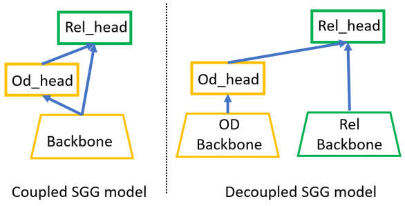
Figure 1: Illustration of coupled and decoupled SGG model architecture.

2.1 Decouple object and relationship detection

Most existing SGG models use a two-stage model architecture (object detection first and then relationship prediction), e.g., [18, 12, 19, 21], where the relationship detection module extracts relation features from the same backbone of the object detection module, as shown in Figure 1 Left. The object detector (the yellow part) is pre-trained with the object detection task. To train the relationship detection module (the green part), one either (1) trains only the parameters in the relationship detection module, resulting in sub-optimal relationship detection performance, or (2) trains the full network with both object and relationship detection losses in a multi-task learning fashion, typically resulting in OD performance drop compared to the pre-trained object detector. This tightly coupled model architecture also makes SGG models difficult to make use of off-the-shelf object detectors, such as calling a Cloud service for object detection.

To resolve these issues, our code base supports both the coupled and decoupled SGG model architecture. As shown in Figure 1 Right, the decoupled model introduces a separate relation backbone for relationship detection, which enables users to use their customized detection models/results. In our current implementation, we use [13] as our object detector, but the decoupled model can receive detection results from any object detectors. In Table 5, we show that this decoupled model architecture outperforms the coupled counterpart. The extra computational and memory cost from the relation backbone is minor, because the major cost of an SGG model is from its relation head.

2.2 No refinement of object detection results

It is a common practice in training SGG models that the relationship detection module also learns to output refined object detection results, which either only refines the object classification (labels and confidences), e.g., [18, 12, 19], or refines both object classification and box regression, e.g., [21]. This refinement introduces extra OD parameters and an OD loss in the relationship detection module. The hope is that by jointly training OD and relationship detection, the OD performance can be improved. However, we found that it is not the case. The refined OD results are typically worse than the pre-trained OD results. As shown in Table 6, the worse and constantly-changing OD results also make it more difficult to train the relationship module, resulting in worse relationship detection performance. Therefore, we do not refine the object detection results in the relationship module.

3 SGG Benchmarks on VG and OI

3.1 Datasets and evaluation metrics

Our code base provides a generic SGG dataset class that supports both VG and OI datasets. It is easily adaptable to customized SGG datasets, too. We listed the main features of these two datasets and their evaluation metrics as below.

Visual Genome Scene Graph Generation. The Visual Genome dataset for Scene Graph Generation, introduced by IMP [18], contains 150 object and 50 relation categories. We follow their train/val splits. The evaluation codes are adopted from IMP [18] and NM [21]. The evaluation metrics are based on Recalls of three settings: (1) predicate classification (predcls): given a ground truth set of object boxes and labels, predict edge labels, (2) scene graph classification (sgcls): given ground truth boxes, predict box labels and edge labels and (3) scene graph detection (sgdet): predict boxes, box labels and edge labels.

Open Images Visual Relationship Detection. We follow Open Images Challenge 2018 Visual Relationship Detection Track. We use official recommended validation subset to split the data. The train and val sets contains 53,953 and 3,234 images respectively. There are 9 different relationships, 57 different object classes and 5 different attributes. We adopt the evaluation code from Open Images Visual Relationship Detection Challenge 2018 official evaluation. The metrics are based on detection average precision/recall. Following RelDN, we scale each predicate category by their relative ratios in the val set, which we refer to as the weighted mAP (wmAP), to solve extreme predicate class imbalance problem. The final evaluation score is calculated as $Score=0.2*recall@50+0.4*wmAP(Triplet)+0.4*wmAP(Phrase)$.

3.2 SGG methods and frequency baselines

We benchmark five scene graph generation methods, including iterative message passing (IMP) [18], multi-level scene detection networks (MSDN) [12], graph R-CNN (GRCNN) [19], Neural Motif [21] and RelDN [22].

Since object labels are highly predictive of relationship labels, we additionally include two simple yet strong frequency baselines (first proposed in [21]) built from training set statistics. The first, “Freq”, gives the most likely relation type given the object and subject labels, based on training set statistics. The second, “Freq+Overlap”, additionally requires that the two boxes have overlap in order for the pair to count as a valid relation.

3.3 Benchmarking Results

We present benchmarking results on Open Images Visual Relationship Detection in Table 2. The object detection model is a ResNeXt152-FPN detector trained on OpenImagesVRD dataset. Its performance is 76.11 mAP@0.5 over 57 object classes used in relation detection. The RelDN performs the best. The “Freq+Overlap” baseline performs very competitively, better or as good as all methods except RelDN. Thanks to the large and strong ResNeXt152 backbone, our new RelDN result sets a new SOTA performance on this OI VRD task.

Model	Score	Recall@50	wmAP(Triplet)	mAP(Triplet)	wmAP(Phrase)	mAP(Phrase)	Triplet proposal recall	Phrase proposal recall
Neural Motif	39.48	72.54	29.35	29.26	33.10	35.02	73.64	78.70
MSDN	39.64	71.76	30.40	36.76	32.81	40.89	72.54	75.85
IMP	40.01	71.81	30.88	45.97	33.25	50.42	72.81	76.04
Freq+Overlap	40.12	72.63	30.18	31.82	33.81	37.08	74.81	78.26
GRCNN	43.54	74.17	34.73	39.56	37.04	43.63	74.11	77.32
RelDN	51.08	75.40	40.85	44.24	49.16	50.60	78.74	90.39

Table 2: Open Images Scene Graph Detection results on val set. All models share the same object detector, which is an ResNeXt152-FPN detector trained on 57 object classes used in this dataset. All models are inferenced in unconstrained mode (each subject and object pair can have at most 2 predicates).

We present benchmarking results on Visual Genome in Table 3. The object detection model is a ResNet50-FPN detector trained on Visucal Genome. Its performance is 28.15 mAP@0.5 over 150 object classes. RelDN is still the best performer. All the other methods achieve similar performance as the “Freq+Overlap” baseline.

Model	sgdet@20	sgdet@50	sgdet@100	sgcls@20	sgcls@50	sgcls@100	predcls@20	predcls@50	predcls@100
Neural Motif	21.8	30.1	33.8	30.2	35.1	36.5	52.1	61.2	63.2
Freq+Overlap	21.6	29.0	34.0	31.9	35.7	36.6	53.4	60.5	62.1
IMP	21.7	29.3	34.5	29.2	33.9	35.3	48.8	57.6	59.9
MSDN	22.4	30.0	35.3	29.7	34.4	35.9	51.2	59.6	61.6
GRCNN	22.9	30.1	34.8	30.5	34.9	36.2	52.1	59.9	61.8
RelDN	24.0	32.4	37.8	31.9	35.7	36.6	54.0	60.9	62.5

Table 3: Visual Genome Scene Graph Detection results on val set. All models share the same object detector, which is a ResNet50-FPN detector. All models are evaluated in constrained mode (each subject and object pair can only have 1 predicate).

4 Ablation Experiments

In order to justify our two major changes to existing SGG methods and understand the limitation of these methods, we perform the following ablation study on the OI VRD task.

Coupled vs decoupled SGG model architecture. As mentioned in Section 2.1, our code base supports both the coupled and decoupled model architecture. In Table 5, we show that the decoupled arch outperforms the coupled arch. Table 5 also shows that the coupled arch with full model trained by both object and relation detection losses performs the worst. This indicates that the relationship detection task is not helping object detection, but instead making its performance worse.

OD	Relation	score	Recall@50	wmAP(Triplet)	mAP(Triplet)	wmAP(Phrase)	mAP(Phrase)	Triplet proposal recall	Phrase proposal recall
predicted objects	“Freq+Overlap”	40.12	72.63	30.18	29.35	33.81	34.05	77.10	89.92
predicted objects	model relation	46.96	74.42	38.78	41.38	41.41	44.68	77.51	89.98
gt objects	“Freq+Overlap”	78.94	93.38	77.87	73.89	72.81	68.67	93.87	94.73
gt objects	model relation	86.41	93.29	86.46	85.36	82.93	81.76	93.84	97.32
gt objects	gt pairs + “Freq+Overlap”	95.58	99.89	97.21	84.72	91.80	79.66	100	100
gt objects	gt pairs + predicted relation	94.21	99.86	95.22	84.67	90.38	80.43	100	100

Table 4: We use the pre-trained RelDN model from [22] for this ablation study. The mAP of object detector (ResNeXt101-FPN) is 71.33. When using predicted bounding box, the bbox pair recall (regardless of predicate) are 86.94(Triplet) and 95.17(Phrase).

Model	Recall@50
Coupled, only Rel_head is trained	74.31
Coupled, full model is trained	66.47
Decoupled	75.40

Table 5: Comparison of coupled and decoupled models. All these experiments are conducted on OI VRD Dataset with ResNeXt152-FPN as backbone and RelDN as relation head.

Model	refined	not refined
IMP	69.90	71.43
MSDN	68.08	71.36
Neural Motif	71.46	72.68

Table 6: Comparison of using object label predicted by relation head (refined object detection) and label predicted by pre-trained object detector. All models are trained on OI VRD dataset with ResNeXt152-FPN backbone and the reported numbers are Recall@50.

Should OD be refined or not? In Table 6, we show that it is more desirable to directly use the pre-trained OD results in the relationship detection module, instead of further refining them.

Ablate SGG error into different sources. In Table 4, we ablate SGG errors into three sources: errors from object detection (predicted objects vs ground-truth objects), errors from relation proposal (model’s proposed pairs vs ground-truth pairs), and errors from relation classification. We use two models for this experiment: the pre-trained RelDN model (ResNeXt101-FPN) from [22] and the “Freq+Overlap” baseline. We can see that the majority of SGG error comes from the object detection, because the score jumps from 40.96 to 86.41 by replacing the predicted objects with the ground-truth objects. The relation proposal is the second major source of SGG error source, because the score jumps from 86.41 to 94.21 by further replacing the proposed pairs with the ground-truth pairs. Finally, the classification error contributes to the gap from 94.21 to 100. Table 4 also shows that the “Freq+Overlap” baseline is even better than the RelDN model in terms of relation classification, but worse in terms of relation proposals.

The barrier of frequency/language prior. As discussed in the last paragraph, the models’ relation classification capability is almost the same as the ”Freq+Overlap” baseline on OI VRD. Since VG task has more predicate classes (50) compared with OI VRD (10), it would be more difficult for the ”Freq+Overlap” baseline. Therefore, we use models trained on VG task to further study if SGG methods only learned the frequency prior from training data. In Table 7, we first compute every method’s relation classification accuracy (the diagonal part) and their pair-wise perfect ensemble accuracy (the lower-diagonal part). As the diagonal shows, all the methods has nearly the same and are slightly worse than the ”Freq+Overlap” baseline. However, all the methods are to some degree different from the ”Freq+Overlap” baseline because the pair-wise ensemble models (the last row) are clearly better than those single models (the diagonal). To further quantify the similarity of two SGG models (including the ”Freq+Overlap” baseline), We calculated their pair-wise similarity based on models’ predictions in Table 8. From these results, we can see the model predictions similarity range from 70.89% to 84.17%. From these results, we conclude that the difference in terms of relation classification capability between learned SGG models and the ”Freq+Overlap” baseline are very small. To further improve SGG performance, new SGG methods should learn more visual signals different from the frequency prior.

Model	IMP	MSDN	Neural Motif	GRCNN	RelDN	Freq+Overlap
IMP	63.85
MSDN	69.85	64.82
Neural Motif	67.71	70.27	65.21
GRCNN	70.61	68.51	70.57	64.80
RelDN	71.14	70.03	70.67	69.99	66.12
Freq+Overlap	70.38	69.36	69.69	69.76	69.03	66.23

Table 7: Visual Genome models predicate predictions pair-wise ensemble accuracy ($\frac{TP+TN}{TP+TN+FP+FN}$). We assume a perfect ensemble setting where the ensemble model is correct as long as there is a correct prediction in the ensemble.

Model	IMP	MSDN	Neural Motif	GRCNN	RelDN	Freq+Overlap
IMP	100
MSDN	73.83	100
Neural Motif	84.17	74.53	100
GRCNN	71.06	80.12	73.59	100
RelDN	70.89	75.98	75.15	76.86	100
Freq+Overlap	74.49	79.17	80.30	78.21	83.56	100

Table 8: Visual Genome model predictions similarity comparison under force relation mode. The similarity is defined as $\frac{\text{\# matched triplets}}{\text{\# total unique triplets}}$, triplet is defined as $(subj\_instance,predicate,obj\_instance)$.

5 Feature Extraction Pipelines

Our SGG benchmark supports feature extraction for downstream computer vision and vision-language tasks. Given an image, we can extract both object-level features and relation-level features.

Object-level features are extracted from the object detector. Each bounding box has a feature vector. Relation-level features are extracted from the scene graph detector. Each relation pair has a feature vector.

References

- [1] P. Anderson, X. He, C. Buehler, D. Teney, M. Johnson, S. Gould, and L. Zhang. Bottom-up and top-down attention for image captioning and visual question answering. In CVPR, 2018.
- [2] I. Armeni, Z.-Y. He, J. Gwak, A. R. Zamir, M. Fischer, J. Malik, and S. Savarese. 3d scene graph: A structure for unified semantics, 3d space, and camera. In Proceedings of the IEEE/CVF International Conference on Computer Vision, pages 5664–5673, 2019.
- [3] H. Ben-Younes, R. Cadene, N. Thome, and M. Cord. Block: Bilinear superdiagonal fusion for visual question answering and visual relationship detection. In Proceedings of the AAAI Conference on Artificial Intelligence, volume 33, pages 8102–8109, 2019.
- [4] L. Gao, B. Wang, and W. Wang. Image captioning with scene-graph based semantic concepts. In Proceedings of the 2018 10th International Conference on Machine Learning and Computing, pages 225–229, 2018.
- [5] S. Ghosh, G. Burachas, A. Ray, and A. Ziskind. Generating natural language explanations for visual question answering using scene graphs and visual attention. arXiv preprint arXiv:1902.05715, 2019.
- [6] J. Gu, S. Joty, J. Cai, H. Zhao, X. Yang, and G. Wang. Unpaired image captioning via scene graph alignments. In Proceedings of the IEEE/CVF International Conference on Computer Vision, pages 10323–10332, 2019.
- [7] J. Ji, R. Krishna, L. Fei-Fei, and J. C. Niebles. Action genome: Actions as composition of spatio-temporal scene graphs, 2019.
- [8] J. Johnson, A. Gupta, and L. Fei-Fei. Image generation from scene graphs. In Proceedings of the IEEE conference on computer vision and pattern recognition, pages 1219–1228, 2018.
- [9] J. Johnson, R. Krishna, M. Stark, L.-J. Li, D. Shamma, M. Bernstein, and L. Fei-Fei. Image retrieval using scene graphs. In Proceedings of the IEEE Conference on Computer Vision and Pattern Recognition (CVPR), June 2015.
- [10] I. Krasin, T. Duerig, N. Alldrin, V. Ferrari, S. Abu-El-Haija, A. Kuznetsova, H. Rom, J. Uijlings, S. Popov, S. Kamali, M. Malloci, J. Pont-Tuset, A. Veit, S. Belongie, V. Gomes, A. Gupta, C. Sun, G. Chechik, D. Cai, Z. Feng, D. Narayanan, and K. Murphy. Openimages: A public dataset for large-scale multi-label and multi-class image classification. Dataset available from https://storage.googleapis.com/openimages/web/index.html, 2017.
- [11] R. Krishna, Y. Zhu, O. Groth, J. Johnson, K. Hata, J. Kravitz, S. Chen, Y. Kalantidis, L.-J. Li, D. A. Shamma, M. Bernstein, and L. Fei-Fei. Visual genome: Connecting language and vision using crowdsourced dense image annotations. 2016.
- [12] Y. Li, W. Ouyang, B. Zhou, K. Wang, and X. Wang. Scene graph generation from objects, phrases and region captions. 2017 IEEE International Conference on Computer Vision (ICCV), Oct 2017.
- [13] F. Massa and R. Girshick. maskrcnn-benchmark: Fast, modular reference implementation of Instance Segmentation and Object Detection algorithms in PyTorch. https://github.com/facebookresearch/maskrcnn-benchmark, 2018. Accessed: [Insert date here].
- [14] T. Sylvain, P. Zhang, Y. Bengio, R. D. Hjelm, and S. Sharma. Object-centric image generation from layouts, 2020.
- [15] K. Tang. A scene graph generation codebase in pytorch, 2020. https://github.com/KaihuaTang/Scene-Graph-Benchmark.pytorch.
- [16] K. Tang, H. Zhang, B. Wu, W. Luo, and W. Liu. Learning to compose dynamic tree structures for visual contexts. In Proceedings of the IEEE/CVF Conference on Computer Vision and Pattern Recognition, pages 6619–6628, 2019.
- [17] S. Wang, R. Wang, Z. Yao, S. Shan, and X. Chen. Cross-modal scene graph matching for relationship-aware image-text retrieval. In Proceedings of the IEEE/CVF Winter Conference on Applications of Computer Vision, pages 1508–1517, 2020.
- [18] D. Xu, Y. Zhu, C. B. Choy, and L. Fei-Fei. Scene graph generation by iterative message passing. 2017 IEEE Conference on Computer Vision and Pattern Recognition (CVPR), Jul 2017.
- [19] J. Yang, J. Lu, S. Lee, D. Batra, and D. Parikh. Graph r-cnn for scene graph generation. Lecture Notes in Computer Science, page 690–706, 2018.
- [20] X. Yang, K. Tang, H. Zhang, and J. Cai. Auto-encoding scene graphs for image captioning. In Proceedings of the IEEE/CVF Conference on Computer Vision and Pattern Recognition, pages 10685–10694, 2019.
- [21] R. Zellers, M. Yatskar, S. Thomson, and Y. Choi. Neural motifs: Scene graph parsing with global context. 2018 IEEE/CVF Conference on Computer Vision and Pattern Recognition, Jun 2018.
- [22] J. Zhang, K. J. Shih, A. Elgammal, A. Tao, and B. Catanzaro. Graphical contrastive losses for scene graph parsing, 2019.
- [23] P. Zhang, X. Li, X. Hu, J. Yang, L. Zhang, L. Wang, Y. Choi, and J. Gao. Vinvl: Making visual representations matter in vision-language models. arXiv preprint arXiv:2101.00529, 2021.