Ultra high-energy cosmic rays from beyond the Greisen-Zatsepin-Kuz’min horizon

Abstract

Ultra-high-energy (UHE) cosmic rays (CRs) of energies $\sim(10^{18}-10^{20})~{}{\rm eV}$, accelerated in violent astrophysical environments, interact with cosmic background radiation fields via photo-hadronic processes, leading to strong attenuation. Typically, the Universe would become ‘opaque’ to UHE CRs after several tens of Mpc, setting the boundary of the Greisen-Zatsepin-Kuz’min (GZK) horizon. In this work, we investigate the contribution of sources beyond the conventional GZK horizon to the UHE CR flux observed on Earth, when photo-spallation of the heavy nuclear CRs is taken into account. We demonstrate this contribution is substantial, despite the strong attenuation of UHE CRs. A significant consequence is the emergence of an isotropic background component in the observed flux of UHE CRs, coexisting with the anisotropic foreground component that are associated with nearby sources. Multi-particle CR horizons, which evolve over redshift, are determined by the CR nuclear composition. Thus, they are dependent on the source populations and source evolutionary histories.

1 Introduction

Ultra high-energy (UHE) cosmic-ray (CR) events are rare. Although the detection of UHE CRs with energies $E>10^{20}\;\!{\rm eV}$ has been reported (e.g. Bird et al., 1994, 1995), their flux $J(E)$ at sea level, given by $E^{3}J(E)\approx 10^{24}\ {\rm{eV^{2}}\;\!m^{-2}\;\!s^{-1}\;\!sr^{-1}}$, at energy $E=10^{20}\;\!{\rm eV}$ (see e.g. Abu-Zayyad et al., 2013; Ivanov, 2017), implies an event rate of only 1 particle per square km per century. Several origins of these UHE CRs have been proposed, based on the argument that charged particles can, in principle, be accelerated to energies as high as $10^{20}\;\!{\rm eV}$ in astrophysical environments, including the relativistic jets of active galactic nuclei (AGN), the large-scale shocks associated with galaxy clusters, and neutron stars, as indicated by the Hillas (1984) criteria.

High energy CR protons and nuclei interact with photons, and these interactions lead to the generation of lower energy subatomic particles. Cosmic Microwave Background (CMB) radiation and Extra-galactic Background Light (EBL) permeate the Universe, and these provide a target for UHE CR interactions, via photo-hadronic processes. Such photo-hadronic interactions attenuate the flux of CRs at high energies, setting an energy limit above which the CR flux detected at Earth would drop very substantially. This energy is around $\sim 10^{20}\;\!{\rm eV}$ (Greisen, 1966; Zatsepin & Kuz’min, 1966) and is known as the Greisen-Zatsepin-Kuz’min (GZK) limit (For reviews of GZK limit, see e.g. Watson, 2014; Kachelrieß & Semikoz, 2019). Photo-hadronic interactions also limit the intergalactic distance over which CR protons and nuclei can travel. For instance, the expected survival distance of a CR proton of $E_{\rm p}\approx 3\times 10^{20}\;\!{\rm eV}$ traversing through a blackbody radiation field of a temperature $2.7\;\!{\rm K}$), is $<30\;\!{\rm Mpc}$ (see e.g. Kachelrieß & Semikoz, 2019). This has led to a belief that the extra-galactic UHE CR flux with $E\sim 10^{20}~{}{\rm eV}$ detected on Earth is likely comprised of CRs originating in nearby foreground sources within a horizon (hereafter, referred to as the ‘GZK horizon’) of radius $\sim 50\;\!{\rm Mpc}$, and a residual, heavily-attenuated background flux from more distant source populations.

If we accept the Hillas (1984) criteria strictly, the number of possible UHE CR sources within the GZK horizon is limited. Because of this and the close proximity of sources, if the propagation of UHE protons and nuclei is ballistic, their arrival directions as observed at Earth would not be isotropic. Instead, they would be preferentially oriented towards nearby UHE CR sources that fall within the GZK horizon. Recent studies (for reviews, see Kotera & Olinto, 2011; Deligny et al., 2017; Alves Batista et al., 2019b; Rieger, 2019) have searched for anisotropies in the arrival directions of UHE CRs (Abreu et al., 2010; Aab et al., 2014, 2015; Pierre Auger Collaboration et al., 2017; Aab et al., 2018; Abbasi et al., 2018), with Pierre Auger Collaboration et al. (2017) reporting a detection for CRs of energies above $8\times 10^{18}\;\!{\rm eV}$ at a significance $>5.2\sigma$ (see section 4.2 for further discussion). Complementary studies investigating correlations between UHE CR arrival directions and catalogues of possible sources (in particular, AGN) have also returned encouraging results (see Pierre Auger Collaboration et al., 2007; Abreu et al., 2010). However, stronger correlations result if the UHE CR flux arriving at Earth is considered to have two components: an anisotropic source component (presumably from nearby high-energy cosmic accelerators), and an isotropic background component (Kim & Kim, 2011).

In this work, we investigate the interactions of UHE CRs with the CMB and EBL, considering in particular how photo-spallation and photo-pion interactions affect the propagation and attenuation of UHE CR nuclei. We investigate how much of the UHE CR flux originates from distant sources, and assess its dependence on CR composition and source population models. We show that distant CR sources, together with secondary CRs produced by photo-spallation could supply a significant isotropic flux in the UHE CRs observed at Earth. The paper is organized as follows: in Section 2, we introduce our models for the propagation and interaction of energetic CR nuclei through intergalactic radiation fields, accounting for the relevant micro-physics and particle interactions. In Section 3, we introduce our CR source population, composition and spectral model. We present our results in Section 4 and summarize our findings and present conclusions in Section 5.

2 Cosmological interactions and propagation of cosmic rays

2.1 Ultra high-energy cosmic ray interactions

2.1.1 Protons and neutrons

Energetic protons interact with ambient radiation fields to produce leptons and pions. These photo-hadronic interactions are dominated by Bethe-Heitler (BH) photo-pair production (Bethe & Heitler, 1934) and photo-pion production processes. Photo-pair processes proceed as

$${\rm A}^{\prime}+\gamma\rightarrow{\rm A}+{l}^{+}+{l}^{-}\ ,$$ (1)

where ${\rm A}^{\prime}$ and ${\rm A}$ are nucleons before and after the interaction respectively, while ${l}^{+}$ and ${l}^{-}$ are the leptons and anti-leptons produced in this process. As photo-electron pair production contributes most to photo-pair CR energy losses (see e.g. Blumenthal, 1970; Klein, 2006) over the range of energies of interest in this work, we consider only the production of electrons (${e}^{-}$) and positrons (${e}^{+}$). Without loss of generality, hereafter we do not distinguish between electrons and positrons unless otherwise stated, and both are referred to as “electrons”.

Photo-pion production operates mostly through the following channels: (i) resonant single-pion production, (ii) direct single-pion production, and (iii) multiple-pion production (Mücke et al., 1999). Resonant single-pion production arises through the production of $\Delta^{+}$ intermediaries, which decay predominantly through the channels:

$$\rm{p}+\gamma \rightarrow\Delta^{+}\rightarrow\begin{cases}\rm{p}+\pi^{0}\rightarrow\rm{p}+2\gamma\\[2.15277pt] \rm{n}+\pi^{+}\rightarrow\rm{n}+\mu^{+}+\nu_{\mu}\\ \hskip 66.00015pt\leavevmode\hbox to11.36pt{\vbox to12.46pt{\text{[drawing]}}}~{}\rm{e}^{+}+\nu_{\rm e}+\bar{\nu}_{\mu}\end{cases}$$ (2)

(see Berezinsky & Gazizov, 1993). The decays produce charged and neutral pions, and their branching ratios (BRs) are roughly 2/3 and 1/3 respectively. The pions will further decay, producing cascades of lower-energy particles. Multi-pion production occurs at higher energies (see Mücke et al., 1999), and when the invariant interaction energy exceeds $\epsilon_{\rm r}\approx 3500$, charged and neutral pion production can arise with high multiplicities. For the energy range of interest in this work, each type of pion is produced in roughly equal proportion when all processes and the efficiencies of their production channels are taken into account (see Dermer & Menon, 2009).

Calculations for interaction lengths and their corresponding path lengths in blackbody intergalactic radiation fields were presented in Owen et al. (2018) and Owen et al. (2019). The same treatment is also adopted in this work. We note that free neutrons are produced in photo-hadronic interactions, as the one described in Equation (2), and these neutrons will undergo a $\beta^{-}$-decay:

$$\rm{n}\rightarrow\rm{p}+\rm{e}^{-}+\bar{\nu}_{\rm e}\ ,$$ (3)

with a mean life of $880\;\!{\rm s}$ (Nakamura, 2010). A neutron will decay into a proton, an electron and an electron anti-neutrino if it does not collide and interact with other particles. In astrophysical environments, before $\beta^{-}$-decay occurs, a neutron could interact with the radiation field, leading to pion production:

$$\rm{n}+\gamma \rightarrow\Delta^{0}\rightarrow\begin{cases}\rm{p}+\pi^{-}\\[2.15277pt] \rm{n}+\pi^{0}\end{cases}\ .$$ (4)

The BRs for $\Delta^{0}\rightarrow\pi^{-}$ and $\Delta^{0}\rightarrow\pi^{0}$ are 1/3 and 2/3 respectively near the energy threshold of the interaction (Hümmer et al., 2010).

The rates of photo-pion interactions for neutrons and protons do not differ much. Thus, the interaction cross-section and path length for high-energy neutrons can be approximated by the corresponding values for protons (Hümmer et al., 2010; Romero & Gutiérrez, 2020). Despite the short mean life for neutron decay, neutrons can still traverse a long distance to collide with another particle or a photon because of time dilation resulting from their relativistic motion. However, in this work, we seek to assess the propagation distances and spectral form of UHE CRs based on their nucleon number $A$, with their charge only being consequential to specify the injection spectrum of each species. We assume that the injection of $A=1$ UHE CRs is dominated by protons, while CR neutrons only emerge as the interaction products of primary CRs. As such, we model the interactions and propagation of UHE CR neutrons and protons in the same way and do not distinguish between the two species.

There are several consequences of the photo-pion processes. An isotropic cosmogenic neutrino component has been attributed to decaying pions arising from photo-pion interactions of CRs with intergalactic radiation fields (Allard et al., 2006; Rodrigues et al., 2021). Moreover, electrons produced in a photo-pion cascade, together with those electrons formed by BH pair-production, could up-scatter the ambient low-energy photons to $\gamma$-rays, producing a diffuse $\gamma$-ray flux. In comparison with the $\gamma$-rays produced directly from the decay of neutral pions (a product of the photo-pion process), this Compton-scattered component is expected to be substantially weaker.

2.1.2 Nuclei

CR nuclei interact with radiation fields via BH pair production, (nuclear) photo-pion production and nuclear photo-spallation. BH pair production proceeds as

$${{\rm N}_{1}}^{\prime}+\gamma \rightarrow{\rm N_{1}}+{l}^{+}+{l}^{-}\$$ (5)

(Blumenthal, 1970), where ${{\rm N}_{1}}^{\prime}$ and ${\rm N}_{1}$ are the nuclei before and after the interaction respectively. The BH process is $Z^{2}$ times faster for nuclei with charge number $Z$ than for protons. Photo-pion production channels are the same for nuclei as they are for protons (see Section 2.1.1), with corresponding interaction products: for example, nuclear photo-pion processes can also contribute to cosmogenic neutrino production. However, during their interactions, higher kinetic energies are available for nuclei compared to that for protons. The contribution of protons is typically weighted by a factor of $A=m_{{\rm N}_{1}}/m_{\rm p}$ (e.g., see Stecker, 1979; Dermer & Menon, 2009), which implies that heavier nuclei would lose more energy during photo-pion interactions than lighter nuclei.

The main nuclear photo-spallation channels are

$${\rm N}_{1}\rightarrow\begin{cases}\hskip 2.84544pt{\rm N}_{2}+\rm{p}\\ \hskip 2.84544pt{\rm N}_{3}+\rm{2p}\end{cases}\ ,$$ (6)

where ${\rm N}_{1}$ is the primary nucleus of an atomic mass $A$, and ${\rm N}_{2}$ and ${\rm N}_{3}$ are the secondary nuclei of atomic masses $A-1$ and $A-2$ respectively (Stecker, 1969; Puget et al., 1976; Stecker & Salamon, 1999; Ahlers & Salvado, 2011). Note that neutrons can also be emitted instead of protons in this process. Other branches, which remove more than 1 or 2 nucleons, may occur in a single interaction. These processes, however, occur with much lower probability and are not included in our calculations.

Photo-spallation (disintegration) is dominated by the formation of the Giant Dipole Resonance (GDR) intermediary. The process may be considered as a two-step mechanism (Puget et al., 1976), where the first stage involves the photo-absorption by a nucleus and the subsequent stage is the emission of a single or multiple nucleons from the nucleus via a (statistical) decay (Hayward, 1960). Supposing that each of these emitted nuclei retain a fraction of $1/A$ of the primary nucleus in a photo-spallation event, an approximate relation can be obtained from the energy partition between nucleons as

$$\epsilon_{A-1} \approx\left(\frac{A-1}{A}\right)\;\!\epsilon_{A}\ ,$$ (7)

such that the energy of the produced secondary nuclei can be estimated in an interaction (see Dermer & Menon, 2009). Here, $\epsilon_{\rm A}$ and $\epsilon_{\rm A-1}$ are, respectively, the dimensionless energies of the nuclei before and after a photo-spallation event, with $\epsilon_{\rm A}=E_{\rm A}/m_{\rm e}c^{2}=\gamma_{\rm A}(m_{\rm A}/m_{\rm e})$ and a similar expression for $\epsilon_{\rm A-1}$. A consequence of the photo-spallation of heavy nuclei is the production of lighter nuclei in large numbers. Each of these secondary nuclei interacts with ambient radiation, hence initiating a new chain of photo-spallation. UHE CR nucleons thus litter traces of particles along their paths when they propagate across the Universe.

2.2 Cosmological propagation of energetic particles

The propagation of energetic particles in intergalactic space is described by the transport equation. In the regime appropriate for this study, it may take the following form:

$$\frac{\partial\mathcal{N}_{A}}{\partial\;\!t}=-\;\!\nabla\cdot\mathcal{S}_{A}+\frac{\partial}{\partial\;\!\epsilon_{A}}\big{[}\;\!b\;\!\mathcal{N}_{A}\;\!\big{]}+\mathcal{Q}_{A}-\Lambda_{A}\mathcal{N}_{A}\ .$$ (8)

Here, $\epsilon_{A}$ is the energy (of the particles) and $b$ is the rate of energy loss (presumably caused by cooling). The index $A$ denotes the nuclear species. In this work, we relate nuclear charge to mass following the correspondence presented in Puget et al. (1976). The charge of a species is not strictly set unambiguously by its mass. However, in most cases, there is a clear relation between the mass number of an UHE CR and its species/charge, with alternative isotopes being unstable and not being preferentially formed. We further define $\mathcal{N}_{A}$ as the number density of the particles with mass number $A$, while $\mathcal{S}_{A}$ is the CR streaming term, which is given by $c\mathcal{N}_{A}$ in the observer’s frame if diffusion is negligible (e.g. Webb & Gleeson, 1979). $\mathcal{Q}_{A}$ is the source term specifying the rate of particle injection. $\Lambda_{A}\mathcal{N}_{A}$ is the sink term specifying the rate of particle loss, with an efficiency set by the parameter $\Lambda_{A}$. In cosmological settings, we assign $\mathcal{N}_{A}$ as the co-moving number density of a particle species. Therefore, $\mathcal{N}_{A}=n_{A}(1+z)^{-3}$, where $n_{A}$ is the physical number density of a particle species, and $z$ is the cosmological redshift.

The streaming of UHE CRs is effectively the speed of light, $c$. Thus, Equation (8) becomes

$$\frac{\partial\;\!n_{A}}{\partial\;\!t}=-c\frac{\partial\;\!n_{A}}{\partial\;\!s}+\frac{\partial}{\partial\;\!\epsilon_{A}}\big{[}\;\!b\;\!n_{A}\;\!\big{]}+(1+z)^{3}\mathcal{Q}_{A}-\Lambda_{A}\;\!n_{A}\ ,$$ (9)

with $s$ as the comoving distance. In terms of the cosmological redshift, this may be expressed as

$$\frac{\partial}{\partial\;\!t}\;n_{A}(\epsilon_{A},z) =-c\;\!\left(\frac{{\rm d}s}{{\rm d}z}\right)^{-1}\;\!\frac{\partial}{\partial z}\;\!n_{A}(\epsilon_{A},z)$$

$$\hskip 17.07182pt+\frac{\partial}{\partial\;\!\epsilon_{A}}\big{[}\;\!b_{A}(\epsilon_{A},z)\;\!n_{A}(\epsilon_{A},z)\;\!\big{]}$$

$$\hskip 17.07182pt+{Q}_{A}(\epsilon_{A},z)-\Lambda_{A}\;\!n_{A}(\epsilon_{A},z)\ ,$$ (10)

where $Q_{A}=\mathcal{Q}_{A}(1+z)^{3}$. In a Friedmann-Lemaître-Robertson-Walker (FLRW) universe,

$$\frac{{\rm d}s}{{\rm d}z}=\frac{c~{}\mathcal{E}(z)}{H_{0}\;\!(1+z)}\ ,$$ (11)

and

$$\mathcal{E}(z)=\left[\Omega_{\rm r,0}(1+z)^{4}+\Omega_{\rm m,0}(1+z)^{3}+\Omega_{\rm\Lambda,0}\right]^{-1/2}$$ (12)

(see, e.g. Peacock, 1999), where $\Omega_{\rm m,0}=0.315\pm 0.007$, $\Omega_{\rm r,0}\approx 0$ and $\Omega_{\rm\Lambda,0}=0.685\pm 0.007$ are the normalised density parameters for matter, radiation and dark energy respectively. The present value of the Hubble parameter $H_{0}=100\;\!h\;\!{\rm km}\;\!{\rm s}^{-1}{\rm Mpc}^{-1}$, where $h=0.673\pm 0.006$ (Planck Collaboration et al., 2020).

A quasi-steady condition is adopted in our calculations, and this greatly simplifies the procedures involved in solving the particle-transport equations. The quasi-steady condition is justified, as the time of propagation of the particles across length-scales of the order of their horizons is much shorter than the Hubble time. Setting $\partial_{t}=0$, Equation (2.2) becomes

$$\frac{\partial\;\!{n_{A}}}{\partial z}=\frac{1}{c}\left[\frac{\partial}{\partial\epsilon_{A}}\left(b_{A}n_{A}\right)+{Q}_{A}-\Lambda_{A}n_{A}\right]\frac{{\rm d}s}{{\rm d}z}\ ,$$ (13)

which will be used in Section 2.2.1 for the transport calculations of CR protons and nuclei.

2.2.1 Interaction rates

The source term in Equation (13) has two components,

$$Q_{A}=Q^{\rm a}+Q^{\rm sp}\ .$$ (14)

Here, $Q^{\rm a}$ specifies the rate primary nuclei are supplied by a source population of cosmic accelerators, and is defined by the source population, its evolution (specified by redshift, $z$), and the CR energy $\epsilon_{A}$ and mass number $A$ (our adopted models are discussed in Section 3). $Q^{\rm sp}$ is the rate of production of secondary nuclei from photo-spallation of heavy nuclei (i.e. the particle cascade contribution). We consider that the injected particles are represented by ¹H, ⁴He, ¹⁴N, ²⁸Si and ⁵⁶Fe (with their relative abundance fractions detailed in Section 3). The spallation (disintegration) of heavy CR nuclei produces secondary nuclei with mass numbers ranging from 55 to 1, and the injection rate of secondary nuclei (for mass number less than 56) by photo-spallation particle cascades is given by

$${Q^{\rm sp}}_{\!A}(z,\epsilon_{A})=\sum_{{A}^{\prime}}\int_{\epsilon_{\rm min}}^{\epsilon_{\rm max}}{\rm d}\;\!\epsilon_{\rm{A}^{\prime}}\;\frac{{R}^{{A}^{\prime}}_{A}\;\!n_{{A}^{\prime}}}{(1+z)^{3}}\ .$$ (15)

Here, $\epsilon_{\rm min}$ and $\epsilon_{\rm max}$ are the minimum and maximum energies considered in our calculations. We set the lowest energy to be $\epsilon_{\mathrm{min}}m_{\rm e}c^{2}=3.98\times 10^{18}\;\!{\rm eV}$, as it is not clear if the cosmic ray spectrum is dominated by extra-galactic particles at lower energies than this (Giacinti et al., 2012; Aloisio et al., 2014). The maximum energy is set to be $\epsilon_{\mathrm{max}}m_{\rm e}c^{2}=3.16\times 10^{20}\;\!{\rm eV}$, corresponding to the most energetic UHE CRs detected at Earth – see Bird et al. 1995. The summation in ${Q^{\rm sp}}_{\!A}(z,\epsilon_{A})$ accounts for the primary nuclei from ${A}^{\prime}$ up to $A=56$, where the photo-spallation injection rate for the most massive species under consideration (i.e. ${Q^{\rm sp}}_{\!56}$) is zero. ${Q^{\rm sp}}_{\!A}$ is dependent on $n_{{A}^{\prime}}$ (where ${A}^{\prime}>A$). As such, we solve Equation (13) from the CR nuclear species with largest $A(=56)$ to those with the smallest $A$($=1$ for protons/neutrons). ${R}^{{A}^{\prime}}_{A}(\epsilon_{{A}^{\prime}},\epsilon_{A},z)$ is the differential rate of the photo-spallation of species with mass number ${{A}^{\prime}}$ into species with mass number $A$, in the lab frame, in the presence of a soft photon field $n_{\rm ph}(\epsilon_{\rm ph})$. If the radiation field is considered to be isotropic, this can be expressed as

$$R^{{A}^{\prime}}_{A} =\frac{c}{2\gamma_{A}^{2}}\int_{0}^{\infty}{\rm d}\epsilon_{\rm ph}\;\!\Bigg{\{}\;\!\frac{n_{\rm ph}(\epsilon_{\rm ph})}{{\epsilon_{\rm ph}}^{2}}$$

$$\hskip 49.79231pt\times\int_{0}^{2\gamma_{{A}^{\prime}}\epsilon_{\rm ph}}{\rm d}\epsilon_{\rm r}\;\!\epsilon_{\rm r}\sigma_{{{A}^{\prime}}\rightarrow A}(\epsilon_{\rm r})\;\!\bigg{\}}$$ (16)

(see Dermer & Menon, 2009). Here, $\gamma_{A^{\prime}}$ is the Lorentz factor of the primary nucleus, $\sigma_{{A^{\prime}}\rightarrow A}(\epsilon_{\rm r})$ is the photo-spallation cross-section of the primary nucleus of $A^{\prime}$ to produce a secondary nucleus of $A$, and $\epsilon_{\rm r}$ is the total invariant interaction energy (in a dimensionless form). For a blackbody radiation field, the integrals in Equation (2.2.1) can be evaluated analytically. This simplifies the calculations for the region where the CMB dominates the radiation field, or the EBL if it is approximated as a summation of blackbody spectra (see Appendix A).

In the two-step mechanism for photo-spallation, proper accounting for the physical processes in both steps are required in order to obtain an accurate value for the cross-section (Puget et al., 1976). For the case of single nucleon emission, the cross-section can, however, be adequately approximated by a Lorentzian:

$$\sigma_{1}(\epsilon_{\rm r})=\frac{\sigma_{\rm 0,A}{\epsilon_{\rm r}}^{2}{\Delta_{n}}^{2}}{({\epsilon_{0}}^{2}-{\epsilon_{\rm r}}^{2})^{2}+{\epsilon_{\rm r}}^{2}{\Delta_{n}}^{2}}$$ (17)

(see Karakula & Tkaczyk, 1993; Wang et al., 2008). Photo-spallation may result in multiple nucleon emission when $\epsilon_{\rm r}$ is above 30 MeV or below the pion-production threshold ($\simeq 150$ MeV), albeit with a much smaller cross-section and lower rate. A more complicated expression is available to describe this variation in the cross-section (see Puget et al., 1976), which is appropriate when the ambient radiation field has a very hard spectrum (see Wang et al., 2008). However, for GZK attenuation calculations, the ambient radiation fields which dominates the interactions are the CMB and EBL, for which the simplified expression for the cross-section is sufficient.

For analytical tractability, this formulation can be simplified further by replacing the Lorentzian with a delta-function:

$$\sigma_{1}(\epsilon_{\rm r})=\sigma_{\rm 0,A}\;\!\Delta_{n}\delta(\epsilon_{\rm r}-\epsilon_{0})\$$ (18)

(Wang et al., 2008; Dermer & Menon, 2009). This still yields a photo-spallation rate correct to within an order-of-magnitude (Wang et al., 2008), which is sufficient for the purposes of our demonstrative model. In Equation (18), the width of the cross-section in energy $\Delta_{n}=8~{}\text{MeV}$, is given by the energy bandwidth of the giant resonance, and the (dimensionless) energy at which the giant resonance cross-section peaks is given by $\epsilon_{0}=83.46\;\!A^{-0.21}$ for $A>4$, and $\epsilon_{0}=1.81A^{2.433}$ for $A\leq 4$ (Karakula & Tkaczyk, 1993). The maximum value of the cross-section is $\sigma_{\rm 0,A}=1.45\times 10^{-27}A~{}{\rm cm}^{2}$ (Wang et al., 2008). Substitution of this cross-section, given in Equation (18), into Equation (2.2.1) yields

$$R_{1} =-\frac{4\pi\;\!f(z)\;\!c\sigma_{\rm 0,A}\Delta_{n}\epsilon_{0}\Theta(z)}{{\gamma_{A}}^{2}{\lambda_{c}}^{3}}$$

$$\hskip 28.45274pt\times\ln\left[\;\!1-\exp\left(\frac{-\epsilon_{0}}{2\gamma_{A}\Theta(z)}\right)\right]\$$ (19)

(see also Dermer & Menon, 2009, for an expression derived under similar circumstances). Here, $\lambda_{\rm c}$ is the Compton wavelength of electron, $\Theta=k_{\rm B}T/m_{\rm e}c^{2}$ is the dimensionless temperature of the radiation field, and $f=1$ for a blackbody radiation field, e.g. the CMB, but $f(z)<1$ in the case of diluted blackbody radiation (e.g. redshift-dependent EBL components – see Appendix A). This rate can also be used to compute the specific absorption rate of UHE CR nuclei due to photo-spallation. For this, we adopt the single-nucleon emission approximation of Wang et al. (2008), giving

$${\Lambda^{\rm sp}}_{\!A} \approx\frac{R_{1}}{A}\ .$$ (20)

This forms a component of the sink (or absorption) term in the transport equation, i.e Equation (13).

Adopting the single nucleon approximation simplifies Equation  (15) to

$${Q^{\rm sp}}_{\!A}(z,\epsilon_{A}) \approx\frac{1}{(1+z)^{3}}\int_{\epsilon_{\rm min}}^{\epsilon_{\rm max}}{\rm d}\epsilon_{{A}^{\prime}}{R_{1}n_{{A}^{\prime}}}$$ (21)

for nuclei with mass number $A>1$, and

$${Q^{\rm sp}}_{\!1}(z,\epsilon_{1}) \approx\frac{1}{(1+z)^{3}}\ \Biggl{\{}2\int_{\epsilon_{\rm min}}^{\epsilon_{\rm max}}{\rm d}\epsilon_{2}{R_{1}n_{2}}$$

$$\hskip 56.9055pt+\sum_{{A}^{\prime}}\int_{\epsilon_{\rm min}}^{\epsilon_{\rm max}}{\rm d}\epsilon_{{A}^{\prime}}{R_{1}n_{{A}^{\prime}}}\Biggr{\}}\$$ (22)

for $A=1$ nuclei. Here we do not distinguish between protons and neutrons (see Section 2.1.1), and the first term in Equation (2.2.1) accounts for the photo-splitting of $A=2$ nuclei into two individual nuclei.

Nuclei can also be absorbed by photo-pion interactions. The expression of the interaction reaction rate in this case takes the same form as that given by Equation (2.2.1), but with the substitution of the pion-production cross-section, $\sigma^{A\pi}$. In this work, we also approximate this with a delta-function

$$\sigma^{A\pi}=\frac{\pi\sigma_{0}\Gamma_{\rm res}A}{2}\ \delta(\epsilon-\epsilon_{\rm res})\ ,$$ (23)

where $\Gamma_{\rm res}$ is introduced as the resonance width. Adopting the same parameterisation of $\epsilon_{\rm res}$ and $\sigma_{0}$ as Unger et al. (2015) (see also, e.g. Moncada et al., 2017), we obtain $\epsilon_{\rm res}\approx 665$, $\sigma_{0}=5.0\times 10^{-28}{\rm cm^{2}}$, and $\Gamma_{\rm res}=150~{}{\rm MeV}$. By substituting Equation (23) into Equation (2.2.1) we obtain an analytical expression for the interaction rate:

$${{R}^{A\pi}}_{\!A} =\frac{4\pi\;\!f\;\!c}{{\gamma_{A}}^{2}{\lambda_{c}}^{3}}\int_{0}^{\infty}{\rm d}\epsilon_{\rm ph}\;\!\bigg{\{}\frac{1}{\exp\left[\epsilon_{\rm ph}/\Theta\right]-1}$$

$$\hskip 28.45274pt\times\int_{0}^{2\gamma_{A}\epsilon_{\rm ph}}{\rm d}\epsilon_{\rm r}\;\!\epsilon_{\rm r}\pi\sigma_{0}\frac{\Gamma_{\rm res}}{2}A\;\!\delta(\epsilon_{\rm r}-\epsilon_{\rm res})\bigg{\}}$$

$$=-\frac{2\pi^{2}\;\!f\;\!c\sigma_{0}\Gamma_{\rm res}A\epsilon_{\rm res}\Theta}{{\gamma_{A}}^{2}{\lambda_{c}}^{3}}$$

$$\hskip 56.9055pt\times\ln\left[1-\exp\left(\frac{-\epsilon_{\rm res}}{2\gamma_{A}\Theta}\right)\right]\ ,$$ (24)

where the last line expresses the rate in a similar form to that for photo-spallation, which is given in Equation (2.2.1). The corresponding specific absorption rate of CRs due to photo-pion interactions then follows simply as

$${\Lambda^{A\pi}}_{\!A}=\frac{{{R}^{A\pi}}_{\!A}}{A}\ ,$$ (25)

such that the overall sink term for nuclei, for use in Equation (13), may be written as

$$\Lambda_{A}={\Lambda^{\rm sp}}_{\!A}+{\Lambda^{A\pi}}_{\!A}\ .$$ (26)

The other CR interactions described in Section 2.1 typically operate as continuous loss processes, or such that only a small fraction of the particle’s energy is transferred in a single interaction. These can be modelled as cooling processes and the total cooling rate experienced by an UHE CR, in terms of the dimensionless energy of the nucleon (again, we retain our earlier convention where energies are in units of electron rest mass), therefore consists of three components:

$$b=-{\rm d}\epsilon/{\rm d}t={b^{\gamma A}}_{\!A}+b_{\rm rad}+b_{\rm ad}\ ,$$ (27)

where ${b^{\gamma A}}_{\!A}$ is the cooling rate due to photo-pair production, $b_{\rm rad}$ is the radiative cooling rate, and $b_{\rm ad}$ is the adiabatic cooling rate of UHE CR nuclei as they propagate through an expanding cosmology.

In our calculations for photo-pair production, the invariant dimensionless interaction energy $\epsilon_{\rm r}\gtrsim 60$, so a fitted approximation for the inelastic cross-section of photo-pair losses is available (see Jost et al., 1950; Bethe & Maximon, 1954; Blumenthal, 1970; Stepney & Guilbert, 1983):

$${\sigma}^{\rm\gamma A}(\epsilon_{\rm r})\approx\left\{\frac{7}{6\pi}\;\!\alpha_{\rm f}\ln\left[\frac{\epsilon_{\rm r}}{k_{\rm\gamma e}}\right]\right\}{\sigma_{\rm T}}\ ,$$ (28)

where $\alpha_{\rm f}$ is the fine structure constant, $\sigma_{\rm T}$ is the Thomson cross-section, and $k_{\rm\gamma e}$ is a fitting constant which we set as 2.0 (see Owen et al., 2018). The CR cooling rate due to photo-pair losses can then be expressed as

$${b^{\gamma A}}_{\!A} =-\frac{{\rm d}\;\!\epsilon_{A}}{{\rm d}\;\!t}$$

$$=-\frac{f(z)\;\!Z_{A}^{2}\;\!c}{2\gamma_{A}A}\int_{{\gamma_{A}}^{-1}}^{\infty}{\rm d}\epsilon_{\rm ph}\;\bigg{\{}\frac{1}{\exp\left[\epsilon_{\rm ph}/\Theta(z)\right]-1}$$

$$\hskip 51.21504pt\times\int_{2}^{2\gamma_{A}\epsilon_{\rm ph}}\frac{{\rm d}\epsilon_{\rm r}\;\!\epsilon_{\rm r}{\sigma}^{\rm\gamma A}(\epsilon_{\rm r})}{\sqrt{1+2\epsilon_{\rm r}}}\bigg{\}}$$ (29)

(Dermer & Menon, 2009; Aloisio et al., 2013a), where the lower boundary value of the inner integral follows from at least one pair of electrons being formed by the process. As in Owen et al. (2019), we assume that the electron-positron pairs are produced in the zero-momentum frame of the interaction, and the interaction energy is completely dominated by the contribution from the interacting nucleus (see also Protheroe & Johnson, 1996; Dermer & Menon, 2009). This yields

$${b^{\rm\gamma A}}_{\!A}(\epsilon_{A})\approx-\frac{f\;\!Z_{A}^{2}\;\!{c}\alpha_{\rm f}\sigma_{\rm T}\mathcal{F}_{\rm\gamma e}(u)}{{\lambda_{\rm c}}^{3}{\gamma_{A}}^{2}A\;\!u^{5/2}}\ ,$$ (30)

where the dimensionless variable $u=(\gamma_{A}\Theta)^{-1}$, and the function $\mathcal{F}_{\rm\gamma e}(u)$ takes the same form as that in Owen et al. (2019).

Radiative cooling is dominated by Compton scattering with the ambient radiation field. It arises at a rate of

$$b_{\rm rad}(\epsilon_{A},z) =-\frac{4}{3}\frac{\sigma_{\rm T}\;\!U(z)}{m_{\rm e}c}\left[\frac{{\epsilon_{A}}^{1/2}Z_{A}}{A}\left(\frac{m_{\rm e}}{m_{\rm p}}\right)\right]^{4}\$$ (31)

(cf. the expression given in Puget et al., 1976), where $U(z)$ is the energy density of the radiation field (at redshift $z$). Note that, here, $b_{\rm rad}$ is dependent on the charge of the nuclei $Z_{A}$.

Adiabatic losses due to cosmological expansion occur at a rate

$$b_{\rm ad}(\epsilon_{A},z) =-\epsilon_{A}\;\!H_{\rm 0}\;\mathcal{E}(z)$$ (32)

(see Gould, 1975; Berezinsky & Grigor’eva, 1988; Berezinsky et al., 2006), where $\mathcal{E}(z)$ is given by Equation (12).

We compare the relative importance of each of these cooling and interaction processes in Figure 1, where the effective path length of an UHE CR nucleus ($\ell_{A}$) is defined as the characteristic distance over which the CR loses its energy. This can be estimated from the cooling rate $b$ using $\ell_{A}=c\;\![|b|/\epsilon_{A}]^{-1}$. In Figure 1, we show the effective loss lengths for UHE CR nuclei ($A=1$ for protons, $A=4$ for ⁴He nuclei and $A=56$ for ⁵⁶Fe nuclei) in intergalactic conditions at $z=0$, with continuous losses due to pair production and adiabatic losses shown by the solid lines. These are compared to conditions at $z=3$ in Figure 2, where the background radiation fields are more intense (leading to faster photo-pair losses and higher photo-pion and photo-spallation rates, but lower adiabatic loss rates due to the relatively lower rate of cosmic expansion at $z=3$ compared to the present Universe). Radiative losses are inconsequential in all cases. For the purposes of comparison, we also estimate corresponding effective path lengths for UHE CRs due to processes which we regard as absorption in our calculations, where a substantial amount of energy is lost by the CR in a single interaction. These are photo-pion production and photo-spallation – note that photo-spallation only affects nuclei with $A>1$, and so protons ($A=1$) are only affected by absorption through photo-pion interactions. These effective path lengths are distinguished as dashed lines in Figure 1, and are estimated by approximating these stochastic absorption process as a continuous loss process. This allows an equivalent cooling rate to be estimated as ${b^{A\pi}}_{\!A}\approx-\epsilon_{A}{\Lambda^{A\pi}}_{\!A}$ for pion-production, or as ${b^{\rm sp}}_{\!A}\approx-\epsilon_{A}{\Lambda^{\rm sp}}_{\!A}$ f or photo-spallation. Although approximated as continuous losses for the comparative purpose of Figures 1 and 2, our later calculations fully account for photo-pion and photo-spallation processes as absorption.

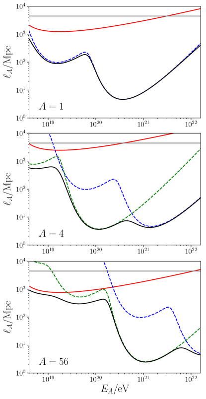
Figure 1: The characteristic lengths of energy-loss for nuclei traversing through background (CMB and EBL) cosmological radiation fields at $z=0$, for various cooling and absorption processes. Panels from top to bottom correspond to protons (¹H) , Helium (⁴He) and Iron (⁵⁶Fe) CR nuclei. Adiabatic losses due to cosmological expansion are represented by the grey lines; pair production by the red curves; photo-pion production by the blue dashed curves; and photo-spallation by the green dashed curves. Here, solid lines and curves denote continuous cooling loss, and dashed curves denote absorptive cooling loss. The solid black curves represent the total cooling.

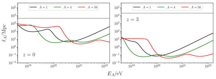
Figure 2: Total characteristic energy-loss distances of CR protons (¹H, black curves), Helium (⁴He, green curves) and Iron (⁵⁶Fe, red curves) in background (CMB and EBL) cosmological radiation fields at $z=0$ (left panel) and $z=3$ (right panel). The corresponding energy-loss distances for adiabatic cooling due to cosmological expansion (grey lines) are shown for comparison. The cooling losses are stronger at $z=3$, because of a strong CMB radiation field, but the adiabatic losses are less severe.

3 Source populations

We adopt a parametrised model to describe the injection rate of CRs:

$${\mathcal{Q}^{\rm a}}_{\!A}(z,\epsilon_{A},A) ={Q^{\rm a}}_{\!A}(1+z)^{-3}$$

$$=\mathcal{C}_{0}(1+z)^{-3}\psi_{\rm x}(z)\;\!\frac{\mathrm{d}}{\mathrm{d}\epsilon_{A}}\left(\frac{\mathrm{d}{n}^{\star}}{\mathrm{d}t}\right)\ ,$$ (33)

where ${\mathcal{Q}^{\rm a}}_{\!A}$ and ${Q^{\rm a}}_{\!A}$ are the comoving and physical source terms, respectively. The normalisation $\mathcal{C}_{0}$ is discussed in Section 3.2. $\psi_{\rm x}(z)$ is the evolutionary function describing the distribution of a CR source population (the specific model is denoted by ${\rm x}$) with respect to redshift $z$ and is discussed in Section 3.1, and $\mathrm{d}n^{\star}/\mathrm{d}t$ is the volumetric injection rate of CRs by a source in that population.

3.1 Redshift distribution

Four source populations are considered, and defined to a maximum redshift $z_{\rm max}=3$. This maximum redshift is chosen because it would be extremely unlikely that UHE CRs could reach us from greater distances, given their suppression by photo-hadronic interactions with the CMB and radiation emitted from astrophysical objects during their propagation in intergalactic space. Each of the source population models we consider follows a different redshift evolution. The first model (referred to as the star formation rate, or SFR, model) is based on the redshift evolution of cosmic star formation (also adopted by Muzio et al. 2019), and takes the form:

$$\psi_{\rm SFR}(z)=\psi_{\rm SFR}^{0}\;\!\frac{(1+z)^{k_{1}}}{1+[(1+z)/k_{2}]^{k_{3}}}\ ,$$ (34)

where $k_{1}=2.7$, $k_{2}=2.9$ and $k_{3}=5.6$ are empirical fit-parameters inherited from the best-fit function of Madau & Dickinson (2014) (see also Robertson et al., 2015).

Our second model choice is a parameterised redshift distribution of gamma-ray bursts (and is referred to as the GRB model hereafter). It follows the form presented in Wang et al. (2011):

$$\psi_{\rm GRB}(z)=\psi_{\rm GRB}^{0}\;\!(1+z)^{k_{4}}\;\!\psi_{\rm SFR}(z)\ ,$$ (35)

where $k_{4}=1.4$. This is based on indications from Swift observations that the GRB rate is enhanced relative to the SFR at high-redshift (Le & Dermer 2007; see also Yüksel & Kistler 2007).

We introduce a third model to describe an AGN source population (referred to as the AGN source model hereafter). For this, we adopt the parametrisation of Hasinger et al. (2005) (see also Ahlers et al., 2009; Wang et al., 2011; Alves Batista et al., 2019a),

$$\psi_{\rm AGN}(z)=\psi_{\rm AGN}^{0}\left\{\begin{array}[]{ll}(1+z)^{k_{5}}&(z<z_{1})\\ {z_{2}}^{k_{5}}&(z_{1}\leq z<z_{2})\\ {z_{2}}^{k_{5}}\cdot{z_{2}}^{z_{2}-z}&(z\geq z_{2})\end{array}\right.\ ,$$ (36)

where $k_{5}=5.0$, $z_{1}=1.7$, $z_{2}=2.7$, which is largely consistent with the results in the later survey studies on AGN populations, e.g. Silverman et al. (2008); Ajello et al. (2012) (which were both adopted by Jacobsen et al., 2015, in the study of spectral and evolutionary properties of UHE neutrinos), and Ueda et al. (2014). There are various uncertainties in modelling other AGN contributions to the UHE CR flux. While it is unlikely that the results obtained from our parametrised model would need substantial revision, these uncertainties, e.g., those concerning the AGN evolution, could have detectable effects on the spectral properties of UHE CRs at Earth.

As the origins of UHE CRs are still to be determined, some studies adopted a simple power-law parametrisation of the redshift evolution of the source model, in the form $(1+z)^{k_{\rm PLW}}$, where $k_{\rm PLW}$ is a fit parameter to be determined (e.g. Taylor et al., 2015; Aab et al., 2017; Jiang et al., 2020). Although our other three source models are more physically-motivated, for comparison we also consider such a power-law parametrisation (referred to as the PLW model), defined as

$$\psi_{\rm PLW}(z)=\psi_{\rm PLW}^{0}\;\!(1+z)^{k_{\rm PLW}}\ ,$$ (37)

with $k_{\rm PLW}=-1.6$, the best-fit value obtained by Alves Batista et al. (2019a). In Equations (34) - (37), $\psi_{\rm SFR}^{0}$, $\psi_{\rm GRB}^{0}$, $\psi_{\rm AGN}^{0}$ and $\psi_{\rm PLW}^{0}$ are the normalisation constants computed by integrating the respective source distribution over redshift up to a cutoff ($z_{\rm max}=3$). Their resulting values are presented in Table 1, and the redshift evolutionary histories for our four source models are shown in Figure 3.

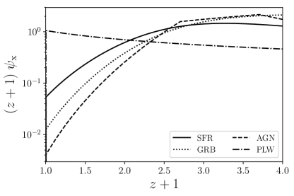
Figure 3: Redshift distributions of the four source models, SFR, GRB, AGN and PLW. Their corresponding normalized redshift evolution functions are given in Equations (34), (35), (36), and (37) respectively.

Table 1: Summary of parameter choices adopted for each of the four redshift source distribution models.

Model	Normalization $\psi_{\rm x}^{0}$	Spectral index $\alpha$	${\rm log}(R_{\rm max}/V)$	$\rho_{\rm CR}$/$10^{48}$ erg Mpc-3 yr-1
(1) SFR	$\psi_{\rm SFR}^{0}=0.054$	$-1.3$	18.2	0.5
(2) GRB	$\psi_{\rm GRB}^{0}=0.013$	$-1.5$	18.2	2.0
(3) AGN	$\psi_{\rm AGN}^{0}=0.0041$	$-1.0$	18.2	0.04
(4) PLW	$\psi_{\rm PLW}^{0}=1.1$	$+1.0$	18.7	15.0

Note. — See text for the choices of the model parameters.

Figure 4: Injection spectra at $z=0$ for the four UHE CR source models, SFR, GRB, AGN and PLW as described in Section 3. ${\mathcal{Q}^{\rm a}}_{\!A}$ is the comoving source term that specifies the injection of CRs from the astrophysical sources, as sepcified in Equation (3). The injection composed of four species, with A=1 (¹H), 4 (⁴He), 14 (¹⁴N) and 28 (²⁸Si), are shown. Their abundances are listed in Table 2 (which are the best fit values from Alves Batista et al. 2019a).

3.2 Cosmic ray luminosity density

The normalisation term $\mathcal{C}_{0}$ in Equation (3) can be determined from the UHE CR luminosity density, $\rho_{\rm CR}$. This is the rate of UHE CR energy density generated by the source population and, at $z=0$, it may be expressed as

$$\rho_{\rm CR} =\mathcal{C}_{0}\sum_{A}\int_{\epsilon_{\mathrm{min}}}^{\epsilon_{\mathrm{max}}}\mathrm{d}\;\!\epsilon_{A}\;\!\epsilon_{A}\;\!\psi_{\rm x}(z)\;\!\frac{\mathrm{d}}{\mathrm{d}\;\!\epsilon_{A}}\left(\frac{\mathrm{d}\;\!{n}^{\star}}{\mathrm{d}\;\!t}\right)\biggr{|}_{z=0}$$ (38)

(cf. Jiang et al., 2020). The exact value of $\rho_{\rm CR}$ is poorly constrained, however it may be roughly estimated by dividing the measured UHE CR energy density at $z=0$, around $10^{54}~{}{\rm erg}~{}{\rm Mpc}^{-3}~{}{\rm dex}^{-1}$ (see Aab et al., 2020), by a typical CR energy loss time, $\ell/c\sim 1~{}{\rm Gpc}/c\sim 1~{}{\rm Gyr}$ (cf. Figure 1), giving $\sim 10^{45}\;\!\text{erg}\;\!\text{Mpc}^{-3}\;\!\text{yr}^{-1}$. This is comparable with more rigorous calculations (e.g. Berezinsky et al., 2006; Aloisio et al., 2007; Wang et al., 2011; Jiang et al., 2020), although the exact number is dependent on assumed model parameters – in particular, the lower energy cut-off of the CR spectrum, and the redshift distribution of the sources (Wang et al., 2011; Jiang et al., 2020). This variation is evident, as shown in the studies of Berezinsky et al. (2006) and Aloisio et al. (2007), where substantially larger values than our estimate, of $3.5\times 10^{46}~{}\text{erg}\;\!\text{Mpc}^{-3}\;\!\text{yr}^{-1}$ and $7\times 10^{46}~{}\text{erg}\;\!\text{Mpc}^{-3}\;\!\text{yr}^{-1}$ (at energies above $10^{18}~{}{\rm eV}$) respectively, are derived by assuming that there is no redshift dependence in the UHE CR source populations. By contrast, much lower values, in the range $0.2-2\times 10^{44}~{}\text{erg}\;\!\text{Mpc}^{-3}\;\!\text{yr}^{-1}$ (at $3.16\times 10^{19}~{}{\rm eV}$) were obtained by Jiang et al. (2020), who adopted a negative redshift evolution for the UHE CR sources population. In Wang et al. (2011), a range of values depending on the assumed source model and energy cut-off are presented: for energies above $10^{18}~{}{\rm eV}$, they found the source luminosity density to be $\sim 0.3-1\times 10^{45}~{}\text{erg}\;\!\text{Mpc}^{-3}\;\!\text{yr}^{-1}$, for a source redshift distribution following that in Yüksel et al. 2008 (corresponding to the SFR scenario in this work); $\sim 6\times 10^{44}~{}\text{erg}\;\!\text{Mpc}^{-3}\;\!\text{yr}^{-1}$ assuming a redshift distribution following the AGN scenario as in this work – cf Equation (36); and $\sim 0.8-3\times 10^{45}\;\!\text{erg}\;\!\text{Mpc}^{-3}\;\!\text{yr}^{-1}$ assuming a source distribution following that of Yüksel & Kistler (2007) (cf. the GRB source scenario considered here). While we do not perform detailed model fitting, we set the UHE CR luminosity density for each of the source models to give a reasonable flux at $z=0$ when compared to Pierre Auger Observatory data (Verzi, 2019) – see Figure 5 and Figure 6. The adopted values (at energies above $5\times 10^{18}\;\!\text{eV}$) are shown in Table 1 for each of the source models, and these were used to set the normalisation $\mathcal{C}_{0}$ in Equation (38) above.

3.3 Source spectrum

We model the energy spectrum of the injected CRs using the spectral form:

$$\frac{\mathrm{d}\;\!n^{\star}}{\mathrm{d}\;\!\epsilon_{A}} \propto f_{A}\left(\frac{\epsilon_{A}}{\epsilon_{\rm min}}\right)^{-\alpha}\left\{\begin{array}[]{ll}1&(x<1)\\ \exp\left(1-x\right)&(x\geq 1)\end{array}\right.\$$ (41)

(Taylor et al., 2015; Alves Batista et al., 2019a; Jiang et al., 2020), where $x={\epsilon_{\rm A}m_{\rm e}c^{2}}/{Z_{A}R_{\max}}$, $R_{\rm max}(V)$ is the rigidity and the energy limits $\epsilon_{\mathrm{min}}m_{\rm e}c^{2}$ and $\epsilon_{\mathrm{max}}m_{\rm e}c^{2}$ retain their earlier values. Our parameter choices for the spectral index $\alpha$ and rigidity are shown in Table 1. Our adopted values are comparable to those derived from fits to Pierre Auger Observatory data in the analysis of Alves Batista et al. (2019a). We note that $\alpha$ is strongly dependent on the adopted source population’s redshift evolution (see Taylor et al., 2015), leading to substantial differences in our choice of parameter value between the four models.

Table 2: Abundance fractions adopted in the model for the four different UHE CR source redshift distributions.

$\psi_{\rm x}(z)$ model	$f_{\rm 1}$ (1H)	$f_{\rm 4}$ (4He)	$f_{\rm 14}$ (14N)	$f_{\rm 28}$ (28Si)	$f_{\rm 56}$ (56Fe)
(1) SFR	0.1628	0.8046	0.0309	0.0018	0.0
(2) GRB	0.5876	0.3973	0.0147	0.0004	0.0
(3) AGN	0.8716	0.0778	0.0469	0.0038	0.0
(4) PLW	0.0003	0.0101	0.8906	0.0990	0.0

3.4 Injected composition

We adopt a simplified CR composition source model, where the full range of injected species are represented by the abundances of ¹H, ⁴He, ¹⁴N, ²⁸Si and ⁵⁶Fe. The individual component spectral forms are indicated in Figure 4, and their total contribution is normalised such that $f_{1}+f_{4}+f_{14}+f_{28}+f_{56}=1$. The fitted composition fraction values obtained by Alves Batista et al. (2019a) are adopted for species abundances for each of the four source populations (SFR, GRB, AGN and PLW). The CR spectral models used in Alves Batista et al. (2019a) and this work are slightly different, but the fitted values given in Alves Batista et al. (2019a) are still a reasonable choice for our model. Note that we calculate the production of all secondary nuclear CR species between ¹H and ⁵⁶Fe formed as the primary UHE CRs propagate and interact with cosmological radiation fields. The abundance fractions of the species used in our calculations are shown in Table 2.

4 Results and Discussion

4.1 Cosmic ray spectrum & composition

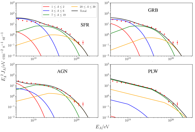
Figure 5: Flux spectra of CRs for the four source models, SFR, GRB, AGN and PLW, propagated to $z=0$. The flux spectrum shown for the assigned range of $A$ has accounted for the production of secondary particles along the CR propagation. The data (discrete red data points with error bars) obtained by the Pierre Auger Observatory (Verzi, 2019) are shown for comparison. The heaviest species of nucleus injected by the sources considered here is ²⁸Si in all the four models, i.e. all the nuclei have mass number ${\rm A}\leqslant 28$. The contribution from particles with $40\leqslant A\leqslant 56$ is therefore zero.

The CR spectrum, expected to be observed at $z=0$, was computed by solving the transport equation (Equation (13) in Section 2.2) numerically using a Runge-Kutta integrator. Cases for the four source populations, SFR, GRB, AGN and PLW, were calculated, with the numerical integration proceeding from $z_{\rm max}=3$ to $z_{\rm min}=0$, with an explicit treatment of the injection of the CR compositions and of the evolution of the source populations along $z$. The computed CR flux and composition at $z=0$ took account of CR propagation and interaction effects, including cooling, absorption and disintegration/spallation (outlined in Section 2). The results are are presented in Figure 5.

The production of secondary nuclei by photo-spallation when CRs propagate in intergalactic space drives the evolution of the composition of CRs, with heavy nuclei gradually being eroded to spawn lighter nuclear species, i.e those of smaller atomic numbers. When the CRs are injected in our model, they are comprised of five nuclear species (i.e. ¹H, ⁴He, ¹⁴N, ²⁸Si and ⁵⁶Fe) as specified by the source models (see Section 3.4). Other species are produced via spallation as the CRs propagate from their sources to $z=0$. This evolution is captured in Figure 5, which shows the compositions in four broad bands to represent the binned distribution of nuclear species when the CRs complete their journey to reach $z=0$.

When setting the abundance of ⁵⁶Fe to be zero, the heaviest species injected by the source model (see Section 3) is ²⁸Si ($A=28$), so no CR nuclei would have $A>28$. As the CRs propagate, nuclei initially having $A=28$ would become nuclei with $A\leq 28$. The four broad-band composition spectra in Figure 5 and the corresponding four injection species spectra in Figure 4 have strikingly similar morphology and relative strengths. The flux in the band $1\leq A\leq 2$ is marginally higher, relatively, than the injected H fraction by the source model, while that in the and $3\leq A\leq 6$, $7\leq A\leq 19$ and $20\leq A\leq 39$ is marginally lower than the injected fractions of ⁴He, ¹⁴N and ²⁸Si respectively. At $z=0$ the flux in each band is dominated by the injected source species, indicating that the evolution of species in an ensemble of CR nuclei propagating over vast distances through intergalactic space is only marginal (subject to the effects of cosmological expansion, cooling, absorption, and photo-spallation). We may therefore conclude that, in the absence of other additional factors, CR species arriving at $z=0$ are overwhelmingly primary CRs rather than secondaries re-processed by photo-spallation. This result is not particularly surprising given that the injection process persists to $z=0$, and the rate of photo-spallation interactions is not comparable to the injection of primary CRs by the sources for the four populations considered. It also explains the limited evolution seen between the injected source spectrum and the post-propagation spectrum, with cooling rates being easily overcome by new injections at all energies (see Figure 1, which also clarifies that absorption processes dominate over any cooling process for CRs with energy above $10^{20}~{}{\rm eV}$).

Our calculations for all considered models yield similar spectra at $z=0$ to that obtained by observations, and this agreement is evident (see Figure 5) when comparing the computed total flux spectra with data obtained by the Pierre Auger Observatory (PAO) (Verzi, 2019). Figure 6 shows a comparison between the total flux spectra obtained for the four models, SFR, GRB, AGN and PLW. The AGN source population model was found to produce (summed) spectra best matching the observation, while the flux levels in all four model cases are similar to the PAO observations and other studies (e.g. Alves Batista et al., 2019a). We note that an improved fit cannot be achieved with the parameter range considered in our models. Model refinement to obtain a better fit with available data is left to future studies.

Figure 7 further compares the average UHE CR spectral mass composition, $\langle{\rm ln}A\rangle$, for the four source classes with data (Pierre Auger Collaboration, 2013; Yushkov, 2019). This shows a clearer distinction between the different source classes, and also clearly rules out the PLW model as parametrised with Equation (37). The AGN model is also disfavored in this comparison (particularly at around $E_{\rm A}\sim 10^{19}\;\!{\rm eV}$), however possible variations in the adopted hadronic model, or the possibility of combined source classes with a refined AGN-type component may offer scope for an improved fit.

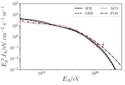
Figure 6: Flux spectra of CRs for the source models, SFR, GRB, AGN and PLW. In each model, the flux is the total value obtained by summing the contributions of all the species considered in the calculations. The data (discrete red data points with error bars) obtained by the Pierre Auger Observatory (Verzi, 2019) are shown for comparison.

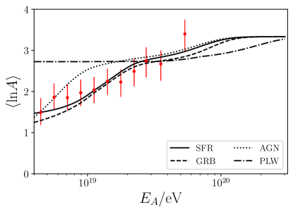
Figure 7: Average UHE CR mass composition, $\langle{\rm ln}A\rangle$, for the four source classes, compared to data obtained with the Pierra Auger Observatory (Pierre Auger Collaboration, 2013; Yushkov, 2019) when adopting the Sibyll 2.3c hadronic interaction model (Riehn et al., 2017).

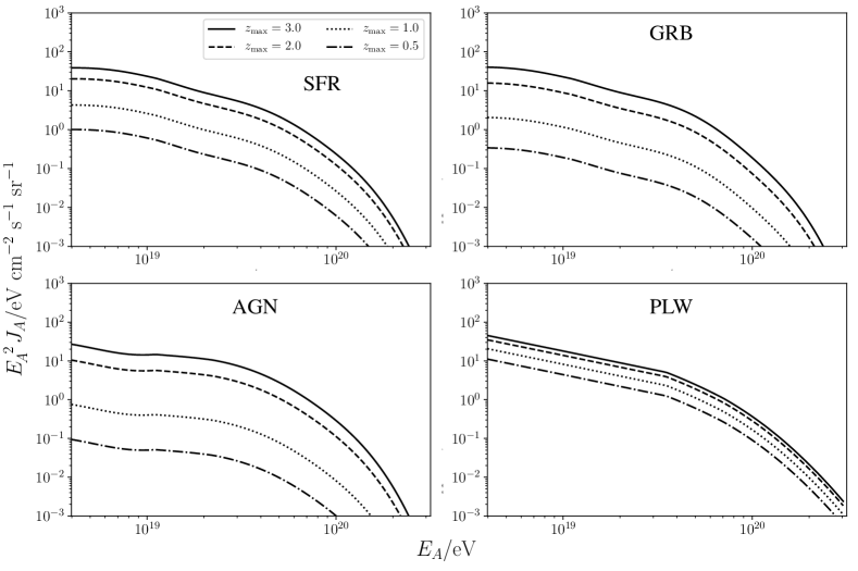
Figure 8: Total flux spectra of CRs propagated to $z=0$ for the four source models. In each model, the cases for CR injection truncated at redshifts $z_{\rm max}=0.5$, 1.0, 2.0 and 3.0 (curves from bottom to top) are shown. Comparing the flux spectra for different redshift truncation reveals that the contributions from distance sources are significant.

4.2 Contributions from distant UHE CR sources

Anisotropy in the arrival directions of UHE CRs above $8\times 10^{18}~{}{\rm eV}$, at a significance $>5.2\sigma$ was recently reported (see Abreu et al., 2010; Aab et al., 2014, 2015; Pierre Auger Collaboration et al., 2017; Aab et al., 2018; Abbasi et al., 2018). There are also indications of correlations with certain candidate high-energy cosmic accelerators (see Pierre Auger Collaboration et al., 2007; Abreu et al., 2010), which include AGN detected in $\gamma$-rays and X-rays (Nemmen et al., 2010; Terrano et al., 2012), as well as source distributions tracing large-scale structures, with a source population being biased with respect to the distribution of galaxies (Kashti & Waxman, 2008). A CR ‘hotspot’ was recently reported by Abbasi et al. (2014). Studies by Fang et al. (2014) and He et al. (2016) showed that this hotspot is consistent with a single source rather than a chance signal. Clusters of excess arrivals of UHE CRs above an isotropic background from the direction of Centaurus A have been found in some analyses (Fargion & D’Armiento, 2011; Kim, 2013a, b). However, there is no clear detection of excesses around other nearby radio galaxies, e.g. Centaurus B and Virgo A (see Fraija et al., 2019; Kobzar et al., 2019).

If UHE CRs are produced by sources located nearby to our Galaxy with a fraction originating from within the conventional GZK horizon, as well as sources at large (cosmological) distances, then their arrival flux could have two components: an isotropic component corresponding to unresolved distant sources and an anisotropic component associated with relatively nearby sources. The reported anisotropies detected in UHE CRs are consistent with this scenario, and consideration of a foreground and background component in the UHE CR flux was shown in Kim & Kim (2011) to improve anisotropy correlations with the positions of potential nearby sources. This is complimented by the blind test performed by Rubtsov et al. (2012) for verifying the hypothesis that AGN were the origin of UHE CRs, using event sets from Yakutsk, AGASA and HiRes. Their findings were consistent with a random background (see also High Resolution Fly’S Eye Collaboration et al., 2008, which also found 13 UHE CR events detected by HiRes in the northern hemisphere to be consistent with isotropy).

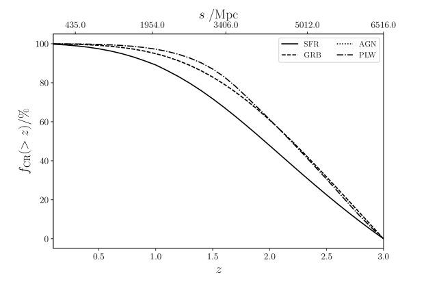
Figure 9: The fraction of CRs that originate from redshift higher than $z$, $f_{\rm CR}(>z)$, for the four source models. The bottom abscissa shows the redshift $z$, and the top abscissa the corresponding comoving distances, for the cosmological model with $\Omega_{\rm m,0}=0.315\pm 0.007$, $\Omega_{\rm r,0}\approx 0$, $\Omega_{\rm\Lambda,0}=0.685\pm 0.007$, and $h=0.673\pm 0.006$ (see Section 2.2). The curves for the GRB and AGN models are almost indistinguishable, a consequence of the redshift evolution of GRB and AGN, in that most contributions from their respective sources are located at similar redshifts (see Figure 3).

Here, we assess the fraction of UHE CR flux that could originate at large distances, from sources located beyond a GZK ‘horizon’ distance of a few tens Mpc (see e.g. Kachelrieß & Semikoz, 2019), and determine their contribution to a UHE CR background. Distant CR sources are homogeneously distributed across the celestial sphere over a range redshifts. Regardless the fraction of their flux which can survive to reach Earth, CRs originating from these sources should not, at least in principle, show resolvable anisotropy. To assess the relative contributions to the CRs observed at $z=0$ from the CRs initially produced by distant sources at different redshifts, we computed the flux spectra (for each of the source models) with several assigned $z_{\rm max}$, taking values from 3.0, 2.0, 1.0 and 0.5. The spectra computed at $z=0$ for four source models are presented in Figure 8 for four values of $z_{\rm max}$. This shows that changing either the source model or $z_{\rm max}$ leads to discernible changes in the spectra at $z=0$. The contribution of distant source populations is clearly substantial and naturally accounts for the emergence of an isotropic (background) component in the observed UHE CR flux on Earth.

The significance of the distant sources’ contribution varies among the different source evolution models, which can be seen from comparing the set of spectra of different $z_{\rm max}$ shown in different panels of Figure 8. The amount of reduction between the spectrum from sources below $z=3$ to that from sources below $z=2$ accounts for a large fraction of the total CR flux arriving at $z=0$, which is at a level between 30$-$50% in the SFR, GRB and AGB models. The PLW model however, has a relatively smaller reduction in the flux for the same redshift interval, implying that CR flux is dominated by sources at lower redshifts in that case.

Figure 9 shows the fractional contribution from sources above a given redshift, $f_{\rm CR}(>z)$, for the four source models. Most noticeably, the curves for the GRB and AGN models are practically indistinguishable. The morphology of the $f_{\rm CR}(>z)$ curve is a manifestation of the redshift locations where a specific population of sources has the most significant contribution. The dominant redshift locations of the GRB and AGN CR sources are very similar to one another (cf. the curves of these two source populations in Figure 3, particularly above $(z+1)\approx 2.5$). This, together with the lacking of substantial numbers of GRB and AGN below $(z+1)\sim 2.5$ leads to their almost identical $f_{\rm CR}(>z)$ curves. Figure 9 indicates that, for all the source population models considered, a large faction of UHE CR flux observed at Earth would originate from regions far beyond the conventional GZK horizon of a few tens Mpc, and would not be attributed to local sources. If the UHE CRs are predominantly produced as a consequence of star formation, which is represented by the SFR model here, then $\sim\;\!50$% of the CRs could originate from as far as $z\sim 2$ or above.

These findings are robust. The results obtained from our calculations are not sensitive to the assumed composition of the injected UHE CR flux. The outcome is similar even if the CR injections are restricted to a single species (of any of the five nuclei considered). This is in line with the chemical evolution due to photo-spallation processes being insignificant, otherwise, the composition evolution of CRs would be strongly manifested in the CR energy spectra of the species observed at Earth.

5 Summary and Conclusions

In this work we investigated the UHE CR flux and spectra at $z=0$ with the explicit considerations of (i) the distribution of candidate sources in the cosmological context (modeled as four different redshift-dependent populations, denoted as SFR, GRB, AGN and PLW as described in previous sections), (ii) the composition of the injected CR nuclear species (specified by the abundance of ¹H, ⁴He, ²⁸Si and ⁵⁶Fe species), and (iii) the relevant radiative and cooling processes, and particle absorption interactions (which include photo-spallation for the CR nuclei when interacting with CMB and EBL radiation fields). We solved the particle transport equations numerically and determined the evolution of CR properties, in particular the CR flux and spectra and the compositions of species for each model. Our calculations have shown that sources at redshifts as high as $z\sim(2-3)$ can contribute substantially to UHE CRs detected on Earth, with different source classes being distinguishable using the average UHE CR mass composition spectrum at $z=0$. Comparison with average CR mass data obtained from the Pierre Auger Observatory allowed a strong contribution from a PLW-type source population (as parametrised with Equation 37) to be ruled out.

Regardless of population class, we find that most of the UHE CRs from these distant source populations are primary particles, despite the large cosmological distances that they have traversed. These UHE CRs are diffuse and isotropic, as they are of cosmological origin. They constitute the isotropic background on which an anisotropic UHE CR component associated with the nearby CR accelerators is superimposed.

Appendix A Extra-galactic background light

Table 3: Summary of parameter choices for $z=0$ EBL model, approximating an upper-estimate for the EBL using blackbody components (Hauser & Dwek, 2001). Dimensionless weights $f_{i,0}$ have been estimated from relative normalisations.

Componenta	T/K	$\Theta_{i}$	$f_{i,0}$
Dust	62	$1.1\times 10^{-8}$	$3.5\times 10^{-7}$
UV/O (1)	400	$6.7\times 10^{-8}$	$9.0\times 10^{-12}$
UV/O (2)	1,000	$1.7\times 10^{-7}$	$4.5\times 10^{-13}$
UV/O (3)	3,000	$5.1\times 10^{-7}$	$1.4\times 10^{-14}$
UV/O (4)	5,500	$9.3\times 10^{-7}$	$6.0\times 10^{-16}$
UV/O (5)	12,000	$2.0\times 10^{-6}$	$6.1\times 10^{-17}$

Extra-galactic background light is comprised of radiation emitted from astrophysical objects. Its energy is mainly concentrated in two spectral peaks – one at optical wavelengths, being broadly associated with stellar emission from within populations of galaxies, while the other is at infra-red wavelengths, and is presumably dominated by dust-reprocessed astrophysical emission (also mainly originating from within galaxies).

The EBL is well-studied observationally in the local Universe (see Cooray, 2016). However, its redshift evolution is less well-constrained (for EBL constraints from observations over a range of redshifts, see e.g. Franceschini & Rodighiero, 2017), and is determined by the evolution of its astrophysical source populations. While many approaches have been taken to model the cosmological evolution of the EBL in detail, including forward-evolutionary models (e.g. Kneiske & Dole, 2010; Finke et al., 2010), backward-evolutionary models (e.g. Domínguez et al., 2011; Stecker et al., 2012), and semi-analytical models (e.g. Gilmore et al., 2012; Inoue et al., 2013), these are each subject to certain inherent assumptions and uncertainties leading to substantial variations in predictions between models and modeling approaches. Although the EBL has been shown to affect the cosmological propagation of UHE CRs (e.g. Allard et al., 2005; Aloisio et al., 2013b), and the exact form of model adopted has been demonstrated to have non-negligible effects on the spectrum of UHE CRs (e.g. Aloisio et al., 2013b), we do not find it to have substantial impacts on the results of this study, with any EBL model (if reasonable) yielding comparable results. We therefore adopt a simple analytic representation of the EBL, comprised of six superposed blackbody components, as listed in Table 3. Of these, one is attributed to dust (infrared) emission and the remaining five are a non-physical approximation to the UV/optical part of the EBL that presumably arises from stellar emission. Of these five, only the components ‘UV/O (1)’ and ‘UV/O (2)’ fall within the photon energy range relevant to our calculations. The components $i$ each take the form

$$n_{i}(\epsilon_{\rm ph},z)=\frac{8\pi\;\!f_{i}(z)}{\lambda_{\rm c}^{3}}\frac{\epsilon_{\rm ph}^{2}}{\exp(\epsilon_{\rm ph}/{\Theta}_{i})-1}\ ,$$ (A1)

where terms retain their earlier definitions. The redshift-dependent dimensionless weights of the components are

$$f_{i}(z)=f_{i,0}\;\begin{cases}(1+z)^{3.1}\ ,\hskip 25.6073ptz<z_{\rm cut}\\ (1+z_{\rm cut})^{3.1}\ ,\hskip 14.22636ptz\geq z_{\rm cut}\end{cases}\ ,$$ (A2)

up to $z=3$, where $z_{\rm cut}=1.4$, which follows the ‘baseline’ EBL redshift evolution model in Aloisio et al. (2013b). More detailed investigation of the impact of the redshift evolution of the EBL on UHE CR propagation falls beyond the scope of this paper, and is more appropriate for a dedicated future study. Temperature, energy density, dimensionless temperature $\Theta_{i}$ and $z=0$ dimensionless weights $f_{i,0}$ for each EBL model component $i$ are listed in Table 3. These choices have been shown to give reasonable consistency with local observational constraints (Hauser & Dwek, 2001). Note that, for comparison, in the case of the CMB, $f=1$ and $\Theta(z)=4.58\times 10^{-10}\;\!(1+z)$.

References

- Aab et al. (2014) Aab, A., Abreu, P., Aglietta, M., et al. 2014, ApJ, 794, 172, doi: 10.1088/0004-637X/794/2/172
- Aab et al. (2015) —. 2015, ApJ, 804, 15, doi: 10.1088/0004-637X/804/1/15
- Aab et al. (2017) —. 2017, J. Cosmology Astropart. Phys, 2017, 038, doi: 10.1088/1475-7516/2017/04/038
- Aab et al. (2018) —. 2018, ApJ, 868, 4, doi: 10.3847/1538-4357/aae689
- Aab et al. (2020) —. 2020, Phys. Rev. Lett., 125, 121106, doi: 10.1103/PhysRevLett.125.121106
- Abbasi et al. (2014) Abbasi, R. U., Abe, M., Abu-Zayyad, T., et al. 2014, ApJ, 790, L21, doi: 10.1088/2041-8205/790/2/L21
- Abbasi et al. (2018) —. 2018, ApJ, 858, 76, doi: 10.3847/1538-4357/aabad7
- Abreu et al. (2010) Abreu, P., Aglietta, M., Ahn, E. J., et al. 2010, Astroparticle Physics, 34, 314, doi: 10.1016/j.astropartphys.2010.08.010
- Abu-Zayyad et al. (2013) Abu-Zayyad, T., Aida, R., Allen, M., et al. 2013, ApJ, 768, L1, doi: 10.1088/2041-8205/768/1/L1
- Ahlers et al. (2009) Ahlers, M., Anchordoqui, L. A., & Sarkar, S. 2009, Phys. Rev. D, 79, 083009, doi: 10.1103/PhysRevD.79.083009
- Ahlers & Salvado (2011) Ahlers, M., & Salvado, J. 2011, Phys. Rev. D, 84, 085019, doi: 10.1103/PhysRevD.84.085019
- Ajello et al. (2012) Ajello, M., Shaw, M. S., Romani, R. W., et al. 2012, ApJ, 751, 108, doi: 10.1088/0004-637X/751/2/108
- Allard et al. (2006) Allard, D., Ave, M., Busca, N., et al. 2006, J. Cosmology Astropart. Phys, 2006, 005, doi: 10.1088/1475-7516/2006/09/005
- Allard et al. (2005) Allard, D., Parizot, E., Olinto, A. V., Khan, E., & Goriely, S. 2005, A&A, 443, L29, doi: 10.1051/0004-6361:200500199
- Aloisio et al. (2014) Aloisio, R., Berezinsky, V., & Blasi, P. 2014, J. Cosmology Astropart. Phys, 2014, 020, doi: 10.1088/1475-7516/2014/10/020
- Aloisio et al. (2007) Aloisio, R., Berezinsky, V., Blasi, P., et al. 2007, Astroparticle Physics, 27, 76, doi: 10.1016/j.astropartphys.2006.09.004
- Aloisio et al. (2013a) Aloisio, R., Berezinsky, V., & Grigorieva, S. 2013a, Astroparticle Physics, 41, 73, doi: 10.1016/j.astropartphys.2012.07.010
- Aloisio et al. (2013b) —. 2013b, Astroparticle Physics, 41, 94, doi: 10.1016/j.astropartphys.2012.06.003
- Álvarez et al. (2016) Álvarez, E., Cuoco, A., Mirabal, N., & Zaharijas, G. 2016, J. Cosmology Astropart. Phys, 2016, 023, doi: 10.1088/1475-7516/2016/12/023
- Alves Batista et al. (2019a) Alves Batista, R., de Almeida, R. M., Lago, B., & Kotera, K. 2019a, J. Cosmology Astropart. Phys, 2019, 002, doi: 10.1088/1475-7516/2019/01/002
- Alves Batista et al. (2013) Alves Batista, R., Erdmann, M., Evoli, C., et al. 2013, in International Cosmic Ray Conference, Vol. 33, International Cosmic Ray Conference, 694. https://arxiv.org/abs/1307.2643
- Alves Batista et al. (2019b) Alves Batista, R., Biteau, J., Bustamante, M., et al. 2019b, Frontiers in Astronomy and Space Sciences, 6, 23, doi: 10.3389/fspas.2019.00023
- Berezinsky et al. (2006) Berezinsky, V., Gazizov, A., & Grigorieva, S. 2006, Phys. Rev. D, 74, 043005, doi: 10.1103/PhysRevD.74.043005
- Berezinsky & Gazizov (1993) Berezinsky, V. S., & Gazizov, A. Z. 1993, Phys. Rev. D, 47, 4206, doi: 10.1103/PhysRevD.47.4206
- Berezinsky & Grigor’eva (1988) Berezinsky, V. S., & Grigor’eva, S. I. 1988, A&A, 199, 1
- Bethe & Heitler (1934) Bethe, H., & Heitler, W. 1934, Proc. R. Soc. A, 146, 83, doi: 10.1098/rspa.1934.0140
- Bethe & Maximon (1954) Bethe, H. A., & Maximon, L. C. 1954, Physical Review, 93, 768, doi: 10.1103/PhysRev.93.768
- Bird et al. (1994) Bird, D. J., Corbato, S. C., Dai, H. Y., et al. 1994, ApJ, 424, 491, doi: 10.1086/173906
- Bird et al. (1995) —. 1995, ApJ, 441, 144, doi: 10.1086/175344
- Blumenthal (1970) Blumenthal, G. R. 1970, Phys. Rev. D, 1, 1596, doi: 10.1103/PhysRevD.1.1596
- Cooray (2016) Cooray, A. 2016, Royal Society Open Science, 3, 150555, doi: 10.1098/rsos.150555
- Deligny et al. (2017) Deligny, O., Kawata, K., & Tinyakov, P. 2017, Progress of Theoretical and Experimental Physics, 2017, doi: 10.1093/ptep/ptx043
- Dermer & Menon (2009) Dermer, C. D., & Menon, G. 2009, High energy radiation from black holes: gamma rays, cosmic rays, and neutrinos, Princeton series in astrophysics (Princeton, NJ: Princeton University Press)
- Domínguez et al. (2011) Domínguez, A., Primack, J. R., Rosario, D. J., et al. 2011, MNRAS, 410, 2556, doi: 10.1111/j.1365-2966.2010.17631.x
- Fang et al. (2014) Fang, K., Fujii, T., Linden, T., & Olinto, A. V. 2014, ApJ, 794, 126, doi: 10.1088/0004-637X/794/2/126
- Fargion & D’Armiento (2011) Fargion, D., & D’Armiento, D. 2011, in Italian Physical Society Conference Proceedings, Vol. 103, Italian Physical Society Conference Proceedings. https://arxiv.org/abs/1101.0273
- Finke et al. (2010) Finke, J. D., Razzaque, S., & Dermer, C. D. 2010, ApJ, 712, 238, doi: 10.1088/0004-637X/712/1/238
- Fraija et al. (2019) Fraija, N., Araya, M., Galván-Gámez, A., & de Diego, J. A. 2019, J. Cosmology Astropart. Phys, 2019, 023, doi: 10.1088/1475-7516/2019/08/023
- Franceschini & Rodighiero (2017) Franceschini, A., & Rodighiero, G. 2017, A&A, 603, A34, doi: 10.1051/0004-6361/201629684
- Giacinti et al. (2012) Giacinti, G., Kachelrieß, M., Semikoz, D. V., & Sigl, G. 2012, J. Cosmology Astropart. Phys, 2012, 031, doi: 10.1088/1475-7516/2012/07/031
- Gilmore et al. (2012) Gilmore, R. C., Somerville, R. S., Primack, J. R., & Domínguez, A. 2012, MNRAS, 422, 3189, doi: 10.1111/j.1365-2966.2012.20841.x
- Gould (1975) Gould, R. J. 1975, ApJ, 196, 689, doi: 10.1086/153457
- Gould (1993) —. 1993, ApJ, 417, 12, doi: 10.1086/173287
- Greisen (1966) Greisen, K. 1966, Phys. Rev. Lett., 16, 748, doi: 10.1103/PhysRevLett.16.748
- Hasinger et al. (2005) Hasinger, G., Miyaji, T., & Schmidt, M. 2005, A&A, 441, 417, doi: 10.1051/0004-6361:20042134
- Hauser & Dwek (2001) Hauser, M. G., & Dwek, E. 2001, ARA&A, 39, 249, doi: 10.1146/annurev.astro.39.1.249
- Hayward (1960) Hayward, E. 1960, Science, 132, 951, doi: 10.1126/science.132.3432.951-a
- He et al. (2016) He, H.-N., Kusenko, A., Nagataki, S., et al. 2016, Phys. Rev. D, 93, 043011, doi: 10.1103/PhysRevD.93.043011
- High Resolution Fly’S Eye Collaboration et al. (2008) High Resolution Fly’S Eye Collaboration, Abbasi, R. U., Abu-Zayyad, T., et al. 2008, Astroparticle Physics, 30, 175, doi: 10.1016/j.astropartphys.2008.08.004
- Hillas (1984) Hillas, A. M. 1984, ARA&A, 22, 425, doi: 10.1146/annurev.aa.22.090184.002233
- Hümmer et al. (2010) Hümmer, S., Rüger, M., Spanier, F., & Winter, W. 2010, ApJ, 721, 630, doi: 10.1088/0004-637X/721/1/630
- Inoue et al. (2013) Inoue, Y., Inoue, S., Kobayashi, M. A. R., et al. 2013, ApJ, 768, 197, doi: 10.1088/0004-637X/768/2/197
- Ivanov (2017) Ivanov, D. 2017, PoS, ICRC2017, 498, doi: 10.22323/1.301.0498
- Jacobsen et al. (2015) Jacobsen, I. B., Wu, K., On, A. Y. L., & Saxton, C. J. 2015, MNRAS, 451, 3649, doi: 10.1093/mnras/stv1196
- Jiang et al. (2020) Jiang, Y., Zhang, B. T., & Murase, K. 2020, arXiv e-prints, arXiv:2012.03122. https://arxiv.org/abs/2012.03122
- Jost et al. (1950) Jost, R., Luttinger, J. M., & Slotnick, M. 1950, Phys. Rev., 80, 189, doi: 10.1103/PhysRev.80.189
- Kachelrieß & Semikoz (2019) Kachelrieß, M., & Semikoz, D. V. 2019, Progress in Particle and Nuclear Physics, 109, 103710, doi: 10.1016/j.ppnp.2019.07.002
- Kalashev et al. (2008) Kalashev, O. E., Khrenov, B. A., Klimov, P., Sharakin, S., & Troitsky, S. V. 2008, J. Cosmology Astropart. Phys, 2008, 003, doi: 10.1088/1475-7516/2008/03/003
- Kampert et al. (2013) Kampert, K.-H., Kulbartz, J., Maccione, L., et al. 2013, Astroparticle Physics, 42, 41, doi: 10.1016/j.astropartphys.2012.12.001
- Karakula & Tkaczyk (1993) Karakula, S., & Tkaczyk, W. 1993, Astroparticle Physics, 1, 229, doi: 10.1016/0927-6505(93)90023-7
- Kashti & Waxman (2008) Kashti, T., & Waxman, E. 2008, J. Cosmology Astropart. Phys, 2008, 006, doi: 10.1088/1475-7516/2008/05/006
- Kim (2013a) Kim, H. B. 2013a, Journal of Korean Physical Society, 62, 708, doi: 10.3938/jkps.62.708
- Kim (2013b) —. 2013b, ApJ, 764, 121, doi: 10.1088/0004-637X/764/2/121
- Kim & Kim (2011) Kim, H. B., & Kim, J. 2011, J. Cosmology Astropart. Phys, 2011, 006, doi: 10.1088/1475-7516/2011/03/006
- Klein (2006) Klein, S. R. 2006, Radiation Physics and Chemistry, 75, 696, doi: 10.1016/j.radphyschem.2005.09.005
- Kneiske & Dole (2010) Kneiske, T. M., & Dole, H. 2010, A&A, 515, A19, doi: 10.1051/0004-6361/200912000
- Kobzar et al. (2019) Kobzar, O., Hnatyk, B., Marchenko, V., & Sushchov, O. 2019, MNRAS, 484, 1790, doi: 10.1093/mnras/stz094
- Kotera & Olinto (2011) Kotera, K., & Olinto, A. V. 2011, ARA&A, 49, 119, doi: 10.1146/annurev-astro-081710-102620
- Le & Dermer (2007) Le, T., & Dermer, C. D. 2007, ApJ, 661, 394, doi: 10.1086/513460
- Madau & Dickinson (2014) Madau, P., & Dickinson, M. 2014, ARA&A, 52, 415, doi: 10.1146/annurev-astro-081811-125615
- Mirabal & Oya (2010) Mirabal, N., & Oya, I. 2010, MNRAS, 405, L99, doi: 10.1111/j.1745-3933.2010.00868.x
- Moncada et al. (2017) Moncada, R. J., Colon, R. A., Guerra, J. J., O’Dowd, M. J., & Anchordoqui, L. A. 2017, Journal of High Energy Astrophysics, 13, 32, doi: 10.1016/j.jheap.2017.04.001
- Morejon et al. (2019) Morejon, L., Fedynitch, A., Boncioli, D., Biehl, D., & Winter, W. 2019, J. Cosmology Astropart. Phys, 2019, 007, doi: 10.1088/1475-7516/2019/11/007
- Mücke et al. (1999) Mücke, A., Rachen, J. P., Engel, R., Protheroe, R. J., & Stanev, T. 1999, PASA, 16, 160, doi: 10.1071/AS99160
- Muzio et al. (2019) Muzio, M. S., Unger, M., & Farrar, G. R. 2019, Phys. Rev. D, 100, 103008, doi: 10.1103/PhysRevD.100.103008
- Nakamura (2010) Nakamura, K. 2010, Journal of Physics G: Nuclear and Particle Physics, 37, 075021. http://stacks.iop.org/0954-3899/37/i=7A/a=075021
- Nemmen et al. (2010) Nemmen, R. S., Bonatto, C., & Storchi-Bergmann, T. 2010, ApJ, 722, 281, doi: 10.1088/0004-637X/722/1/281
- Ostapchenko (2011) Ostapchenko, S. 2011, Phys. Rev. D, 83, 014018, doi: 10.1103/PhysRevD.83.014018
- Owen et al. (2018) Owen, E. R., Jacobsen, I. B., Wu, K., & Surajbali, P. 2018, MNRAS, 481, 666, doi: 10.1093/mnras/sty2279
- Owen et al. (2021) Owen, E. R., Lee, K.-G., & Kong, A. K. H. 2021, MNRAS, 506, 52, doi: 10.1093/mnras/stab1707
- Owen et al. (2019) Owen, E. R., Wu, K., Jin, X., Surajbali, P., & Kataoka, N. 2019, A&A, 626, A85, doi: 10.1051/0004-6361/201834350
- Palladino et al. (2020) Palladino, A., van Vliet, A., Winter, W., & Franckowiak, A. 2020, MNRAS, 494, 4255, doi: 10.1093/mnras/staa1003
- Peacock (1999) Peacock, J. A. 1999, Cosmological Physics
- Pe’er & Loeb (2012) Pe’er, A., & Loeb, A. 2012, J. Cosmology Astropart. Phys, 2012, 007, doi: 10.1088/1475-7516/2012/03/007
- Pierog et al. (2015) Pierog, T., Karpenko, I., Katzy, J. M., Yatsenko, E., & Werner, K. 2015, Phys. Rev. C, 92, 034906, doi: 10.1103/PhysRevC.92.034906
- Pierre Auger Collaboration (2013) Pierre Auger Collaboration. 2013, J. Cosmology Astropart. Phys, 2013, 026, doi: 10.1088/1475-7516/2013/02/026
- Pierre Auger Collaboration et al. (2007) Pierre Auger Collaboration, Abraham, J., Abreu, P., et al. 2007, Science, 318, 938, doi: 10.1126/science.1151124
- Pierre Auger Collaboration et al. (2017) Pierre Auger Collaboration, Aab, A., Abreu, P., et al. 2017, Science, 357, 1266, doi: 10.1126/science.aan4338
- Planck Collaboration et al. (2020) Planck Collaboration, Aghanim, N., Akrami, Y., et al. 2020, A&A, 641, A6, doi: 10.1051/0004-6361/201833910
- Press et al. (1992) Press, W. H., Teukolsky, S. A., Vetterling, W. T., & Flannery, B. P. 1992, Numerical recipes in FORTRAN. The art of scientific computing
- Protheroe & Johnson (1996) Protheroe, R. J., & Johnson, P. A. 1996, Astroparticle Physics, 4, 253, doi: 10.1016/0927-6505(95)00039-9
- Puget et al. (1976) Puget, J. L., Stecker, F. W., & Bredekamp, J. H. 1976, ApJ, 205, 638, doi: 10.1086/154321
- Rieger (2019) Rieger, F. 2019, in High Energy Phenomena in Relativistic Outflows VII, 19. https://arxiv.org/abs/1911.04171
- Riehn et al. (2017) Riehn, F., Dembinski, H., Fedynitch, A., et al. 2017, PoS, ICRC2017, 301, doi: 10.22323/1.301.0301
- Robertson et al. (2015) Robertson, B. E., Ellis, R. S., Furlanetto, S. R., & Dunlop, J. S. 2015, ApJ, 802, L19, doi: 10.1088/2041-8205/802/2/L19
- Rodrigues et al. (2021) Rodrigues, X., Heinze, J., Palladino, A., van Vliet, A., & Winter, W. 2021, Phys. Rev. Lett., 126, 191101, doi: 10.1103/PhysRevLett.126.191101
- Romero & Gutiérrez (2020) Romero, G., & Gutiérrez, E. 2020, Universe, 6, 99, doi: 10.3390/universe6070099
- Rubtsov et al. (2012) Rubtsov, G. I., Tkachev, I. I., & Dolgov, A. D. 2012, Soviet Journal of Experimental and Theoretical Physics Letters, 95, 501, doi: 10.1134/S0021364012100098
- Silverman et al. (2008) Silverman, J. D., Green, P. J., Barkhouse, W. A., et al. 2008, ApJ, 679, 118, doi: 10.1086/529572
- Stecker (1969) Stecker, F. 1969, Phys. Rev., 180, 1264, doi: 10.1103/PhysRev.180.1264
- Stecker (1979) Stecker, F. W. 1979, ApJ, 228, 919, doi: 10.1086/156919
- Stecker et al. (2012) Stecker, F. W., Malkan, M. A., & Scully, S. T. 2012, ApJ, 761, 128, doi: 10.1088/0004-637X/761/2/128
- Stecker & Salamon (1999) Stecker, F. W., & Salamon, M. H. 1999, ApJ, 512, 521, doi: 10.1086/306816
- Stepney & Guilbert (1983) Stepney, S., & Guilbert, P. W. 1983, MNRAS, 204, 1269, doi: 10.1093/mnras/204.4.1269
- Taylor et al. (2015) Taylor, A. M., Ahlers, M., & Hooper, D. 2015, Phys. Rev. D, 92, 063011, doi: 10.1103/PhysRevD.92.063011
- Terrano et al. (2012) Terrano, W. A., Zaw, I., & Farrar, G. R. 2012, ApJ, 754, 142, doi: 10.1088/0004-637X/754/2/142
- Ueda et al. (2014) Ueda, Y., Akiyama, M., Hasinger, G., Miyaji, T., & Watson, M. G. 2014, ApJ, 786, 104, doi: 10.1088/0004-637X/786/2/104
- Unger et al. (2015) Unger, M., Farrar, G. R., & Anchordoqui, L. A. 2015, Phys. Rev. D, 92, 123001, doi: 10.1103/PhysRevD.92.123001
- Verzi (2019) Verzi, V. 2019, PoS, ICRC2019, 450, doi: 10.22323/1.358.0450
- Wanderman & Piran (2010) Wanderman, D., & Piran, T. 2010, MNRAS, 406, 1944, doi: 10.1111/j.1365-2966.2010.16787.x
- Wang et al. (2011) Wang, X.-Y., Liu, R.-Y., & Aharonian, F. 2011, ApJ, 736, 112, doi: 10.1088/0004-637X/736/2/112
- Wang et al. (2008) Wang, X.-Y., Razzaque, S., & Mészáros, P. 2008, ApJ, 677, 432, doi: 10.1086/529018
- Watson (2014) Watson, A. A. 2014, Reports on Progress in Physics, 77, 036901, doi: 10.1088/0034-4885/77/3/036901
- Webb & Gleeson (1979) Webb, G. M., & Gleeson, L. J. 1979, Ap&SS, 60, 335, doi: 10.1007/BF00644337
- Yüksel & Kistler (2007) Yüksel, H., & Kistler, M. D. 2007, Phys. Rev. D, 75, 083004, doi: 10.1103/PhysRevD.75.083004
- Yüksel et al. (2008) Yüksel, H., Kistler, M. D., Beacom, J. F., & Hopkins, A. M. 2008, ApJ, 683, L5, doi: 10.1086/591449
- Yushkov (2019) Yushkov, A. 2019, PoS, ICRC2019, 482, doi: 10.22323/1.358.0482
- Zatsepin & Kuz’min (1966) Zatsepin, G. T., & Kuz’min, V. A. 1966, Soviet Journal of Experimental and Theoretical Physics Letters, 4, 78