Transfer Learning in Multi-Agent Reinforcement Learning with Double Q-Networks for Distributed Resource Sharing in V2X Communication

Abstract

This paper addresses the problem of decentralized spectrum sharing in vehicle-to-everything (V2X) communication networks. The aim is to provide resource-efficient coexistence of vehicle-to-infrastructure (V2I) and vehicle-to-vehicle (V2V) links. A recent work on the topic proposes a multi-agent reinforcement learning (MARL) approach based on deep Q-learning, which leverages a fingerprint-based deep Q-network (DQN) architecture. This work considers an extension of this framework by combining Double Q-learning (via Double DQN) and transfer learning. The motivation behind is that Double Q-learning can alleviate the problem of overestimation of the action values present in conventional Q-learning, while transfer learning can leverage knowledge acquired by an expert model to accelerate learning in the MARL setting. The proposed algorithm is evaluated in a realistic V2X setting, with synthetic data generated based on a geometry-based propagation model that incorporates location-specific geographical descriptors of the simulated environment (outlines of buildings, foliage, and vehicles). The advantages of the proposed approach are demonstrated via numerical simulations.

I Introduction

In vehicle-to-everything (V2X) networks, vehicle-to-infrastructure (V2I) and vehicle-to-vehicle (V2V) connections are supported through cellular and sidelink radio interfaces respectively. With the introduction of use cases such as tele-operated driving, in-vehicle entertainment and automated driving, V2X networks are required to provide simultaneous support for mobile high-data rates and advanced driving, i.e. safety-related services. For example, while the in-vehicle entertainment applications require high bandwidth V2I connection to the base station (BS), safety applications need to periodically disseminate messages among neighboring vehicles with high reliability and low latency.

To provide resource-efficient coexistence of V2I and V2V connections, sidelink V2V connections may be configured to share spectrum with V2I links. In that case, effective strategies for spectrum sharing with V2I links are required, including the selection of spectrum sub-band and control of transmission power, in order to meet the diverse service requirements of both V2I and V2V links. Furthermore, taking into account the nature of the V2V traffic, decentralized solutions are favored over centralized schemes that come with large transmission overhead and higher latency.

The decentralized spectrum sharing problem can be cast as a multi-agent reinforcement learning (MARL) problem where the V2V links, each acting as an agent, collectively interact with the communication environment and learn to improve spectrum and power allocation by using the gained experiences. Along these lines, a MARL approach based on deep Q-learning has been proposed in [1]. The approach leverages a fingerprint-based deep Q-network (DQN) method that is amenable to a distributed implementation, thus offering a potential solution to the decentralized spectrum sharing problem.

Reinforcement learning methods based on Q-learning/deep Q-learning are known to sometimes learn unrealistically high action values, which might have a negative effect on policy quality and thus on the overall performance in the studied V2X scenario. In addition, RL algorithms based on Q-learning typically require a large number of training episodes for an agent to learn from the environment. Moreover, in the deep Q-learning framework the parameter set for the trained DQNs needs to be updated when the environment conditions significantly change. Hence, decreasing the complexity/speeding-up the training process is of practical interest in vehicular scenarios with varying channel conditions and network topologies.

To address these issues, we propose an extension of the MARL framework in [1], by combining the principles of Double Q-learning (Double DQN [2]) and transfer learning. The rationale is that Double Q-learning can prevent overestimation of the action values, while transfer learning can leverage knowledge acquired by an expert model to reduce the duration of the training phase of the learner model. In the proposed framework, the expert model learns its policies using the DDQN algorithm. The learner model, which also employs DDQN, uses the Q-values from the expert model to adjust its network parameters in the direction that improves the system performance.

To evaluate the performance of the proposed framework in a realistic vehicular setting, we will resort to the $\mathrm{GEMV}^{2}$ model (short for Geometry-based Efficient propagation Model for V2V communication) [3]. In contrast to stochastic models such as, e.g., the urban channel model from Annex A in 3GPP TR 36.885 used in [1], geometry-based deterministic models intrinsically support time evolution and spatial consistency, making them appropriate for evaluation of MARL algorithms.

II System Model

We adopt the system model from [1], where we consider a set of $M$ V2I links, denoted by $\mathcal{M}=\left\{1,2,...,M\right\}$, and a set of $K$ V2V links, denoted by $\mathcal{K}=\left\{1,2,...,K\right\}$, in a cellular network with a single base station (BS). Each of the $K$ V2V links correspond to a pair of communicating V2V users. This model is synonymous with 3GPP V2X architectures [4], where V2I and V2V connections are supported using cellular and NR sidelink radio interfaces, respectively.

We assume that the $M$ V2I links have preassigned orthogonal spectrum sub-bands (a sub-band being a block of consecutive sub-carriers) and fixed transmission power, while each of the $K$ V2V links can only occupy a single spectrum sub-band. The resource allocation task for the $K$ V2V links is to learn efficient policies to choose transmission powers and spectrum sub-bands. During one coherence time period of length $\Delta_{T}$, the channel power gain, $g_{k}[m]$, of the $k$-th V2V link over the $m$-th sub-band (occupied by the $m$-th V2I link) follows $g_{k}[m]=\alpha_{k}h_{k}[m]$, where $\alpha_{k}$ captures the large-scale signal attenuation (large-scale fading) and $h_{k}[m]$ is the small-scale fading power component. The small-scale fading power component is modeled as an exponentially distributed random variable with unit mean, whose realization is assumed to remain constant during the coherence time period.

With the above, the interference to the $m$-th V2I link is caused by the V2V links using the same sub-band. Following the notation in [1], the received signal to interference plus noise ratio (SINR)for the $m$-th V2I link is given as

$$\gamma_{m}^{c}\left[m\right]=\frac{P_{m}^{c}\hat{g}_{m,B}[m]}{\sigma^{2}+\sum\limits_{k}\rho_{k}[m]P_{k}^{d}[m]g_{k,B}[m]},$$ (1)

where, $P_{m}^{c}$ and $P_{k}^{d}[m]$ denotes the transmit power for the $m$-th V2I transmitter and the $k$-th V2V link transmitter over the $m$-th sub-band, respectively. We use $\hat{g}_{m,B}$ to denote the channel gain of the $m$-th V2I link and $g_{k,B}$ to denote the gain of the interfering channel from the $k$-th V2V transmitter to the BS over the $m$-th sub-band. $\sigma^{2}$ is the noise power and $\rho_{k}[m]$ is the spectrum allocation indicator with $\rho_{k}[m]=1$ indicating that the $k$-th V2V link uses the $m$-th sub-band, and $\rho_{k}[m]=0$ otherwise.

Similarly, the received SINR of the $k$-th V2V link over the $m$-th sub-band is expressed as

$$\gamma_{k}^{d}\left[m\right]=\frac{P_{k}^{d}[m]g_{k}[m]}{\sigma^{2}+I_{k}[m]},$$ (2)

where, $g_{k}[m]$ is the channel between $k$-th V2V link transmitter and receiver, $I_{k}[m]$ denotes the interference power experienced by the $k$-th V2V link receiver on the $m$-th sub-band, given as

$$I_{k}[m]={P_{m}^{c}\hat{g}_{m,k}[m]}+\sum_{k^{\prime}\neq k}\rho_{k^{\prime}}[m]P_{k^{\prime}}^{d}[m]g_{k^{\prime},k}[m],$$ (3)

In (3), we use $\hat{g}_{m,k}[m]$ to denote the interfering channel from the $m$-th V2I transmitter to the $k$-th V2V receiver over the $m$-th sub-band, and $g_{k^{\prime},k}$ to denote the interfering channel from the $k^{\prime}$-th V2V transmitter to the $k$-th V2V receiver over the $m$-th sub-band. We assume each V2V link only accesses one sub-band, i.e., $\sum_{m=1}^{M}\rho_{k}[m]\leq 1$.

III Multi-agent-reinforcement learning for spectrum sharing in V2X

A multi-agent reinforcement learning (MARL) approach based on deep Q-learning was proposed in [1] as a solution to the distributed spectrum sharing problem in V2X communications. As our contribution focuses on an extension of this framework, in the following we summarize its main aspects.

In the MARL setting, each V2V link acts as an independent agent and interacts with the environment to gain experience, which is then used for its own policy design. The resource sharing problem is modeled as a cooperative game through using the global reward for all agents in the interest of an improved global network performance. For the V2I links, the objective is to maximize the sum-rate $\sum_{m}C_{m}^{c}[m]$, where

$$C_{m}^{c}[m]=W\log(1+\gamma_{m}^{c}[m])$$ (4)

is the rate that can be supported on the $m$-th V2I link with bandwidth $W$ and SINR $\gamma_{m}^{c}[m]$ as given by (1). For the V2V links, on the other hand, of interest is the V2V payload delivery rate, i.e. the success probability of delivering packets of a certain size within a certain time budget. Considering a block-fading scenario with channel coherence time $\Delta_{T}$, packet size $B$ (in bits) and time budget $T$ expressed in multiples of the coherence time $\Delta_{T}$, the V2V payload delivery rate is given by

$$\mathbb{P}\left[\sum_{t=1}^{T}\sum_{m=1}^{M}\rho_{k}[m]C_{k}^{d}[m,t]\geq\frac{B}{\Delta_{T}}\right],\>k\in\mathcal{K},$$ (5)

where we have defined

$$C_{k}^{d}[m,t]=W\log(1+\gamma_{k}^{d}[m,t])$$ (6)

to be the rate that can be supported on the $k$-the V2V link (operating over the $m$-th sub-band) with SINR $\gamma_{k}^{d}[m,t]$, within the $t$-th coherence time interval $\Delta_{T}$.

The environment is modeled as a Markov decision process (MDP)[5]. At each time-step $t$, each V2V agent $k\in\mathcal{K}$ captures local observation $S_{t}^{(k)}$ of the environment and takes an action $A_{t}^{(k)}$ (comprising the selection of sub-band and transmission power), contributing to a joint action $\mathbf{A}_{t}$. Thereafter, each agent receives a global reward $R_{t+1}$ and the environment changes to the next state $S_{t+1}$. The local observation of the environment captured by the $k$-th V2V agent is expressed as

$$S_{t}^{(k)}=\left\{\{G_{k}[m]\}_{m\in\mathcal{M}},\{I_{k}[m]\}_{m\in\mathcal{M}},B_{k},T_{k},\epsilon,i\right\},$$ (7)

where, $G_{k}[m]$ captures local channel information

$$G_{k}[m]=\{g_{k,B}[m],\hat{g}_{m,k}[m],g_{k^{\prime},k}[m],g_{k}[m]\},$$

$B_{k}$ is the remaining payload, and $T_{k}$ is the remaining time budget (in multiples of $\Delta_{T}$). The $\epsilon$ of $\epsilon$-greedy strategy [6] and $i$, iteration number of training are used as a low-dimensional fingerprint to track the policy changes.

Reward design: At each time step $t$, the global reward function is designed as a combination of a V2I-related reward that equals the sum-rate $C_{m}^{c}[m]$ in (4), and a V2V-related reward expressed as

$$L_{t}^{(k)}=\begin{cases}\sum\limits_{m=1}^{M}\rho_{k}[m]C_{k}^{d}[m,t],&\text{if}\ B_{k}\geq 0,\\ \beta,&\text{otherwise}.\end{cases}$$ (8)

In effect, the V2V-related reward is set to be equal to the effective V2V transmission rate until the payload is delivered, after which the reward is set to a constant number, $\beta$, that is greater than the largest possible V2V transmission rate. In practice, $\beta$ is a hyper-parameter that needs to be tuned empirically.

With this, the global reward at each time step reads

$$R_{t+1}=\lambda_{c}\sum\limits_{m}C_{m}^{c}[m,t]+\lambda_{d}\sum\limits_{k}L_{t}^{(k)},$$ (9)

where, $\lambda_{c}$ and $\lambda_{d}$ are positive weights to balance the V2I and V2V objectives.

Learning procedure: The approach in [1] leverages deep Q-learning (DQL) with experience replay [7] and consists of two phases. In the learning (training) phase, the global reward is made accessible to each V2V agent, which then adjusts its actions towards an optimal policy through updating its deep Q-network (DQN). In the implementation phase, each V2V agent receives local observations of the environment and then selects an action according to its trained DQN.

Each V2V agent $k$ has a dedicated DQN that takes as input its local current observation $S_{t}^{(k)}$ of the environment and outputs the value functions corresponding to all actions. Following the environment transition, each agent $k$ collects and stores the transition tuple, $\left(S_{t}^{(k)},A_{t}^{(k)},R_{t+1},S_{t+1}^{(k)}\right)$ in a replay memory. At each episode, a mini-batch $\mathcal{B}$ of experiences is randomly sampled from the memory to update the parameter set $\boldsymbol{\theta}$ of the DQN. For DQL, besides the (main) DQN, a target DQN is created with parameters $\boldsymbol{{\grave{\theta}}}$ that are duplicated from the DQN parameters $\boldsymbol{\theta}$ periodically and are kept fixed for $\tau$ updates. The DQN is updated using stochastic gradient descent by minimizing the loss function

$$\mathcal{L}_{\mathrm{DQN}}^{(k)}=\sum_{\mathcal{B}^{(k)}}\,[R_{t+1}+\gamma\,\underset{a\in\mathcal{A}^{(k)}}{\max}\,Q(S_{t+1}^{(k)},a;\boldsymbol{{\grave{\theta}}}_{t}^{(k)})$$ (10)

$$-Q(S_{t}^{(k)},A_{t}^{(k)};\boldsymbol{\theta}_{t}^{(k)})]^{2},$$

where, $\gamma\in[0,1]$ is a discount factor that trades off the importance of immediate and later rewards.

IV Multi-Agent Reinforcement Learning with Double DQN and Transfer Learning

Both Q-learning and deep Q-learning with DQN are known to overestimate action values under certain conditions. As noted in [8], this is mostly due to the $\max$ operator in standard Q-learning and DQN, which uses the same values both to select and to evaluate an action, potentially resulting in overoptimistic value estimates. Motivated by this observation, we propose to substitute the DQN architecture in [1] with the Double DQN architecture from [2]. The expectation is that Double DQN can prevent overestimation by decoupling the selection step from the evaluation step, potentially improving the overall performance in the V2X spectrum sharing setting.

In addition to the aspect of overestimation of action values, in this paper, we also address solutions that aim at speeding up the learning process, as conventional RL algorithms based on Q-learning typically require a large number of training episodes for an agent to learn from the environment. Moreover, in the DQL framework the parameter set for the trained DQNs needs to be updated when the environmental conditions significantly change. This extensive training procedure may not be a feasible solution over different channel conditions and network topologies. To alleviate this problem, we propose to incorporate transfer learning (TL) that harnesses previously acquired knowledge to reduce the duration of the learning phase of the DQN/Double DQN algorithm.

IV-A Double DQN

In Double DQN, referred to as DDQN in the following, the task of evaluation and selection of the action is decoupled by using a double estimator approach having two parameter sets. The overestimation is reduced by decoupling the evaluation process of the Q-values from the selection of action. Although not fully decoupled, the target network in the DQN architecture provides a natural candidate for the evaluation function, without having to introduce additional networks. With this modification, the loss function for DDQN, which is based on the loss function in (10), is expressed as

$$\mathcal{L}^{(k)}_{\mathrm{DDQN}}=\sum_{\mathcal{B}^{(k)}} [R_{t+1}-Q(S_{t}^{(k)},A_{t}^{(k)};\boldsymbol{\theta}_{t}^{(k)})$$ (11)

$$+\gamma\,Q(S_{t+1}^{(k)},\underset{a\in\mathcal{A}^{(k)}}{\operatorname*{arg\,max}}\,Q(S_{t+1}^{(k)},a;\boldsymbol{\theta}_{t}^{(k)});\boldsymbol{{\grave{\theta}}}_{t}^{(k)})]^{2},$$

We note that in (11), the selection of action with the $\operatorname*{arg\,max}$ function is done using the (main) DQN. This means that, as in Q-learning, the value of the policy is still estimated according to the parameter set $\boldsymbol{\theta}$. However, the second set of parameters $\boldsymbol{{\grave{\theta}}}$ is used to fairly evaluate the value of this policy. As we observe from the numerical evaluation in Section V, the introduction of the target network with the second parameter set reduces the overestimation of the Q-values, leading to better learning for the agent and, eventually, better performance in the context of V2X spectrum sharing.

IV-B Transfer Q-learning

In transfer Q-learning (TQL), a previously trained expert model is used to help a learner model to learn the Q-values more efficiently by exploiting previously acquired knowledge. In particular, in TQL, the Q-values of the expert model will be transferred to the Q-values of the learner model. Therefore, the expert model can directly influence the Q-learning and convergence rate of the learner model. The main purpose of using such a strategy for the training of the agents is to provide the agents with prior information about the environment learned by the expert model beforehand, resulting in a decrease in training complexity.

In the proposed framework, the expert model learns its policies using the DDQN algorithm (11). The expert model captures local environment information during its learning phase according to (7) and performs action selection based on its own Q-values. The learner model uses the Q-values from the expert model to adjust its network parameters in the direction that improves system performance. We assume that the complete knowledge of the expert model is available to the learner model before the start of the learning process. The use of the trained expert model improves the convergence of the DDQN algorithm and stabilizes the learning process for the learner model. Analogous to (10) and (11), the Q-values from the expert model are used in the loss function to guide the learner model, resulting in the following formulation of the loss function

$$\mathcal{L}_{\mathrm{DDQN-TQL}}^{(k)}= \sum_{\mathcal{B}^{(k)}}[R_{t+1}-Q(S_{t}^{(k)},A_{t}^{(k)};\boldsymbol{\theta}_{t}^{(k)})$$ (12)

$$+\gamma\,Q(S_{t+1}^{(k)},\underset{a\in\mathcal{A}^{(k)}}{\operatorname*{arg\,max}}\,Q(S_{t+1}^{(k)},a;\boldsymbol{\theta}_{t}^{(k)});\boldsymbol{{\grave{\theta}}}_{t}^{(k)})]^{2}$$

$$+Q_{exp}(S_{t}^{(k)},A_{t}^{(k)};\boldsymbol{\check{\theta}}_{t}^{(k)})]^{2},$$

where, $Q_{exp}$ are the Q-values from the expert model with parameter set $\boldsymbol{\check{\theta}}$.

IV-C Evaluation in a realistic V2X environment

As discussed in the Introduction, for the evaluation of the proposed framework in a realistic vehicular setting, we will resort to the $\mathrm{GEMV}^{2}$ model that intrinsically supports time evolution and spatial consistency, while simultaneously adopting location-specific propagation modeling with respect to large objects in the vicinity of the communicating vehicles. $\mathrm{GEMV}^{2}$ uses simple geographical descriptors of the simulated environment (outlines of buildings, foliage, and vehicles on the road) to classify V2V links into three groups: (i) Line of sight (LOS)—links that have an unobstructed optical path between the transmitting and receiving antennas; (ii) Non-LOS due to vehicles (NLOSv)—links whose LOS is obstructed by other vehicles; (iii) Non-LOS due to buildings/foliage (NLOSb)—links whose LOS is obstructed by buildings or foliage. Furthermore, $\mathrm{GEMV}^{2}$ employs a simple geometry-based small-scale signal variation model that stochastically calculates the signal variation based on the information about the surrounding objects.

$\mathrm{GEMV}^{2}$ can use vehicle locations available from traffic mobility models (e.g., SUMO [9]) or real-world traces (e.g., via GPS) and the building and foliage outlines and locations that are freely available from projects such as OpenStreetMap [10].

V Simulation Results

Subsequently, we present simulation results that demonstrate the advantages of the DDQN and DDQN-TQL approaches presented in Section IV.

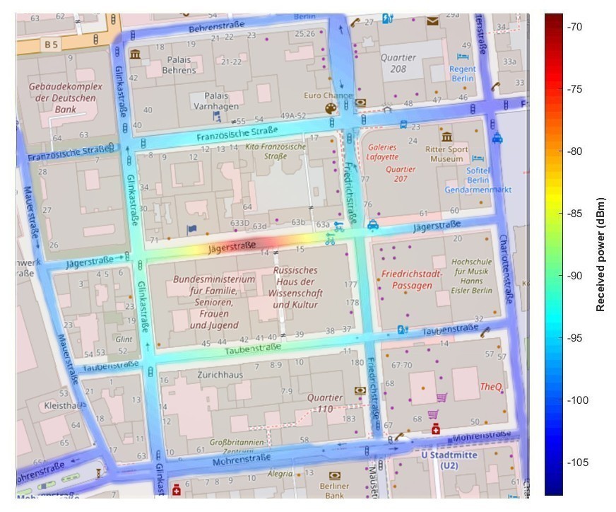
As mentioned before, our goal is to model the V2X environment as accurate as possible. Therefore, we use the $\mathrm{GEMV}^{2}$ model to obtain spatially consistent channels (cf. Section IV-C). We use OSM data from the center of Berlin, as shown in Fig.1 and we let SUMO generate random routes along the street grid for the specified simulation duration. The SUMO traces for each vehicle are imported into the $\mathrm{GEMV}^{2}$ based MATLAB simulator, which combines them with the geometric features from OSM to generate both V2V and V2I channels. This is additionally illustrated in Fig.1, where different colors indicate the received power generated by $\mathrm{GEMV}^{2}$ at all locations along the street grid with respect to an arbitrarily selected transmitter location.

The Q-network for each agent is a five-layer fully connected neural network that comprises 3 hidden layers, with rectified linear unit (ReLU)as the activation function. We also use the $\epsilon$-greedy strategy to balance between exploration and exploitation, and we use the RMSProp optimizer [11] to update network parameters for training. We train each agent’s Q-network in an episodic pattern. Each episode is spanning over the V2V payload delivery time $T$ and starts with a full V2V payload of size $B$. Thereby, the exploration rate $\epsilon$ is decreased linearly from $1$ to $0.02$ over the first $80\%$ of the episodes and remains constant afterward. During the training phase, we fix the large-scale fading for 100 training episodes and let the small-scale fading change over each time-step $t$. As in [1], we do this to support the agents in acquiring the underlying fading dynamics of the channel.

In the evaluation phase, however, the vehicles update their large-scale fading after every V2V payload delivery time $T$. Moreover, the values of $\epsilon$ and the iteration number $i$ are set to the values of the last step of the training phase. For a single simulation run, the traces and channels experienced by each vehicle are captured for 13 seconds, where the first 3 seconds are used for the training phase, and the remaining 10 seconds are used for the evaluation phase. The plots shown in this work are averaged over multiple simulation runs, where in each simulation run, the vehicles are assigned a new random SUMO trace (with a different starting position). The detailed simulation parameters can be found in Table I.

Figure 1: Simulation area in the center of Berlin. The colors indicate the receive powers with respect to an arbitrarily selected transmitter location. (© OpenStreetMap contributors)

TABLE I: Simulation parameters.

Parameter	Value
Carrier frequency $f_{c}$	2 GHz
Bandwidth W	4 MHz
Number of V2I links $M$	4
Number of V2V links $K$	4
V2I transmit power $P_{m}^{c}$	23 dBm
V2V transmit power $P_{k}^{d}$	[23,15,5,-100] dBm
V2V payload delivery time $T$	100 ms
Noise power $\sigma^{2}$	-114 dBm
V2V payload size $B$	[1,2,…] x 1060 bytes
Number of simulation runs	5

V-A Performance of Double DQN

In the following, we compare MARL based on DQN (as proposed in [1]) with the proposed DDQN approach, introduced in Section IV-A. In addition, we show the performance of the same random baseline as in [1], which selects transmission powers and spectrum sub-bands randomly. We train each agent’s Q-network for a total of $3000$ episodes.

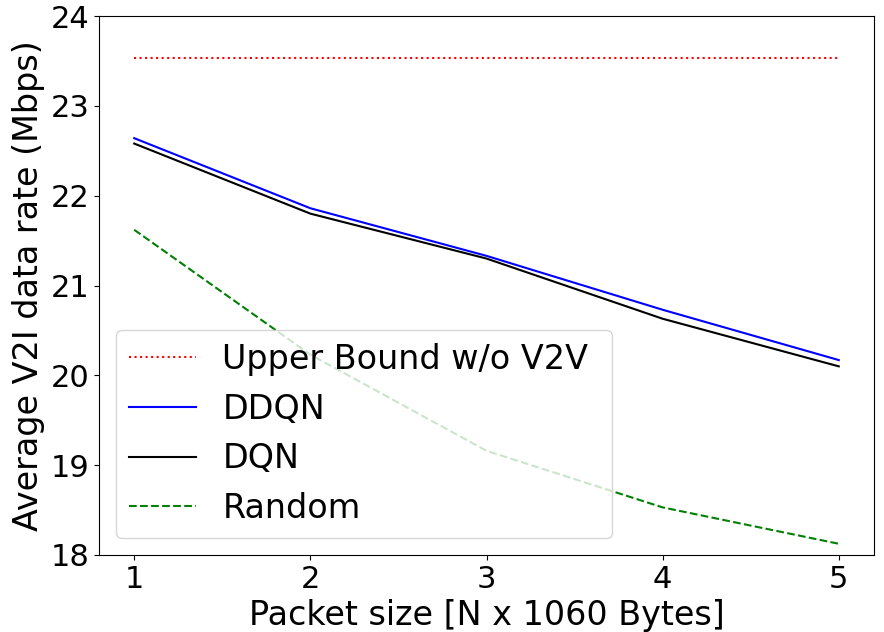
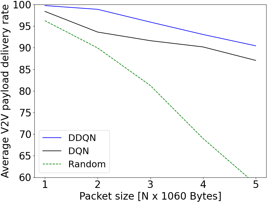
Fig.2 shows the V2I performance with increasing payload size $B$. At the end of the evaluation phases, average data rates of V2I links (shown in Fig.2) and the V2V payload delivery rate (shown in Fig.2) are computed. The increase of the V2V payload not only results in a longer V2V transmission duration, as it becomes more challenging to completely deliver the payload within the delivery time limit, but it also leads to an increased interference to V2I links. This in turn results in a reduced V2I sum capacity, as we can observe in Fig.2.

While the V2I performance for the DDQN approach is close to the DQN approach, we observe in Fig.2 that the proposed approach improves the success probability compared to the DQN approach by up to $4\%$. As expected, the success probability drops for higher payload sizes, where the random baseline method shows a much more severe degradation, compared to the reinforcement learning-based algorithms.

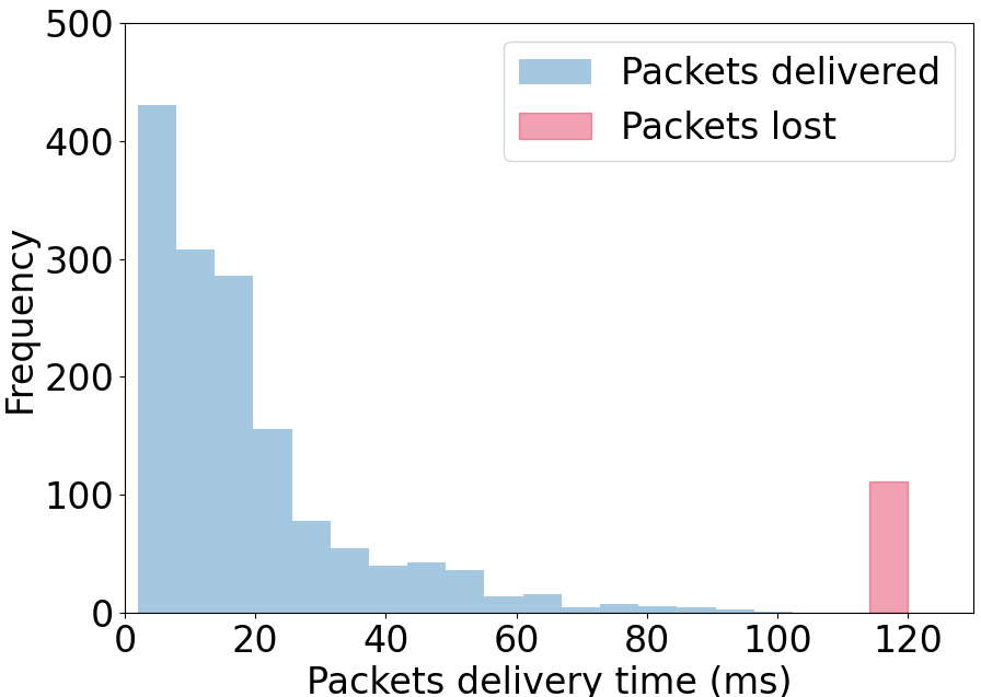
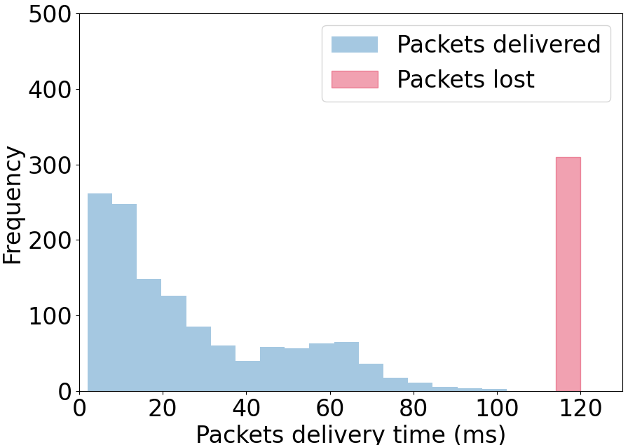
The design of the reward function encourages the agents to finish their V2V packet transmission in a timely manner. Fig.2 and Fig.2 show histograms of the observed packet delivery times for the proposed DDQN-based algorithm and the DQN-based baseline from [1], respectively. Here, we fix the payload size to $4\times 1060$ bytes, and all packets delivered after the packet delivery time limit (i.e, $T=100$ ms) are considered to be lost (accumulated in the red bars). Clearly, the DDQN approach leads to earlier completion of transmissions, which results in a significantly reduced number of failed packet deliveries. For the given simulation settings, the median packet delivery time for successful V2V transmission using DDQN is $14$ ms as compared to $19$ ms for DQN. In summary, the results indicate that the reduction in overestimation of Q-values due to the DDQN approach positively influences the learning for the agents.

(a) Sum capacity of V2I links.

(b) V2V delivery rate.

(c) Histogram of V2V packet delivery times for DDQN.

(d) Histogram of V2V packet delivery times for DQN.

Figure 2: Comparison of DDQN, DQN and random baseline over different payload sizes.

V-B Performance of Transfer Q-Learning

Subsequently, we evaluate the learning performance with, and without the prior knowledge of an expert model (as explained in Section IV-B). For this, we compare the same DDQN-based method, as evaluated in the previous subsection, with the proposed DDQN-TQL method. The state space, action space and reward function for both the expert model and the learner model are identical. To evaluate the adaptivity of DDQN-TQL, we use different channel conditions for the training of both models. The main motivation in using DDQN-TQL is to reduce the required training duration. To evaluate this, we reduce the training duration of the learner model to 1,800 episodes in our performance evaluations (while we keep the training duration of the expert model at 3,000 episodes).

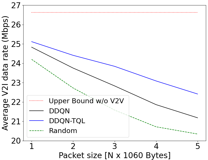
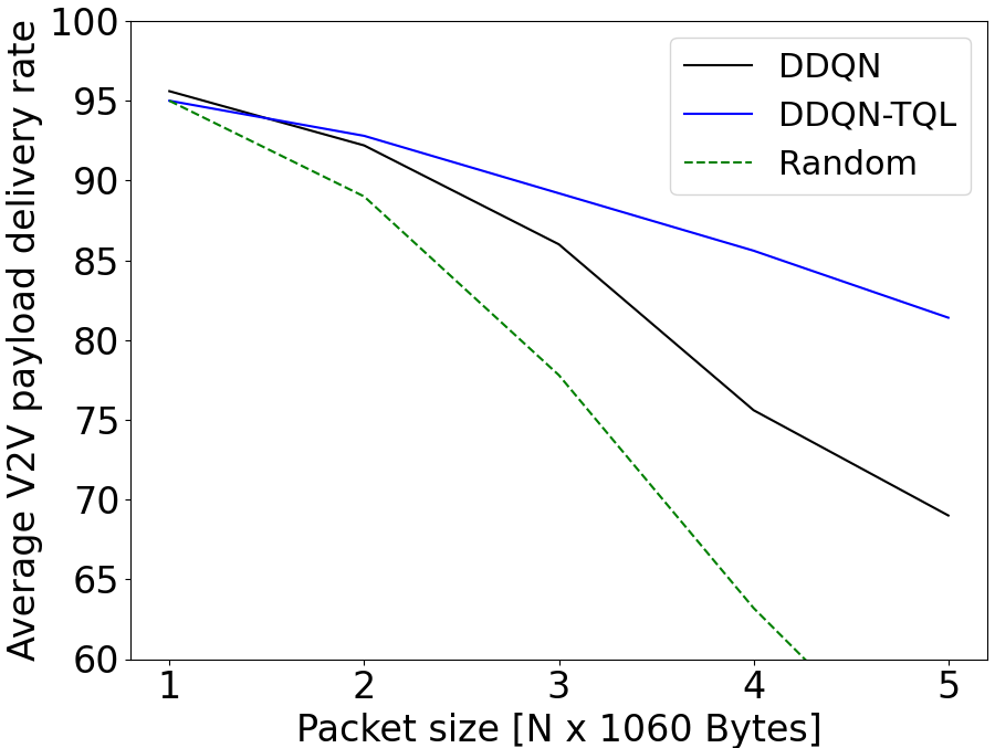
The experimental results in Fig.3, which shows the average sum capacity of V2I links, support this reasoning. We can observe that DDQN-TQL outperforms DDQN for all considered payload sizes. While for small payload sizes the performance differences are small, for high payload sizes, DDQN-TQL provides significant gains in terms of V2I data rates. In Fig.3, which shows the V2V payload delivery rate, we observe a similar behavior. Especially for large packet sizes, DDQN-TQL enables the agents to learn policies within the given training time that show significantly higher performance than the policies obtained without the Q-value transfer. For example, for a payload size of $4\times 1060$ bytes, we observe performance gains of $6\%$ and $12\%$, for the V2I sum capacity, and the V2V payload delivery rate, respectively.

(a) Sum capacity of V2I links.

(b) V2V delivery rate.

(c) Histogram of V2V packet delivery times for DDQN-TQL.

(d) Histogram of V2V packet delivery times for DDQN.

Figure 3: Comparison of DDQN-TQL, DDQN and random baseline over different payload sizes.

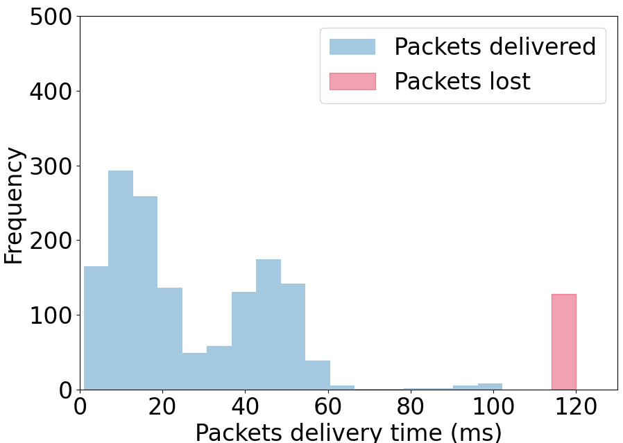
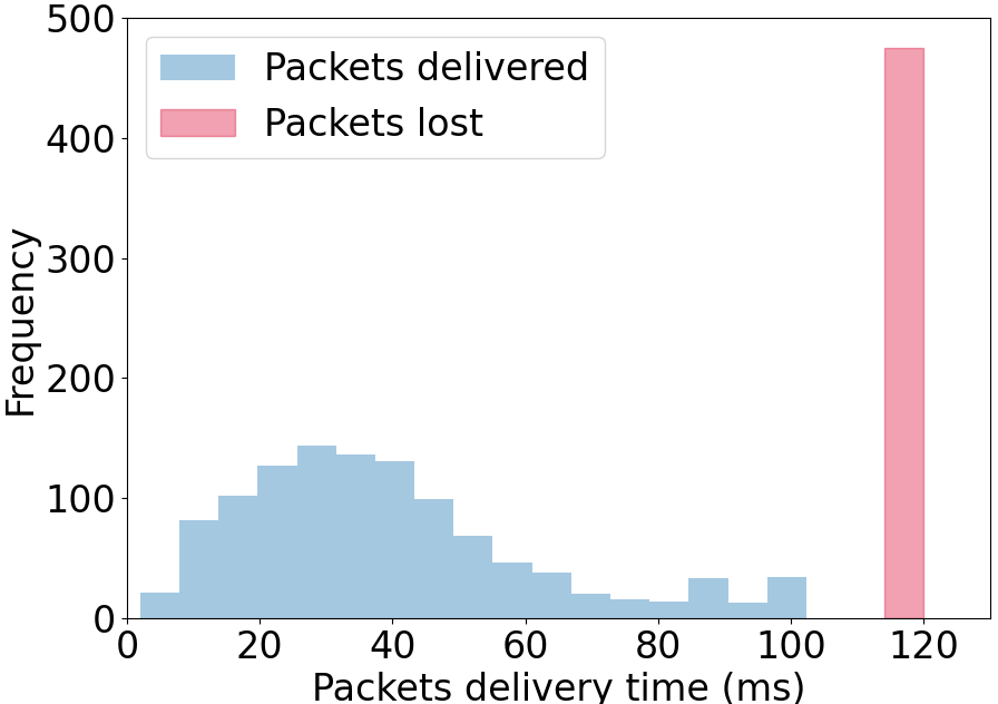
The packet delivery times for DDQN-TQL and DDQN are provided in greater detail in Fig.3 and Fig.3, respectively. Again, we fix the payload size to $4\times 1060$ bytes. The changes in the empirical distribution of the packet delivery times demonstrate the effectiveness of the knowledge transfer approach for the given training duration. The TQL-based approach leads to policies that finish transmissions earlier and thus reduce the number of failed packet deliveries. More precisely, for the simulations shown in Fig. 3, the median packet delivery time for successful V2V transmission using DDQN-TQL is $18$ ms, compared to $35$ ms for DDQN.

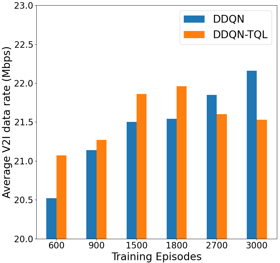
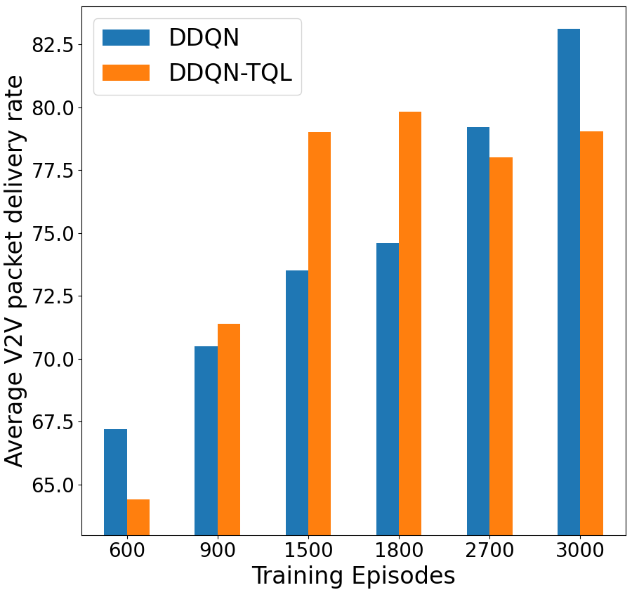
We would like to point out that the performance of the proposed method highly depends on the choice of the number of training episodes. For a very short training duration, agents are unable to properly explore the environment, and reinforcement learning-based schemes will not even outperform the random baseline. On the other hand, learning for very long training intervals can lead to a potential over-fitting, which is a common problem for deep RL algorithms [12][13]. As the TQL approach is more effected by over-fitting, simulations show that for larger numbers of training episodes it is outperformed by DDQN, where we train our model from scratch without any previous knowledge about input-output relations.

This behaviour is illustrated in Fig.4. The performance with respect to V2I (Fig.4) and V2V (Fig.4) links are shown for a fixed payload size of $4\times 1060$ bytes. The figure confirms the previous discussions, and we observe that especially in scenarios with only a reduced training time around $1800$ training episodes, the TQL approach provides significant advantages.

(a) Sum capacity of V2I links.

(b) V2V delivery rate.

Figure 4: Comparison of DDQN-TQL and DDQN for different numbers of training episodes.

VI Conclusion

In this paper, we proposed improvements and extensions to deep Q-learning-based approaches (such as the MARL algorithm in [1]) to distributed spectrum sharing in V2X communications. In particular, we proposed and evaluated solutions for reducing the overestimation of Q-values (using the Double DQN method), and for reducing the training time (using a transfer Q-learning approach). In contrast to previous studies, we evaluated the proposed methods using a realistic vehicular setting based on the geometry-based deterministic $\mathrm{GEMV}^{2}$ channel model. Simulations show that the use of DDQN indeed results in improved learning performance of the agents. Moreover, we observe that the performance of the proposed DDQN method with TQL is significantly less susceptible to a shorter training duration than without TQL.

References

- [1] L. Liang, H. Ye, and G. Y. Li, “Spectrum Sharing in Vehicular Networks Based on Multi-Agent Reinforcement Learning,” IEEE Journal on Selected Areas in Communications, vol. 37, no. 10, pp. 2282–2292, 2019.
- [2] H. Van Hasselt, A. Guez, and D. Silver, “Deep Reinforcement Learning with Double Q-learning,” in Proceedings of the AAAI Conference on Artificial Intelligence, vol. 30, no. 1, 2016.
- [3] M. Boban, J. Barros, and O. K. Tonguz, “Geometry-Based Vehicle-to-Vehicle Channel Modeling for Large-Scale Simulation,” IEEE Transactions on Vehicular Technology, vol. 63, no. 9, pp. 4146–4164, 2014.
- [4] “3rd Generation Partnership Project; Technical Specification Group Radio Access Network; Study on enhancement of 3GPP Support for 5G V2X Services; (Release 15),” 3GPP, TR 22.886, Mar. 2017, v 15.1.0.
- [5] C. J. Watkins and P. Dayan, “Q-learning,” Machine learning, vol. 8, no. 3-4, pp. 279–292, 1992.
- [6] R. S. Sutton and A. G. Barto, Reinforcement Learning: An Introduction. MIT press, 2018.
- [7] V. Mnih, K. Kavukcuoglu, D. Silver, A. A. Rusu, J. Veness, M. G. Bellemare, A. Graves, M. Riedmiller, A. K. Fidjeland, G. Ostrovski et al., “Human-Level Control through Deep Reinforcement Learning,” nature, vol. 518, no. 7540, pp. 529–533, 2015.
- [8] H. Hasselt, “Double Q-learning,” Advances in neural information processing systems, vol. 23, pp. 2613–2621, 2010.
- [9] P. A. Lopez, M. Behrisch, L. Bieker-Walz, J. Erdmann, Y.-P. Flötteröd, R. Hilbrich, L. Lücken, J. Rummel, P. Wagner, and E. Wießner, “Microscopic Traffic Simulation using SUMO,” in The 21st IEEE International Conference on Intelligent Transportation Systems. IEEE, 2018. [Online]. Available: https://elib.dlr.de/124092/
- [10] OpenStreetMap contributors, “Planet Dump Retrieved from https://planet.osm.org ,” https://www.openstreetmap.org , 2017.
- [11] S. Ruder, “An Overview of Gradient Descent Optimization Algorithms,” arXiv preprint arXiv:1609.04747, 2016.
- [12] M. Hardt, B. Recht, and Y. Singer, “Train Faster, Generalize Better: Stability of Stochastic Gradient Descent,” in International Conference on Machine Learning. PMLR, 2016, pp. 1225–1234.
- [13] C. Zhang, O. Vinyals, R. Munos, and S. Bengio, “A Study on Overfitting in Deep Reinforcement Learning,” arXiv preprint arXiv:1804.06893, 2018.