No Regrets for Learning the Prior in Bandits

Abstract

We propose $\tt AdaTS$, a Thompson sampling algorithm that adapts sequentially to bandit tasks that it interacts with. The key idea in $\tt AdaTS$ is to adapt to an unknown task prior distribution by maintaining a distribution over its parameters. When solving a bandit task, that uncertainty is marginalized out and properly accounted for. $\tt AdaTS$ is a fully-Bayesian algorithm that can be implemented efficiently in several classes of bandit problems. We derive upper bounds on its Bayes regret that quantify the loss due to not knowing the task prior, and show that it is small. Our theory is supported by experiments, where $\tt AdaTS$ outperforms prior algorithms and works well even in challenging real-world problems.

1 Introduction

We study the problem of maximizing the total reward, or minimizing the total regret, in a sequence of stochastic bandit instances [29, 4, 31]. We consider a Bayesian version of the problem, where the bandit instances are drawn from some distribution. More specifically, the learning agent interacts with $m$ bandit instances in $m$ tasks, with one instance per task. The interaction with each task is for $n$ rounds and with $K$ arms. The reward distribution of arm $i\in[K]$ in task $s\in[m]$ is $p_{i}(\cdot;\theta_{s,*})$, where $\theta_{s,*}$ is a shared parameter of all arms in task $s$. When arm $i$ is pulled in task $s$, the agent receives a random reward from $p_{i}(\cdot;\theta_{s,*})$. The parameters $\theta_{1,*},\dots,\theta_{m,*}$ are drawn independently of each other from a task prior $P(\cdot;\mu_{*})$. The task prior is parameterized by an unknown meta-parameter $\mu_{*}$, which is drawn from a meta-prior $Q$. The agent does not know $\mu_{*}$ or $\theta_{1,*},\dots,\theta_{m,*}$. However, it knows $Q$ and the parametric forms of all distributions, which help it to learn about $\mu_{*}$. This is a form of meta-learning [39, 40, 7, 8], where the agent learns to act from interactions with bandit instances.

A simple approach is to ignore the hierarchical structure of the problem and solve each bandit task independently with some bandit algorithm, such as Thompson sampling (TS) [38, 11, 2, 37]. This may be highly suboptimal. To illustrate this, imagine that arm $1$ is optimal for any $\theta$ in the support of $P(\cdot;\mu_{*})$. If $\mu_{*}$ was known, any reasonable algorithm would only pull arm $1$ and have zero regret over any horizon. Likewise, a clever algorithm that learns $\mu_{*}$ should eventually pull arm $1$ most of the time, and thus have diminishing regret as it interacts with a growing number of tasks. Two challenges arise when designing the clever algorithm. First, can it be computationally efficient? Second, what is the regret due to adapting to $\mu_{*}$?

We make the following contributions. First, we propose a Thompson sampling algorithm for our problem, which we call $\tt AdaTS$. $\tt AdaTS$ maintains a distribution over the meta-parameter $\mu_{*}$, which concentrates over time and is marginalized out when interacting with individual bandit instances. Second, we propose computationally-efficient implementations of $\tt AdaTS$ for multi-armed bandits [29, 4], linear bandits [14, 1], and combinatorial semi-bandits [19, 13, 26]. These implementations are for specific reward distributions and conjugate task priors. Third, we bound the $n$-round Bayes regret of $\tt AdaTS$ in linear bandits and semi-bandits, and multi-armed bandits as a special case. The Bayes regret is defined by taking an expectation over all random quantities, including $\mu_{*}\sim Q$. Our bounds show that not knowing $\mu_{*}$ has a minimal impact on the regret as the number of tasks grows, of only $\tilde{O}(\sqrt{mn})$. This is in a sharp contrast to prior work [28], where this is $\tilde{O}(\sqrt{m}n^{2})$. Finally, our experiments show that $\tt AdaTS$ quickly adapts to the unknown meta-parameter $\mu_{*}$, is robust to meta-prior misspecification, and performs well even in challenging classification problems.

We present a general framework for learning to explore from similar past exploration problems. One potential application is cold-start personalization in recommender systems where users are tasks. The users have similar preferences, but neither the individual preferences nor their similarity is known in advance. Another application could be online regression with bandit feedback (Section E.2) where individual regression problems are tasks. Similar examples in the tasks have similar mean responses, which are unknown in advance.

2 Setting

We first introduce our notation. The set $\left\{1,\dots,n\right\}$ is denoted by $[n]$. The indicator $\mathds{1}\!\left\{E\right\}$ denotes that event $E$ occurs. The $i$-th entry of vector $v$ is $v_{i}$. If the vector or its index are already subindexed, we write $v(i)$. We use $\tilde{O}$ for the big-O notation up to polylogarithmic factors. A diagonal matrix with entries $v$ is denoted $\mathrm{diag}\left(v\right)$. We use the terms arm and action interchangeably, depending on the context.

Figure 1: Graphical model of our environment.

Our setting was proposed in Kveton et al. [28] and is defined as follows. Each bandit problem instance has $K$ arms. Each arm $i\in[K]$ is defined by distribution $p_{i}(\cdot;\theta)$ with parameter $\theta\in\Theta$. The parameter $\theta$ is shared among all arms. The mean of $p_{i}(\cdot;\theta)$ is denoted by $r(i;\theta)$. The learning agent interacts with $m$ instances, one at each of $m$ tasks. At the beginning of task $s\in[m]$, an instance $\theta_{s,*}\in\Theta$ is sampled i.i.d. from a task prior $P(\cdot;\mu_{*})$, which is parameterized by $\mu_{*}$. The agent interacts with $\theta_{s,*}$ for $n$ rounds. In round $t\in[n]$, it pulls one arm and observes a stochastic realization of its reward. We denote the pulled arm in round $t$ of task $s$ by $A_{s,t}\in[K]$, the realized rewards of all arms in round $t$ of task $s$ by $Y_{s,t}\in\mathbb{R}^{K}$, and the reward of arm $i\in[K]$ by $Y_{s,t}(i)\sim p_{i}(\cdot;\theta_{s,*})$. We assume that the realized rewards $Y_{s,t}$ are i.i.d. with respect to both $s$ and $t$. A graphical model of our environment is drawn in Figure 1. We define the distribution-specific parameters $\mu_{q}$, $\Sigma_{q}$, $\Sigma_{0}$, and $\sigma^{2}$ when we instantiate our framework. Our terminology is summarized in Appendix A.

The $n$-round regret of an agent or algorithm over $m$ tasks with task prior $P(\cdot;\mu_{*})$ is defined as

$$R(m,n;\mu_{*})=\sum_{s=1}^{m}\mathbb{E}\left[\sum_{t=1}^{n}r(A_{s,*};\theta_{s,*})-r(A_{s,t};\theta_{s,*})\,\middle|\,\mu_{*}\right]\,,$$ (1)

where $A_{s,*}=\operatorname*{arg\,max\,}_{i\in[K]}r(i;\theta_{s,*})$ is the optimal arm in the random problem instance $\theta_{s,*}$ in task $s\in[m]$. The above expectation is over problem instances $\theta_{s,*}\sim P(\cdot;\mu_{*})$, their realized rewards, and also pulled arms. Note that $\mu_{*}$ is fixed. Russo and Van Roy [36] showed that the Bayes regret, which matches the definition in (1) in any task, of Thompson sampling in a $K$-armed bandit with $n$ rounds is $\tilde{O}(\sqrt{Kn})$. So, when TS is applied independently in each task, $R(m,n;\mu_{*})=\tilde{O}(m\sqrt{Kn})$.

Our goal is to attain a comparable regret without knowing $\mu_{*}$. We frame this problem in a Bayesian fashion, where $\mu_{*}\sim Q$ before the learning agent interacts with the first task. The agent knows $Q$ and we call it a meta-prior. Accordingly, we consider $R(m,n)=\mathbb{E}\left[R(m,n;\mu_{*})\right]$ as a metric and call it the Bayes regret. Our approach is motivated by hierarchical Bayesian models [20], where the uncertainty in prior parameters, such as $\mu_{*}$, is represented by another distribution, such as $Q$. In these models, $Q$ is called a hyper-prior and $\mu_{*}$ is called a hyper-parameter. We attempt to learn $\mu_{*}$ from sequential interactions with instances $\theta_{s,*}\sim P(\cdot;\mu_{*})$, which are also unknown. The agent can only observe their noisy realizations $Y_{s,t}$.

3 Algorithm

Our algorithm is presented in this section. To describe it, we need to introduce several notions of history, the past interactions of the agent. We denote by $H_{s}=(A_{s,t},Y_{s,t}(A_{s,t}))_{t=1}^{n}$ the history in task $s$ and by $H_{1:s}=H_{1}\oplus\dots\oplus H_{s}$ a concatenated vector of all histories in the first $s$ tasks. The history up to round $t$ in task $s$ is $H_{s,t}=(A_{s,\ell},Y_{s,\ell}(A_{s,\ell}))_{\ell=1}^{t-1}$ and all history up to round $t$ in task $s$ is $H_{1:s,t}=H_{1:s-1}\oplus H_{s,t}$. We denote the conditional probability distribution given history $H_{1:s,t}$ by $\mathbb{P}_{s,t}(\cdot)=\mathbb{P}\left(\cdot\,\middle|\,H_{1:s,t}\right)$ and the corresponding conditional expectation by $\mathbb{E}_{s,t}[\cdot]=\mathbb{E}\left[\cdot\,\middle|\,H_{1:s,t}\right]$.

Our algorithm is a form of Thompson sampling [38, 11, 2, 37]. TS pulls arms proportionally to being optimal with respect to the posterior. In particular, let $\mathcal{L}_{s,t}(\theta)=\prod_{\ell=1}^{t-1}p_{A_{s,\ell}}(Y_{s,\ell}(A_{s,\ell});\theta)$ be the likelihood of observations in task $s$ up to round $t$. If the prior $P(\cdot;\mu_{*})$ was known, the posterior of instance $\theta$ in round $t$ would be $P_{s,t}^{\textsc{ts}}(\theta)\propto\mathcal{L}_{s,t}(\theta)\,P(\theta;\mu_{*})$. TS would sample $\tilde{\theta}_{t}\sim P_{s,t}^{\textsc{ts}}$ and pull arm $A_{t}=\operatorname*{arg\,max\,}_{i\in[K]}r(i;\tilde{\theta}_{t})$.

We address the case of unknown $\mu_{*}$. The key idea in our method is to maintain a posterior density of $\mu_{*}$, which we call a meta-posterior. This density represents uncertainty in $\mu_{*}$ given history. In task $s$, we denote it by $Q_{s}$ and define it such that $\mathbb{P}\left(\mu_{*}\in B\,\middle|\,H_{1:s-1}\right)=\int_{\mu\in B}Q_{s}(\mu)\,d\kappa_{1}(\mu)$ holds for any set $B$, where $\kappa_{1}$ is the reference measure for $\mu$. We use this more general notation, as opposing to $d\mu$, because $\mu$ can be both continuous and discrete. When solving task $s$, $Q_{s}$ is used to compute an uncertainty-adjusted task prior $P_{s}$, which is a posterior density of $\theta_{s,*}$ given history. Formally, $P_{s}$ is a density such that $\mathbb{P}\left(\theta_{s,*}\in B\,\middle|\,H_{1:s-1}\right)=\int_{\theta\in B}P_{s}(\theta)\,d\kappa_{2}(\theta)$ holds for any set $B$, where $\kappa_{2}$ is the reference measure for $\theta$. After computing $P_{s}$, we run TS with prior $P_{s}$ to solve task $s$. To maintain $Q_{s}$ and $P_{s}$, we find it useful expressing them using a recursive update rule below.

[]propositionposterior Let $\mathcal{L}_{s}(\theta)=\prod_{\ell=1}^{n}p_{A_{s,\ell}}(Y_{s,\ell}(A_{s,\ell});\theta)$ be the likelihood of observations in task $s$. Then for any task $s\in[m]$,

$$P_{s}(\theta)=\int_{\mu}P(\theta;\mu)\,Q_{s}(\mu)\,d\kappa_{1}(\mu)\,,\quad Q_{s}(\mu)=\int_{\theta}\mathcal{L}_{s-1}(\theta)\,P(\theta;\mu)\,d\kappa_{2}(\theta)\,Q_{s-1}(\mu)\,.$$

The claim is proved in Appendix A. The proof uses the Bayes rule, where we carefully account for the fact that the observations are collected adaptively, the pulled arm in round $t$ of task $s$ depends on history $H_{1:s,t}$. The pseudocode of our algorithm is in Algorithm 1. Since the algorithm adapts to the unknown task prior $P(\cdot;\mu_{*})$, we call it $\tt AdaTS$. $\tt AdaTS$ can be implemented efficiently when $P_{s}$ is a conjugate prior for rewards, or a mixture of conjugate priors. We discuss several exact and efficient implementations starting from Section 3.1.

Algorithm 1 $\tt AdaTS$: Instance-adaptive exploration in Thompson sampling.

1:Initialize meta-prior $Q_{0}\leftarrow Q$

2:for $s=1,\dots,m$ do

3:     Compute meta-posterior $Q_{s}$ (Section 3)

4:     Compute uncertainty-adjusted task prior $P_{s}$ (Section 3)

5:     for $t=1,\dots,n$ do

6:         Compute posterior of $\theta$ in task $s$, $P_{s,t}(\theta)\propto\mathcal{L}_{s,t}(\theta)P_{s}(\theta)$

7:         Sample $\tilde{\theta}_{s,t}\sim P_{s,t}$, pull arm $A_{s,t}\leftarrow\operatorname*{arg\,max\,}_{i\in[K]}r(i;\tilde{\theta}_{s,t})$, and observe $Y_{s,t}(A_{s,t})$      

The design of $\tt AdaTS$ is motivated by $\tt MetaTS$ [28], which also maintains a meta-posterior $Q_{s}$. The difference is that $\tt MetaTS$ samples $\tilde{\mu}_{s}\sim Q_{s}$ in task $s$ to be optimistic with respect to the unknown $\mu_{*}$. Then it runs TS with prior $P(\cdot;\tilde{\mu}_{s})$. While simple and intuitive, the sampling of $\tilde{\mu}_{s}$ induces a high variance and leads to a conservative worst-case analysis. We improve $\tt MetaTS$ by avoiding the sampling step. This leads to tighter and more general regret bounds (Section 4), beyond multi-armed bandits; while the practical performance also improves significantly (Section 5).

3.1 Gaussian Bandit

We start with a $K$-armed Gaussian bandit with mean arm rewards $\theta\in\mathbb{R}^{K}$. The reward distribution of arm $i$ is $p_{i}(\cdot;\theta)=\mathcal{N}(\cdot;\theta_{i},\sigma^{2})$, where $\sigma>0$ is reward noise and $\theta_{i}$ is the mean reward of arm $i$. A natural conjugate prior for this problem class is $P(\cdot;\mu)=\mathcal{N}(\cdot;\mu,\Sigma_{0})$, where $\Sigma_{0}=\mathrm{diag}\left((\sigma_{0,i}^{2})_{i=1}^{K}\right)$ is known and we learn $\mu\in\mathbb{R}^{K}$.

Because the prior is a multivariate Gaussian, $\tt AdaTS$ can be implemented efficiently with a Gaussian meta-prior $Q(\cdot)=\mathcal{N}(\cdot;\mu_{q},\Sigma_{q})$, where $\mu_{q}=(\mu_{q,i})_{i=1}^{K}$ and $\Sigma_{q}=\mathrm{diag}\left((\sigma_{q,i}^{2})_{i=1}^{K}\right)$ are known mean parameter vector and covariance matrix, respectively. In this case, the meta-posterior in task $s$ is also a Gaussian $Q_{s}(\cdot)=\mathcal{N}(\cdot;\hat{\mu}_{s},\hat{\Sigma}_{s})$, where $\hat{\mu}_{s}=(\hat{\mu}_{s,i})_{i=1}^{K}$ and $\hat{\Sigma}_{s}=\mathrm{diag}\left((\hat{\sigma}_{s,i}^{2})_{i=1}^{K}\right)$ are defined as

$$\hat{\mu}_{s,i}=\hat{\sigma}_{s,i}^{2}\left(\frac{\mu_{q,i}}{\sigma_{q,i}^{2}}+\sum_{\ell=1}^{s-1}\frac{T_{\ell,i}}{T_{\ell,i}\,\sigma_{0,i}^{2}+\sigma^{2}}\frac{B_{\ell,i}}{T_{\ell,i}}\right)\,,\quad\hat{\sigma}_{s,i}^{-2}=\sigma_{q,i}^{-2}+\sum_{\ell=1}^{s-1}\frac{T_{\ell,i}}{T_{\ell,i}\,\sigma_{0,i}^{2}+\sigma^{2}}\,.$$ (2)

Here $T_{\ell,i}=\sum_{t=1}^{n}\mathds{1}\!\left\{A_{\ell,t}=i\right\}$ is the number of pulls of arm $i$ in task $\ell$ and the total reward from these pulls is $B_{\ell,i}=\sum_{t=1}^{n}\mathds{1}\!\left\{A_{\ell,t}=i\right\}Y_{\ell,t}(i)$. The above formula has a very nice interpretation. The posterior mean $\hat{\mu}_{s,i}$ of the meta-parameter of arm $i$ is a weighted sum of the noisy estimates of the means of arm $i$ from the past tasks $B_{\ell,i}/T_{\ell,i}$ and the prior. In this sum, each bandit task is essentially a single observation. The weights are proportional to the number of pulls in a task, giving the task with more pulls a higher weight. They vary from $(\sigma_{0,i}^{2}+\sigma^{2})^{-1}$, when the arm is pulled only once, up to $\sigma_{0,i}^{-2}$. This is the minimum amount of uncertainty that cannot be reduced by more pulls.

The update in (2) is by Lemma 1 in Appendix A, which we borrow from Kveton et al. [28]. From Section 3, we have that the uncertainty-adjusted prior for task $s$ is $P_{s}(\cdot)=\mathcal{N}(\cdot;\hat{\mu}_{s},\hat{\Sigma}_{s}+\Sigma_{0})$.

3.2 Linear Bandit with Gaussian Rewards

Now we generalize Section 3.1 and consider a linear bandit [14, 1] with $K$ arms and $d$ dimensions. Let $\mathcal{A}\subset\mathbb{R}^{d}$ be an action set such that $\left|\mathcal{A}\right|=K$. We refer to each $a\in\mathcal{A}$ as an arm. Then, with a slight abuse of notation from Section 2, the reward distribution of arm $a$ is $p_{a}(\cdot;\theta)=\mathcal{N}(\cdot;a^{\top}\theta,\sigma^{2})$, where $\theta\in\mathbb{R}^{d}$ is shared by all arms and $\sigma>0$ is reward noise. A conjugate prior for this problem class is $P(\cdot;\mu)=\mathcal{N}(\cdot;\mu,\Sigma_{0})$, where $\Sigma_{0}\in\mathbb{R}^{d\times d}$ is known and we learn $\mu\in\mathbb{R}^{d}$.

As in Section 3.1, $\tt AdaTS$ can be implemented efficiently with a meta-prior $Q(\cdot)=\mathcal{N}(\cdot;\mu_{q},\Sigma_{q})$, where $\mu_{q}\in\mathbb{R}^{d}$ is a known mean parameter vector and $\Sigma_{q}\in\mathbb{R}^{d\times d}$ is a known covariance matrix. In this case, $Q_{s}(\cdot)=\mathcal{N}(\cdot;\hat{\mu}_{s},\hat{\Sigma}_{s})$, where

$$\hat{\mu}_{s} =\hat{\Sigma}_{s}\left(\Sigma_{q}^{-1}\mu_{q}+\sum_{\ell=1}^{s-1}\frac{B_{\ell}}{\sigma^{2}}-\frac{G_{\ell}}{\sigma^{2}}\left(\Sigma_{0}^{-1}+\frac{G_{\ell}}{\sigma^{2}}\right)^{-1}\frac{B_{\ell}}{\sigma^{2}}\right)\,,$$

$$\hat{\Sigma}_{s}^{-1} =\Sigma_{q}^{-1}+\sum_{\ell=1}^{s-1}\frac{G_{\ell}}{\sigma^{2}}-\frac{G_{\ell}}{\sigma^{2}}\left(\Sigma_{0}^{-1}+\frac{G_{\ell}}{\sigma^{2}}\right)^{-1}\frac{G_{\ell}}{\sigma^{2}}\,.$$

Here $G_{\ell}=\sum_{t=1}^{n}A_{\ell,t}A_{\ell,t}^{\top}$ is the outer product of the feature vectors of the pulled arms in task $\ell$ and $B_{\ell}=\sum_{t=1}^{n}A_{\ell,t}Y_{\ell,t}(A_{\ell,t})$ is their sum weighted by their rewards. The above update follows from Lemma 1 in Appendix A, which is due to Kveton et al. [28]. From Section 3, the uncertainty-adjusted prior for task $s$ is $P_{s}(\cdot)=\mathcal{N}(\cdot;\hat{\mu}_{s},\hat{\Sigma}_{s}+\Sigma_{0})$.

We note in passing that when $K=d$ and $\mathcal{A}$ is the standard Euclidean basis of $\mathbb{R}^{d}$, the linear bandit reduces to a $K$-armed bandit. Since the covariance matrices are unrestricted here, the formulation in this section also shows how to generalize Section 3.1 to arbitrary covariance matrices.

3.3 Semi-Bandit with Gaussian Rewards

A stochastic combinatorial semi-bandit [19, 12, 25, 26, 42], or semi-bandit for short, is a $K$-armed bandit where at most $L\leq K$ arms are pulled in each round. After the arms are pulled, the agent observes their individual rewards and its reward is the sum of the individual rewards. Semi-bandits can be used to solve online combinatorial problems, such as learning to route.

We consider a Gaussian reward distribution for each arm, as in Section 3.1. The difference in the semi-bandit formulation is that the action set is $\mathcal{A}\subseteq\Pi_{L}(K)$, where $\Pi_{L}(K)$ is the set of all subsets of $[K]$ of size at most $L$. In round $t$ of task $s$, the agents pulls arms $A_{s,t}\in\mathcal{A}$. The meta-posterior is updated analogously to Section 3.1. The only difference is that $\mathds{1}\!\left\{A_{\ell,t}=i\right\}$ becomes $\mathds{1}\!\left\{i\in A_{\ell,t}\right\}$.

3.4 Exponential-Family Bandit with Mixture Priors

We consider a general $K$-armed bandit with mean arm rewards $\theta\in\mathbb{R}^{K}$. The reward distribution of arm $i$ is any one-dimensional exponential-family distribution parameterized by $\theta_{i}$. In a Bernoulli bandit, this would be $p_{i}(\cdot;\theta)=\mathrm{Ber}(\cdot;\theta_{i})$. A natural prior for this reward model would be a product of per-arm conjugate priors, such as the product of betas for Bernoulli rewards.

It is challenging to generalize our approach beyond Gaussian models because we require more than the standard notion of conjugacy. Specifically, to apply $\tt AdaTS$ to an exponentially-family prior, such as the product of betas, we need a computationally tractable prior for that prior. In this case, it does not exist. We circumvent this issue by discretization. More specifically, let $\left\{P(\cdot;j)\right\}_{j=1}^{L}$ be a set of $L$ potential conjugate priors, where each $P(\cdot;j)$ is a product of one-dimensional exponential-family priors. Then a suitable meta-prior is a vector of initial beliefs into each potential prior. In particular, it is $Q(\cdot)=\mathrm{Cat}(\cdot;w_{q})$, where $w_{q}\in\Delta_{L-1}$ is the belief and $\Delta_{L}$ is the $L$-simplex.

In this case, $Q_{s}(j)=\int_{\theta}\mathcal{L}_{s-1}(\theta)P(\theta;j)\,d\kappa_{2}(\theta)\,Q_{s-1}(j)$ in Section 3 has a closed form, since it is a standard conjugate posterior update for a distribution over $\theta$ followed by integrating out $\theta$. In addition, $P_{s}(\theta)=\sum_{j=1}^{L}Q_{s}(j)P(\theta;j)$ is a mixture of exponential-family priors over $\theta$. This is an instance of latent bandits [22]. For these problems, Thompson sampling can be implemented exactly and efficiently. We do not analyze this setting because prior-dependent Bayes regret bounds for this problem class do not exist yet.

4 Regret Bounds

We first introduce common notation used in our proofs. The action set $\mathcal{A}\subseteq\mathbb{R}^{d}$ is fixed. Recall that a matrix $X\in\mathbb{R}^{d\times d}$ is positive semi-definite (PSD) if it is symmetric and its smallest eigenvalue is non-negative. For such $X$, we define $\sigma^{2}_{\max}(X)=\max_{a\in\mathcal{A}}a^{\top}Xa$. Although $\sigma^{2}_{\max}(X)$ depends on $\mathcal{A}$, we suppress this dependence because $\mathcal{A}$ is fixed. We denote by $\lambda_{1}(X)$ the maximum eigenvalue of $X$ and by $\lambda_{d}(X)$ the minimum eigenvalue of $X$.

We also need basic quantities from information theory. For two probability measures $P$ and $Q$ over a common measurable space, we use $D(P||Q)$ to denote the relative entropy of $P$ with respect to $Q$. It is defined as $D(P||Q)=\int\log(\frac{dP}{dQ})\,dP$, where $dP/dQ$ is the Radon-Nikodym derivative of $P$ with respect to $Q$; and is infinite when $P$ is not absolutely continuous with respect to $Q$. We slightly abuse our notation and let $P(X)$ denote the probability distribution of random variable $X$, $P(X\in\cdot)$. For jointly distributed random variables $X$ and $Y$, we let $P(X\mid Y)$ be the conditional distribution of $X$ given $Y$, $P(X\in\cdot\mid Y)$, which is $Y$-measurable and depends on random $Y$. The mutual information between $X$ and $Y$ is $I(X;Y)=D(P(X,Y)||P(X)P(Y))$, where $P(X)P(Y)$ is the distribution of the product of $P(X)$ and $P(Y)$. Intuitively, $I(X;Y)$ measures the amount of information that either $X$ or $Y$ provides about the other variable. For jointly distributed $X$, $Y$, and $Z$, we also need the conditional mutual information between $X$ and $Y$ conditioned on $Z$. We define this quantity as $I(X;Y\mid Z)=\mathbb{E}[\hat{I}(X;Y\mid Z)]$, where $\hat{I}(X;Y\mid Z)=D(P(X,Y\mid Z)||P(X\mid Z)P(Y\mid Z))$ is the random conditional mutual information between $X$ and $Y$ given $Z$. Note that $\hat{I}(X;Y\mid Z)$ is a function of $Z$. By the chain rule for the random conditional mutual information, $\hat{I}(X;Y_{1},Y_{2}\mid Z)=\mathbb{E}[\hat{I}(X;Y_{1}\mid Y_{2},Z)\mid Z]+\hat{I}(X;Y_{2}\mid Z)$, where expectation is over $Y_{2}\mid Z$. We would get the usual chain rule $I(X;Y_{1},Y_{2})=I(X;Y_{1}\mid Y_{2})+I(X;Y_{2})$ without $Z$.

4.1 Generic Regret Bound

We start with a generic adaptation of the analysis of Lu and Van Roy [33] to our setting. In round $t$ of task $s$, we denote the pulled arm by $A_{s,t}$, its observed reward by $Y_{s,t}\sim p_{A_{s,t}}(\cdot;\theta_{s,*})$, and the suboptimality gap by $\Delta_{s,t}=r(A_{s,*};\theta_{s,*})-r(A_{s,t};\theta_{s,*})$. For random variables $X$ and $Y$, we denote by $I_{s,t}(X;Y)=\hat{I}(X;Y\mid H_{1:s,t})$ the random mutual information between $X$ and $Y$ given history $H_{1:s,t}$ of all observations from the first $s-1$ tasks and the first $t-1$ rounds of task $s$. Similarly, for random variables $X$, $Y$, and $Z$, we denote by $I_{s,t}(X;Y\mid Z)=\mathbb{E}[\hat{I}(X;Y\mid Z,H_{1:s,t})\mid H_{1:s,t}]$ the random mutual information between $X$ and $Y$ conditioned on $Z$, given history $H_{1:s,t}$. It is helpful to think of $I_{s,t}$ as the conditional mutual information of $X\mid H_{1:s,t}$, $Y\mid H_{1:s,t}$, and $Z\mid H_{1:s,t}$.

Let $\Gamma_{s,t}$ and $\epsilon_{s,t}$ be potentially history-dependent non-negative random variables such that

$$\mathbb{E}_{s,t}[\Delta_{s,t}]\leq\Gamma_{s,t}\sqrt{I_{s,t}(\theta_{s,*};A_{s,t},Y_{s,t})}+\epsilon_{s,t}$$ (3)

holds almost surely. We want to keep both $\Gamma_{s,t}$ and $\epsilon_{s,t}$ small. The following lemma provides a bound on the total regret over $n$ rounds in each of $m$ tasks in terms of $\Gamma_{s,t}$ and $\epsilon_{s,t}$.

[]lemmadecomp Suppose that (3) holds for all $s\in[m]$ and $t\in[n]$, for some $\Gamma_{s,t},\epsilon_{s,t}\geq 0$. In addition, let $(\Gamma_{s})_{s\in[m]}$ and $\Gamma$ be non-negative constants such that $\Gamma_{s,t}\leq\Gamma_{s}\leq\Gamma$ holds for all $s\in[m]$ and $t\in[n]$ almost surely. Then

$$R(m,n)\leq\Gamma\sqrt{mnI(\mu_{*};H_{1:m})}+\sum_{s=1}^{m}\Gamma_{s}\sqrt{nI(\theta_{s,*};H_{s}\mid\mu_{*},H_{1:s-1})}+\sum_{s=1}^{m}\sum_{t=1}^{n}\mathbb{E}\left[\epsilon_{s,t}\right]\,.$$

The first term above is the price for learning $\mu_{*}$, while the second is the price for learning all $\theta_{s,*}$ when $\mu_{*}$ is known. Accordingly, the price for learning $\mu_{*}$ is negligible when the mutual information terms grow slowly with $m$ and $n$. Specifically, we show shortly in linear bandits that $\Gamma_{s,t}$ and $\epsilon_{s,t}$ can be set so that the last term of the bound is comparable to the rest, while $\Gamma_{s,t}$ grows slowly with $m$ and $n$. At the same time, $I(\mu_{*};H_{1:m})$ and $I(\theta_{s,*};H_{s}\mid\mu_{*},H_{1:s-1})$ are only logarithmic in $m$ and $n$. Thus the price for learning $\mu_{*}$ is $\tilde{O}(\sqrt{mn})$ while that for learning all $\theta_{s,*}$ is $\tilde{O}(m\sqrt{n})$. Now we are ready to prove Section 4.1.

Proof.

First, we use the chain rule of random conditional mutual information and derive

$$I_{s,t}(\theta_{s,*};A_{s,t},Y_{s,t})\leq I_{s,t}(\theta_{s,*},\mu_{*};A_{s,t},Y_{s,t})=I_{s,t}(\mu_{*};A_{s,t},Y_{s,t})+I_{s,t}(\theta_{s,*};A_{s,t},Y_{s,t}\mid\mu_{*})\,.$$

Now we take the square root of both sides, apply $\sqrt{a+b}\leq\sqrt{a}+\sqrt{b}$ to the right-hand side, and multiply both sides by $\Gamma_{s,t}$. This yields

$$\Gamma_{s,t}\sqrt{I_{s,t}(\theta_{s,*};A_{s,t},Y_{s,t})}\leq\Gamma_{s,t}\sqrt{I_{s,t}(\mu_{*};A_{s,t},Y_{s,t})}+\Gamma_{s,t}\sqrt{I_{s,t}(\theta_{s,*};A_{s,t},Y_{s,t}\mid\mu_{*})}\,.$$ (4)

We start with the second term in (4). Fix task $s$. From $\Gamma_{s,t}\leq\Gamma_{s}$, followed by the Cauchy-Schwarz and Jensen’s inequalities, we have

$$\mathbb{E}\left[\sum_{t=1}^{n}\Gamma_{s,t}\sqrt{I_{s,t}(\theta_{s,*};A_{s,t},Y_{s,t}\mid\mu_{*})}\right] \leq\Gamma_{s}\sqrt{n\mathbb{E}\left[\sum_{t=1}^{n}I_{s,t}(\theta_{s,*};A_{s,t},Y_{s,t}\mid\mu_{*})\right]}\,.$$

Thanks to $\mathbb{E}\left[I_{s,t}(\theta_{s,*};A_{s,t},Y_{s,t}\mid\mu_{*})\right]=I(\theta_{s,*};A_{s,t},Y_{s,t}\mid\mu_{*},H_{1:s,t})$ and the chain rule of mutual information, we have $\mathbb{E}\left[\sum_{t=1}^{n}I_{s,t}(\theta_{s,*};A_{s,t},Y_{s,t}\mid\mu_{*})\right]=I(\theta_{s,*};H_{s}\mid\mu_{*},H_{1:s-1})$.

Now we consider the first term in (4). We bound $\Gamma_{s,t}$ using $\Gamma$, then apply the Cauchy-Schwarz and Jensen’s inequalities, and obtain $\mathbb{E}\left[\sum_{s=1}^{m}\sum_{t=1}^{n}\Gamma_{s,t}\sqrt{I_{s,t}(\mu_{*};A_{s,t},Y_{s,t})}\right]\leq\Gamma\sqrt{mnI(\mu_{*};H_{1:m})}$; where we used the chain rule to get

$$\mathbb{E}\left[\sum_{s=1}^{m}\sum_{t=1}^{n}I_{s,t}(\mu_{*};A_{s,t},Y_{s,t})\right]=\sum_{s=1}^{m}\sum_{t=1}^{n}I(\mu_{*};A_{s,t},Y_{s,t}\mid H_{1:s,t})=I(\mu_{*};H_{1:m})\,.$$

This completes the proof. ∎

4.2 Linear Bandit with Gaussian Rewards

Now we derive regret bounds for linear bandits (Section 3.2). Without loss of generality, we make an assumption that the action set is bounded.

Assumption 1.

The arms are vectors in a unit ball, $\max_{a\in\mathcal{A}}\|a\|_{2}\leq 1$.

Our analysis is for $\tt AdaTS$ with a small amount of forced exploration in each task. This guarantees that our estimate of $\mu_{*}$ improves uniformly in all directions after each task $s$. Therefore, we assume that the action set is diverse enough to explore in all directions.

Assumption 2.

There exist arms $\left\{a_{i}\right\}_{i=1}^{d}\subseteq\mathcal{A}$ such that $\lambda_{d}(\sum_{i=1}^{d}a_{i}a_{i}^{\top})\geq\eta$ for some $\eta>0$.

This assumption is without loss of generality. In particular, if such a set does not exist, the action set $\mathcal{A}$ can be projected into a lower dimensional space where the assumption holds. $\tt AdaTS$ is modified as follows. In each task, we initially pulls the arms $\left\{a_{i}\right\}_{i=1}^{d}$ to explore all directions.

We start by showing that (3) holds for suitably small $\Gamma_{s,t}$ and $\epsilon_{s,t}$. In $\tt AdaTS$, in round $t$ of task $s$, the posterior distribution of $\theta_{s,*}$ is $\mathcal{N}(\hat{\mu}_{s,t},\hat{\Sigma}_{s,t})$, where

$$\hat{\mu}_{s,t}=\hat{\Sigma}_{s,t}\left((\Sigma_{0}+\hat{\Sigma}_{s})^{-1}\hat{\mu}_{s}+\sum_{\ell=1}^{t-1}\frac{A_{s,\ell}Y_{s,\ell}}{\sigma^{2}}\right)\,,\quad\hat{\Sigma}_{s,t}^{-1}=(\Sigma_{0}+\hat{\Sigma}_{s})^{-1}+\sum_{\ell=1}^{t-1}\frac{A_{s,\ell}A_{s,\ell}^{\top}}{\sigma^{2}}\,,$$

and $\hat{\mu}_{s}$ and $\hat{\Sigma}_{s}$ are defined in Section 3.2. Then, from the properties of Gaussian distributions and that $\tt AdaTS$ samples from the posterior, we get a bound on $\Gamma_{s,t}$ and $\epsilon_{s,t}$ as a function of a tunable parameter $\delta\in(0,1]$.

[]lemmaconcentration For all tasks $s\in[m]$, rounds $t\in[n]$, and any $\delta\in(0,1]$, (3) holds almost surely for

$$\Gamma_{s,t}=4\sqrt{\frac{\sigma^{2}_{\max}(\hat{\Sigma}_{s,t})}{\log(1+\sigma^{2}_{\max}(\hat{\Sigma}_{s,t})/\sigma^{2})}\log(4|\mathcal{A}|/\delta)}\,,\quad\epsilon_{s,t}=\sqrt{2\delta\sigma^{2}_{\max}(\hat{\Sigma}_{s,t})}+2\mathcal{E}_{s,t}\mathbb{E}_{s,t}[\|\theta_{s,*}\|_{2}]\,,$$

where $\mathcal{E}_{s,t}$ is the indicator of forced exploration in round $t$ of task $s$. Moreover, for each task $s$, the following history-independent bound holds almost surely,

$$\sigma^{2}_{\max}(\hat{\Sigma}_{s,t})\leq\lambda_{1}(\Sigma_{0})\left(1+\frac{\lambda_{1}(\Sigma_{q})\left(1+\frac{\sigma^{2}}{\eta\lambda_{1}(\Sigma_{0})}\right)}{\lambda_{1}(\Sigma_{0})+\sigma^{2}/\eta+s\lambda_{1}(\Sigma_{q})}\right)\,.$$ (5)

Assumption 2 is proved in Section C.3. By using the bound in (5), we get that $\Gamma_{s,t}=O(\sqrt{\log(1/\delta)})$ and $\epsilon_{s,t}=O(\sqrt{\delta})$. Assumption 2 differs from Lu and Van Roy [33] in two aspects. First, it considers uncertainty in the estimate of $\mu_{*}$ along with $\theta_{s,*}$. Second, it does not require that the rewards are bounded. Our next lemma bounds the mutual information terms in Section 4.1, by exploiting the hierarchical structure of our linear bandit model (Figure 1).

[]lemmamutual For any $H_{1:s,t}$-adapted action sequence and any $s\in[m]$, we have

$$I(\theta_{s,*};H_{s}\mid\mu_{*},H_{1:s-1})\leq\tfrac{d}{2}\log\left(1+\tfrac{\lambda_{1}(\Sigma_{0})n}{\sigma^{2}}\right)\,,\quad I(\mu_{*};H_{1:m})\leq\tfrac{d}{2}\log\left(1+\tfrac{\lambda_{1}(\Sigma_{q})m}{\lambda_{d}(\Sigma_{0})+\sigma^{2}/n}\right)\,.$$

Now we are ready to prove our regret bound for the linear bandit. We take the mutual-information bounds from Assumption 2, and the bounds on $\Gamma_{s,t}$ and $\epsilon_{s,t}$ from Assumption 2, and plug them into Section 4.1. Specifically, $\sigma^{2}_{\max}(\hat{\Sigma}_{s,t})\leq\lambda_{1}(\Sigma_{q})+\lambda_{1}(\Sigma_{0})$ holds for any $s$ and $t$ by Assumption 2, which yields $\Gamma$ in Section 4.1. On the other hand, $\Gamma_{s}$ is bounded using the upper bound in (5), which relies on forced exploration. Our regret bound is stated below. The terms $c_{1}$ to $c_{4}$ are at most polylogarithmic in $d$, $m$, and $n$; and thus small. The term $c_{2}$ arises due to summing up $\Gamma_{s}$ over all tasks $s$.

[Linear bandit]theoremlinearinfo The regret of $\tt AdaTS$ is bounded for any $\delta\in(0,1]$ as

$$R(m,n)\leq\underbrace{c_{1}\sqrt{dmn}}_{\textrm{Learning of $\mu_{*}$}}{}+(m+c_{2})\underbrace{R_{\delta}(n;\mu_{*})}_{\textrm{Per-task regret}}{}+\underbrace{c_{3}dm}_{\textrm{Forced exploration}}\,,$$

where

$$c_{1}=\sqrt{8\tfrac{\lambda_{1}(\Sigma_{q})+\lambda_{1}(\Sigma_{0})}{\log\left(1+\tfrac{\lambda_{1}(\Sigma_{q})+\lambda_{1}(\Sigma_{0})}{\sigma^{2}}\right)}\log(4|\mathcal{A}|/\delta)\log\left(1+\tfrac{\lambda_{1}(\Sigma_{q})m}{\lambda_{d}(\Sigma_{0})+\sigma^{2}/n}\right)}\,,$$

$c_{2}=\left(1+\tfrac{\sigma^{2}}{\eta\lambda_{1}(\Sigma_{0})}\right)\log m$, and $c_{3}=2\sqrt{\|\mu_{q}\|_{2}^{2}+\mathrm{tr}(\Sigma_{q}+\Sigma_{0})}$. The per-task regret is bounded as $R_{\delta}(n;\mu_{*})\leq c_{4}\sqrt{dn}+\sqrt{2\delta\lambda_{1}(\Sigma_{0})}n$, where

$$c_{4}=\sqrt{8\tfrac{\lambda_{1}(\Sigma_{0})}{\log\left(1+\tfrac{\lambda_{1}(\Sigma_{0})}{\sigma^{2}}\right)}\log(4|\mathcal{A}|/\delta)\log\left(1+\tfrac{\lambda_{1}(\Sigma_{0})n}{\sigma^{2}}\right)}\,.$$

The bound in Assumption 2 is sublinear in $n$ for $\delta=1/n^{2}$. It has three terms. The first term is the regret due to learning $\mu_{*}$ over all tasks; and it is $\tilde{O}(\sqrt{dmn})$. The second term is the regret for acting in $m$ tasks under the assumption that $\mu_{*}$ is known; and it is $\tilde{O}(m\sqrt{dn})$. The last term is the regret for forced exploration; and it is $\tilde{O}(dm)$. Overall, the extra regret due to unknown $\mu_{*}$ is $\tilde{O}(\sqrt{dmn}+dm)$ and is much lower than $\tilde{O}(m\sqrt{dn})$ when $d\ll n$. Therefore, we call $\tt AdaTS$ a no-regret algorithm for linear bandits. Our bound also reflects the fact that the regret decreases as both priors become more informative, $\lambda_{1}(\Sigma_{0})\to 0$ and $\lambda_{1}(\Sigma_{q})\to 0$.

A frequentist regret bound for linear TS with finitely-many arms is $\tilde{O}(d\sqrt{n})$ [3]. When applied to $m$ tasks, it would be $\tilde{O}(dm\sqrt{n})$ and is worse by a factor of $\sqrt{d}$ than our regret bound. To show that our bound reflects the structure of our problem, we compare $\tt AdaTS$ to two variants of linear TS that are applied independently to each task. The first variant knows $\mu_{*}$ and thus has more information. Its regret can bounded by setting $c_{1}=c_{2}=c_{3}=0$ in Assumption 2 and is lower than that of $\tt AdaTS$. The second variant knows that $\mu_{*}\sim\mathcal{N}(\mu_{q},\Sigma_{q})$ but does not model that the tasks share $\mu_{*}$. This is analogous to assuming that $\theta_{s,*}\sim\mathcal{N}(\mu_{q},\Sigma_{q}+\Sigma_{0})$. The regret of this approach can be bounded by setting $c_{1}=c_{2}=c_{3}=0$ in Assumption 2 and replacing $\lambda_{1}(\Sigma_{0})$ in $c_{4}$ by $\lambda_{1}(\Sigma_{q}+\Sigma_{0})$. Since the task regret increases linearly with $m$ and $\lambda_{1}(\Sigma_{q}+\Sigma_{0})>\lambda_{1}(\Sigma_{0})$, this approach would ultimately have a higher regret than $\tt AdaTS$ as the number of tasks $m$ increases.

4.3 Semi-Bandit with Gaussian Rewards

In semi-bandits (Section 3.3), we use the independence of arms to decompose the per-round regret differently. Similarly to Section 4.2, we analyze $\tt AdaTS$ with forced exploration, where each arm is initially pulled at least once. This is always possible in at most $K$ rounds, since there exists at least one $a\in\mathcal{A}$ that contains any given arm.

Let $\Gamma_{s,t}(k)$ and $\epsilon_{s,t}(k)$ be non-negative history-dependent constants, for each arm $k\in[K]$, were we use $(k)$ to refer to arm-specific quantities. Then an analogous bound to (3) is

$$\mathbb{E}_{s,t}[\Delta_{s,t}]\leq\sum_{k\in[K]}\mathbb{P}_{s,t}(k\in A_{s,t})\left(\Gamma_{s,t}(k)\sqrt{I_{s,t}(\theta_{s,*}(k);k,Y_{s,t}(k))}+\epsilon_{s,t}(k)\right)\,.$$

The term $(k,Y_{s,t}(k))$ is a tuple of a pulled arm $k$ and its observation in round $t$ of task $s$. For any $k$, from the chain rule of mutual information, we have

$$I_{s,t}(\theta_{s,*}(k);k,Y_{s,t}(k))\leq I_{s,t}(\mu_{*}(k);k,Y_{s,t}(k))+I_{s,t}(\theta_{s,*}(k);k,Y_{s,t}(k)\mid\mu_{*}(k))\,.$$

Next we combine the mutual-information terms across all rounds and tasks, as in Section 4.1, and bound corresponding $\Gamma_{s,t}(k)$ and $\epsilon_{s,t}(k)$ independently of $m$ and $n$. Due to forced exploration, the estimate of $\mu_{*}(k)$ improves for all arms $k$ as more tasks are completed, and $\Gamma_{s,t}(k)$ decreases with $s$. This leads to Section 4.3, which is proved in Appendix D.

[Semi-bandit]theoremsemibanditinfo The regret of $\tt AdaTS$ is bounded for any $\delta\in(0,1]$ as

$$R(m,n)\leq\underbrace{c_{1}\sqrt{KLmn}}_{\textrm{Learning of $\mu_{*}$}}{}+(m+c_{2})\underbrace{R_{\delta}(n;\mu_{*})}_{\textrm{Per-task regret}}{}+\underbrace{c_{3}K^{3/2}m}_{\textrm{Forced exploration}}{}+c_{4}\sigma\sqrt{2\delta m}n\,,$$

where

$$c_{1} =4\sqrt{\tfrac{1}{K}\sum_{k\in[K]}\tfrac{\sigma_{q,k}^{2}+\sigma_{0,k}^{2}}{\log\left(1+\tfrac{\sigma_{q,k}^{2}+\sigma_{0,k}^{2}}{\sigma^{2}}\right)}\log(4K/\delta)\log\left(1+\tfrac{\sigma_{q,k}^{2}m}{\sigma_{0,k}^{2}+\sigma^{2}/n}\right)}\,,$$

$$c_{2} =\left(1+\max_{k\in[K]:\,\sigma_{0,k}>0}\tfrac{\sigma^{2}}{\sigma_{0,k}^{2}}\right)\log m\,,\quad c_{3}=2\sqrt{\sum_{k\in[K]}(\mu_{q,k}^{2}+\sigma_{q,k}^{2}+\sigma_{0,k}^{2})}\,,$$

$$c_{4} =\sqrt{\tfrac{1}{K}\sum_{k\in[K]:\,\sigma_{0,k}=0}\log\left(1+\tfrac{\sigma_{q,k}^{2}m}{\sigma^{2}}\right)}\,.$$

The per-task regret is bounded as $R_{\delta}(n;\mu_{*})\leq c_{5}\sqrt{KLn}+\sqrt{2\delta\tfrac{1}{K}\sum_{k\in[K]}\sigma_{0,k}^{2}}n$, where

$$c_{5}=4\sqrt{\tfrac{1}{K}\sum_{\begin{subarray}{c}k\in[K]:\,\sigma_{0,k}>0\end{subarray}}\tfrac{\sigma_{0,k}^{2}}{\log\left(1+\tfrac{\sigma_{0,k}^{2}}{\sigma^{2}}\right)}\log(4K/\delta)\log\left(1+\tfrac{\sigma_{0,k}^{2}n}{\sigma^{2}}\right)}\,.$$

The prior widths $\sigma_{q,k}$ and $\sigma_{0,k}$ are defined as in Section 3.1.

The bound in Section 4.3 is sublinear in $n$ for $\delta=1/n^{2}$. Its form resembles Assumption 2. Specifically, the regret for learning $\mu_{*}$ is $\tilde{O}(\sqrt{KLmn})$ and for forced exploration is $\tilde{O}(K^{3/2}m)$. Both of these are much lower than the regret for learning to act in $m$ tasks when $\mu_{*}$ is known, $\tilde{O}(m\sqrt{KLn})$, for $K\ll Ln$. Therefore, $\tt AdaTS$ is also a no-regret algorithm for semi-bandits.

Section 4.3 improves upon a naive application of Assumption 2 to semi-bandits. This is because all prior width constants are averages, as opposing to the maximum over arms in Assumption 2. To the best of our knowledge, such per-arm prior dependence has not been captured in semi-bandits by any prior work. To illustrate the difference, consider a problem where $\sigma_{0,k}>0$ for only $K^{\prime}\ll K$ arms. This means that only $K^{\prime}$ arms are uncertain in the tasks. Then the bound in Section 4.3 is $\tilde{O}(m\sqrt{K^{\prime}Ln})$, while the bound in Assumption 2 would be $\tilde{O}(m\sqrt{KLn})$. For the arms $k$ where $\sigma_{0,k}=0$, the regret over all tasks is sublinear in $m$.

5 Experiments

Figure 2: Comparison of $\tt AdaTS$ to three baselines on three bandit problems.

We experiment with two synthetic problems. In both problems, the number of tasks is $m=20$ and each task has $n=200$ rounds. The first problem is a Gaussian bandit (Section 3.1) with $K=2$ arms. The meta-prior is $\mathcal{N}(\mathbf{0},\Sigma_{q})$ with $\Sigma_{q}=\sigma_{q}^{2}I_{K}$, the prior covariance is $\Sigma_{0}=\sigma_{0}^{2}I_{K}$, and the reward noise is $\sigma=1$. We experiment with $\sigma_{q}\geq 0.5$ and $\sigma_{0}=0.1$. Since $\sigma_{q}\gg\sigma_{0}$, the entries of $\theta_{s,*}$ are likely to have the same order as in $\mu_{*}$. Therefore, a clever algorithm that learns $\mu_{*}$ could have very low regret. The second problem is a linear bandit (Section 3.2) in $d=2$ dimensions with $K=5d$ arms. The action set is sampled from a unit sphere. The meta-prior, prior, and noise are the same as in the Gaussian bandit. All results are averaged over $100$ runs.

$\tt AdaTS$ is compared to three baselines. The first is idealized TS with the true prior $\mathcal{N}(\mu_{*},\Sigma_{0})$ and we call it $\tt OracleTS$. $\tt OracleTS$ shows the minimum attainable regret. The second is agnostic TS, which ignores the structure of the problem. We call it $\tt TS$ and implement it with prior $\mathcal{N}(\mathbf{0},\Sigma_{q}+\Sigma_{0})$, since $\theta_{s,*}$ can be viewed as a sample from this prior when the structure is ignored (Section 4.2). The third baseline is $\tt MetaTS$ of Kveton et al. [28]. All methods are evaluated by their cumulative regret up to task $s$, which we plot as it accumulates round-by-round within each task (Figure 2). The regret of the algorithms that do not learn $\mu_{*}$ ($\tt OracleTS$ and $\tt TS$) is obviously linear in $s$, as they solve $s$ similar tasks with the same policy (Section 2). A lower slope indicates a better policy. As no algorithm can outperform $\tt OracleTS$, no regret can grow sublinearly in $s$.

Figure 3: Meta-learning of a highly rewarding digit $1$.

Our results are reported in Figure 2. We start with a Gaussian bandit with $\sigma_{q}=0.5$. This setting is identical to Figure 1b of Kveton et al. [28]. We observe that $\tt AdaTS$ outperforms $\tt TS$, which does not learn $\mu_{*}$, and is comparable to $\tt OracleTS$, which knows $\mu_{*}$. Its regret is about $30\%$ lower than that of $\tt MetaTS$. Now we increase the meta-prior width to $\sigma_{q}=1$. In this setting, meta-parameter sampling in $\tt MetaTS$ leads to high biases in earlier tasks. This leads to a major increase in regret, while $\tt AdaTS$ performs comparably to $\tt OracleTS$. We end with a linear bandit with $\sigma_{q}=1$. In this experiment, $\tt AdaTS$ outperforms $\tt MetaTS$ again and has more than three times lower regret.

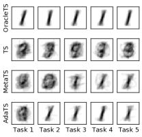
Appendix E contains more experiments. In Section E.1, we experiment with more values of $K$ and $d$, and show the robustness of $\tt AdaTS$ to missspecified meta-prior $Q$. In Section E.2, we apply $\tt AdaTS$ to bandit classification problems. In Figure 3, we show results for one of these problems, meta-learning a highly rewarding digit $1$ in the bandit setting. For each method and task $s$, we show the average digit corresponding to the pulled arms in round $1$ of task $s$. $\tt AdaTS$ learns a good meta-parameter $\mu_{*}$ almost instantly, since its average digit in task $2$ already resembles digit $1$.

6 Related Work

Two closest related works are Bastani et al. [6] and Kveton et al. [28]. Bastani et al. [6] proposed Thompson sampling that learns the prior from a sequence of pricing experiments. The algorithm is tailored to pricing and learns through forced exploration using conservative TS. Therefore, it is conservative. Bastani et al. [6] also did not derive prior-dependent bounds.

Our studied setting is identical to Kveton et al. [28]. However, the design of $\tt AdaTS$ is very different from $\tt MetaTS$. $\tt MetaTS$ samples the meta-parameter $\mu_{s}$ at the beginning of each task $s$ and uses it to compute the posterior of the task parameter $\theta_{s,*}$. Since $\mu_{s}$ is fixed within the task, $\tt MetaTS$ does not have a correct posterior of $\theta_{s,*}$ given the history. $\tt AdaTS$ marginalizes out the uncertainty in the meta-parameter $\mu_{*}$ and thus has a correct posterior of $\theta_{s,*}$ within the task. This seemingly minor difference leads to an approach that is more principled, comparably general, has a fully-Bayesian analysis beyond multi-armed bandits, and may have several-fold lower regret in practice. While it is possible that the analysis of $\tt MetaTS$ could be extended to linear bandits, the price for meta-learning would likely remain $\tilde{O}(\sqrt{m}n^{2})$. This cost arises due sampling the meta-parameter $\mu_{s}$ at the beginning of each task $s$. The price of meta-learning in our work is mere $\tilde{O}(\sqrt{mn})$, a huge improvement.

$\tt AdaTS$ is a meta-learning algorithm [39, 40, 7, 8, 17, 18]. Meta-learning has a long history in multi-armed bandits. Some of the first works are Azar et al. [5] and Gentile et al. [21], who proposed UCB algorithms for multi-task learning. Deshmukh et al. [15] studied multi-task learning in contextual bandits. Cella et al. [10] proposed a UCB algorithm that meta-learns the mean parameter vector in a linear bandit, which is akin to learning $\mu_{*}$ in Section 3.2. Another recent work is Yang et al. [43], who studied regret minimization with multiple parallel bandit instances, with the goal of learning their shared subspace. All of these works are frequentist, analyze a stronger notion of regret, and often lead to conservative algorithm designs. In contrast, we leverage the fundamentals of Bayesian reasoning to design a general-purpose algorithm that performs well when run as analyzed.

Several recent papers approached the problem of learning a bandit algorithm using policy gradients [16, 9, 27, 44, 35], including learning Thompson sampling [27, 35]. These works focus on offline optimization against a known bandit-instance distribution and have no convergence guarantees in general [9, 27]. Tuning of bandit algorithms is known to reduce regret [41, 34, 24, 23]. Typically it is ad-hoc and we believe that meta-learning is a proper way of framing this problem.

7 Conclusions

We propose $\tt AdaTS$, a fully-Bayesian algorithm for meta-learning in bandits that adapts to a sequence of bandit tasks that it interacts with. $\tt AdaTS$ attains low regret by adapting the uncertainty in both the meta and per-task parameters. We analyze the Bayes regret of $\tt AdaTS$ using information-theory tools that isolate the effect of learning the meta-parameter from that of learning the per-task parameters. For linear bandits and semi-bandits, we derive novel prior-dependent regret bounds that show that the price for learning the meta-parameter is low. Our experiments underscore the generality of $\tt AdaTS$, good out-of-the-box performance, and robustness to meta-prior misspecification.

We leave open several questions of interest. For instance, except for Section 3.4, our algorithms are for Gaussian rewards and priors, and so are their regret analyses. An extension beyond Gaussians would be of both practical and theoretical value. Our current work also relies heavily on a particular parameterization of tasks, where the mean $\theta_{s,*}$ is unknown but the covariance $\Sigma_{0}$ is known. It is not immediately obvious if a computationally-efficient extension to unknown $\Sigma_{0}$ exists.

Appendix A Algorithm Details

Our terminology is summarized below:

$\theta_{s,*}$	Bandit instance parameter in task $s$, generated as $\theta_{s,*}\sim P(\cdot;\mu_{*})$
$P(\cdot;\mu_{*})$	Task prior, a distribution over bandit instance parameter $\theta_{s,*}$
$\mu_{*}$	Meta-parameter, a parameter of the task distribution
$Q$	Meta-prior, a distribution over the meta-parameter $\mu_{*}$
$P_{s}$	Uncertainty-adjusted prior in task $s$, a distribution over $\theta_{s,*}$ conditioned on $H_{1:s-1}$
$Q_{s}$	Meta-posterior in task $s$, a distribution over $\mu_{*}$ conditioned on $H_{1:s-1}$
$Y_{s,t}$	Stochastic rewards of all arms in round $t$ of task $s$
$A_{s,t}$	Pulled arm in round $t$ of task $s$

We continue with two lemmas, which are used in the algorithmic part of the paper (Section 3).

*

Proof.

To simplify presentation, our proof is under the assumption that $\theta_{s,*}$ and $\mu_{*}$ take on countably-many values. A more general measure-theory treatment, where we would maintain measures over $\theta_{s,*}$ and $\mu_{*}$, would follow the same line of reasoning; and essentially replace all probabilities with densities. A good discussion of this topic is in Section 34 of Lattimore and Szepesvari [31].

The following convention is used in the proof. The values of random variables that we marginalize out, such as $\theta_{s,*}$ and $\mu_{*}$, are explicitly assigned. For fixed variables, such as the history $H_{1:s-1}$, we also treat $H_{1:s-1}$ as the actual value assigned to $H_{1:s-1}$.

We start with the posterior distribution of $\theta_{s,*}$ in task $s$, which can be expressed as

$$\mathbb{P}\left(\theta_{s,*}=\theta\,\middle|\,H_{1:s-1}\right) =\sum_{\mu}\mathbb{P}\left(\theta_{s,*}=\theta,\mu_{*}=\mu\,\middle|\,H_{1:s-1}\right)$$

$$=\sum_{\mu}\mathbb{P}\left(\theta_{s,*}=\theta\,\middle|\,\mu_{*}=\mu\right)\mathbb{P}\left(\mu_{*}=\mu\,\middle|\,H_{1:s-1}\right)\,.$$

The second equality holds because $\theta_{s,*}$ is independent of history $H_{1:s-1}$ given $\mu_{*}$. Now note that $\mathbb{P}\left(\mu_{*}=\mu\,\middle|\,H_{1:s-1}\right)$ is the meta-posterior in task $s$. It can be rewritten as

$$\mathbb{P}\left(\mu_{*}=\mu\,\middle|\,H_{1:s-1}\right) =\frac{\mathbb{P}\left(\mu_{*}=\mu\,\middle|\,H_{1:s-1}\right)}{\mathbb{P}\left(\mu_{*}=\mu\,\middle|\,H_{1:s-2}\right)}\mathbb{P}\left(\mu_{*}=\mu\,\middle|\,H_{1:s-2}\right)$$

$$=\frac{\mathbb{P}\left(H_{s-1}\,\middle|\,H_{1:s-2},\,\mu_{*}=\mu\right)}{\mathbb{P}\left(H_{s-1}\,\middle|\,H_{1:s-2}\right)}\mathbb{P}\left(\mu_{*}=\mu\,\middle|\,H_{1:s-2}\right)$$

$$\propto\underbrace{\mathbb{P}\left(H_{s-1}\,\middle|\,H_{1:s-2},\,\mu_{*}=\mu\right)}_{f_{1}(\mu)}\mathbb{P}\left(\mu_{*}=\mu\,\middle|\,H_{1:s-2}\right)\,,$$

where $\mathbb{P}\left(\mu_{*}=\mu\,\middle|\,H_{1:s-2}\right)$ is the meta-posterior in task $s-1$. The last step follows from the fact that $\mathbb{P}\left(H_{s-1}\,\middle|\,H_{1:s-2}\right)$ is constant in $\mu$. Now we focus on $f_{1}(\mu)$ above and rewrite it as

$$f_{1}(\mu) =\sum_{\theta}\mathbb{P}\left(H_{s-1},\,\theta_{s-1,*}=\theta\,\middle|\,H_{1:s-2},\,\mu_{*}=\mu\right)$$

$$=\sum_{\theta}\mathbb{P}\left(H_{s-1}\,\middle|\,H_{1:s-2},\,\theta_{s-1,*}=\theta,\,\mu_{*}=\mu\right)\mathbb{P}\left(\theta_{s-1,*}=\theta\,\middle|\,H_{1:s-2},\,\mu_{*}=\mu\right)$$

$$=\sum_{\theta}\underbrace{\mathbb{P}\left(H_{s-1}\,\middle|\,H_{1:s-2},\,\theta_{s-1,*}=\theta\right)}_{f_{2}(\theta)}\mathbb{P}\left(\theta_{s-1,*}=\theta\,\middle|\,\mu_{*}=\mu\right)\,.$$

In the last step, we use that the history $H_{s-1}$ is independent of $\mu_{*}$ given $H_{1:s-2}$ and $\theta_{s-1,*}$, and that the task parameter $\theta_{s-1,*}$ is independent of $H_{1:s-2}$ given $\mu_{*}$.

Now we focus on $f_{2}(\theta)$ above. To simplify notation, it is useful to define $Y_{t}=Y_{s-1,t}(A_{s-1,t})$ and $A_{t}=A_{s-1,t}$. Then we can rewrite $f_{2}(\theta)$ as

$$f_{2}(\theta) =\prod_{t=1}^{n}\mathbb{P}\left(A_{t},Y_{t}\,\middle|\,H_{1:s-1,t},\,\theta_{s-1,*}=\theta\right)$$

$$=\prod_{t=1}^{n}\mathbb{P}\left(Y_{t}\,\middle|\,A_{t},\,H_{1:s-1,t},\,\theta_{s-1,*}=\theta\right)\mathbb{P}\left(A_{t}\,\middle|\,H_{1:s-1,t},\,\theta_{s-1,*}=\theta\right)$$

$$=\prod_{t=1}^{n}\mathbb{P}\left(Y_{t}\,\middle|\,A_{t},\,\theta_{s-1,*}=\theta\right)\mathbb{P}\left(A_{t}\,\middle|\,H_{1:s-1,t}\right)\propto\mathbb{P}\left(Y_{1:n}\,\middle|\,A_{1:n},\,\theta_{s-1,*}=\theta\right)\,.$$

In the third equality, we use that the reward $Y_{t}$ is independent of history $H_{1:s-1,t}$ given the pulled arm $A_{t}$ and task parameter $\theta_{s-1,*}$, and that $A_{t}$ is independent of $\theta_{s-1,*}$ given $H_{1:s-1,t}$. In the last step, we use that $\mathbb{P}\left(A_{t}\,\middle|\,H_{1:s-1,t}\right)$ is constant in $\theta$.

Finally, we combine all above claims, note that

$$\mathbb{P}\left(\theta_{s,*}=\theta\,\middle|\,\mu_{*}=\mu\right)=\mathbb{P}\left(\theta_{s-1,*}=\theta\,\middle|\,\mu_{*}=\mu\right)=P(\theta;\mu)\,,$$

and get

$$\mathbb{P}\left(\theta_{s,*}=\theta\,\middle|\,H_{1:s-1}\right) =\sum_{\mu}P(\theta;\mu)\,\mathbb{P}\left(\mu_{*}=\mu\,\middle|\,H_{1:s-1}\right)\,,$$

$$\mathbb{P}\left(\mu_{*}=\mu\,\middle|\,H_{1:s-1}\right) =\sum_{\theta}\mathbb{P}\left(Y_{1:n}\,\middle|\,A_{1:n},\,\theta_{s-1,*}=\theta\right)P(\theta;\mu)\,\mathbb{P}\left(\mu_{*}=\mu\,\middle|\,H_{1:s-2}\right)\,.$$

These are the claims that we wanted to prove, since

$$P_{s}(\theta) =\mathbb{P}\left(\theta_{s,*}=\theta\,\middle|\,H_{1:s-1}\right)\,,$$

$$Q_{s}(\mu) =\mathbb{P}\left(\mu_{*}=\mu\,\middle|\,H_{1:s-1}\right)\,,$$

$$\mathcal{L}_{s-1}(\theta) =\mathbb{P}\left(Y_{1:n}\,\middle|\,A_{1:n},\,\theta_{s-1,*}=\theta\right)\,.$$

This concludes the proof. ∎

Lemma 1.

Fix integers $s$ and $n$, features $(x_{\ell,t})_{\ell\in[s],t\in[n]}$, and consider a generative process

$$\mu_{*} \sim\mathcal{N}(\mu_{q},\Sigma_{q})\,,$$

$$\forall\ell\in[s]:\theta_{\ell,*}\mid\mu_{*} \sim\mathcal{N}(\mu_{*},\Sigma_{0})\,,$$

$$\forall\ell\in[s],t\in[n]:Y_{\ell,t}\mid\mu_{*} \sim\mathcal{N}(x_{\ell,t}^{\top}\theta_{\ell,*},\sigma^{2})\,,$$

where all variables are drawn independently. Then $\mu_{*}\mid(Y_{\ell,t})_{\ell\in[s],\,t\in[n]}\sim\mathcal{N}(\hat{\mu},\hat{\Sigma})$ for

$$\hat{\mu} =\hat{\Sigma}\left(\Sigma_{q}^{-1}\mu_{q}+\sum_{\ell=1}^{s}\frac{B_{\ell}}{\sigma^{2}}-\frac{G_{\ell}}{\sigma^{2}}\left(\Sigma_{0}^{-1}+\frac{G_{\ell}}{\sigma^{2}}\right)^{-1}\frac{B_{\ell}}{\sigma^{2}}\right)\,,$$

$$\hat{\Sigma}^{-1} =\Sigma_{q}^{-1}+\sum_{\ell=1}^{s}\frac{G_{\ell}}{\sigma^{2}}-\frac{G_{\ell}}{\sigma^{2}}\left(\Sigma_{0}^{-1}+\frac{G_{\ell}}{\sigma^{2}}\right)^{-1}\frac{G_{\ell}}{\sigma^{2}}\,,$$

where $G_{\ell}=\sum_{t=1}^{n}x_{\ell,t}x_{\ell,t}^{\top}$ is the outer product of the features in task $\ell$ and $B_{\ell}=\sum_{t=1}^{n}x_{\ell,t}Y_{\ell,t}$ is their sum weighted by observations.

Proof.

The claim is proved in Appendix D of Kveton et al. [28]. We restate it for completeness. ∎

Appendix B Proofs for Section 4.1: Generic Regret Bound

B.1 Preliminaries and Omitted Definitions

Notation for History:

Let us recall that $H_{s,t}=((A_{s,1},Y_{s,1}),\dots,(A_{s,t-1},Y_{s,t-1}))$ denote the events in task $s$ upto and excluding round $t$ for all $t\geq 1$ ($H_{s,1}=\emptyset$). The events in task $s$ is denoted as $H_{s}=H_{s,n+1}$ and all the events upto and including stage $s$ is denoted as $H_{1:s}=\cup_{s^{\prime}=1}^{s}H_{s^{\prime}}$. Let us also define history upto and excluding round $t$ in task $s$ as $H_{1:s,t}=\{H_{1:s-1}\cup H_{s,t}\}$, with $H_{1:s}=H_{1:s,n+1}$. Given the history upto and excluding round $t$ in task $s$, the conditional probability is given as $\mathbb{P}_{s,t}(\cdot)=\mathbb{P}[\cdot\mid H_{1:s,t}]$, and the conditional expectation is given as $\mathbb{E}_{s,t}(\cdot)=\mathbb{E}[\cdot\mid H_{1:s,t}]$. Note $\mathbb{P}[\cdot]$ and $\mathbb{E}[\cdot]$ denote the unconditional probability and expectation, respectively.

History dependent Entropy and Mutual Information:

We now define the entropy and mutual information terms as a function of history.

The mutual information between the parameter $\theta_{s,*}$, and the action ($A_{s,t}$) and reward ($Y_{s,t}$) at the beginning of round $t$ in task $s$, for any $s\leq m$ and $t\leq n$, as a function of history is defined as

$$I_{s,t}(\theta_{s,*};A_{s,t},Y_{s,t})=\mathbb{E}_{s,t}\left[\log\left(\frac{\mathbb{P}_{s,t}(\theta_{s,*},Y_{s,t},A_{s,t})}{\mathbb{P}_{s,t}(\theta_{s,*})\mathbb{P}_{s,t}(Y_{s,t},A_{s,t})}\right)\right]$$

We also define the mutual information between the parameter $\mu_{*}$, and the action ($A_{s,t}$) and reward ($Y_{s,t}$) at the beginning of round $t$ in task $s$, for any $s\leq m$ and $t\leq n$ as

$$I_{s,t}(\mu_{*};A_{s,t},Y_{s,t})=\mathbb{E}_{s,t}\left[\log\left(\frac{\mathbb{P}_{s,t}(\mu_{*},Y_{s,t},A_{s,t})}{\mathbb{P}_{s,t}(\mu_{*})\mathbb{P}_{s,t}(Y_{s,t},A_{s,t})}\right)\right]$$

Further, the history dependent conditional mutual information between $(\mu_{*},\theta_{s,*})$, and $A_{s,t}$ and $Y_{s,t}$, namely $I_{s,t}(\theta_{s,*},\mu_{*};A_{s,t},Y_{s,t})$, is defined below.

$$I_{s,t}(\theta_{s,*},\mu_{*};A_{s,t},Y_{s,t})=\mathbb{E}_{s,t}\left[\log\left(\frac{\mathbb{P}_{s,t}(\theta_{s,*},\mu_{*},Y_{s,t},A_{s,t})}{\mathbb{P}_{s,t}(\theta_{s,*},\mu_{*})\mathbb{P}_{s,t}(Y_{s,t},A_{s,t})}\right)\right]$$

Finally, we define the history dependent conditional mutual information between $\theta_{s,*}$, and $A_{s,t}$ and $Y_{s,t}$ given $\mu_{*}$ as $I_{s,t}(\theta_{s,*};A_{s,t},Y_{s,t}\mid\mu_{*})$.

$$I_{s,t}(\theta_{s,*};A_{s,t},Y_{s,t}\mid\mu_{*})=\mathbb{E}_{s,t}\left[\log\left(\frac{\mathbb{P}_{s,t}(\theta_{s,*},Y_{s,t},A_{s,t}\mid\mu_{*})}{\mathbb{P}_{s,t}(\theta_{s,*}\mid\mu_{*})\mathbb{P}_{s,t}(Y_{s,t},A_{s,t}\mid\mu_{*})}\right)\right]$$

The conditional entropy terms are defined as follows:

$$h_{s,t}(\theta_{s,*}) =\mathbb{E}_{s,t}\left[-\log\left(\mathbb{P}_{s,t}(\theta_{s,*})\right)\right]\,,$$

$$\quad h_{s,t}(\mu_{*}) =\mathbb{E}_{s,t}\left[-\log\left(\mathbb{P}_{s,t}(\mu_{*})\right)\right]\,,$$

$$h_{s,t}(\theta_{s,*}\mid\mu_{*}) =\mathbb{E}_{s,t}\left[-\log\left(\mathbb{P}_{s,t}(\theta_{s,*}\mid\mu_{*})\right)\right]\,.$$

Therefore, all the different mutual information terms $I_{s,t}(\cdot;A_{s,t},Y_{s,t})$, and the entropy terms $h_{s,t}(\cdot)$ are random variables that depends on the history $H_{1:s,t}$.

We next state some entropy and mutual information relationships which we will use later.

Proposition 2.

For all $s$, $t$, and any history $H_{1:s,t}$, the following hold

$$I_{s,t}(\theta_{s,*},\mu_{*};A_{s,t},Y_{s,t}) =I_{s,t}(\mu_{*};A_{s,t},Y_{s,t})+I_{s,t}(\theta_{s,*};A_{s,t},Y_{s,t}\mid\mu_{*})\,,$$

$$I_{s,t}(\theta_{s,*};A_{s,t},Y_{s,t}) =h_{s,t}(\theta_{s,*})-h_{s,t+1}(\theta_{s,*})\,.$$

History Independent Entropy and Mutual Information:

The history independent conditional mutual information and entropy terms are then given by taking expectation over the possible histories

$$I(\cdot;A_{s,t},Y_{s,t}\mid H_{1:s,t})=\mathbb{E}[I_{s,t}(\cdot;A_{s,t},Y_{s,t})],\quad h(\cdot\mid H_{1:s,t})=\mathbb{E}[h_{s,t}(\cdot)]$$

$$I(\cdot;A_{s,t},Y_{s,t}\mid\mu_{*},H_{1:s,t})=\mathbb{E}[I_{s,t}(\cdot;A_{s,t},Y_{s,t}\mid\mu_{*})],\quad h(\cdot\mid\mu_{*},H_{1:s,t})=\mathbb{E}[h_{s,t}(\cdot\mid\mu_{*})]$$

An important quantity that will play a pivotal role in our regret decomposition is the conditional mutual information of the meta-parameter given the entire history, which is expressed as

$$I(\mu_{*};H_{1:m})=\sum_{s=1}^{m}\sum_{t=1}^{n}I(\mu_{*};A_{s,t},Y_{s,t}\mid H_{1:s,t})=\mathbb{E}\sum_{s=1}^{m}\sum_{t=1}^{n}I_{s,t}(\mu_{*};A_{s,t},Y_{s,t}).$$

The first equality is due to chain rule of mutual information, where at each round the new history $H_{1:s,t+1}=H_{1:s,t}\cup(A_{s,t},Y_{s,t})$.

Similarly, in each stage $s$, the mutual information between parameter $\theta_{s,*}$ and the events in stage $s$, i.e. $H_{s}$, conditioned on $\mu_{*}$ and history up to task $(s-1)$ is key in quantifying the local regret of task $s$. Which is again expressed as

$$I(\theta_{s,*};H_{s}\mid\mu_{*},H_{1:s-1})=\sum_{t=1}^{n}I(\theta_{s,*};A_{s,t},Y_{s,t}\mid\mu_{*},H_{1:s,t})=\mathbb{E}\sum_{t=1}^{n}I_{s,t}(\theta_{s,*};A_{s,t},Y_{s,t}\mid\mu_{*}).$$

The first inequality again follows chain rule of mutual information with new history being the combination of old history, and the action and the observed reward in the current round.

We further have the relation of mutual information and conditional entropy as

$$I(\theta_{s,*};H_{s}\mid\mu_{*},H_{1:s-1}) =h(\theta_{s,*}\mid\mu_{*},H_{1:s-1})-h(\theta_{s,*}\mid\mu_{*},H_{1:s})\,,$$

$$I(\mu_{*};H_{1:m}) =h(\mu_{*})-h(\mu_{*}\mid H_{1:m})\,.$$

Weyl’s Inequalities:

In this paper, the matrices under consideration are all Positive Semi-definite (PSD) and symmetric. Thus, the eignevalues are non-negative and admits a total order. We denote the eigenvalues of a PSD matrix $A\in\mathbb{R}^{d}$, for any integer $d\geq 1$, as $\lambda_{d}(A)\leq\dots\leq\lambda_{1}(A)$; where $\lambda_{1}(A)$ is the maximum eigenvalue, and $\lambda_{d}(A)$ is the minimum eigenvalue of the PSD matrix $A$.

Weyl’s inequality states for two Hermitian matrices (PSD and Symmetric in reals) $A$ and $B$,

$$\lambda_{j}(A)+\lambda_{k}(B)\leq\lambda_{i}(A+B)\leq\lambda_{r}(A)+\lambda_{s}(B),\quad\forall\,j+k-d\geq i\geq r+s-1.$$

The two important relations, derived from Weyl’s inequality, that we frequently use in the proofs are given next. For PSD and symmetric matrices $\{A_{i}\}$ we have

$$\lambda_{1}(\sum_{i}A_{i})\leq\sum_{i}\lambda_{1}(A_{i}),\quad\text{ and }\lambda_{d}(\sum_{i}A_{i})\geq\sum_{i}\lambda_{d}(A_{i}).$$

*

Proof.

The proof follows through the series of inequalities below (explanation added).

$$R(m,n) =\mathbb{E}\sum_{s,t}[\Delta_{s,t}]$$

$$[\text{Eq.}~{}\eqref{a:info}] \leq\mathbb{E}\sum_{s,t}\Gamma_{s,t}\sqrt{I_{s,t}(\theta_{s,*};A_{s,t},Y_{s,t})}+\mathbb{E}\sum_{s,t}\epsilon_{s,t}$$

$$[I(X;Z)\leq I(X,Y;Z)] \leq\mathbb{E}\sum_{s,t}\Gamma_{s,t}\sqrt{I_{s,t}(\theta_{s,*},\mu_{*};A_{s,t},Y_{s,t})}+\mathbb{E}\sum_{s,t}\epsilon_{s,t}$$

$$[\text{Chain Rule}] =\mathbb{E}\sum_{s,t}\Gamma_{s,t}\sqrt{I_{s,t}(\mu_{*};A_{s,t},Y_{s,t})+I_{s,t}(\theta_{s,*};A_{s,t},Y_{s,t}\mid\mu_{*})}+\mathbb{E}\sum_{s,t}\epsilon_{s,t}$$

$$[\sqrt{a+b}\mathtt{\leq}\sqrt{a}\mathtt{+}\sqrt{b}] \leq\mathbb{E}\sum_{s,t}\Gamma_{s,t}\sqrt{I_{s,t}(\mu_{*};A_{s,t},Y_{s,t})}+\mathbb{E}\sum_{s,t}\Gamma_{s,t}\sqrt{I_{s,t}(\theta_{s,*};A_{s,t},Y_{s,t}\mid\mu_{*})}$$

$$+\mathbb{E}\sum_{s,t}\epsilon_{s,t}$$

$$[\Gamma_{s,t}\leq\Gamma_{s}\leq\Gamma,\forall s,t,\text{ w.p. }1] \leq\Gamma\,\mathbb{E}\sum_{s,t}\sqrt{I_{s,t}(\mu_{*};A_{s,t},Y_{s,t})}+\sum_{s}\Gamma_{s}\left[\mathbb{E}\sum_{t}\sqrt{I_{s,t}(\theta_{s,*};A_{s,t},Y_{s,t}\mid\mu_{*})}\right]$$

$$+\mathbb{E}\sum_{s,t}\epsilon_{s,t}$$

$$[\text{Jensen's Inequality}] \leq\Gamma\sum_{s,t}\sqrt{\mathbb{E}I_{s,t}(\mu_{*};A_{s,t},Y_{s,t})}+\sum_{s}\Gamma_{s}\sum_{t}\sqrt{\mathbb{E}I_{s,t}(\theta_{s,*};A_{s,t},Y_{s,t}\mid\mu_{*})}$$

$$+\mathbb{E}\sum_{s,t}\epsilon_{s,t}$$

$$[\text{Cauchy-Schwarz}] \leq\Gamma\sqrt{mn\sum_{s,t}\mathbb{E}I_{s,t}(\mu_{*};A_{s,t},Y_{s,t})}+\sum_{s}\Gamma_{s}\sqrt{n\sum_{t}\mathbb{E}I_{s,t}(\theta_{s,*};A_{s,t},Y_{s,t}\mid\mu_{*})}$$

$$+\mathbb{E}\sum_{s,t}\epsilon_{s,t}$$

$$[\text{Chain Rule}] =\Gamma\sqrt{mnI(\mu_{*};H_{1:m})}+\sum_{s}\Gamma_{s}\sqrt{nI(\theta_{s,*};H_{s}\mid\mu_{*},H_{1:s-1})}+\mathbb{E}\sum_{s,t}\epsilon_{s,t}$$

• The first inequality follows due to Eq. (3).

• The second inequality uses the fact that $I(X;Z)\leq I(X,Y;Z)$ for any random variables $X$, $Y$, and $Z$. Here $X=\theta_{s,*}$, $Y=\mu_{*}$, and $Z=(A_{s,t},Y_{s,t})$.

• The second equality uses the chain rule $I(X,Y;Z)=I(X;Z)+I(X;Z\mid Y)$, as stated in Proposition 2, with the same random variables $X$, $Y$, and $Z$.

• The Jensen’s inequality uses concavity of $\sqrt{\cdot}$.

∎

Appendix C Proofs for Section 4.2: Linear Bandit

C.1 Marginalization of the Variables

Notation in Marginalization:

Let $\mathcal{N}(x;\mu,\Sigma)$ denote a (possibly multivariate) Gaussian p.d.f. with mean $\mu$ and covariance matrix $\Sigma$ for variable $x$. We now recall the notations of posterior distributions at different time of our algorithm

$$P(\theta;\mu)=\mathbb{P}\left(\theta_{s,*}=\theta\,\middle|\,\mu_{*}=\mu\right)=\mathcal{N}(\theta;\mu,\Sigma_{0}),\quad Q(\mu)=\mathbb{P}\left(\mu_{*}=\mu\right)=\mathcal{N}(\mu;\mu_{0},\Sigma_{q})$$

$$P_{s}(\theta)=\mathbb{P}\left(\theta_{s,*}=\theta\,\middle|\,H_{1:s-1}\right)=\int_{\mu}P(\theta;\mu)Q_{s}(\mu)\mathop{}\!\mathrm{d}\mu,$$

$$P_{s,t}(\theta)=\mathbb{P}\left(\theta_{s,*}=\theta\,\middle|\,H_{1:s,t}\right)\propto\mathbb{P}\left(H_{s,t}\,\middle|\,\theta_{s,*}=\theta\right)P_{s}(\theta),$$

$$Q_{s}(\mu) =\mathbb{P}\left(\mu_{*}=\mu\,\middle|\,H_{1:s-1}\right)=\int_{\theta}\mathbb{P}\left(H_{s-1}\,\middle|\,\theta_{s-1,*}=\theta\right)P(\theta;\mu)\mathop{}\!\mathrm{d}\theta Q_{s-1}(\mu)$$

The marginalization is proved in an inductive manner due to the dependence of the action matrix $A$ on the history. We recall the expression of the rewards,

$$Y_{s,t}=A_{s,t}^{T}\theta_{s,*}+w_{s,t}$$

In each round $t$ and task $s$, given the parameter $\theta_{s,*}$ and the action $A_{s,t}$, the reward $Y_{s,t}$ has the p.d.f. $\mathbb{P}(Y_{s,t}\mid\theta_{s,*},A_{s,t})=\mathcal{N}(Y_{s,t};A_{s,t}^{T}\theta_{s,*},\sigma^{2})$. Let $\propto_{X}$ denote that the proportionality constant is independent of $X$ (possibly a set).

We obtain the posterior probability of the true parameter in task $s$ in round $t$, given the true parameter $\mu_{*}$. Let us define for all $s\leq m$, and $t\leq n$.

$$P_{s,t,\mu_{*}}(\theta)=\mathbb{P}(\theta_{s,*}=\theta\mid\mu_{*},H_{1:s,t})\propto\prod_{t^{\prime}=1}^{t-1}\mathbb{P}(Y_{s,t^{\prime}}\mid\theta_{s,*}=\theta,A_{s,t^{\prime}})P(\theta,\mu_{*})$$

$$\propto_{\theta}\prod_{t^{\prime}=1}^{t-1}\exp\left(-\frac{(Y_{s,t^{\prime}}-A_{s,t^{\prime}}^{T}\theta)^{2}}{2\sigma^{2}}\right)\mathcal{N}(\theta;\mu_{*},\Sigma_{0})$$

$$\propto_{\theta}\exp\left(-\sum_{t^{\prime}=1}^{t-1}(\theta-A_{s,t^{\prime}}Y_{s,t^{\prime}})^{T}\tfrac{A_{s,t^{\prime}}A^{T}_{s,t^{\prime}}}{2\sigma^{2}}(\theta-A_{s,t^{\prime}}Y_{s,t^{\prime}})\right)\mathcal{N}(\theta;\mu_{*},\Sigma_{0})$$

$$\propto_{\theta}\exp\left(-\left(\theta-\bar{\theta}\right)^{T}\sum_{t^{\prime}=1}^{t-1}\tfrac{A_{s,t^{\prime}}A^{T}_{s,t^{\prime}}}{2\sigma^{2}}\left(\theta-\bar{\theta}\right)\right)\mathcal{N}(\theta;\mu_{*},\Sigma_{0})\quad\left[\bar{\theta}=(\sum_{t^{\prime}=1}^{t-1}\tfrac{A_{s,t^{\prime}}A^{T}_{s,t^{\prime}}}{\sigma^{2}})^{-1}\sum_{t^{\prime}=1}^{t-1}A_{s,t^{\prime}}Y_{s,t^{\prime}}\right]$$

$$\propto_{\theta}\mathcal{N}\left(\theta;\hat{\Sigma}_{s,t,\mu_{*}}\left(\Sigma_{0}^{-1}\mu_{*}+\sum_{t^{\prime}=1}^{t-1}A_{s,t^{\prime}}Y_{s,t^{\prime}}\right),\hat{\Sigma}_{s,t,\mu_{*}}\right)\quad\left[\hat{\Sigma}_{s,t,\mu_{*}}^{-1}=\Sigma_{0}^{-1}+\sum_{t^{\prime}=1}^{t-1}\tfrac{A_{s,t^{\prime}}A^{T}_{s,t^{\prime}}}{\sigma^{2}}\right]$$

We now obtain the posterior probability of the true parameter in task $s$ in round $t$ as by taking integral over the prior of the parameter $\mu_{*}$.

$$P_{s,t}(\theta)=\mathbb{P}(\theta_{s,*}=\theta\mid H_{1:s,t})\propto\prod_{t^{\prime}=1}^{t-1}\mathbb{P}(Y_{s,t^{\prime}}\mid\theta_{s,*}=\theta,A_{s,t^{\prime}})\int_{\mu}P(\theta,\mu)Q_{s}(\mu)d\mu$$

$$\propto_{\theta}\prod_{t^{\prime}=1}^{t-1}\exp\left(-\frac{(Y_{s,t^{\prime}}-A_{s,t^{\prime}}^{T}\theta)^{2}}{2\sigma^{2}}\right)\int_{\mu}\mathcal{N}(\theta;\mu,\Sigma_{0})\mathcal{N}(\mu;\hat{\mu}_{s},\hat{\Sigma}_{s})d\mu$$

$$\propto_{\theta}\exp\left(-\sum_{t^{\prime}=1}^{t-1}(\theta-A_{s,t^{\prime}}Y_{s,t^{\prime}})^{T}\tfrac{A_{s,t^{\prime}}A^{T}_{s,t^{\prime}}}{2\sigma^{2}}(\theta-A_{s,t^{\prime}}Y_{s,t^{\prime}})\right)\mathcal{N}(\theta;\hat{\mu}_{s},\Sigma_{0}+\hat{\Sigma}_{s})$$

$$\propto_{\theta}\exp\left(-\sum_{t^{\prime}=1}^{t-1}(\theta-A_{s,t^{\prime}}Y_{s,t^{\prime}})^{T}\tfrac{A_{s,t^{\prime}}A^{T}_{s,t^{\prime}}}{2\sigma^{2}}(\theta-A_{s,t^{\prime}}Y_{s,t^{\prime}})\right)\mathcal{N}(\theta;\hat{\mu}_{s},\Sigma_{0}+\hat{\Sigma}_{s})$$

$$\propto_{\theta}\exp\left(-\left(\theta-\bar{\theta}\right)^{T}\sum_{t^{\prime}=1}^{t-1}\tfrac{A_{s,t^{\prime}}A^{T}_{s,t^{\prime}}}{2\sigma^{2}}\left(\theta-\bar{\theta}\right)\right)\mathcal{N}(\theta;\hat{\mu}_{s},\Sigma_{0}+\hat{\Sigma}_{s})\quad\left[\bar{\theta}=(\sum_{t^{\prime}=1}^{t-1}\tfrac{A_{s,t^{\prime}}A^{T}_{s,t^{\prime}}}{\sigma^{2}})^{-1}\sum_{t^{\prime}=1}^{t-1}A_{s,t^{\prime}}Y_{s,t^{\prime}}\right]$$

$$\propto_{\theta}\mathcal{N}\left(\theta;(\sum_{t^{\prime}=1}^{t-1}\tfrac{A_{s,t^{\prime}}A^{T}_{s,t^{\prime}}}{\sigma^{2}})^{-1}\sum_{t^{\prime}=1}^{t-1}A_{s,t^{\prime}}Y_{s,t^{\prime}},(\sum_{t^{\prime}=1}^{t-1}\tfrac{A_{s,t^{\prime}}A^{T}_{s,t^{\prime}}}{\sigma^{2}})^{-1}\right)\mathcal{N}(\theta;\hat{\mu}_{s},\Sigma_{0}+\hat{\Sigma}_{s})$$

$$\propto_{\theta}\mathcal{N}\left(\theta;\hat{\Sigma}_{s,t}\left((\Sigma_{0}+\hat{\Sigma}_{s})^{-1}\hat{\mu}_{s}+\sum_{t^{\prime}=1}^{t-1}A_{s,t^{\prime}}Y_{s,t^{\prime}}\right),\hat{\Sigma}_{s,t}\right)\quad\left[\hat{\Sigma}_{s,t}^{-1}=(\Sigma_{0}+\hat{\Sigma}_{s})^{-1}+\sum_{t^{\prime}=1}^{t-1}\tfrac{A_{s,t^{\prime}}A^{T}_{s,t^{\prime}}}{\sigma^{2}}\right]$$

Thus, for $\hat{\mu}_{s,t}=\hat{\Sigma}_{s,t}\left((\Sigma_{0}+\hat{\Sigma}_{s})^{-1}\hat{\mu}_{s}+\sum_{t^{\prime}=1}^{t-1}A_{s,t^{\prime}}Y_{s,t^{\prime}}\right)$, the parameter conditioned on the history is distributed as $\theta_{s,*}\mid H_{1:s,t}\sim\mathcal{N}(\hat{\mu}_{s,t},\hat{\Sigma}_{s,t})$.

We now compute the posterior of the meta-parameter $\mu_{*}$ in a similar way, but some of the computation can be avoided by using Lemma 1.

$$Q_{s+1}(\mu) =\int_{\theta}\mathbb{P}(H_{s}\mid\theta_{s,*}=\theta)P(\theta;\mu)d\theta Q_{s}(\mu)$$

$$\propto_{\theta,\mu}\int_{\theta}\prod_{t=1}^{n}\mathbb{P}(Y_{s,t}\mid\theta_{s,*}=\theta,A_{s,t})P(\theta,\mu)d\theta Q_{s}(\mu)$$

$$\propto_{\theta,\mu}\prod_{\ell=1}^{s}\int_{\theta_{\ell}}\prod_{t=1}^{n}\mathbb{P}(Y_{\ell,t}\mid\theta_{\ell,*}=\theta_{\ell},A_{\ell,t})P(\theta_{\ell},\mu)d\theta_{s}Q_{0}(\mu)$$

$$=\mathcal{N}(\hat{\mu}_{s+1},\hat{\Sigma}_{s+1})$$

The second equality is obtained by expanding out the $Q_{s}(\mu)$ expressions iteratively, and using the fact that $Q_{0}(\mu)$ is the prior distribution of $\mu$ at the beginning. The final equality follows from the application of Lemma 1, by observing that the expression describes a setting identical to the setting therein, with actions $x_{\ell,t}=A_{\ell,t}$ for all $\ell\in[s]$ and $t\in[n]$. The probability of playing the actions $A_{\ell,t}$ (as oppossed to fixed $x_{\ell,t}$ in Lemma 1) are absorbed by the proportionality constant.

Recall that we have due to Lemma 1, for $G_{\ell}=\sum_{t=1}^{n}A_{\ell,t}A^{T}_{\ell,t},\,\forall\ell\in[m]$ and for any $s\in[m]$,

$$\hat{\Sigma}_{s}^{-1}=\Sigma_{q}^{-1}+\sum_{\ell=1}^{s-1}\tfrac{G_{\ell}}{\sigma^{2}}-\tfrac{G_{\ell}}{\sigma^{2}}\left(\Sigma_{0}^{-1}+\tfrac{G_{\ell}}{\sigma^{2}}\right)^{-1}\tfrac{G_{\ell}}{\sigma^{2}}=\Sigma_{q}^{-1}+\sum_{\ell=1}^{s-1}\tfrac{G_{\ell}}{\sigma^{2}}\left(\Sigma_{0}^{-1}+\tfrac{G_{\ell}}{\sigma^{2}}\right)^{-1}\Sigma_{0}^{-1}.$$

Further, if in task $\ell$ if forced exploration is used, then $G_{\ell}$ is invertible, and using Woodbury matrix identity we have

$$\tfrac{G_{\ell}}{\sigma^{2}}\left(\Sigma_{0}^{-1}+\tfrac{G_{\ell}}{\sigma^{2}}\right)^{-1}\Sigma_{0}^{-1}=\left(\Sigma_{0}+(\tfrac{G_{\ell}}{\sigma^{2}})^{-1}\right)^{-1}.$$

C.2 Proof of Lemma 2

*

Proof.

We obtain the conditional mutual entropy of $\theta_{s,*}$ given the history upto $(s-1)$-th task and $\theta$ (similar to Lu et al.[33])

$$I(\theta_{s,*};H_{s}\mid\mu_{*},H_{1:s-1}) =h(\theta_{s,*}\mid\mu_{*},H_{1:s-1})-h(\theta_{s,*}\mid\mu_{*},H_{1:s})$$

$$=\mathbb{E}[h_{s-1,n+1}(\theta_{s,*}\mid\mu_{*})]-\mathbb{E}[h_{s,n+1}(\theta_{s,*}\mid\mu_{*})]$$

$$=\tfrac{1}{2}\log(\operatorname{det}(2\pi e\Sigma_{0}))-\mathbb{E}[\tfrac{1}{2}\log(\operatorname{det}(2\pi e\hat{\Sigma}_{s,n,\mu_{*}}))]$$

$$=\tfrac{1}{2}\mathbb{E}[\log(\operatorname{det}(\Sigma_{0})\operatorname{det}(\hat{\Sigma}_{s,n,\mu_{*}}^{-1}))]$$

$$=\tfrac{1}{2}\mathbb{E}\left[\prod_{i=1}^{d}\lambda_{i}(\Sigma_{0})\lambda_{i}(\hat{\Sigma}_{s,n,\mu_{*}}^{-1})))\right]$$

$$\leq\tfrac{1}{2}\log\left(\prod_{i=1}^{d}\lambda_{i}(\Sigma_{0})\left(\frac{1}{\lambda_{i}(\Sigma_{0})}+\frac{n}{\sigma^{2}}\right)\right)$$

$$\leq\tfrac{d}{2}\log\left(1+n\frac{\lambda_{1}(\Sigma_{0})}{\sigma^{2}}\right)$$

The first inequality follows from the definition of conditional mutual information (here we have outer expectation). Using the relation between the history-independent and history-dependent entropy terms we obtain the second inequality. Note that $h_{s-1,n+1}(\theta_{s,*}\mid\mu_{*})$ is independent of history, as the $\theta_{s,*}$ given $\mu_{*}$ does not depend on old tasks.

For the first inequality, we derive the following history independent bound.

$$\lambda_{i}(\hat{\Sigma}_{s,n,\mu_{*}}^{-1}) =\lambda_{i}\left(\Sigma_{0}^{-1}+\tfrac{1}{\sigma^{2}}\sum_{t^{\prime}=1}^{n}A_{s,t^{\prime}}A_{s,t^{\prime}}^{T}\right)$$

$$\leq\lambda_{i}\left(\Sigma_{0}^{-1}\right)+\lambda_{1}\left(\sum_{t^{\prime}=1}^{n}\frac{A_{s,t^{\prime}}A_{s,t^{\prime}}^{T}}{\sigma^{2}}\right)$$

$$\leq\frac{1}{\lambda_{i}(\Sigma_{0})}+tr\left(\sum_{t^{\prime}=1}^{n}\frac{A_{s,t^{\prime}}A_{s,t^{\prime}}^{T}}{\sigma^{2}}\right)$$

$$\leq\frac{1}{\lambda_{i}(\Sigma_{0})}+\frac{n}{\sigma^{2}}$$

The matrices $\tfrac{1}{\sigma^{2}}\sum_{t^{\prime}=1}^{n}A_{s,t^{\prime}}A_{s,t^{\prime}}^{T}$, and $\Sigma_{0}^{-1}$ are Hermitian matrices, giving us the first inequality by applicaiton of Weyl’s inequality. The last inequality first uses linearity of trace, and $tr(A_{s,t^{\prime}}A_{s,t^{\prime}}^{T})=tr(A_{s,t^{\prime}}^{T}A_{s,t^{\prime}})\leq 1$, by Assumption 1.

Similarly, we derive the mutual information of the meta-parameter of $\theta$ given the history as follows

$$I(\mu_{*};H_{1:m}) =h(\mu_{*})-h(\mu_{*}\mid H_{1:m})$$

$$=h(\mu_{*})-\mathbb{E}[h_{m,n+1}(\mu_{*})]$$

$$=\tfrac{1}{2}\log(\operatorname{det}(2\pi e\Sigma_{q}))-\mathbb{E}[\tfrac{1}{2}\log(\operatorname{det}(2\pi e\hat{\Sigma}_{m+1}))]$$

$$=\tfrac{1}{2}\mathbb{E}[\log(\operatorname{det}(\Sigma_{q})\operatorname{det}(\hat{\Sigma}_{m+1}^{-1}))]$$

$$\leq\tfrac{d}{2}\log\left(1+\frac{mn\lambda_{1}(\Sigma_{q})}{n\lambda_{d}(\Sigma_{0})+\sigma^{2}}\right)$$

For the final inequality above, we derive a history independent bounds in a similar manner.

$$\lambda_{i}(\hat{\Sigma}^{-1}_{m+1})\leq\lambda_{i}(\Sigma_{q}^{-1})+\lambda_{1}\left(\sum_{s^{\prime}=1}^{m}\left(\Sigma_{0}+(\sum_{t^{\prime}=1}^{n}\tfrac{A_{s^{\prime},t^{\prime}}A^{T}_{s^{\prime},t^{\prime}}}{\sigma^{2}})^{-1}\right)^{-1}\right)$$

$$\leq\lambda_{i}(\Sigma_{q}^{-1})+\sum_{s^{\prime}=1}^{m}\lambda_{1}\left(\left(\Sigma_{0}+(\sum_{t^{\prime}=1}^{n}\tfrac{A_{s^{\prime},t^{\prime}}A^{T}_{s^{\prime},t^{\prime}}}{\sigma^{2}})^{-1}\right)^{-1}\right)$$

$$\leq\frac{1}{\lambda_{i}(\Sigma_{q})}+\sum_{s^{\prime}=1}^{m}\lambda_{d}^{-1}\left(\Sigma_{0}+(\sum_{t^{\prime}=1}^{n}\tfrac{A_{s^{\prime},t^{\prime}}A^{T}_{s^{\prime},t^{\prime}}}{\sigma^{2}})^{-1}\right)$$

$$\leq\frac{1}{\lambda_{i}(\Sigma_{q})}+\sum_{s^{\prime}=1}^{m}\left(\lambda_{d}(\Sigma_{0})+\lambda_{d}\left((\sum_{t^{\prime}=1}^{n}\tfrac{A_{s^{\prime},t^{\prime}}A^{T}_{s^{\prime},t^{\prime}}}{\sigma^{2}})^{-1}\right)\right)^{-1}$$

$$\leq\frac{1}{\lambda_{i}(\Sigma_{q})}+\sum_{s^{\prime}=1}^{m}\left(\lambda_{d}(\Sigma_{0})+\lambda_{1}^{-1}(\sum_{t^{\prime}=1}^{n}\tfrac{A_{s^{\prime},t^{\prime}}A^{T}_{s^{\prime},t^{\prime}}}{\sigma^{2}})\right)^{-1}$$

$$\leq\frac{1}{\lambda_{i}(\Sigma_{q})}+\sum_{s^{\prime}=1}^{m}\left(\lambda_{d}(\Sigma_{0})+\tfrac{\sigma^{2}}{n}\right)^{-1}=\frac{1}{\lambda_{i}(\Sigma_{q})}+\frac{mn}{n\lambda_{d}(\Sigma_{0})+\sigma^{2}}$$

∎

C.3 Proof of Lemma 2

*

Proof.

We next derive the confidence interval bounds, similar to Lu et al. [33], for the reward $Y_{s,t}$ around it’s mean conditioned on the history $H_{s-1}\cup H_{s,t-1}$. Let $\hat{\theta}_{s,t}$ be the parameter sampled by TS in task $s$ and round $t$, when we do not have forced exploration.

$$\mathbb{E}_{s,t}[\Delta_{s,t}] =\mathbb{E}_{s,t}[A_{s,*}^{T}\theta_{s,*}-A_{s,t}^{T}\theta_{s,*}]=\mathbb{E}_{s,t}[A_{s,t}^{T}\hat{\theta}_{s,t}-A_{s,t}^{T}\theta_{s,*}]$$

The last equality holds as for Thompson sampling ($\stackrel{{\scriptstyle d}}{{=}}$ denotes equal distribution)

$$A_{s,*}^{T}\theta_{s,*}\mid H_{1:s,t}\stackrel{{\scriptstyle d}}{{=}}A_{s,t}^{T}\hat{\theta}_{s,t}\mid H_{1:s,t}.$$

When for task $s$ and round $t$ we have forced exploration the bound is given as

$$\mathbb{E}_{s,t}[\Delta_{s,t}] =\mathbb{E}_{s,t}[A_{s,t}^{T}\hat{\theta}_{s,t}-A_{s,t}^{T}\theta_{s,*}]+\mathbb{E}_{s,t}[A_{s,*}^{T}\theta_{s,*}-A_{s,t}^{T}\hat{\theta}_{s,t}]$$

$$\leq\mathbb{E}_{s,t}[A_{s,t}^{T}\hat{\theta}_{s,t}-A_{s,t}^{T}\theta_{s,*}]+2\mathbb{E}_{s,t}[\max_{a\in\mathcal{A}}|a^{T}\theta_{s,*}|]$$

$$\leq\mathbb{E}_{s,t}[A_{s,t}^{T}\hat{\theta}_{s,t}-A_{s,t}^{T}\theta_{s,*}]+2\mathbb{E}_{s,t}[\|\theta_{s,*}\|_{2}].$$

In the second last inequality we use the fact that $\theta_{s,*}\mid H_{1:s,t}\stackrel{{\scriptstyle d}}{{=}}\hat{\theta}_{s,t}\mid H_{1:s,t}$.

Recall $Y_{s,t}(a)$ denote the reward obtained by taking action $a$ in task $s$ and round $t$. Also recall that $\hat{\theta}_{s,t}\mid H_{1:s,t}\sim\mathcal{N}(\hat{\mu}_{s,t},\hat{\Sigma}_{s,t})$. Let us consider the set

$$\Theta_{s,t}=\{\theta:\mid a^{T}\theta-a^{T}\hat{\theta}_{s,t}\mid\leq\tfrac{\Gamma_{s,t}}{2}\sqrt{I_{s,t}(\theta_{s,*};a,Y_{s,t}(a))},\forall a\in\mathcal{A}\}.$$

The history dependent conditional mutual entropy of $\theta_{s,*}$ given the history $H_{s-1}\cup H_{s,t}$ (not $\mu_{*}$) (which will be useful in deriving concentration bounds) as

$$I_{s,t}(\theta_{s,*};A_{s,t},Y_{s,t}) =h_{s,t}(\theta_{s,*})-h_{s,t+1}(\theta_{s,*})$$

$$=\tfrac{1}{2}\log(\operatorname{det}(2\pi e(\hat{\Sigma}_{s,t-1})))-\tfrac{1}{2}\log(\operatorname{det}(2\pi e\hat{\Sigma}_{s,t}))$$

$$=\tfrac{1}{2}\log(\operatorname{det}(\hat{\Sigma}_{s,t-1}\hat{\Sigma}^{-1}_{s,t}))$$

$$=\tfrac{1}{2}\log\left(\operatorname{det}\left(I+\hat{\Sigma}_{s,t-1}\tfrac{A_{s,t}A_{s,t}^{T}}{\sigma^{2}}\right)\right)$$

$$=\tfrac{1}{2}\log\left(\operatorname{det}\left(1+\tfrac{A_{s,t}^{T}\hat{\Sigma}_{s,t-1}A_{s,t}}{\sigma^{2}}\right)\right)$$

The last step above uses Matrix determinant lemma. Recall that $\sigma^{2}_{\max}(\hat{\Sigma}_{s,t})=\max_{a\in\mathcal{A}}a^{T}\hat{\Sigma}_{s,t}a$ for all $s\leq m$ and $t\leq n$. For $\delta\in(0,1]$, let

$$\Gamma_{s,t}=4\sqrt{\frac{\sigma^{2}_{\max}(\hat{\Sigma}_{s,t-1})}{\log(1+\sigma^{2}_{\max}(\hat{\Sigma}_{s,t-1})/\sigma^{2})}\log(\tfrac{4|\mathcal{A}|}{\delta}}).$$

Now it follows from Lu et al. [33] Lemma 5 that for the $\Gamma_{s,t}$ defined as above we have

$$\mathbbm{P}_{s,t}(\hat{\theta}_{s,t}\in\Theta_{s,t})\geq 1-\delta/2.$$

We continue with the regret decomposition as

$$\mathbb{E}_{s,t}[\Delta_{s,t}]$$

$$=\mathbb{E}_{s,t}\left[\mathbbm{1}(\hat{\theta}_{s,t},\theta_{s,*}\in\Theta_{s,t})\left(A_{s,t}^{T}\hat{\theta}_{s,t}-A_{s,t}^{T}\theta_{s,*}\right)\right]+\mathbb{E}_{s,t}\left[\mathbbm{1}^{c}(\hat{\theta}_{s,t},\theta_{s,*}\in\Theta_{s,t})\left(A_{s,t}^{T}\hat{\theta}_{s,t}-A_{s,t}^{T}\theta_{s,*}\right)\right]$$

$$\leq\mathbb{E}_{s,t}\left[\sum_{a\in\mathcal{A}}\mathbbm{1}(A_{s,t}=a)\Gamma_{s,t}\sqrt{I_{s,t}(\theta_{s,*};a,Y_{s,t}(a))}\right]$$

$$+\sqrt{\mathbbm{P}_{s,t}(\hat{\theta}_{s,t}\text{ or }\theta_{s,*}\notin\Theta_{s,t})\mathbb{E}_{s,t}\left[\left(A_{s,t}^{T}\hat{\theta}_{s,t}-A_{s,t}^{T}\theta_{s,*}\right)^{2}\right]}$$

$$\leq\Gamma_{s,t}\sqrt{I_{s,t}(\theta_{s,*};A_{s,t}Y_{s,t})}+\sqrt{\mathbbm{P}_{s,t}(\hat{\theta}_{s,t}\text{ or }\theta_{s,*}\notin\Theta_{s,t})}\max\limits_{a\in\mathcal{A}}\sqrt{\mathbb{E}_{s,t}\left[\left(a^{T}\hat{\theta}_{s,t}-a^{T}\theta_{s,*}\right)^{2}\right]}$$

$$\leq\Gamma_{s,t}\sqrt{I_{s,t}(\theta_{s,*};A_{s,t}Y_{s,t})}+\underbrace{\sqrt{2\delta\sigma^{2}_{\max}(\hat{\Sigma}_{s,t-1})}}_{\epsilon_{s,t}}$$

• The left side term in the first inequality uses the definition of $\Theta_{s,t}$. The right side term in the first inequality holds due to Cauchy–Schwarz. In particular, we use $\mathbb{E}[XY]\leq\sqrt{\mathbb{E}[X^{2}]\mathbb{E}[Y^{2}]}$ with $X=\mathbbm{1}^{c}(\hat{\theta}_{s,t},\theta_{s,*}\in\Theta_{s,t})$ and $Y=\left(A_{s,t}^{T}\hat{\theta}_{s,t}-A_{s,t}^{T}\theta_{s,*}\right)$.

• The left side term in the second inequality follows steps similar to proof of Lemma 3 in Lu et al. [33]. The right side term in the second inequality maximizes over the possible actions (we can take the max out of the expectation as action $A_{s,t}$ is a function of history upto task $s$, and round $t-1$). The last inequality follows from the following derivation

  $$\mathbb{E}_{s,t}\left[\left(a^{T}\hat{\theta}_{s,t}-a^{T}\theta_{s,*}\right)^{2}\right]$$

  $$\leq\mathbb{E}_{s,t}\left[a^{T}\left((\hat{\theta}_{s,t}-\mu_{s,t-1})-(\theta_{s,*}-\mu_{s,t-1})\right)^{2}\right]$$

  $$\leq a^{T}\left(\mathbb{E}_{s,t}\left[(\hat{\theta}_{s,t}-\mu_{s,t-1})(\hat{\theta}_{s,t}-\mu_{s,t-1})^{T}\right]+\mathbb{E}_{s,t}\left[(\theta_{s,*}-\mu_{s,t-1})(\theta_{s,*}-\mu_{s,t-1})^{T}\right]\right)a$$

  $$\leq 2a^{T}\hat{\Sigma}_{s,t-1}a\leq 2\sigma^{2}_{\max}(\hat{\Sigma}_{s,t-1})$$

This conclude the proof of the first part.

We first claim that $\sigma^{2}_{\max}(\hat{\Sigma}_{s,t})\leq\lambda_{1}(\hat{\Sigma}_{s,t})$. Indeed, as $\|a\|_{2}\leq 1$, we have

$$\sigma^{2}_{\max}(\hat{\Sigma}_{s,t})=\max_{a\in\mathcal{A}}a^{T}\hat{\Sigma}_{s,t}a\leq\max_{a\in\mathcal{A}}a^{T}\lambda_{1}(\hat{\Sigma}_{s,t})a\leq\lambda_{1}(\hat{\Sigma}_{s,t}).$$

Furthermore, $\lambda_{1}(\hat{\Sigma}_{s,t})$ decreases with $s$ and $t$ (precisely with $n(s-1)+t$). To show this we use

$$\lambda_{1}(\hat{\Sigma}_{s,t}) =\lambda_{d}^{-1}(\hat{\Sigma}_{s,t}^{-1})$$

$$=\lambda_{d}^{-1}\left((\Sigma_{0}+\hat{\Sigma}_{s})^{-1}+\sum_{t^{\prime}=1}^{t}\tfrac{A_{s,t^{\prime}}A^{T}_{s,t^{\prime}}}{\sigma^{2}}\right)$$

$$\leq\lambda_{d}^{-1}\left((\Sigma_{0}+\hat{\Sigma}_{s})^{-1}+\sum_{t^{\prime}=1}^{t-1}\tfrac{A_{s,t^{\prime}}A^{T}_{s,t^{\prime}}}{\sigma^{2}}\right)$$

$$=\lambda_{d}^{-1}(\hat{\Sigma}_{s,t-1}^{-1})=\lambda_{1}(\hat{\Sigma}_{s,t-1})$$

The inequality holds due to Weyl’s inequality and $\tfrac{A_{s,t}A^{T}_{s,t}}{\sigma^{2}}$ being a PSD matrix. In particular, we have $\lambda_{d}(A+B)\geq\lambda_{d}(A)+\lambda_{d}(B)$, given $A$ and $B$ are Hermitian. Thus

$$\lambda^{-1}_{d}(A+B)\leq(\lambda_{d}(A)+\lambda_{d}(B))^{-1}\leq\lambda^{-1}_{d}(A).$$

Recall in each task $s$, due to forced exploration, we have $\lambda_{d}(\sum_{t^{\prime}=1}^{n}\tfrac{A_{s,t^{\prime}}A^{T}_{s,t^{\prime}}}{\sigma^{2}})\geq\tfrac{\eta}{\sigma^{2}}$, where $\eta$ is the forced exploration constant. We now prove an upper bound for the term $\lambda_{1}(\hat{\Sigma}_{s})$ independent of action sequences.

$$\lambda_{1}(\Sigma_{0}+\hat{\Sigma}_{s})-\lambda_{1}(\Sigma_{0})\leq\lambda_{1}(\hat{\Sigma}_{s})=\lambda_{d}^{-1}(\hat{\Sigma}_{s}^{-1})$$

$$=\lambda_{d}^{-1}\left(\Sigma_{q}^{-1}+\sum_{s^{\prime}=1}^{s-1}\left(\sum_{t^{\prime}=1}^{n}\tfrac{A_{s^{\prime},t^{\prime}}A^{T}_{s^{\prime},t^{\prime}}}{\sigma^{2}}\right)\left(\Sigma_{0}^{-1}+\sum_{t^{\prime}=1}^{n}\tfrac{A_{s^{\prime},t^{\prime}}A^{T}_{s^{\prime},t^{\prime}}}{\sigma^{2}}\right)^{-1}\Sigma_{0}^{-1}\right)$$

$$\leq\left(\lambda_{d}(\Sigma_{q}^{-1})+\sum_{s^{\prime}=1}^{s-1}\lambda_{d}\left(\left(\Sigma_{0}+(\sum_{t^{\prime}=1}^{n}\tfrac{A_{s^{\prime},t^{\prime}}A^{T}_{s^{\prime},t^{\prime}}}{\sigma^{2}})^{-1}\right)^{-1}\right)\right)^{-1}$$

$$\leq\left(\lambda_{d}(\Sigma_{q}^{-1})+\sum_{s^{\prime}=1}^{s-1}\left(\lambda_{1}(\Sigma_{0})+\lambda_{1}\left((\sum_{t^{\prime}=1}^{n}\tfrac{A_{s^{\prime},t^{\prime}}A^{T}_{s^{\prime},t^{\prime}}}{\sigma^{2}})^{-1}\right)\right)^{-1}\right)^{-1}$$

$$\leq\left(\lambda_{1}^{-1}(\Sigma_{q})+s(\lambda_{1}(\Sigma_{0})+\sigma^{2}/\eta)^{-1}\right)^{-1}$$

In the above derivation, we use the Weyl’s inequalities multiple times. Note the direction of inequality should be $\leq$ if there are even number of inverses, whereas it should be $\geq$ if there are an odd number of inverses associated. The first inequality uses the inequality $\lambda_{d}(\sum_{i}A_{i})\geq\sum_{i}\lambda_{d}(A_{i})$ given all the matrices $A_{i}$-s are Hermitian. The second inequality similarly uses $\lambda_{1}(\sum_{i}A_{i})\leq\sum_{i}\lambda_{1}(A_{i})$ given all the matrices $A_{i}$-s are Hermitian. The final inequality uses the minimum eigenvalue bound when forced exploration is used.

This concludes the second part of the proof, in particular

$$\sigma^{2}_{\max}(\hat{\Sigma}_{s,t})\leq\lambda_{1}(\Sigma_{0}+\hat{\Sigma}_{s})\leq\lambda_{1}(\Sigma_{0})\left(1+\tfrac{\lambda_{1}(\Sigma_{q})(1+\tfrac{\sigma^{2}/\eta}{\lambda_{1}(\Sigma_{0})})}{\lambda_{1}(\Sigma_{0})+\sigma^{2}/\eta+s\lambda_{1}(\Sigma_{q})}\right).$$

∎

C.4 Proof of Theorem 2

*

Proof.

We note that, for each $s$, we can bound w.p. $1$

$$\Gamma_{s,t}\leq 4\sqrt{\frac{\lambda_{1}(\Sigma_{0})\left(1+\tfrac{\lambda_{1}(\Sigma_{q})(1+\tfrac{\sigma^{2}/\eta}{\lambda_{1}(\Sigma_{0})})}{\lambda_{1}(\Sigma_{0})+\sigma^{2}/\eta+s\lambda_{1}(\Sigma_{q})}\right)}{\log\left(1+\tfrac{\lambda_{1}(\Sigma_{0})}{\sigma^{2}}\left(1+\tfrac{\lambda_{1}(\Sigma_{q})(1+\tfrac{\sigma^{2}/\eta}{\lambda_{1}(\Sigma_{0})})}{\lambda_{1}(\Sigma_{0})+\sigma^{2}/\eta+s\lambda_{1}(\Sigma_{q})}\right)\right)}\log(4|\mathcal{A}|/\delta)}.$$

This is true by using the upper bounds on $\sigma_{max}^{2}(\hat{\Sigma}_{s,t})$ in Lemma 2, and because the function $\sqrt{x/\log(1+ax)}$ for $a>0$ increases with $x$. Similarly, we have

$$\epsilon_{s,t}\leq\sqrt{\delta\lambda_{1}(\Sigma_{0})\left(1+\tfrac{\lambda_{1}(\Sigma_{q})(1+\tfrac{\sigma^{2}/\eta}{\lambda_{1}(\Sigma_{0})})}{\lambda_{1}(\Sigma_{0})+\sigma^{2}/\eta+s\lambda_{1}(\Sigma_{q})}\right)}.$$

Therefore, we have the bounds $\Gamma_{s,t}\leq\Gamma_{s}$ w.p. $1$ for all $s$ and $t$ by using appropriate $s$, and by setting $s=0$ we obtain $\Gamma$.

We are now at a position to provide the final regret bound. For any $\delta>0$

$$R(m,n)\leq\Gamma\sqrt{mnI(\mu_{*};H_{m})}+\mathbb{E}\sum_{s}\Gamma_{s}\sqrt{nI(\theta_{s,*};H_{s}\mid\mu_{*},H_{s-1})}+\mathbb{E}\sum_{s,t}\epsilon_{s,t}$$

$$\leq 4\underbrace{\sqrt{\frac{\lambda_{1}(\Sigma_{q})+\lambda_{1}(\Sigma_{0})}{\log(1+(\lambda_{1}(\Sigma_{q})+\lambda_{1}(\Sigma_{0}))/\sigma^{2})}\log(4\mid\mathcal{A}\mid/\delta)}\sqrt{mn\tfrac{d}{2}\log\left(1+\frac{mn\lambda_{1}(\Sigma_{q})}{n\lambda_{d}(\Sigma_{0})+\sigma^{2}}\right)}}_{\text{regret for learning $\mu$}}$$

$$+\sum_{s=1}^{m}4\sqrt{\frac{\lambda_{1}(\Sigma_{0}){\color[rgb]{0,0,1}\definecolor[named]{pgfstrokecolor}{rgb}{0,0,1}\left(1+\tfrac{\lambda_{1}(\Sigma_{q})(1+\tfrac{\sigma^{2}/\eta}{\lambda_{1}(\Sigma_{0})})}{\lambda_{1}(\Sigma_{0})+\sigma^{2}/\eta+s\lambda_{1}(\Sigma_{q})}\right)}}{\log\left(1+\tfrac{\lambda_{1}(\Sigma_{0})}{\sigma^{2}}{\color[rgb]{0,0,1}\definecolor[named]{pgfstrokecolor}{rgb}{0,0,1}\left(1+\tfrac{\lambda_{1}(\Sigma_{q})(1+\tfrac{\sigma^{2}/\eta}{\lambda_{1}(\Sigma_{0})})}{\lambda_{1}(\Sigma_{0})+\sigma^{2}/\eta+s\lambda_{1}(\Sigma_{q})}\right)}\right)}\log(4|\mathcal{A}|/\delta)}\sqrt{n\tfrac{d}{2}\log\left(1+n\frac{\lambda_{1}(\Sigma_{0})}{\sigma^{2}}\right)}$$

$$+\sum_{s=1}^{m}n\sqrt{2\delta\lambda_{1}(\Sigma_{0}){\color[rgb]{0,0,1}\definecolor[named]{pgfstrokecolor}{rgb}{0,0,1}\left(1+\tfrac{\lambda_{1}(\Sigma_{q})(1+\tfrac{\sigma^{2}/\eta}{\lambda_{1}(\Sigma_{0})})}{\lambda_{1}(\Sigma_{0})+\sigma^{2}/\eta+s\lambda_{1}(\Sigma_{q})}\right)}}$$

$$+2\left(\sum_{s=1}^{m}\sum_{t=1}^{n}\mathcal{E}_{s,t}\right)\mathbb{E}[\|\theta_{s,*}\|_{2}]$$

$$\leq 4\underbrace{\sqrt{\frac{\lambda_{1}(\Sigma_{q})+\lambda_{1}(\Sigma_{0})}{\log(1+(\lambda_{1}(\Sigma_{q})+\lambda_{1}(\Sigma_{0}))/\sigma^{2})}\log(4|\mathcal{A}|/\delta)}\sqrt{mn\tfrac{d}{2}\log\left(1+\frac{mn\lambda_{1}(\Sigma_{q})}{n\lambda_{d}(\Sigma_{0})+\sigma^{2}}\right)}}_{\text{regret for learning $\mu$}}$$

$$+\left(m+{\color[rgb]{0,0,1}\definecolor[named]{pgfstrokecolor}{rgb}{0,0,1}\tfrac{1}{2\lambda_{1}(\Sigma_{0})}\sum_{s=1}^{m}\tfrac{\lambda_{1}(\Sigma_{q})(\lambda_{1}(\Sigma_{0})+\sigma^{2}/\eta)}{\lambda_{1}(\Sigma_{0})+\sigma^{2}/\eta+s\lambda_{1}(\Sigma_{q})}}\right)\times$$

$$\left(4\sqrt{\frac{\lambda_{1}(\Sigma_{0})}{\log\left(1+\tfrac{\lambda_{1}(\Sigma_{0})}{\sigma^{2}}\right)}\log(4|\mathcal{A}|/\delta)}\sqrt{n\tfrac{d}{2}\log\left(1+n\frac{\lambda_{1}(\Sigma_{0})}{\sigma^{2}}\right)}+n\sqrt{2\lambda_{1}(\Sigma_{0})\delta}\right)$$

$$+2md\sqrt{\|\mu_{q}\|^{2}_{2}+\mathrm{tr}(\Sigma_{q}+\Sigma_{0})}$$

$$\leq 4\underbrace{\sqrt{\frac{\lambda_{1}(\Sigma_{q})+\lambda_{1}(\Sigma_{0})}{\log(1+(\lambda_{1}(\Sigma_{q})+\lambda_{1}(\Sigma_{0}))/\sigma^{2})}\log(4|\mathcal{A}|/\delta)}\sqrt{mn\tfrac{d}{2}\log\left(1+\frac{mn\lambda_{1}(\Sigma_{q})}{n\lambda_{d}(\Sigma_{0})+\sigma^{2}}\right)}}_{\text{regret for learning $\mu$}}$$

$$+\left(m+{\color[rgb]{0,0,1}\definecolor[named]{pgfstrokecolor}{rgb}{0,0,1}(1+\tfrac{\sigma^{2}/\eta}{\lambda_{1}(\Sigma_{0})})\log(m)}\right)\times$$

$$\left(4\sqrt{\frac{\lambda_{1}(\Sigma_{0})}{\log\left(1+\tfrac{\lambda_{1}(\Sigma_{0})}{\sigma^{2}}\right)}\log(4|\mathcal{A}|/\delta)}\sqrt{n\tfrac{d}{2}\log\left(1+n\frac{\lambda_{1}(\Sigma_{0})}{\sigma^{2}}\right)}+n\sqrt{2\lambda_{1}(\Sigma_{0})\delta}\right)$$

$$+2md\sqrt{\|\mu_{q}\|^{2}_{2}+\mathrm{tr}(\Sigma_{q}+\Sigma_{0})}$$

The first inequality follows by substituting the appropriate bounds. The second inequality first removes the part highlighted in blue (which is positive) inside the logarithm, and then uses the fact that $\sqrt{1+x}\leq 1+x/2$ for all $x\geq 1$. We also use $\mathbb{E}[\|\theta_{s,*}\|_{2}]=\sqrt{\|\mu_{q}\|^{2}_{2}+\mathrm{tr}(\Sigma_{q}+\Sigma_{0})}$ and the fact that $\tt AdaTS$ explores for $d$ rounds in each task. The final inequality replaces the summation by an integral over $s$ and derives the closed form. ∎

Appendix D Proofs for Section 4.3: Semi-Bandit

In this section, we expand the linear bandit analysis to handle multiple inputs as is common in semi-bandit feedback in combinatorial optimizations. Furthermore, as the rewards for each base-arm are independent for each arm we can improve our analysis providing tighter prior dependent bounds. The center piece of the proof is again the mutual information separation between the meta-parameter and the parameter in each stage. However, in the regret decomposition we sum the confidence intervals of different arms separately.

Notations:

We recall the necessary notations for the proof of regret upper bound in the semi-bandit setting. For each arm $k$ the meta-parameter $\mu_{*,k}\sim\mathcal{N}(\mu_{q,k},\sigma^{2}_{q,k})$. The mean reward at the beginning for each task $s$, for an arm $k$ is sampled from $\mathcal{N}(\mu_{*,k},\sigma^{2}_{0,k})$. The reward realization of arm $k$ in round $t$ and task $s$ is denoted by $Y_{s,t}(k)=\theta_{s,*}(k)+w_{s,t}(k)$ where be the reward of the arm $k$ at time $t$ (arm $k$ need not be played during time $t$). Then the reward obtained for the action $a$ (a subset of $[K]$ with size at most $L$) is given as $Y_{s,t}(a)=\sum_{k\in a}Y_{s,t}(k)$. Let, for each task $s$ and round $t$, the action (a subset of $[K]$) be $A_{s,t}$, and the observed reward vector be $Y_{s,t}=(Y_{s,t}(k):k\in A_{s,t})$.

The linear bandits notations for history, conditional probability, and conditional expectation carry forward to semi-bandits. Additionally, let us denote the number of pulls for arm $k$, in phase $s$, upto and excluding round $t$ as $N_{s,t}(k)$. The total number of pulls for arm $k$ in task $s$ is denoted as $N_{s}(k)=N_{s,n+1}(k)$, and up to and including task $s$ is denoted by $N_{1:s}(t)$.

Mutual Information in Semi-bandits:

The history dependent and independent mutual information terms are defined analogously, but we are now interested in the terms for each arms separately. For any arm $k\in[K]$ and action $a\subseteq[K]$, the history dependent mutual information terms of interest are

$$I_{s,t}(\theta_{s,*}(k);A_{s,t},Y_{s,t}\mid\mu_{*,k})=\mathbb{E}_{s,t}\left[\frac{\mathbb{P}_{s,t}(\theta_{s,*}(k),A_{s,t},Y_{s,t}\mid\mu_{*,k})}{\mathbb{P}_{s,t}(\theta_{s,*}(k)\mid\mu_{*,k})\mathbb{P}_{s,t}(A_{s,t},Y_{s,t}\mid\mu_{*,k})}\right]$$

$$I_{s,t}(\theta_{s,*}(k);a,Y_{s,t}(a)\mid\mu_{*,k})=\mathbb{E}_{s,t}\left[\frac{\mathbb{P}_{s,t}(\theta_{s,*}(k),Y_{s,t}(k)\mid\mu_{*,k},A_{s,t}=a)}{\mathbb{P}_{s,t}(\theta_{s,*}(k)\mid\mu_{*,k},A_{s,t}=a)\mathbb{P}_{s,t}(Y_{s,t}(a)\mid\mu_{*,k},A_{s,t}=a)}\right]$$

$$I_{s,t}(\mu_{*,k};A_{s,t},Y_{s,t})=\mathbb{E}_{s,t}\left[\frac{\mathbb{P}_{s,t}(\mu_{*,k},A_{s,t},Y_{s,t})}{\mathbb{P}_{s,t}(\mu_{*,k})\mathbb{P}_{s,t}(A_{s,t},Y_{s,t})}\right]$$

$$I_{s,t}(\mu_{*,k};a,Y_{s,t}(a))=\mathbb{E}_{s,t}\left[\frac{\mathbb{P}_{s,t}(\mu_{*,k},Y_{s,t}(k)\mid A_{s,t}=a)}{\mathbb{P}_{s,t}(\theta_{s,*}(k)\mid A_{s,t}\mathtt{=}a)\mathbb{P}_{s,t}(Y_{s,t}(a)\mid A_{s,t}\mathtt{=}a)}\right]$$

The history mutual information independent terms of interest are

$$I(\theta_{s,*}(k);A_{s,t},Y_{s,t}\mid\mu_{*,k},H_{1:s,t})=\mathbb{E}[I_{s,t}(\theta_{s,*}(k);A_{s,t},Y_{s,t}\mid\mu_{*,k})],$$

$$I(\mu_{*,k};A_{s,t},Y_{s,t}\mid H_{1:s,t})=\mathbb{E}[I_{s,t}(\mu_{*,k};A_{s,t},Y_{s,t})].$$

We now derive the mutual information of $\theta_{s,*}(k)$ and events in task $s$, i.e. $H_{s}$, given $\mu_{*,k}$, and history upto and excluding task $s$, i.e. $H_{1:s-1}$.

Lemma 3.

For any $k\in[K]$, $s\in[m]$, and $H_{1:s,t}$ adapted sequence of actions $((A_{s,t})_{t=1}^{n})_{s=1}^{m}$, the following statements hold for a $(K,L)$-Semi-bandit

$$I(\theta_{s,*}(k);H_{s}\mid\mu_{*,k},H_{1:s-1})=\mathbb{E}\sum_{t}\mathbb{P}_{s,t}(k\in A_{s,t})I_{s,t}(\theta_{s,*}(k);k,Y_{s,t}(k)\mid\mu_{*,k})\,$$

$$I(\mu_{*,k}\mid H_{1:m})=\mathbb{E}\sum_{s}\sum_{t}\mathbb{P}_{s,t}(k\in A_{s,t})I_{s,t}(\mu_{*,k};k,Y_{s,t}(k)).$$

Proof.

The proof follows by the application of the chain rule of mutual information, and noticing that the rounds when an arm $k$ was not played the mutual information $I_{s,t}(\theta_{s,*}(k);k,Y_{s,t}(k)\mid\mu_{*,k})$ and $I_{s,t}(\mu_{*,k};k,Y_{s,t}(k))$ both are zero. This is true because no information is gained about the parameters $\theta_{s,*}(k)$ and $\mu_{*,k}$ in those rounds.

$$I(\theta_{s,*}(k);H_{s}\mid\mu_{*,k},H_{1:s-1})$$

$$=\mathbb{E}\sum_{t}I(\theta_{s,*}(k);A_{s,t},Y_{s,t}\mid\mu_{*,k},H_{1:s-1},H_{s,t-1})$$

$$=\mathbb{E}\sum_{t}I_{s,t}(\theta_{s,*}(k);A_{s,t},Y_{s,t}\mid\mu_{*,k})$$

$$=\mathbb{E}\sum_{t}\sum_{a\in\mathcal{A}}\mathbb{P}_{s,t}(A_{s,t}=a)I_{s,t}(\theta_{s,*}(k);a,Y_{s,t}(a)\mid\mu_{*,k})$$

$$=\mathbb{E}\sum_{t}\sum_{a\in\mathcal{A}}\mathbb{P}_{s,t}(A_{s,t}=a)\mathbbm{1}(k\in a)I_{s,t}(\theta_{s,*}(k);k,Y_{s,t}(k)\mid\mu_{*,k})$$

$$+\mathbb{E}\sum_{t}\sum_{a\in\mathcal{A}}\mathbb{P}_{s,t}(A_{s,t}=a)I_{s,t}(\theta_{s,*}(k);a\setminus k,Y_{s,t}(a\setminus k)\mid\mu_{*,k},(k,Y_{s,t}(k)))$$

$$=\mathbb{E}\sum_{t}\mathbb{P}_{s,t}(k\in A_{s,t})I_{s,t}(\theta_{s,*}(k);k,Y_{s,t}(k)\mid\mu_{*,k})$$

Here, $a\setminus k$ implies the action with arm $k$ removed from subset $a$. Due to the independence of the reward of each arm, for any fixed action $a$, $\theta_{s,*}(k)\perp(a\setminus k,Y_{s,t}(a\setminus k))$ conditioned on $\mu_{*,k}$, $(k,Y_{s,t}(k))$, and history $H_{1:s,t}$. Therefore, we have

$$I_{s,t}(\theta_{s,*}(k);a\setminus k,Y_{s,t}(a\setminus k)\mid\mu_{*,k},(k,Y_{s,t}(k)))=0.$$

A similar sequence of steps lead to

$$I(\mu_{*,k}\mid H_{1:m})=\mathbb{E}\sum_{s}\sum_{t}\mathbb{P}_{s,t}(k\in A_{s,t})I_{s,t}(\mu_{*,k};k,Y_{s,t}(k)).$$

The above equalities develop the chain rules of mutual information for each of the arms separately, by leveraging the independence of the rewards per arms. ∎

Per Task Regret Bound:

We derive the per task regret using the information theoretical confidence intervals while accounting for each arm separately. Let the posterior distribution of $\theta_{s,*}(k)$ at the beginning of round $t$ of task $s$ be $\mathcal{N}(\hat{\mu}_{s,t}(k),\hat{\sigma}^{2}_{s,t}(k))$ for appropriate $\hat{\mu}_{s,t}(k)$ and $\hat{\sigma}^{2}_{s,t}(k)$ that depends on the history $H_{1:s,t}$, for all $k\in[K]$, $s\in[m]$, and $t\in[n]$. We will derive these terms or bounds on these terms later.

Lemma 4.

For an $H_{1:s,t}$ adapted sequence of actions $((A_{s,t})_{t=1}^{n})_{s=1}^{m}$, and any $\delta\in(0,1]$, the expected regret in round $t$ of stage $s$ in a $(K,L)$-Semi-bandit is bounded as

$$\mathbb{E}_{s,t}[\Delta_{s,t}]=\sum_{k\in[K]}\mathbb{P}_{s,t}(k\in A_{s,t})\left(\Gamma_{s,t}(k)\sqrt{I_{s,t}(\theta_{s,*}(k);k,Y_{s,t}(k))}+\sqrt{2\delta\tfrac{1}{K}\sigma_{s,t}^{2}(k)}\right),$$ (6)

where

$$\Gamma_{s,t}(k)=4\sqrt{\frac{\hat{\sigma}^{2}_{s,t-1}(k)}{\log(1+\hat{\sigma}^{2}_{s,t-1}(k)/\sigma^{2})}\log(\tfrac{4K}{\delta}}).$$

Proof.

Similar to linear bandits we have without forced exploration

$$\mathbb{E}_{s,t}[\Delta_{s,t}] =\mathbb{E}_{s,t}[\sum_{k\in A_{s,*}}\theta_{s,*}(k)-\sum_{k\in A_{s,t}}\theta_{s,*}(k)]$$

$$=\mathbb{E}_{s,t}[\sum_{k\in A_{s,t}}\hat{\theta}_{s,t}(k)-\sum_{k\in A_{s,t}}\theta_{s,*}(k)]$$

$$=\mathbb{E}_{s,t}[\sum_{a\in\mathcal{A}}\mathbbm{1}(A_{s,t}=a)\sum_{k\in a}(\hat{\theta}_{s,t}(k)-\theta_{s,*}(k))]$$

$$=\mathbb{E}_{s,t}[\sum_{k\in[K]}\mathbbm{1}(k\in A_{s,t})(\hat{\theta}_{s,t}(k)-\theta_{s,*}(k))]$$

$$=\sum_{k\in[K]}\mathbb{P}_{s,t}(k\in A_{s,t})\mathbb{E}_{s,t}[\hat{\theta}_{s,t}(k)-\theta_{s,*}(k)].$$

The second equality is due to Thompson sampling ($\stackrel{{\scriptstyle d}}{{=}}$ denotes equal distribution)

$$\sum_{k\in A_{s,*}}\theta_{s,*}(k)\mid H_{1:s,t}\stackrel{{\scriptstyle d}}{{=}}\sum_{k\in A_{s,t}}\hat{\theta}_{s,t}(k)\mid H_{1:s,t}.$$

When forced exploration is used in some task $s$ and round $t$ we have, $\theta_{s,*}(k)\mid H_{1:s,t}\stackrel{{\scriptstyle d}}{{=}}\hat{\theta}_{s,t}(k)\mid H_{1:s,t}$

$$\mathbb{E}_{s,t}[\Delta_{s,t}] =\mathbb{E}_{s,t}[\sum_{k\in A_{s,*}}\theta_{s,*}(k)-\sum_{k\in A_{s,t}}\theta_{s,*}(k)]$$

$$=\mathbb{E}_{s,t}[\sum_{k\in A_{s,t}}\hat{\theta}_{s,t}(k)-\sum_{k\in A_{s,t}}\theta_{s,*}(k)]+\mathbb{E}_{s,t}[\sum_{k\in A_{s,*}}\theta_{s,*}(k)-\sum_{k\in A_{s,t}}\hat{\theta}_{s,t}(k)]$$

$$=\mathbb{E}_{s,t}[\sum_{k\in A_{s,t}}\hat{\theta}_{s,t}(k)-\sum_{k\in A_{s,t}}\theta_{s,*}(k)]+\mathbb{E}_{s,t}[\sum_{k\in A_{s,*}}\theta_{s,*}(k)-\sum_{k\in A_{s,t}}\hat{\theta}_{s,t}(k)]$$

$$\leq\sum_{k\in[K]}\mathbb{P}_{s,t}(k\in A_{s,t})\mathbb{E}_{s,t}[\hat{\theta}_{s,t}(k)-\theta_{s,*}(k)]+2\sqrt{K}\mathbb{E}_{s,t}[\sqrt{\sum_{k\in K}\theta^{2}_{s,*}(k)}]$$

For each $k\in[K]$, for appropriate $\hat{\mu}_{s,t}(k)$ and $\hat{\sigma}^{2}_{s,t}(k)$ we know that $\hat{\theta}_{s,t}(k)\mid H_{1:s,t}\sim\mathcal{N}(\hat{\mu}_{s,t}(k),\hat{\sigma}^{2}_{s,t}(k))$. We define the confidence set for each arm $k$ at round $t$ of task $s$, for some $\Gamma_{s,t}(k)$, which can be a function of $H_{1:s,t}$, to be specified late, as

$$\Theta_{s,t}(k)=\{\theta:\mid\theta-\hat{\mu}_{s,t}(k)\mid\leq\tfrac{\Gamma_{s,t}(k)}{2}\sqrt{I_{s,t}(\theta_{s,*}(k);k,Y_{s,t}(k))}\}.$$

A derivation equivalent to linear bandits, gives us

$$I_{s,t}(\theta_{s,*}(k);k,Y_{s,t}(k))=\tfrac{1}{2}\log\left(1+\tfrac{\hat{\sigma}^{2}_{s,t-1}(k)}{\sigma^{2}}\right).$$

Because, we only consider arm $k$ we obtain as a corollary of Lemma $5$ in Lu et al. [33] that for any $k$, and any $\delta\tfrac{1}{K}>0$ for

$$\Gamma_{s,t}(k)=4\sqrt{\frac{\hat{\sigma}^{2}_{s,t-1}(k)}{\log(1+\hat{\sigma}^{2}_{s,t-1}(k)/\sigma^{2})}\log(\tfrac{4K}{\delta}}).$$

we have $\mathbb{P}_{s,t}(\hat{\theta}_{s,t}(k)\in\Theta_{s,t}(k))\geq 1-\delta/2K$.

We proceed with the regret bound as

$$\mathbb{E}_{s,t}[\hat{\theta}_{s,t}(k)-\theta_{s,*}(k)]$$

$$\leq\mathbb{E}_{s,t}[\mathbbm{1}(\hat{\theta}_{s,t}(k),\theta_{s,*}(k)\in\Theta_{s,t}(k))(\hat{\theta}_{s,t}(k)-\theta_{s,*}(k))]$$

$$+\mathbb{E}_{s,t}[\mathbbm{1}^{c}(\hat{\theta}_{s,t}(k),\theta_{s,*}(k)\in\Theta_{s,t}(k))(\hat{\theta}_{s,t}(k)-\theta_{s,*}(k))]$$

$$\leq\Gamma_{s,t}(k)\sqrt{I_{s,t}(\theta_{s,*}(k);k,Y_{s,t}(k))}+\sqrt{\mathbb{P}(\hat{\theta}_{s,t}(k)\text{ or }\theta_{s,*}(k)\notin\Theta_{s,t}(k))\mathbb{E}_{s,t}[(\hat{\theta}_{s,t}(k)-\theta_{s,*}(k))^{2}]}$$

$$\leq\Gamma_{s,t}(k)\sqrt{I_{s,t}(\theta_{s,*}(k);k,Y_{s,t}(k))}+\sqrt{\delta\tfrac{1}{K}\mathbb{E}_{s,t}[(\hat{\theta}_{s,t}(k)-\hat{\mu}_{s,t}(k))^{2}+(\theta_{s,*}(k)-\hat{\mu}_{s,t}(k))^{2}]}$$

$$\leq\Gamma_{s,t}(k)\sqrt{I_{s,t}(\theta_{s,*}(k);k,Y_{s,t}(k))}+\sqrt{2\delta\tfrac{1}{K}\sigma_{s,t}^{2}(k)}$$

This concludes the proof. ∎

Regret Decomposition:

We now develop the regret decomposition for the $(K,L)$-Semi-bandit based on the per step regret characterization in Lemma 4.

Lemma 5.

Let, for each $k\in[K]$, $(\Gamma_{s}(k))_{s\in[m]}$ and $\Gamma(k)$ be non-negative constants such that $\Gamma_{s,t}(k)\leq\Gamma_{s}(k)\leq\Gamma(k)$ holds for all $s\in[m]$ and $t\in[n]$ almost surely. Then for any $\delta\in(0,1]$ the regret of $\tt AdaTS$ admits the upper bound

$$R(m,n)\leq \sqrt{mnKL}\sqrt{\tfrac{1}{K}\sum_{k\in[K]}\Gamma^{2}(k)I(\mu_{*,k};H_{1:m})}+2\sqrt{mK\sum_{k\in K}\left(\mu^{2}_{q}(k)+\sigma^{2}_{0,k}+\sigma^{2}_{q,k}\right)}$$

$$+\sum_{s=1}^{m}\left(\sqrt{nKL}\sqrt{\tfrac{1}{K}\sum_{k\in[K]}\Gamma^{2}_{s}(k)I(\theta_{s,*}(k);H_{s}\mid\mu_{*,k},H_{1:s-1})}+n\sqrt{2\delta\tfrac{1}{K}\sum_{k\in[K]}\hat{\sigma}_{s}^{2}(k)}\right)\,.$$

Proof.

The regret decomposition is computed in the following steps. Recall that $\mathcal{E}_{s,t}$ is the indicator if in round $t$ of task $s$ we use exploration.

$$R(m,n)=\mathbb{E}\left[\sum_{s,t}\Delta_{s,t}\right]$$

$$\leq\mathbb{E}\left[\sum_{s,t}\sum_{k\in[K]}\mathbb{P}_{s,t}(k\in A_{s,t})\left(\Gamma_{s,t}(k)\sqrt{I_{s,t}(\theta_{s,*}(k);k,Y_{s,t}(k))}\right)\right]$$

$$+\mathbb{E}\left[\sum_{s,t}\sum_{k\in[K]}\mathbb{P}_{s,t}(k\in A_{s,t})\epsilon_{s,t}(k)\right]+2\mathbb{E}\left[\sum_{s,t}\mathcal{E}_{s,t}\sqrt{K}\mathbb{E}_{s,t}[\sqrt{\sum_{k\in K}\theta^{2}_{s,*}(k)}]\right]$$

$$\leq\mathbb{E}\left[\sum_{s,t}\sum_{k\in[K]}\mathbb{P}_{s,t}(k\in A_{s,t})\left(\Gamma_{s,t}(k)\sqrt{I_{s,t}(\theta_{s,*}(k),\mu_{*,k};k,Y_{s,t}(k))}\right)\right]$$

$$+\mathbb{E}\left[\sum_{s,t}\sum_{k\in[K]}\mathbb{P}_{s,t}(k\in A_{s,t})\sqrt{2\delta\tfrac{1}{K}\sigma_{s,t}^{2}(k)}\right]+2mK^{3/2}\mathbb{E}[\sqrt{\sum_{k\in K}\theta^{2}_{s,*}(k)}]$$

$$=\mathbb{E}\left[\sum_{s,t}\sum_{k\in[K]}\mathbb{P}_{s,t}(k\in A_{s,t})\left(\Gamma_{s,t}(k)\sqrt{I_{s,t}(\theta_{s,*}(k);k,Y_{s,t}(k)\mid\mu_{*,k})+I_{s,t}(\mu_{*,k};k,Y_{s,t}(k))}\right)\right]$$

$$+\mathbb{E}\left[\sum_{s,t}\sum_{k\in[K]}\mathbb{P}_{s,t}(k\in A_{s,t})\sqrt{2\delta\tfrac{1}{K}\sigma_{s,t}^{2}(k)}\right]+2mK^{3/2}\sqrt{\sum_{k\in K}\left(\mu^{2}_{q}(k)+\sigma^{2}_{0,k}+\sigma^{2}_{q,k}\right)}$$

$$\leq\mathbb{E}\left[\sum_{s,t}\sum_{k\in[K]}\mathbb{P}_{s,t}(k\in A_{s,t})\Gamma_{s,t}(k)\left(\sqrt{I_{s,t}(\theta_{s,*}(k);k,Y_{s,t}(k)\mid\mu_{*,k})}+\sqrt{I_{s,t}(\mu_{*,k};k,Y_{s,t}(k))}\right)\right]$$

$$+\mathbb{E}\left[\sum_{s,t}\sum_{k\in[K]}\mathbb{P}_{s,t}(k\in A_{s,t})\sqrt{2\delta\tfrac{1}{K}\sigma_{s,t}^{2}(k)}\right]+2mK^{3/2}\sqrt{\sum_{k\in K}\left(\mu^{2}_{q}(k)+\sigma^{2}_{0,k}+\sigma^{2}_{q,k}\right)}$$

$$\leq\Gamma_{s}(k)\sum_{s}\sum_{k\in[K]}\mathbb{E}\left[\sum_{t}\mathbb{P}_{s,t}(k\in A_{s,t})\sqrt{I_{s,t}(\theta_{s,*}(k);k,Y_{s,t}(k)\mid\mu_{*,k})}\right]$$

$$+\sum_{k\in[K]}\Gamma(k)\mathbb{E}\left[\sum_{s,t}\mathbb{P}_{s,t}(k\in A_{s,t})\sqrt{I_{s,t}(\mu_{*,k};k,Y_{s,t}(k))}\right]$$

$$+\sum_{s}\sum_{k\in[K]}\sqrt{2\delta\tfrac{1}{K}\hat{\sigma}_{s}^{2}(k)}\mathbb{E}[\sum_{t}\mathbb{P}_{s,t}(k\in A_{s,t})]+2mK^{3/2}\sqrt{\sum_{k\in K}\left(\mu^{2}_{q}(k)+\sigma^{2}_{0,k}+\sigma^{2}_{q,k}\right)}$$

The first inequality follows from the expression for the reward gaps in Equation 6. The next two equations follow due to the chain rule of mutual information, similar to the linear bandit case. The only difference in this case we use the parameters for each arm ($\theta_{s,*}(k)$ and $\mu_{*,k}$) separately. Also, we use the fact that there are at most $mK$ rounds where forced exploration is used for the $m$ tasks. The next inequality is due to $\sqrt{a+b}\leq\sqrt{a}+\sqrt{b}$. The final inequality follows as $\Gamma_{s,t}(k)\leq\Gamma_{s}(k)\leq\Gamma(k)$, and $\sigma_{s,t}(k)\leq\sigma_{s}(k)$ w.p. $1$ for all $k\in[K]$, and $s\leq m$ and $t\leq n$.

We now derive the bounds for the sum of the mutual information terms for the per task parameters given the knowledge of the meta-parameter.

$$\sum_{s}\sum_{k\in[K]}\Gamma_{s}(k)\mathbb{E}\left[\sum_{t}\mathbb{P}_{s,t}(k\in A_{s,t})\sqrt{I_{s,t}(\theta_{s,*}(k);k,Y_{s,t}(k)\mid\mu_{*,k})}\right]$$

$$=\sum_{s}\sum_{k\in[K]}\Gamma_{s}(k)\mathbb{E}\left[\sum_{t}\sqrt{\mathbb{P}_{s,t}(k\in A_{s,t})}\sqrt{\mathbb{P}_{s,t}(k\in A_{s,t})I_{s,t}(\theta_{s,*}(k);k,Y_{s,t}(k)\mid\mu_{*,k})}\right]$$

$$\leq\sum_{s}\sum_{k\in[K]}\Gamma_{s}(k)\mathbb{E}\left[\sqrt{\sum_{t}\mathbb{P}_{s,t}(k\in A_{s,t})}\sqrt{\sum_{t}\mathbb{P}_{s,t}(k\in A_{s,t})I_{s,t}(\theta_{s,*}(k);k,Y_{s,t}(k)\mid\mu_{*,k})}\right]$$

$$\leq\sum_{s}\sum_{k\in[K]}\Gamma_{s}(k)\sqrt{\mathbb{E}\sum_{t}\mathbb{P}_{s,t}(k\in A_{s,t})}\sqrt{\mathbb{E}\sum_{t}\mathbb{P}_{s,t}(k\in A_{s,t})I_{s,t}(\theta_{s,*}(k);k,Y_{s,t}(k)\mid\mu_{*,k})}$$

$$=\sum_{s}\sum_{k\in[K]}\Gamma_{s}(k)\sqrt{\mathbb{E}N_{s}(k)}\sqrt{I(\theta_{s,*}(k);H_{s}\mid\mu_{*,k},H_{1:s-1})}$$

$$\leq\sum_{s}\sqrt{K\sum_{k\in[K]}\mathbb{E}N_{s}(k)}\sqrt{\tfrac{1}{K}\sum_{k\in[K]}\Gamma^{2}_{s}(k)I(\theta_{s,*}(k);H_{s}\mid\mu_{*,k},H_{1:s-1})}$$

$$=\sum_{s}\sqrt{nKL}\sqrt{\tfrac{1}{K}\sum_{k\in[K]}\Gamma^{2}_{s}(k)I(\theta_{s,*}(k);H_{s}\mid\mu_{*,k},H_{1:s-1})}$$

The first equality is easy to see. Next sequence of inequalities follow mainly by repeated application of Cauchy-Schwarz in different forms, and application of chain rule of mutual information. We now describe the other ones.

• The second equation follow as $\sum_{i}a_{i}b_{i}\leq\sqrt{\sum_{i}a^{2}_{i}\sum_{i}b^{2}_{i}}$ for $a_{i},b_{i}\geq 0$, with $a_{i}=\sqrt{\mathbb{P}_{s,t}(k\in A_{s,t})}$ and $b_{i}=\sqrt{\mathbb{P}_{s,t}(k\in A_{s,t})I_{s,t}(\theta_{s,*}(k);k,Y_{s,t}(k)\mid\mu_{*,k})}$.

• The third equation uses $\mathbb{E}[XY]\leq\sqrt{\mathbb{E}[X^{2}]\mathbb{E}[Y^{2}]}$ for $X,Y>0$ w.p. $1$ (positive random variables).

• The next equality first uses the relation $\mathbb{E}\sum_{t}\mathbb{P}_{s,t}(k\in A_{s,t})=\mathbb{E}[N_{s}(k)]$ where $N_{s}(k)$ is the number of time arm $k$ is played in the task $s$. Then it also use the chain rule for $I(\theta_{s,*}(k);H_{s}\mid\mu_{*,k},H_{1:s-1})$.

• For the next inequality, we apply Cauchy-Schwarz ($\sum_{i}a_{i}b_{i}\leq\sqrt{\sum_{i}a^{2}_{i}\sum_{i}b^{2}_{i}}$) again as $a_{i}=\sqrt{\mathbb{E}[N_{s}(k)]}$ and $b_{i}=I(\theta_{s,*}(k);H_{s}\mid\mu_{*,k},H_{1:s-1})$. Also note that $K$ and $\frac{1}{K}$ cancels out.

• The final inequality is attained by noticing $\mathbb{E}[\sum_{k}N_{s}(k)]\leq nL$, as at most $L$ arms can be played in each round.

The sum of the mutual information terms pertaining to the meta-parameter can be derived equivalently.

$$\sum_{k\in[K]}\Gamma(k)\mathbb{E}\left[\sum_{s,t}\mathbb{P}_{s,t}(k\in A_{s,t})\sqrt{I_{s,t}(\mu_{*,k};k,Y_{s,t}(k))}\right]$$

$$=\sum_{k\in[K]}\Gamma(k)\mathbb{E}\left[\sum_{s,t}\sqrt{\mathbb{P}_{s,t}(k\in A_{s,t})}\sqrt{\mathbb{P}_{s,t}(k\in A_{s,t})I_{s,t}(\mu_{*,k};k,Y_{s,t}(k))}\right]$$

$$\leq\sum_{k\in[K]}\Gamma(k)\mathbb{E}\left[\sqrt{\sum_{s,t}\mathbb{P}_{s,t}(k\in A_{s,t})}\sqrt{\sum_{s,t}\mathbb{P}_{s,t}(k\in A_{s,t})I_{s,t}(\mu_{*,k};k,Y_{s,t}(k))}\right]$$

$$\leq\sum_{k\in[K]}\Gamma(k)\sqrt{\mathbb{E}\sum_{s,t}\mathbb{P}_{s,t}(k\in A_{s,t})}\sqrt{\mathbb{E}\sum_{s,t}\mathbb{P}_{s,t}(k\in A_{s,t})I_{s,t}(\mu_{*,k};k,Y_{s,t}(k))}$$

$$=\sum_{k\in[K]}\Gamma(k)\sqrt{\mathbb{E}N_{1:m}(k)}\sqrt{I(\mu_{*,k};H_{1:m})}$$

$$\leq\sqrt{K\sum_{k\in[K]}\mathbb{E}N_{1:m}(k)}\sqrt{\tfrac{1}{K}\sum_{k\in[K]}\Gamma^{2}(k)I(\mu_{*,k};H_{1:m})}$$

$$=\sqrt{mnKL}\sqrt{\tfrac{1}{K}\sum_{k\in[K]}\Gamma^{2}(k)I(\mu_{*,k};H_{1:m})}$$

For the third term we have

$$\sum_{k\in[K]}\sqrt{2\delta\tfrac{1}{K}\hat{\sigma}_{s}^{2}(k)}\mathbb{E}[\sum_{t}\mathbb{P}_{s,t}(k\in A_{s,t})]$$

$$\leq\sum_{k\in[K]}\sqrt{2\delta\tfrac{1}{K}\hat{\sigma}_{s}^{2}(k)}\mathbb{E}[N_{s}(k)]$$

$$\leq\sqrt{2\delta\tfrac{1}{K}\sum_{k\in[K]}\hat{\sigma}_{s}^{2}(k)}\sqrt{\sum_{k\in[K]}(\mathbb{E}[N_{s}(k)])^{2}}$$

$$\leq\sqrt{2\delta\tfrac{1}{K}\sum_{k\in[K]}\hat{\sigma}_{s}^{2}(k)}\sum_{k\in[K]}\mathbb{E}[N_{s}(k)]\leq n\sqrt{2\delta\tfrac{1}{K}\sum_{k\in[K]}\hat{\sigma}_{s}^{2}(k)}$$

This provides us with the bound stated in the lemma.

Finally, we have $\mathbb{E}[\sqrt{\sum_{k\in K}\theta^{2}_{s,*}(k)}]\leq\sqrt{\sum_{k\in K}\left(\mu^{2}_{q}(k)+\sigma^{2}_{0,k}+\sigma^{2}_{q,k}\right)}$

∎

Bounding Mutual Information:

The derivation of the mutual information can be done similar to the linear bandits while using the diagonal nature of the covariance matrices. We present a different argument here.

Lemma 6.

For any $H_{1:s,t}$-adapted action-sequence and any $s\in[m]$ and $k\in[K]$, we have

$$I(\theta_{s,*}(k);H_{s}\mid\mu_{*,k},H_{1:s-1})\leq\tfrac{1}{2}\log\left(1+n\tfrac{\sigma^{2}_{0,k}}{\sigma^{2}}\right)\,,$$

$$I(\mu_{*,k};H_{1:m})\leq\tfrac{1}{2}\log\left(1+m\tfrac{\sigma^{2}_{q,k}}{\sigma^{2}_{0,k}+\sigma^{2}/n}\right)\,.$$

Proof.

We have the following form for the conditional mutual information $\theta_{s,*}(k)$ with the events $H_{s}(k)$ conditioned on the meta-parameter $\mu_{*,k}$, and the history of arm $k$ pulls upto stage $s$ (for each $s$) $H_{1:s-1}$, as a function of $H_{s}$, given as

$$I(\theta_{s,*}(k);H_{s}\mid\mu_{*,k},H_{1:s-1})=\tfrac{1}{2}\mathbb{E}\log\left(1+N_{s}(k)\tfrac{\sigma^{2}_{0,k}}{\sigma^{2}}\right)\leq\tfrac{1}{2}\log\left(1+n\tfrac{\sigma^{2}_{0,k}}{\sigma^{2}}\right).$$

Another way to see this is, in each stage if $\mu_{*,k}$ was known then the variance of the estimate of $\theta_{s,*}(k)$, or equivalently of $(\theta_{s,*}(k)-\mu_{*,k})$, after $N_{s}(k)$ samples and with an initial variance $\sigma^{2}_{0,k}$ will be $\frac{1}{\sigma_{0}^{-2}(k)+N_{s}(k)\sigma^{-2}(k)}$. We note that only when $N_{s}(k)\geq 1$ the mutual information is non-zero. Thus we have the multiplication with $\mathbb{P}(N_{s}(k)\geq 1)$. The mutual information is then derived easily.

Similarly, the mutual information of $\theta_{s,*}(k)$ and the entire history of arm $k$ pulls, i.e. $H_{1:m}(k)$, is stated as follows.

$$I(\mu_{*,k};H_{1:m})=\tfrac{1}{2}\mathbb{E}\log\left(1+\sum_{s=1}^{m}\frac{\sigma^{2}_{q,k}}{\sigma^{2}_{0,k}+\sigma^{2}/N_{s}(k)}\right)\leq\tfrac{1}{2}\log\left(1+m\frac{\sigma^{2}_{q,k}}{\sigma^{2}_{0,k}+\sigma^{2}/n}\right).$$

We claim (proven shortly) that at the end of task $m$ the variance of estimate of $\mu_{*,k}$ is $(\hat{\sigma}^{-2}_{q}(k)+\sum_{s^{\prime}=1}^{m}(\sigma^{2}_{0,k}+\sigma^{2}/N_{s^{\prime}}(k))^{-1})^{-1}$. This gives the first equality. The final inequality holds by noting that minimizing the terms $\sigma^{2}/N_{s}(k)$ with $N_{s}(k)=n$, for all $s$, (as any arm can be pulled at most $n$ times in any task) maximizes the mutual information.

We now derive the variance of $\mu_{*,k}$. Let the distribution of $\mu_{*,k}$ at the beginning of stage $s$ is $\mathcal{N}(\hat{\mu}_{s}(k),\hat{\sigma}^{2}_{s}(k))$. From the $N_{s}(k)$ samples of arm $k$, we know $\theta_{s,*}(k)\sim\mathcal{N}(\hat{\theta}_{s}(k),\sigma^{2}/N_{s}(k))$ where $\hat{\theta}_{s}(k)$ is the empirical mean of arm $k$ in task $s$. Further, $\theta_{s,*}(k)-\mu_{*,k}\sim\mathcal{N}(0,\sigma^{2}_{0,k})$ by our reward model. Thus, we have from the two above relation

$$\mu_{*,k}\sim\mathcal{N}\left(\frac{\sigma^{2}/N_{s}(k)}{\sigma^{2}_{0,k}+\sigma^{2}/N_{s}(k)}\hat{\theta}_{s}(k),\sigma^{2}_{0,k}+\sigma^{2}/N_{s}(k)\right).$$

However, we also know independently that $\mu_{*,k}\sim\mathcal{N}(\hat{\mu}_{s}(k),\hat{\sigma}^{2}_{s}(k))$. Therefore, a similar combination gives us $\mu_{*,k}\sim\mathcal{N}(\hat{\mu}_{s+1}(k),\hat{\sigma}^{2}_{s+1}(k))$ where

$$\hat{\mu}_{s+1}(k)=\hat{\sigma}^{-2}_{s+1}(k)\left(\hat{\mu}_{s}(k)\hat{\sigma}^{2}_{s}(k)+\hat{\theta}_{s}(k)\sigma^{2}/N_{s}(k)\right)$$

$$\hat{\sigma}^{-2}_{s+1}(k)=\hat{\sigma}^{-2}_{s}(k)+(\sigma^{2}_{0,k}+\sigma^{2}/N_{s}(k))^{-1}$$

$$\hat{\sigma}^{-2}_{s+1}(k)=\sigma^{-2}_{q,k}+\sum_{s^{\prime}=1}^{s}(\sigma^{2}_{0,k}+\sigma^{2}/N_{s^{\prime}}(k))^{-1}.$$

The last equality follows from induction with the base case $\hat{\sigma}_{0}^{2}(k)=\sigma^{2}_{q,k}$. ∎

Bounding $\Gamma_{s}(k)$:

We finally provide the bound on the $\Gamma_{s}(k)$ and $\Gamma(k)$ terms used in the regret decomposition Lemma 5.

Lemma 7.

For all $s\in[m]$, and $(\Gamma_{s}(k))_{s\in[m]}$ and $\Gamma(k)$ as defined in Lemma 5 admit the following bounds, for any $\delta\in(0,1]$, almost surely

$$\Gamma_{s}(k)\leq 4\sqrt{\frac{\sigma^{2}_{0,k}\left(1+\tfrac{(1+\sigma^{2}/\sigma^{2}_{0,k})\sigma^{2}_{q,k}}{(\sigma^{2}_{0,k}+\sigma^{2})+s\sigma^{2}_{q,k}}\right)}{\tfrac{1}{2}\log\left(1+\tfrac{\sigma^{2}_{0,k}}{\sigma^{2}}\left(1+\tfrac{(1+\sigma^{2}/\sigma^{2}_{0,k})\sigma^{2}_{q,k}}{(\sigma^{2}_{0,k}+\sigma^{2})+s\sigma^{2}_{q,k}}\right)\right)}\log(\tfrac{4K}{\delta})},$$

$$\Gamma(k)\leq 4\sqrt{\tfrac{\sigma^{2}_{0,k}+\sigma^{2}_{q,k}}{\log\left(1+\tfrac{\sigma^{2}_{0,k}+\sigma^{2}_{q,k}}{\sigma^{2}}\right)}\log(\tfrac{4K}{\delta})}.$$

Proof.

At the beginning of task $s$ we know that $\theta_{s,*}(k)\sim\mathcal{N}(\hat{\mu}_{s}(k),\sigma^{2}_{0,k}+\hat{\sigma}^{2}_{s}(k))$. And as the variance of $\theta_{s,*}(k)$ decreases during task $s$ with new samples from arm $k$, we have the variance

$$\hat{\sigma}^{2}_{s,t}(k)\leq\sigma^{2}_{0,k}+\hat{\sigma}^{2}_{s}(k)\leq\sigma^{2}_{0,k}+\tfrac{(\sigma^{2}_{0,k}+\sigma^{2})\sigma^{2}_{q,k}}{(\sigma^{2}_{0,k}+\sigma^{2})+s\sigma^{2}_{q,k}}.$$

The inequality holds by taking $N_{s^{\prime}}(k)=1$ in the expression of $\hat{\sigma}^{2}_{s}(k)$ for all tasks as arm $k$ has been played using forced exploration.

Therefore, we can bound $\Gamma_{s}(k)$, for any $s$, as

$$\Gamma_{s}(k)\leq 4\sqrt{\frac{\sigma^{2}_{0,k}\left(1+\tfrac{(1+\sigma^{2}/\sigma^{2}_{0,k})\sigma^{2}_{q,k}}{(\sigma^{2}_{0,k}+\sigma^{2})+s\sigma^{2}_{q,k}}\right)}{\tfrac{1}{2}\log\left(1+\tfrac{\sigma^{2}_{0,k}}{\sigma^{2}}\left(1+\tfrac{(1+\sigma^{2}/\sigma^{2}_{0,k})\sigma^{2}_{q,k}}{(\sigma^{2}_{0,k}+\sigma^{2})+s\sigma^{2}_{q,k}}\right)\right)}\log(\tfrac{4K}{\delta})}$$

This implies $\Gamma(k)\leq 4\sqrt{\frac{\sigma^{2}_{0,k}+\sigma^{2}_{q,k}}{\log\left(1+\tfrac{\sigma^{2}_{0,k}+\sigma^{2}_{q,k}}{\sigma^{2}}\right)}\log(\tfrac{4K}{\delta})}$ by setting $s=0$. ∎

Deriving Final Regret Bound:

We proceed with our final regret bound as *

Proof.

We now use the regret decomposition in Lemma 5, the bounds on terms $\Gamma_{s}(k)$ and $\Gamma(k)$ in Lemma 7, and the mutual information in Lemma 6 bounds derived earlier to obtain our final regret bound for the semi-bandits. The regret bound follows from the following chain of inequalities.

$$R(m,n)$$

$$\leq\sqrt{mnKL}\sqrt{\tfrac{1}{K}\sum_{k\in[K]}\Gamma^{2}(k)I(\mu_{*,k};H_{1:m})}+2\sqrt{mK\sum_{k\in K}\left(\mu^{2}_{q}(k)+\sigma^{2}_{0,k}+\sigma^{2}_{q,k}\right)}$$

$$+\sum_{s}\left(\sqrt{nKL}\sqrt{\tfrac{1}{K}\sum_{k\in[K]}\Gamma^{2}_{s}(k)I(\theta_{s,*}(k);H_{s}\mid\mu_{*,k},H_{1:s-1})}+n\sqrt{2\delta\tfrac{1}{K}\sum_{k\in[K]}\hat{\sigma}_{s}^{2}(k)}\right)$$

$$\leq 4\sqrt{\tfrac{1}{K}\sum_{k\in[K]}\frac{\sigma^{2}_{0,k}+\sigma^{2}_{q,k}}{\log\left(1+\tfrac{\sigma^{2}_{0,k}+\sigma^{2}_{q,k})}{\sigma^{2}}\right)}\log\left(1+m\frac{\sigma^{2}_{q,k}}{\sigma^{2}_{0,k}+\sigma^{2}/n}\right)\log(\tfrac{4K}{\delta})}\sqrt{mnKL}$$

$$+2mK^{3/2}\sqrt{\sum_{k\in K}\left(\mu^{2}_{q}(k)+\sigma^{2}_{0,k}+\sigma^{2}_{q,k}\right)}$$

$$+\sum_{s}\left(\sqrt{nKL}\sqrt{\tfrac{1}{K}\sum_{k\in[K]:\sigma^{2}_{0,k}=0}\Gamma^{2}_{s}(k)I(\theta_{s,*}(k);H_{s}\mid\mu_{*,k},H_{1:s-1})}+n\sqrt{2\delta\tfrac{1}{K}\sum_{k\in[K]:\sigma^{2}_{0,k}=0}\hat{\sigma}_{s}^{2}(k)}\right)$$

$$+\sum_{s}\left(\sqrt{nKL}\sqrt{\tfrac{1}{K}\sum_{k\in[K]:\sigma^{2}_{0,k}>0}\Gamma^{2}_{s}(k)I(\theta_{s,*}(k);H_{s}\mid\mu_{*,k},H_{1:s-1})}+n\sqrt{2\delta\tfrac{1}{K}\sum_{k\in[K]:\sigma^{2}_{0,k}>0}\hat{\sigma}_{s}^{2}(k)}\right)$$

$$\leq 4\sqrt{\tfrac{1}{K}\sum_{k\in[K]}\frac{\sigma^{2}_{0,k}+\sigma^{2}_{q,k}}{\log\left(1+\tfrac{\sigma^{2}_{0,k}+\sigma^{2}_{q,k})}{\sigma^{2}}\right)}\log\left(1+m\frac{\sigma^{2}_{q,k}}{\sigma^{2}_{0,k}+\sigma^{2}/n}\right)\log(\tfrac{4K}{\delta})}\sqrt{mnKL}$$

$$+2mK^{3/2}\sqrt{\sum_{k\in K}\left(\mu^{2}_{q}(k)+\sigma^{2}_{0,k}+\sigma^{2}_{q,k}\right)}+n\sqrt{2m\delta\tfrac{1}{K}\sum_{k\in[K]:\sigma^{2}_{0,k}=0}\sum_{s=1}^{m}\tfrac{\sigma^{2}\sigma^{2}_{q,k}}{\sigma^{2}+s\sigma^{2}_{q,k}}}$$

$$+\left(m+{\color[rgb]{0,0,1}\definecolor[named]{pgfstrokecolor}{rgb}{0,0,1}\sum_{s=1}^{m}\max\limits_{k\in[K]:\sigma^{2}_{0,k}>0}\tfrac{1}{2\sigma^{2}_{0,k}}\tfrac{(\sigma^{2}_{0,k}+\sigma^{2})\sigma^{2}_{q,k}}{(\sigma^{2}_{0,k}+\sigma^{2})+s\sigma^{2}_{q,k}}}\right)$$

$$\times\left(4\sqrt{\tfrac{1}{K}\sum_{k\in[K]:\sigma^{2}_{0,k}>0}\frac{\sigma^{2}_{0,k}}{\log\left(1+\tfrac{\sigma^{2}_{0,k}}{\sigma^{2}}\right)}\log\left(1+n\frac{\sigma^{2}_{0,k}}{\sigma^{2}}\right)\log(\tfrac{4K}{\delta})}\sqrt{nKL}+n\sqrt{2\delta\tfrac{1}{K}\sum_{k\in[K]:\sigma^{2}_{0,k}>0}\sigma^{2}_{0,k}}\right)$$

$$\leq 4\sqrt{\tfrac{1}{K}\sum_{k\in[K]}\frac{\sigma^{2}_{0,k}+\sigma^{2}_{q,k}}{\log\left(1+\tfrac{\sigma^{2}_{0,k}+\sigma^{2}_{q,k})}{\sigma^{2}}\right)}\log\left(1+m\frac{\sigma^{2}_{q,k}}{\sigma^{2}_{0,k}+\sigma^{2}/n}\right)\log(\tfrac{4K}{\delta})}\sqrt{mnKL}$$

$$+2mK^{3/2}\sqrt{\sum_{k\in K}\left(\mu^{2}_{q}(k)+\sigma^{2}_{0,k}+\sigma^{2}_{q,k}\right)}+n\sqrt{2\delta\sigma^{2}m\tfrac{1}{K}\sum_{k\in[K]:\sigma^{2}_{0,k}=0}\log(1+m\tfrac{\sigma^{2}_{q,k}}{\sigma^{2}})}$$

$$+\left(m+{\color[rgb]{0,0,1}\definecolor[named]{pgfstrokecolor}{rgb}{0,0,1}\left(1+\max\limits_{k\in[K]:\sigma^{2}_{0,k}>0}\tfrac{\sigma^{2}}{\sigma^{2}_{0,k}}\right)\log(m)}\right)$$

$$\times\left(4\sqrt{\tfrac{1}{K}\sum_{k\in[K]:\sigma^{2}_{0,k}>0}\frac{\sigma^{2}_{0,k}}{\log\left(1+\tfrac{\sigma^{2}_{0,k}}{\sigma^{2}}\right)}\log\left(1+n\frac{\sigma^{2}_{0,k}}{\sigma^{2}}\right)\log(\tfrac{4K}{\delta})}\sqrt{nKL}+n\sqrt{2\delta\tfrac{1}{K}\sum_{k\in[K]:\sigma^{2}_{0,k}>0}\sigma^{2}_{0,k}}\right)$$

The derivation follows through steps similar to the corresponding derivations for the linear bandits. In the second inequality we differentiate the arms which has $\sigma^{2}_{0,k}=0$ against the rest. Any arm $k$ with $\sigma^{2}_{0,k}=0$ has no mutual information once $\mu_{*,k}$ is known, i.e. $I(\theta_{s,*}(k);H_{s}\mid\mu_{*,k},H_{1:s-1})=0$ for all such $k$. ∎

Appendix E Supplementary Experiments

We conduct two additional experiments. In Section E.1, we extend synthetic experiments from Section 5. In Section E.2, we experiment with two real-world classification problems: MNIST [32] and Omniglot [30].

E.1 Synthetic Experiments

Figure 4: $\tt AdaTS$ in a $K$-armed Gaussian bandit. We vary both $K$ and meta-prior width $\sigma_{q}$.

Figure 5: $\tt AdaTS$ in a $d$-dimensional linear bandit with $K=5d$ arms. We vary both $d$ and meta-prior width $\sigma_{q}$.

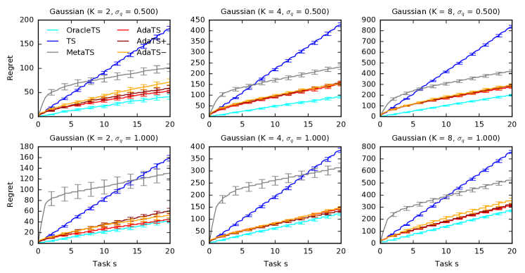
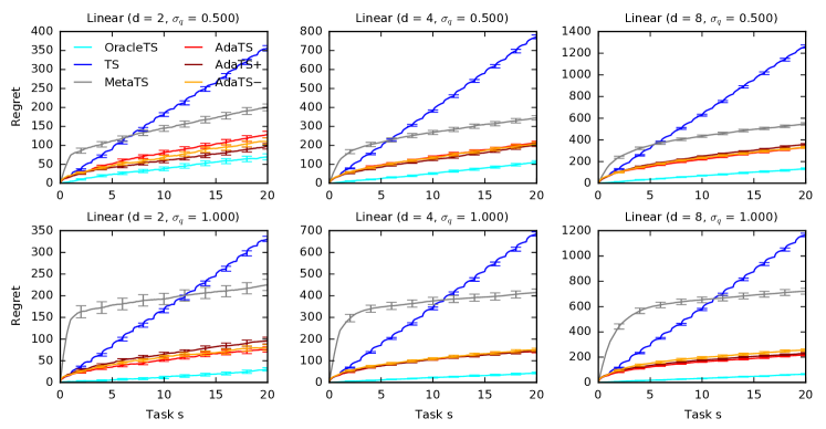
This section extends experiments in Section 5 in three aspects. First, we show the Gaussian bandit with $K\in\left\{2,4,8\right\}$ arms. Second, we show the linear bandit with $d\in\left\{2,4,8\right\}$ dimensions. Third, we implement $\tt AdaTS$ with a misspecified meta-prior.

Our results are reported in Figures 4 and 5. The setup of this experiment is the same as in Figure 2, and it confirms all earlier findings. We also experiment with two variants of misspecified $\tt AdaTS$. In $\tt AdaTS^{+}$, the meta-prior width is widened to $3\sigma_{q}$. This represents an overoptimistic agent. In $\tt AdaTS^{-}$, the meta-prior width is reduced to $\sigma_{q}/3$. This represents a conservative agent. We observe that this misspecification has no major impact on the regret of $\tt AdaTS$, which attests to its robustness.

E.2 Online One-Versus-All Classification Experiments

Figure 6: $\tt AdaTS$ in two meta-learning problems of digit classification from MNIST. On the top, we plot the cumulative regret as it accumulates over rounds within each task. Below we visualize the average digit, corresponding to the pulled arms in round $1$ of the tasks.

Figure 7: $\tt AdaTS$ in two meta-learning problems of character classification from Omniglot. On the top, we plot the cumulative regret as it accumulates over rounds within each task. Below we visualize the average character, corresponding to the pulled arms in round $1$ of the tasks.

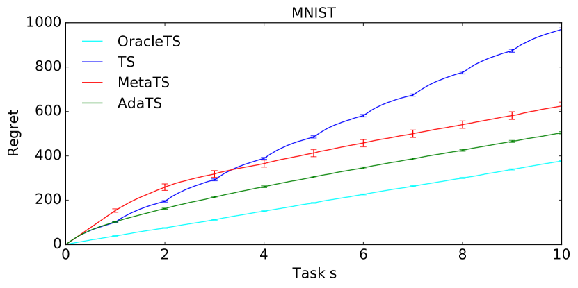
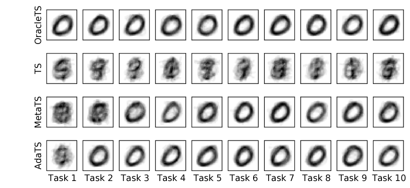
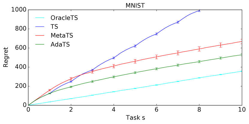
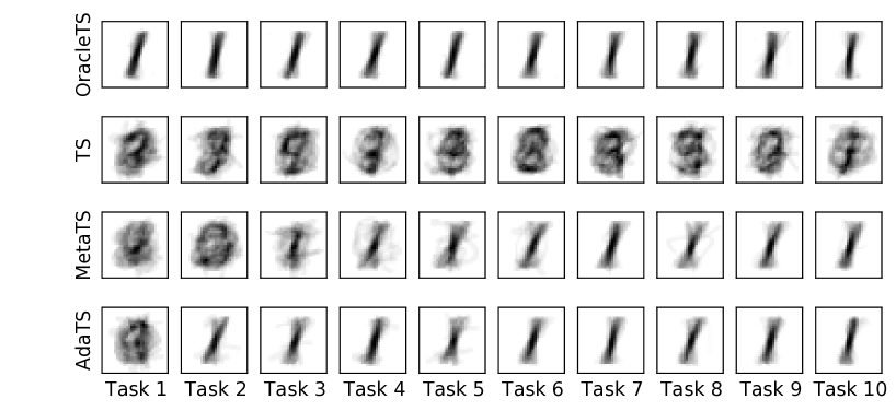
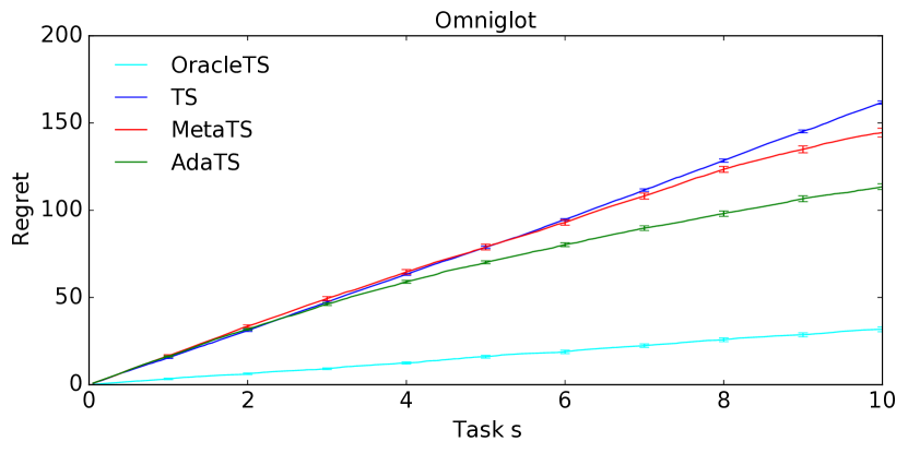
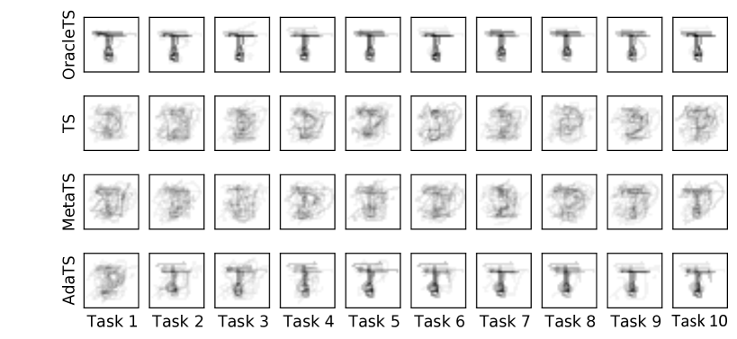
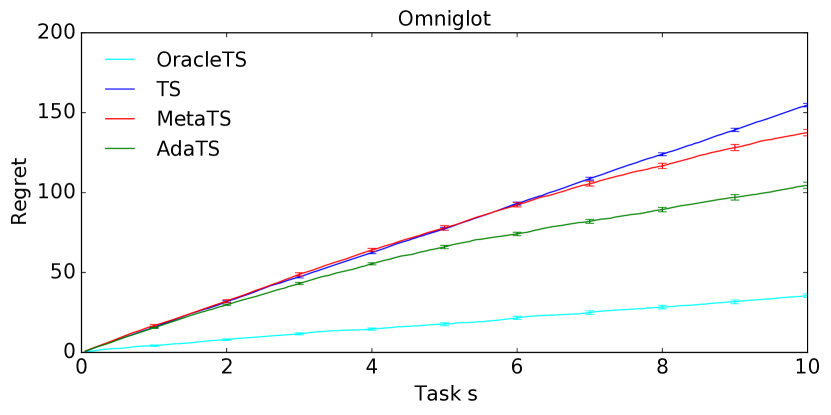
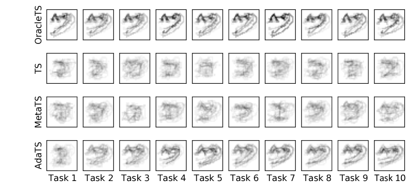
We consider online classification on two real-world datasets, which are commonly used in meta-learning. The problem is cast as a multi-task linear bandit with Bernoulli rewards. Specifically, we have a sequence of image classification tasks where one class is selected randomly to be positive. In each task, at every round, $K$ random images are selected as the arms and the goal is to pull the arm corresponding to an image from the positive class. The reward of an image from the positive class is $\mathrm{Ber}(0.9)$ and for all other classes is $\mathrm{Ber}(0.1)$. Dataset-specific settings are as follows:

1. MNIST [32]: The dataset contains $60\,000$ images of handwritten digits, which we split into equal-size training and test sets. We down-sample each image to $d=49$ features and then use these as arm features. The training set is used to estimate $\mu_{0}$ and $\Sigma_{0}$ for each digit. The bandit algorithms are evaluated on the test set. In each simulation, we have $m=10$ tasks with horizon $n=200$ and $K=30$ arms.

2. Omniglot [30]: The dataset contains $1\,623$ different handwritten characters from $50$ different alphabets. This is an extremely challenging dataset because we have only $20$ human-drawn images per character. Therefore, it is important to adapt quickly. We train a $4$-layer CNN to extract $d=64$ features using characters from $30$ alphabets. The remaining $20$ alphabets are split into equal-size training and test sets, with $10$ images per character in each. The training set is used to estimate $\mu_{0}$ and $\Sigma_{0}$ for each character. The bandit algorithms are evaluated on the test set. In each simulation, we have $m=10$ tasks with horizon $n=10$ and $K=10$ arms. We guarantee that at least one character from the positive class is among the $K$ arms.

In all problems, the meta-prior is $\mathcal{N}(\mathbf{0},I_{d})$ and the reward noise is $\sigma=0.1$. We compare $\tt AdaTS$ with the same three baselines as in Section 5, repeat all experiments $20$ times, and report the results in Figures 6 and 7. Along with the cumulative regret, we also visualize the average digit / character corresponding to the pulled arms in round $1$ of each task. We observe that $\tt AdaTS$ learns a very good meta-parameter $\mu_{*}$ almost instantly, since its average digit / character in task $2$ already resembles the unknown highly-rewarding digit / character. This happens even in Omniglot, where the horizon of each task is only $n=10$ rounds. Note that the meta-prior was not selected in any dataset-specific way. The fact that $\tt AdaTS$ still works well attests to the robustness of our method.

References

- Abbasi-Yadkori et al. [2011] Yasin Abbasi-Yadkori, David Pal, and Csaba Szepesvari. Improved algorithms for linear stochastic bandits. In Advances in Neural Information Processing Systems 24, pages 2312–2320, 2011.
- Agrawal and Goyal [2012] Shipra Agrawal and Navin Goyal. Analysis of Thompson sampling for the multi-armed bandit problem. In Proceeding of the 25th Annual Conference on Learning Theory, pages 39.1–39.26, 2012.
- Agrawal and Goyal [2013] Shipra Agrawal and Navin Goyal. Thompson sampling for contextual bandits with linear payoffs. In Proceedings of the 30th International Conference on Machine Learning, pages 127–135, 2013.
- Auer et al. [2002] Peter Auer, Nicolo Cesa-Bianchi, and Paul Fischer. Finite-time analysis of the multiarmed bandit problem. Machine Learning, 47:235–256, 2002.
- Azar et al. [2013] Mohammad Gheshlaghi Azar, Alessandro Lazaric, and Emma Brunskill. Sequential transfer in multi-armed bandit with finite set of models. In Advances in Neural Information Processing Systems 26, pages 2220–2228, 2013.
- Bastani et al. [2019] Hamsa Bastani, David Simchi-Levi, and Ruihao Zhu. Meta dynamic pricing: Transfer learning across experiments. CoRR, abs/1902.10918, 2019. URL https://arxiv.org/abs/1902.10918.
- Baxter [1998] Jonathan Baxter. Theoretical models of learning to learn. In Learning to Learn, pages 71–94. Springer, 1998.
- Baxter [2000] Jonathan Baxter. A model of inductive bias learning. Journal of Artificial Intelligence Research, 12:149–198, 2000.
- Boutilier et al. [2020] Craig Boutilier, Chih-Wei Hsu, Branislav Kveton, Martin Mladenov, Csaba Szepesvari, and Manzil Zaheer. Differentiable meta-learning of bandit policies. In Advances in Neural Information Processing Systems 33, 2020.
- Cella et al. [2020] Leonardo Cella, Alessandro Lazaric, and Massimiliano Pontil. Meta-learning with stochastic linear bandits. In Proceedings of the 37th International Conference on Machine Learning, 2020.
- Chapelle and Li [2012] Olivier Chapelle and Lihong Li. An empirical evaluation of Thompson sampling. In Advances in Neural Information Processing Systems 24, pages 2249–2257, 2012.
- Chen et al. [2013] Wei Chen, Yajun Wang, and Yang Yuan. Combinatorial multi-armed bandit: General framework, results and applications. In Proceedings of the 30th International Conference on Machine Learning, pages 151–159, 2013.
- Chen et al. [2014] Wei Chen, Yajun Wang, and Yang Yuan. Combinatorial multi-armed bandit and its extension to probabilistically triggered arms. CoRR, abs/1407.8339, 2014. URL http://arxiv.org/abs/1407.8339.
- Dani et al. [2008] Varsha Dani, Thomas Hayes, and Sham Kakade. Stochastic linear optimization under bandit feedback. In Proceedings of the 21st Annual Conference on Learning Theory, pages 355–366, 2008.
- Deshmukh et al. [2017] Aniket Anand Deshmukh, Urun Dogan, and Clayton Scott. Multi-task learning for contextual bandits. In Advances in Neural Information Processing Systems 30, pages 4848–4856, 2017.
- Duan et al. [2016] Yan Duan, John Schulman, Xi Chen, Peter Bartlett, Ilya Sutskever, and Pieter Abbeel. RL2: Fast reinforcement learning via slow reinforcement learning. CoRR, abs/1611.02779, 2016. URL http://arxiv.org/abs/1611.02779.
- Finn et al. [2017] Chelsea Finn, Pieter Abbeel, and Sergey Levine. Model-agnostic meta-learning for fast adaptation of deep networks. In Proceedings of the 34th International Conference on Machine Learning, pages 1126–1135, 2017.
- Finn et al. [2018] Chelsea Finn, Kelvin Xu, and Sergey Levine. Probabilistic model-agnostic meta-learning. In Advances in Neural Information Processing Systems 31, pages 9537–9548, 2018.
- Gai et al. [2012] Yi Gai, Bhaskar Krishnamachari, and Rahul Jain. Combinatorial network optimization with unknown variables: Multi-armed bandits with linear rewards and individual observations. IEEE/ACM Transactions on Networking, 20(5):1466–1478, 2012.
- Gelman et al. [2013] Andrew Gelman, John Carlin, Hal Stern, David Dunson, Aki Vehtari, and Donald Rubin. Bayesian Data Analysis. Chapman & Hall, 2013.
- Gentile et al. [2014] Claudio Gentile, Shuai Li, and Giovanni Zappella. Online clustering of bandits. In Proceedings of the 31st International Conference on Machine Learning, pages 757–765, 2014.
- Hong et al. [2020] Joey Hong, Branislav Kveton, Manzil Zaheer, Yinlam Chow, Amr Ahmed, and Craig Boutilier. Latent bandits revisited. In Advances in Neural Information Processing Systems 33, 2020.
- Hsu et al. [2019] Chih-Wei Hsu, Branislav Kveton, Ofer Meshi, Martin Mladenov, and Csaba Szepesvari. Empirical Bayes regret minimization. CoRR, abs/1904.02664, 2019. URL http://arxiv.org/abs/1904.02664.
- Kuleshov and Precup [2014] Volodymyr Kuleshov and Doina Precup. Algorithms for multi-armed bandit problems. CoRR, abs/1402.6028, 2014. URL http://arxiv.org/abs/1402.6028.
- Kveton et al. [2014] Branislav Kveton, Zheng Wen, Azin Ashkan, Hoda Eydgahi, and Brian Eriksson. Matroid bandits: Fast combinatorial optimization with learning. In Proceedings of the 30th Conference on Uncertainty in Artificial Intelligence, pages 420–429, 2014.
- Kveton et al. [2015] Branislav Kveton, Zheng Wen, Azin Ashkan, and Csaba Szepesvari. Tight regret bounds for stochastic combinatorial semi-bandits. In Proceedings of the 18th International Conference on Artificial Intelligence and Statistics, 2015.
- Kveton et al. [2020] Branislav Kveton, Martin Mladenov, Chih-Wei Hsu, Manzil Zaheer, Csaba Szepesvari, and Craig Boutilier. Differentiable meta-learning in contextual bandits. CoRR, abs/2006.05094, 2020. URL http://arxiv.org/abs/2006.05094.
- Kveton et al. [2021] Branislav Kveton, Mikhail Konobeev, Manzil Zaheer, Chih-Wei Hsu, Martin Mladenov, Craig Boutilier, and Csaba Szepesvari. Meta-Thompson sampling. In Proceedings of the 38th International Conference on Machine Learning, 2021.
- Lai and Robbins [1985] T. L. Lai and Herbert Robbins. Asymptotically efficient adaptive allocation rules. Advances in Applied Mathematics, 6(1):4–22, 1985.
- Lake et al. [2015] Brenden M Lake, Ruslan Salakhutdinov, and Joshua B Tenenbaum. Human-level concept learning through probabilistic program induction. Science, 350(6266):1332–1338, 2015.
- Lattimore and Szepesvari [2019] Tor Lattimore and Csaba Szepesvari. Bandit Algorithms. Cambridge University Press, 2019.
- LeCun et al. [2010] Yann LeCun, Corinna Cortes, and CJ Burges. Mnist handwritten digit database. ATT Labs [Online]. Available: http://yann.lecun.com/exdb/mnist, 2, 2010.
- Lu and Van Roy [2019] Xiuyuan Lu and Benjamin Van Roy. Information-theoretic confidence bounds for reinforcement learning. In Advances in Neural Information Processing Systems, volume 32, 2019.
- Maes et al. [2012] Francis Maes, Louis Wehenkel, and Damien Ernst. Meta-learning of exploration/exploitation strategies: The multi-armed bandit case. In Proceedings of the 4th International Conference on Agents and Artificial Intelligence, pages 100–115, 2012.
- Min et al. [2020] Seungki Min, Ciamac Moallemi, and Daniel Russo. Policy gradient optimization of Thompson sampling policies. CoRR, abs/2006.16507, 2020. URL http://arxiv.org/abs/2006.16507.
- Russo and Van Roy [2014] Daniel Russo and Benjamin Van Roy. Learning to optimize via posterior sampling. Mathematics of Operations Research, 39(4):1221–1243, 2014.
- Russo et al. [2018] Daniel Russo, Benjamin Van Roy, Abbas Kazerouni, Ian Osband, and Zheng Wen. A tutorial on Thompson sampling. Foundations and Trends in Machine Learning, 11(1):1–96, 2018.
- Thompson [1933] William R. Thompson. On the likelihood that one unknown probability exceeds another in view of the evidence of two samples. Biometrika, 25(3-4):285–294, 1933.
- Thrun [1996] Sebastian Thrun. Explanation-Based Neural Network Learning - A Lifelong Learning Approach. PhD thesis, University of Bonn, 1996.
- Thrun [1998] Sebastian Thrun. Lifelong learning algorithms. In Learning to Learn, pages 181–209. Springer, 1998.
- Vermorel and Mohri [2005] Joannes Vermorel and Mehryar Mohri. Multi-armed bandit algorithms and empirical evaluation. In Proceedings of the 16th European Conference on Machine Learning, pages 437–448, 2005.
- Wen et al. [2015] Zheng Wen, Branislav Kveton, and Azin Ashkan. Efficient learning in large-scale combinatorial semi-bandits. In Proceedings of the 32nd International Conference on Machine Learning, 2015.
- Yang et al. [2020] Jiaqi Yang, Wei Hu, Jason Lee, and Simon Du. Provable benefits of representation learning in linear bandits. CoRR, abs/2010.06531, 2020. URL http://arxiv.org/abs/2010.06531.
- Yang and Toni [2020] Kaige Yang and Laura Toni. Differentiable linear bandit algorithm. CoRR, abs/2006.03000, 2020. URL http://arxiv.org/abs/2006.03000.