NMR relaxation rates of quadrupolar aqueous ions from classical molecular dynamics using force-field specific Sternheimer factors

Abstract

The nuclear magnetic resonance (NMR) relaxation of quadrupolar nuclei is governed by the electric field gradient (EFG) fluctuations at their position. In classical molecular dynamics (MD), the electron cloud contribution to the EFG can be included via the Sternheimer approximation, in which the full EFG at the nucleus that can be computed using quantum density functional theory (DFT) is considered to be proportional to that arising from the external, classical charge distribution. In this work, we systematically assess the quality of the Sternheimer approximation as well as the impact of the classical force field (FF) on the NMR relaxation rates of aqueous quadrupolar ions at infinite dilution. In particular, we compare the rates obtained using an ab initio parametrized polarizable FF, a recently developed empirical FF with scaled ionic charges and a simple empirical non-polarizable FF with formal ionic charges. Surprisingly, all three FFs considered yield good values for the rates of smaller and less polarizable solutes (Li⁺, Na⁺, K⁺, Cl^-), provided that a model-specific Sternheimer parametrization is employed. Yet, the polarizable and scaled charge FFs yield better estimates for divalent and more polarizable species (Mg²⁺, Ca²⁺, Cs⁺). We find that a linear relationship between the quantum and classical EFGs holds well in all of the cases considered, however, such an approximation often leads to quite large errors in the resulting EFG variance, which is directly proportional to the computed rate. We attempted to reduce the errors by including first order nonlinear corrections to the EFG, yet no clear improvement for the resulting variance has been found. The latter result indicates that more refined methods for determining the EFG at the ion position, in particular those that take into account the instantaneous atomic environment around an ion, might be necessary to systematically improve the NMR relaxation rate estimates in classical MD.

1 Introduction

In a typical nuclear magnetic resonance (NMR) experiment, the nuclei with spin $I\geq 1$ predominantly relax through the quadrupolar mechanism that couples the quadrupolar moment of the nucleus $eQ$ with the electric field gradient (EFG) $V_{\alpha\beta}$ at its position ¹. Thus, the description of quadrupolar NMR relaxation is pertinent to the majority of alkaline metal, alkaline earth metal, and halide ions, that are species of considerable chemical, technological, and biological interest (${}^{7}{\rm Li}^{+}$, ${}^{23}{\rm Na}^{+}$, ${}^{39}{\rm K}^{+}$, ${}^{25}{\rm Mg}^{2+}$, ${}^{35}{\rm Cl}^{-}$, etc). During an NMR experiment, nuclear magnetic moments precess with the characteristic Larmor frequency $\omega_{0}=\gamma B_{0}$ where $\gamma$ is the gyromagnetic ratio of a given nucleus and $B_{0}$ is the external magnetic field. Provided that the typical molecular time scale $\tau$ over which the EFG decorrelates is small compared to $1/\omega_{0}$ ($\omega_{0}\tau\ll 1$, the so-called extreme narrowing regime), the magnetization along both the longitudinal and transverse directions of $B_{0}$ decays exponentially with equal rate constants $1/T_{1}$ and $1/T_{2}$, the spin-lattice and spin-spin relaxation rates, respectively. The latter quantities can be then computed as follows^{1, 2}:

$$\frac{1}{T_{1}}=\frac{1}{T_{2}}=\frac{1}{20}\frac{2I+3}{I^{2}(2I-1)}\left(\frac{eQ}{\hbar}\right)^{2}\int_{0}^{\infty}{\rm d}t\,\langle{\mathbf{V}}(t)\,{:}{\mathbf{V}}(0)\rangle,$$ (1)

where $\hbar$ is the reduced Planck constant, ${\mathbf{V}}$ is the total EFG tensor at the nucleus position, and $\langle{\mathbf{V}}(t)\,{:}{\mathbf{V}}(0)\rangle\equiv\langle\sum_{\alpha,\beta}V_{\alpha\beta}(t)V_{\alpha\beta}(0)\rangle$ ($\alpha$ and $\beta$ run over the three Cartesian components) is the EFG autocorrelation function (ACF), $C_{\rm EFG}(t)$. Finally, $\langle\dots\rangle$ in Eq. (1) denotes an average in the canonical ensemble (fixed number of particles $N$, volume $V$ and temperature $T$), without an imposed magnetic field. The isotropic character of the equilibrium system permits to have such simple formulation of Eq. (1) that is rooted in the linear response theory.

The estimation of the EFG ACF requires both a good sampling of the microscopic dynamics of the system and an accurate computation of the EFG along the trajectory. In principle, ab initio molecular dynamics (MD) can provide both features^{3, 4, 5}, yet the entailed computational cost often limits the ability to converge the corresponding ACF with sufficient accuracy for a reliable estimate of its integral⁶. This motivated the use of classical MD to sample configurations over the relevant time scales, yet the accurate estimation of the EFG at the nucleus position has remained a formidable challenge in classical MD^{7, 8, 9, 2, 10, 11}. Such challenge comes from the fact that the dominant contribution to the total EFG $V_{\alpha\beta}$ is due to the intraatomic electronic charge distribution around a nucleus that is not available in atomistic classical models and is even difficult to obtain accurately with electronic structure calculations. Yet, quantum density functional theory (DFT) allows to quite accurately compute EFGs for main group elements and some transition metals¹², although a complete understanding of the solvation effects on the EFGs has remained challenging. In the case of monoatomic ions, the widespread electrostatic models of the EFG relaxation^{13, 14, 15, 16} consider that the EFG at the nucleus is created by the inhomogeneous distribution of external charges that polarize the electronic cloud of the given ion. Consequently, a linear relation between the total $V_{\alpha\beta}$ and external $V^{\rm ext}_{\alpha\beta}$ EFG is often assumed, yielding the so-called Sternheimer approximation¹⁷:

$$\mathbf{V}\simeq(1+\gamma)\mathbf{V}_{\rm ext},$$ (2)

where the constant $\gamma$ is the Sternheimer (anti-)shielding factor ^{18, 19} that is usually large, $\gamma\gg 1$ (note that Eq. (2) uses a different sign convention for $\gamma$ than in Refs. ^{18, 19, 20}). While the exact external charge distribution that comes from solvent molecules and gives rise to $\mathbf{V}_{\rm ext}$ is generally unknown, in classical MD it is approximated by a simpler distribution corresponding to the charges used to compute electrostatic interactions. Following previous work, we will assume that $V_{\alpha\beta}^{\rm ext}$ in Eq. (2) is due to the external, force-field based charge distribution readily available in classical MD, whereas a specific value of $\gamma$ can be determined using auxiliary quantum-mechanical calculations for the system at hand. For instance, the Sternheimer factors can be derived using a perturbation theory in the long-range approximation^{18, 19} (usually denoted as $\gamma_{\infty}$), in which the polarization of a spherical electron cloud around an ion is due to a distant charge distribution. Nevertheless, the values of $\gamma_{\infty}$ that do not capture polarization effects from solvent-solute interactions were shown to differ considerably from that of ions in aqueous solutions ¹⁰. Inserting Eq. (2) into Eq. (1), the expression (1) for the relaxation rate can be recast as

$$\frac{1}{T_{1}}=C_{Q}(1+\gamma)^{2}\langle\mathbf{V}_{\rm ext}^{2}\rangle\tau_{c},$$ (3)

where $C_{Q}\equiv\frac{1}{20}\frac{2I+3}{I^{2}(2I-1)}\left(\frac{eQ}{\hbar}\right)^{2}$ is an ion specific constant, $\langle\mathbf{V}_{\rm ext}^{2}\rangle\equiv\langle{\mathbf{V}}_{\rm ext}(0)\,{:}{\mathbf{V}}_{\rm ext}(0)\rangle$ is the variance of the external EFG, and $\tau_{c}$ is an effective correlation time

$$\tau_{c}=\langle\mathbf{V}_{\rm ext}^{2}\rangle^{-1}\,\int_{0}^{\infty}{\rm d}t\,\langle{\mathbf{V}}_{\rm ext}(t)\,{:}{\mathbf{V}}_{\rm ext}(0)\rangle\;.$$ (4)

Equations (3) and (4) serve as a starting point of the present work. Using a series of classical force fields (FFs) as described in detail below in Section 2, we simulate single ions dissolved in water to determine the variance of the external EFG $\langle\mathbf{V}_{\rm ext}^{2}\rangle$, the ACF of external EFG, and the effective correlation time $\tau_{c}$ (4). In line with the earlier work ¹⁰, we then determine the effective model-specific Sternheimer factors $\gamma_{\rm eff}$ by comparing the EFG at the ion position obtained from classical MD to that from ab initio (AI) DFT calculations on a set of configurations generated with classical FFs. Finally, the resulting combination of $\langle\mathbf{V}_{\rm ext}^{2}\rangle$, $\tau_{c}$, and $\gamma_{\rm eff}$, and ionic parameters ($I$, $eQ$) allows to consistently determine the NMR relaxation rate $1/T_{1}$ as given by Eq. (3).

In this work we aim to address the following questions: $(i)$ Can accurate quadrupolar NMR relaxation rates be obtained from classical MD simulations with various degrees of sophistication, provided that the electronic contribution to the EFG is included via AI-parametrized, model-specific Sternheimer factors that capture local solvent-solute interactions? $(ii)$ How well does the Sternheimer approximation describe the AI-derived EFGs at the ion position and can the incorporation of non-linear effects improve the predictions of the Sternheimer model? $(iii)$ How do the Sternheimer factors depend on the structure of the hydration shell around an ion? $(iv)$ To what extent the treatment of polarizability in classical MD impacts the obtained NMR relaxation rates? The rest of the article is therefore structured as follows. In Section 2, we describe the details of our classical MD and quantum DFT simulations. In Section 3, we validate the Sternheimer approximation for different ions using a series of classical FFs and consider its possible extensions as well as dependence on the hydration shell structure around an ion. In Section 4, we consider the EFG relaxation at the nucleus position of various alkali metal, alkaline earth metal, and halide ions with the employed FFs to determine their quadrupolar NMR relaxation rates at infinite dilution, before concluding in Section 5.

2 Simulation details

To systematically assess the impact of the underlying classical model on the resulting NMR relaxation rates, we investigated three FFs for aqueous electrolyte solutions that differ in terms of their parametrization strategy (AI- vs. empirically-parametrized), the geometry of water molecules, and the treatment of electronic polarizability: $(i)$ the explicitly polarizable ion model²¹ (PIM) based on the rigid four site Dang-Chang water²²; $(ii)$ the Madrid-2019 model²³ with scaled ionic charges based on the rigid four site TIP4P/2005 water²⁴; $(iii)$ the Amber-14 FF ²⁵, ²⁶, ²⁷, ²⁸ based on the rigid three site SPC/E water²⁹ and formal ionic charges. In both Dang-Chang and TIP4P/2005 rigid water models, the molecules carry an additional massless M-site that bears the negative charge and lies along the bisector of the HOH bond angle. In addition, the M-site of the Dang-Chang water carries an induced dipole moment in the PIM, as discussed further below.

The total potential energy of the PIM is given by²¹:

$$U^{\rm PIM}_{\rm tot}=U_{\rm charge}+U_{\rm disp}+U_{\rm rep}+U_{\rm LJ}+U_{\rm pol}.$$ (5)

In Eq. (5), $U_{\rm charge}$ stands for the Coulomb interaction between charges $q^{i}$ and $q^{j}$ separated by the distance $r_{ij}$ (unless otherwise specified, atomic units are employed throughout the article):

$$U_{\rm charge}=\sum_{i<j}\frac{q^{i}q^{j}}{r_{ij}}.$$ (6)

Note that in the PIM ions bear formal charges (+1, -1, +2), while the sites in Dang-Chang water molecules bear partial charges ($q_{\rm H}=+0.5190$, $q_{\rm O}=0$, $q_{\rm M}=-2q_{\rm H}$). $U_{\rm disp}$ is the dispersion potential:

$$U_{\rm disp}=-\sum_{i<j}\left[f^{ij}_{6}(r_{ij})\frac{C^{ij}_{6}}{r_{ij}^{6}}+f^{ij}_{8}(r_{ij})\frac{C^{ij}_{8}}{r_{ij}^{8}}\right],$$ (7)

where $f^{ij}_{n}=1-\exp\left({-b^{ij}_{D}r_{ij}}\right)\sum_{k=0}^{n}\frac{\left(b^{ij}_{D}r_{ij}\right)^{k}}{k!}$ are the short-range corrections of the Tang-Toennies type. $U_{\rm rep}$ captures the repulsive part of ion-ion and ion-water interactions:

$$U_{\rm rep}=\sum_{i<j}A^{ij}e^{-B^{ij}r_{ij}}.$$ (8)

In addition, instead of $U_{\rm disp}+U_{\rm rep}$ in Eqs. (7) and (8), the Lennard-Jones potential $U_{\rm LJ}$ is used to describe the water-water repulsion and dispersion in the Dang-Chang water model:

$$U_{\rm LJ}=\sum_{i<j}4\epsilon_{ij}\left[\left(\frac{\sigma_{ij}}{r_{ij}}\right)^{12}-\left(\frac{\sigma_{ij}}{r_{ij}}\right)^{6}\right].$$ (9)

Finally, the polarization energy $U_{\rm pol}$ describes electrostatic many-body effects that are included through induced dipoles ${\boldsymbol{\mu}}^{i}$:

$$U_{\rm pol}=\sum_{i}\frac{|{\boldsymbol{\mu}}^{i}|^{2}}{2\alpha^{i}}+\sum_{i,j}\left[\left(q^{i}\mu^{j}_{\alpha}g^{ij}(r_{ij})-q^{j}\mu^{i}_{\alpha}g^{ji}(r_{ij})\right)T_{ij}^{\alpha}-\mu_{\alpha}^{i}\mu_{\beta}^{j}T_{ij}^{\alpha\beta}\right],$$ (10)

where Einstein summation is used for Cartesian components $\alpha$ and $\beta$, $\alpha^{i}$ is the polarizability of the $i$-th atom, $T_{ij}^{\alpha}=\partial_{\alpha}(1/r_{ij})$ and $T_{ij}^{\alpha\beta}=\partial_{\alpha}\partial_{\beta}(1/r_{ij})$ are multipole interaction tensors, and $g^{ij}(r_{ij})=1-c^{ij}\exp\left({-b^{ij}r_{ij}}\right)\sum_{k=0}^{4}\frac{\left(b^{ij}r_{ij}\right)^{k}}{k!}$ is a short-range Tang-Toennies correction. The induced dipoles are determined at every integration time step through minimization of $U_{\rm pol}$ in Eq. (10). In practice, the induced dipoles for cations in the PIM are neglected due to their quite small polarizability²¹. The induced dipole of a Dang-Chang water molecule is carried by the virtual M-site. All ion-ion, ion-water, and water-water interactions parameters in Eqs. (6), (7), (8), (9), and (10) were taken from Ref. 21.

The Madrid-2019²³ model for ions in aqueous solutions employs only $U_{\rm charge}$ (see Eq. (6)) and $U_{\rm LJ}$ (see Eq. (9)) to describe all interactions in the system:

$$U_{\rm tot}^{\rm Madrid-2019}=U_{\rm charge}+U_{\rm LJ},$$ (11)

where ions carry scaled charges (+0.85, -0.85, +1.70 for monovalent cations, monovalent anions and divalent cations, respectively) as an effective way to introduce the electronic polarizability of the medium, and sites on water molecules carry partial charges ($q_{\rm H}=+0.5564$, $q_{\rm O}=0$, $q_{\rm M}=-2q_{\rm H}$). The corresponding Lennard-Jones interaction parameters $\epsilon_{ij}$ and $\sigma_{ij}$ can be found in Ref. 23. Finally, the SPC/E-based Amber14 FF ^{25, 26, 27, 28} is similarly described with

$$U_{\rm tot}^{\rm Amber14}=U_{\rm charge}+U_{\rm LJ}$$ (12)

with formal ionic charges (+1, -1, +2) and the partial charges of the SPC/E water molecules ($q_{\rm H}=+0.4238$, $q_{\rm O}=-2q_{\rm H}$). The corresponding interaction parameters were taken from Refs. 25, 26, 27.

To mimic infinite dilution conditions, $N=256$ water molecules and 1 ion were simulated in a cubic box at density $\rho=0.997$ g/cm³ and temperature $T=298.15$ K that was maintained using the Nosé-Hoover chains thermostat^{30, 31, 32} with a time constant of 1 ps. Electrostatic interactions were treated using Ewald summation^{33, 34}. The cutoff for short-range interactions was set to the half of the box side length (close to 1 nm). Initially, arbitrary-oriented water molecules and an ion were randomly initialized on a lattice, then annealed at $T=1000$ K for 150 ps and subsequently equilibrated at $T=298.15$ K for another 150 ps. Such preparation protocol was followed by 5 independent production runs each of length 1 ns in the $NVT$ ensemble with an integration time step of 1 fs. The water molecules were made effectively rigid by integrating their equations of motion using the RATTLE³⁵ algorithm with precision $10^{-9}$. All classical MD simulations as well as the EFG calculations were performed with the MetalWalls package³⁶. In the case of PIM simulations, the induced dipoles were determined self-consistently using the conjugate gradient algorithm with tolerance $10^{-6}$. The computation of the EFG at the ion position due to point charges and point dipoles, with the latter contributing only in the case of PIM simulations, was implemented using Ewald summation^{33, 34} in the MetalWalls package (release version 21.06³⁷) and was performed at every integration time step. Finally, it is important to note that in the case of a non-electroneutral system, the trace of the classical EFG computed using the Ewald summation expressions³³ features a non-zero trace

$$\mathrm{Tr}\,\mathbf{V}_{\rm ext}=-\frac{4\pi}{V}q_{\rm tot},$$ (13)

where $q_{\rm tot}$ is the total charge of the simulation box and $V$ is its volume. To ensure that the final EFG is traceless, a third of (13) was subtracted from the diagonal EFG components before analysis. In addition, we verified that the resulting EFG ACFs are almost identical to those in a dilute, explicitly electroneutral system (see Supporting Fig. S1a and S1b). Finally, the EFG ACFs obtained from $NVE$ production runs are in excellent agreement with the ones in the $NVT$ ensemble (see Supporting Fig. S1c and S1d).

To determine effective Sternheimer factors, for each classical FF we additionally simulated a smaller system comprised of 64 water molecules and 1 ion using the same system parameters as discussed before. The smaller systems were prepared with the same protocol as the larger ones. Subsequently, we sampled 1000 configurations every 10 ps during a single $NVT$ production run to ensure a sufficient degree of decorrelation between two consecutive snapshots. These 1000 configurations from classical MD were used as an input for the DFT-based computations of the EFG in the condensed phase that include the electronic contribution. The DFT calculations were performed in the Quantum Espresso (QE) package³⁸ using the projected augmented wave (PAW) method to allow for an all-electron representation of the core region. ^{39, 40, 41}. The AI EFG at the ion position was evaluated with periodic boundary conditions using the QE-GIPAW package⁴². The self-consistent electron densities were obtained using the PBE functional⁴³ and a kinetic energy cutoff of 80 Ry. In the case of Li⁺, Na⁺, K⁺, Cl^-, Mg²⁺, Ca²⁺ ions we employed the norm-conserving pseudopotentials included in the GIPAW package⁴⁴, whereas for Cs⁺, Br^-, and I^- we used the PAW pseudopotentials from the pslibrary 1.0.0⁴⁵. Due to approximations involved in representing AI EFGs in the present approach, here we used the PBE functional for all ions, although more advanced functionals can provide a more accurate description of EFGs for larger and more polarizable species ^{12, 5}. In other words, the errors produced by the Sternheimer approximation (2) might considerably outweigh the ones associated with the use of a simpler DFT functional.

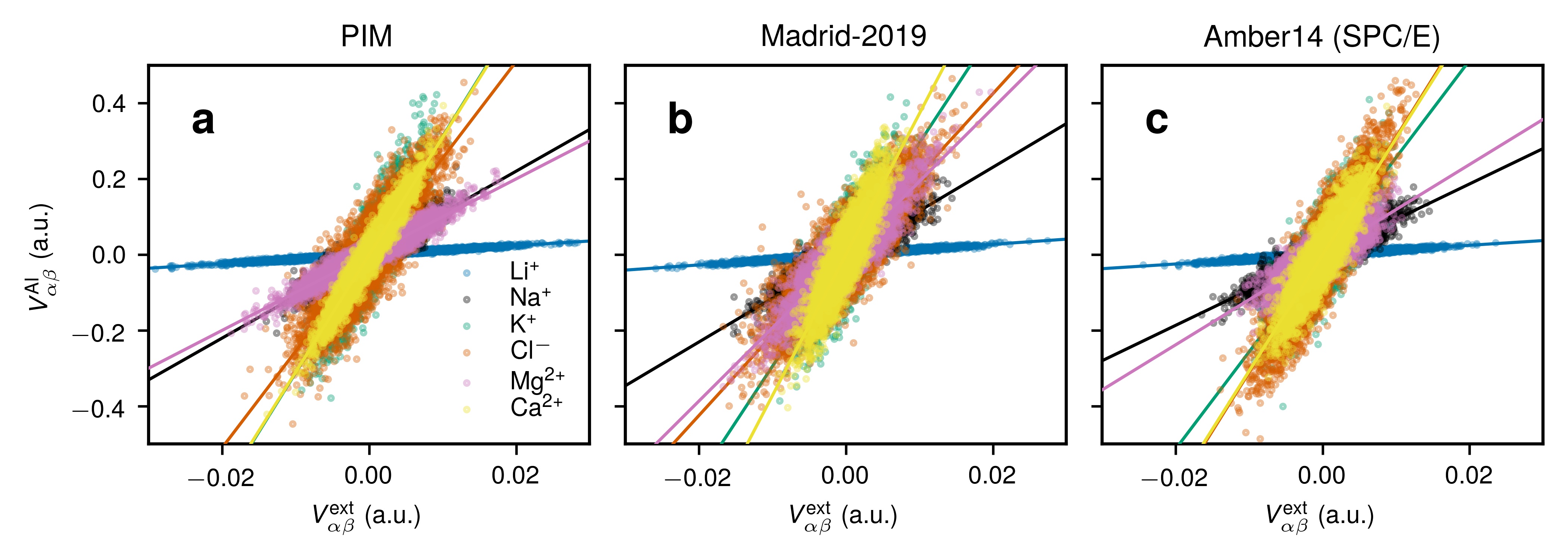
Figure 1: Validation of the Sternheimer approximation for different classical FFs. The EFG components obtained using classical MD, $V_{\alpha\beta}^{\rm ext}$, are plotted versus the ab initio ones, $V_{\alpha\beta}^{\rm AI}$, following the procedure explained in Section 2. A linear relationship between $V_{\alpha\beta}^{\rm AI}$ and $V_{\alpha\beta}^{\rm ext}$ is evident in all cases considered and allows to define an effective Sternheimer factor $V_{\alpha\beta}^{\rm AI}=(1+\gamma_{\rm eff})V_{\alpha\beta}^{\rm ext}$ for every model. The fits for $\gamma_{\rm eff}$ are shown with solid lines, whereas the obtained values of $\gamma_{\rm eff}$ are listed in Tab. 1. The results for Li⁺, Na⁺, K⁺, Cl^-, Mg²⁺, and Ca²⁺ ions are indicated with a different color shown in the legend of (a) (the legend is the same for all plots). Additional results for Cs⁺, Br^-, and I^- are shown in Supporting Fig. S2.

3 Sternheimer approximation

3.1 Effective Sternheimer factor

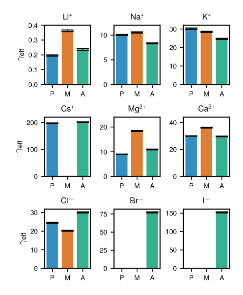
Figure 2: The effective Sternheimer factors for different quadrupolar nuclei at infinite dilution. For every ion, we indicate $\gamma_{\rm eff}$ for the PIM (P), the Madrid-2019 model (M), and Amber14 FF parameters for the SPC/E water and ions (A).

We first assess the validity of the Sternheimer approximation by comparing the EFGs obtained with classical MD simulations, $V_{\alpha\beta}^{\rm ext}$, to that from DFT GIPAW calculations, $V_{\alpha\beta}^{\rm AI}$, on a set of 1000 configurations. The results for Li⁺, Na⁺, K⁺, Cl^-, Mg²⁺, and Ca²⁺ ions, the parameters for which are available in all three FFs considered in this work, are shown in Fig. 1. Additional results for Cs⁺, Br^-, I^-, and Ca²⁺ ions can be found in Supporting Figs. S2 and S3. In agreement with earlier work¹⁰, we find that the linear relation $V_{\alpha\beta}^{\rm AI}\simeq(1+\gamma_{\rm eff})V_{\alpha\beta}^{\rm ext}$ holds well in all of the cases considered (that is, for all ions and FFs) and allows to determine effective model-dependent Sternheimer factors $\gamma_{\rm eff}$ using a linear fit (2). Note that here and in what follows we will distinguish between the effective Sternheimer factors $\gamma_{\rm eff}$ derived for a specific atomic environment and $\gamma_{\rm\infty}$ that are calculated using perturbation methods for model condensed phase environments or free ions in response to a distant charge distribution^{19, 20}. From the slope of the scatter plots in Fig. 1 and Supporting Fig. S2, we consistently find that $V_{\alpha\beta}^{\rm AI}$ responds positively to the EFG of the external (ionic) charge distribution, $V_{\alpha\beta}^{\rm ext}$, in the present approach, leading to the anti-shielding effect and strictly positive values of the obtained Sternheimer factors. This differs from the case of $\gamma_{\infty}$ for Li⁺ obtained via the Watson sphere model, which aimed at modeling a solid-like environment²⁰, that results in the shielding effect for the cation and a negative value of $\gamma_{\infty}$. Further below we will compare in more detail the values of $\gamma_{\rm eff}$ devised in this work and that of $\gamma_{\infty}$ from the Watson sphere model that were used in the early systematic study on the NMR relaxation rates of quadrupolar nuclei by Roberts and Schnitker².

Table 1: Effective Sternheimer factors $\gamma_{\rm eff}$ and corresponding prediction errors $\sigma(\mathbf{V}^{2})$ on the EFG variance (see Eq. (15)) obtained for different classical FFs. The values in parentheses indicate standard errors obtained using bootstrapping. The reference values of $\gamma_{\infty}$ correspond to the Watson sphere model on an ionic solid²⁰. Note that here the sign of $\gamma_{\infty}$ is opposite to the one in Ref. 20 to comply with the convention in Eq. (2).

Ion	$\gamma_{\infty}$	PIM		Madrid-2019		Amber14
		$\gamma_{\rm eff}$	$\sigma(\mathbf{V}^{2})$	$\gamma_{\rm eff}$	$\sigma(\mathbf{V}^{2})$	$\gamma_{\rm eff}$	$\sigma(\mathbf{V}^{2})$
Li+	-0.255	0.196(0.004)	0.20	0.362(0.006)	0.26	0.237(0.007)	0.29
Na+	5.452	10.02(0.11)	0.46	10.54(0.11)	0.46	8.34(0.09)	0.43
K+	21.782	30.21(0.32)	0.47	28.51(0.33)	0.47	24.67(0.29)	0.48
Cs+	110.81	196.7(1.0)	0.25	—	—	201.8(1.0)	0.26
Cl-	41.999	24.50(0.24)	0.42	20.25(0.22)	0.42	30.06(0.27)	0.39
Br-	85.517	—	—	—	—	77.16(0.65)	0.39
I-	162.42	—	—	—	—	152.1(1.3)	0.40
Mg2+	4.118	9.00(0.06)	0.36	18.34(0.17)	0.55	10.91(0.15)	0.56
Ca2+	18.791	30.02(0.13)	0.23	36.24(0.30)	0.36	29.73(0.23)	0.36

The comparison between $\gamma_{\rm eff}$ for different classical FFs are shown in Fig. 2, whereas explicit values are listed in Tab. 1 (the corresponding standard errors were estimated using bootstrapping). As expected, for the considered atomic species the effective Sternheimer factor increases with the number of electrons, indicating its dominant contribution to the total EFG at the nucleus position. In addition, certain quantitative differences are found when comparing $\gamma_{\rm eff}$ across the three classical FFs considered, highlighting the sensitivity of local polarization effects to the charge distribution around an ion and solute-solvent interactions. For the two smallest cations, Li⁺ and Mg²⁺, $\gamma_{\rm eff}$ in the Madrid-2019 model are larger by a factor $\approx$ 1.5–2 than those in the PIM and Amber14 FFs. A similar trend is found for Ca²⁺, however the magnitude of $\gamma_{\rm eff}^{\rm Madrid-2019}$ is bigger by a factor $\approx$ 1.2 when compared to the two other FFs. Smaller differences in $\gamma_{\rm eff}$ across models are seen for larger Na⁺, K⁺, and Cs⁺ cations. For the Cl^- anion, $\gamma_{\rm eff}$ for the Amber14 FF is larger by a factor $\approx$ 1.25–1.5 than those for the PIM and Madrid-2019 model.

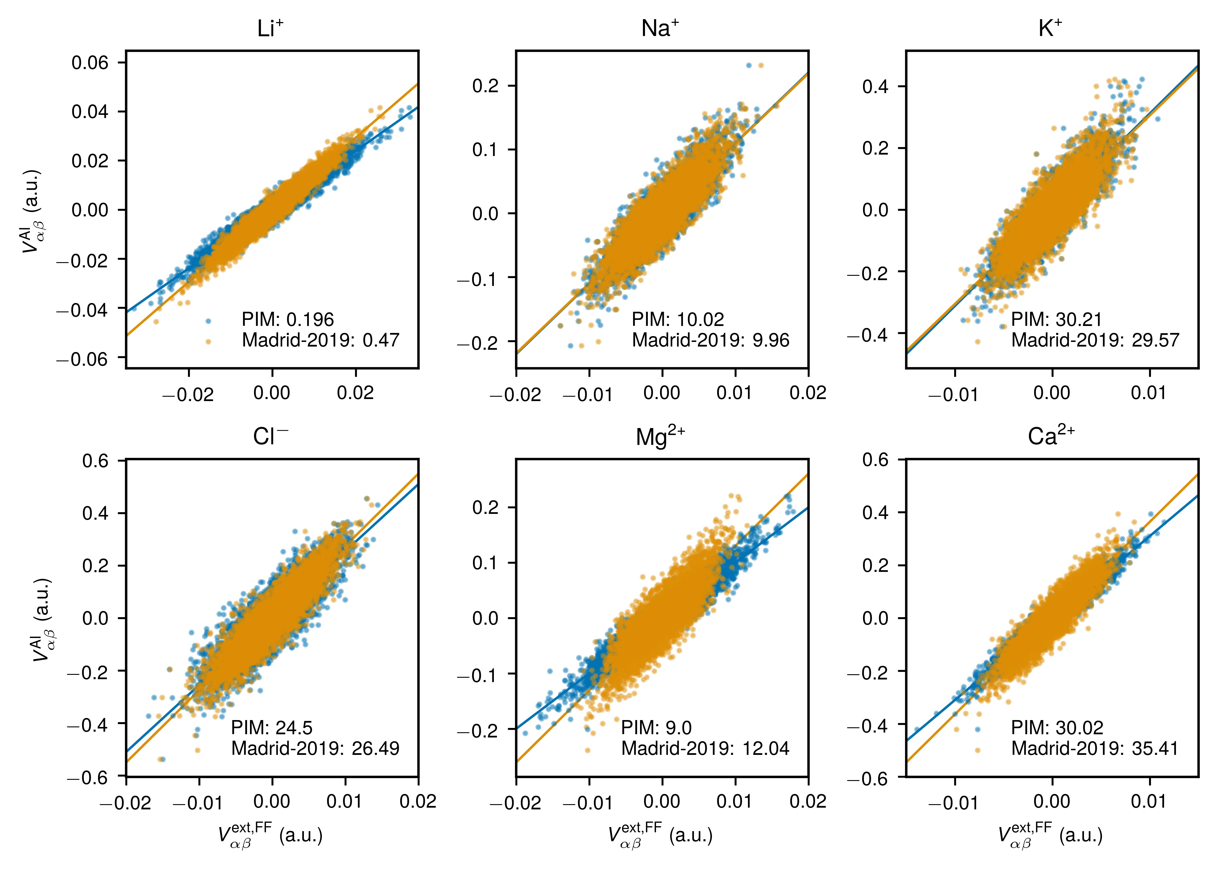
Figure S4: Effect of changing the representation of the charge distribution in the classical force field on the resulting effective Sternheimer factors in the PIM model for various ions. The AI EFGs $V_{\alpha\beta}^{\rm AI}$ obtained on the set of configurations generated using PIM dynamics are plotted against the external, force field specific EFG $V_{\alpha\beta}^{\rm ext,FF}$ as computed using the PIM (blue dots) or using the Madrid-2019 FF (yellow dots) on the same set of configurations. The resulting Sternheimer factors $\gamma_{\rm eff}$, $V_{\alpha\beta}^{\rm AI}=(1+\gamma_{\rm eff})V_{\alpha\beta}^{\rm ext,FF}$ are listed in the legends.

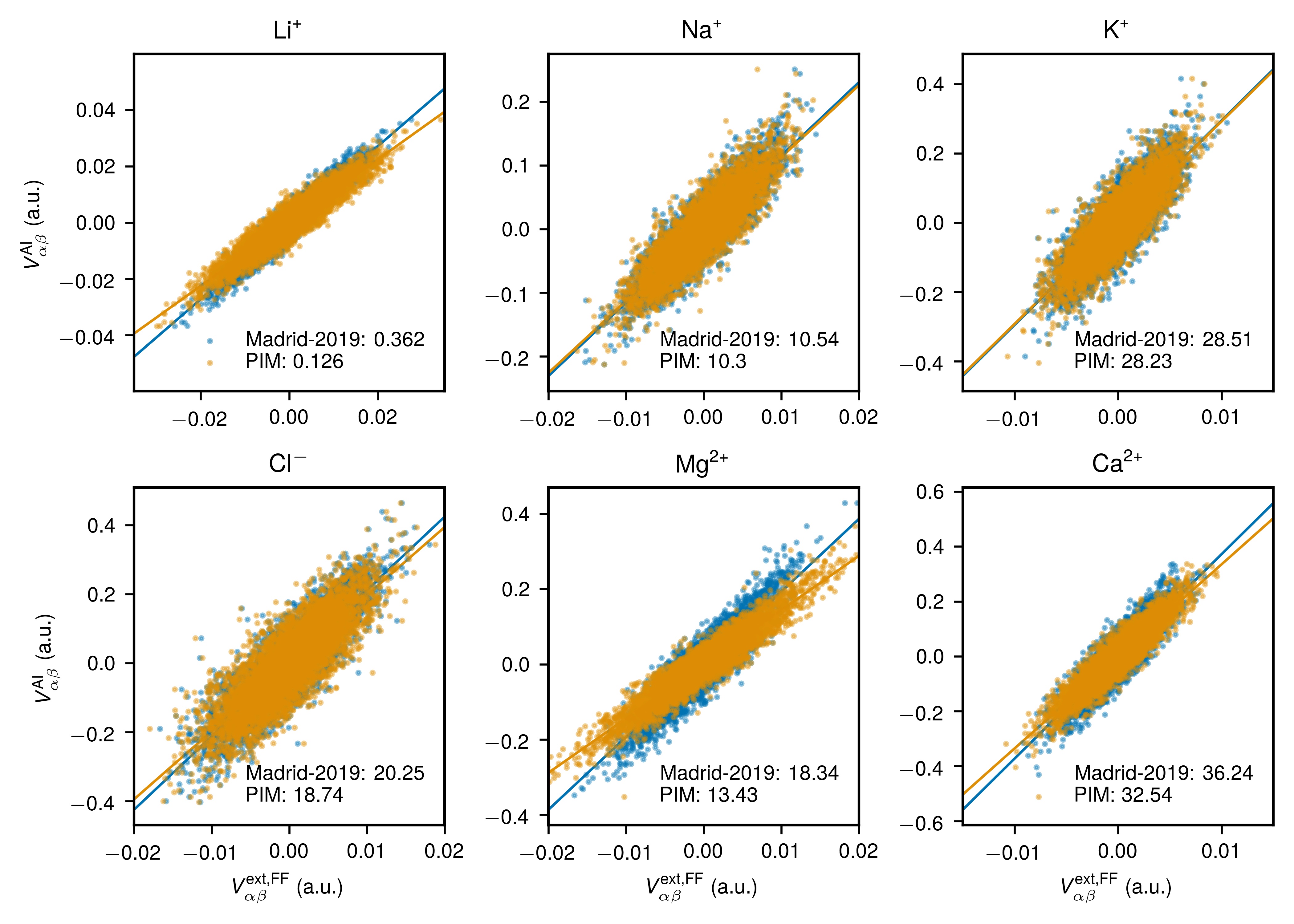
Figure S5: Effect of changing the representation of the charge distribution in the classical force field on the resulting effective Sternheimer factors in the Madrid-2019 model for various ions. The AI EFGs $V_{\alpha\beta}^{\rm AI}$ obtained on the set of configurations generated using Madrid-2019 dynamics are plotted against the external, force field specific EFG $V_{\alpha\beta}^{\rm ext,FF}$ as computed using the Madrid-2019 FF (blue dots) or using the PIM (yellow dots) on the same set of configurations. The resulting Sternheimer factors $\gamma_{\rm eff}$, $V_{\alpha\beta}^{\rm AI}=(1+\gamma_{\rm eff})V_{\alpha\beta}^{\rm ext,FF}$ are listed in the legends.

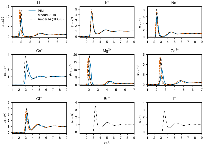
Figure S6: Ion-oxygen radial distribution functions in the PIM (solid blue lines), Madrid-2019 (dashed red lines), and Amber14 FF parameters for ions and SPC/E water (dotted black lines) for different ions at infinite dilution.

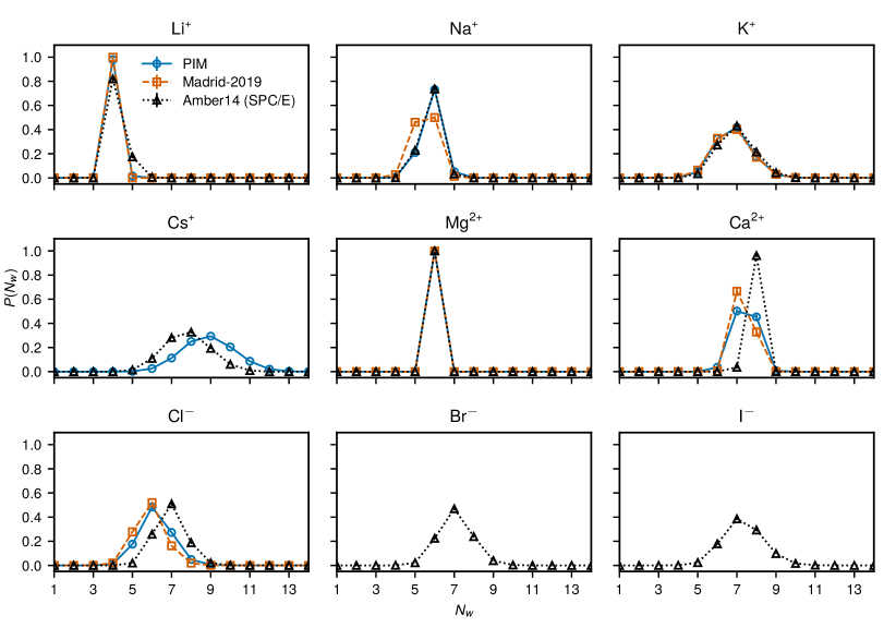
Figure S7: Probability of finding $N_{\rm w}$ water molecules in the first hydration shell of single ions in the PIM (blue open circles), the Madrid-2019 model (red open squares), and Amber14 FF parameters for ions and SPC/E water (black open triangles).

When the comparison is made across different FFs, two effects may play an important role: $(i)$ the representation of the charge density around an ion using different (partial) point charges and point dipoles (in polarizable models) on water molecules; $(ii)$ changes in the structure and dynamics of the solvation shell around an ion. Both effects can potentially influence $V_{\alpha\beta}^{\rm AI}$ and $V_{\alpha\beta}^{\rm ext}$, and therefore the computed value of $\gamma_{\rm eff}$. To assess the effect of charge density representation via distinct water point charges and dipoles, we have adopted the following strategy. First, we took 1000 system configurations that were used in the AI calculations of the Sternheimer factor for the PIM and recomputed the external EFGs using the point charges from the Madrid-2019 FF (this is possible thanks to the same TIP4P/2005 geometry of water molecules in these two FFs). The latter allowed us to calculate Sternheimer factors for configurations that were generated with the PIM dynamics but with point charges of the Madrid-2019 FF (Supporting Fig. S4). Interestingly, we find that such operation results in quite larger values of $\gamma_{\rm eff}$ for Li⁺, Mg²⁺, Ca²⁺ that become closer to the ones obtained consistently for the Madrid-2019 FF (Tab. 1). Yet, the values of $\gamma_{\rm eff}$ obtained after such a numerical experiment are not in quantitative agreement with those for the Madrid-2019 FF (Tab. 1), suggesting additional differences that stem from variations in the solvation shell structure in the two models at hand, which are highlighted in the difference in the ion-oxygen radial distribution functions and in the number of water molecules in the shell (Supporting Figs. S6 and S7, respectively). Furthermore, much smaller variations in $\gamma_{\rm eff}$ are found for Na⁺ and K⁺. In addition, $\gamma_{\rm eff}$ for Cl^- increases contrary to the corresponding value in the Madrid-2019 FF (Tab. 1). Consistently, opposite trends for $\gamma_{\rm eff}$ of Li⁺, Mg²⁺, Ca²⁺, and Cl^- are observed when the Sternheimer factors are calculated using configurations that were generated with the Madrid-2019 dynamics but with point charges and dipoles of the PIM (Supporting Fig. S5). In summary, the latter observations highlight the sensitivity of the obtained $\gamma_{\rm eff}$ to the charge density representation of the chosen water model. Further differences in $\gamma_{\rm eff}$ are likely caused by subtle variations in the solvation shell structure across the FFs (Supporting Figs. S6 and S7). For instance, the Amber14 FF features approximately one more molecule in the first solvation shell of the Cl^- anion on average as compared to the two other models (6.9 vs. 6.2 and 5.9, respectively, see Supporting Fig. S7 and Tab. S1), which can result in an enhanced polarization of the electronic cloud by hydrogen bonds donated by water for such an environment. Finally, the observed deviations in computed $\gamma_{\rm eff}$ across different classical FFs again emphasize the sensitivity of the EFGs to the local environment around an ion.

The liquid-state environment around a solute impacts the obtained Sternheimer factors $\gamma_{\rm eff}$, as compared to those from the Watson sphere model $\gamma_{\rm\infty}$, in which the ion’s electron cloud responds to the surrounding, oppositely charged hollow sphere that models the environment of an ionic solid ²⁰. Here we briefly discuss the differences between $\gamma_{\rm eff}$ and $\gamma_{\rm\infty}$ (see Fig. 1 and Tab. 1), as the latter were used in the early systematic study of quadrupolar relaxation rates². For the least polarizable cation, Li⁺, the effective Sternheimer factors are quite small ($\gamma_{\rm eff}\approx$ 0.2–0.36), yet of different sign when compared to $\gamma_{\infty}=-0.255$. Such discrepancy might be due to differences in the scaled-charge model and ab initio solvent charge distributions around an ion, as highlighted in Ref. 46. For alkali metal cations, we find that $\gamma_{\rm eff}$ is generally larger than $\gamma_{\rm\infty}$ (approximately by a factor of 2 for Na⁺ and Cs⁺, and by a factor of 1.1–1.4 for K⁺). For halide ions, $\gamma_{\rm eff}$ is somewhat smaller than $\gamma_{\rm\infty}$ (smaller by a factor of $\approx$ 1.1 for Br^- and I^-, and by a factor of 1.4–2 for Cl^- depending on the classical FF considered). For Mg²⁺ and Ca²⁺, $\gamma_{\rm eff}$ is around 2–4.5 and 1.6–2 times larger than $\gamma_{\rm\infty}$, respectively. In addition, the Sternheimer-like polarization factors have recently been obtained from analyzing contributions of localized orbitals to the EFG for large and highly polarizable ions in AIMD⁵. The ratio between the total and external EFG in Ref. 5 was found to be +3 for Cs⁺ and -65 for I^-, differing considerably both from $\gamma_{\rm\infty}$ and also $\gamma_{\rm eff}$ obtained in this work. Yet, as highlighted in Ref. 5, a clean separation between external and internal EFGs is not always meaningful in systems with a degree of donation or hydrogen bonding.

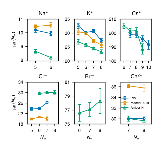
Figure 3: Effective Sternheimer factors for different quadrupolar ions at infinite dilution as a function of the number of water molecules $N_{\rm w}$ in the first hydration shell. We compare $\gamma_{\rm eff}$ obtained with the charge distribution in the PIM (blue circles), the Madrid-2019 model (yellow squares), and Amber14 FF parameters for the SPC/E water and ions (green triangles).

We now assess the quality of the Sternheimer approximation

$$V_{\alpha\beta}^{\rm SA}=(1+\gamma_{\rm eff})V_{\alpha\beta}^{\rm ext}$$ (14)

by considering the average prediction error for the squared EFG:

$$\sigma(\mathbf{V}^{2})=\frac{1}{M}\sum_{i=1}^{M}\left|\frac{\left(\mathbf{V}^{\rm SA}_{i}\right)^{2}-\left(\mathbf{V}^{\rm AI}_{i}\right)^{2}}{\left(\mathbf{V}^{\rm AI}_{i}\right)^{2}}\right|,$$ (15)

where $M=1000$ is the total number of configurations used for analysis, and $\mathbf{V}_{i}^{2}$ above stands for $\mathbf{V}_{i}:\mathbf{V}_{i}$ as computed from the Sternheimer approximation (14), $\left(\mathbf{V}^{\rm SA}_{i}\right)^{2}$, or from DFT GIPAW calculations, $\left(\mathbf{V}^{\rm AI}_{i}\right)^{2}$, for the same $i$-th configuration. The values of $\sigma(\mathbf{V}^{2})$ are listed in Tab. 1. Generally, for every ion and classical FF, we find $\sigma(\mathbf{V}^{2})$ to be quite large, indicating a 20-50% percent difference between $\left(\mathbf{V}^{\rm SA}\right)^{2}$ and $\left(\mathbf{V}^{\rm AI}\right)^{2}$ on average. Since such relatively large prediction error might considerably impact the resulting NMR relaxation rates that are directly proportional to the EFG variance $\left\langle\mathbf{V}^{2}\right\rangle$, in what follows we attempt to construct a better approximation for the EFG beyond the linear regime (14).

3.2 Effect of the first solvation shell

Since the main contribution to the EFG at the ion position arises from the closest solvent molecules⁴⁷, we start with investigating the potential impact of the hydration shell structure on the obtained effective Sternheimer factors. Fig. 3 shows $\gamma_{\rm eff}$ in the three considered classical FFs as a function of the number of water molecules $N_{\rm w}$ in the first hydration shell of an ion for Na⁺, K⁺, Cl^-, Br^-, and Ca²⁺ (see also Supporting Tab. S2). The first minimum of the ion-oxygen radial distribution function (RDF) was used as a boundary of the first solvation shell (see Supporting Fig. S6 and Supporting Tab. S1). As Li⁺ and Mg²⁺ feature a quite stable hydration shell structure (Supporting Fig. S7) with $N_{\rm w}=4$ and 6, respectively, they were excluded from the present analysis. Among the 1000 configurations used for the AI EFG parametrization, for a given ion and FF we selected only those that had at least 50 occurrences for a specific value of $N_{\rm w}$. The corresponding standard errors in Fig. 3 and Supporting Tab. S2 were also estimated using bootstrapping.

For most of the cations, $\gamma_{\rm eff}$ decreases with $N_{\rm w}$, yet enhanced statistics is necessary to decisively confirm this trend. Relatively small differences in $\gamma_{\rm eff}(N_{\rm w})$ (up to around 5%) are found for the Na⁺ and Ca²⁺ cations when comparing their two most probable coordination numbers (5 and 6 for Na⁺; 7 and 8 for Ca²⁺). The K⁺ cation has a quite broad distribution of coordination numbers (Supporting Fig. S7) and its $\gamma_{\rm eff}(N_{\rm w})$ features the most pronounced dependence on $N_{\rm w}$ among the ions considered. In particular, consistently across the three FFs, $\gamma_{\rm eff}$ for K⁺ decreases by up to $\approx 15$% when going from 5 to 8 water molecules in the first solvation shell. An up to 10% reduction in $\gamma_{\rm eff}$ is found for Cs⁺ for increasing $N_{\rm w}$ in the PIM and the Amber14 FF. For Cl^-, $\gamma_{\rm eff}$ increases by around 10% for increasing $N_{\rm w}$ from 5 to 7 in the PIM. For anions in the Amber14 FF, relatively small changes in the Sternheimer factor are seen with increasing $N_{\rm w}$, yet $\gamma_{\rm eff}$ tends to grow for Br^- and Cl^-. In summary, taking into account the hydration shell structure around an ion might be necessary to improve the prediction for the final relaxation rate (especially, in such cases as K⁺ and Cs⁺ for which $\gamma_{\rm eff}$ features a relatively pronounced dependence on $N_{\rm w}$).

3.3 Beyond the standard Sternheimer approximation

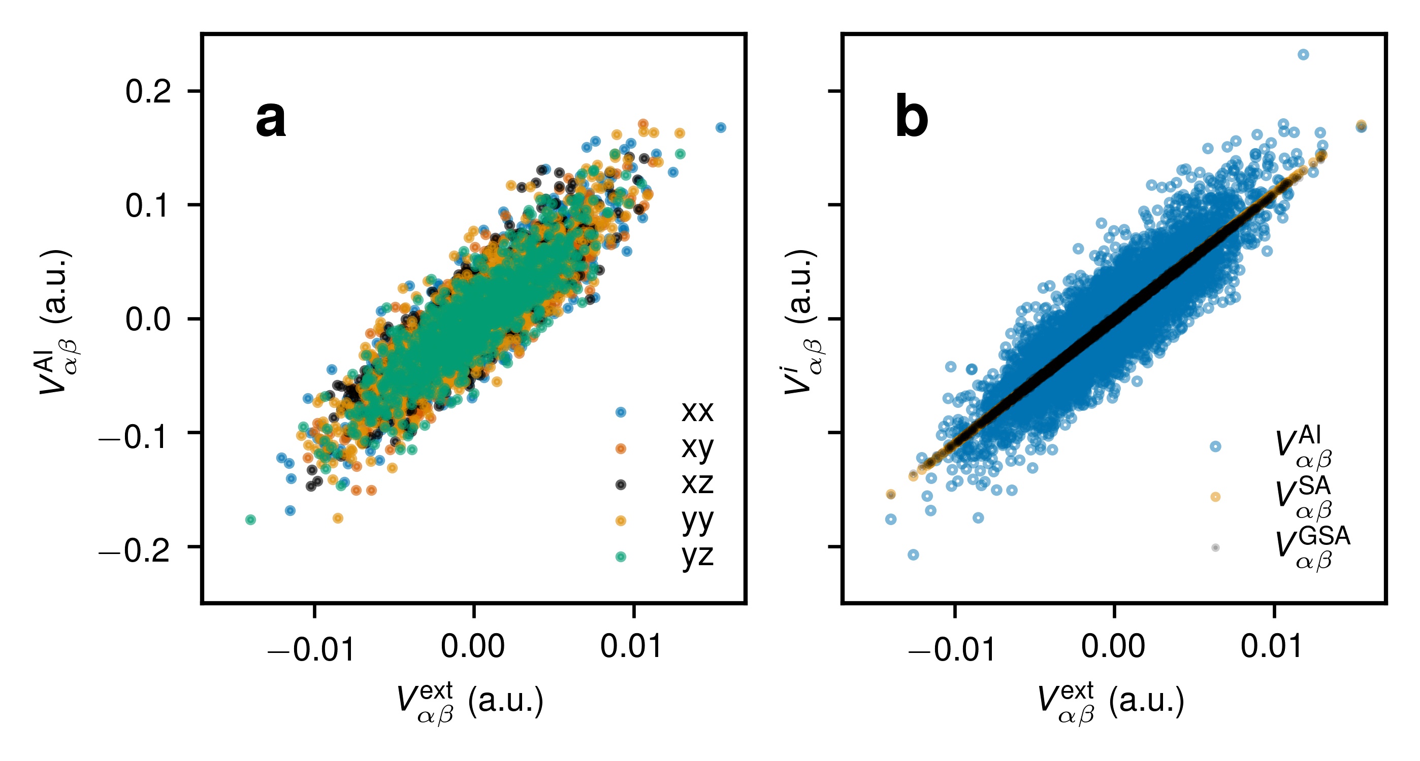
Figure 4: (a) Distribution of individual components of $V_{\alpha\beta}^{\rm AI}$ plotted versus $V_{\alpha\beta}^{\rm ext}$. (b), The original distribution of $V_{\alpha\beta}^{\rm AI}$ as a function of $V_{\alpha\beta}^{\rm ext}$ is compared to $V_{\alpha\beta}^{\rm SA}$ obtained using the linear Sternheimer approximation (14) and its generalized form (16). The EFGs shown here correspond to the Na⁺ ion in the PIM. Qualitatively similar dependencies are found for other ions and FFs.

To improve the quality of the original Sternheimer approximation (14) and to capture the differences in $\gamma_{\rm eff}$ generated by a distinct number of water molecules in the first solvation shell, we have attempted to construct a generalized linear Sternheimer approximation (GSA) that introduces couplings between diagonal and off-diagonal components of $V_{\alpha\beta}^{\rm ext}$. Although the scatter plots of $V^{\rm AI}_{\alpha\beta}$ plotted versus $V^{\rm ext}_{\alpha\beta}$ are practically identical for both diagonal and off-diagonal components (see Fig. 4a), yielding very similar component-wise Sternheimer factors, such GSA might be useful for capturing the differences in the electronic environments of an ion for each specific $N_{\rm w}$. Specifically, to parametrize the GSA we fit $V^{\rm AI}_{\alpha\beta}$ against $V_{\alpha\beta}^{\rm ext}$ employing the following expression:

$$V^{\rm GSA}_{\alpha\beta}=(1+\gamma_{1})V_{\alpha\beta}^{\rm ext}+\gamma_{2}\Gamma_{\alpha\gamma}V_{\gamma\delta}^{\rm ext}\Gamma^{T}_{\delta\beta},$$ (16)

where $\gamma_{1}$ and $\gamma_{2}$ are two Sternheimer-like factors, and $\Gamma_{\rm\alpha\beta}$ is an orthonormal matrix that generates an additional coupling between the components of $V_{\alpha\beta}^{\rm ext}$ and satisfies $\Gamma_{\alpha\gamma}\Gamma^{T}_{\gamma\beta}=\delta_{\alpha\beta}$. Note that by construction the term $\Gamma_{\alpha\gamma}V_{\gamma\delta}^{\rm ext}\Gamma^{T}_{\delta\beta}$ is traceless and symmetric. To perform the fit (16), we expressed $\Gamma_{\alpha\beta}$ using the Rodriguez formula:

$$\Gamma_{\alpha\beta}(\mathbf{\hat{e}},\psi)=(\cos\psi)\,\delta_{\alpha\beta}+(1-\cos\psi)\,\hat{e}_{\alpha}\hat{e}_{\beta}-(\sin\psi)\,\epsilon_{\alpha\beta\gamma}\hat{e}_{\gamma},$$ (17)

where $\epsilon_{\alpha\beta\gamma}$ is the Levi-Civita symbol and $\mathbf{\hat{e}}=(\sin\theta\cos\phi,\sin\theta\sin\phi,\cos\theta)^{T}$ is a unit vector. Thus, the angles $\psi,\theta,\phi$ and the two constants $\gamma_{1},\gamma_{2}$ are the fit parameters for the model (16). To assess the fit quality, in Fig. 4b we show $V_{\alpha\beta}^{\rm AI}$, $V_{\alpha\beta}^{\rm SA}$, and $V_{\alpha\beta}^{\rm GSA}$ plotted versus $V_{\alpha\beta}^{\rm ext}$ for the Na⁺ ion in the PIM (qualitatively similar results are obtained for other ions in all FFs considered). It is evident that the main error in $V_{\alpha\beta}^{\rm SA}$ comes from the failure of the simple linear approximation (14) to capture large off-diagonal deviations of $V^{\rm AI}_{\alpha\beta}$ when compared to $V^{\rm ext}_{\alpha\beta}$. Despite a more advanced structure of the GSA (16) with 4 additional fit parameters, $V_{\alpha\beta}^{\rm GSA}$ does not bring a considerable improvement to the resulting EFG variance (generally, a few percent reduction in $\sigma(\mathbf{V}^{2})$) and, similarly to $V_{\alpha\beta}^{\rm SA}$, it fails to capture significant off-diagonal deviations. In addition, we find that $\gamma_{1}$ in the fit (16) is quite close to $\gamma_{\rm eff}$ in (14), thus making the contribution of $\gamma_{2}\Gamma_{\alpha\gamma}V_{\gamma\delta}^{\rm ext}\Gamma^{T}_{\delta\beta}$ generally small.

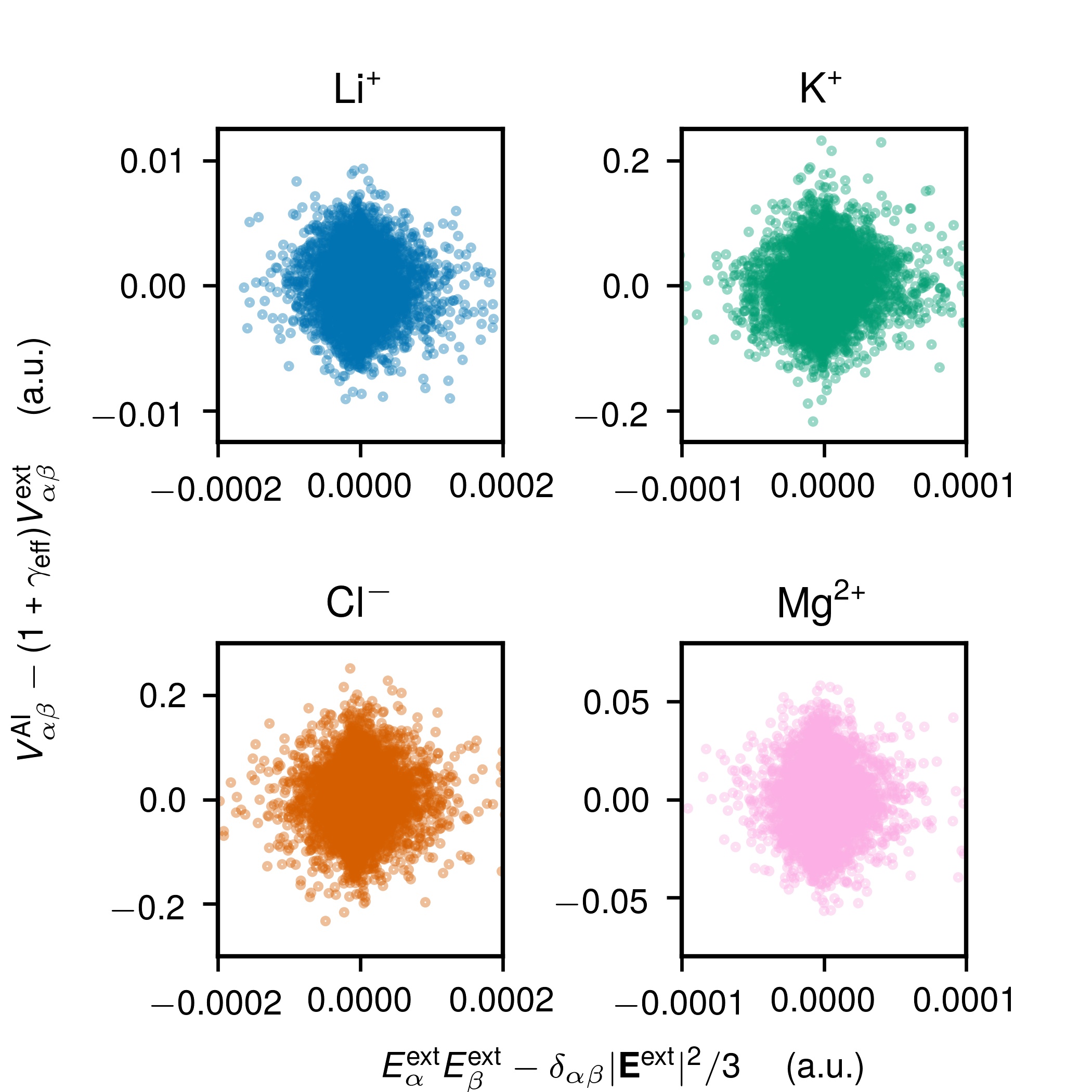
Figure 5: The difference between $V_{\alpha\beta}^{\rm AI}$ and $(1+\gamma_{\rm eff})V_{\alpha\beta}^{\rm ext}$ is plotted versus the traceless version of the tensor $E_{\alpha}^{\rm ext}E_{\beta}^{\rm ext}$ to account for non-linear effects (21) for different ions in the PIM. The absence of linear correlation is evident in all cases considered (also for other ions and FFs).

As the GSA (16) had not brought a considerable improvement in predicting the EFG variance compared to the AI data, we attempted to include the first-order non-linear correction to the EFG at the nucleus. In general, the EFG at the nucleus of an ion $V_{\alpha\beta}$ subject to external electric fields can be expressed as a perturbation series in the field and its gradients^{48, 49}:

$$V_{\alpha\beta}=V_{\alpha\beta}^{\rm ext}+g_{\alpha\beta,\gamma}E^{\rm ext}_{\gamma}+g_{\alpha\beta,\gamma\delta}V^{\rm ext}_{\gamma\delta}+\tfrac{1}{2}\epsilon_{\alpha\beta,\gamma\delta}E^{\rm ext}_{\gamma}E^{\rm ext}_{\delta}+\dots,$$ (18)

where the next order terms above correspond both to higher derivatives of the external field $E_{\alpha}^{\rm ext}$ and higher order non-linear terms. $g_{\alpha\beta,\gamma}$, $g_{\alpha\beta,\gamma\delta}$, and $\epsilon_{\alpha\beta,\gamma\delta}$ are tensorial susceptibilities that describe the response of the electronic cloud in different environments. In the case of an initially spherical electronic cloud of an ion, $g_{\alpha\beta,\gamma}=0$, whereas $g_{\alpha\beta,\gamma\delta}$ and $\epsilon_{\alpha\beta,\gamma\delta}$ both feature only one independent component, $\gamma$ and $\epsilon$, respectively^{49, 50}:

$$g_{\alpha\beta,\gamma\delta}=\gamma\left\{\frac{1}{2}\left(\delta_{\alpha\gamma}\delta_{\beta\delta}+\delta_{\alpha\delta}\delta_{\beta\gamma}\right)-\frac{1}{3}\delta_{\alpha\beta}\delta_{\gamma\delta}\right\}$$ (19)

$$\epsilon_{\alpha\beta,\gamma\delta}=\epsilon\left\{\frac{3}{4}\left(\delta_{\alpha\gamma}\delta_{\beta\delta}+\delta_{\alpha\delta}\delta_{\beta\gamma}\right)-\frac{1}{2}\delta_{\alpha\beta}\delta_{\gamma\delta}\right\}$$ (20)

Given the relations in Eqs. (19), (20) and assuming that the trace of $V_{\alpha\beta}^{\rm ext}$ is identically zero, the EFG in Eq. (18) simplifies to

$$V_{\alpha\beta}=(1+\gamma)V_{\alpha\beta}^{\rm ext}+\frac{3\epsilon}{4}\left(E_{\alpha}^{\rm ext}E_{\beta}^{\rm ext}-\frac{1}{3}\delta_{\alpha\beta}|\mathbf{E}^{\rm ext}|^{2}\right)+\dots,$$ (21)

where the first term in the equation above corresponds to the usual Sternheimer approximation and the second one conveys the first order non-linear correction with the hyperpolarizability $\epsilon$. In Fig. 5, we plot the difference between $V^{\rm AI}_{\alpha\beta}$ and $(1+\gamma_{\rm eff})V^{\rm ext}_{\alpha\beta}$ versus the traceless tensor ${\widetilde{E}}_{\alpha\beta}^{\rm ext}=E_{\alpha}^{\rm ext}E_{\beta}^{\rm ext}-\delta_{\alpha\beta}|\mathbf{E}^{\rm ext}|^{2}/3$ for Li⁺, K⁺, Cl^-, and Mg²⁺ in the PIM (qualitatively similar results are found for other ions in all FFs considered). In agreement with earlier results on a smaller number of configurations⁵¹ and in contrast to crystalline atomic environments⁴⁹, the overall symmetric scatter plots centered at the origin indicate the absence of significant linear correlation between $V^{\rm AI}_{\alpha\beta}-(1+\gamma_{\rm eff})V^{\rm ext}_{\alpha\beta}$ and ${\widetilde{E}}_{\alpha\beta}^{\rm ext}$. The fact that the latter two quantities are uncorrelated in the present liquid state system might be related to different symmetry properties of the $V_{\alpha\beta}$ and ${\widetilde{E}}_{\alpha\beta}$ tensors. For instance, for certain configurations that feature a symmetry axis the electric field can be vanishing at the origin corresponding to the nucleus position, whereas the EFG can still remain non-zero. In addition, we attempted to correlate $V^{\rm AI}_{\alpha\beta}-(1+\gamma_{\rm eff})V^{\rm ext}_{\alpha\beta}$ with other higher order non-linear terms like $(\mathbf{E}^{\rm ext})^{2}V_{\alpha\beta}$, $(\mathbf{V}^{\rm ext})^{2}{\widetilde{E}}_{\alpha\beta}^{\rm ext}$, ${\widetilde{E}}_{\alpha\gamma}^{\rm ext}V_{\gamma\beta}$, however, similarly to Fig. 5, in all cases no pronounced correlation has been identified (not shown). Therefore, in the following we use the initial Sternheimer approximation for the prediction of NMR relaxation rates.

4 NMR relaxation rates

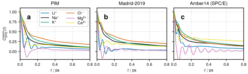
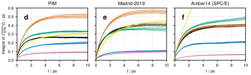
Figure 6: Autocorrelation function of the the electric field gradient at the ion position in different classical FFs: normalized EFG ACF and its running integral in the PIM ((a) and (d)), the Madrid-2019 model ((b) and (e)), and Amber14 FF parameters for the SPC/E water and ions ((c) and (f)) for K⁺, Na⁺, Li⁺, Cl^-, and Mg²⁺. The legend shown in (a) also applies to all panels; panels (a), (b) and (c) share the same range on both axes, and so do panels (d), (e) and (f). Shaded regions around a curve correspond to the standard error obtained from independent simulation runs.

We finally consider the EFG ACFs from different classical FFs and the resulting NMR relaxation rates. Figs. 6a–c feature the normalized ACFs of $V^{\rm ext}_{\alpha\beta}$, $C_{\rm EFG}^{\rm norm}(t)$, for Li⁺, Na⁺, K⁺, Cl^-, Mg²⁺ and Ca²⁺ in the PIM, Madrid-2019 model, and the Amber14 FF parameters for the SPC/E water and ions. Additional results for larger and more polarizable solutes such as Cs⁺, Br^-, and I^- as well as a comparison between the EFG ACFs for the alkali metals are available in the Supporting Fig. S1. Interestingly, the structure of the EFG ACFs remains similar across the distinct FFs considered and is consistent with previous studies ^{2, 7, 8, 9, 10, 47, 52}. In general, $C_{\rm EFG}^{\rm norm}(t)$ relaxes in two steps with a pronounced short-range oscillatory regime for the smaller Li⁺ and Mg²⁺ ions, associated with their tight confinement in the solvation shell ⁴⁷. Furthermore, the ACF for Li⁺ is positive at all times in the PIM and Amber14 FF, whereas in the Madrid-2019 model it shows a negative region at around 0.1 ps. In addition, a less pronounced oscillatory regime of $C_{\rm EFG}^{\rm norm}(t)$ at short times is observed for the Ca²⁺ ion as well. In the Amber14 FF, as compared to the two other models, the EFG ACF of Mg²⁺ shows much more striking oscillations, whereas the decay for Ca²⁺ is considerably slower. This again illustrates the difficulty for non-polarizable models with formal ionic charges to accurately model multivalent ionic species^{53, 54}. For larger ions, $C_{\rm EFG}^{\rm norm}(t)$ develops two clear relaxation steps. Interestingly, and consistently with AIMD simulations⁵, $C_{\rm EFG}^{\rm norm}(t)$ develops a “notch” at very short times for the anions and for Cs⁺, a feature associated with the librational motion of water molecules in the hydrogen bond network⁵. Finally, the reasonable agreement between $C_{\rm EFG}^{\rm norm}(t)$ obtained here and in AIMD^{3, 5} confirms that the short time stretching and bending vibrational modes of water molecules (neglected in the rigid water models employed here) do not play a significant role in the form of the EFG relaxation.

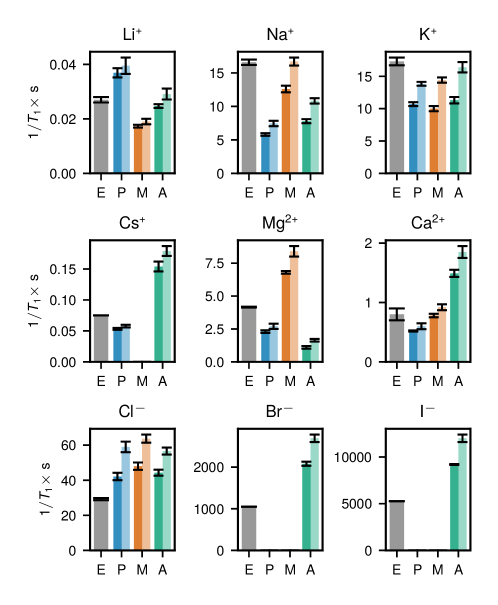
Figure 7: Predicted NMR relaxation rates of quadrupolar nuclei at infinite dilution. For every ion, we indicate an experimental value (E), as well as the rate obtained using the PIM (P), the Madrid-2019 model (M), and Amber14 FF parameters for the SPC/E water and ions (A). For the P, M and E cases, the two adjacent columns indicate the $1/T_{1}$ value obtained using the EFG variance from the Sternheimer approximation $\langle\mathbf{V}_{\rm SA}^{2}\rangle$ (left dark-colored columns) and directly from AI DFT calculations $\langle\mathbf{V}_{\rm AI}^{2}\rangle$ (right light-colored columns).

As we show with running integrals of $C_{\rm EFG}^{\rm norm}(t)$ in Figs. 6d–f and Supporting Fig. S1, accurate ACFs over around 10 ps (and even more in some cases) are required to precisely measure the effective EFG correlation time $\tau_{c}$ (4). All parameters of the EFG relaxation, in particular $\langle\mathbf{V}_{\rm ext}^{2}\rangle$ and $\tau_{c}$, for all ions and FFs considered are again summarized in the Supporting Tab. S3. Small differences in $\tau_{c}$ are found across the three FFs considered, yet in most cases $\tau_{c}$ does not exceed 0.5 ps. For Ca²⁺ in the Amber14 FF, $\tau_{c}=1.06$ ps, likely being an overestimation in comparison to the two other FFs ($\tau_{c}=0.31$ ps in the PIM and 0.44 ps in the Madrid-2019 for Ca²⁺, see also Supporting Fig. S3).

The variance of the external EFG $\langle\mathbf{V}_{\rm ext}^{2}\rangle$ decreases horizontally along the periodic table, reflecting its dependence on the ionic size. Additionally, we list in the Supporting Tab. S3 the EFG variance $\langle\mathbf{V}_{\rm SA}^{2}\rangle$ obtained with the Sternheimer approximation (14) using $\gamma_{\rm eff}$ from Tab. 1 as well as the variance $\langle\mathbf{V}_{\rm AI}^{2}\rangle$ obtained directly from the AI EFGs on our sets of 1000 configurations for each ion. It is evident from this comparison that the failure of the Sternheimer approximation in capturing the dispersion of the AI EFG (Fig. 4b) always results in $\langle\mathbf{V}_{\rm SA}^{2}\rangle$ being smaller than $\langle\mathbf{V}_{\rm AI}^{2}\rangle$. In some cases, as shown further below, the use of $\langle\mathbf{V}_{\rm AI}^{2}\rangle$ instead of $\langle\mathbf{V}_{\rm SA}^{2}\rangle\equiv(1+\gamma_{\rm eff})^{2}\langle\mathbf{V}_{\rm ext}^{2}\rangle$ in Eq. (3) yields a better prediction for the final NMR relaxation rates. Nevertheless, a direct replacement of $\langle\mathbf{V}_{\rm SA}^{2}\rangle$ by $\langle\mathbf{V}_{\rm AI}^{2}\rangle$ in Eq. (3) does not entirely account for the errors introduced by the Sternheimer approximation (see discussion in the SI). Consistently across the three FFs, a 25–35% difference between $\langle\mathbf{V}_{\rm AI}^{2}\rangle$ and $\langle\mathbf{V}_{\rm SA}^{2}\rangle$ is found for the Na⁺, K⁺, and Cl^-, potentially leading to a marked impact on the final relaxation rate. In addition, a somewhat better correspondence between $\langle\mathbf{V}_{\rm SA}^{2}\rangle$ and $\langle\mathbf{V}_{\rm AI}^{2}\rangle$ can be achieved if a direct fit between the squared EFGs $\mathbf{V}_{\rm AI}^{2}\simeq(1+\gamma^{\prime}_{\rm eff})^{2}\mathbf{V}_{\rm ext}^{2}$ for $\gamma_{\rm eff}^{\prime}$ is performed, generally resulting in larger values of $\gamma^{\prime}_{\rm eff}$ as compared to $\gamma_{\rm eff}$ in Tab. 1. However, such a fit simultaneously yields bigger $\sigma(\mathbf{V}^{2})$ and similarly fails to capture the dispersion of the AI EFGs (not shown). Finally, the differences in $\langle\mathbf{V}_{\rm ext}^{2}\rangle$ and consequently in $\langle\mathbf{V}_{\rm SA}^{2}\rangle$ and $\langle\mathbf{V}_{\rm AI}^{2}\rangle$ again highlight the importance of the charge and density distributions around an ion on the resulting EFG at the ion position.

Finally, it is instructive to compare the EFG relaxation parameters obtained here with classical MD with that from the AIMD studies^{6, 3, 5}. In Ref. 3, $\tau_{c}=0.26(0.06)$ ps and $\langle\mathbf{V}^{2}\rangle=0.21(0.01)$ (in a.u.) for ³⁵Cl^-. In our case, for the same anion we find $\tau_{c}=0.51(0.02)$ ps and $\langle\mathbf{V}_{\rm SA}^{2}\rangle=0.087(0.002)$ in the PIM; $\tau_{c}=0.56(0.02)$ ps and $\langle\mathbf{V}_{\rm SA}^{2}\rangle=0.089(0.002)$ in the Madrid-2019 model; $\tau_{c}=0.40(0.01)$ ps and $\langle\mathbf{V}_{\rm SA}^{2}\rangle=0.115(0.002)$ in the Amber14 FF. Similarly for ²³Na⁺, Ref. 3 indicates $\tau_{c}=0.13(0.03)$ ps and $\langle\mathbf{V}^{2}\rangle=0.028(0.001)$ (in a.u.), whereas in our case we obtain we find $\tau_{c}=0.26(0.01)$ ps and $\langle\mathbf{V}_{\rm SA}^{2}\rangle=0.014(0.003)$ in the PIM; $\tau_{c}=0.41(0.01)$ ps and $\langle\mathbf{V}_{\rm SA}^{2}\rangle=0.0197(0.0004)$ in the Madrid-2019 model; $\tau_{c}=0.41(0.01)$ ps and $\langle\mathbf{V}_{\rm SA}^{2}\rangle=0.0122(0.0002)$ in the Amber14 FF. The AIMD results provide somewhat smaller estimates for $\tau_{c}$ when compared to classical MD, yet enhanced values of the EFG variance. As shown below, classical MD can also yield quite good values for the NMR relaxation rates, provided that $\gamma_{\rm eff}$, $\langle\mathbf{V}_{\rm ext}^{2}\rangle$, and $\tau_{c}$ are obtained consistently for a FF at hand.

Table 2: Comparison between the NMR relaxation rates from experiments and classical MD simulations with various FFs for a series of quadrupolar ions at infinite dilution.

Ion	$I$	$Q$ (mb)	$1/T_{1}$ (s-1)
			Experiment	PIM	Madrid-2019	Amber14
7Li+	3/2	-40.1	0.02756, 11	0.037(0.002)	0.0173(0.0005)	0.0247(0.0007)
39K+	3/2	+60.3	16.757, 17.858	10.7(0.3)	10.0(0.4)	11.3(0.5)
23Na+	3/2	+104	17.057, 16.256	5.8(0.2)	12.6(0.5)	7.8(0.3)
133Cs+	7/2	-3.43	0.07513, 58	0.053(0.002)	—	0.154(0.008)
35Cl-	3/2	-81.12	29.2(0.6)59, 2858	42.1(2.1)	48.0(2.1)	44.3(1.7)
81Br-	3/2	257.9	105013, 58	—	—	2080(50)
127I-	5/2	-688.22	527013, 460058	—	—	9200(300)
25Mg2+	5/2	+199.4	4.16(0.03)59	2.3(0.1)	6.8(0.1)	1.1(0.1)
43Ca2+	7/2	-40.8	0.8(0.1)60	0.52(0.01)	0.78(0.03)	1.49(0.06)

The final NMR relaxation rates $1/T_{1}$ for different ions obtained with the three classical FFs considered here are shown in Fig. 7 and also summarized in Tab. 2, together with the corresponding experimental values. For ⁷Li⁺, we find a quite good prediction for $1/T_{1}$ with the largest relative error $\left|1-T_{1}^{\rm exp}/T_{1}^{\rm sim}\right|$ of around 35% in both the PIM and the Madrid-2019 model when compared to the experimental value of 0.027 s^-1 that is measured for ⁷Li⁺ in D₂O (which corresponds to the quadrupolar contribution only). The value of 0.0247(0.0007) for ⁷Li⁺ in the Amber14 FF is in very good agreement with the experimental value. Recently, the latter model has been used to determine the concentration dependence of the quadrupolar contribution to the rate of ⁷Li⁺ in simulations, yet a value of $\gamma_{\infty}=0.17$ was used to account for the electronic cloud polarization effects and ultimately resulted in some differences between the simulation and experimental results at lower concentrations ¹¹. Here we show that this discrepancy can be overcome by considering the model specific Sternheimer factor $\gamma_{\rm eff}$.

For ²³Na⁺, the Madrid-2019 model provides the best estimate for $1/T_{1}$ that is around 20% smaller than the experimental value. For ³⁹K⁺, all FFs considered yield quite close quadrupolar relaxation rates, being approximately 40% smaller than the experimental value. On the other hand, for the ³⁵Cl^- anion, the rates from all three FFs are also quite close to each other but 40–60% larger than those from the experiment. We find that the use of $\langle\mathbf{V}_{\rm AI}^{2}\rangle$ instead of $\langle\mathbf{V}_{\rm SA}^{2}\rangle$ improves the rate predictions for Na⁺ and K⁺, yet leads to larger discrepancies for Cl^- and the other two anions Br^- and I^-, the parameters for which are available in the Amber14 FF only. For the two divalent cations considered here, ²⁵Mg²⁺ and ⁴³Ca²⁺, we find that the PIM and the Madrid-2019 model provide better estimates for the relaxation rates. In particular, very good agreement for with the experimental rates is found ⁴³Ca²⁺ (35% error in the PIM and almost quantitative agreement in the Madrid-2019 model), whereas a much higher discrepancy is observed in the Amber14 FF. Somewhat larger errors are found for ²⁵Mg²⁺, however still better than in the Amber14 FF whose rate is around 4 times smaller than the experimental one. Finally, it is interesting to assess the rates obtained for larger and highly polarizable solutes like ¹³³Cs⁺, ⁸¹Br^-, and ¹²⁷I^-. The parameters for the latter three species are available in the Amber14 FF, and in each case $1/T_{1}$ from the simulations is about twice as high as the experimental one. On the contrary, for ¹³³Cs⁺ in the PIM, the resulting rate $1/T_{1}^{\rm PIM}=0.053(0.002)$ s^-1 is in reasonable agreement with the experimental one $1/T_{1}^{\rm exp}=0.075$ s^-1, and is somewhat better than the state-of-the-art AIMD value obtained from the EFGs with relativistic effects included ⁵ $1/T_{1}^{\rm AIMD}=0.033(0.006)$ s^-1. This illustrates that classical MD is also suitable for computing the NMR relaxation rates for divalent as well as large and strongly polarizable ionic species, provided that more sophisticated methods to account for the electronic polarizability are employed.

5 Discussion and concluding remarks

We have shown in this work that accurate NMR relaxation rates can be obtained from classical MD simulations, provided that local electron cloud polarization effects are taken into account consistently for each specific classical FF considered. We have employed a Sternheimer-like parametrization for the electron cloud contribution to the EFG at the ion position by comparing the classical $V_{\alpha\beta}^{\rm ext}$ and quantum $V_{\alpha\beta}^{\rm AI}$ EFGs on a set of classically generated configurations. We have found that a linear relationship between $V_{\alpha\beta}^{\rm AI}$ and $V_{\alpha\beta}^{\rm ext}$ holds well in all the cases considered (Fig. 1), allowing to define effective model-dependent Sternheimer factors $\gamma_{\rm eff}$ (Fig. 2). Yet, such Sternheimer factors show a quite pronounced dependence on the FFs at hand. For instance, the difference in $\gamma_{\rm eff}$ across the classical models considered here can be up to 50%, which is in some cases comparable to the difference between $\gamma_{\rm eff}$ and $\gamma_{\rm\infty}$ that was obtained for a more simplistic Watson sphere approximation. We have found that considerable variations in $\gamma_{\rm eff}$ are due to the changes in the charge density representation of the employed water model (that is, via the chosen set of point charges and dipoles), whereas further differences are likely caused by variations in the solvation shell structure. In summary, $\gamma_{\rm eff}$ might be reasonably transferable for electrolyte FFs that employ the same water model, whereas the transferability is likely limited across FFs with different water models.

The error in the predicted EFG variance using such an effective Sternheimer approximation (14) might be quite large (up to 50% for certain ions) when compared to the AI EFGs (Tab. 1). In particular, the linear Sternheimer-like approximations that relate $V_{\alpha\beta}^{\rm AI}$ and $V_{\alpha\beta}^{\rm ext}$ fail to capture the large dispersion in $V_{\alpha\beta}^{\rm AI}$ (Fig. 4). We have demonstrated that for the present liquid matter systems it is very challenging to systematically reduce the prediction error, for instance by taking into account non-linear effects (21) that were shown to be essential for highly symmetric crystalline environments⁴⁹. Some explanations can be proposed to rationalize this finding: $(i)$ in the present parametrization we employ $V_{\alpha\beta}^{\rm ext}$ generated by the external classical charge distribution around the given ion that can be very sensitive to the quality of the FF at hand – while some FFs can provide a better approximation for the ab initio charge density, it is still hard to systematically assess its impact as the partitioning between internal and external charges includes some degree of arbitrariness in condensed phase systems; $(ii)$ the local polarization effects that have a considerable impact on the EFG at the nucleus might be strongly dependent on the instantaneous hydration shell structure and solute-solvent interactions; $(iii)$ the inclusion of non-linear corrections to the EFG at the nucleus in liquid state systems can be limited by different symmetry properties of the $V_{\alpha\beta}$ and $E^{\rm ext}_{\alpha\beta}$ tensors. In summary, it might be possible to construct an improved EFG parametrization strategy by explicitly considering the local atomic environment around an ion, as this was done recently in the context of NMR for chemical shifts^{61, 62}. In particular, correlating local solvent structure with the variable of interest (in this case, the EFG tensor) using machine learning methods provides a possible direction to improve predictions from FF MD, as evidenced by recent progress in the field of vibrational spectroscopy ^{63, 64}. The quality of the classical FF used for simulating the electrolyte dynamics constitutes another important dimension of the problem. Here we have observed that the incorporation of electronic polarizability either through induced dipoles as in the PIM or through scaled ionic charges as it the Madrid-2019 model in many cases leads to better values of the NMR relaxation rates when compared to the non-polarizable Amber14 FF based on the SPC/E water and formal ionic charges. In particular, this is valid for the divalent Mg²⁺ and Ca²⁺ ions as well as for the large and highly polarizable Cs⁺ ion (Fig. 7). However, surprisingly, for smaller and less polarizable species, the non-polarizable Amber14 FF also provides quite good predictions for the final NMR relaxation rates. Furthermore, while the FFs used in this work employ rigid water molecules, the inclusion of stretching and bending modes in flexible water geometries might be necessary for a more accurate description of the EFG relaxation at short time scales in classical MD. Quantitatively, the $1/T_{1}$ predictions obtained here are comparable and in some cases superior to the AIMD results^{3, 5}. The fact that computationally more efficient non-polarizable and scaled charge models are suitable for determining the NMR relaxation rates with reasonable accuracy, provided that a model-specific Sternheimer factor parametrized on ab initio calculations is used, paves the way for exploring the microscopic origins of many NMR relaxation phenomena, in particular those involving the concentration and pressure dependence of $1/T_{1}$ in concentrated electrolyte solutions and its relation to collective symmetry-breaking fluctuations in the solvation shell⁵².

Associated content

The Supporting Information is available free of charge at http://pubs.acs.org.

Additional discussion on the errors introduced by the Sternheimer approximation (Section S1); EFG ACFs in an explicitly electroneutral system and sampled in the $NVE$ ensemble (Figure S1); additional EFG ACFs and Sternheimer parametrization for Cs⁺, Br^-, and I^- (Figure S2); comparison between the EFG ACFs and their integrals for Ca²⁺ in different FFs (Figure S3); the effect of swapping the charge density representation between the PIM and Madrid-2019 FFs on the resulting $\gamma_{\rm eff}$ (Figures S4 and S5); ion-oxygen RDFs (Figure S6); structure of the first solvation shell of ions in the three classical FFs considered (Figure S7); coordination numbers of the first solvation shell for all ions in the three classical FFs considered (Table S1); effective Sternheimer factors as a function of the number of water molecules in the first solvation shell in different FFs (Table S2); parameters of the EFG relaxation for all ions in the three classical FFs considered (Table S3).

Notes

The authors declare no competing financial interest.

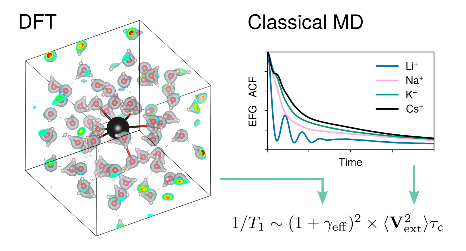
Figure 8: For Table of Contents Only.

Supporting Information

S1 Details on the Sternheimer approximation

In the present work, the system dynamics was generated using classical, force-field based molecular dynamics (FF MD). In principle, the most accurate way of calculating the quadrupolar NMR relaxation rates using FF MD would be by evaluating the ab initio (AI) electric field gradients (EFGs) ${\mathbf{V}}_{\rm AI}$ at the ion position on every system configuration of interest. The dynamics of ${\mathbf{V}}_{\rm AI}$ fluctuations is then given by the variance $\langle{\mathbf{V}}^{2}_{\rm AI}\rangle$ and the effective correlation time $\tau_{\rm c,\,AI}$:

$$\tau_{\rm c,\,AI}=\langle{\mathbf{V}}^{2}_{\rm AI}\rangle^{-1}\,\int_{0}^{\infty}{\rm d}t\,\langle{\mathbf{V}}_{\rm AI}(t)\,{:}{\mathbf{V}}_{\rm AI}(0)\rangle.$$ (22)

Note that the dynamics of AI EFGs computed on system configurations generated using ab initio molecular dynamics (AIMD) might somewhat differ from that with FF MD.

The calculation of AI EFGs ${\mathbf{V}}_{\rm AI}$ can be quite expensive if done for a large number of configurations. In practice, here we employed the Sternheimer approximation that relates the classical, external EFGs ${\mathbf{V}}_{\rm ext}$ computed with point charges and dipoles of a FF at hand to ${\mathbf{V}}_{\rm AI}$ via the effective Sternheimer factor $\gamma_{\rm eff}$:

$${\mathbf{V}}_{\rm AI}\simeq(1+\gamma_{\rm eff}){\mathbf{V}}_{\rm ext}$$ (23)

The dynamics of ${\mathbf{V}}_{\rm ext}$ fluctuations are characterized by the variance $\langle{\mathbf{V}}^{2}_{\rm ext}\rangle$ and the effective correlation time $\tau_{\rm c,\,ext}$ (simply denoted by $\tau_{\rm c}$ in the main text):

$$\tau_{\rm c,\,ext}=\langle{\mathbf{V}}^{2}_{\rm ext}\rangle^{-1}\,\int_{0}^{\infty}{\rm d}t\,\langle{\mathbf{V}}_{\rm ext}(t)\,{:}{\mathbf{V}}_{\rm ext}(0)\rangle.$$ (24)

Nevertheless, the Sternheimer approximation does not perfectly capture ${\mathbf{V}}_{\rm AI}$ (Fig. 4 of the main text), i.e. there exists an error term $\Delta{\mathbf{V}}$:

$${\mathbf{V}}_{\rm AI}(t)=(1+\gamma_{\rm eff}){\mathbf{V}}_{\rm ext}(t)+\Delta{\mathbf{V}}(t)$$ (25)

The ACF of AI EFG can thus be recast as follows:

$$\begin{split}\langle{\mathbf{V}}_{\rm AI}(t)\,{:}{\mathbf{V}}_{\rm AI}(0)\rangle&=(1+\gamma_{\rm eff})^{2}\langle{\mathbf{V}}_{\rm ext}(t)\,{:}{\mathbf{V}}_{\rm ext}(0)\rangle+\langle\Delta{\mathbf{V}}(t)\,{:}\Delta{\mathbf{V}}(0)\rangle\\ &+2(1+\gamma_{\rm eff})\langle{\mathbf{V}}_{\rm ext}(t)\,{:}\Delta{\mathbf{V}}(0)\rangle.\end{split}$$ (26)

Finally, by integrating Eq. (26) over time, we find

$$\begin{split}\langle{\mathbf{V}}^{2}_{\rm AI}\rangle\,\tau_{\rm c,\,AI}&=(1+\gamma_{\rm eff})^{2}\langle{\mathbf{V}}^{2}_{\rm ext}\rangle\,\tau_{\rm c,\,ext}+\langle\Delta{\mathbf{V}}^{2}\rangle\,\tau_{\rm c,\,\Delta}+2(1+\gamma_{\rm eff})\int_{0}^{\infty}{\rm d}t\,\langle{\mathbf{V}}_{\rm ext}(t)\,{:}\Delta{\mathbf{V}}(0)\rangle,\end{split}$$ (27)

where $\langle\Delta{\mathbf{V}}^{2}\rangle$ is the variance of the error term $\Delta{\mathbf{V}}$ and $\tau_{\rm c,\,\Delta}$ is its effective correlation time

$$\tau_{\rm c,\,\Delta}=\langle{\Delta\mathbf{V}}^{2}\rangle^{-1}\,\int_{0}^{\infty}{\rm d}t\,\langle{\Delta\mathbf{V}}(t)\,{:}{\Delta\mathbf{V}}(0)\rangle.$$ (28)

Evidently from Eq. (27), both the variance of $\langle{\mathbf{V}}^{2}_{\rm AI}\rangle$ and the correlation time of the AI EFG $\tau_{\rm c,\,AI}$ are affected by the fluctuations of the error term $\Delta\mathbf{V}$.

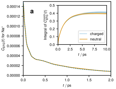
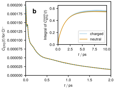
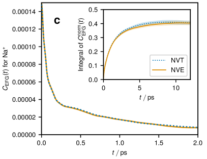
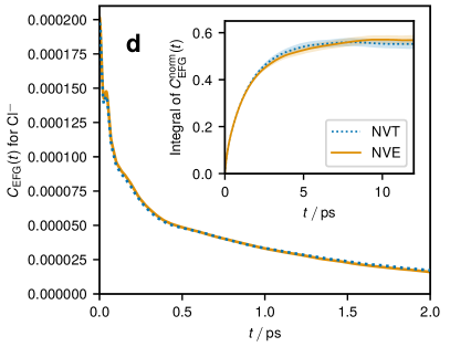
Figure S1: Simulation details. Comparison between the EFG ACF and the integral of the normalized EFG ACF (inset) for Na⁺ (a) and Cl^- (b) as simulated in a smaller non-electroneutral system (blue dashed lines) with $N=256$ water molecules and 1 ion and a larger electroneutral system (solid yellow lines) with $N=1000$ water molecules and 1 NaCl ion pair. For the smaller systems, 5 independent simulation runs of length 1 ns were performed. For the larger system, the results were extracted from 1 run of length 10 ns. Comparison between the EFG ACF and the integral of the normalized EFG ACF (inset) for Na⁺ (c) and Cl^- (d) as sampled in the $NVT$ (blue dashed lines) and $NVE$ (solid yellow lines) ensemble. The $NVT$ runs correspond to the smaller system in a and b. The $NVE$ runs were performed in a single 5 ns simulation for the system with $N=256$ water molecules using an equilibrated system state form $NVT$ simulation as a starting configuration. In all cases, the ions and water were simulated using the Madrid-2019 model.

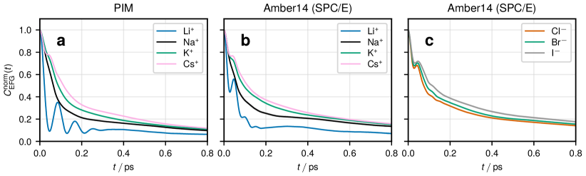
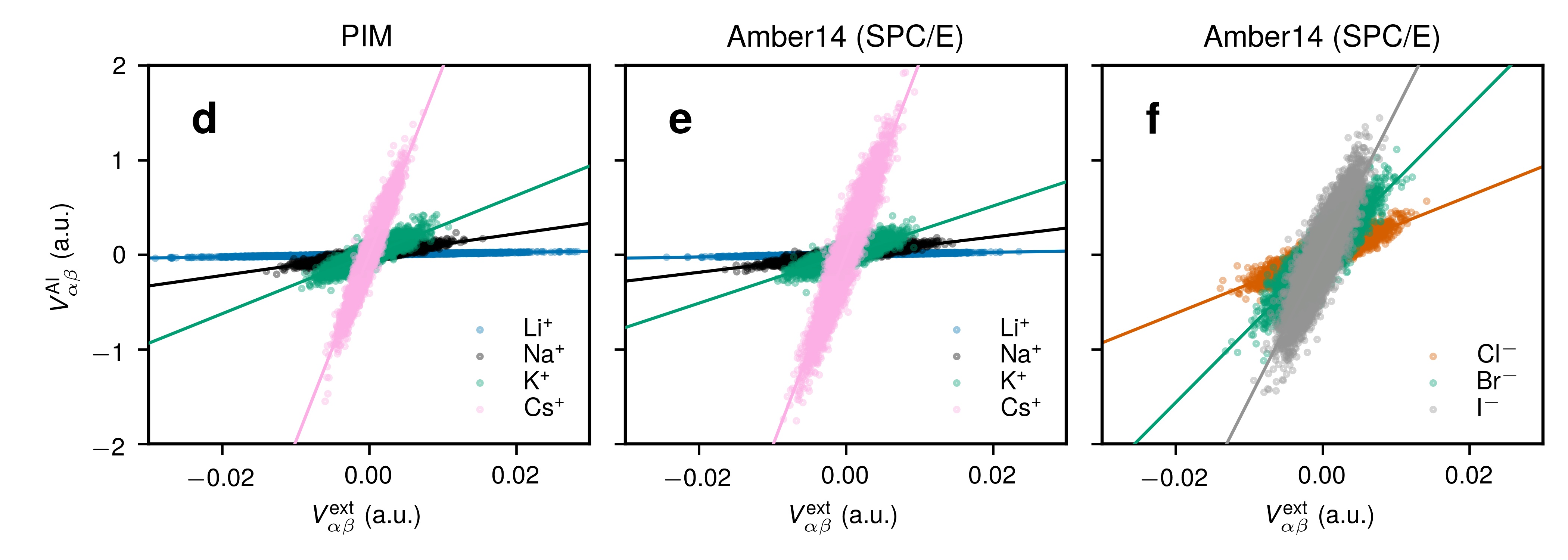
Figure S2: Normalized EFG ACFs for alkali metal ((a) in the PIM and (b) in the Amber14 FF) and halide ions ((c) in the Amber14 FF). The corresponding validation of the Sternheimer approximation for the systems in (a), (b), and (c) is shown in (d), (e), and (f), respectively.

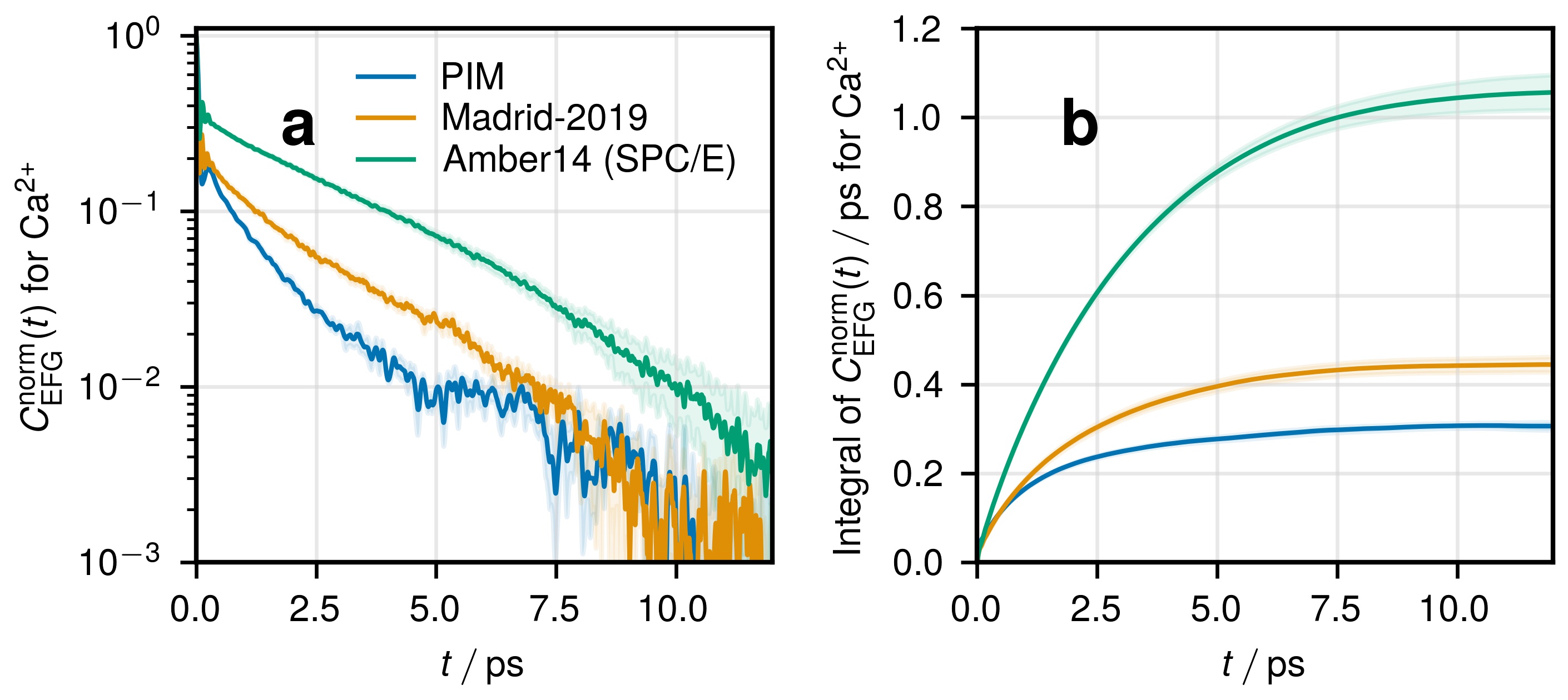
Figure S3: Comparison between the normalized EFG ACFs (a) and their integrals (b) for Ca²⁺ in the PIM (blue lines), Madrid-2019 model (yellow lines), and the Amber14 FF (green lines). (a) and (b) share the same legend shown in (a).

Table S1: Structure of the first hydration shell in different classical FFs. The first minimum of $g_{{\rm ion-O}}(r)$, $r_{1,{\rm min}}$, is used to estimate the first shell coordination number $CN_{1}=4\pi\rho_{\rm O}\int_{0}^{r_{1,{\rm min}}}{\rm d}r\,r^{2}g_{{\rm ion-O}}(r)$ with $\rho_{\rm O}$ the number density of oxygen atoms in the simulation box.

Ion	$r^{\rm PIM}_{1,{\rm min}}$ (Å)	$CN^{\rm PIM}_{1}$	$r^{\rm Madrid-2019}_{1,{\rm min}}$ (Å)	$CN^{\rm Madrid-2019}_{1}$	$r^{\rm Amber14}_{1,{\rm min}}$ (Å)	$CN^{\rm Amber14}_{1}$
Li+	2.68	4.0	2.69	4.0	2.67	4.2
Na+	3.28	5.8	3.15	5.5	3.17	5.8
K+	3.63	6.8	3.53	6.8	3.53	7.0
Cs+	4.12	8.9	—	—	3.82	7.8
Mg2+	2.96	6.0	3.00	6.0	2.88	6.0
Ca2+	3.53	7.4	3.24	7.3	3.22	8.0
Cl-	3.82	6.2	3.68	5.9	3.80	6.9
Br-	—	—	—	—	3.94	7.0
I-	—	—	—	—	4.15	7.3

Table S2: Effective Sternheimer factors as a function of the number of water molecules $N_{\rm w}$ in the first solvation shell as obtained for different classical FFs. The values in the parentheses indicate the standard error obtained using bootstrapping.

Ion	$\gamma^{\rm PIM}_{\rm eff}(N_{\rm w})$	$\gamma^{\rm Madrid-2019}_{\rm eff}(N_{\rm w})$	$\gamma^{\rm Amber14\,(SPC/E)}_{\rm eff}(N_{\rm w})$
Na+	5: 10.19(0.19) 6: 9.94(0.14)	5: 10.46(0.12) 6: 10.55(0.20)	5: 8.65(0.14) 6: 8.18(0.11)
K+	5: 32.60(0.91) 6: 30.20(0.48) 7: 30.67(0.56) 8: 27.31(0.79)	5: 30.44(1.00) 6: 29.98(0.50) 7: 27.21(0.54) 8: 25.75(0.98)	5: 26.88(0.85) 6: 25.73(0.49) 7: 24.41(0.45) 8: 23.30(0.70)
Cs+	7: 199.0(2.0) 8: 198.6(2.0) 9: 195.9(2.2) 10: 191.7(3.3)	—	6: 205.2(1.9) 7: 201.5(1.8) 8: 201.7(2.2) 9: 188.6(3.7)
Cl-	5: 23.75(0.50) 6: 23.92(0.37) 7: 26.18(0.48)	5: 19.91(0.38) 6: 20.69(0.30) 7: 20.09(0.64)	6: 29.69(0.43) 7: 30.03(0.40) 8: 30.11(0.69)
Br-	—	—	6: 76.6(1.2) 7: 77.1(1.0) 8: 78.3(1.8)
I-	—	—	6: 154.5(2.4) 7: 149.4(2.2) 8: 152.5(3.0)
Ca2+	7: 30.02(0.16) 8: 30.07(0.29)	7: 36.18(0.33) 8: 35.77(0.73)	7: 30.04(0.49) 8: 29.64(0.26)

Table S3: Parameters of the EFG relaxation for different ions in the PIM, Madrid-2019 model, and Amber14 FF parameters for the SPC/E water and ions. $\langle{\mathbf{V}}_{\rm ext}^{2}\rangle$ is the variance of the external EFG at the ion position obtained from classical MD simulations. $\langle{\mathbf{V}}^{2}\rangle$ is the variance of the full EFG at the ion position obtained using the Sternheimer approximation: $\langle{\mathbf{V}}_{\rm SA}^{2}\rangle=(1+\gamma_{\rm eff})^{2}\langle{\mathbf{V}}_{\rm ext}^{2}\rangle$. $\langle{\mathbf{V}}^{2}_{\rm AI}\rangle$ is the variance of the full EFG obtained directly from DFT GIPAW calculations on a set of 1000 configurations. $\tau_{\rm c}$ is the correlation time of the external EFG ACF. The values in the parentheses indicate the standard error over 5 independent simulation runs.

Ion	$\langle{\mathbf{V}}_{\rm ext}^{2}\rangle$ (a.u.)	$\langle{\mathbf{V}}_{\rm SA}^{2}\rangle$ (a.u.)	$\langle{\mathbf{V}}_{\rm AI}^{2}\rangle$ (a.u.)	$\tau_{\rm c}$ (ps)
PIM
Li+	5.50(0.01) $10^{-4}$	7.86(0.05) $10^{-4}$	8.45(0.20) $10^{-4}$	0.20(0.01)
Na+	1.15(0.01) $10^{-4}$	1.40(0.03) $10^{-2}$	1.83(0.05) $10^{-2}$	0.26(0.01)
K+	6.31(0.01) $10^{-5}$	6.14(0.13) $10^{-2}$	7.94(0.21) $10^{-2}$	0.33(0.01)
Cs+	2.28(0.01) $10^{-5}$	8.91(0.10) $10^{-1}$	9.73(0.22) $10^{-1}$	0.34(0.01)
Cl-	1.33(0.01) $10^{-4}$	8.68(0.17) $10^{-2}$	1.21(0.02) $10^{-1}$	0.51(0.02)
Mg2+	1.83(0.01) $10^{-4}$	1.83(0.02) $10^{-2}$	2.12(0.06) $10^{-2}$	0.091(0.005)
Ca2+	7.19(0.02) $10^{-5}$	6.91(0.06) $10^{-2}$	7.78(0.17) $10^{-2}$	0.31(0.01)
Madrid-2019
Li+	3.75(0.01) $10^{-4}$	6.95(0.06) $10^{-4}$	7.58(0.17) $10^{-4}$	0.107(0.003)
Na+	1.48(0.01) $10^{-4}$	1.97(0.04) $10^{-2}$	2.59(0.06) $10^{-2}$	0.41(0.01)
K+	5.99(0.01) $10^{-5}$	5.21(0.12) $10^{-2}$	7.58(0.17) $10^{-2}$	0.36(0.01)
Cl-	1.98(0.01) $10^{-4}$	8.92(0.19) $10^{-2}$	1.19(0.02) $10^{-1}$	0.56(0.02)
Mg2+	1.31(0.01) $10^{-4}$	4.89(0.09) $10^{-2}$	6.09(0.18) $10^{-2}$	0.100(0.003)
Ca2+	5.13(0.04) $10^{-5}$	7.11(0.13) $10^{-2}$	8.43(0.18) $10^{-2}$	0.44(0.01)
Amber14 (SPC/E)
Li+	3.30(0.01) $10^{-4}$	5.05(0.06) $10^{-4}$	5.93(0.12) $10^{-4}$	0.21(0.01)
Na+	1.39(0.01) $10^{-4}$	1.22(0.02) $10^{-2}$	1.68(0.04) $10^{-2}$	0.41(0.01)
K+	6.71(0.01) $10^{-5}$	4.22(0.10) $10^{-2}$	6.34(0.15) $10^{-2}$	0.49(0.02)
Cs+	4.28(0.01) $10^{-5}$	1.76(0.02)	2.05(0.04)	0.50(0.02)
Cl-	1.20(0.01) $10^{-4}$	1.15(0.02) $10^{-1}$	1.48(0.03) $10^{-1}$	0.40(0.01)
Br-	8.17(0.03) $10^{-5}$	4.99(0.01) $10^{-1}$	6.48(0.13) $10^{-1}$	0.43(0.01)
I-	4.87(0.04) $10^{-5}$	1.14(0.02)	1.48(0.03)	0.49(0.01)
Mg2+	8.82(0.01) $10^{-5}$	1.25(0.03) $10^{-2}$	1.79(0.05) $10^{-2}$	0.066(0.003)
Ca2+	6.04(0.01) $10^{-5}$	5.71(0.09) $10^{-2}$	7.06(0.13) $10^{-2}$	1.06(0.04)

References

- Abragam 1961 Abragam, A. The Principles of Nuclear Magnetism; Oxford university press, 1961
- Roberts and Schnitker 1993 Roberts, J. E.; Schnitker, J. Ionic Quadrupolar Relaxation in Aqueous Solution: Dynamics of the Hydration Sphere. J. Phys. Chem. 1993, 97, 5410–5417
- Philips et al. 2017 Philips, A.; Marchenko, A.; Truflandier, L. A.; Autschbach, J. Quadrupolar NMR Relaxation from ab Initio Molecular Dynamics: Improved Sampling and Cluster Models versus Periodic Calculations. J. Chem. Theory Comput. 2017, 13, 4397–4409
- Philips et al. 2019 Philips, A.; Marchenko, A.; Ducati, L. C.; Autschbach, J. Quadrupolar 14N NMR Relaxation from Force-Field and Ab Initio Molecular Dynamics in Different Solvents. J. Chem. Theory Comput. 2019, 15, 509–519
- Philips and Autschbach 2020 Philips, A.; Autschbach, J. Quadrupolar NMR Relaxation of Aqueous 127I-, 131Xe+, and 133Cs+: A First-Principles Approach from Dynamics to Properties. J. Chem. Theory Comput. 2020, 16, 5835–5844
- Badu et al. 2013 Badu, S.; Truflandier, L.; Autschbach, J. Quadrupolar NMR Spin Relaxation Calculated Using Ab Initio Molecular Dynamics: Group 1 and Group 17 Ions in Aqueous Solution. J. Chem. Theory Comput. 2013, 9, 4074–4086
- Engström and Jönsson 1981 Engström, S.; Jönsson, B. Monte Carlo Simulations of the Electric Field Gradient Fluctuation at the Nucleus of a Lithium Ion in Dilute Aqueous Solution. Mol. Phys. 1981, 43, 1235–1253
- Engström et al. 1982 Engström, S.; Jönsson, B.; Jönsson, B. A Molecular Approach to Quadrupole Relaxation. Monte Carlo Simulations of Dilute Li+, Na+, and Cl- Aqueous Solutions. J. Magn. Reson. (1969-1992) 1982, 50, 1–20
- Engström et al. 1984 Engström, S.; Jönsson, B.; Impey, R. W. Molecular Dynamic Simulation of Quadrupole Relaxation of Atomic Ions in Aqueous Solution. J. Chem. Phys. 1984, 80, 5481–5486
- Carof et al. 2014 Carof, A.; Salanne, M.; Charpentier, T.; Rotenberg, B. Accurate Quadrupolar NMR Relaxation Rates of Aqueous Cations from Classical Molecular Dynamics. J. Phys. Chem. B 2014, 118, 13252–13257
- Mohammadi et al. 2020 Mohammadi, M.; Benders, S.; Jerschow, A. Nuclear Magnetic Resonance Spin-Lattice Relaxation of Lithium Ions in Aqueous Solution by NMR and Molecular Dynamics. J. Chem. Phys. 2020, 153, 184502
- Autschbach et al. 2010 Autschbach, J.; Zheng, S.; Schurko, R. W. Analysis of electric field gradient tensors at quadrupolar nuclei in common structural motifs. Concepts Magn. Reson. A 2010, 36A, 84–126
- Hertz 1973 Hertz, H. G. Magnetic Relaxation by Quadrupole Interaction of Ionic Nuclei in Electrolyte Solutions Part I: Limiting Values for Infinite Dilution. Ber. Bunsenges. Phys. Chem. 1973, 77, 531–540
- Hertz 1973 Hertz, H. G. Magnetic Relaxation by Quadrupole Interaction of Ionic Nuclei in Electrolyte Solutions Part II: Relaxation at Finite Ion Concentrations. Ber. Bunsenges. Phys. Chem. 1973, 77, 688–697
- Valiev and Khabibullin 1961 Valiev, K.; Khabibullin, B. The Nuclear Magnetic Resonance and the Structure of Aqueous Electrolyte Solutions. Russ. J. Phys. Chem. 1961, 35, 2265–2274
- Friedman 1978 Friedman, H. The 2 Picosecond Motion in the Hydration Shell of Ni2+. Protons and Ions Involved in Fast Dynamic Phenomena. 1978
- Sternheimer 1950 Sternheimer, R. On Nuclear Quadrupole Moments. Phys. Rev. 1950, 80, 102–103
- Foley et al. 1954 Foley, H. M.; Sternheimer, R. M.; Tycko, D. Nuclear Quadrupole Coupling in Polar Molecules. Phys. Rev. 1954, 93, 734–742
- Sternheimer 1966 Sternheimer, R. M. Shielding and Antishielding Effects for Various Ions and Atomic Systems. Phys. Rev. 1966, 146, 140–160
- Schmidt et al. 1980 Schmidt, P. C.; Sen, K. D.; Das, T. P.; Weiss, A. Effect of Self-Consistency and Crystalline Potential in the Solid State on Nuclear Quadrupole Sternheimer Antishielding Factors in Closed-Shell Ions. Phys. Rev. B 1980, 22, 4167–4179
- Tazi et al. 2012 Tazi, S.; Molina, J. J.; Rotenberg, B.; Turq, P.; Vuilleumier, R.; Salanne, M. A Transferable Ab Initio Based Force Field for Aqueous Ions. J. Chem. Phys. 2012, 136, 114507
- Dang and Chang 1997 Dang, L. X.; Chang, T.-M. Molecular Dynamics Study of Water Clusters, Liquid, and Liquid–Vapor Interface of Water With Many-Body Potentials. J. Chem. Phys. 1997, 106, 8149–8159
- Zeron et al. 2019 Zeron, I. M.; Abascal, J. L. F.; Vega, C. A Force Field of Li+, Na+, K+, Mg2+, Ca2+, Cl-, and SO in Aqueous Solution Based on the TIP4P/2005 Water Model and Scaled Charges for the Ions. J. Chem. Phys. 2019, 151, 134504
- Abascal and Vega 2005 Abascal, J. L. F.; Vega, C. A General Purpose Model for the Condensed Phases of Water: TIP4P/2005. J. Chem. Phys. 2005, 123, 234505
- Joung and Cheatham 2008 Joung, I. S.; Cheatham, T. E. Determination of Alkali and Halide Monovalent Ion Parameters for Use in Explicitly Solvated Biomolecular Simulations. J. Phys. Chem. B 2008, 112, 9020–9041
- Joung and Cheatham 2009 Joung, I. S.; Cheatham, T. E. Molecular Dynamics Simulations of the Dynamic and Energetic Properties of Alkali and Halide Ions Using Water-Model-Specific Ion Parameters. J. Phys. Chem. B 2009, 113, 13279–13290
- Li et al. 2013 Li, P.; Roberts, B. P.; Chakravorty, D. K.; Merz, K. M. Rational Design of Particle Mesh Ewald Compatible Lennard-Jones Parameters for +2 Metal Cations in Explicit Solvent. J. Chem. Theor. Comput. 2013, 9, 2733–2748
- Maier et al. 2015 Maier, J. A.; Martinez, C.; Kasavajhala, K.; Wickstrom, L.; Hauser, K. E.; Simmerling, C. ff14SB: Improving the Accuracy of Protein Side Chain and Backbone Parameters from ff99SB. J. Chem. Theory Comput. 2015, 11, 3696–3713
- Berendsen et al. 1987 Berendsen, H. J. C.; Grigera, J. R.; Straatsma, T. P. The Missing Term in Effective Pair Potentials. J. Phys. Chem. 1987, 91, 6269–6271
- Nosé 1984 Nosé, S. A Unified Formulation of the Constant Temperature Molecular Dynamics Methods. J. Chem. Phys. 1984, 81, 511–519
- Hoover 1985 Hoover, W. G. Canonical Dynamics: Equilibrium Phase-Space Distributions. Phys. Rev. A 1985, 31, 1695–1697
- Martyna et al. 1992 Martyna, G. J.; Klein, M. L.; Tuckerman, M. Nosé–Hoover Chains: The Canonical Ensemble via Continuous Dynamics. J. Chem. Phys. 1992, 97, 2635–2643
- Aguado and Madden 2003 Aguado, A.; Madden, P. A. Ewald Summation of Electrostatic Multipole Interactions up to the Quadrupolar Level. J. Chem. Phys 2003, 119, 7471–7483
- Laino and Hutter 2008 Laino, T.; Hutter, J. Notes on “Ewald Summation of Electrostatic Multipole Interactions up to Quadrupolar Level” [J. Chem. Phys. 119, 7471 (2003)]. J. Chem. Phys. 2008, 129, 074102
- Andersen 1983 Andersen, H. C. Rattle: A “Velocity” Version of the Shake Algorithm for Molecular Dynamics Calculations. J. Comput. Phys. 1983, 52, 24–34
- Marin-Laflèche et al. 2020 Marin-Laflèche, A.; Haefele, M.; Scalfi, L.; Coretti, A.; Dufils, T.; Jeanmairet, G.; Reed, S. K.; Serva, A.; Berthin, R.; Bacon, C.; Bonella, S.; Rotenberg, B.; Madden, P. A.; Salanne, M. MetalWalls: A Classical Molecular Dynamics Software Dedicated to the Simulation of Electrochemical Systems. J. Open Source Softw. 2020, 5, 2373
- Marin-Laflèche et al. 2021 Marin-Laflèche, A.; Haefele, M.; Scalfi, L.; Coretti, A.; Chubak, I.; Dufils, T.; Jeanmairet, G.; Reed, S.; Serva, A.; Berthin, R.; Bacon, C.; Bonella, S.; Rotenberg, B.; Madden, P.; Salanne, M. MetalWalls 21.06. 2021; \urlhttps://doi.org/10.5281/zenodo.4912611
- Giannozzi et al. 2009 Giannozzi, P.; Baroni, S.; Bonini, N.; Calandra, M.; Car, R.; Cavazzoni, C.; Ceresoli, D.; Chiarotti, G. L.; Cococcioni, M.; Dabo, I.; Corso, A. D.; de Gironcoli, S.; Fabris, S.; Fratesi, G.; Gebauer, R.; Gerstmann, U.; Gougoussis, C.; Kokalj, A.; Lazzeri, M.; Martin-Samos, L.; Marzari, N.; Mauri, F.; Mazzarello, R.; Paolini, S.; Pasquarello, A.; Paulatto, L.; Sbraccia, C.; Scandolo, S.; Sclauzero, G.; Seitsonen, A. P.; Smogunov, A.; Umari, P.; Wentzcovitch, R. M. QUANTUM ESPRESSO: A Modular and Open-Source Software Project for Quantum Simulations of Materials. J. Phys. Condens. Matter 2009, 21, 395502
- Blöchl 1994 Blöchl, P. E. Projector Augmented-Wave Method. Phys. Rev. B 1994, 50, 17953–17979
- Petrilli et al. 1998 Petrilli, H. M.; Blöchl, P. E.; Blaha, P.; Schwarz, K. Electric-field-gradient calculations using the projector augmented wave method. Phys. Rev. B 1998, 57, 14690–14697
- Charpentier 2011 Charpentier, T. The PAW/GIPAW Approach for Computing NMR Parameters: A New Dimension Added to NMR Study of Solids. Solid State Nucl. Magn. Reson. 2011, 40, 1–20
- Varini et al. 2013 Varini, N.; Ceresoli, D.; Martin-Samos, L.; Girotto, I.; Cavazzoni, C. Enhancement of DFT-calculations at petascale: Nuclear Magnetic Resonance, Hybrid Density Functional Theory and Car–Parrinello calculations. Comput. Phys. Commun. 2013, 184, 1827–1833
- Perdew et al. 1996 Perdew, J. P.; Burke, K.; Ernzerhof, M. Generalized Gradient Approximation Made Simple. Phys. Rev. Lett. 1996, 77, 3865–3868
- 44 GIPAW Norm-Conserving Pseudopotentials. \urlhttps://sites. google.com/site/dceresoli/pseudopotentials, Accessed: 2020-04-28
- Dal Corso 2014 Dal Corso, A. Pseudopotentials Periodic Table: From H to Pu. Comput. Mater. Sci. 2014, 95, 337–350
- Kathmann et al. 2011 Kathmann, S. M.; Kuo, I.-F. W.; Mundy, C. J.; Schenter, G. K. Understanding the Surface Potential of Water. J. Phys. Chem. B 2011, 115, 4369–4377
- Carof et al. 2015 Carof, A.; Salanne, M.; Charpentier, T.; Rotenberg, B. On the Microscopic Fluctuations Driving the NMR Relaxation of Quadrupolar Ions in Water. J. Chem. Phys. 2015, 143, 194504
- Fowler et al. 1989 Fowler, P.; Lazzeretti, P.; Steiner, E.; Zanasi, R. The Theory of Sternheimer Shielding in Molecules in External Fields. Chem. Phys. 1989, 133, 221–235
- Calandra et al. 2002 Calandra, P.; Domene, C.; Fowler, P. W.; Madden, P. A. Nuclear Quadrupole Coupling of O and S in Ionic Solids: Invalidation of the Sternheimer Model by Short-Range Corrections. J. Phys. Chem. B 2002, 106, 10342–10348
- Buckingham 1967 Buckingham, A. D. Advances in Chemical Physics; John Wiley & Sons, Ltd, 1967; pp 107–142
- Carof 2015 Carof, A. Modélisation de la Relaxométrie RMN pour des Ions Mono-Atomiques Quadrupolaires en Phase Condensée. Ph.D. thesis, Université Pierre et Marie Curie, Paris, 2015
- Carof et al. 2016 Carof, A.; Salanne, M.; Charpentier, T.; Rotenberg, B. Collective Water Dynamics in the First Solvation Shell Drive the NMR Relaxation of Aqueous Quadrupolar Cations. J. Chem. Phys. 2016, 145, 124508
- Duboué-Dijon et al. 2018 Duboué-Dijon, E.; Mason, P. E.; Fischer, H. E.; Jungwirth, P. Hydration and Ion Pairing in Aqueous Mg2+ and Zn2+ Solutions: Force-Field Description Aided by Neutron Scattering Experiments and Ab Initio Molecular Dynamics Simulations. J. Phys. Chem. B 2018, 122, 3296–3306
- Duboué-Dijon et al. 2020 Duboué-Dijon, E.; Javanainen, M.; Delcroix, P.; Jungwirth, P.; Martinez-Seara, H. A Practical Guide to Biologically Relevant Molecular Simulations with Charge Scaling for Electronic Polarization. J. Chem. Phys. 2020, 153, 050901
- Pyykkö 2018 Pyykkö, P. Year-2017 Nuclear Quadrupole Moments. Mol. Phys. 2018, 116, 1328–1338
- Hertz et al. 1974 Hertz, H. G.; Holz, M.; Keller, G.; Versmold, H.; Yoon, C. Nuclear Magnetic Relaxation of Alkali Metal Ions in Aqueous Solutions. Ber. Bunsenges. Phys. Chem. 1974, 78, 493–509
- Fumino et al. 1997 Fumino, K.; Shimizu, A.; Taniguchi, Y. Concentration Dependence of Nuclear Magnetic Relaxation Rates of Alkali Metal Ionic Nuclei in Dilute Solutions. Denki Kagaku 1997, 65, 198–203
- Weingärtner and Hertz 1977 Weingärtner, H.; Hertz, H. G. Magnetic Relaxation by Quadrupolar Interaction of Ionic Nuclei in Non-Aqueous Electrolyte Solutions. Part I. Limiting Values for Infinite Dilution. Ber. Bunsenges. Phys. Chem. 1977, 81, 1204–1221
- Struis et al. 1989 Struis, R. P. W. J.; De Bleijser, J.; Leyte, J. C. Magnesium-25(2+) and Chloride-35 Quadrupolar Relaxation in Aqueous Magnesium Chloride Solutions at 25∘C. 1. Limiting Behavior for Infinite Dilution. J. Phys. Chem. 1989, 93, 7932–7942
- Helm and Hertz 1981 Helm, L.; Hertz, H. G. The Hydration of the Alkaline Earth Metal Ions Mg2+, Ca2+, Sr2+ and Ba2+, a Nuclear Magnetic Relaxation Study Involving the Quadrupole Moment of the Ionic Nuclei. Z. Phys. Chem. 1981, 127, 23–44
- Chaker et al. 2019 Chaker, Z.; Salanne, M.; Delaye, J.-M.; Charpentier, T. NMR Shifts in Aluminosilicate Glasses via Machine Learning. Phys. Chem. Chem. Phys. 2019, 21, 21709–21725
- Paruzzo et al. 2018 Paruzzo, F. M.; Hofstetter, A.; Musil, F.; De, S.; Ceriotti, M.; Emsley, L. Chemical Shifts in Molecular Solids by Machine Learning. Nat. Commun. 2018, 9, 4501
- Kananenka et al. 2019 Kananenka, A. A.; Yao, K.; Corcelli, S. A.; Skinner, J. L. Machine Learning for Vibrational Spectroscopic Maps. J. Chem. Theor. Comput. 2019, 15, 6850–6858
- Baiz et al. 2020 Baiz, C. R.; Błasiak, B.; Bredenbeck, J.; Cho, M.; Choi, J.-H.; Corcelli, S. A.; Dijkstra, A. G.; Feng, C.-J.; Garrett-Roe, S.; Ge, N.-H.; Hanson-Heine, M. W. D.; Hirst, J. D.; Jansen, T. L. C.; Kwac, K.; Kubarych, K. J.; Londergan, C. H.; Maekawa, H.; Reppert, M.; Saito, S.; Roy, S.; Skinner, J. L.; Stock, G.; Straub, J. E.; Thielges, M. C.; Tominaga, K.; Tokmakoff, A.; Torii, H.; Wang, L.; Webb, L. J.; Zanni, M. T. Vibrational Spectroscopic Map, Vibrational Spectroscopy, and Intermolecular Interaction. Chem. Rev. 2020, 120, 7152–7218