A Bayesian Semiparametric Vector Multiplicative Error Model

Abstract

Interactions among multiple time series of positive random variables are crucial in diverse financial applications, from spillover effects to volatility interdependence. A popular model in this setting is the vector Multiplicative Error Model (vMEM) which poses a linear iterative structure on the dynamics of the conditional mean, perturbed by a multiplicative innovation term. A main limitation of vMEM is however its restrictive assumption on the distribution of the random innovation term. A Bayesian semiparametric approach that models the innovation vector as an infinite location-scale mixture of multidimensional kernels with support on the positive orthant is used to address this major shortcoming of vMEM. Computational complications arising from the constraints to the positive orthant are avoided through the formulation of a slice sampler on the parameter-extended unconstrained version of the model. The method is applied on simulated and real data and a flexible specification is obtained that outperforms the classical ones in terms of fitting and predictive power.

1 Introduction

In many fields of application it is of interest to study the interactions between time series of random variables constrained to be positive, for instance with high-frequency financial variances, durations and trading volumes. A class of models which is particularly suited to non-negative time series are the Multiplicative Error Models (MEMs) introduced by Engle (2002) to overcome some drawbacks associated with the conventional workarounds used to model non-negative data such as ignoring the non-negativity constraint or taking the logs of the observations. The advantages of modelling a non-negative process using distributions with support on the non-negative orthant are well described by Engle and Russell (1998) and can be summarized in these two stylized facts: these distributions do not require complex constraints on their moments to reduce the probability of obtaining negative values during sampling processes and they handle naturally exact zeros (i.e. without adding small constants before taking the logs, that could affect considerably the outcomes). Specifications of MEMs ask for specific forms of the dynamics in the conditional mean and for the distribution of the multiplicative error term. Diverse choices lead to models of different generality: a scale-factor structure of the conditional mean and a Gamma-distributed error term reduce MEM to the non-negative GARCH model of Engle (2002), whilst an autoregressive structure on the conditional expectation and a Weibull error term lead to the ACD model of Engle and Russell (1998). The univariate setting has been extended by Engle and Gallo (2006) to multivariate time series, with the purpose of analysing the interdependence across volatility measures. In the multivariate version of MEM, vector MEM or vMEM, the vector of observations at a given time is represented as the element-by-element product of a conditional mean and a random innovation, with some assumed multidimensional distribution for the innovation vector and a specified dynamics for the conditional mean vector. Engle and Gallo (2006) initially proposed a natural extension of the univariate case, assuming that the components of the innovation vector are independently distributed with Gamma densities with equal shape and rate. The same approach has been followed by Engle et al. (2012) and Giovannetti and Velucchi (2011) to analyse the spillover effect between different volatility proxies. To weaken the assumption of stochastic independence among the components of the innovation vector, Cipollini et al. (2006) explored the possibility to use multivariate Gamma distributions defined on the positive orthant (Johnson et al., 2000), and copula-related multivariate distributions with Gamma marginals. We propose a very general and flexible Bayesian semiparametric model specification of the multivariate MEM, with Dirichlet Process Mixture (DPM) innovation errors.

To our knowledge, the most general framework in this context has been formalized in Cipollini et al. (2013), with the distribution of the error component left unspecified, except for the conditional moments. The motivation for their Generalized Method of Moments (GMM) approach relies on the limitations of complete parametric specifications of the error distribution, that is: (i) parametric distributions restricted to the positive orthant are often not flexible enough or they lack a closed-form density function; (ii) copulas often imply unrealistic symmetries, do not always model adequately the association among components of the error term, and require expensive tuning in cases of different marginal distributions; (iii) the exact distribution of the error term may be not interesting, in particular when the analysis is mainly focused on the dynamics of the conditional mean. Even if Cipollini et al. (2013) permits a more flexible model specification that is not forced by unhandy parametric assumptions, on the other it introduces problems related to the arbitrary choice of the first two moment conditions. Such a choice can have a crucial impact on the performance on the asymptotic approximation of a GMM estimator, especially when the degree of overidentification is large (Hall, 2005). Furthermore, both the recursive model and the general form of vMEM in Cipollini et al. (2013) face non-negativity challenges, since restrictions to the positive orthant are not explicitely designed (Taylor and Xu, 2017).

Here we propose to flexibly assign the distribution to the error term by a Bayesian semiparametric approach, therefore not incurring in the potential problems of GMM estimation. Generalizing the approach adopted for the univariate case by Solgi and Mira (2013), we then model the multidimensional distribution of the innovation vector as an infinite location-scale mixture of multidimensional kernels with support on the positive orthant. The error distribution is therefore not bounded to a special parametric form, but it is allowed to freely depart from an average parametric base model. We obtain a specification that is robust to mispecified data generating processes and that outperforms classical methods in terms of fitting and predictive power on both simulated and real data. Computational issues arising from the restrictions of the model to the positive orthant are avoided through the formulation of an efficient Markov chain monte Carlo (MCMC) algorithm on a parameter-expanded unconstrained version of the model that re-maps posterior samples to the constrained model. With proper adjustments, our proposed idea could be applied to GARCH models and to all related models for which it is easier to sample from the non-identifiable version of the model.

Approaches based on DPM have alreay been used in the econometric literature, for instance by Jensen and Maheu (2014) to model volatility distribution, or by Kalli et al. (2013) for financial returns. Along the same lines, Jensen and Maheu (2010) and Jensen and Maheu (2018) propose a DPM approach to stochastic volatility and financial returns, and Zaharieva et al. (2020) an application to Choleski-type multivariate stochastic volatilities. A similar approach has been pursued in the context of multivariate GARCH models by Virbickaitė et al. (2016), but in a different context: they do not have non-negativity constraints on the distribution of the innovations, explicitly ignore mean identifiability, and highlight, together with Jensen and Maheu (2014), how the implementation of moment restrictions in DPM models is still an open question.

The rest of the paper is organized as follows. In Section 2 vMEM is introduced and our semiparametric extension is presented, whilst the MCMC sampling scheme for conducting Bayesian inference is developed in Section 3. The model is evaluated in terms of fitting and predictive performance against parametric alternatives in a simulation study (Section 4) and in an empirical financial application on the interaction among volatility measures (Section 5). In the Section 6 we conclude and propose further developments.

2 Statistical Framework for Bayesian vMEM

Given a $d$-dimensional non-negative stochastic process $\left\{\mathbf{x}_{t}\right\}_{t}$, the vMEM represents it as an element-by-element product of its conditional mean process $\bm{\mu}_{t}=\mathbb{E}\left[\mathbf{x}_{t}|\mathscr{F}_{t-1}\right]$, where $\mathscr{F}_{t-1}$ is the information set available at time $t-1$ (the $\sigma$-algebra generated by the history of the $d$-dimensional time series up to time $t-1$), and an innovation term $\bm{\varepsilon}_{t}$. Formally we will have:

$$\mathbf{x}_{t}=\bm{\mu}_{t}\odot\bm{\varepsilon}_{t}$$ (1)

where $\odot$ is the Hadamard element-wise product and

• $\bm{\mu}_{t}=\bm{\mu}\left(\bm{\eta},\mathscr{F}_{t-1}\right)$ is a deterministic vector with non-negative components that evolves according to the vector of parameters $\bm{\eta}$.

• $\bm{\varepsilon}_{t}\left|\mathscr{F}_{t-1}\right.\sim\mathscr{D}\left(\bm{\iota}_{d},\bm{\Sigma}\right)$ where $\mathscr{D}\left(\bm{\iota}_{d},\bm{\Sigma}\right)$ is a continuous probability distribution on $\left(\mathbb{R}^{+}\right)^{d}$ with unit-vector mean $\bm{\iota}_{d}$ and unknown constant covariance matrix $\bm{\Sigma}$.

Thus we have that

$$E\left[\mathbf{x}_{t}\left|\mathscr{F}_{t-1}\right.\right]=\bm{\mu}_{t},$$ (2)

$$\mbox{Var}\left[\mathbf{x}_{t}\left|\mathscr{F}_{t-1}\right.\right]=\bm{\mu}_{t}\bm{\mu}_{t}^{{}^{\prime}}\odot\bm{\Sigma}.$$

and hence $\mbox{Var}\left[\mathbf{x}_{t}\left|\mathscr{F}_{t-1}\right.\right]$ is guaranteed to be a positive definite matrix. The unit mean assumption on the innovation term (second bullet above) is necessary to guarantee the identifiability of the model. The i.i.d. assumption instead is not necessary: it implies that the $\mathbf{x}_{t}$s, conditional on $\mathscr{F}_{t-1}$, are draws from a scale-family of distributions in which the scale parameter evolves in time according to $\bm{\mu}_{t}$ and the shape of the distribution remains unchanged, but, in principle, as long as the conditional unit mean constraint holds, the shape of the distribution may change through time as a function of the elements of the information set $\mathscr{F}_{t-1}$.

2.1 Specification of the conditional mean dynamics

In vMEM literature, $\bm{\mu}_{t}$ is formulated as a linear combination of the first $p$ and $q$ lagged $\mathbf{x}_{t}$’s and $\bm{\mu}_{t}$’s, respectively:

$$\bm{\mu}_{t}=\bm{\omega}+\underset{{\scriptstyle i=1}}{\overset{{\scriptstyle q}}{\sum}}\mathbf{B}_{i}\bm{\mu}_{t-i}+\underset{{\scriptstyle i=1}}{\overset{{\scriptstyle p}}{\sum}}\mathbf{A}_{i}\mathbf{x}_{t-i}$$

With this structure, the persistence property and the interdependencies between the components of $\mathbf{x}_{t}$ can be modelled parsimoniously. With $p=q=1$ we obtain the base vMEM:

$$\bm{\mu}_{t}=\bm{\omega}+\mathbf{B}\bm{\mu}_{t-1}+\mathbf{A}\mathbf{x}_{t-1}$$ (3)

where

$$\bm{\omega}=\left[\begin{array}[]{c}\omega_{1}\\ \vdots\\ \omega_{d}\end{array}\right],\ \mathbf{B}=\left[\begin{array}[]{ccc}\beta_{1,1}&\ldots&\beta_{1,d}\\ \vdots&\ddots&\vdots\\ \beta_{d,1}&\ldots&\beta_{d,d}\end{array}\right],\ \mathbf{A}=\left[\begin{array}[]{ccc}\alpha_{1,1}&\ldots&\alpha_{1,d}\\ \vdots&\ddots&\vdots\\ \alpha_{d,1}&\ldots&\alpha_{d,d}\end{array}\right].$$

Sufficient conditions so that $\bm{\mu}_{t}\in\mathbb{R}^{+^{d}}$ for all $t\geq 0$ are again that all parameters $\omega_{i},\ \beta_{ij},\ \alpha_{ij}$ are positive for every $i,j=1,\ldots,d$. Yet this is not a necessary condition and, in multivariate context, it is also quite restrictive. It is therefore often omitted in applications in favour of a simple non-negativity check of the values of the conditional mean obtained with the estimates of its parameters. From the classical theory of vector autoregressive models, sufficient conditions for stationarity of $\bm{\mu}_{t}$ are that all characteristic roots of $\mathbf{B+}\mathbf{A}$ lie inside the unit circle.

Several generalizations of this specification has been proposed. To study inter-dependencies across volatility measures, Cipollini et al. (2013) included an asymmetric effect depending on the returns of the underlying index. Engle et al. (2009) and Engle et al. (2012), used another augmented version of the base specification in (3) including dummies to differentiate between specific time periods to describe the volatility spillover effect in the East Asian financial markets before, during and after the Asian currency crisis of 1997–1998.

2.2 Dirichlet process mixture error terms

We model the innovation term using a mixture of simple multivariate distributions. From a Bayesian perspective, a finite mixture with $K$ components can be formulated as

$$\bm{\varepsilon}_{t}|d_{t},\bm{\phi} \sim F\left(\bm{\phi}_{d_{t}}\right)$$

$$d_{t}|\mathbf{p} \sim\mbox{Discrete}\left(p_{1},\ldots,p_{K}\right)$$

where $\bm{\phi}_{d_{t}}=\left(\phi_{1}^{\left(d_{t}\right)},\ldots,\phi_{K}^{\left(d_{t}\right)}\right)$, $\mathbf{p}=\left(p_{1},\dots,p_{K}\right)$ and $d_{t}$ are categorical variables (also called “latent labels”) that determine to which mixture component the corresponding $\bm{\varepsilon}_{t}$ belongs. In order to fully specify this model in a Bayesian setting, we should assign priors to $\bm{\phi}_{d}$ and $\mathbf{p}$:

$$\bm{\phi}_{d} \sim G_{0}$$

$$\mathbf{p} \sim\mbox{Dir}\left(\frac{\alpha}{K},\ldots,\frac{\alpha}{K}\right)$$

where $G_{0}$ is a distribution on the parameter space of $F$ and $\mbox{Dir}\left(\frac{\alpha}{K},\ldots,\frac{\alpha}{K}\right)$ is the Dirichlet distribution on the $K$-dimensional simplex. There are two important problems with finite component mixtures: it is usually difficult to determine a priori the required number of components and they lack the degree of flexibility that is needed in many applications. To solve these problems we will use the DPM introduced by Antoniak (1974), that can be seen as the limit of the finite mixture specified above for $K\to\infty$. The stick-breaking representation of the Dirichlet Process (DP) implies that a DPM can be represented as:

$$f_{\bm{\varepsilon}}\left(e\right) =\underset{{\scriptstyle j=1}}{\overset{{\scriptstyle\infty}}{\sum}}w_{j}k\left(e|\bm{\theta}_{j}\right)$$

$$\mathbf{w} \sim GEM\left(\alpha\right)$$

$$\theta_{j} \overset{{\scriptstyle i.i.d.}}{\sim}G_{0},$$

where $k$ is a parametric distribution (for our purposes constrained to the positive orthant) and $\mathbf{w}=\left\{w_{1},w_{2},\dots\right\}$ is the the stick-breaking weight process, here represented using the notation $\mathbf{w}\sim GEM\left(\alpha\right)$ (that stands for Griffiths, Engen, McCloskey), as used in Pitman (2002) and Johnson et al. (1997). Therefore this approach bypasses the problem of choosing the correct number of components. Furthermore, Dalal and Hall (1980) establish the large support property, or adequacy, of DPM, in that a parametric Bayesian model can be approximated by a nonparametric Bayesian model with a mixture of DPs, with the prior assigning most of its weight to neighborhoods of the parametric model, and show that any parametric or nonparametric prior may be approximated arbitrarily closely by a prior which is a mixture of DPs. See also Peluso et al. (2017) for similar results on mixture processes of DPs. Corollary 2.2 of Korwar et al. (1973) also supports the idea that the model under consideration has a wide applicability to various mispecifications in the generating process.

In the context of DPMs the concentration parameter $\alpha$ of the Dirichlet Process, can be interpreted as the prior belief about the number of components in the mixture: small values of $\alpha$ assume a priori an infinite mixture model with a small number of components with large weights while, large values of $\alpha$ assume a priori an infinite mixture model with all the weights being very small. As pointed out by Kalli et al. (2013), $\alpha$ controls the exponential decay of weights and this might be a disadvantage of DPM models in the case that more mixture components are needed. An alternative could be to consider more general stick-breaking processes, for more details refer to Kalli et al. (2013).

2.3 Identifiability issues

Since the data vector we consider belongs to the positive orthant we choose to use multivariate log-normal densities as a convenient choice for the kernels of the infinite mixture. A multivariate log-normal distribution is preferred to a multivariate Gamma, that would had been the direct multivariate generalization of the univariate approach suggested by Solgi and Mira (2013), since all multivariate generalizations of the Gamma distribution we are aware of are defined via the joint characteristic function and thus require numerical inversion formulas to find the corresponding density.

As mentioned earlier, in parametric vMEM the distribution of innovations is restricted to have unit-vector mean. If this were not true, this would directly impact the mean vector of the observations: it would be $\bm{\mu}_{t}\odot E\left[\bm{\varepsilon}\right]$ and thus any estimate of parametrs of $\bm{\mu}_{t}$ would not be interpretable. Hence, at a first glance, it seems natural to use multivariate log-normal densities with unit-vector mean and positive-definite scale matrices, $\bm{\Sigma}_{j}$. If we have a $d$-dimensional multivariate log-normal random variable $\bm{\varepsilon}$ with log-scale $\bm{m}$ and shape matrix $\bm{\Sigma}$ (i.e. we have a multidimensional random variable $\bm{\varepsilon}$ such that $\mathbf{y}=\log\bm{\varepsilon}\sim N_{d}\left(\bm{m},\bm{\Sigma}\right))$ we have that the components of the mean vector are $E\left[\varepsilon_{i}\right]=e^{m_{i}+\frac{1}{2}\Sigma_{i,i}}\ \forall i=1,\ldots,d,$ and hence we obtain a unit mean vector if and only if $m_{i}=-\frac{1}{2}\Sigma_{i,i}\ \forall i=1,\ldots,d,$ therefore obtaining

$$f_{\bm{\varepsilon}}\left(\cdot\right) =\underset{{\scriptstyle j=1}}{\overset{{\scriptstyle\infty}}{\sum}}w_{j}\text{logN}_{d}\left(\cdot|\mathbf{m},\bm{\Sigma}{}_{j}\right)$$ (4)

$$\text{logN}_{d}\left(\bm{\varepsilon}|\mathbf{m},\bm{\Sigma}\right) =\left(\underset{{\scriptstyle i=1}}{\overset{{\scriptstyle d}}{\prod}}\frac{1}{\varepsilon_{i}}\right)\left(2\pi\right)^{-\frac{d}{2}}|\bm{\Sigma}|^{-\frac{1}{2}}\exp\left\{-\frac{1}{2}\left(\log\bm{\varepsilon}-\mathbf{m}\right)^{{}^{\prime}}\bm{\Sigma}^{-1}\left(\log\bm{\varepsilon}-\mathbf{m}\right)\right\}\mathbb{I}_{\left(\mathbb{R}^{+}\right)^{d}}\left(\bm{\varepsilon}\right)$$

$$m_{i} =-\frac{1}{2}\Sigma_{i,i}\ \quad i=1,\ldots,d.$$

$$\mathbf{w} \sim GEM\left(\alpha\right)$$

$$\bm{\Sigma}_{j} \overset{{\scriptstyle i.i.d.}}{\sim}G_{0}.$$

Imposing all component means to only depend on the diagonal elements of the component-specific scale matrix restricts in some way the ability of the model to cover all the possible distributions on the positive orthant. In fact, in the univariate log-normal case (and in the univariate Gamma case with one parameter of Solgi and Mira 2013) the introduction of components with thicker right tails will increase the probability of the neighbourhood around zero, to keep the mean fixed. Hence, in presence of fat-tailed innovation errors, while this univariate DPM attempts to assign higher weights to the components with smaller precision, it will, at the same time, increases the likelihood of innovations close to zero. In the multivariate case, the same reasoning is valid for marginals and extended to the joint distribution. As a consequence, this model does not effectively range over all the possibly true distributions on the positive orthant.

Then, in a more flexible view, we can replace the previous kernels with log-normal densities with location vectors $\mathbf{m}_{j}$, obtaining

$$f_{\bm{\varepsilon}}\left(\cdot\right) =\underset{{\scriptstyle j=1}}{\overset{{\scriptstyle\infty}}{\sum}}w_{j}\text{logN}_{d}\left(\cdot|\mathbf{m}_{j},\bm{\Sigma}{}_{j}\right)$$ (5)

$$\text{logN}_{d}\left(\bm{\varepsilon}|\mathbf{m},\bm{\Sigma}\right) =\left(\underset{{\scriptstyle i=1}}{\overset{{\scriptstyle d}}{\prod}}\frac{1}{\varepsilon_{i}}\right)\left(2\pi\right)^{-\frac{d}{2}}|\bm{\Sigma}|^{-\frac{1}{2}}\exp\left\{-\frac{1}{2}\left(\log\bm{\varepsilon}-\mathbf{m}\right)^{{}^{\prime}}\bm{\Sigma}^{-1}\left(\log\bm{\varepsilon}-\mathbf{m}\right)\right\}\mathbb{I}_{\left(\mathbb{R}^{+}\right)^{d}}\left(\bm{\varepsilon}\right)$$

$$\mathbf{w} \sim GEM\left(\alpha\right)$$

$$\left(\mathbf{m},\bm{\Sigma}\right)_{j} \overset{{\scriptstyle i.i.d.}}{\sim}G_{0}$$

By this definition clearly $f_{\bm{\varepsilon}}\left(\cdot\right)$ does not have unit mean. In fact, if we call $\bm{\sigma}_{j}=\left(\sigma_{1,1}^{\left(j\right)},\ldots,\sigma_{d,d}^{\left(j\right)}\right)$ the vector of the diagonal elements of the matrix $\bm{\Sigma}_{j}$, we have

$$\bar{\mathbf{m}}=\mathbb{E}_{f}\left[\bm{\varepsilon}\right]=\underset{{\scriptstyle j=1}}{\overset{{\scriptstyle\infty}}{\sum}}w_{j}\exp\left\{\mathbf{m}_{j}+\frac{1}{2}\bm{\sigma}_{j}\right\}\neq\bm{\iota}_{d}.$$

To solve the arising identification issue we could modify the support of the random mixing distribution so that the infinite mixture has unit-vector mean. This could be done simply modifying the mixture kernels so that the density function of the innovations results specified as

$$g_{\bm{\varepsilon}}\left(\cdot\right)=\underset{{\scriptstyle j=1}}{\overset{{\scriptstyle\infty}}{\sum}}w_{j}\,\text{logN}_{d}\left(\cdot|\mathbf{m}_{j}-\log\bar{\mathbf{m}},\bm{\Sigma}{}_{j}\right).$$

This specification ensures that

$$\mathbb{E}_{g}\left[\bm{\varepsilon}\right] =\underset{{\scriptstyle j=1}}{\overset{{\scriptstyle\infty}}{\sum}}w_{j}\exp\left\{\mathbf{m}_{j}-\log\bar{\mathbf{m}}+\frac{1}{2}\bm{\sigma}_{j}\right\}=$$

$$=\underset{{\scriptstyle j=1}}{\overset{{\scriptstyle\infty}}{\sum}}w_{j}\exp\left\{\mathbf{m}_{j}+\frac{1}{2}\bm{\sigma}_{j}\right\}\odot\exp\left\{\log 1/\bar{\mathbf{m}}\right\}=$$

$$=\left[\underset{{\scriptstyle j=1}}{\overset{{\scriptstyle\infty}}{\sum}}w_{j}\exp\left\{\mathbf{m}_{j}+\frac{1}{2}\bm{\sigma}_{j}\right\}\right]\oslash\bar{\mathbf{m}}=\bm{\iota}_{d},$$

where $\oslash$ is the Hadamard point-wise division. Note that the sequence of expected weights decays exponentially, with rate of decay depending on the concentration parameter $\alpha$. Furthermore, $w_{j}$ is stochastically independent from $(m_{j},\Sigma_{j}^{-1})$, whose distribution has finite mean. Therefore the mean vector decays exponentially with $j$ and thus the sum should be finite. This also holds a posteriori, since the posterior mean vector of the Normal-Wishart depends only on the prior hyperparameters and on number of observations assigned to each component, whilst the posterior mean of the mixture weights still decays exponentially with rate depending on $\alpha+T$. Combining this model for the distribution of innovations with (3) results in a model that we will call DPMLN2-vMEM.

3 Parameter-Expanded Slice Sampler for Posterior Inference

3.1 Parameter expansion of the constrained model

Yang et al. (2010) introduced the idea that an unconstrained model can be seen as a parameter expansion of a constrained model and applyed it to latent factor models and, more in general, hierarchical models with latent variables. Following this idea, for the purpose of the sampling algorithm, we start from the unconstrained DPM for the distribution of the innovations, which is a parameter expanded (in the sense of Liu J.S. 1999, Van Dyk D.A. 2001 and Liu C. 1998) version of the DPMLN2-vMEM in (4) and will be called PX-DPMLN2-vMEM. It is important to enlighten that a prior on the parameters of the PX model induces a prior on the parameters of the original model and that the use of proper priors results in proper posteriors for this model (even if the likelihood is improper).

Hence we will set up a Markov Chain Monte Carlo (MCMC) simulation to target the PX-DPMLN2-vMEM and, at the end of this simulation, we will post-process the sample obtained from the parameter-expanded model to an equivalent sample from the DPMLN2-vMEM. To map the sample from the PX-DPMLN2-VMEM to one from the DPMLN2-vMEM we will use this transformation:

$$\left(\begin{array}[]{c}\bm{\omega}\\ \mathbf{B}\\ \mathbf{A}\\ w_{1}\\ w_{2}\\ \vdots\\ \mathbf{m}_{1}\\ \mathbf{m}_{2}\\ \vdots\\ \bm{\Sigma}_{1}\\ \bm{\Sigma}_{2}\\ \vdots\end{array}\right) \rightarrow \left(\begin{array}[]{c}\bm{\omega}\odot\bar{\mathbf{m}}\\ \mathbf{B}\\ \mathbf{A}\odot\left[\bar{\mathbf{m}}\bm{\iota}_{d}^{{}^{\prime}}\right]\\ w_{1}\\ w_{2}\\ \vdots\\ \mathbf{m}_{1}-\log\left(\bar{\mathbf{m}}\right)\\ \mathbf{m}_{2}-\log\left(\bar{\mathbf{m}}\right)\\ \vdots\\ \bm{\Sigma}_{1}\\ \bm{\Sigma}_{2}\\ \vdots\end{array}\right)$$ (6)

Note that, in order to use this post-processing function, we need to sample $\bar{\mathbf{m}}$, the mean of the DPM, that is an infinite sum. Although the distribution of the mean of the DP and DPMs has been the subject of several studies (for further insights see Lijoi A. 2004, Cifarelli and Regazzini 1990 and Regazzini et al. 2003), we are not aware of a simple way to sample from these distributions since their evaluation is generally subject to computation of some numerical integrals.

To solve this problem here we propose to approximate the infinite sum substituting $\bar{\mathbf{m}}$ by a finite one so that the truncated sum of weights is close enough to 1. In practice, in order to obtain a sample from the mean of the DPM, we need to truncate $\bar{\mathbf{m}}$ at

$$K_{\varepsilon_{\bar{m}}}=\inf\left\{k\in\mathbb{N}\left|1-\underset{{\scriptstyle j=1}}{\overset{{\scriptstyle k}}{\sum}}w_{j}<\varepsilon_{\bar{m}}\right.\right\}$$ (7)

where $\varepsilon_{\bar{m}}$ is a fixed tolerance level. In Muliere and Tardella (1998) it has been shown that

$$K_{\varepsilon_{\bar{m}}}-1\sim\mbox{Poisson}\left(-\alpha\log\varepsilon_{\bar{m}}\right),$$

therefore the expected value of the truncation level $K_{\varepsilon_{\bar{m}}}$ is proportional to $-\log\varepsilon_{\bar{m}}$ so that, with a small value of the concentration parameter $\alpha$, extremely accurate results may be obtained in a reasonable computational time.

3.2 Slice sampler development

Bayesian Inference on DPM models has the big issue that DPMs are infinite dimensional objects. There are substantially two main families of methods to deal with this problem: the “marginal methods”, that are based on integrating out the random distribution and the “conditional methods” that explicitly instantiate the DP and rely on its stick-breaking representation. One of the most used conditional methods is the so-called “slice sampler”, introduced by Walker (2007). Here we will describe, adapt to our goals and finally use its efficient version due to Kalli et al. (2011), that in the original paper had been used to sample from DPMs but also from other mixtures based on normalized weights.

Following Walker (2007), we augment the model with the latent variable $u$ such that the joint density of $\left(\bm{\varepsilon},u\right)$ is

$$f_{\bm{\varepsilon},u}\left(\bm{\varepsilon},u\right)=\underset{{\scriptstyle j=1}}{\overset{{\scriptstyle\infty}}{\sum}}\mathbb{I}\left(w_{j}>u\right)\text{logN}_{d}\left(\bm{\varepsilon}\left|\mathbf{m}_{j},\bm{\Sigma}_{j}\right.\right),$$ (8)

Therefore, given $u$, the infinite mixture reduces to a finite mixture: for every fixed value of $u$ in $\left[0,1\right]$, only a finite number of $w_{j}s$ can be greater than $u$, since $\underset{{\scriptstyle j=1}}{\overset{{\scriptstyle\infty}}{\sum}}w_{j}=1$. Moreover, introducing the latent label $l$ that indicates to which component of the mixture $\bm{\varepsilon}$ belongs, the joint density of $\left(\bm{\varepsilon},u,l\right)$ is

$$f_{\bm{\varepsilon},u,l}\left(\bm{\varepsilon},u,l\right)=\mathbb{I}\left(w_{l}>u\right)\text{logN}_{d}\left(\bm{\varepsilon}\left|\mathbf{m}_{l},\bm{\Sigma}_{l}\right.\right).$$ (9)

Obviously it is not possible to sample the infinite set of parameters $\left(\mathbf{m}_{j},\bm{\Sigma}_{j}\right)_{j>1}$ but it had been shown by Walker (2007) that, by augmenting the model with the latent variable $u$, we only need to sample a finite set of these parameters to obtain a sample from the target “DPM distribution” (i.e. distribution that is a trajectory of a DPM).

In order to improve the efficiency of the slice sampler, (Kalli et al., 2011) proposed to sample in a block $u$ and $w$ and to rewrite the joint density (9) as

$$f_{\bm{\varepsilon},u,l}\left(\bm{\varepsilon},u,l\right)=\mathbb{I}\left(\xi_{l}>u\right)\frac{w_{l}}{\xi_{l}}\text{logN}_{d}\left(\bm{\varepsilon}\left|\mathbf{m}_{l},\bm{\Sigma}_{l}\right.\right),$$

where $\left\{\xi_{l}\right\}$ is an infinite sequence decreasing in $l$. The block sampling increases the efficiency with respect to the original algorithm since $u$ and $w$ are strongly correlated, while the introduction of $\xi_{l}$ reduces the sampling of useless $w_{j}s$. In what follows, we will use a deterministic, decreasing sequence $\left\{\xi_{j}\right\}_{j\in\mathbb{N}}$ but, in general, a random sequence could also be considered. Kalli et al. (2011) found that the mixing of the resulting Markov chain depends on the rate of increase of $\frac{E\left[w_{j}\right]}{\xi_{j}}$: higher rates of increase are associated with better mixing but longer running times, since the average size of the sets $\left\{j\left|w_{j}>u\right.\right\}$ increases. They suggest increasing the rate of increase of $\frac{E\left[w_{j}\right]}{\xi_{j}}$ until the gains in mixing are counter-balanced by the longer running time. In their examples, Kalli et al. (2011) find that $\frac{E\left[w_{j}\right]}{\xi_{j}}\propto\left(\frac{3}{2}\right)^{j}$ strikes a good balance. Thus we set $\xi_{j}\propto\frac{E\left[w_{j}\right]}{\left(1.5\right)^{j}}$. We have $\mathbf{x}_{t}\oslash\bm{\mu}_{t}=\bm{\varepsilon}_{t}$ and $f_{\bm{\varepsilon}_{t}}\left(\cdot\right)=\underset{{\scriptstyle j=1}}{\overset{{\scriptstyle\infty}}{\sum}}w_{j}\text{logN}_{d}\left(\cdot\left|\mathbf{m}_{j},\bm{\Sigma}{}_{j}\right.\right)$, then

$$f_{\mathbf{x}_{t}|\ldots}\left(\bm{x}\right) =f_{\bm{\varepsilon}_{t}}\left(\bm{x}\oslash\bm{\mu}\right)\left|\frac{\partial\bm{\varepsilon}}{\partial\bm{x}}\right|=$$

$$=\underset{{\scriptstyle j=1}}{\overset{{\scriptstyle\infty}}{\sum}}w_{j}\text{logN}_{d}\left(\bm{x}\oslash\bm{\mu}\left|\mathbf{m}_{j},\bm{\Sigma}_{j}\right.\right)\overset{{\scriptstyle d}}{\underset{{\scriptstyle i=1}}{\prod}}\frac{1}{\mu_{i}}=$$

$$=\underset{{\scriptstyle j=1}}{\overset{{\scriptstyle\infty}}{\sum}}w_{j}\overset{{\scriptstyle d}}{\underset{{\scriptstyle i=1}}{\prod}}\frac{1}{\mu_{i}}\overset{{\scriptstyle d}}{\underset{{\scriptstyle i=1}}{\prod}}\frac{\mu_{i}}{x_{i}}\left(2\pi\right)^{-\frac{d}{2}}\left|\bm{\Sigma}_{j}\right|{}^{-\frac{1}{2}}\exp\left\{-\frac{1}{2}\left(\log\left(\bm{x}\oslash\bm{\mu}\right)-\mathbf{m}_{j}\right)^{{}^{\prime}}\bm{\Sigma}^{-1}\left(\log\left(\bm{x}\oslash\bm{\mu}\right)-\mathbf{m}_{j}\right)\right\}=$$

$$=\underset{{\scriptstyle j=1}}{\overset{{\scriptstyle\infty}}{\sum}}w_{j}\overset{{\scriptstyle d}}{\underset{{\scriptstyle i=1}}{\prod}}\frac{1}{x_{i}}\left(2\pi\right)^{-\frac{d}{2}}\left|\bm{\Sigma}_{j}\right|{}^{-\frac{1}{2}}\exp\left\{-\frac{1}{2}\left(\log\bm{x}-\log\bm{\mu}-\mathbf{m}_{j}\right)^{{}^{\prime}}\bm{\Sigma}_{j}^{-1}\left(\log\bm{x}-\log\bm{\mu}-\mathbf{m}_{j}\right)\right\}=$$

$$=\underset{{\scriptstyle j=1}}{\overset{{\scriptstyle\infty}}{\sum}}w_{j}\text{logN}_{d}\left(\bm{x}\left|\mathbf{m}_{j}+\log\bm{\mu},\bm{\Sigma}_{j}\right.\right)$$

Hence the posterior of our PX-DPMLN2-vMEM model is:

$$p\left(\bm{\eta},\mathbf{m}_{1},\mathbf{m}_{2},\ldots,\bm{\Sigma}_{1},\bm{\Sigma}_{2},\ldots,\mathbf{w},\mathbf{d},\mathbf{u}\left|\mathbf{x}_{1},\ldots,\mathbf{x}_{t}\right.\right)=$$

$$=\mbox{Priors}\times\underset{{\scriptstyle t=1}}{\overset{{\scriptstyle T}}{\prod}}\mathbb{I}_{\left(\xi_{d_{t}}>u_{t}\right)}\frac{w_{l_{t}}}{\xi_{l_{t}}}\,\text{logN}_{d}\left(\mathbf{x}_{t}\oslash\bm{\mu}_{t}\left|\mathbf{m}_{l_{t}},\bm{\Sigma}{}_{l{}_{t}}\right.\right)\overset{{\scriptstyle d}}{\underset{{\scriptstyle i=1}}{\prod}}\frac{1}{\mu_{i}^{\left(t\right)}}=$$

$$=\mbox{Priors}\times\underset{{\scriptstyle t=1}}{\overset{{\scriptstyle T}}{\prod}}\mathbb{I}_{\left(\xi_{l_{t}}>u_{t}\right)}\frac{w_{l_{t}}}{\xi_{l_{t}}}\overset{{\scriptstyle d}}{\underset{{\scriptstyle i=1}}{\prod}}\frac{1}{x_{i}^{\left(t\right)}}\left(2\pi\right)^{-\frac{d}{2}}\left|\bm{\Sigma}_{l_{t}}\right|{}^{-\frac{1}{2}}\cdot$$

$$\ \ \ \ \ \ \ \ \ \ \ \ \ \ \cdot\exp\left\{-\frac{1}{2}\left(\log\mathbf{x}_{t}-\log\bm{\mu}_{t}-\mathbf{m}_{l_{t}}\right)^{{}^{\prime}}\bm{\Sigma}_{l_{t}}^{-1}\left(\log\mathbf{x}_{t}-\log\bm{\mu}_{t}-\mathbf{m}_{l_{t}}\right)\right\},$$

where $\bm{\eta}$ is the vector of all the parameters from which depends the conditional mean, $\mathbf{w}=\left\{w_{1},w_{2},...\right\}$ is the weight process, $\mathbf{l}=\left(l_{1},\ldots,l_{T}\right)$ is the vector of latent labels and $\mathbf{u}=\left(u_{1},\ldots,u_{T}\right)$ is the vector of latent variables such that (8) holds.

In our MCMC simulations we sample $l_{t}$,$u_{t}$ $\forall t=1,\ldots,T$, $v_{j},\mathbf{m}_{j},\bm{\Sigma}_{j}$ for all the required $j$s and $\bm{\eta}$. Then we post process the sample obtained using the map (6) in order to obtain a sample from the posterior of DPMLN2-vMEM. We will now detail the steps of the slice sampler.

3.2.1 Sampling $u_{t}$

The full conditional probability density function of $u_{t}$ is

$$p\left(u_{t}\left|\ldots\right.\right)\propto\mathbb{I}\left(\xi_{l_{t}}>u_{t}\right).$$

Therefore, we can sample $u_{t}$ from the uniform distribution $U\left(0,\xi_{l_{t}}\right).$

3.2.2 Sampling $v_{j}$

As described in the first chapter, $v_{j}\overset{i.i.d.}{\sim}\mbox{Beta}\left(1,\alpha\right)$. Thus the full conditional probability density function of $v_{j}$ is

$$p\left(v_{j}\left|\ldots\right.\right) \propto\pi\left(v_{j}\right)\underset{{\scriptstyle t:\,l_{t}\geq j}}{\prod}w_{l_{t}}\propto$$

$$\propto v_{j}^{0}\left(1-v_{j}\right)^{\alpha-1}\underset{{\scriptstyle t:\,l_{t}\geq j}}{\prod}v_{l_{t}}\underset{{\scriptstyle k=1}}{\overset{{\scriptstyle l_{t}-1}}{\prod}}\left(1-v_{k}\right)\propto$$

$$\propto\left(1-v_{j}\right)^{\alpha-1}\underset{{\scriptstyle t:\,l_{t}=j}}{\prod}v_{l_{t}}\underset{{\scriptstyle k=1}}{\overset{{\scriptstyle l_{t}-1}}{\prod}}\left(1-v_{k}\right)\underset{{\scriptstyle t:\,l_{t}>j}}{\prod}v_{l_{t}}\underset{{\scriptstyle k=1}}{\overset{{\scriptstyle l_{t}-1}}{\prod}}\left(1-v_{k}\right)\propto$$

$$\propto\left(1-v_{j}\right)^{\alpha-1}\underset{{\scriptstyle t:\,l_{t}=j}}{\prod}v_{l_{t}}\underset{{\scriptstyle t:\,l_{t}>j}}{\prod}\left(1-v_{j}\right)=$$

$$=v_{j}^{n_{j}}\left(1-v_{j}\right)^{\alpha-1+g_{j}}.$$

Therefore, the full conditional distribution of $v_{j}$ is $\mbox{Beta}\left(1+n_{j},\alpha+g_{j}\right),$ where $n_{j}=\underset{t=1}{\overset{T}{\sum}}\mathbb{I}_{\left(l_{t}=j\right)}$ and $g_{j}=\underset{t=1}{\overset{T}{\sum}}\mathbb{I}_{\left(l_{t}>j\right)}$ .

Note that $\underset{t=1}{\overset{T}{\sum}}\mathbb{I}_{\left(l_{t}=j\right)}=\underset{t=1}{\overset{T}{\sum}}\mathbb{I}_{\left(l_{t}>j\right)}=0$ $\forall j\geq\bar{d}=\max\left\{l_{1},\ldots,l_{T}\right\}$: this means that the distribution of $v_{j}$ will be updated if and only if there exists at least one innovation coming from a component with index greater than (or equal to) $j$. Otherwise the full conditional of $v_{j}$ is equal to the prior distribution. Therefore at this step of the sampling we only need to update a finite number, $N$, of $v_{j}$s: the others will not be updated and, if we will ever need them in other steps of the sampler, we will sample them from their prior.

3.2.3 Sampling $\left(\mathbf{m}_{j},\Sigma_{j}^{-1}\right)$

In our PX-DPMLN2-vMEM model we put a $d$-dimensional Normal-Wishart prior on $\left(\mathbf{m}_{j},\bm{\Sigma}_{j}^{-1}\right)$. This prior is the conjugate prior for a Bayesian model with normal data, so we consider a transformation of the data:

$$\left\{\begin{aligned} \bm{\varepsilon}_{t}=&\mathbf{x}_{t}\oslash\bm{\mu}_{t}\ \forall t=1,\ldots,T\\ f_{\bm{\varepsilon}}\left(\cdot\right)&=\underset{{\scriptstyle j=1}}{\overset{{\scriptstyle\infty}}{\sum}}w_{j}\log N_{d}\left(\bm{\varepsilon}|\mathbf{m}_{j},\bm{\Sigma}{}_{j}\right)\\ f_{\mathbf{x}}\left(\bm{x}\right)&=f_{\bm{\varepsilon}}\left(\bm{x}\oslash\bm{\mu}\right)\left|\frac{\partial\bm{\varepsilon}}{\partial\bm{x}}\right|\end{aligned}\right.\Longrightarrow\left\{\begin{aligned} \log\bm{\varepsilon}_{t}=&\log\left(\mathbf{x}_{t}\oslash\bm{\mu}_{t}\right)=\mathbf{y}_{t}\ \forall t=1,\ldots,T\\ f_{\log\bm{\varepsilon}}\left(\cdot\right)&=\underset{{\scriptstyle j=1}}{\overset{{\scriptstyle\infty}}{\sum}}w_{j}N_{d}\left(\log\bm{\varepsilon}|\mathbf{m}_{j},\bm{\Sigma}{}_{j}\right)\\ f_{\mathbf{y}}\left(\bm{y}\right)&=f_{\log\bm{\varepsilon}}\left(\log\left(\mathbf{x}\oslash\bm{\mu}\right)\right)\left|\frac{\partial\log\bm{\varepsilon}}{\partial\log\left(\mathbf{x}\oslash\bm{\mu}\right)}\right|\end{aligned}\right.$$ (10)

So for every $j=1,2,\ldots$, we put

$$\bm{\Sigma}_{j}^{-1} \sim\mbox{Wishart}_{d}\left(a,\mathbf{W}\right)$$ (11)

$$\mathbf{m}_{j}\left|\bm{\Sigma}_{j}^{-1}\right. \sim N_{d}\left(\bm{\nu},n_{0}\bm{\Sigma}_{j}^{-1}\right)$$

where $a\geq d$, $n_{0}>0$, $\mathbf{W}$ is a positive definite, symmetric $d\times d$ matrix and $n_{0}\bm{\Sigma}^{-1}$ is the precision matrix. Thus we obtain that

$$\bm{\Sigma}_{j}^{-1}\left|\mathbf{y}_{1},\ldots,\mathbf{y}_{T}\right.\sim$$

$$\sim\mbox{Wishart}_{d}\left(a+n_{j},\,\left[\mathbf{W}^{-1}+\underset{{\scriptstyle t:\,l_{t}=j}}{\sum}\left(\mathbf{y}_{t}-\bar{\mathbf{y}}_{j}\right)\left(\mathbf{y}_{t}-\bar{\mathbf{y}}_{j}\right)^{{}^{\prime}}+\frac{n_{0}n_{j}}{n_{j}+n_{0}}\left(\bar{\mathbf{y}}_{j}-\bm{\nu}\right)\left(\bar{\mathbf{y}}_{j}-\bm{\nu}\right)^{{}^{\prime}}\right]^{-1}\right)$$

$$\mathbf{m}_{j}\left|\bm{\Sigma}_{j}^{-1},\mathbf{y}_{1},\ldots,\mathbf{y}_{T}\right.\sim N_{d}\left(\frac{n_{0}\bm{\nu}+n_{j}\bar{\mathbf{y}}_{j}}{n_{0}+n_{j}},\,\left(n_{0}+n_{j}\right)^{-1}\bm{\Sigma}_{j}\right)$$

with $\bar{\mathbf{y}}_{j}=\frac{1}{n_{j}}\underset{t:\,l_{t}=j}{\sum}\mathbf{y}_{t}$ and where $\left(n_{0}+n_{j}\right)\bm{\Sigma}_{j}^{-1}$ is the precision matrix. Note that, although $j=1,2,\ldots$ , only a finite number of $\left(\mathbf{m}_{j},\bm{\Sigma}_{j}^{-1}\right)s$ will be updated at each step of the Gibbs sampler, since the full conditional of all the couples for which $n_{j}=0$ is equal to their prior.

3.2.4 Sampling $l_{t}$

The full conditional distribution of $l_{t}$ is given by the probabilities:

$$\Pr\left\{l_{t}=k\left|\ldots\right.\right\}\propto$$

$$\propto\mathbb{I}_{\left(\xi_{k}>u_{t}\right)}\frac{w_{k}}{\xi_{k}}\overset{{\scriptstyle d}}{\underset{{\scriptstyle i=1}}{\prod}}\frac{1}{x_{i}^{\left(t\right)}}\left(2\pi\right)^{-\frac{d}{2}}\left|\bm{\Sigma}_{k}\right|{}^{-\frac{1}{2}}\exp\left\{-\frac{1}{2}\left(\log\mathbf{x}_{t}-\log\bm{\mu}_{t}-\mathbf{m}_{k}\right)^{{}^{\prime}}\bm{\Sigma}_{k}^{-1}\left(\log\mathbf{x}_{t}-\log\bm{\mu}_{t}-\mathbf{m}_{k}\right)\right\}.$$

Since $\xi_{k}\propto\left(\frac{2}{3}\right)^{k}E\left[w_{k}\right]=\left(\frac{2}{3}\right)^{k}\frac{1}{1+\alpha}\left(\frac{\alpha}{1+\alpha}\right)^{k-1}=\frac{1}{\alpha}\left(\frac{2\alpha}{3+3\alpha}\right)^{k}$ is a decreasing function of $k$, for every $k\geq\log_{\frac{2\alpha}{3+3\alpha}}\left(\alpha u_{t}\right)$ we have that $\xi_{k}\leq u_{t}$ and hence $\Pr\left\{l_{t}=k\left|\ldots\right.\right\}=0$. Consequently, given all the other parameters, $l_{t}$ takes values in the finite set $\left\{1,\ldots,\left\lfloor\log_{\frac{2\alpha}{3+3\alpha}}\left(\alpha u_{t}\right)\right\rfloor\right\},$where $\left\lfloor a\right\rfloor$ stands for the integer part of the real number $a$.

3.2.5 Sampling $\eta$

The full conditional probability density function of the vector of parameters of the conditional mean, $\bm{\eta}_{1\times m}=\mbox{vec}\left(\left[\bm{\omega},\mathbf{B},\mathbf{A}\right]\right)_{1\times m}$, is

$$p\left(\bm{\eta}\left|\ldots\right.\right) \propto p\left(\bm{\eta}\right)\times\underset{{\scriptstyle t=1}}{\overset{{\scriptstyle T}}{\prod}}\text{logN}_{d}\left(\mathbf{x}_{t}\oslash\bm{\mu}_{t}\left(\bm{\eta}\right)\left|\mathbf{m}_{l_{t}},\bm{\Sigma}{}_{l{}_{t}}\right.\right)\overset{{\scriptstyle d}}{\underset{{\scriptstyle i=1}}{\prod}}\frac{1}{\mu_{i}^{\left(t\right)}\left(\bm{\eta}\right)}\propto$$ (12)

$$\propto p\left(\bm{\eta}\right)\times\underset{{\scriptstyle t=1}}{\overset{{\scriptstyle T}}{\prod}}\exp\left\{-\frac{1}{2}\left(\log\mathbf{x}_{t}-\log\bm{\mu}_{t}\left(\bm{\eta}\right)-\mathbf{m}_{l_{t}}\right)^{{}^{\prime}}\bm{\Sigma}_{l_{t}}^{-1}\left(\log\mathbf{x}_{t}-\log\bm{\mu}_{t}\left(\bm{\eta}\right)-\mathbf{m}_{l_{t}}\right)\right\},$$

which is not a standard distribution. For the prior of $\bm{\eta}$ we use an independent Normal distribution with large variances:

$$p\left(\bm{\eta}\right)=N_{m}\left(\bm{\eta};\mathbf{0}_{m},20\mathbf{I}_{m}\right),$$

where $m=d+4d^{2}+d\left(\ell-1\right)+2\left(\ell-1\right)d^{2}$ and $N_{m}\left(\cdot;\mathbf{0}_{m},20\mathbf{I}_{m}\right)$ is the density function of the $m$-dimensional Normal distribution with parameters $\left(\mathbf{0}_{m},20\mathbf{I}_{m}\right)$.

To sample $\bm{\eta}$ we will use an adaptive version of the random-walk Metropolis-Hastings algorithm with proposal density

$$q\left(\bm{\eta}_{n},\bm{\eta}_{n+1}\right)=p\cdot N_{m}\left(\bm{\eta}_{n+1};\bm{\eta}_{n},\,\frac{\bm{\Lambda}_{n}}{m}\sigma_{1}^{2}\right)+\left(1-p\right)\cdot N_{m}\left(\bm{\eta}_{n+1};\bm{\eta}_{n},\,\frac{\bm{\Lambda}_{n}}{m}\sigma_{2}^{2}\right).$$

The $\bm{\Lambda}_{n}$ component of the proposal covariance matrix is adapted as

$$\bm{\Lambda}_{n}=\hat{\bm{\Sigma}}_{n}\oslash\mathbf{C}+10^{-6}\mathbf{I}_{m}$$

where $\hat{\bm{\Sigma}}_{n}$ is the empirical covariance matrix of the vectors obtained from $\bm{\eta}_{1},\ldots,\bm{\eta}_{n}$ using transformation (6), and

$$\mathbf{C}=\left[\begin{array}[]{c}\bar{\mathbf{m}}\\ \bm{\iota}_{d^{2}}\\ \mathbf{\bar{m}}\\ \vdots\\ \mathbf{\bar{m}}\end{array}\right]\left[\begin{array}[]{ccccc}\mathbf{\bar{m}}^{\prime}&\bm{\iota}^{\prime}_{d^{2}}&\mathbf{\bar{m}}^{\prime}&\ldots&\mathbf{\bar{m}}^{\prime}\end{array}\right]$$

is the transformation matrix to be applied to $\hat{\bm{\Sigma}}_{n}$ to recover from it the empirical covariance matrix of $\left[\bm{\eta}_{1},\ldots,\bm{\eta}_{k}\right]$.

For what it takes the scale parameters, $\sigma_{1}$ and $\sigma_{2}$, and the mixture weight, $p$, we consider them as constants that should be tuned.

Finally it is important to enlighten that at the $k$-th iteration $\hat{\bm{\Sigma}}_{n}$ changes only by $O\left(\frac{1}{n}\right)$ by definition. Therefore this adaptation mechanism satisfies the “diminishing adaptation” condition of (Roberts and Rosenthal, 2007) and thus the correct target distribution is preserved.

4 Simulation study

The concentration parameter of the DP is $\alpha=1$, the truncation level defined in equation (7) is $\varepsilon_{\bar{\mathbf{m}}}=10^{-6}$ (different tolerance levels up to $10^{-10}$ returned no significant difference in the MCMC outputs), the initial value of the vector of parameters of the conditional mean, $\bm{\eta}_{0}$, is the maximum likelihood estimate found assuming a parametric model with log-Normal distributed innovations and the parameters of the base Normal-Wishart measure defined in equation (11) are

$$a=10+d,\ \mathbf{W}_{ij}=\begin{cases}1&if\ i=j\\ 0&else\end{cases},\ \bm{\nu}=\bm{0},\ n_{0}=1$$

where $\bm{\epsilon}_{t}=\mathbf{x}_{t}\oslash\bm{\mu}_{t}\left(\bm{\eta}_{0}\right)$, $d=3$ is the length of vector $\mathbf{x}_{t}$ and the over-line indicates sample mean over $t$. We sample 3000 trivariate observations from the base vMEM specification with

$$\bm{\omega}=\left[\begin{array}[]{c}0.35\\ 0.59\\ 0.43\end{array}\right],\ \mathbf{B}=\left[\begin{array}[]{ccc}0.36&0.07&0.18\\ 0.20&0.24&0.14\\ 0.01&0.10&0.41\end{array}\right],\ \mathbf{A}=\left[\begin{array}[]{ccc}0.21&0.14&0.04\\ 0.13&0.28&0.09\\ 0.07&0.08&0.30\end{array}\right]$$

and

$$\bm{\varepsilon}_{t}\overset{{\scriptstyle i.i.d.}}{\sim}0.7*\text{logN}_{2}\left(\left[\begin{array}[]{c}-0.200\\ -0.175\\ -0.150\end{array}\right],\left[\begin{array}[]{ccc}0.40&0.30&0.20\\ 0.30&0.35&0.25\\ 0.20&0.25&0.30\end{array}\right]\right)+0.3*\text{logN}_{2}\left(\left[\begin{array}[]{c}-0.185\\ -0.195\\ -0.125\end{array}\right],\left[\begin{array}[]{ccc}0.37&0.15&0.24\\ 0.15&0.39&0.18\\ 0.24&0.18&0.25\end{array}\right]\right).$$

We run the algorithm for $N_{it}=200,000$ iterations and we discard the first 20,000 as burn-in. To sample the parameters of the conditional mean we set $p=0.9$ as the weight for the proposal mixture density and $\sigma_{1}=1$, $\sigma_{2}=\sqrt{21}$ as its scale factors. The simulation time on a server running at 2.60GHz and with 128GB RAM is about 13 hours. We finally repeat the whole procedure for 40 datasets. In Table 1 we report the posterior means for the parameters of the conditional mean, along with their true values, averaged over the 40 datasets, and with related 95% credible intervals. As it can be seen, again, all the true values of the parameters lie inside the 95% intervals. All the estimates are based on effective sample sizes greater than 327. In Figures 1, 2, 3 we reported the traces, the posterior densities and the autocorrelation functions of the post-processed parameters of the conditional mean for a randomly chosen dataset. These figures show that all the traces have reached convergence and all the autocorrelation functions become non-significant in less than 3000 lags, and most of them in less than 2000. In Figure 4 are reported the traces and the running averages of the maximum number of components and of the number of active components, at each step, along with the traces of the mixture weights. We can see that there are on average 6 active components but, correctly, only two of them have really significant weights. Finally in Figure 5 we report the true marginal densities of the innovations together with the estimated marginal densities obtained with DMPLN2-vMEM and the LN1-vMEM. Also in this case, the approximation obtained with the DPMLN2-vMEM is better than the one obtained with the LN1-vMEM.

The repetitions over the 40 different datasets, whose figures are not reported for brevity, provide the same results: BSP-vMEM performs better than the simple parametric model in approximating the pdf of the innovations and the OSA pdf, and same convergence behaviour for the model parameters. Same considerations hold when we compare the proposed method with the Maximum a Posteriori of the Bayesian model with no DPM on the innovation error: the Log Pseudo Marginal Likelihood, estimated as suggested in Nieto-Barajas et al. (2014), and averaged over the datasets, is equal to $-9.0578$ for our model versus $-9.1023$, therefore confirming our better performance.

Table 1: Posterior mean and 95% quantiles for the parameters of the conditional mean, averaged over 40 datasets.

	True	Est.	(95% C.I.)		True	Est.	(95% C.I.)
$\omega_{1}$	0.35	0.3181	$\left(0.1267,0.6114\right)$	$\alpha_{11}$	0.21	0.2087	$\left(0.1618,0.2586\right)$
$\omega_{2}$	0.59	0.5664	$\left(0.4057,0.7725\right)$	$\alpha_{21}$	0.13	0.1304	$\left(0.0865,0.1738\right)$
$\omega_{3}$	0.43	0.3985	$\left(0.2908,0.5542\right)$	$\alpha_{31}$	0.07	0.0693	$\left(0.0243,0.1013\right)$
$\beta_{11}$	0.36	0.2796	$\left(0.0347,0.5526\right)$	$\alpha_{12}$	0.14	0.1376	$\left(0.0763,0.1964\right)$
$\beta_{21}$	0.10	0.0550	$\left(-0.2238,0.3659\right)$	$\alpha_{22}$	0.28	0.2671	$\left(0.2259,0.3088\right)$
$\beta_{31}$	0.01	-0.0387	$\left(-0.3587,0.1651\right)$	$\alpha_{32}$	0.08	0.0805	$\left(0.0389,0.1292\right)$
$\beta_{12}$	0.07	0.1227	$\left(-0.1564,0.3755\right)$	$\alpha_{13}$	0.04	0.0446	$\left(-0.0136,0.0957\right)$
$\beta_{22}$	0.24	0.2963	$\left(-0.0396,0.5919\right)$	$\alpha_{23}$	0.09	0.0947	$\left(0.0231,0.1610\right)$
$\beta_{32}$	0.10	0.1705	$\left(-0.0508,0.4429\right)$	$\alpha_{33}$	0.30	0.2960	$\left(0.2471,0.3524\right)$
$\beta_{13}$	0.18	0.2039	$\left(0.0297,0.4187\right)$
$\beta_{23}$	0.14	0.1357	$\left(-0.0348,0.4135\right)$
$\beta_{33}$	0.41	0.3923	$\left(0.1534,0.5767\right)$

Figure 1: MCMC traces, posterior densities and ACF of the components of the post-processed vector $\bm{\omega}$. The green lines in the histogram represent the 95% C.I. while the red one is the true value.

Figure 2: MCMC traces, posterior densities and ACF of the components of the post-processed vector $\bm{\beta}$. The green lines in the histogram represent the 95% C.I. while the red one is the true value.

Figure 3: MCMC traces, posterior densities and ACF of the components of the post-processed matrix $\mathbf{A}$. The green lines in the histogram represent the 95% C.I. while the red one is the true value.

Figure 4: The upper left plot shows the traces of total number of components and of the number of active components at each step. The lower left plot shows the corresponding running averages. The plot on the right shows the traces of the mixture weights.

Figure 5: True and estimated marginal densities of the innovations.

5 Empirical analyses

Volatility measurements using intra-daily data were first adopted by Parkinson (1980) for the estimation of the daily range. Since then the literature has significantly expanded: from the realized volatility of Andersen and Bollerslev (1998) and Peluso et al. (2019) to realized kernels of Barndorff-Nielsen et al. (2008) and realized covariance matrices (Aït-Sahalia et al., 2010; Peluso et al., 2014; Corsi et al., 2015). In parallel to the evolution of these measures, there has been a natural complementary effort to build adequate models to describe their dynamics. Multiplicative Error Models have been used for this purpose for example by Cipollini et al. (2013). The time series which are most commonly used in this respect are the squared close-to-close adjusted returns $r_{t}^{2}$, the realized variances $rv_{t}^{2}$ (in any of their flavours), the absolute returns $\left|r_{t}\right|$, the realized volatilities $rv_{t}$, and the daily ranges $hl_{t}$. We will now illustrate the characteristics of our DPMLN2-vMEM with

$$\bm{\mu}_{t}=\bm{\omega}+\bm{\beta}\bm{\mu}_{t-1}+\mathbf{A}\mathbf{x}_{t-1}$$

in modelling the interaction among several volatility measures for the purpose of forecasting, with DP concentration parameter $\alpha=1$ as in the simulation study. We will make a comparison between the DPMLN2-vMEM and the LN1-vMEM, estimated using MAP (Maximum A Posteriori), in terms of their (in the sample) predictive performance. To do this we will use the Log-Predictive Score (LPS) proposed by Kim et al. (1998), defined as:

$$LPS=-\frac{1}{T}\underset{{\scriptstyle t=1}}{\overset{{\scriptstyle T}}{\sum}}\log\hat{f}_{\mathbf{x}_{t}}\left(\mathbf{x}_{t}\right)=-\frac{1}{T}\underset{{\scriptstyle t=1}}{\overset{{\scriptstyle T}}{\sum}}\log\left(\underset{{\scriptstyle h=1}}{\overset{{\scriptstyle d}}{\prod}}\frac{1}{\hat{\mu}_{h}^{\left(t\right)}}\hat{f}_{\bm{\varepsilon}_{t}}\left(\mathbf{x}_{t}\oslash\hat{\bm{\mu}}_{t}\right)\right)$$

where the probability density function of the innovations has been estimated as:

$$\hat{f}_{\bm{\varepsilon}_{t}}\left(e\right)=\frac{1}{N_{it}}\underset{{\scriptstyle n=1}}{\overset{{\scriptstyle N_{it}}}{\sum}}\underset{{\scriptstyle j=1}}{\overset{{\scriptstyle N^{\left(n\right)}}}{\sum}}w_{j}^{\left(n\right)}\text{logN}_{d}\left(e;\mathbf{m}_{j}^{\left(n\right)},\bm{\Sigma}_{j}^{\left(n\right)}\right)$$ (13)

and $N^{\left(n\right)}$ is the number of components that appear in the n-th MCMC step. It is such that $\underset{{\scriptstyle j=1}}{\overset{{\scriptstyle N^{\left(n\right)}}}{\sum}}w_{j}^{\left(n\right)}>0.99$ for all $n=1,\ldots,N_{it}$. Thus a lower LPS is an indication of a better predictive performance. We further compare the methods according to a second measure of performance: the Log Pseudo Marginal Likelihood (LPML), estimated as in Nieto-Barajas et al. (2014), and without the negative sign, to be coherent in interpretation to LPS that a lower value corresponds to a better performance.

For our analysis we make use of a bivariate series composed by daily absolute returns and realized kernel volatilities, $\left(\left|r_{t}\right|,rv_{t}\right)$. We take the data from the Oxford Man Institute “Realized Library” (Shephard and Sheppard (2010)) and we express them in annualized percentage terms through the transformation:

$$x_{t}^{AP}=100\sqrt{252}x_{t}.$$

We run our analysis on three stock indices: Standard & Poor 500 (S&P 500), Dow Jones Industrial Average (DJIA), Financial Times Stock Exchange 100 (FTSE 100). The covered period is the one between January 1996 and February 2009 for a total of 3261 observations for the S&P 500 series, 3260 observations for the DJIA series and 2840 observations of the FTSE 100 series. From the time series plotted in Figure 6, we can see that both the measures of all the three indices share some common features like alternance of periods of high and low volatility and persistence.

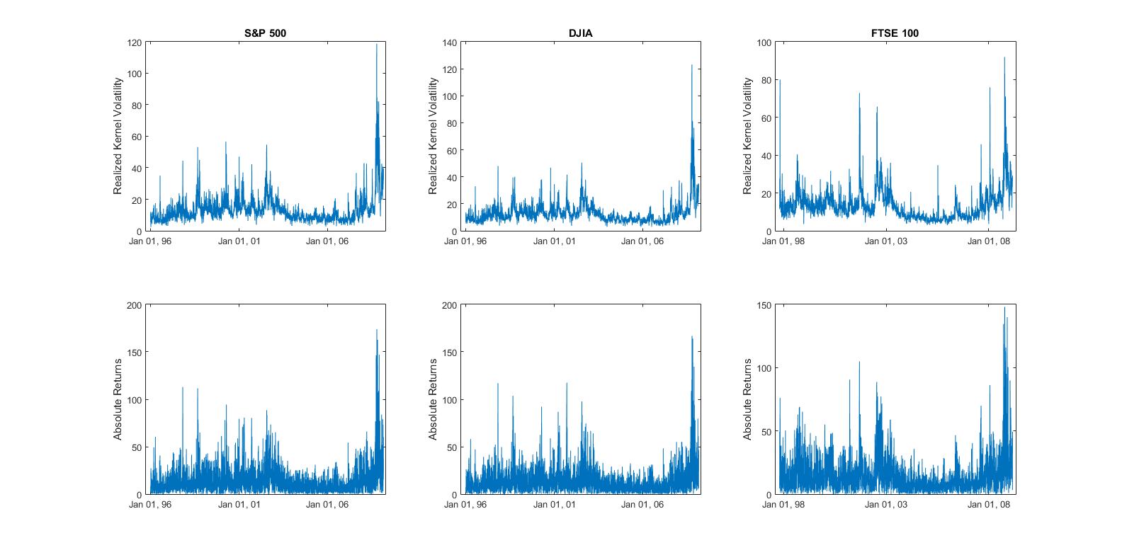
Figure 6: Time series of realized volatilities and absolute returns of S&P 500, DJIA, FTSE 100

For all the time series, we run 150,000 iterations of the algorithm described in Section 3 and then discard the first 30,000 of them as burn-in. In Table 2 we report, for all the time series, the estimates of the conditional mean parameters and the 95% credible intervals obtained with our model together with the maximum likelihood estimates of the same parameters and the corresponding standard errors obtained from the LN1-vMEM. In all the analyses, all the effective sample sizes of the variables obtained from the MCMC simulations are bigger than 500. In Table 3 we report the Log-Predictive scores and Log-Pseudo Marginal Likelihoods of the DPMLN2-vMEM and the LN1-vMEM. For the sake of brevity, we will plot hereafter only the traces, histograms and autocorrelation functions of the elements of the $\bm{\omega}$ vector (Figure 7), the estimations of the joint density and its marginals (Figure 8) and the traces of the total number of components (Figure 9) obtained analysing the time series of the S&P 500 index with DPMLN2-vMEM and LN1-vMEM. Very similar figures have been obtained for other parameters and for the other two time series.

Table 2: Posterior mean, 95% credible intervals, MAP estimates and corresponding standard error, for the parameters of the conditional mean.

	S&P 500		DJIA		FTSE 100
	MCMC Est.	MAP Est.	MCMC Est.	MAP Est.	MCMC Est.	MAP Est.
	(95% C.I.)	(S.d.)	(95% C.I.)	(S.d.)	(95% C.I.)	(S.d.)
$\omega_{1}$	0.0797	-0.0361	0.0200	-0.1158	0.0688	-0.0486
	$\left(-0.1290,0.3129\right)$	0.2475	$\left(-0.3079,0.3068\right)$	0.2527	$\left(-0.1119,0.2623\right)$	0.2156
$\omega_{2}$	0.3984	0.4686	0.3963	0.4520	0.1580	0.2089
	$\left(0.2834,0.5229\right)$	0.0604	$\left(0.2825,0.5171\right)$	0.0572	$\left(0.0914,0.2311\right)$	0.0401
$\beta_{1}$	0.7217	0.6379	0.6220	0.6387	0.6940	0.6629
	$\left(0.6505,0.7843\right)$	0.0524	$\left(0.5292,0.7055\right)$	0.0525	$\left(0.6223,0.7587\right)$	0.0624
$\beta_{2}$	0.5797	0.5604	0.5722	0.5622	0.7078	0.6735
	$\left(0.5404,0.6173\right)$	0.0157	$\left(0.5321,0.6113\right)$	0.0154	$\left(0.6700,0.7428\right)$	0.0125
$\alpha_{11}$	-0.0442	-0.1131	-0.0530	-0.0925	-0.0261	-0.0574
	$\left(-0.0686,-0.0202\right)$	0.0230	$\left(-0.0828,-0.0235\right)$	0.0251	$\left(-0.0556,0.0033\right)$	0.0282
$\alpha_{21}$	0.0397	0.0394	0.0355	0.0369	0.0271	0.0326
	$\left(0.0296,0.0502\right)$	0.0053	$\left(0.0262,0.0450\right)$	0.0048	$\left(0.0182,0.0361\right)$	0.0046
$\alpha_{12}$	0.3353	0.5917	0.4518	0.5611	0.3533	0.5139
	$\left(0.2651,0.4150\right)$	0.0754	$\left(0.3554,0.5564\right)$	0.0761	$\left(0.2694,0.4448\right)$	0.0970
$\alpha_{22}$	0.3491	0.3625	0.3608	0.3641	0.2519	0.2758
	$\left(0.3151,0.3845\right)$	0.0151	$\left(0.3252,0.3973\right)$	0.0145	$\left(0.2195,0.2870\right)$	0.0125

Table 3: Log-Predictive Scores (LPS) and Log Pseudo Marginal Likelihoods (LPML) for parametric and semiparametric models, for all the three series.

	S&P 500	DJIA	FTSE 100
LN1-vMEM LPS	6.1795	6.0238	6.1318
DPMLN2-vMEM LPS	6.0176	5.8676	5.9124
LN1-vMEM LPML	6.1882	6.0270	6.1349
DPMLN2-vMEM LPML	6.0370	5.8952	5.9394

Figure 7: MCMC traces, posterior histograms and ACFs of the components of the post-processed vector $\bm{\omega}$. The green lines in the histogram represent the 95% C.I.

Figure 8: Estimated joint and marginal densities of the innovations over the estimated innovations. On the upper row there are the results obtained with the DPMLN2-vMEM, on the lower row the ones obtained with LN1-vMEM

Figure 9: The upper plot shows the traces of total number of components and of the number of active components at each step. The lower plot shows the corresponding running averages.

From Figure 7 it can be seen that, although there is some autocorrelation the traces of the MCMC simulations have all reached convergence and the posterior histograms look informative.

For all the three time series and both the models considered, we obtain some common qualitative features of the point estimates. First of all the $\beta$s are always the biggest coefficients, meaning that the factor that influences the most the evolution of the conditional mean is always its lagged realization. Second, the estimates of the coefficients of the second column of matrix $\mathbf{A}$ are always bigger, in absolute value, than the ones in the first column of the same matrix. This suggests that the lagged realizations of the realized kernel volatility influence the evolution of both the components of the conditional mean vector more than the lagged realizations of the absolute returns. This fact, that could look strange at first sight, simply means that the lagged observation of the realized volatility contains more information on the present realization of the conditional mean of the absolute returns than the lagged absolute returns and this can be viewed as a further proof of the fact that the realized volatilities are more informative about the latent volatility than the absolute returns. Furthermore the $\alpha_{11}$ coefficient is always negative meaning that the conditional mean of the absolute returns depends inversely from the lagged realizations of the absolute returns.

In all the empirical analyses we tried there have always been about the same average number of active and total components of the DPM, for all the time series. Furthermore for all the time series there are always at least eight active components of the DPM for the whole MCMC run. The sum of the average of the weights of these components is always bigger than 0.99, meaning that, even in the MCMC steps in which there are more components, the first eight are dominant.

Regarding the approximation of the distribution of the data obtained with the DPMLN2-vMEM and with the LN1-vMEM, Figure 8 suggets that our semiparametric model outperforms its parametric counterpart. This can be perceived from the graphs of the joint distribution, especially near the $y$-axis, but it becomes clearer looking at the graphs of the marginals: whilst the second marginals are indeed very similar, the approximation of the first marginal (second column of the figure) obtained with DPMLN2-vMEM is much better than the one obtained with LN1-vMEM, since the DPM model seems to better approximate the data close to zero. For what it takes the predictive performances in the sample, Table 3 suggests that DPMLN2-vMEM performs better than LN1-vMEM.

6 Conclusions

We proposed a Bayesian semiparametric vMEM for non-negative multivariate random vectors, a relevant setting in many financial applications. Our contribution is the formulation of a statistical model that is (i) not bounded to special parametric forms of the error term distribution, known to be a quite strong restriction with multivariate data, and (ii) subject to weaker assumptions than the other semiparametric approaches in the literature, based on the Generalized Method of Moments.

In more details, the innovation term of our vMEM follows a location-scale DPM of multivariate log-normal distributions. By exploiting a parameter-expanded unconstrained version of the model, we are able to simplify the computational difficulties arising from the constraints to the positive orthant and we formalize an efficient slice sampler for posterior inference. The proposed model shows better fitting and predictive performances than its parametric counterpart in both the simulations and in the empirical study on the interaction between daily absolute returns and realized kernel volatilities.

Further developments of interest include (i) a refinement of the sampling technique with sparsity-driven efficiencies that can manage time series in high dimension, (ii) a more complex specification of the conditional mean, with the purpose of comparing volatility proxies through more elaborated models with non-linearities in the dynamics and (iii) the adoption of the proposed model for other applications of interest, e.g. for the analysis of spillover effects between market indices.

References

- Aït-Sahalia et al. (2010) Yacine Aït-Sahalia, Jianqing Fan, and Dacheng Xiu. High-frequency covariance estimates with noisy and asynchronous financial data. Journal of the American Statistical Association, 105(492):1504–1517, 2010.
- Andersen and Bollerslev (1998) T.G. Andersen and T. Bollerslev. Answering the skeptics: Yes, standard volatility models do provide accurate forecasts. International Economic Review, pages 885–905, 1998.
- Antoniak (1974) C.E. Antoniak. Mixtures of dirichlet processes with applications to bayesian nonparametric problems. The Annals of Statistics, pages 1152–1174, 1974.
- Barndorff-Nielsen et al. (2008) Ole E Barndorff-Nielsen, Peter Reinhard Hansen, Asger Lunde, and Neil Shephard. Designing realized kernels to measure the ex post variation of equity prices in the presence of noise. Econometrica, 76:1481–1536, 2008.
- Cifarelli and Regazzini (1990) D.M. Cifarelli and E. Regazzini. Distribution functions of means of a dirichlet process. The Annals of Statistics, pages 429–442, 1990.
- Cipollini et al. (2006) F. Cipollini, R.F. Engle, and G.M. Gallo. Vector multiplicative error models: representation and inference. Technical report, National Bureau of Economic Research, 2006.
- Cipollini et al. (2013) F. Cipollini, R.F. Engle, and G.M. Gallo. Semiparametric vector mem. Journal of Applied Econometrics, 28(7):1067–1086, 2013.
- Corsi et al. (2015) Fulvio Corsi, Stefano Peluso, and Francesco Audrino. Missing in asynchronicity: a kalman-em approach for multivariate realized covariance estimation. Journal of Applied Econometrics, 30(3):377–397, 2015.
- Dalal and Hall (1980) SR Dalal and Gaineford J Hall. On approximating parametric bayes models by nonparametric bayes models. The Annals of Statistics, pages 664–672, 1980.
- Engle (2002) R.F. Engle. New frontiers for arch models. Journal of Applied Econometrics, 17(5):425–446, 2002.
- Engle and Gallo (2006) R.F. Engle and G.M. Gallo. A multiple indicators model for volatility using intra-daily data. Journal of Econometrics, 131(1):3–27, 2006.
- Engle et al. (2012) R.F. Engle, G.M. Gallo, and M. Velucchi. Volatility spillovers in east asian financial markets: a mem-based approach. Review of Economics and Statistics, 94(1):222–223, 2012.
- Engle et al. (2009) R.F.t Engle, G.M. Gallo, and M. Velucchi. A mem-based analysis of volatility spillovers in east asian financial markets. 2009.
- Engle and Russell (1998) Robert F Engle and Jeffrey R Russell. Autoregressive conditional duration: a new model for irregularly spaced transaction data. Econometrica, pages 1127–1162, 1998.
- Giovannetti and Velucchi (2011) G. Giovannetti and M. Velucchi. A mem analysis of african financial markets. In New Perspectives in Statistical Modeling and Data Analysis, pages 319–328. Springer, 2011.
- Hall (2005) Alastair R Hall. Generalized method of moments. Oxford university press, 2005.
- Jensen and Maheu (2010) Mark J Jensen and John M Maheu. Bayesian semiparametric stochastic volatility modeling. Journal of Econometrics, 157(2):306–316, 2010.
- Jensen and Maheu (2018) Mark J Jensen and John M Maheu. Risk, return and volatility feedback: A bayesian nonparametric analysis. Journal of Risk and Financial Management, 11(3):52, 2018.
- Jensen and Maheu (2014) M.J. Jensen and J.M. Maheu. Estimating a semiparametric asymmetric stochastic volatility model with a dirichlet process mixture. Journal of Econometrics, 178:523–538, 2014.
- Johnson et al. (1997) N.L. Johnson, S. Kotz, and N. Balakrishnan. Discrete multivariate distributions. Wiley New York, 1997.
- Johnson et al. (2000) N.L. Johnson, S. Kotz, and N. Balakrishnan. Continuous multivariate distributions. Wiley New York, 2000.
- Kalli et al. (2011) M. Kalli, J.E. Griffin, and S.G. Walker. Slice sampling mixture models. Statistics and computing, 21(1):93–105, 2011.
- Kalli et al. (2013) M. Kalli, S.G Walker, and P. Damien. Modeling the conditional distribution of daily stock index returns: An alternative bayesian semiparametric model. Journal of Business & Economic Statistics, 31(4):371–383, 2013.
- Kim et al. (1998) Sangjoon Kim, Neil Shephard, and Siddhartha Chib. Stochastic volatility: likelihood inference and comparison with arch models. The Review of Economic Studies, 65(3):361–393, 1998.
- Korwar et al. (1973) Ramesh M Korwar, Myles Hollander, et al. Contributions to the theory of dirichlet processes. The Annals of Probability, 1(4):705–711, 1973.
- Lijoi A. (2004) Regazzini E. Lijoi A. Means of a dirichlet process and multiple hypergeometric functions. Annals of probability, pages 1469–1495, 2004.
- Liu C. (1998) Wu Y.N. Liu C., Rubin D.B. Parameter expansion to accelerate em: the px-em algorithm. Biometrika, 85(4):755–770, 1998.
- Liu J.S. (1999) Wu Y.N. Liu J.S. Parameter expansion for data augmentation. Journal of the American Statistical Association, 94(448):1264–1274, 1999.
- Muliere and Tardella (1998) P. Muliere and L. Tardella. Approximating distributions of random functionals of ferguson-dirichlet priors. Canadian Journal of Statistics, 26(2):283–297, 1998.
- Nieto-Barajas et al. (2014) Luis E Nieto-Barajas, Alberto Contreras-Cristán, et al. A bayesian nonparametric approach for time series clustering. Bayesian Analysis, 9(1):147–170, 2014.
- Parkinson (1980) Michael Parkinson. The extreme value method for estimating the variance of the rate of return. Journal of Business, 53:61–65, 1980.
- Peluso et al. (2014) Stefano Peluso, Fulvio Corsi, and Antonietta Mira. A bayesian high-frequency estimator of the multivariate covariance of noisy and asynchronous returns. Journal of Financial Econometrics, 13(3):665–697, 2014.
- Peluso et al. (2017) Stefano Peluso, Antonietta Mira, and Pietro Muliere. Robust identification of highly persistent interest rate regimes. International Journal of Approximate Reasoning, 83:102–117, 2017.
- Peluso et al. (2019) Stefano Peluso, Antonietta Mira, and Pietro Muliere. Conditionally gaussian random sequences for an integrated variance estimator with correlation between noise and returns. Applied Stochastic Models in Business and Industry, 35(5):1282–1297, 2019.
- Pitman (2002) J. Pitman. Combinatorial stochastic processes. Technical report, U.C. Berkeley Department of Statistics, 2002.
- Regazzini et al. (2003) E. Regazzini, A. Lijoi, and I. Prünster. Distributional results for means of normalized random measures with independent increments. Annals of Statistics, pages 560–585, 2003.
- Roberts and Rosenthal (2007) G.O. Roberts and J.S. Rosenthal. Coupling and ergodicity of adaptive markov chain monte carlo algorithms. Journal of applied probability, pages 458–475, 2007.
- Shephard and Sheppard (2010) Neil Shephard and Kevin Sheppard. Realising the future: forecasting with high-frequency-based volatility (heavy) models. Journal of Applied Econometrics, 25(2):197–231, 2010.
- Solgi and Mira (2013) R. Solgi and A. Mira. A bayesian semiparametric multiplicative error model with an application to realized volatility. Journal of Computational and Graphical Statistics, 22(3):558–583, 2013.
- Taylor and Xu (2017) Nick Taylor and Yongdeng Xu. The logarithmic vector multiplicative error model: an application to high frequency nyse stock data. Quantitative Finance, 17(7):1021–1035, 2017.
- Van Dyk D.A. (2001) Meng X.L. Van Dyk D.A. The art of data augmentation. Journal of Computational and Graphical Statistics, 10(1), 2001.
- Virbickaitė et al. (2016) Audronė Virbickaitė, M Concepción Ausín, and Pedro Galeano. A bayesian non-parametric approach to asymmetric dynamic conditional correlation model with application to portfolio selection. Computational Statistics & Data Analysis, 100:814–829, 2016.
- Walker (2007) S.G. Walker. Sampling the dirichlet mixture model with slices. Communications in Statistics: Simulation and Computation, 36(1):45–54, 2007.
- Yang et al. (2010) Mingan Yang, David B Dunson, and Donna Baird. Semiparametric bayes hierarchical models with mean and variance constraints. Computational statistics & data analysis, 54(9):2172–2186, 2010.
- Zaharieva et al. (2020) Martina Danielova Zaharieva, Mark Trede, and Bernd Wilfling. Bayesian semiparametric multivariate stochastic volatility with application. Econometric Reviews, pages 1–24, 2020.