A new constant behind the rotational velocity of galaxies

Abstract

The present work is devoted to studying the dynamical evolution of galaxies in scalar-Gauss-Bonnet  gravity and its relationship with the MOND paradigm. This study is useful for giving meaning to the presence of a new gravitational constant. The stability of dark matter is strongly dependent on matter density. We are interested in calculating the maximum rotational velocity of galaxies. We show that rotating galaxies can be described by a new parameter that depends both on the minimum value of scalar fields and on the effective mass of this field. According to observational data, we have shown that this parameter is a constant.

Keywords: Dark matter, Galaxies, Einstein-Gauss-Bonnet gravity.

1 Introduction

Recently, several models of extended or modified gravity theories were proposed [1], to explain the missing gravity problem [2], one of the major problems in modern cosmology. According to Lovelock theorem [3], the Gauss-Bonnet (GB) gravity is introduced only in case $D>4$. In four-dimensional spacetime, the GB term does not contribute to the gravitational dynamics. Recently, there has been renewed interest in the GB gravity, D. Glavan and C. Lin [4] proposed a novel 4-dimensional Einstein-Gauss-Bonnet (EGB) gravity, which has attracted great attention. Their idea is to multiply the GB term by $1/(D-4)$ before taking the limit. This offers a new 4-dimensional gravitational theory with only two dynamical degrees of freedom by consider the $D\longrightarrow 4$ limit of EGB gravity in $D>4$ dimensions [5], which is in contradiction with Lovelock theorem. However, it was shown in several papers that perhaps the idea of the limit $D\longrightarrow 4$ is not clearly defined. Several ideas have been proposed to remedy this inconsistency and the absence of a proper action [6, 7, 8, 9]. Although the EGB gravity is currently debatable, the spherically symmetric black hole solution is still meaningful and worthy of study [10]. There is a little work on the study of dark matter in the context of EGB gravity [11]. Note that the $R^{2}$ gravity models are an increasingly important area of research to study the missing gravity problem [12]. Since GB contains an $R^{2}$ term, in this case, we can propose that GB gravity generalize $R^{2}$ gravity. Khoury and Weltman [13] proposed a new coupling that gives to the scalar field a mass depending on the local density of matter. The modified Newtonian dynamics (MOND) an effective theory paradigm proposed to explain the problem of flat rotation curve of spiral galaxies. It constitutes an alternative to the concept of dark matter [14]. MOND constitutes a modification to Newtonian dynamics in the limit of low accelerations. This would mean that MOND might emerge as an approximate consequence of some deeper physical theory [15]. In the present paper, we consider a model of a scalar field $\phi$ in the context of EGB gravity. This scalar field will describe the dark matter. Thus this model very robustly leads to the maximum values of rotational velocity of galaxies and dust for scalar field potentials.
The MOND model enables a broadening of the range of scales that are theoretically well understood, from the kpc scales of galactic bars to the Gpc scale of the local void and the Hubble tension [16]. MOND can account for the Hubble tension by means of outflow from a large local supervoid, which has been observed and is known as the KBC void [17]. While outflows from voids are expected in $\Lambda$CDM, structure formation would be enhanced in MOND, allowing it to explain the formation of the KBC void even though $\Lambda$CDM cannot [19]. A number of theories of gravity have studied dark matter in the regime of galaxies according to the relativistic MOND theory [20, 21]. MOND can also account for the massive high-redshift galaxy cluster collision known as El Gordo, which contradicts $\Lambda$CDM at high significance [22]
A group of galaxies was studied using the MOND and the dark haloes, in view of two suggested explanations for the discrepancy between the luminous mass and the conventional dynamical mass of galaxies [23, 24, 25].
This paper is organized as follows. In the next section, we introduce the model of the scalar field $\phi$ minimally coupled to EGB gravity. Section 3 is devoted to analyzing the mass of the scalar field. In section 4, we discuss the stability of EGB  gravity. In section 5, we perform analytic analyses of the rotation curve of the galaxies. The last section is devoted to the conclusion.

2 Minimally coupled to EGB  gravity

Recently, there has been a renewed interest in the relationship between dark matter and the scalaron mass [26, 27]. Consider now the scalar-Gauss-Bonnet gravity in $4$-dimensions [28, 29]:

$$S=\int d^{4}x\sqrt{-g}\left(\frac{M_{p}^{2}}{2}R+f\left(\phi\right)\mathcal{G}-\frac{1}{2}g^{\mu\nu}\partial_{\mu}\phi\partial_{\nu}\phi-V\left(\phi\right)\right),$$ (2.1)

where $M_{p}^{2}=\frac{c^{4}}{8\pi G}$, $R$ is the Ricci scalar, and $f\left(\phi\right)$ is the Gauss-Bonnet coupling function with dimensions of $\left[length\right]^{2}$, that represent ultraviolet (UV) corrections to Einstein theory. In the above equation $\left(\mu,\nu\right)=\left(0,1,2,3\right)$. We define the Gauss-Bonnet invariant as

$$\mathcal{G}\equiv R^{2}-4R_{\mu\nu}R^{\mu\nu}+R_{\mu\nu\rho\sigma}R^{\mu\nu\rho\sigma}.$$ (2.2)

The variation with respect to the field $\phi$ gives us the equation of motion for the scalaron field

$$\square\phi-\partial_{\phi}V\left(\phi\right)+\mathcal{G}\partial_{\phi}f\left(\phi\right)=0.$$ (2.3)

The variation of the action over the metric $g_{\mu\nu}$ simplified by the Bianchi identity gives

$$0 = M_{p}^{2}\left(R^{\mu\nu}-\frac{1}{2}g^{\mu\nu}R\right)+\frac{1}{2}\partial^{\mu}\phi\partial^{\nu}\phi-\frac{1}{4}g^{\mu\nu}\partial_{\rho}\phi\partial^{\rho}\phi+\frac{1}{2}g^{\mu\nu}\left(-V\left(\phi\right)+f\left(\phi\right)\mathcal{G}\right)$$

$$f\left(\phi\right)\left(-2RR^{\mu\nu}+R_{\text{ \ }\rho}^{\mu}R^{\nu\rho}-2R^{\mu\rho\sigma\tau}R_{\text{ \ }\rho\sigma\tau}^{\nu}+4R^{\mu\rho\sigma\tau}R_{\text{ \ }\rho\sigma\tau}^{\nu}\right)$$

$$+\left(2R\nabla^{\mu}\nabla^{\nu}-2g^{\mu\nu}R\nabla^{2}-4R^{\nu\rho}\nabla_{\rho}\nabla^{\mu}-4R^{\mu\rho}\nabla_{\rho}\nabla^{\nu}\right)f\left(\phi\right)$$

$$+4\left(\nabla^{2}f\left(\phi\right)\right)R^{\mu\nu}+4g^{\mu\nu}\left(\nabla_{\rho}\nabla_{\sigma}f\left(\phi\right)\right)R^{\rho\sigma}-4\left(\nabla_{\rho}\nabla_{\sigma}f\left(\phi\right)\right)R^{\mu\rho\nu\sigma}.$$

The metric of a spatially flat homogeneous and isotropic universe in FLRW model is given by:

$$ds^{2}=-dt^{2}+a^{2}(t)\sum_{i=1}^{3}\left(dx^{i}\right)^{2},$$ (2.5)

where $a(t)$ is a dimensionless scale factor, from which we define the Ricci scalar $R$ and the GB invariant $\mathcal{G}$ in FLRW geometry as

$$R=6\left(2H^{2}+\dot{H}\right)\text{ \ \ \ \ }\mathcal{G}=24H^{2}\left(\dot{H}+H^{2}\right).$$ (2.6)

We start by considering $\phi=\phi\left(t\right)$. So, Eq.(2) is written as

$$\frac{1}{2}\dot{\phi}^{2}+24H^{3}f^{\prime}\left(\phi\right)\dot{\phi}+V\left(\phi\right)=3M_{p}^{2}H^{2},$$ (2.7)

where $\dot{\phi}\equiv\partial_{t}\phi$, $f^{\prime}\left(\phi\right)\equiv\partial_{\phi}f\left(\phi\right)$, and $H\equiv\dot{a}/a$ is the Hubble parameter. The scalar term vanishes if $\dot{\phi}=0$, leading to $V\left(\phi=constant\right)=3M_{p}^{2}H^{2}$ (the cosmic critical density). The solution Eq.(2.7) is then evaluated in the form of an energy equation. There is a dark matter sector with $\Omega_{DM}=\dot{\phi}^{2}/6M_{p}^{2}H^{2}$ and a dark energy sector with $\Omega_{DE}=V\left(\phi\right)/3M_{p}^{2}H^{2}$. For interaction between these sectors, we have $\Omega_{I}=24Hf^{\prime}\left(\phi\right)\dot{\phi}/3M_{p}^{2}$. The fraction of dark matter is $\Omega_{DM}=1-\Omega_{DE}-\Omega_{I}$. It is possible, that for appropriate choices of the potential and the coupling function, that competition between these terms leads to a minimum in the effective potential. We consider in this work the dilatonic-type:

$$V\left(\phi\right)=V_{0}e^{-k\phi}\text{, \ }f\left(\phi\right)=f_{0}e^{+k\phi},$$ (2.8)

in this case, we refer to the scalaron as a dilaton field. Indeed, the coupling function remains invariant under the simultaneous sign change $\left(k,\phi\right)\rightarrow\left(-k,-\phi\right)$. The equatios of motion (Eq.2.3) is invariant under the transformation $V\left(\phi\right)\longleftrightarrow-\mathcal{G}f\left(\phi\right)$. In what follows, we shall assume that the term$-\mathcal{G}f\left(\phi\right)$ represents the second term in the effective potential. In that case the harmonic term dominates the potential, so one can approximate the equation of motion to find a damped harmonic oscillation [28].

3 The scalaron mass

Next, we study the mass of the scalar field which will describe the mass of dark matter. In order to find an explicit expression for the scalaron mass, we need to consider an effective potential in the equation of motion (Eq.2.3), which can be written as the Klein Gordon equation in the FLRW metric as:

$$\ddot{\phi}+3H\dot{\phi}+\partial_{\phi}V\left(\phi\right)-\mathcal{G}\partial_{\phi}f\left(\phi\right)=0.$$ (3.1)

Let us now use the above expressions to examine the evolution of the scalaron. Observe that the term $V\left(\phi\right)-\mathcal{G}f\left(\phi\right)$ acts as the effective potential for the perturbations. The effective potential [30, 31] that includes the GB term can be written as:

$$V_{eff}=V\left(\phi\right)-\mathcal{G}f\left(\phi\right).$$ (3.2)

We notice that the effective potential of the scalaron includes the Gauss-Bonnet coupling and the Gauss-Bonnet invariant. In other words, the Gauss-Bonnet term affects the potential structure of the scalaron, so the scalaron mass depends on the matter contribution. The particles of the field $\phi$ come from the fluctuation around the minimum of the effective potential $V_{eff}(\phi)$. Using (2.8), the second derivative of the effective potential Using $\phi$ is

$$\frac{\partial^{2}}{\partial\phi^{2}}V_{eff}=k^{2}V_{0}e^{-k\phi}-k^{2}\mathcal{G}f_{0}e^{+k\phi}.$$ (3.3)

As before the existence of a minimum in the effective potential requires $\mathcal{G}\neq 0$. More precisely, we define the effective mass as a function of the field $\phi$

$$m_{eff}^{2}=\left.\frac{\partial^{2}}{\partial\phi^{2}}V_{eff}(R,\phi)\right|_{\phi=\phi_{\min}},$$ (3.4)

where $\phi_{\min}$ is the minimum value of the scalaron $\phi$. The effective mass is then given by

$$m_{eff}=k\sqrt{V_{0}e^{-k\phi_{\min}}-\mathcal{G}f_{0}e^{+k\phi_{\min}}}.$$ (3.5)

When the minimum of the scalaron is very small, the solution could be given by $m_{eff}=k\sqrt{V_{0}-\mathcal{G}f_{0}}$. The domain of validity of the fluid description of dark matter is when $m_{eff}$ is real. One finds that $\mathcal{G}$ has the bound

$$\mathcal{G}\leq\frac{V_{0}}{f_{0}}e^{-2k\phi_{\min}}.$$ (3.6)

If the condition is satisfied everywhere in spacetime, then the adiabatic approximation will be good everywhere. In particular, considering the maximum value of $\mathcal{G}$ is:

$$\mathcal{G}_{\max}=\frac{V_{0}}{f_{0}}e^{-2k\phi_{\min}}.$$ (3.7)

For $\mathcal{G=G}_{\max}$, the scalaron mass will be zero. The above inequality Eq.(3.7) can be written as

$$q\geq\frac{-V_{0}}{24H^{4}f_{0}}e^{-2k\phi_{\min}},$$ (3.8)

where $q\equiv-1-\dot{H}/H^{2}=-a\ddot{a}/\dot{a}^{2}$ is the deceleration parameter. We mention that according to Eq.(3.8), even if $\mathcal{G}$ $=\mathcal{G}_{\max}$, the asymptotic value of $q$ depends on the model parameters $V_{0}$ and $f_{0}$. Furthermore the isolated points where $q=q_{\min}$ constitute a set of measure zero and do not contribute to $m_{eff}$.

4 Dark matter stability analysis

Let us describe the effective potential in an environment that surrounds the matter. The GB invariant can be greatly simplified to the matter density $\rho$ [30], giving

$$\mathcal{G}=\rho.$$ (4.1)

Therefore, in order to satisfy Eq.(3.6) one must set that $V_{0}$ and $f_{0}$ have the same sign. From Eqs.(2.8,3.2,3.7,4.1) and we adopt that $\mathcal{G}_{\max}=\rho_{\max}$ we finally obtain

$$V_{eff}=f_{0}e^{-k\phi}\left(\rho_{\max}e^{2k\phi_{\min}}-\rho e^{2k\phi}\right),$$ (4.2)

this expression is comparable to that found by [30]. At low $k\phi$, the effective potential can be approximated by $V_{0eff}$. In the high $k\phi$ regime, $V_{eff}$ to $V_{0}\exp(k\phi)$. Our discussion of stability in the following sections will be valid for $m_{eff}^{2}\left(\phi\right)>0$. We can then express the mass $m_{eff}$ as a function of the matter energy density

$$m_{eff}^{2}=k^{2}f_{0}e^{-k\phi_{\min}}\left(\rho_{\max}-\rho\right),$$ (4.3)

where we have taken into account that $\rho_{\max}=\frac{V_{0}}{f_{0}}e^{-2k\phi_{\min}}$. The mass of small fluctuations is an increasing function of the matter energy density. At low density, the effective mass can be approximated by $k^{2}V_{0}e^{-3k\phi_{\min}}$. In the high-density region, $m_{eff}$ to $0$, corresponding to the dark matter halos around galaxies. To be more precise, dark matter is very important in the extremities of the galaxy when $\rho\sim 0$. Apart from the evolution of the scalaron that was extracted above, the other important consequence is that when the matter energy density becomes maximal, the mass of this field will be zero. The effective pressure and density are $p_{eff}=-V\left(\phi\right)+f\left(\phi\right)\rho$ and $\rho_{eff}=V\left(\phi\right)$, respectively. The effective equation of state for this system is given by:

$$\omega_{eff}\equiv\frac{p_{eff}}{\rho_{eff}}=-1+\frac{\rho}{\rho_{\max}}e^{2k\left(\phi-\phi_{\min}\right)}.$$ (4.4)

We mention that the $\omega_{eff}$ lies in the density $\rho$ and the scalaron $\phi$. If $V_{0}>0$, the pressure for this system will be negative. The system will be stable if

$$c_{eff}^{-2}\equiv\frac{d\rho_{eff}}{dp_{eff}}>0,$$ (4.5)

where $c_{eff}$ is the effective sound speed. This equation gives a simple prescription for computing when a given theory will be stable. We calculate $c_{eff}$ for a fixed density, allowing us to find that $\omega_{eff}=1/c_{eff}^{2}$. We mention that for $\omega_{eff}=0$, we find that $\rho_{\max}=\rho e^{2k\left(\phi-\phi_{\min}\right)}$. Even if $\phi\sim\phi_{\min}$, one obtains the asymptotic value $\rho\simeq\rho_{\max}$. Additionally, to assess possible behaviors of the sound speed squared and $\omega_{eff}$, we remark that the stable regime arises in the case

$$\rho_{\max}<\rho e^{2k\left(\phi-\phi_{\min}\right)}.$$ (4.6)

In this expression, $k$ should be positive so that the theory will be stable (since $\phi>\phi_{\min}$). If $k<0$, the mass $m_{eff}$ correspond to the tachyonic instability. Inserting $\rho<\rho_{\max}$ into Eq.(4.6) we get the result that $1<\frac{\rho_{eff}}{\rho}<e^{2k\left(\phi-\phi_{\min}\right)}$, it is necessary that $k>0$. In the regime of large densities, we have $\phi>\phi_{\min}$. If $\phi\gg\phi_{\min}$, the effective sound speed can be greatly simplified, giving $c_{eff}^{2}>0$. In summary, this analysis shows that the EGB dark matter lies in the stable regime. Since the right hand side involves exponential factors, we expect that the field $\phi$ to evolve by a logarithmic function of the matter density.

5 Rotation curves from MOND and the relation to EGB

It is well known that the orbital velocities $v$ of planets in planetary systems and moons orbiting planets decline with distance according to Kepler’s third law [32] $v^{2}=\frac{GM}{r},$ with $G\approx 6,67\times 10^{-11}m^{3}Kg^{-1}s^{-2}$. In contrast, stars revolve around their galaxy’s center at equal or increasing speed over a large range of distances [33]. The rotational speeds of stars inside the galaxies do not follow the rules found in smaller orbital systems. A solution to this conundrum is to suppose the existence of dark matter and to tune its distribution from the galaxy’s center out to its halo based on the observed kinematics [34]. The effective potential can be used to determine the orbits of planets [35], also in the cosmological evolution analysis of the chameleon field, allowing the detection of dark energy in orbit [36]. According to the MOND theory [14], the rotational velocity of stars around a galaxy at large distances is:

$$v_{0}^{4}=GMa_{0}.$$ (5.1)

where $a_{0}\approx 1,2\times 10^{-10}ms^{-2}$ and $M$ is the total mass of a galaxy. It is treated as a point mass at its centre, providing a crude approximation for a star in the outer regions of a galaxy. The Eq.(5.1) predicts that the rotational velocity is constant out to an infinite range and that the rotational velocity doesn’t depend on a distance scale, but on the magnitude of the acceleration $a_{0}$. We suppose that the constant $a_{0}$ ni more constant, after seeing the form of galaxy rotation curves in MOND [15]. We start by changing

$$v_{0}^{4}\rightarrow GM\left(\frac{GM}{f_{0}}\right),$$ (5.2)

where $f_{0}$ has dimensions of $\left[length\right]^{2}$. We can write that the rotational velocity of a galaxy is:

$$v^{2}\left(r\right)=\frac{GMk}{m_{eff}}e^{-\frac{k\phi_{\min}}{2}}\sqrt{\rho_{\max}-\rho\left(r\right)},$$ (5.3)

where $\rho$ is the local matter energy density, $\rho_{\max}$ is the maximum density of the galaxy and $M$ is its mass. We consider a disk of radius $r$ with its center at the galactic center. This modification based on EGB gravity instead of Newton’s gravity (as in the case of MOND theory), will later introduce a relativistic term to the potential. Moreover, the study of relativistic treatment within the framework of MOND theory is treated in [16, 18]. The choice of this potential has several advantages, since it generalizes the Newtonian potential and it has a relation with the potential of MOND theory [14]. The potential above has a relativistic aspect which is related to the parameters of EGB gravity. The term $\sqrt{1-\frac{\rho\left(r\right)}{\rho_{\max}}}$ represents the relativistic part of this potential. The description of the rotation of galaxies in the relativistic EGB gravity is better compared to the Newtonian frame, and gives a complete dynamic in space-time. On the other hand, the MOND theory remains incomplete since it has a lack of relativistic treatment of the rotation of galaxies. Note that in the edges of the galaxy we take a low matter energy density $\rho\left(r_{\max}\right)\sim 0$, yielding:

$$V_{\max}\sim\left(GM\right)^{1/2}\left(\rho_{\max}\right)^{1/4}\theta_{0},$$ (5.4)

where $\theta_{0}=\left(ke^{-\frac{k\phi_{\min}}{2}}/m_{eff}\right)^{1/2}$. The parameter $\theta_{0}$ strongly affects the behavior of the velocity $V_{\max}$. The galaxy’s rotation curves remain almost constant or increasing at the edges of galaxies [33, 37, 38]. To describe the maximum rotational velocity of a galaxy, we use the speed $V_{\max}$ Eq.(5.4). which corresponds to an almost constant rotation if $\theta_{0}$ is fixed. In what follows, we will draw the curve of $\theta_{0}$ according to the observations. To determine the value of $\theta_{0}$, we study the maximum values of rotational velocity $V_{\max}$ of galaxies according to their density $\rho$ and the masse $M_{in}$ of galaxies. Using the observation results, we can determine the values of $\theta_{0}$ [39, 40, 41, 42]:

$$\theta_{0}\approx 8.167\times 10^{-6}\times V_{\max}\times\rho_{\max}^{-\frac{1}{4}}\times M^{-\frac{1}{2}}.$$ (5.5)

To find the value of $\theta_{0}$ we have to calculate $\left(M,\rho_{\max},V_{\max}\right)$ for some galaxies in the tables of the Appendix.

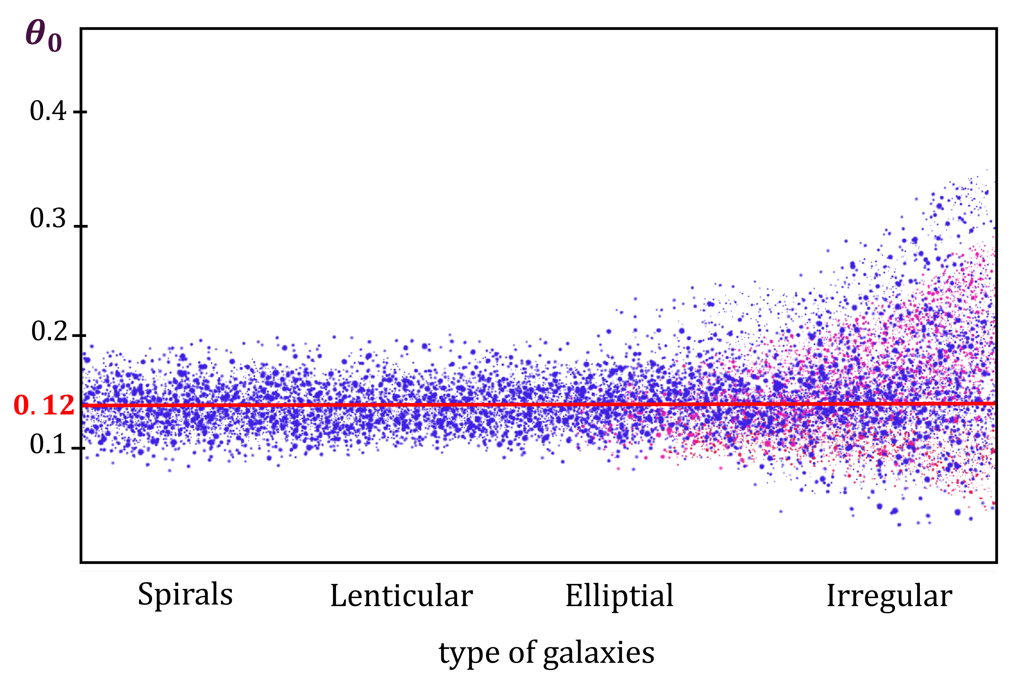
Figure 1: $\theta_{0}$ vs type of galaxies. These points are obtained from observations [33]. Notice that the values of $\theta_{0}$ are almost constant ($\theta_{0}\approx 0.12$).

According to Figure (1), the parameter $\theta_{0}$ permit us to determine the rotational velocity of galaxies. The values of $\theta_{0}$ are very close under wide range of conditions, but there are exceptions like dwarf spheroidal galaxies.

6 Summary

We have presented a study that is designed to describe dark matter in Einstein-Gauss-Bonnet (EGB) gravity coupled with scalar fields. We also analyzed the effects of the GB invariant on the evolution of effective potential. Also, the stability of dark matter was discussed in the context of this model. We have presented an explicit procedure to construct the effective equation of state describing the scalar fields. The potential describes the rotation of galaxies by two parameters $k$ and $m_{eff}$ introduced by EGB gravity. Indeed, these two parameters describe the dark matter hidden in galaxies. We have compared our results with observations. We have used the EGB gravity and MOND theory, in relationship with the field $\phi$ to provide a qualitative description of modified gravity. We found an expression of for how the rotation curve of a galaxy depends on the parameter $\theta_{0}$. We obtained a graph (Figure 1) of $\theta_{0}$ using the observational data (Appendix) which corresponds exactly to the evolution of the rotation of galaxies. We have shown that $\theta_{0}$ is an essential parameter, which is constant for spirals, lenticular and elliptical galaxies, but is no longer a constant for irregular and dwarf spheroidal galaxies. This shows that the parameter $\theta_{0}$ plays an important role in describing both the rotation and the type of galaxies. Future work will have to test if this model also corresponds to other observations like the CMB.

7 Appendix

Galaxy $$\rho(\times 10^{-22}kg/m^{2})$$

Milky Way

NGC 7331

NGC 4826

NGC 6503

NGC 7793

UGC 2885

NGC 253

NGC 925

NGC 2403

NGC 2841

NGC 2903

NGC 3198

NGC 5585

NGC 4321

Table 1: Large spirals galaxies

Galaxy $$\rho(\times 10^{-22}kg/m^{2})$$

NGC 4303

NGC 5055

NGC 4736

NGC 5194

NGC 4548

Table 2: Messier Spirals

Galaxy $$\rho(\times 10^{-22}kg/m^{2})$$

UGC 3993

NGC 7286

NGC 2768

NGC 3379

NGC 2434

NGC 4431

Table 3: Lenticular and Elliptical Galaxies

Galaxy $$\rho(\times 10^{-22}kg/m^{2})$$

WLM (DDO 221)

M81dWb

Holmberg II

NGC 3109

NGC 4789a

NGC 3034

Table 4: irregular dwarf galaxies

Galaxy $$\rho(\times 10^{-22}kg/m^{2})$$

Carina

Leo I

Draco

Fornax

Table 5: dwarf spheroidal galaxies (dSphs)

References

- [1] Amendola, Luca, et al. 2018, Living Rev. Relativ., 21.1 : 2.
- [2] Bertone, Gianfranco, and Dan Hooper. 2018, Rev. Mod. Phys., 90.4 : 045002.
- [3] Lovelock, D. 1971, J. Math. Phys., 12(3), 498-501.
- [4] Glavan, D., & Lin, C. 2020, Phys. Rev. Lett., 124(8), 081301.
- [5] Aoki, K., Gorji, M. A., & Mukohyama, S. 2020, Phys. Lett. B, 135843.
- [6] Bonifacio, J., Hinterbichler, K., & Johnson, L. A. 2020, Phys. Rev. D, 102(2), 024029.
- [7] Gürses, M., Şişman, T. Ç., & Tekin, B. 2020, Phys. Rev. Lett., 125(14), 149001.
- [8] Wang, D., & Mota, D. 2021, Phys. Dark Universe, 100813.
- [9] Wu, C. H., Hu, Y. P., & Xu, H. 2021, Eur. Phys. J. C, 81(4), 1-9.
- [10] Guo, M., & Li, P. C. 2020, Eur. Phys. J. C, 80(6), 1-8.
- [11] Meehan, M. T., & Whittingham, I. B. 2014, J. Cosmol. Astropart. Phys., 2014(12), 034.
- [12] Cembranos, Jose AR. 2009, Phys. Rev. Lett. 102.14 : 141301.
- [13] Khoury, Justin, and Amanda Weltman. 2004, Phys. Rev. D, 69.4 : 044026.
- [14] Milgrom, Mordehai. 1983, Astrophys. J., 270 : 365-370.
- [15] Milgrom, M. 2008. arXiv preprint arXiv, :0801.3133.
- [16] Banik, I., & Zhao, H. (2021), arXiv preprint arXiv:2110.06936.
- [17] Keenan, R. C., Barger, A. J., & Cowie, L. L. (2013), Astrophys. J., 775(1), 62.
- [18] Bekenstein, J. D. (2004), Phys. Rev. D, 70(8), 083509.
- [19] Haslbauer, M., Banik, I., & Kroupa, P. (2020), Mon. Not. Roy. Astron. Soc., 499(2), 2845-2883.
- [20] Skordis, C., & Złośnik, T. (2019), Phys. Rev. D, 100(10), 104013.
- [21] Skordis, C., & Złośnik, T. (2021), Phys. Rev. Lett., 127(16), 161302.
- [22] Asencio, E., Banik, I., & Kroupa, P. (2021), Mon. Not. Roy. Astron. Soc., 500(4), 5249-5267.
- [23] Begeman, K. G., Broeils, A. H., & Sanders, R. H. (1991), Mon. Not. Roy. Astron. Soc.,249(3), 523-537.
- [24] Gentile, G., Famaey, B., & de Blok, W. J. G. (2011), Astronomy & Astrophysics, 527, A76.
- [25] Lelli, F., McGaugh, S. S., Schombert, J. M., & Pawlowski, M. S. (2017), Astrophys. J., 836(2), 152.
- [26] Gundhi, A., & Steinwachs, C. F. 2021, Eur. Phys. J. C, 81(5), 1-13.
- [27] Gannouji, R, Sami, M., and Thongkool, I. 2012, Phys. Lett. B, 716.2 : 255-259.
- [28] Nojiri, S. I., Odintsov, S. D., & Sasaki, M. 2005, Phys. Rev. D, 71(12), 123509.
- [29] Glavan, D., & Lin, C. 2020, Phys. Rev. Lett. 124(8), 081301.
- [30] Bean, R., Flanagan, E. E., & Trodden, M. 2008, Phys. Rev. D, 78(2), 023009.
- [31] Guendelman, E., Singleton, D., & Yongram, N. 2012, J. Cosmol. Astropart. Phys., 2012(11), 044.
- [32] Gingerich, Owen. 1975,Vistas Astron. 18 : 595-601.
- [33] Rubin, Vera C., W. Kent Ford Jr, and Norbert Thonnard. 1980, Astrophys. J., 238 : 471-487.
- [34] Seljak, Uroš. 2000, Mon. Not. Roy. Astron. Soc., 318.1: 203-213.
- [35] Jiang, Yu, and Hexi Baoyin. 2014, J. Astrophys. Astron, 35.1 : 17-38.
- [36] Brax, Philippe, et al. 2004, Phys. Rev. D, 70.12 : 123518.
- [37] Rubin, Vera C., and W. Kent Ford Jr. 1970, Astrophys. J., 159 : 379.
- [38] Sofue, Yoshiaki, and Vera Rubin, 2001, Annu. Rev. Astron. Astrophys., 39.1 : 137-174.
- [39] Criss, Robert E., and Anne M. Hofmeister, 2020. Galaxies, 8.1 : 19.
- [40] Hoekstra, H., T. S. Van Albada, and R. Sancisi, 2001, Mon. Not. Roy. Astron. Soc., 323.2 : 453-459.
- [41] Borden, J. T., M. G. Jones, and M. P. Haynes. 2020, AAS : 279-01.
- [42] Oman, Kyle A., et al. 2015, Mon. Not. Roy. Astron. Soc., 452.4 : 3650-3665.