Moiré flat Chern bands and correlated quantum anomalous Hall states
generated by spin-orbit couplings in twisted homobilayer MoS₂

Abstract

We predict that in a twisted homobilayer of transition-metal dichalcogenide MoS₂, spin-orbit coupling in the conduction band states from $\pm K$ valleys can give rise to moiré flat bands with nonzero Chern numbers in each valley. The nontrivial band topology originates from a unique combination of angular twist and local mirror symmetry breaking in each individual layer, which results in unusual skyrmionic spin textures in momentum space with skyrmion number $\mathcal{S}=\pm 2$. Our Hartree-Fock analysis further suggests that density-density interactions generically drive the system at $1/2$-filling into a valley-polarized state, which realizes a correlated quantum anomalous Hall state with Chern number $\mathcal{C}=\pm 2$. Effects of displacement fields are discussed with comparison to nontrivial topology from layer-pseudospin magnetic fields.

Introduction.— The discovery of possible correlated insulating states Cao1 and superconductivity Cao2 in magic-angle twisted bilayer graphene has paved a new avenue toward engineering electronic structures where interactions play a decisive role Carr ; MacDonald1 ; MacDonald2 ; Adrian1 ; Noah ; Koshino ; Isobe ; Wu1 ; Vafek1 ; Yang ; Biao ; Gonzalez ; Xie ; Andrei ; Efetov ; Perge ; Yazdani1 . Lately, nontrivial topological properties brought about by the moiré patterns were also unveiled Jianpeng1 ; Song . Under appropriate symmetry breaking conditions, flat bands in twisted graphene acquire nonzero Chern numbers Zaletel ; Senthil1 ; Senthil2 ; Wenyu , which manifest experimentally as quantum anomalous Hall (QAH) states when spin or valley degeneracies are lifted spontaneously through electronic correlations Sharpe ; Young ; Yazdani2 . The interplay between correlation and topology uncovered in these systems indicates possibilities for novel topological phases beyond conventional non-interacting theories.

Motivated by advances in twisted graphene systems, explorations into moiré superlattices formed by other two-dimensional materials, such as transition-metal dichalcogenides (TMDs) Wu2 ; Wu3 ; LeRoy ; Fai1 ; Wang ; Dean ; Bi and copper oxides Marcel ; Pixley , have also seen rapid progress recently. In particular, moiré flat bands in a twisted homobilayer TMD formed by the valence band (VB) states in each $K$-valley were shown to carry nonzero Chern numbers Wu2 . The nontrivial band topology arises from combined effects of moiré potential and interlayer coupling, which act together as a layer-pseudospin magnetic field and create skyrmionic pseudospin textures in superlattice cells. The strong spin-valley locking due to giant Ising-type spin-orbit coupling (SOC) of order $\sim$ 100 meVs Xiao ; GuiBin further entails a possible quantum spin Hall state.

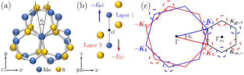
Figure 1: Schematic crystal structure of twisted bilayer MoS₂ with (a) top view and (b) side view. Electrons in different layers experience opposite effective electric fields due to local lack of mirror symmetry. (c) Moiré Brillouin zone(MBZ) formed by twisting hexagonal Brillouin zones of each layer. The in-plane spinor field exhibits opposite vorticities at $K_{m,+}$ and $K_{m,-}$ of MBZ due to layer-dependent Rashba effects.

While flat bands from VB states have enjoyed wide interest, moiré physics arising from conduction band (CB) states in twisted TMDs remains largely unexplored. One possible complication lies in the relatively weak SOC in the conduction bands on the scale of a few to tens of meVs GuiBin ; Rossier , which may cause crossings between spin-up and spin-down moiré bands. Recent works on untwisted TMDs, on the other hand, revealed that the small spin-orbit splitting in CB states, when combined with Rashba SOC introduced by mirror symmetry breaking, can lead to nontrivial Berry phase effects Benjamin ; Taguchi ; Lee . Notably, upon assembling two identical TMD layers into a twisted bilayer, the mirror symmetry is broken locally in each layer (Fig.1(a)-(b)) and Rashba SOC is expected to arise. How this SOC would affect the band topology of twisted TMDs is an outstanding question.

In this Letter we establish a novel topological phase generated by SOC in CB moiré bands in twisted TMDs, which is essentially different from those in twisted graphene Jianpeng1 ; Song ; Zaletel ; Senthil1 ; Senthil2 ; Wenyu where SOC is negligible, and those in the VB moiré bands of twisted TMDs where SOC plays no essential role in creating nonzero Chern numbers Wu2 . Focusing on the specific case of a twisted homobilayer MoS₂ we predict that an interplay among angular twist, local symmetry breaking and spin-orbit coupling in the CB states creates moiré flat bands with nonzero Chern numbers $\mathcal{C}=\pm 2$, and density-density interactions generically drive the system at $1/2$-filling into a valley-polarized correlated QAH state. We further show that the Chern bands generated by SOC stay robust against displacement fields which would otherwise destroy the nontrivial topology from layer-pseudospins Wu2 .

Continuum model for twisted homobilayer MoS₂.— Stacking two monolayers of MoS₂ with a small relative twist angle $\theta_{0}$ results in a moiré superlattice with lattice constant $a_{M}=a/\theta_{0}$, where $a$ is the lattice constant of each monolayer. The system has a symmetry group of $D_{3}\otimes\{U_{v}(1),\mathcal{T}\}$, where $U_{v}(1)$ stands for valley conservation, $\mathcal{T}$ for time-reversal symmetry, and the point group $D_{3}$ is generated by the three-fold rotation about the $z$-axis ($C_{3z}$) and a two-fold rotation about the $y$-axis ($C_{2y}$) (Fig.1(a)). For an aligned bilayer at $\theta_{0}=0$, the mirror symmetry $\mathcal{M}_{z}$ about the horizontal 2D mirror plane, which is respected in a monolayer, is broken locally on each layer. This generates uniform electric fields of opposite signs in different layers, which remain effective upon a small angular twist with $\theta_{0}\sim 1^{\circ}$ (Fig.1(b)). Based on models of monolayer MoS₂ with broken $\mathcal{M}_{z}$ Benjamin ; Taguchi ; Lee , the effective Hamiltonian for CB minima at $\pm K$ valleys of two twisted isolated layers can be written as:

$$\mathcal{H}^{\xi}_{0,l} = \sum_{\bm{k},\alpha\beta}c^{\dagger}_{\bm{k},l,\alpha}h^{\xi}_{l,\alpha\beta}(\bm{k})c_{\bm{k},l,\beta},$$ (1)

$$h^{\xi}_{l}(\bm{k}) = \frac{\hbar^{2}(\bm{k}-\xi\bm{K}_{l})^{2}}{2m^{\ast}}-\mu+\xi\beta_{\rm so}\sigma_{z}$$

$$+ (-1)^{l}\alpha_{\rm so}[(\bm{k}-\xi\bm{K}_{l})\times\bm{\sigma}]\cdot\hat{z},$$

where $\xi=\pm$ denotes the valley index, $l=1(2)$ labels the top (bottom) layer, $\alpha,\beta$ label the spin indices with the $\sigma$-matrices representing the usual Pauli matrices for spins. $\bm{K}_{1}\equiv\bm{K}_{m,+}$ and $\bm{K}_{2}\equiv\bm{K}_{m,-}$ are the shifted $+\bm{K}$-points on layer 1 and layer 2 (Fig.1(c)) due to the angular twist of $\theta_{0}$ equivalent to rotating the top (bottom) layer by an angle $\theta_{0}/2$ ($-\theta_{0}/2$) about the $z$-axis. In Eq.1, $m^{\ast}\approx 0.5m_{e}$ is the CB effective mass at $K$, $\mu$ is the Fermi energy measured from band minima. The $\alpha_{\rm so}$-term and $\beta_{\rm so}$-term account for the Rashba SOC and the Ising SOC, respectively. The Ising SOC has a valley-dependent sign due to time-reversal symmetry and causes a splitting of $\Delta_{\rm so}=2|\beta_{\rm so}|$ in the spin-up and spin-down CB states. The Rashba SOC has a layer-dependent sign imposed by $C_{2y}$ which swaps the two layers. Spatial variations of $\alpha_{\rm so}$ are discussed in Supplemental Material (SM).

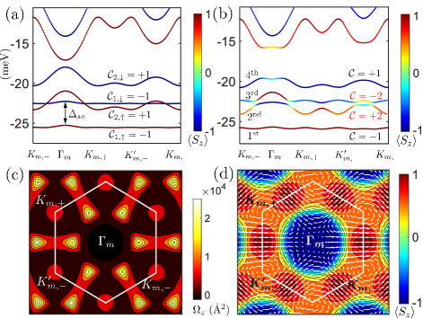
Figure 2: Moiré bands of valley $\xi=+$ formed by CB states of twisted homobilayer MoS₂ at $\theta_{0}=1.4^{\circ}$ with (a) $\alpha_{\rm so}=0$ and (b) $\alpha_{\rm so}\neq 0$. The colorbars indicate the out-of-plane spin expectation value $\braket{S_{z}}$ in units of $\hbar/2$. (c) Momentum-space profile of Berry curvature $\Omega_{z}$ in units of Ų in the 2${}^{\text{nd}}$ moiré band in (b). Large $\Omega_{z}$ of order 10⁴Ų emerges as a result of the nontrivial gap induced by SOC. (d) Momentum-space spin texture of the 2${}^{\text{nd}}$ moiré band in (b). White arrows indicate the in-plane spinor field, which has opposite vorticities at $K_{m,+}$ and $K_{m,-}$ and leads to a nontrivial skyrmion number $\mathcal{S}=+2$. Parameters used are presented in Table 1.

Spatial modulations due to the formation of moiré pattern can be captured by introducing coupling terms between states at $\bm{k}$ and $\bm{k}+\bm{G}_{M,j}$ Wu2 ; Senthil1 , where $\bm{G}_{M,j}=-\frac{4\pi}{\sqrt{3}a_{M}}(\cos\frac{(j-1)\pi}{3},\sin\frac{(j-1)\pi}{3})$ are the reciprocal vectors of the moiré superlattice. The momentum-space moiré potential is given by

$$\mathcal{H}_{M}=\sum_{\bm{k}}\sum_{j=1}^{6}\sum_{l=1,2}\sum_{\alpha=\uparrow,\downarrow}c^{\dagger}_{\bm{k},l,\alpha}V_{l,\bm{G}_{M,j}}c_{\bm{k}+\bm{G}_{M,j},l,\alpha},$$ (2)

where $V_{l,\bm{G}_{M,j}}=V_{M}(\cos\psi-i(-1)^{j}l\sin\psi)$ are complex coupling parameters with amplitude $V_{M}$ and phase $\psi$.

The effective inter-layer tunneling for states at $K$-valleys is modeled following the general recipe of two-center approximation MacDonald1 ; Wu2 , which can be written as

$$\mathcal{H}^{\xi}_{T}=-w_{0}\sum_{\bm{k}}c^{\dagger}_{\bm{k},1}(c_{\bm{k},2}+c_{\bm{k}+\xi\bm{G}_{M,2},2}+c_{\bm{k}+\xi\bm{G}_{M,3},2})+{\rm h.c.},$$ (3)

where $w_{0}$ denotes the effective inter-layer tunneling amplitude near $K$, which is extrapolated to be $w_{0}\approx 10$ meV using a combined approach of empirical models and Slater-Koster methods (see the Supplemental Material SM for details). The total non-interacting continuum model thus reads: $\mathcal{H}_{0}=\sum_{\xi=\pm}\sum_{l=1,2}\mathcal{H}^{\xi}_{0,l}+\mathcal{H}^{\xi}_{T}+\mathcal{H}_{M}$ with parameters tabulated in Table 1.

Moiré flat Chern bands and skyrmionic spin textures.— From general considerations, level spacings among the lowest moiré bands correspond roughly to the quantization energy $\Delta E\sim\hbar^{2}\pi^{2}/(2m^{*}a_{M}^{2})$ of an electron confined in a superlattice cell with size $a_{M}^{2}=a^{2}/\theta^{2}_{0}$. For $\theta_{0}\sim 1^{\circ}-2^{\circ}$, $\Delta E\sim 1-10$ meV in twisted MoS₂, which is comparable to the spin-orbit splitting $\Delta_{\rm so}\equiv 2|\beta_{\rm so}|=3$ meV caused by the Ising SOC GuiBin . If spin is conserved (e.g., in the absence of Rashba SOC), spin-up and spin-down moiré bands are expected to cross in general.

By setting $\alpha_{\rm so}=0$ in $\mathcal{H}_{0}$, we find that for $\xi=+$, the 1${}^{\text{st}}$ spin-down and the 2${}^{\text{nd}}$ spin-up moiré bands cross each other for $\theta_{0}\in(1.25^{\circ},1.5^{\circ})$. As a specific example, spin-resolved moiré bands at $\theta_{0}=1.4^{\circ}$ with $\alpha_{\rm so}=0$ are shown in Fig.2(a). With spin conservation in this case, the spin Chern number is well-defined, and the spin-up and spin-down bands involved in the level crossing have Chern numbers ($\mathcal{C}_{1,\downarrow}=+1$, $\mathcal{C}_{2,\uparrow}=-1$), which originate from the layer-pseudospin magnetic fields as in moiré bands from VB states Wu2 . Upon turning on $\alpha_{\rm so}$, crossing points are gapped out by the layer-dependent Rashba SOC which mix the spin-up and spin-down species (Fig.2(b)). As a result of this mixing, the original $\mathcal{C}_{1,\downarrow}$ and $\mathcal{C}_{2,\uparrow}$ from layer pseudospins annihilate each other; meanwhile, a new pair of flat bands (2${}^{\text{nd}}$ and 3${}^{\text{rd}}$ bands in Fig.2(b)) with Chern numbers $\mathcal{C}=\pm 2$ emerge (see SM SM for details on Chern number calculations). The nontrivial gap induced by Rashba SOCs is further signified by giant Berry curvatures of order $10^{4}$Ų in the MBZ (Fig.2(c)).

The unusual Chern numbers $\mathcal{C}=\pm 2$ arise from a unique combination of angular twist and local mirror-symmetry breaking: as moiré bands at opposite $\bm{K}_{m,+}$ and $\bm{K}_{m,-}$ points originate from states in different layers (Fig.1(c)), the layer-dependent Rashba SOCs (Eq.1) create an in-plane spinor field with opposite vorticities at $\bm{K}_{m,+}$ and $\bm{K}_{m,-}$ in the MBZ. This unsual pattern causes the in-plane spin to wind twice as one goes around a loop enclosing the $\Gamma_{m}$-point in the MBZ (Fig.2(d)). As we confirm numerically, the spin textures of the 2${}^{\textrm{nd}}$ and 3${}^{\textrm{rd}}$ moiré bands are characterized by nonzero skyrmion numbers $\mathcal{S}=\int d^{2}\bm{k}\hat{n}_{\bm{k}}\cdot(\partial_{k_{x}}\hat{n}_{\bm{k}}\times\partial_{k_{y}}\hat{n}_{\bm{k}})/4\pi=\pm 2$ ($\hat{n}_{\bm{k}}$: spin orientation of state at $\bm{k}$), and these two bands describe a two-level system with one-to-one correspondence between Chern numbers $\mathcal{C}$ and skyrmion number $\mathcal{S}$ Bernevig .

Table 1: Parameters used in $\mathcal{H}_{0}$ for twisted homobilayer MoS₂ with monolayer lattice constant $a=3.16{\AA}$.

$\mu$	$\alpha_{\rm so}$	$\beta_{\rm so}$	$V_{M}$	$\psi$	$w_{0}$
0 meV	80 meV$\cdot{\AA}$	-1.5 meV	10 meV	-89.6∘	10 meV

Correlated QAH state at $1/2$-filling.— Given the narrow bandwidth $W\approx 1$ meV of moiré Chern bands (Fig.2(b)), the characteristic Coulomb energy scale $g_{C}\simeq e^{2}/\epsilon a_{M}\approx 10$ meV overwhelms the kinetic energy and correlation physics is expected to arise (assuming $\theta_{0}=1.4^{\circ}$ and dielectric constant $\epsilon=10$ Bi ). Motivated by the observation that twisted graphene at $3/4-$filling can behave as an SU(4)-quantum Hall ferromagnet Senthil1 ; Sharpe ; Young ; Yazdani2 , and the fact that all CB moiré bands in Fig.2(b) involves only a two-fold valley degeneracy (note that spin SU(2)-symmetry is already broken by SOC), we examine correlation effects when the 2${}^{\text{nd}}$ moiré band is half-filled. For simplicity, we drop the band index $n$ in the following.

Including density-density interactions, the low-energy effective Hamiltonian: $\mathcal{H}_{\rm eff}=\mathcal{H}_{0,\rm eff}+\mathcal{H}_{I,\rm eff}$, where $\mathcal{H}_{0,\rm eff}=\sum_{\bm{k},\xi=\pm}E_{\xi}(\bm{k})c^{\dagger}_{\xi}(\bm{k})c_{\xi}(\bm{k})$ is the non-interacting part with band energies $E_{\xi}(\bm{k})$, and the interacting Hamiltonian compatible with $U_{v}(1)$ and $\mathcal{T}$ reads

$$\mathcal{H}_{I,\rm eff} = \sum_{\bm{k}\bm{k}^{\prime}\bm{q},\xi\xi^{\prime}}\frac{V(\bm{q})}{A}\Lambda^{\xi}(\bm{k}+\bm{q},\bm{k})\Lambda^{\xi^{\prime}}(\bm{k}^{\prime}-\bm{q},\bm{k}^{\prime})$$

$$\times c^{\dagger}_{\xi}(\bm{k}+\bm{q})c^{\dagger}_{\xi^{\prime}}(\bm{k}^{\prime}-\bm{q})c_{\xi^{\prime}}(\bm{k}^{\prime})c_{\xi}(\bm{k}),$$

where $V(\bm{q})$ is the Fourier transform of the two-body interaction, $A$ is the total area of the system, and $\Lambda^{\xi}(\bm{k}+\bm{q},\bm{k})\equiv\braket{u_{\xi,\bm{k}+\bm{q}}}{u_{\xi,\bm{k}}}$ ($\ket{u_{\xi,\bm{k}}}$: periodic part of the Bloch states) are the form factors arising from projecting the density-density interaction to active bands. The general trial Hartree-Fock ground state at $1/2$-filling has the form: $\ket{\Phi}=\prod_{\bm{k}\in\text{MBZ}}[w_{+}(\bm{k})c^{\dagger}_{+}(\bm{k})+w_{-}(\bm{k})c^{\dagger}_{-}(\bm{k})]\ket{\Phi_{0}}$, where $\ket{\Phi_{0}}$ is the vaccuum state with all lower-lying bands filled, and $w_{\xi}(\bm{k})$ are the variational parameters.

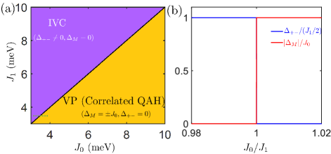
Figure 3: (a) $J_{0}-J_{1}$ phase diagram of the system with the 2${}^{\text{nd}}$ moiré band at $1/2$-filling. Under repulsive density-density interactions, only the $J_{1}\leq J_{0}$ regime can be accessed SM , where the valley-polarized(VP) state is generically favored and the system becomes a correlated QAH insulator. (b) Evolutions of the order parameters $\Delta_{+-}$ and $\Delta_{M}\equiv\Delta_{+}-\Delta_{-}$ as the ratio $J_{0}/J_{1}$ is tuned along the line-cut (green dashed line in (a)) across the phase boundary. A first-order transition happens at the critical point $J_{0}\simeq J_{1}$.

Minimizing $E^{\Phi}\equiv\braket{\Phi}{\mathcal{H}_{\rm eff}}{\Phi}$ with mean-field approximations for Fock exchange terms (see SM SM ) leads to a set of self-consistent equations:

$$\begin{cases}\Delta_{+}+\Delta_{-}=J_{0},\\ \Delta_{+}-\Delta_{-}=\frac{J_{0}}{2N}\sum_{\bm{k}}\frac{(\Delta_{+}-\Delta_{-})-\delta(\bm{k})}{D(\bm{k})},\\ \Delta_{+-}=\frac{J_{1}}{2N}\sum_{\bm{k}}\frac{\Delta_{+-}}{D(\bm{k})}.\end{cases}$$ (5)

Here, $J_{0}$ and $J_{1}$ denote the mean-field intra-valley and inter-valley exchange coupling constants, $\Delta_{\xi}=J_{0}\bar{n}_{\xi}$ ($\bar{n}_{\xi}$: mean occupancy for valley $\xi$) and $\Delta_{+-}$ are the intra-valley and inter-valley order parameters, which characterize the average energy gains from intra-valley and inter-valley exchange interactions, respectively. $\delta(\bm{k})\equiv E_{+}(\bm{k})-E_{-}(\bm{k})$ denotes energy difference between bands from two valleys $\xi=\pm$, $D(\bm{k})=\sqrt{\Delta^{2}_{+-}+[\delta(\bm{k})-\Delta_{M}]^{2}/4}$, where we introduce the valley magnetic order $\Delta_{M}\equiv\Delta_{+}-\Delta_{-}=J_{0}(\bar{n}_{+}-\bar{n}_{-})$.

Solutions of Eq.S27 are divided into two classes: (i) the valley-polarized (VP) state Adrian1 ; Senthil1 , in which one out of the two nearly degenerate moiré bands from two valleys is fully filled, with spontaneous $\mathcal{T}$-symmetry breaking: $\Delta_{M}=\xi J_{0},\Delta_{+-}=0,w_{\xi}(\bm{k})=1$; (ii) the inter-valley coherent (IVC) state, in which the Slater determinant is formed by coherent superpositions of states from the two valleys, with spontaneous U${}_{v}(1)$-symmetry breaking Adrian1 ; Senthil1 ; Senthil2 : $\Delta_{M}=0,\Delta_{+-}\approx J_{1}/2$, $w_{+,-}(\bm{k})\neq 0$. By comparing the energies of the VP and IVC states, we obtain the mean-field $J_{0}-J_{1}$ phase diagram for the range $0.3g_{C}\leq J_{0},J_{1}\leq g_{C}$ (Fig.3(a)). The IVC state is favored throughout the entire $J_{1}\geq J_{0}$ regime, while the VP phase takes up most of the $J_{1}<J_{0}$ regime. By tuning $J_{0}/J_{1}$ across the phase boundary (green dashed line in Fig.3(a)), a first-order transition occurs at $J_{0}\simeq J_{1}$ (Fig.3(b)).

It is worth noting that given a general repulsive interaction $V(\bm{q})>0$, the inequality $2|\Lambda^{+}(\bm{k}^{\prime},\bm{k})||\Lambda^{-}(\bm{k},\bm{k}^{\prime})|\leq|\Lambda^{+}(\bm{k}^{\prime},\bm{k})|^{2}+|\Lambda^{-}(\bm{k},\bm{k}^{\prime})|^{2}$ together with $\mathcal{T}$-symmetry leads to $J_{0}\geq J_{1}$, regardless of details of the form factors and the microscopic interaction SM . Thus, electron correlations most likely drive the system at $1/2$-filling into a $\mathcal{T}$-broken VP state, which realizes a correlated QAH state with $\mathcal{C}=\pm 2$. The case of general filling away from 1/2 is discussed in SM SM .

Effects of displacement fields and comparison with Chern bands from layer pseudospins.— As shown in Fig.2(a), with $\alpha_{\rm so}=0$, nonzero Chern numbers also arise in CB moiré bands due to layer pseudospin magnetic fields, with the same origin as those in VB moiré bands Wu2 . Thus, two different mechanisms for moiré Chern bands, one from layer pseudospin and the other from SOCs, coexist in the CB moiré bands. In contrast, the Rashba SOC is unimportant in the VB moiré bands where spin-up and spin-down bands are separated by $100-400$ meV GuiBin , and the VB moiré band topology is governed by layer pseudospin alone.

The nontrivial topology from layer pseudopsin is shown to be prone to displacement fields which can destroy the skyrmionic pseudospin textures by polarizing the layer-pseudospins Wu2 . On the other hand, the SOC mechanism has an independent origin in the avoided level crossings between spin-up and spin-down bands and does not require nontrivial layer pseudospin textures. Thus one would expect the nontrivial band topology in the CB moiré bands to be more robust against displacement fields than its VB counterpart.

To demonstrate the effects of displacement fields, we follow Refs.Wu2 and introduce a layer-dependent potential $V_{D,l}=(-1)^{l}V_{z}/2,(l=1,2)$ in $\mathcal{H}_{0}$. The moiré bands at $\theta_{0}=1.4^{\circ}$ under finite $V_{z}$ are shown in Fig.4(a), where we set $V_{z}=4$ meV strong enough to destroy the nontrivial topology generated by layer pseudospins (Fig.4(b)). Clearly, the avoided level crossings still occur and a pair of Chern bands with Chern numbers $(+1,-1)$ remain. The Chern number is reduced from $\mathcal{C}=\pm 2$ to $\mathcal{C}=\pm 1$ under $V_{z}$ because the displacement field drives a band inversion near $\bm{K}_{m,+}$ and mediates a Chern number exchange $\Delta\mathcal{C}=\pm 1$ between the 1${}^{\text{st}}$ and 2${}^{\text{nd}}$ moiré bands.

The topological phase diagram for CB moiré bands as a function of $\theta_{0}$ and $V_{z}$ is shown in Fig.4(b). Due to the extra mechanism from SOCs, the critical displacement field for the nontrivial topological regime is enhanced to be $V^{c2}_{z}$, which is 2-4 times of the critical $V^{c1}_{z}$ (yellow dashed line) needed to destroy the layer pseudospin mechanism for $\theta_{0}\sim 1^{\circ}$ ($V^{c1}_{z}$ obtained by setting $\alpha_{\rm so}=0$ in $\mathcal{H}_{0}$). Importantly, there is a wide parameter regime in the phase diagram (depicted in orange) where the layer pseudospin mechanism proposed in Ref.Wu2 fails while the CB moiré bands remain topological, which confirms that the CB states are more robust than VB states against displacement fields.

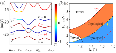
Figure 4: (a) CB Moiré bands for valley $\xi=+$ of twisted bilayer MoS₂ at $\theta_{0}=1.4^{\circ}$ and $V_{z}=4$ meV. Under finite $V_{z}$, spin-up and spin-down bands still cross, and the avoided level crossing due to SOC result in a pair of bands with $\mathcal{C}=\pm 1$. (b) Topological phase diagram of CB moiré bands as a function of $\theta_{0}$ and $V_{z}$, with an upper boundary $V_{z}^{c2}$ of the entire topological regime. Yellow dashed line: critical $V_{z}^{c1}$ above which nontrivial topology generated by layer-pseudospin is destroyed. Values of $V^{c1}_{z}$ are similar to those found in VB moiré bands Wu2 . Area enclosed by the red dashed lines: regime with level crossings between spin-up and spin-down CB moiré bands when $\alpha_{\rm so}=0$. Area in orange: topological regime where layer pseudospin mechanism in Ref.Wu2 fails.

Conclusion and Discussions. — While on-going activities in twisted TMDs have focused mainly on VB moiré bands Wu2 ; Wu3 ; LeRoy ; Fai1 ; Wang ; Dean ; Bi , our proposal of moiré Chern bands generated by SOC opens a new pathway into the largely unknown territory of CB moiré physics. When these Chern bands are half-filled, according to our predictions, electron interactions can lead to a spontaneously $\mathcal{T}$-broken VP phase and realize a correlated QAH state, which will manifest itself through quantized Hall conductance in transport measurements.

To realize the topological moiré bands generated by SOC, any finite Rashba SOC which is allowed by the $D_{3}$-symmetry of the system would be sufficient, in principle, to induce a nontrivial gap. Notably, as MoS₂ is intrinsically semiconducting (with Fermi level $\sim 0.8$ eV below the conduction band edge) Xiao ; GuiBin ; Fai2 , it is necessary to gate the chemical potential such that the CB moiré bands are filled in the first place. With the dual-gate setup used widely in experiments Cao1 ; Dean , local mirror symmetry breaking can be further enhanced by interfacial contact with gating electrodes, which enhances the SOC gap in the non-interacting bands. Due to the correlated nature of the QAH state at 1/2-filling, the actual topological gap to be manifested experimentally is not solely determined by the SOC gap in the non-interacting bands; instead it should be largely governed by the intra-valley exchange coupling $J_{0}\sim 10$ meV for $\theta_{0}\sim 1^{\circ}$ SM . This sizable correlation-induced topological gap will reduce complications of disorder and thermal effects in experimental detection of the predicted correlated QAH state. However, as $\theta_{0}$ increases, correlation effects become weaker and the moiré bands more dispersive, thus the predicted correlated QAH phase would be less robust in the large twist angle regime.

Acknowledgement. — B.T.Z. thanks Zefei Wu and Ziliang Ye for inspiring discussions on experimental aspects of twisted MoS₂. This work was supported by NSERC and the Canada First Research Excellence Fund, Quantum Materials and Future Technologies Program. B.T.Z. further acknowledges the support of the Croucher Foundation.

I. Calculation of effective inter-layer tunneling parameter $w_{0}$

In the main text, we mention that an effective inter-layer tunneling parameter $w_{0}$ is extrapolated using a combined approach of empirical model and Slater-Koster method. Here, we present details on the calculation of $w_{0}$.

The inter-layer tunneling between two MoS₂ monolayers with a small twist angle can be conveniently modeled by the two-center approximation following the general recipe introduced in previous studies on twisted bilayer graphene MacDonaldS and twisted homobilayer MoTe₂ WuS . Particularly, electronic states near the conduction band minimum of monolayer transition-metal dichalcogenides(TMDs) are predominantly from the $4d_{z^{2}}$-orbitals of the transition metal atoms GuiBinS and the inter-layer tunneling is expected to be mediated by the $\sigma$-bonding between $4d_{z^{2}}$-orbitals in each layer. To start with, we consider fermionic operators that create Bloch states of the form:

$$c^{\dagger}_{\bm{k},1,\alpha} = \frac{1}{\sqrt{N}}\sum_{\bm{R}}e^{i\bm{k}\cdot\bm{R}}c^{\dagger}_{1,\alpha}(\bm{R}),$$ (S1)

$$c^{\dagger}_{\bm{k}^{\prime},2,\beta} = \frac{1}{\sqrt{N}}\sum_{\bm{R}^{\prime}}e^{i\bm{k}^{\prime}\cdot(\bm{R}^{\prime}+\bm{d}_{0})}c^{\dagger}_{2,\beta}(\bm{R}^{\prime}+\bm{d}_{0}).$$

Here, $\bm{k},\bm{R}$ and $\bm{k}^{\prime},\bm{R}^{\prime}$ denote the momentum and lattice vectors of layer 1 and 2, respectively. $c^{\dagger}_{l,\alpha}(\bm{R})$ creates a localized Wannier orbital of $d_{z^{2}}$ character with spin $\alpha$ at site $\bm{R}$ in layer $l$. In general, the inter-layer tunneling Hamiltonian is given by:

$$\mathcal{H}_{T}=\sum_{\bm{k},\bm{k}^{\prime}}\sum_{\alpha,\beta}c^{\dagger}_{\bm{k},1,\alpha}T_{\alpha\beta}(\bm{k},\bm{k}^{\prime})c_{\bm{k}^{\prime},2,\beta}+h.c.$$ (S2)

where the tunneling matrix $T$ reads:

$$T_{\alpha\beta}(\bm{k},\bm{k}^{\prime}) = \braket{\bm{k},1,\alpha}{\mathcal{H}_{T}}{\bm{k}^{\prime},2,\beta}$$

$$= \frac{1}{N}\sum_{\bm{R},\bm{R}^{\prime}}e^{-i\bm{k}\cdot\bm{R}}e^{i\bm{k}^{\prime}\cdot(\bm{R}^{\prime}+\bm{d}_{0})}\braket{\bm{R},1,\alpha}{\mathcal{H}_{T}}{\bm{R}^{\prime}+\bm{d}_{0},2,\beta}$$

$$(\text{two-center approximation) } = -\frac{1}{N}\sum_{\bm{R},\bm{R}^{\prime}}e^{-i\bm{k}\cdot\bm{R}}e^{i\bm{k}^{\prime}\cdot(\bm{R}^{\prime}+\bm{d}_{0})}t_{\alpha\beta}(\bm{R}-\bm{R}^{\prime}-\bm{d}_{0})$$

$$= -\frac{1}{N}\sum_{\bm{R},\bm{R}^{\prime},\bm{q}}e^{-i\bm{k}\cdot\bm{R}}e^{i\bm{k}^{\prime}\cdot(\bm{R}^{\prime}+\bm{d}_{0})}\frac{t_{\alpha\beta}(\bm{q})}{A}e^{i\bm{q}\cdot(\bm{R}-\bm{R}^{\prime}-\bm{d}_{0})}$$

$$= -\frac{1}{N}\sum_{\bm{q}}\frac{t_{\alpha\beta}(\bm{q})}{A}e^{i(\bm{k}^{\prime}-\bm{q})\cdot\bm{d}_{0}}\big{(}\sum_{\bm{R}}e^{i(\bm{q}-\bm{k})\cdot\bm{R}}\big{)}\big{(}\sum_{\bm{R}^{\prime}}e^{i(\bm{k}^{\prime}-\bm{q})\cdot\bm{R}^{\prime}}\big{)}$$

$$= -\sum_{\bm{G},\bm{G}^{\prime}}\frac{t_{\alpha\beta}(\bm{k}+\bm{G})}{\Omega}e^{-i\bm{G}^{\prime}\cdot\bm{d}_{0}}\delta_{\bm{k}+\bm{G},\bm{k}^{\prime}+\bm{G}^{\prime}}$$

Here, $t_{\alpha\beta}(\bm{q})=\int d^{2}\bm{r}t_{\alpha\beta}(\bm{r})e^{-i\bm{q}\cdot\bm{r}}$ is the Fourier transform of $t_{\alpha\beta}(\bm{r})$, $A$ is the total area of the system, $\Omega=A/N$ is the area of the primitive unit cell. In the last step of the derivation above, we made use of the identity $\sum_{\bm{R}}e^{i(\bm{q}-\bm{k})\cdot\bm{R}}=N\sum_{\bm{G}}\delta_{\bm{q},\bm{k}+\bm{G}}$.

To simplify the expression of $T_{\alpha\beta}(\bm{k},\bm{k}^{\prime})$ above, we note that for the relevant electronic states near the $K$-points with $\bm{k}\sim\xi\bm{K}$, the dominant $t_{\alpha\beta}(\bm{q})$-terms that enter the continuum model for valley $\xi$ involve only 3 different reciprocal lattice vectors $\bm{G}=\bm{0},\xi\bm{G}_{2},\xi\bm{G}_{3}$ for the top layer ($\bm{G}^{\prime}=\bm{0},\xi\bm{G}^{\prime}_{2},\xi\bm{G}^{\prime}_{3}$ accordingly for the bottom layer). Thus, the effective inter-layer tunneling Hamiltonian can be written as:

$$\mathcal{H}^{\xi}_{T,eff} = -\frac{1}{\Omega}\sum_{\bm{k}}\sum_{\alpha,\beta}c^{\dagger}_{\bm{k},1,\alpha}t_{\alpha\beta}(\xi\bm{K})c_{\bm{k},2,\beta}+c^{\dagger}_{\bm{k},1,\alpha}t_{\alpha\beta}(\xi\bm{K}+\xi\bm{G}_{2})e^{-i\xi\bm{G}^{\prime}_{2}\cdot\bm{d}_{0}}c_{\bm{k}+\xi\bm{G}_{M,2},2,\beta}$$

$$+ c^{\dagger}_{\bm{k},1,\alpha}t_{\alpha\beta}(\xi\bm{K}+\xi\bm{G}_{3})e^{-i\xi\bm{G}^{\prime}_{3}\cdot\bm{d}_{0}}c_{\bm{k}+\xi\bm{G}_{M,3},2,\beta}+h.c.$$

$$= -\sum_{\bm{k},\alpha\beta}c^{\dagger}_{\bm{k},1,\alpha}w_{\alpha\beta}c_{\bm{k},2,\beta}+c^{\dagger}_{\bm{k},1,\alpha}w_{\alpha\beta}e^{-i\xi\bm{G}^{\prime}_{2}\cdot\bm{d}_{0}}c_{\bm{k}+\xi\bm{G}_{M,2},2,\beta}$$

$$+ c^{\dagger}_{\bm{k},1,\alpha}w_{\alpha\beta}e^{-i\xi\bm{G}^{\prime}_{3}\cdot\bm{d}_{0}}c_{\bm{k}+\xi\bm{G}_{M,3},2,\beta}+h.c.,$$

where $w_{\alpha\beta}=t_{\alpha\beta}(K)/\Omega$, $\bm{G}_{M,j}=\bm{G}_{j}-\bm{G}^{\prime}_{j}$. Explicitly, the tunneling matrices connecting states at $\bm{k}$ on layer 1 to those at $\bm{k},\bm{k}+\xi\bm{G}_{M,2},\bm{k}+\xi\bm{G}_{M,3}$ on layer 2 are listed below:

$$T_{\alpha\beta}(\bm{k},\bm{k})=-w_{\alpha\beta},T_{\alpha\beta}(\bm{k},\bm{k}+\xi\bm{G}_{M,2})=-e^{-i\xi\bm{G}^{\prime}_{2}\cdot\bm{d}_{0}}w_{\alpha\beta},T_{\alpha\beta}(\bm{k},\bm{k}+\xi\bm{G}_{M,3})=-e^{-i\xi\bm{G}^{\prime}_{3}\cdot\bm{d}_{0}}w_{\alpha\beta}.$$ (S5)

For simplicity, we consider the case with $\bm{d}_{0}=\bm{0}$ where metal sites from the two layers are aligned at zero twist angle, and assume $w_{\alpha\beta}=w\delta_{\alpha\beta}$ given that the inter-layer tunneling is usually dominated by spin-preserving processes. This leads to the form of the inter-layer tunneling Hamiltonian in Eq.3 of the main text.

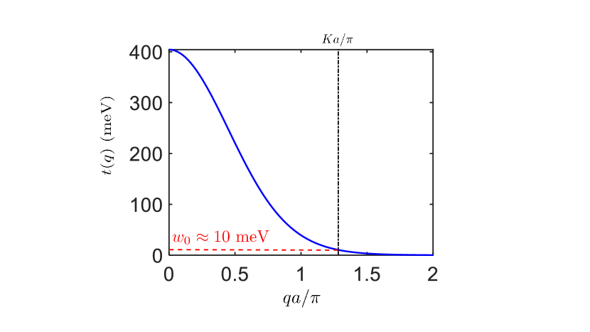
Figure S1: Interlayer tunneling strength $t(q)$ as a function of $q$ calculated by numerical Fourier transform. Dashed vertical line in black indicates the value $w\approx 10$ meV extrapolated at $q=K$ where $Ka/\pi=4/3$.

To evaluate the effective tunneling strength $t(\bm{q}=\bm{K})$ near the $\bm{K}$-points, we use the following simple model for $t(\bm{r})$ which incorporates the Slater-Koster $\sigma$-bonding between $d_{z^{2}}$-orbitals in the two different layers with an empirical exponential decay:

$$t(\bm{r}) = [n^{2}(\bm{r})-(l^{2}(\bm{r})+m^{2}(\bm{r}))/2]^{2}V_{dd\sigma}(\bm{r}),$$ (S6)

$$V_{dd\sigma}(\bm{r}) = t_{0}e^{-\lambda\sqrt{d^{2}+|\bm{r}|^{2}}}.$$

Here, $d=0.7$ nm is the inter-layer distance between two TMD monolayers SunS , $n(\bm{r}),l(\bm{r}),m(\bm{r})$ are the directional cosines of the vector $\bm{r}$ connecting the two position vectors in the two layers, with

$$n^{2}(\bm{r})=\frac{d^{2}}{d^{2}+|\bm{r}|^{2}},\hskip 28.45274ptl^{2}(\bm{r})+m^{2}(\bm{r})=\frac{|\bm{r}|^{2}}{d^{2}+|\bm{r}|^{2}}.$$ (S7)

The value of $\lambda$ is estimated based on the empirical fact that $t^{\prime}\approx 0.1t$, where $t^{\prime}$ and $t$ are the next-nearest-neighbor and neareast-neighbor hopping amplitudes. Thus, $t/t^{\prime}=e^{\lambda a}\approx 10$, and $\lambda a=ln(10)\approx 2.3$. Note that the form of $t(\bm{r})$ in Eq.S6 is a radial function $t(\bm{r})\equiv t(r)$, and its Fourier transform has the general form of:

$$t(q) = \int_{0}^{\infty}drrt(r)\int_{0}^{2\pi}d\theta e^{-iqr\cos\theta}$$

$$= 2\pi\int_{0}^{\infty}drrJ_{0}(qr)t(r),$$

where $J_{0}(x)$ is the Bessel function of order zero. With the form of $t(r)$ in Eq.S6, $t(q)$ can be obtained by numerical integration with the only fitting parameter $t_{0}$. To fix $t_{0}$, we note that states near the $\Gamma$-point of the valence band states in MoS₂ also originate from $4d_{z^{2}}$-orbitals GuiBinS , and the inter-layer coupling causes an energy splitting of $\Delta E\simeq 2t(q=0)\approx 800$ meV at the $\Gamma$-point in the valence bands in aligned bilayer MoS₂ ZahidS . This implies $t(q=0)\approx 400$ meV and allows us to fix $t_{0}$ and obtain the values of $t(q)$ for all $q$ as shown in Fig.S1. The effective interlayer coupling strength at the $K$-point in our continuum model is then extrapolated to be $w_{0}\approx 10$ meV at $qa=Ka=4\pi/3$ (dashed vertical line in black in Fig.S1).

II. Chern numbers in moiré bands

A. Numerical method for computing Chern numbers

The Chern numbers of the CB moiré bands presented in Fig.2 and Fig.4 of the main text are calculated numerically using the standard formula introduced in Ref.SuzukiS . The procedures of the numerical method is outlined below. For the sake of simplicity, we consider a given CB moiré band and drop the band index in the following.

First, we construct a discretized moiré Brillouin zone (MBZ) with an $N_{x}\times N_{y}$ grid. For each momentum point $\bm{k}$ in the grid, we evaluate the following complex quantities:

$$U_{x}(\bm{k}) \equiv \braket{u(\bm{k}+\Delta k_{x}\hat{x})}{u(\bm{k})},$$ (S9)

$$U_{y}(\bm{k}) \equiv \braket{u(\bm{k}+\Delta k_{y}\hat{y})}{u(\bm{k})},$$

where $\ket{u(\bm{k})}$ is the periodic part of the Bloch state at $\bm{k}$, $\hat{x},\hat{y}$ are unit vectors in $k_{x}$ and $k_{y}$ directions, $\Delta k_{x}$ and $\Delta k_{y}$ measure the spacings between neighboring grid points in $k_{x}$ and $k_{y}$ directions. Note that the phase factors of $U_{x}$ and $U_{y}$ essentially account for the Berry connections on each link between two neighboring grid points. The gauge-invariant Berry flux threading through one plaquette around $\bm{k}$ is given by $\gamma_{\bm{k}}=\arg W(\bm{k})$, where $W(\bm{k})$ is the Wilson loop:

$$W(\bm{k})=U_{x}(\bm{k})U_{y}(\bm{k}+\Delta k_{x}\hat{x})U^{\ast}_{x}(\bm{k}+\Delta k_{y}\hat{y})U^{\ast}_{y}(\bm{k}).$$ (S10)

The Chern number is then expressed as the sum over all Berry fluxes $\gamma_{\bm{k}}$ through a total number of $N_{x}\times N_{y}$ plaquettes:

$$\mathcal{C}=\frac{1}{2\pi}\sum_{\bm{k}}\gamma_{\bm{k}}.$$ (S11)

We note that to obtain accurate results for Chern numbers in the continuum model, the total number of grid points must be large enough such that $|\arg W(\bm{k})|<\pi$ for all $\bm{k}$, and the total number $M$ of the moiré Brillouin zones must also be large enough to ensure an accurate description of the low-energy physics at the exact $M\rightarrow\infty$ limit. In our model, we find that $N_{x}=N_{y}=40$ and $M=81$ produce accurate numerical results for $\mathcal{C}$ in the CB moiré bands.

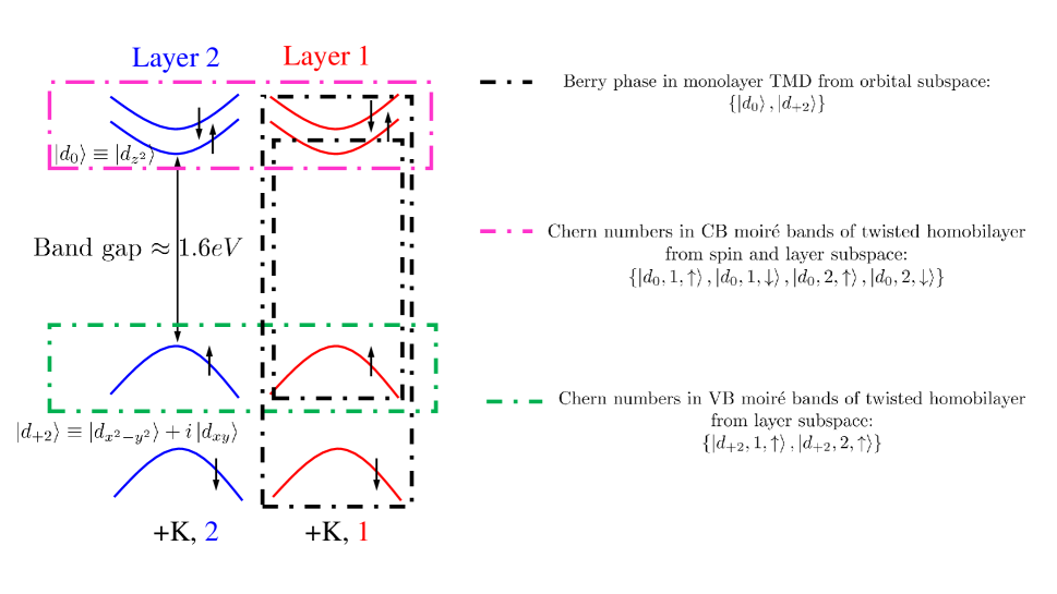
Figure S2: Different sets of degrees of freedom involved in (i) Berry phase in monolayer TMD (encircled by black dashed rectangles), (ii) Chern numbers in CB moiré bands (encircled by pink dashed rectangles), and (iii) Chern numbers in VB moiré bands (encircled by green dashed rectangles).

B. Effects of Berry phase in monolayer transition-metal dichalcogenides

It is known that a Berry phase with value close to $\pi$ can appear in a local region around $K$-points in the Brillouin zone of a monolayer transition-metal dichalcogenide (TMD) XiaoS . This Berry phase originates from the massive Dirac Hamiltonian involving both the conduction and valence band edges at $+K$-point (see black dashed rectangles in Fig.S2), which is essentially different from both the Berry curvatures generated by the layer degrees of freedom in VB moiré bands WuS (green dashed rectangles in Fig.S2)) and the giant Berry curvatures (Fig.2(c) of the main text) generated by the spin and layer degrees of freedom in our continuum model (pink dashed rectangles in Fig.S2)).

While by summing over both the spin-up and spin-down valence bands in a monolayer TMD at one of the $K$-valleys, one acquires a total Berry phase close to $2\pi$ and appears to correspond to a “Chern number” of 1 for this valley, such a “Chern number” is, strictly speaking, not well-defined. This is because the Berry curvatures in a monolayer are summed over two bands and integrated only over a local region around $+K$ in the (large) monolayer Brillouin zone. The integral is not guaranteed to be quantized by any topological reasons. In contrast, the Chern numbers in both the CB moiré bands in the main text and the VB moiré bands in Ref.WuS are well-defined quantities because the Berry curvatures of each single band are integrated over the entire (small) moiré Brillouin zone. The resultant Chern numbers of each band from valley $\xi=+$ or $\xi=-$ are guaranteed to be quantized by topology.

Importantly, we note that the Berry phase in monolayer TMDs do not affect the topology of CB moiré bands in a twisted homobilayer. This is because the Berry curvatures from the massive Dirac Hamiltonian is only on the order of $\sim 10{\AA}^{2}$ XiaoS , three orders of magnitude smaller than the Berry curvatures $\sim 10^{4}{\AA}^{2}$ in the moiré Chern bands (Fig.2(c) of the main text) generated by spin and layer degrees of freedom. Thus, the topology of CB moiré bands is dictated by the spin and layer degrees of freedom, which justifies why the contributions from remote valence bands ($\sim$ 1.6 eV away from conduction band states) can be neglected.

III. Self-consistent Hartree-Fock calculations

A. Hartree-Fock energy functional and Lagrange equations

When the Chern bands in a twisted bilayer MoS₂ are half-filled, the low-energy effective Hamiltonian is written as:

$$\mathcal{H}_{eff}=\mathcal{H}_{0,eff}+\mathcal{H}_{I,eff}$$ (S12)

where the non-interacting Hamiltonian is given by

$$\mathcal{H}_{0,eff}=\sum_{\bm{k}}\sum_{\xi=\pm}E_{\xi}(\bm{k})c^{\dagger}_{\xi}(\bm{k})c_{\xi}(\bm{k})$$ (S13)

Here, $\xi=\pm$ is the valley index, $E_{\xi}(\bm{k})$ is the energy of moiré band from valley $\xi$. The effective interacting Hamiltonian is given by:

$$\mathcal{H}_{I,eff} = \sum_{\bm{k},\bm{k}^{\prime},\bm{q}}\frac{V(\bm{q})}{A}\sum_{\xi\xi^{\prime}}\Lambda^{\xi}(\bm{k}+\bm{q},\bm{k})\Lambda^{\xi^{\prime}}(\bm{k}^{\prime}-\bm{q},\bm{k}^{\prime})$$

$$\times c^{\dagger}_{\xi}(\bm{k}+\bm{q})c^{\dagger}_{\xi^{\prime}}(\bm{k}^{\prime}-\bm{q})c_{\xi^{\prime}}(\bm{k}^{\prime})c_{\xi}(\bm{k}),$$

where $V(\bm{q})=\int d^{2}\bm{r}V(\bm{r})e^{i\bm{q}\cdot\bm{r}}$ is the Fourier transform of the two-body interaction $V(\bm{r}_{1}-\bm{r}_{2})$, $A$ is the total area of the system, $\Lambda^{\xi}(\bm{k}+\bm{q},\bm{k})\equiv\braket{u_{\xi,\bm{k}+\bm{q}}}{u_{\xi,\bm{k}}}$ are the form factors arising from projecting the general density-density interaction to the active bands, which end up as the overlap between the cell-periodic parts of Bloch states within the same band from valley $\xi$. Note that due to the $U_{v}(1)$-symmetry, wave functions from different valleys do not overlap: $\Lambda^{+-}(\bm{k}^{\prime},\bm{k})\equiv\braket{u_{+,\bm{k}^{\prime}}}{u_{-,\bm{k}}}=0$.

As mentioned in the main text, the Coulomb energy scale $g_{C}\sim 10$ meV in twisted bilayer MoS₂ overhelms the band width $W\sim 1$ meV in the Chern bands found in the continuum model. This motivates us to consider possible ground states at $1/2$-filling as a general Hartree-Fock state of the form: $\ket{\Phi}=\prod_{\bm{k}}[w_{+}(\bm{k})e^{i\theta_{+}(\bm{k})}c^{\dagger}_{+}(\bm{k})+w_{-}(\bm{k})e^{i\theta_{-}(\bm{k})}c^{\dagger}_{-}(\bm{k})]\ket{\Phi_{0}}$, where $w_{\xi}(\bm{k})$ and $\theta_{\xi}(\bm{k})$ are real numbers and denote the amplitude and phase of the coefficients of valley $\xi$ at momentum $\bm{k}$. $\ket{\Phi_{0}}$ is the vaccuum state with all bands below the active bands being fully filled. The variational parameters can be determined by minimizing the ground state energy subject to the normalization condition $w^{2}_{+}(\bm{k})+w^{2}_{-}(\bm{k})=1$. The energy of $\ket{\Phi}$ is given by:

$$E^{\Phi}\equiv\braket{\Phi}{\mathcal{H}_{eff}}{\Phi}=E^{\Phi}_{0}+E_{H}+E^{\Phi}_{F},$$ (S15)

where $E^{\Phi}_{0}$, $E_{H}$ and $E^{\Phi}_{F}$ refer to the kinetic energy, Hartree energy, and the Fock exchange energy of $\ket{\Phi_{0}}$, respectively. It is straightforward to show that the Hartree term essentially accounts for the direct coupling: $E_{H}\propto n_{e}^{2}$, where $n_{e}$ is the electron density of the system, which is fixed at a given band filling. Thus, we neglect $E_{H}$ from now on and focus on $E^{\Phi}_{0}$ and $E^{\Phi}_{F}$:

$$E^{\Phi}_{0} = \sum_{\bm{k}}w^{2}_{+}(\bm{k})E_{+}(\bm{k})+w^{2}_{-}(\bm{k})E_{-}(\bm{k}),$$ (S16)

$$E^{\Phi}_{F} = -\sum_{\bm{k},\bm{q}}\frac{V(\bm{q})}{A}\sum_{\xi\xi^{\prime}}\Lambda^{\xi}(\bm{k}+\bm{q},\bm{k})\Lambda^{\xi^{\prime}}(\bm{k},\bm{k}+\bm{q})w_{\xi}(\bm{k}+\bm{q})w_{\xi^{\prime}}(\bm{k}+\bm{q})w_{\xi}(\bm{k})w_{\xi^{\prime}}(\bm{k})$$

$$\times e^{-i\theta_{\xi}(\bm{k}+\bm{q})}e^{i\theta_{\xi^{\prime}}(\bm{k}+\bm{q})}e^{-i\theta_{\xi^{\prime}}(\bm{k})}e^{i\theta_{\xi}(\bm{k})}.$$

Note that in order to minimize $E^{\Phi}_{F}$, the phase factors would adjust themselves such that $e^{-i\theta_{\xi}(\bm{k}+\bm{q})}e^{i\theta_{\xi}(\bm{k})}\Lambda^{\xi}(\bm{k}+\bm{q},\bm{k})=|\Lambda^{\xi}(\bm{k}+\bm{q},\bm{k})|$. This reduces $E^{\Phi}_{F}$ to the following form:

$$E^{\Phi}_{F}=-\sum_{\bm{k},\bm{q}}\frac{V(\bm{q})}{A}\sum_{\xi\xi^{\prime}}|\Lambda^{\xi}(\bm{k}+\bm{q},\bm{k})||\Lambda^{\xi^{\prime}}(\bm{k}+\bm{q},\bm{k})|w_{\xi}(\bm{k}+\bm{q})w_{\xi^{\prime}}(\bm{k}+\bm{q})w_{\xi}(\bm{k})w_{\xi^{\prime}}(\bm{k})$$ (S17)

where we have used the identity $|\Lambda^{\xi^{\prime}}(\bm{k},\bm{k}+\bm{q})|=|\Lambda^{\xi^{\prime}}(\bm{k}+\bm{q},\bm{k})^{\ast}|=|\Lambda^{\xi^{\prime}}(\bm{k}+\bm{q},\bm{k})|$. To minimize $E^{\Phi}_{0}+E^{\Phi}_{F}$ subject to the constraint $w^{2}_{+}(\bm{k})+w^{2}_{-}(\bm{k})=1$, we introduce the Langrange multipliers $\lambda_{\bm{k}}$ such that

$$\partial_{w_{\xi}(\bm{k})}\big{[}E^{\Phi}_{0}+E^{\Phi}_{F}-\sum_{\bm{k}}\lambda_{\bm{k}}(w^{2}_{+}(\bm{k})+w^{2}_{-}(\bm{k}))\big{]}=0.$$ (S18)

This leads to the following two equations:

$$\begin{cases}\big{[}E_{+}(\bm{k})-\sum_{\bm{q}}g_{+}(\bm{q},\bm{k})w^{2}_{+}(\bm{k}+\bm{q})]w_{+}(\bm{k})-[\sum_{\bm{q}}g_{+-}(\bm{q},\bm{k})w_{+}(\bm{k}+\bm{q}))w_{-}(\bm{k}+\bm{q})\big{]}w_{-}(\bm{k})=\lambda_{\bm{k}}w_{+}(\bm{k})\\ \big{[}E_{-}(\bm{k})-\sum_{\bm{q}}g_{-}(\bm{q},\bm{k})w^{2}_{-}(\bm{k}+\bm{q})]w_{-}(\bm{k})-[\sum_{\bm{q}}g_{+-}(\bm{q},\bm{k})w_{-}(\bm{k}+\bm{q})w_{-}(\bm{k}+\bm{q})\big{]}w_{+}(\bm{k})=\lambda_{\bm{k}}w_{-}(\bm{k})\end{cases}$$ (S19)

where we introduced the shorthand notation:

$$\begin{cases}g_{\xi}(\bm{q},\bm{k})=V(\bm{q})|\Lambda^{\xi}(\bm{k}+\bm{q},\bm{k})|^{2}/A,(\xi=\pm)\\ g_{+-}(\bm{q},\bm{k})=V(\bm{q})|\Lambda^{+}(\bm{k}+\bm{q},\bm{k})||\Lambda^{-}(\bm{k}+\bm{q},\bm{k})|/A.\end{cases}$$ (S20)

As we seek for nontrivial solutions of Eq.S19, it is convenient to introduce the following two quantities:

$$\Delta_{\xi}(\bm{k}) = \sum_{\bm{q}}g_{\xi}(\bm{q},\bm{k})w^{2}_{\xi}(\bm{k}+\bm{q}),$$ (S21)

$$\Delta_{+-}(\bm{k}) = \sum_{\bm{q}}g_{+-}(\bm{q},\bm{k})w_{+}(\bm{k}+\bm{q})w_{-}(\bm{k}+\bm{q}),$$

which allows us to reformulate Eq.S19 as an eigenvalue equation:

$$\begin{pmatrix}E_{+}(\bm{k})-\Delta_{+}(\bm{k})&-\Delta_{+-}(\bm{k})\\ -\Delta_{+-}(\bm{k})&E_{-}(\bm{k})-\Delta_{-}(\bm{k})\end{pmatrix}\begin{pmatrix}w_{+}(\bm{k})\\ w_{-}(\bm{k})\end{pmatrix}=\lambda_{\bm{k}}\begin{pmatrix}w_{+}(\bm{k})\\ w_{-}(\bm{k})\end{pmatrix}.$$ (S22)

Note that $\lambda_{\bm{k}}$ has the physical interpretation as the energy contribution from $\bm{k}$ to the total energy of the Hartree-Fock state. This motivates us to focus on the lower branch of eigenvalues of the $2\times 2$ symmetric matrix:

$$\lambda_{1}(\bm{k})=\frac{1}{2}[E_{+}(\bm{k})+E_{-}(\bm{k})-(\Delta_{+}(\bm{k})+\Delta_{-}(\bm{k}))]-\sqrt{\Delta^{2}_{+-}(\bm{k})+\frac{1}{4}[E_{+}(\bm{k})-E_{-}(\bm{k})-(\Delta_{+}(\bm{k})-\Delta_{-}(\bm{k}))]^{2}}$$ (S23)

with the corresponding eigenvector $[w_{+}(\bm{k}),w_{-}(\bm{k})]^{T}=[\cos(\phi_{\bm{k}}/2),\sin(\phi_{\bm{k}}/2)]^{T}$, where

$$\sin(\phi_{\bm{k}}) = \frac{\Delta_{+-}(\bm{k})}{\sqrt{\Delta^{2}_{+-}(\bm{k})+\frac{1}{4}[E_{+}(\bm{k})-E_{-}(\bm{k})-(\Delta_{+}(\bm{k})-\Delta_{-}(\bm{k}))]^{2}}}=2\cos(\phi_{\bm{k}}/2)\sin(\phi_{\bm{k}}/2),$$ (S24)

$$\cos(\phi_{\bm{k}}) = \frac{1}{2}\frac{(\Delta_{+}(\bm{k})-\Delta_{-}(\bm{k}))-(E_{+}(\bm{k})-E_{-}(\bm{k}))}{\sqrt{\Delta^{2}_{+-}(\bm{k})+\frac{1}{4}[E_{+}(\bm{k})-E_{-}(\bm{k})-(\Delta_{+}(\bm{k})-\Delta_{-}(\bm{k}))]^{2}}}=\cos^{2}(\phi_{\bm{k}}/2)-\sin^{2}(\phi_{\bm{k}}/2).$$

The defining equations (Eq.S21) require that $\Delta_{+}(\bm{k}),\Delta_{-}(\bm{k}),\Delta_{+-}(\bm{k})$ satisfy the following self-consistent equations:

$$\Delta_{+}(\bm{k}) = \frac{1}{N}\sum_{\bm{k}^{\prime}}J_{++}(\bm{k}^{\prime},\bm{k})\frac{1+\cos(\phi_{\bm{k}^{\prime}})}{2},$$ (S25)

$$\Delta_{-}(\bm{k}) = \frac{1}{N}\sum_{\bm{k}^{\prime}}J_{--}(\bm{k}^{\prime},\bm{k})\frac{1-\cos(\phi_{\bm{k}^{\prime}})}{2},$$

$$\Delta_{+-}(\bm{k}) = \frac{1}{N}\sum_{\bm{k}^{\prime}}J_{+-}(\bm{k}^{\prime},\bm{k})\frac{\sin(\phi_{\bm{k}^{\prime}})}{2}.$$

Here, $J_{\xi\xi^{\prime}}(\bm{k},\bm{k}^{\prime})$ are the Fock exchange functions:

$$J_{\xi\xi^{\prime}}(\bm{k}^{\prime},\bm{k})=\Omega^{-1}\sum_{\bm{G}_{M}}V(\bm{k}^{\prime}+\bm{G}_{M}-\bm{k})|\Lambda^{\xi}(\bm{k}^{\prime}+\bm{G}_{M},\bm{k})||\Lambda^{\xi^{\prime}}(\bm{k},\bm{k}^{\prime}+\bm{G}_{M})|,$$ (S26)

where $\Omega$ is the area of the real-space moiré unit cell, $\bm{G}_{M}$ denotes the moiré reciprocal lattice vectors.

B. Mean-field approximation

To simplify Eq.S25, we employ the mean-field approximation which replaces the exchange coupling strengths $J_{\xi\xi^{\prime}}(\bm{k}^{\prime},\bm{k})$ by their averages: intravalley exchange coupling $J_{0}\equiv\braket{J_{++}(\bm{k}^{\prime},\bm{k})}=\braket{J_{--}(\bm{k}^{\prime},\bm{k})}$, and the intervalley exchange coupling $J_{1}\equiv\braket{J_{+-}(\bm{k}^{\prime},\bm{k})}$. This reduces Eq.S25 to a coupled set of self-consistent equations involving only constant order parameters:

$$\Delta_{+} = \frac{J_{0}}{N}\sum_{\bm{k}}\frac{1+\cos(\phi_{\bm{k}})}{2},$$ (S27)

$$\Delta_{-} = \frac{J_{0}}{N}\sum_{\bm{k}}\frac{1-\cos(\phi_{\bm{k}})}{2},$$

$$\Delta_{+-} = \frac{J_{1}}{N}\sum_{\bm{k}}\frac{\sin(\phi_{\bm{k}})}{2},$$

where

$$\sin(\phi_{\bm{k}}) = \frac{\Delta_{+-}}{\sqrt{\Delta^{2}_{+-}+\frac{1}{4}[E_{+}(\bm{k})-E_{-}(\bm{k})-(\Delta_{+}-\Delta_{-})]^{2}}},$$ (S28)

$$\cos(\phi_{\bm{k}}) = \frac{1}{2}\frac{(\Delta_{+}-\Delta_{-})-(E_{+}(\bm{k})-E_{-}(\bm{k}))}{\sqrt{\Delta^{2}_{+-}+\frac{1}{4}[E_{+}(\bm{k})-E_{-}(\bm{k})-(\Delta_{+}-\Delta_{-})]^{2}}}.$$

By adding and subtracting the first two equations in Eq.S27, we end up with a compact form (Eq.5 of the main text):

$$\Delta_{+}+\Delta_{-} = J_{0},$$ (S29)

$$\Delta_{+}-\Delta_{-} = \frac{J_{0}}{2N}\sum_{\bm{k}}\frac{(\Delta_{+}-\Delta_{-})-\delta(\bm{k})}{D(\bm{k})},$$

$$\Delta_{+-} = \frac{J_{1}}{2N}\sum_{\bm{k}}\frac{\Delta_{+-}}{D(\bm{k})}$$

Here, $\delta(\bm{k})=E_{+}(\bm{k})-E_{-}(\bm{k})$, $D(\bm{k})=\sqrt{\Delta^{2}_{+-}+\frac{1}{4}[\delta(\bm{k})-(\Delta_{+}-\Delta_{-})]^{2}}$. Note that time-reversal enforces $\delta(-\bm{k})=E_{+}(-\bm{k})-E_{-}(-\bm{k})=E_{-}(\bm{k})-E_{+}(\bm{k})=-\delta(\bm{k})$ to be an odd function of $\bm{k}$.

C. Hartree-Fock ground states under different regimes of mean-field exchange coupling $(J_{0},J_{1})$

It is worth noting that there exist two possible solutions for the last equation in Eq.S29, which divides the whole set of solutions to Eq.S29 into two different classes: (i) $\Delta_{+-}=0$, and (ii) $\Delta_{+-}\neq 0$. Particularly, in case (i) where $\Delta_{+-}=0$, we have $D(\bm{k})=\frac{1}{2}|\delta(\bm{k})-(\Delta_{+}-\Delta_{-})|$, i.e., $\cos(\phi_{\bm{k}})=\pm 1$ for all $\bm{k}$ (or equivalently, either $\Delta_{+}=J_{0},\Delta_{-}=0$ or $\Delta_{+}=0,\Delta_{-}=J_{0}$). These two degenerate states are the valley-polarized (VP) solutions which spontaneously break time-reversal symmetry. The energy of the two degenerate VP states is given by

$$E_{VP}=\sum_{\bm{k}}E_{+}(\bm{k})-NJ_{0}.$$ (S30)

In case (ii) where $\Delta_{+-}\neq 0$, one can divide both sides of the $3^{\text{rd}}$ equation in Eq.S29 by $\Delta_{+-}$, which simplifies the set of equations as below:

$$\Delta_{+}+\Delta_{-} = J_{0},$$ (S31)

$$\Delta_{+}-\Delta_{-} = \frac{J_{0}}{J_{1}}(\Delta_{+}-\Delta_{-})-\frac{J_{0}}{2N}\sum_{\bm{k}}\frac{\delta(\bm{k})}{D(\bm{k})},$$

$$1 = \frac{J_{1}}{2N}\sum_{\bm{k}}\frac{1}{D(\bm{k})},$$

where the three unknown mean-field order parameters $\Delta_{+},\Delta_{-},\Delta_{+-}$ that characterize this state need to be solved self-consistently. In particular, we note that $\Delta_{+-}\neq 0$ implies a nontrivial inter-valley order associated with this Hatree-Fock state, in which the microscopic valley is no longer conserved (i.e., spontaneous breaking of valley-$U_{v}(1)$ symmetry). On the other hand, any solution with nonzero $\Delta_{M}\equiv\Delta_{+}-\Delta_{-}$ necessarily lifts the valley degeneracy and breaks time-reversal symmetry spontaneously. Thus, we call $\Delta_{M}$ as the valley magnetic order. As it turns out, under time-reversal symmetry (e.g., in the absence of any external magnetic fields), the only $U_{v}(1)$-breaking solution must satisfy the condition $\Delta_{+}=\Delta_{-}$, i.e., there is no valley magnetic order $\Delta_{M}=\Delta_{+}-\Delta_{-}$ involved. This solution is known as the (generalized) inter-valley coherence (IVC) state AdrianS (note: $w_{+}(\bm{k})=w_{-}(-\bm{k})\neq 1/\sqrt{2}$ in general except at time-reversal-invariant momenta). According to Eq.S23, the energy of the IVC state is:

$$E_{IVC} = \sum_{\bm{k}}\frac{1}{2}[E_{+}(\bm{k})+E_{-}(\bm{k})-(\Delta_{+}+\Delta_{-})]-D(\bm{k})$$ (S32)

$$[E_{-}(\bm{k})=E_{+}(-\bm{k}),\Delta_{+}+\Delta_{-}=J_{0}] = \sum_{\bm{k}}[E_{+}(\bm{k})-D(\bm{k})]-\frac{N}{2}J_{0}.$$

The ground state can then be determined by comparing the two energies $E_{IVC}$ and $E_{VP}$:

$$\Delta E=E_{IVC}-E_{VP}=\frac{N}{2}J_{0}-\sum_{\bm{k}}D(\bm{k}),$$ (S33)

where $\Delta_{+},\Delta_{-},\Delta_{+-}$ involved in $D(\bm{k})$ are given by the self-consistent solutions of Eq.S31. The ground states obtained for each pair of $(J_{0},J_{1})$ map out a $J_{0}-J_{1}$ mean-field phase diagram.

To develop some physical insights into the energetics of the system, we first consider some simple limits. First, we note that the flat band condition implies $J_{0},J_{1}\gg|\delta(\bm{k})|$. This combined with the self-consistency condition $1=\frac{J_{1}}{2N}\sum_{\bm{k}}\frac{1}{D(\bm{k})}$ suggests $D(\bm{k})\sim J_{1}/2$. Thus, when the intravalley exchange coupling dominates over its intervalley counterpart: $J_{0}\gg J_{1}$, we have $\Delta E\sim N(J_{0}-J_{1})/2\gg 0$. In this case, the VP state is favored. By a similar argument, when the intervalley exchange coupling dominates: $J_{1}\gg J_{0}$, $\Delta E\sim N(J_{0}-J_{1})/2\ll 0$ and the IVC state always wins. In particular, in the entire $J_{1}\geq J_{0}$ region, using the harmonic mean-arithmetic mean (HM-AM) inequality:

$$\frac{N}{\sum^{N}_{i=1}\frac{1}{x_{i}}}\leq\frac{\sum^{N}_{i=1}x_{i}}{N},(x_{i}>0,\forall i=1,...,N)$$ (S34)

one can show that

$$\sum_{\bm{k}}D(\bm{k})\geq\frac{N^{2}}{\sum_{\bm{k}}\frac{1}{D(\bm{k})}}=\frac{N}{2}J_{1},$$ (S35)

where we used the last equation in Eq.S31. This shows that for $J_{1}\geq J_{0}$, $\Delta E\leq N(J_{0}-J_{1})/2\leq 0$ always holds, and the system favors the IVC state with nonzero $\Delta_{+-}$ and $\Delta_{M}=\Delta_{+}-\Delta_{-}=0$.

Next, we consider the $J_{0}>J_{1}$ regime. As we discussed above, at $J_{0}=J_{1}$, the system always favors the IVC state, while in the limit $J_{0}\gg J_{1}$ the system should favor the VP state. This suggests that upon increasing the ratio $J_{0}/J_{1}$, a phase transition must happen somewhere in the $J_{0}>J_{1}$ regime. By solving the self-consistent equations (Eq.S29) numerically, we obtain the $J_{0}-J_{1}$ phase diagram in Fig.3 of the main text, which reveals that the VP state is favored almost immediately when the $J_{0}>J_{1}$ regime is accessed, and a first-order transition from IVC to VP phase occurs at $J_{0}\simeq J_{1}$. This is due to the fact that the energetics of the system is essentially governed by $(J_{0},J_{1})$ under the condition $J_{0},J_{1}\gg|\delta(\bm{k})|$. As a result, $\Delta E\simeq N(J_{0}-J_{1})/2$ almost holds all the time, and the VP state is favored almost in the entire regime with $J_{0}>J_{1}$.

D. Physically accessible regimes of $(J_{0},J_{1})$ under density-density repulsions

We note that the discussions above are based on pure algebraic analysis — it is clearly desirable to examine the accessible regimes of $(J_{0},J_{1})$ on physical grounds. Indeed, given a generic density-density repulsive interaction which respects $U_{v}(1)$ and $\mathcal{T}$, the relation between $J_{0}$ and $J_{1}$ can be derived. In particular, the intra-valley exchange coupling strength is

$$J_{0} \equiv \braket{J_{++}(\bm{k}^{\prime},\bm{k})}$$

$$= \frac{1}{N^{2}\Omega}\sum_{\bm{k},\bm{k}^{\prime}}\sum_{\bm{G}_{M}}V(\bm{k}^{\prime}+\bm{G}_{M}-\bm{k})|\Lambda^{+}(\bm{k}^{\prime}+\bm{G}_{M},\bm{k})|^{2}$$

$$= \frac{1}{N^{2}\Omega}\sum_{\bm{k},\bm{k}^{\prime}}\sum_{\bm{G}_{M}}V(-\bm{k}^{\prime}-\bm{G}_{M}+\bm{k})|\Lambda^{-}(-\bm{k},-\bm{k}^{\prime}-\bm{G}_{M})|^{2}$$

$$= \frac{1}{N^{2}\Omega}\sum_{\bm{k},\bm{k}^{\prime}}\sum_{\bm{G}_{M}}V(\bm{k}^{\prime}+\bm{G}_{M}-\bm{k})|\Lambda^{-}(\bm{k}^{\prime}+\bm{G}_{M},\bm{k})|^{2}$$

$$= \braket{J_{--}(\bm{k}^{\prime},\bm{k})}.$$

Note that in the equations above we used the fact that $V(\bm{q})=V(-\bm{q})$ and the condition $\Lambda^{+}(\bm{k}^{\prime},\bm{k})=\Lambda^{-}(-\bm{k},-\bm{k}^{\prime})$ imposed by time-reversal symmetry. For the inter-valley exchange coupling strength,

$$J_{1} \equiv \braket{J_{+-}(\bm{k}^{\prime},\bm{k})}$$

$$= \frac{1}{N^{2}\Omega}\sum_{\bm{k},\bm{k}^{\prime}}\sum_{\bm{G}_{M}}V(\bm{k}^{\prime}+\bm{G}_{M}-\bm{k})|\Lambda^{+}(\bm{k}^{\prime}+\bm{G}_{M},\bm{k})||\Lambda^{-}(\bm{k},\bm{k}^{\prime}+\bm{G}_{M})|$$

$$\leq \frac{1}{N^{2}\Omega}\sum_{\bm{k},\bm{k}^{\prime}}\sum_{\bm{G}_{M}}V(\bm{k}^{\prime}+\bm{G}_{M}-\bm{k})\frac{|\Lambda^{+}(\bm{k}^{\prime}+\bm{G}_{M},\bm{k})|^{2}+|\Lambda^{+}(-\bm{k}^{\prime}-\bm{G}_{M},-\bm{k})|^{2}}{2}$$

$$[V(\bm{q})=V(-\bm{q})] = \frac{1}{2N^{2}\Omega}\big{[}\big{(}\sum_{\bm{k},\bm{k}^{\prime}}\sum_{\bm{G}_{M}}V(\bm{k}^{\prime}+\bm{G}_{M}-\bm{k})|\Lambda^{+}(\bm{k}^{\prime}+\bm{G}_{M},\bm{k})|^{2}\big{)}$$

$$+ \big{(}\sum_{\bm{k},\bm{k}^{\prime}}\sum_{\bm{G}_{M}}V(-\bm{k}^{\prime}-\bm{G}_{M}+\bm{k})|\Lambda^{+}(-\bm{k}^{\prime}-\bm{G}_{M},-\bm{k})|^{2}\big{)}\big{]}$$

$$= \frac{1}{2}2\braket{J_{++}(\bm{k}^{\prime},\bm{k})}$$

$$= J_{0}.$$

Therefore, we identify the physically accessible points $(J_{0},J_{1})$ are located in the $J_{0}\geq J_{1}$ regime of the phase diagram. Notably, the relation $J_{0}\geq J_{1}$ derived above holds regardless of details of the wave functions and the microscopic interaction $V(\bm{q})$ as long as the interaction is repulsive in nature. Thus, as shown in Fig.3(a) of the main text, the VP state takes up a large portion of the physical regime with $J_{0}\geq J_{1}$ except a narrow strip with $J_{0}\approx J_{1}$ where the IVC state is favored.

E. Case of general filling away from $1/2$

Here, we briefly discuss the physics for general fillings away from $1/2$. For general fillings above $1/2$, one valley is fully filled, while the other is partially filled. On the other hand, for fillings below 1/2, one valley is empty while the other is partially filled. In both cases, the system is metallic and one expects anomalous Hall effects with non-quantized Hall conductance due to the large Berry curvatures hosted in the Chern bands (Fig.2(c) of the main text).

Moreover, at full band filling (i.e., both valleys being fully filled), we expect time-reversal symmetry to be restored and the opposite Chern numbers in opposite valleys give rise to a pair of counter-propagating edge states. This effect can be termed as the quantum valley Hall effect, analogous to the quantum spin Hall effect in which opposite Chern numbers from opposite spin species give rise to a pair of counter-propagating edge states.

F. Correlated topological insulating gap at $1/2$-filling

As we mentioned in the Conclusion and Discussions section of the main text, under the flat band condition $W\ll g_{C}$ ($W$: band width, $g_{C}$: interaction strength) at small twist angles $\theta_{0}\sim 1^{\circ}$, the actual topological insulating gap to be manifested experimentally at $1/2$-filling is not solely determined by the gap induced by Rashba SOCs in the non-interacting bands. Instead, it is largely governed by the correlation-induced insulating gap for the valley-polarized (VP) state, which is approximately given by the intra-valley exchange coupling strength $J_{0}\sim g_{C}\approx 10$ meVs (see estimation of $g_{C}$ in the section “Correlated QAH state at $1/2$-filling” in the main text).

Physically, for a VP state, the intra-valley exchange interactions among electrons in the fully filled moiré band lowers the energy of each individual electron in this valley by an amount of $J_{0}$. On the other hand, the energy of the empty band in the other valley remains unaffected, as electron correlation cannot occur within an empty band. As a result, once the non-interacting bands acquire nonzero Chern numbers from any finite Rashba SOC, the correlated topological gap at $1/2$-filling would be on the order of $J_{0}=10$ meVs. To explicitly demonstrate this, we use our Hartree-Fock formalism (see Eq.S30) to calculate the correlated band structures for both valley $\xi=+$ and valley $\xi=-$ when the pair of 2${}^{\text{nd}}$ moiré bands are half-filled (Fig.S3). As the spontaneous $\mathcal{T}$-broken VP phase selects one out of the two valleys randomly, we assume without loss of generality that the 2${}^{\text{nd}}$ moiré band from $\xi=+$ being fully filled, while its counterpart from $\xi=-$ is empty. Clearly, the topological insulating gap (indicated by double arrow in Fig.S3(c)-(d)) corresponds to the scale of $J_{0}$, instead of the gap induced by Rashba SOC in the non-interacting bands in Fig.S3(a)-(b).

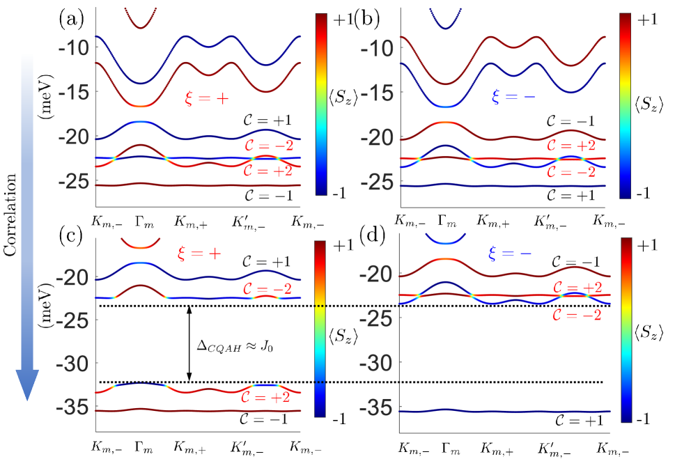
Figure S3: (a)-(b) Non-interacting bands of twisted homobilayer MoS2 for (a) valley $\xi=+$, and (b) valley $\xi=-$ with Rashba strength $\alpha_{so}=30$ meV$\cdot$ Å. Dashed lines in (a)-(b) indicate location of the Fermi energy EF when the 2${}^{\text{nd}}$ moiré bands are $1/2$-filled and interaction effects are neglected. In the absence of correlations, both bands from valley $\xi=+$ and valley $\xi=-$ are half-filled. (c)-(d) Correlated band structures when the 2${}^{\text{nd}}$ moiré bands are half-filled, where the system enters the valley-polarized state. Electron correlations induce an insulating gap $\Delta_{CQAH}\sim J_{0}$, where we set $J_{0}=10$ meVs.

IV. Estimate of spatial variation in Rashba SOC strength

As we discussed in the Conclusion and Discussion section in the main text, the formation of moiré pattern in principle leads to spatial variations of the Rashba SOC strength on the moiré scale (the amplitude of variations denoted by $\delta\alpha_{so}$ in the following).

To estimate $\delta\alpha_{so}$, the key observation is that the spatial variation in Rashba strength is not independent of the moiré potential. In particular, the moiré potential causes a spatial variation in the inter-layer potential differences between the two constituent layers with its amplitude on the scale of $V_{M}\approx 10$ meVs (Table I of the main text). Given the inter-layer distance $d=7{\AA}$ in bilayer MoS₂, this corresponds to a spatially modulating electric field with the amplitude of variations given by $\delta E_{z}=1.4mV\cdot{\AA}^{-1}$. Assuming a linear scaling relation $\delta\alpha_{so}=\lambda\delta E_{z}$, we obtain an estimated value of $\delta\alpha_{so}\approx 0.08meV\cdot{\AA}$ by using a proportionality constant $\lambda=0.0625e\cdot{\AA}^{2}$ for MoS₂ extrapolated from Fig.7 of Refs.YaoS . Thus, the amplitude of the spatial variation in Rashba SOC is negligibly small compared to previous reports on gate-induced Rashba SOC with $\alpha_{so}\sim 30meV\cdot{\AA}$ in each layer BenjaminS . This justifies the use of a uniform Rashba SOC in our continuum model as a good approximation.

References

(1) Yuan Cao, Valla Fatemi, Ahmet Demir, Shiang Fang, Spencer L. Tomarken, Jason Y. Luo, Javier D. Sanchez-Yamagishi, Kenji Watanabe, Takashi Taniguchi, Efthimios Kaxiras, Ray C. Ashoori & Pablo Jarillo-Herrero, Correlated insulator behaviour at half-filling in magic-angle graphene superlattices, Nature 556, 80-84 (2018).
(2) Yuan Cao, Valla Fatemi, Shiang Fang, Kenji Watanabe, Takashi Taniguchi, Efthimios Kaxiras & Pablo Jarillo-Herrero, Unconventional superconductivity in magic-angle graphene superlattices, Nature 556, 43–50 (2018).
(3) Stephen Carr, Daniel Massatt, Shiang Fang, Paul Cazeaux, Mitchell Luskin, and Efthimios Kaxiras, Twistronics: Manipulating the electronic properties of two-dimensional layered structures through their twist angle, Phys. Rev. B 95, 075420 (2017).
(6) Po, H. C., Zou, L., Vishwanath, A. & Senthil, T., Origin of Mott Insulating Behavior and Superconductivity in Twisted Bilayer Graphene, Phys. Rev. X 8, 031089 (2018).
(7) Noah F. Q. Yuan and Liang Fu, Model for the metal-insulator transition in graphene superlattices and beyond, Phys. Rev. B 98, 045103 (2018).
(8) Mikito Koshino et al., Maximally Localized Wannier Orbitals and the Extended Hubbard Model for Twisted Bilayer Graphene, Phys. Rev. X 8, 031087 (2018).
(9) Hiroki Isobe, Noah F. Q. Yuan and Liang Fu, Unconventional Superconductivity and Density Waves in Twisted Bilayer Graphene, Phys. Rev. X 8, 041041 (2018).
(10) Jian Kang and Oskar Vafek, Symmetry, Maximally Localized Wannier States, and a Low-Energy Model for Twisted Bilayer Graphene Narrow Bands, Phys. Rev. X 8, 031088 (2018).
(11) Fengcheng Wu, A. H. MacDonald, and Ivar Martin, Theory of Phonon-Mediated Superconductivity in Twisted Bilayer Graphene, Phys. Rev. Lett. 121, 257001 (2018).
(12) Cheng-Cheng Liu, Li-Da Zhang, Wei-Qiang Chen, and Fan Yang, Chiral Spin Density Wave and Superconductivity in the Magic-Angle-Twisted Bilayer Graphene, Phys. Rev. Lett. 121, 217001 (2018).
(13) Biao Lian, Zhijun Wang, and B. Andrei Bernevig, Twisted Bilayer Graphene: A Phonon-Driven Superconductor, Phys. Rev. Lett. 122, 257002 (2019).
(15) Ming Xie and A. H. MacDonald, Nature of the Correlated Insulator States in Twisted Bilayer Graphene, Phys. Rev. Lett. 124, 097601 (2020).
(16) Yuhang Jiang, Xinyuan Lai, Kenji Watanabe, Takashi Taniguchi, Kristjan Haule, Jinhai Mao & Eva Y. Andrei, Charge order and broken rotational symmetry in magic-angle twisted bilayer graphene, Nature 573, 91–95 (2019).
(17) Xiaobo Lu, Petr Stepanov, Wei Yang, Ming Xie, Mohammed Ali Aamir, Ipsita Das, Carles Urgell, Kenji Watanabe, Takashi Taniguchi, Guangyu Zhang, Adrian Bachtold, Allan H. MacDonald & Dmitri K. Efetov, Superconductors, orbital magnets and correlated states in magic-angle bilayer graphene, Nature 574, 653–657 (2019).
(18) Youngjoon Choi, Jeannette Kemmer, Yang Peng, Alex Thomson, Harpreet Arora, Robert Polski, Yiran Zhang, Hechen Ren, Jason Alicea, Gil Refael, Felix von Oppen, Kenji Watanabe, Takashi Taniguchi & Stevan Nadj-Perge, Electronic correlations in twisted bilayer graphene near the magic angle, Nature Physics 15, 1174–1180 (2019).
(19) Yonglong Xie, Biao Lian, Berthold Jäck, Xiaomeng Liu, Cheng-Li Chiu, Kenji Watanabe, Takashi Taniguchi, B. Andrei Bernevig & Ali Yazdani, Spectroscopic signatures of many-body correlations in magic-angle twisted bilayer graphene, Nature 572, 101–105 (2019).
(20) Jianpeng Liu, Junwei Liu, and Xi Dai, Pseudo Landau level representation of twisted bilayer graphene: Band topology and implications on the correlated insulating phase, Phys. Rev. B 99, 155415 (2019).
(21) Zhida Song, Zhijun Wang, Wujun Shi, Gang Li, Chen Fang, and B. Andrei Bernevig, All Magic Angles in Twisted Bilayer Graphene are Topological, Phys. Rev. Lett. 123, 036401 (2019).
(22) Nick Bultinck, Shubhayu Chatterjee, and Michael P. Zaletel, Mechanism for Anomalous Hall Ferromagnetism in Twisted Bilayer Graphene, Phys. Rev. Lett. 124, 166601 (2020).
(23) Ya-Hui Zhang, Dan Mao, Yuan Cao, Pablo Jarillo-Herrero, and T. Senthil, Nearly flat Chern bands in moiré superlattices, Phys. Rev. B 99, 075127 (2019).
(24) Ya-Hui Zhang, Dan Mao, and T. Senthil, Twisted bilayer graphene aligned with hexagonal boron nitride: Anomalous Hall effect and a lattice model, Phys. Rev. Research 1, 033126 (2019).
(25) Wen-Yu He, David Goldhaber-Gordon & K. T. Law, Giant orbital magnetoelectric effect and current-induced magnetization switching in twisted bilayer graphene, Nature Communications 11, 1650 (2020).
(26) Aaron L. Sharpe, Eli J. Fox, Arthur W. Barnard, Joe Finney, Kenji Watanabe, Takashi Taniguchi, M. A. Kastner, David Goldhaber-Gordon, Emergent ferromagnetism near three-quarters filling in twisted bilayer graphene, Science 365, 605-608 (2019).
(27) M. Serlin, C. L. Tschirhart, H. Polshyn, Y. Zhang, J. Zhu, K. Watanabe, T. Taniguchi, L. Balents, A. F. Young, Intrinsic quantized anomalous Hall effect in a moiré heterostructure, Science 367, 900-903 (2020).
(28) Kevin P. Nuckolls, Myungchul Oh, Dillon Wong, Biao Lian, Kenji Watanabe, Takashi Taniguchi, B. Andrei Bernevig & Ali Yazdani, Strongly correlated Chern insulators in magic-angle twisted bilayer graphene, Nature 588, 610–615 (2020).
(29) Fengcheng Wu, Timothy Lovorn, Emanuel Tutuc, Ivar Martin and A. H. MacDonald, Topological Insulators in Twisted Transition Metal Dichalcogenide Homobilayers, Phys. Rev. Lett. 122, 086402 (2019).
(30) Fengcheng Wu, Timothy Lovorn, Emanuel Tutuc, and A. H. MacDonald, Hubbard Model Physics in Transition Metal Dichalcogenide Moiré Bands, Phys. Rev. Lett. 121, 026402 (2018).
(31) Zhiming Zhang, Yimeng Wang, Kenji Watanabe, Takashi Taniguchi, Keiji Ueno, Emanuel Tutuc & Brian J. LeRoy, Flat bands in twisted bilayer transition metal dichalcogenides, Nature Physics 16, 1093–1096 (2020).
(32) Yanhao Tang, Lizhong Li, Tingxin Li, Yang Xu, Song Liu, Katayun Barmak, Kenji Watanabe, Takashi Taniguchi, Allan H. MacDonald, Jie Shan & Kin Fai Mak, Simulation of Hubbard model physics in WSe2/WS2 moiré superlattices, Nature 579, 353–358 (2020).
(33) Emma C. Regan et al., Mott and generalized Wigner crystal states in WSe2/WS2 moiré superlattices, Nature 579, 359–363 (2020).
(34) Lei Wang et al., Correlated electronic phases in twisted bilayer transition metal dichalcogenides, Nature Materials 19, 861–866 (2020).
(35) Zhen Bi and Liang Fu, Excitonic density wave and spin-valley superfluid in bilayer transition metal dichalcogenide, Nature Communications 12, 642 (2021).
(36) Oguzhan Can, Tarun Tummuru, Ryan P. Day, Ilya Elfimov, Andrea Damascelli & Marcel Franz, High-temperature topological superconductivity in twisted double-layer copper oxides,Nature Physics 17, 519–524 (2021).
(37) Pavel A. Volkov, Justin H. Wilson, J. H. Pixley, Magic angles and current-induced topology in twisted nodal superconductors, arXiv:2012.07860
(38) Di Xiao, Gui-Bin Liu, Wanxiang Feng, Xiaodong Xu, and Wang Yao, Coupled Spin and Valley Physics in Monolayers of MoS2 and Other Group-VI Dichalcogenides, Phys. Rev. Lett. 108, 196802 (2012).
(39) Gui-Bin Liu, Wen-Yu Shan, Yugui Yao, Wang Yao, and Di Xiao, Three-band tight-binding model for monolayers of group-VIB transition metal dichalcogenides, Phys. Rev. B 88, 085433 (2013).
(40) K. Kośmider, J. W. González, and J. Fernández-Rossier, Large spin splitting in the conduction band of transition metal dichalcogenide monolayers, Phys. Rev. B 88, 245436 (2013).
(41) Benjamin T. Zhou, Katsuhisa Taguchi, Yuki Kawaguchi, Yukio Tanaka & K. T. Law, Spin-orbit coupling induced valley Hall effects in transition-metal dichalcogenides, Communications Physics 2, 26 (2019).
(42) K. Taguchi, B. T. Zhou, Y. Kawaguchi, Y. Tanaka, and K. T. Law, Valley Edelstein effect in monolayer transition-metal dichalcogenides, Phys. Rev. B 98, 035435 (2018).
(43) Kyung-Han Kim and Hyun-Woo Lee, Berry curvature in monolayer MoS2 with broken mirror symmetry, Phys. Rev. B 97, 235423 (2018).
(44) See the Supplemental Material for details on: (i) calculation of effective inter-layer tunneling parameter ; (ii) method used for computing Chern numbers in the moiré bands; (iii) self-consistent Hartree-Fock calculations for correlated ground at 1/2-filling and discussions on the case of general filling; (iv) estimate of spatial variation in Rashba SOC strength, which includes Refs.Sun ; Zahid ; Suzuki ; Yao .
(46) Kin Fai Mak, Changgu Lee, James Hone, Jie Shan, and Tony F. Heinz, Atomically Thin
MoS2: A New Direct-Gap Semiconductor, Phys. Rev. Lett. 105, 136805 (2010).
(48) Ferdows Zahid, Lei Liu, Yu Zhu, Jian Wang, and Hong Guo, A generic tight-binding model for monolayer, bilayer and bulk MoS2, AIP Advances 3, 052111 (2013).
(49) Takahiro Fukui, Yasuhiro Hatsugai, and Hiroshi Suzuki, Chern Numbers in Discretized Brillouin Zone: Efficient Method of Computing (Spin) Hall Conductances, J. Phys. Soc. Jpn. 74, 1674
(2005).
(50) Qun-Fang Yao, Jia Cai, Wen-Yi Tong, Shi-Jing Gong, Ji-Qing Wang, Xiangang Wan, Chun-Gang Duan, and J. H. Chu, Manipulation of the large Rashba spin splitting in polar two-dimensional transition-metal dichalcogenides, Phys. Rev. B 95, 165401 (2017).
Supplemental Material for
“Moiré Chern bands and correlated quantum anomalous Hall states