The HCCL Speaker Verification System for Far-Field Speaker Verification Challenge

Abstract

This paper describes the systems submitted by team HCCL to the Far-Field Speaker Verification Challenge. Our previous work in the AIshell Speaker Verification Challenge 2019 shows that the powerful modeling abilities of Neural Network architectures can provide exceptional performence for this kind of task. Therefore, in this challenge, we focus on constructing deep Neural Network architectures based on TDNN, Resnet and Res2net blocks. Most of the developed systems consist of Neural Network embeddings are applied with PLDA backend. Firstly, the speed perturbation method is applied to augment data and significant performance improvements are achieved. Then, we explore the use of AMsoftmax loss function and propose to join a CE-loss branch when we train model using AMsoftmax loss. In addition, the impact of score normalization on perfomance is also investigated. The final system, a fusion of four systems, achieves minDCF 0.5342, EER 5.05% on task1 eval set, and achieves minDCF 0.5193, EER 5.47% on task3 eval set.

Index Terms: speaker verification, speed perturbation, text-dependent, ftdnn, Resnet, Res2net, AMsoftmax loss

1 Introduction

In the past decade, with the development of deep learning, speaker verification technology has significantly advanced in telephone channel and close-talking. Recently, due to its extensive applications in smart home and smart city, speaker verification under far-filed and complex environment has aroused great interest in research and authentic applications. However, with the adverse impacts of the long-range fading, room reverberation, and complex environmental noises, etc., far-field speaker verification is still challenging.

In this paper, we describe the speaker verification systems developed by the team HCCL for the FFSVC2020 challenge[1]. The challenge aims to benchmark the state-of-the-art speaker verification technology under far-field and noisy conditions, meanwhile, promote the development of new ideas and techniques in speaker verification. The challenge has three tasks, far-field text-dependent speaker verification from single microphone array, far-field text-independent speaker verification from single microphone array and far-field text-dependent speaker verification from distributed microphone array. Our team mainly participate in task1 and task3.

According to our prior work in the AIshell Speaker Verification Challenge 2019[2], we explore several deep speaker embedding extractors based on TDNN(Time Delay Neural Network)[3], Resnet(Residual Neural Network)[4] blocks and Res2net[5] blocks in this challenge. In addition, the impact of data augmentation, loss function, backend strategies and score normalization techniques on systems performance is also analyzed.

2 System description

This section describes the systems we develope for the FFSVC2020 challenge. Firstly, we introduce the datasets, data augmentation and spectral feature used in model training. Secondly, we introduce several state-of-the-art models, including the common TDNN xvector architecture[6], ETDNN(Extended TDNN) xvector architecture[7][8], FTDNN(Factorized TDNN) xvector architecture[9], Resnet[4][10][11][12] architecture and Res2net[4] architecture. Specially, we explore a unique resnet model, Res2net50 model, which proposed in paper[5]. Thirdly, we explore the use of AMsoftmax(the Additive Margin Softmax)[13] loss to improve the performance. Finally, some backend methods, such as PLDA(Probabilistic Linear Discriminant Analysis)[14][15], EDA(Enrollment Data Augmentation)[2], ASnorm(Adaptive Symmetric Score Normalization)[16] and scores fusions are described.

2.1 Training data preparation

The training sets used in our experiments are VoxCeleb-1+2[17][18], AIshell[19][20], HIMIA[2] and part of the DMASH Dataset that FFSVC2020[21] provides.

The challenge provides a training set with 120 speakers, and a development set with 35 speakers. The HIMIA dataset has 254 speakers in the training set and 42 speakers in the developement set. There are 405 speakers in total after excluding duplicates in two data sets. For each text-dependent utterance in the HIMIA dataset, we use the recordings from four recording devices, which include one 25cm distance microphone and three randomly selected microphone arrays (4 channels per array). For the sake of clarity, the datasets notations are defined as in table 1.

In order to increase the number of speakers in the HIMIA dataset and FFSVC dataset, the speed perturbation[22][23] method is introduced to creat copies of the original signal with speed factors of 0.8, 0.9 and 1.1 using standard Kaldi[24] speed perturbation recipe. Because the speed perturbation results in changed speech spectrum, the copies are considered to belong to another speaker which differs from the original. In this way, the number of speakers grows a lot.

For the purpose of increasing the amount and the diversity of the training data, all training data, including copies created by the speed perturbation, is augmented by using the freely available MUSAN[25] and RIRs datasets, creating four corrupted copies of the original recordings with Kaldi recipe.

Table 1: Datasets Notations

notation	datasets	augmentation	num spks
Vox	Voxceleb 1+2	noise aug	7363
Vox1	Voxceleb 1	noise aug	1211
AIshell	AIshell	noise aug	2401
FFSVC405	FFSVCdata + HiMIA	noise aug	405
FFSVC1215	FFSVCdata + HiMIA	noise + speed 0.9, 1.1 aug	405*3
FFSVC1620	FFSVCdata + HiMIA	noise + speed 0.8, 0.9, 1.1 aug	405*4

2.2 Feature extraction

All training datasets are resampled to 16kHz and pre-emphasized before feature extraction. 30-dimensional MFCCs (Mel Frequency Cepstral Coefficients) extracted from 25ms frames with 10 ms overlop, spanning the frequency range 20Hz-7600Hz and 64-dimensional MFB (Log Mel-filter Bank Energies) from 25ms frames with 10ms overlop, with frequency limits 0-8000Hz are used in this challenge.

2.3 Embedding Extractors

The systems based on TDNN used by our team include xvector, ETDNN xvector, FTDNN xvector. The systems based on Resnet blocks use in this challenge name Resnet34 and Resnet50.

Res2net block is a modified version of Resnet block, as shown in Figure 1. The 3*3 filters are replaced by several smaller filter groups, and these outputs are concatenated after convolution operations. There are two important parameters, width and scale. Scale represents the number of groups that one $3*3$ filter is split into. Width represents the number of channels of each small group. For details, please refer to the paper A unique multi-scale architecture for text-independent speaker verification, which is submitted by our laboratory to interspeech2020.

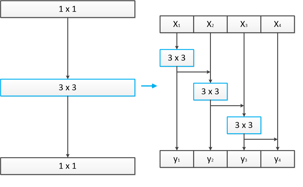
Figure 1: Simplified Res2Net Block

2.4 Loss Function

Recent studies have shown that AMsoftmax loss has greatly improved performance in the field of speaker verification[26]. We also use AMsoftmax in this challenge. Meanwhile, we add CE-loss branch to the network to do joint training. The AMsoftmax loss function is formulated as:

$$L_{AMS}=\frac{1}{N}\sum_{i}-log\frac{e^{s*(cos\theta_{y_{i}}-m)}}{e^{s*(cos\theta_{y_{i}}-m)}+\sum_{j\not=y_{i}}e^{s*cos(\theta_{y_{j}},i)}}$$

where $s$ is a scale factor and $m$ is the margin factor.

2.5 Backend

In this work, either CS(cosine similarity) or PLDA is used for scoring. Additionally, EDA and ASnorm are also applied.

2.5.1 Enrollment Data Augmentation

There is a large mismatch between the enrollmenat and the test utterances because of the different recording environments. Recent researches have shown that it’s an effective method to relif this mismatch by using MUSAN and RIRs dataset to augment enrollment utterances[2][21]. The final enrollment embedding is obtained by averaging the embedding from the original uttrance and the augmented versions.

2.5.2 Score Normalization

Finally, ASnorm scheme is also adopted as proposed in [16]. For every pair $(x_{1},x_{2})$, the normalized score can be calculated as follows:

$$\hat{S}(x_{1},x_{2})=\frac{S(x_{1},x_{2})-\mu_{1}}{\sigma_{1}}+\frac{S(x_{1},x_{2})-\mu_{2}}{\sigma_{2}}$$

Here, $\mu_{1}$ and $\sigma_{1}$ are calculated by matching $x_{1}$ against the cohort set and similarly for $\mu_{2}$ and $\sigma_{2}$. Means and standard deviations are calculated using a set of $N$ best scoring impostors.

3 Implementation, Result and Analyze

We develop three series of systems based on TDNN and Resnet blocks, including Resnet systems used pyTorch, TDNN systems used Kaldi[24], TDNN systems used pyTorch. The first series are built using pyTorch, and based on Resnet and Res2net model. The second series are built using the Kaldi toolkit, and the TDNN and ETDNN xvector models are first pre-trained, then FFSVC2020 train-dataset and HIMIA dataset are used to finetune the model. The third series are built using pyTorch, and the ETDNN and FTDNN xvector models are trained only using FFSVC2020 train-dataset and HIMIA dataset. In addition, we explain the naming rules which is followed throughout this paper for all systems. The naming rules are divided into two categories, finetune and non-finetune. The first is named as $\langle$the training data used for base model$\rangle$-$\langle$feature$\rangle$-$\langle$architecture$\rangle$-$\langle$the training data used for finetune$\rangle$-$\langle$feature$\rangle$-finetune, and the second is named as $\langle$the training data used for model$\rangle$-$\langle$feature$\rangle$-$\langle$architecture$\rangle$(-$\langle$loss function$\rangle$).

3.1 Resnet systems used pyTorch

All systems in this series are implemented with pyTorch and use MFB as input feature. Meanwhile, dropout is applied to embedding layer, and CS is used for scores in this series. In addition, EDA is used in all results, including other series.

Vox1-MFB-Resnet34-FFSVC405-MFB-finetune: Considering the number of speakers in FFSVC405, finetune is a good transfer learning method for this challenge. The Resnet34 model, which described in [10], is pre-trained with 1211 speakers in Vox1-MFB. The widths (number of channels) of the residual blocks used in our experiments are {32,64,128,256}. In this stage, the model is trained using stochastic gradient descent with weight decay 1e-4 and momentum 0.9. The learning rate is set to 0.1, 0.01, 0.001 and is switched when the training loss plateaus. After the pre-trained model converges, FFSVC405-MFB is used to finetune the model with the learning rate 0.001.

FFSVC405-MFB-Resnet34: For comparison, the resnet34 model is directly trained with FFSVC405-MFB. Stochastic gradient descent optimization is used with weight decay 1e-4 and momentum 0.9. The learning rate is set to 0.1, 0.01, 0.001 and is switched when the training loss plateaus.

In order to facilitate the training of PLDA, the embedding-size is expanded from the original 128 dimensions to 512 dimensions. The impact of embedding size on performance is also explored by comparative experiments. Meanwhile, Spectrum masking[27] is used in our training stage, and masking 5%-10% of the Spectrogram for each utterance. The results are summarized in Table 2, and all scores in this Table use CS for scoring. It could find that embedding size has no effect on system performance, spectrum masking can yield a 3%-5% relative improvement in EER and minDCF, finetune can yield about 8% relative improvement in EER and 2%-4% improvement in minDCF.

Table 2: Research of mask and embedding size

system	embedding size	mask	minDCF	EER
Vox1-MFB	128	no	0.721	6.49
-Resnet34-	128	yes	0.690	6.22
FFSVC405	512	no	0.719	6.49
-MFB-fintune	512	yes	0.677	6.28
	128	no	0.738	7.16
FFSVC405	128	yes	0.705	6.75
-MFB-Resnet34	512	no	0.729	6.98
	512	yes	0.722	6.78

Vox1-MFB-Resnet34-FFSVC1215-MFB-finetune: This extractor is similar to Vox1-MFB-Resnet34-FFSVC405-MFB-finetune, with the difference of using FFSVC1215-MFB to finetune.

AIshell-MFB-Resnet34-FFSVC1215-MFB-finetune: This extractor is similar to Vox1-MFB-Resnet34-FFSVC1215-MFB-finetune, with the difference of using AIshell-MFB, 2401 spks, to pre-train the model.

FFSVC1215-MFB-Resnet34: This extractor is similar to FFSVC405-MFB-Resnet34, with the difference of using FFSVC1215-MFB to finetune.

FFSVC1215-MFB-Res2net50: This extractor is similar to FFSVC1215-MFB-Resnet34, with the difference of using Res2net50 embedding extractor, with width 16 and scale 4.

FFSVC1620-MFB-Resnet34: This extractor is similar to FFSVC405-MFB-Resnet34, with the difference of using FFSVC1215-MFB to finetune.

FFSVC1620-MFB-Res2net50: This extractor is similar to FFSVC1215-MFB-Resnet34, with the difference of using Res2net50 embedding extractor.

The results of this six systems are summarized in Table 3. It could find that the dataset used for pre-training has little effect on the final performance, and finetune is no longer effective when the number of speakers in datasets is comparable to the pre-training set. It is interesting that speed perturbation with speed factors of 0.9 and 1.1 achieves about 10% relative improvement in EER and 6% improvement in minDCF. Therefore, we draw the conclusion that speed perturbation is an effective data augmentation method to prevent over-fitting when numbers of speakers is not enough. In addition, Res2net blocks improves the performance by 3% relatively compared to Resnet blocks. Res2net blocks could get more receptive field to improve the multi-scale feature extraction ability by using scale and width so that Res2net blocks obtains better performance than Resnet blocks.

Table 3: Results of series of Resnet systems

system	minDCF	EER
Vox1-MFB-Resnet34-
FFSVC1215-MFB-finetune	0.689	6.13
AIshell-MFB-Resnet34-
FFSVC1215-MFB-finetune	0.695	6.02
FFSVC1215-MFB-Resnet34	0.648	5.62
FFSVC1215-MFB-Res2net50	0.630	5.49
FFSVC1620-MFB-Resnet34	0.639	5.37
FFSVC1620-MFB-Res2net50	0.620	5.30

3.2 TDNN systems used Kaldi

All systems in this series are implemented with Kaldi and MFCC are used as input feature. In addition, all embeddings are transformed to 200 dimension using LDA, and then unit-length normalization and standard PLDA are applied. LDA/PLDA is trained on the finetune dataset. Here, xvector represents the common TDNN xvector model.

AIshell-MFCC-xvector-FFSVC1620-MFCC-finetune: According to the Resnet series systems, AIshell-MFCC is used to pretrain xvector model, then FFSVC1620-MFCC is used to finetune. The model is finetuned with an initial learning rate of 0.001 and a final learning rate of 0.0001.

AIshell-MFCC-xvector-FFSVC405-MFCC-finetune: This extractor is similar to AIshell-MFCC-xvector-FFSVC1620 -MFCC-finetune, with the difference of using FFSVC405-MFCC to finetune.

AIshell-MFCC-ETDNN-FFSVC1620-MFCC-finetune: This extractor is similar to AIshell-MFCC-xvector-FFSVC1620 -MFCC-finetune. However, the model to pre-train is ETDNN xvector.

Table 4: Research of backend technique

System	cosine		PLDA scoring		Asnorm
	minDCF	EER	minDCF	EER	minDCF	EER
FFSVC1620-MFB-Resnet34	0.639	5.37	0.630	5.33	0.561	5.24
FFSVC1620-MFB-Res2net50	0.620	5.30	0.621	5.22	0.547	5.16
AIshell-MFCC-xvector-FFSVC1215-MFCC-finetune	-	-	0.576	5.20	0.514	4.67
FFSVC1215-MFB-FTDNN-CEAMS	0.555	5.19	0.534	4.72	0.508	4.61

AIshell-MFCC-xvector-FFSVC1215-MFCC-finetune: This extractor is similar to AIshell-MFCC-xvector-FFSVC1620 -MFCC-finetune, with the difference of the finetune dataset. Only part of FFSVC1215-MFCC is used to finetune the base model. During the finetune stage, the accuracy of the training dataset increases rapidly to 99%, and the valid dataset is also rapidly maintained at 96%. So, we attempt to increase difficulty by remove the clean data from close-talking mic in the HIMIA dataset. Meanwhile, considering to channel mismatch between the close-talking enrollment utterance from cellphone and the far-field testing speech from microphone, the recordings from 25cm distance cellphone in The DMASH dataset is not removed. In addition, the impact of the learning rate during finetune stage is explored in our experiments. we attempt to fix the first 6 layers with the learning rate of 0.001-0.0001, and then we untie the fixed layer with the learning rate of 0.0001-0.00005, we named this system AIshell-MFCC-xvector-FFSVC1215-MFCC-finetune-V02. The results of these five systems are shown in Table 5.

Table 5: Results of series of TDNN-Kaldi systems

system	minDCF	EER
AIshell-MFCC-xvector-
FFSVC405-MFCC-finetune	0.768	7.36
AIshell-MFCC-xvector-
FFSVC1620-MFCC-finetune	0.612	5.82
AIshell-MFCC-ETDNN-
FFSVC1620-MFCC-finetune	0.671	6.21
AIshell-MFCC-xvector-
FFSVC1215-MFCC-finetune	0.576	5.20
AIshell-MFCC-xvector-
FFSVC1215-MFCC-finetune-V02	0.599	5.52

3.3 TDNN systems used pyTorch

All systems in this series are implemented with pyTorch and use MFB as input feature. Particularly, AMS represents the AMsoftmax loss is adopted in model training, CEAMS represents that the CE-loss branch is added when we train the models using AMsoftmax loss.

FFSVC1215-MFB-ETDNN-AMS: This extractor is similar to FFSVC1215-MFB-Resnet34, with the difference of using ETDNN model and AMsoftmax loss function. Parameters $m$ and $s$ are respectively equal to 0.1 and 30 during the whole training stage. In addition, weight decay uses 1e-3.

FFSVC1215-MFB-FTDNN-AMS: This extractor is similar to FFSVC1215-MFB-ETDNN-AMS, with the difference of using FTDNN model.

FFSVC1215-MFB-FTDNN-CEAMS: This extractor is similar to FFSVC1215-MFB-ETDNN-AMS, with the difference of using CEAMsoftmax loss. During the training stage using AMsoftmax loss, the training process is extremely unstable, and is very prone to overfit, especially when parameters $m$ is greater than 0.1. Although the copies which are created by using speed perturbation is considered to belong to diffrent speakers, it’s similar to the original signal to some extent. In addition, the deep network is prone to overfit when small-scale training data is available, not to mention similar uttrances. To address this problems, CE-loss is added to the network to guide and assist the model training in the early stage. We first add a CE-loss class prediction branch to conventional feedforward architecture in parallel with the AMsoftmax-loss class prediction branch, in practice, the CE-loss class prediction branch is added after the statistics pooling layer of the FTDNN network, and has the same network structure as the AMsoftmax-loss branch. The weight of CE-loss is set to 1.0, 0.5, 0.1 and is switched when the training loss plateaus.

FFSVC1620-MFB-FTDNN-CEAMS: This extractor is similar to FFSVC1215-MFB-ETDNN-AMS, with the difference of using FFSVC1620-MFB.

Table 6: Results of series of TDNN-pyTorch systems

system	minDCF	EER
FFSVC1215-MFB-ETDNN-AMS	0.698	6.57
FFSVC1215-MFB-FTDNN-AMS	0.609	6.27
FFSVC1215-MFB-FTDNN-CEAMS	0.555	5.21
FFSVC1620-MFB-FTDNN-CEAMS	0.534	5.18

The results of the above four models are summarized in Table 6. During the experiment, the model training stability has been greatly improved after adding CE-loss branch, and it achieves about 8% relative improvement in minDCF and 16% improvement in EER.

3.4 Backend

We select four of the best models to do backend scoring. The methods we use includes LDA, PLDA, ASnorm and score fusion. All of the four models use PLDA scoring and ASnorm. Firstly, for systems implemented with pytorch, we transform the centered, whitened, and unit-length normalized embeddings by LDA, without dimensionality reduction. Then, one Gaussian PLDA is trained either on FFSVC1215 or FFSVC1620 set. Finally, we use ASnorm to post-process the PLDA verification. We use the eval set and dev set as each other’s cohort set. For each enrollment from 25cm distance cellphone, we randomly select 2700 single far-field microphone arrays from the cohort set to score with it, each testing utterance is similar. Then we select the top 5% of sorted cohort scores to calculate the normalization. The result of these four systems are shown in Table 4.

3.5 Submitted system and result

We submit the fusion results of the above four systems. Considering that task1 and task3 are similar, we use the same models in these two tasks. These four systems are renamed as follows, FFSVC1620-MFB-Resnet34 named system A,FFSVC1620-MFB-Res2net50 named system B, AIshell-MFCC-xvector-FFSVC1215-MFCC-finetune named system C, FFSVC1215-MFB-FTDNN-CEAMS named system D. The fusion results are summarized in Table 7.

Table 7: results of submitted systems

System	task1 dev		task1 eval		task3 eval
	minDCF	EER	minDCF	EER	minDCF	EER
A+C+D	0.442	3.88	0.549	5.08	0.526	5.61
A+B+C+D	0.427	3.70	0.534	5.05	0.519	5.47

4 Conclusions

In this paper, we detail every aspects of our systems submitted to FFSVC2020 challenge. We describe the usage of data sets, the strategy of data augmentation, various embedding extractors, backend technique. Our data augmentation strategy is greatly helpful when only small-scale training data is available. In addition, AMsoftmax loss will be easier to ultilize after adding CE-loss branch. Res2net block could improve performance by getting multi-scale feature infomation. The above three points might be useful to other researchers. Finally, we don’t make full use of the infomation between multi-channel, we will explore how to ultilize these infomations in the future.

5 Acknowledgements

This work is partially supported by the National Natural Science Foundation of China (Nos. 11590772,11590770).

References

- [1] X. Qin, M. Li, H. Bu, R. K. Das, W. Rao, S. Narayanan, and H. Li, “The ffsvc 2020 evaluation plan,” arXiv preprint arXiv:2002.00387, 2020.
- [2] X. Qin, H. Bu, and M. Li, “Hi-mia: A far-field text-dependent speaker verification database and the baselines,” in 2020 IEEE International Conference on Acoustics, Speech and Signal Processing (ICASSP). IEEE, 2020, pp. 7609–7614.
- [3] D. Snyder, D. Garcia-Romero, and D. Povey, “Time delay deep neural network-based universal background models for speaker recognition,” in 2015 IEEE Workshop on Automatic Speech Recognition and Understanding (ASRU). IEEE, 2015, pp. 92–97.
- [4] K. He, X. Zhang, S. Ren, and J. Sun, “Deep residual learning for image recognition,” in Proceedings of the IEEE conference on computer vision and pattern recognition, 2016, pp. 770–778.
- [5] S. Gao, M.-M. Cheng, K. Zhao, X.-Y. Zhang, M.-H. Yang, and P. H. Torr, “Res2net: A new multi-scale backbone architecture,” IEEE transactions on pattern analysis and machine intelligence, 2019.
- [6] D. Snyder, D. Garcia-Romero, D. Povey, and S. Khudanpur, “Deep neural network embeddings for text-independent speaker verification.” in Interspeech, 2017, pp. 999–1003.
- [7] D. Snyder, D. Garcia-Romero, G. Sell, D. Povey, and S. Khudanpur, “X-vectors: Robust dnn embeddings for speaker recognition,” in 2018 IEEE International Conference on Acoustics, Speech and Signal Processing (ICASSP). IEEE, 2018, pp. 5329–5333.
- [8] D. Snyder, D. Garcia-Romero, G. Sell, A. McCree, D. Povey, and S. Khudanpur, “Speaker recognition for multi-speaker conversations using x-vectors,” in ICASSP 2019-2019 IEEE International Conference on Acoustics, Speech and Signal Processing (ICASSP). IEEE, 2019, pp. 5796–5800.
- [9] D. Povey, G. Cheng, Y. Wang, K. Li, H. Xu, M. Yarmohammadi, and S. Khudanpur, “Semi-orthogonal low-rank matrix factorization for deep neural networks.” in Interspeech, 2018, pp. 3743–3747.
- [10] W. Cai, J. Chen, and M. Li, “Exploring the encoding layer and loss function in end-to-end speaker and language recognition system.” in Proc. of Odyssey, 2018, pp. 74–81.
- [11] J. Villalba, N. Chen, D. Snyder, D. Garcia-Romero, A. McCree, G. Sell, J. Borgstrom, L. P. García-Perera, F. Richardson, R. Dehak et al., “State-of-the-art speaker recognition with neural network embeddings in nist sre18 and speakers in the wild evaluations,” Computer Speech & Language, vol. 60, p. 101026, 2020.
- [12] A. Gusev, V. Volokhov, T. Andzhukaev, S. Novoselov, G. Lavrentyeva, M. Volkova, A. Gazizullina, A. Shulipa, A. Gorlanov, A. Avdeeva et al., “Deep speaker embeddings for far-field speaker recognition on short utterances,” arXiv preprint arXiv:2002.06033, 2020.
- [13] F. Wang, J. Cheng, W. Liu, and H. Liu, “Additive margin softmax for face verification,” IEEE Signal Processing Letters, vol. 25, no. 7, pp. 926–930, 2018.
- [14] S. Ioffe, “Probabilistic linear discriminant analysis,” in European Conference on Computer Vision. Springer, 2006, pp. 531–542.
- [15] S. J. Prince and J. H. Elder, “Probabilistic linear discriminant analysis for inferences about identity,” in 2007 IEEE 11th International Conference on Computer Vision. IEEE, 2007, pp. 1–8.
- [16] S. Cumani, P. D. Batzu, D. Colibro, C. Vair, P. Laface, and V. Vasilakakis, “Comparison of speaker recognition approaches for real applications,” in Twelfth Annual Conference of the International Speech Communication Association, 2011.
- [17] A. Nagrani, J. S. Chung, and A. Zisserman, “Voxceleb: a large-scale speaker identification dataset,” arXiv preprint arXiv:1706.08612, 2017.
- [18] J. S. Chung, A. Nagrani, and A. Zisserman, “Voxceleb2: Deep speaker recognition,” arXiv preprint arXiv:1806.05622, 2018.
- [19] H. Bu, J. Du, X. Na, B. Wu, and H. Zheng, “Aishell-1: An open-source mandarin speech corpus and a speech recognition baseline,” in 2017 20th Conference of the Oriental Chapter of the International Coordinating Committee on Speech Databases and Speech I/O Systems and Assessment (O-COCOSDA). IEEE, 2017, pp. 1–5.
- [20] J. Du, X. Na, X. Liu, and H. Bu, “Aishell-2: transforming mandarin asr research into industrial scale,” arXiv preprint arXiv:1808.10583, 2018.
- [21] X. Qin, M. Li, H. Bu, W. Rao, R. K. Das, S. Narayanan, and H. Li, “The interspeech 2020 far-field speaker verification challenge,” in Interspeech 2020, 2020.
- [22] T. Ko, V. Peddinti, D. Povey, and S. Khudanpur, “Audio augmentation for speech recognition,” in Sixteenth Annual Conference of the International Speech Communication Association, 2015.
- [23] H. Yamamoto, K. A. Lee, K. Okabe, and T. Koshinaka, “Speaker augmentation and bandwidth extension for deep speaker embedding,” in Interspeech 2019, 2019, pp. 406–410.
- [24] D. Povey, A. Ghoshal, G. Boulianne, L. Burget, O. Glembek, N. Goel, M. Hannemann, P. Motlicek, Y. Qian, P. Schwarz et al., “The kaldi speech recognition toolkit,” in IEEE 2011 workshop on automatic speech recognition and understanding, no. CONF. IEEE Signal Processing Society, 2011.
- [25] D. Snyder, G. Chen, and D. Povey, “Musan: A music, speech, and noise corpus,” arXiv preprint arXiv:1510.08484, 2015.
- [26] Y. Liu, L. He, and J. Liu, “Large margin softmax loss for speaker verification,” in Interspeech 2019, 2019, pp. 2873–2877.
- [27] D. S. Park, W. Chan, Y. Zhang, C.-C. Chiu, B. Zoph, E. D. Cubuk, and Q. V. Le, “Specaugment: A simple data augmentation method for automatic speech recognition,” in Interspeech 2019, 2019, pp. 2613–2617.