On the Use of Field RR Lyrae as Galactic Probes. V. Optical and radial velocity curve templates

Abstract

We collected the largest spectroscopic catalog of RR Lyrae (RRLs) including $\approx$20,000 high-, medium- and low-resolution spectra for $\approx$10,000 RRLs. We provide the analytical forms of radial velocity curve (RVC) templates. These were built using 36 RRLs (31 fundamental—split into three period bins—and 5 first overtone pulsators) with well-sampled RVCs based on three groups of metallic lines (Fe, Mg, Na) and four Balmer lines (H_α, H_β, H_γ, H_δ). We tackled the long-standing problem of the reference epoch to anchor light curve and RVC templates. For the $V$-band, we found that the residuals of the templates anchored to the phase of the mean magnitude along the rising branch are $\sim$35% to $\sim$45% smaller than those anchored to the phase of maximum light. For the RVC, we used two independent reference epochs for metallic and Balmer lines and we verified that the residuals of the RVC templates anchored to the phase of mean RV are from 30% (metallic lines) up to 45% (Balmer lines) smaller than those anchored to the phase of minimum RV. We validated our RVC templates by using both the single- and the three-phase points approach. We found that barycentric velocities based on our RVC templates are two-three times more accurate than those available in the literature. We applied the current RVC templates to Balmer lines RVs of RRLs in the globular NGC 3201 collected with MUSE at VLT. We found the cluster barycentric RV of $V_{\gamma}$=496.89$\pm$8.37(error)$\pm$3.43 (standard deviation) km/s, which agrees well with literature estimates.

1 Introduction

Pulsating variables are behind numerous breakthroughs in astrophysics. Classical Cepheids (CCs) were used to estimate the distance to M31 and solve the Great Debate concerning the extragalactic nature of the so-called Nebulae (Hubble 1926) and to trace, for the first time, the rotation of the Galactic thin disc (Oort 1927; Joy 1939). The size and the age of the Universe were revolutionized thanks to the discovery of the difference between CCs, RRLs, and type II Cepheids (TIICs, Baade 1956). Indeed, while they were previously thought to represent the same type of variable stars, it became clear that they represented very distinct populations, with the RRLs and TIICs being very old (t$\geq$10 Gyr), and the CCs very young (t$\leq$300 Myr).

Nowadays, CCs are among the most popular calibrators of the extragalactic distance scale (Riess et al. 2019). RRLs, albeit fainter, are excellent standard candles that can provide robust, independent distance measurements even for stellar populations where the young CCs are absent. RRLs obey the well-defined Period-Luminosity-Metallicity (PLZ) relations for wavelengths longer than the $R$-band (Bono et al. 2003; Catelan 2009). As tracers of purely old stellar populations, they can be used to investigate the early formation and evolution of both the Galactic Halo (Fiorentino et al. 2015; Belokurov et al. 2018; Fabrizio et al. 2019) and Bulge (Pietrukowicz et al. 2015; Braga et al. 2018).

It is noteworthy that we lack general consensus on the Galactic Halo structure, in part because different stellar tracers provide different views concerning its spatial structure and the timescale for its formation. Indeed, Carollo et al. (2007) by using Main Sequence, subgiants and RGs and Kinman et al. (2012) by using RRLs, suggested that the outer halo is more spherical and its density profile is shallower when compared with the inner halo. In contrast, Keller et al. (2008) by using RRLs and Sesar et al. (2010, 2011) by using RRLs plus Main Sequence stars suggested that the outer halo has a steeper density profile when compared with the inner halo. Deason et al. (2011) by using Blue Horizontal Branch stars and Blue Stragglers found no change in the flattening as a function of the Galactocentric distance (Sesar et al. 2011). More recently, Xue et al. (2015), by adopting a global ellipsoidal stellar density model with Einasto profile found that the models with constant flattening provide a good fit to the entire Halo.

The tension between different measurements may be due to the sample selection of each study. On the one hand, the ages of the RRLs cover a narrow range from $\sim$10 to $\sim$13 Gyrs. There is evidence that a few RRLs—or stars that mimic RRLs, see Smolec et al. (2013)—are the aftermath of binary evolution, but they only represent a few percent of the populations (Bono et al. 1997; Pietrzyński et al. 2012; Kervella et al. 2019). On the other hand, Red giants (RGs) and main sequence (MS) stars, typically used to investigate the Halo, have only very weak age constraints (Conroy et al. 2021). Indeed, all stellar structures less massive than 2M_⊙ (older than $\sim$0.5-1.0 Gyr) experience a RG phase and MS stars also cover a broad range in stellar masses/ages. This means that if the Halo is the result of an in- tense disruption and merging activity (Monachesi et al. 2019) RG and MS stars are far from being optimal tracers of the early formation, because they are a mixed bag concerning the age dis- tribution.

Field RRLs are less numerous when compared with RG and MS stars, but their narrow age distribution makes them uniquely suited for Galactic archaeology. They probe a significant Halo fraction (Galactocentric distance $\leq$150 kpc) with high accuracy. Their individual distances have uncertainties on average smaller than 3-5% and their accuracy improves when moving from optical to NIR (Longmore et al. 1986; Catelan et al. 2004; Braga et al. 2015). This is a key advantage even in the Gaia era: Gaia EDR3 has an accuracy of 3% for Halo RRLs (G$\leq$15 mag) at 1 kpc and this accuracy will be extended to 2 kpc at the end of the mission (Clementini et al. 2019). RRLs are also valuable targets from the kinematical point of view. In fact, by measuring their velocities, one gets information on the kinematical state of the old population (Halo, Globular Clusters, Bulge). The pioneering work by Layden (1994, 1995), based on 302 RRLs, pointed towards a non-steady formation of the Halo, favouring a fragmented accretion scenario (Searle & Zinn 1978). More recently, Zinn et al. (2020) were able to pinpoint the membership of several Halo RRLs to past merger events (Gaia-Enceladus and the Helmi streams, Helmi et al. 1999; Myeong et al. 2018; Helmi et al. 2018). A few Halo RRLs were also associated with the Orphan stream by Prudil et al. (2021), leading to more solid constraints on the origin of the stream itself. Concerning the Bulge, the kinematic properties of RRLs display a duality, with one group of stars associated with the spheroidal component and the other with the Galactic bar (Kunder et al. 2020).

The number of identified RRL is rapidly growing thanks to the enhancements in telescope collecting areas and instrument efficiency. Thanks to long-term optical (Catalina, Drake et al. 2009, 2017; ASAS, Pojmanski 1997; ASAS-SN, Jayasinghe et al. 2019; DES, Stringer et al. 2019; Gaia, Clementini et al. 2019; OGLE, Soszyński et al. 2019; Pan-STARRS Sesar et al. 2017) near-infrared (VVV, VVV-X, Minniti et al. 2011) and mid-infrared (neo-WISE, Wright et al. 2010) surveys, more than 200,000 RRLs were identified in the Galactic spheroid. However, RRLs are demanding targets from an observational point of view. Well-sampled time series, meaning at least a dozen, properly sampled, photometric measurements, are required for a solid identification and an accurate characterization. The same limitation applies to the measurement of the RRL barycentric radial velocity (V_γ), because it requires multiple measurements to trace the radial velocity (RV) variation along the pulsation cycle. To overcome this limitation, several authors have used the radial velocity curve (RVC) of X Ari, observed more than half a century ago by Oke (1966), as a pseudo-template. More recently, RVC templates have been developed for fundamental (RRab) RRLs (Liu 1991; Sesar 2012, henceforth, S12). They allow to estimate V_γ even with a small number of velocity measurements, provided that the $V$-band pulsation properties are known. The current RVC templates are affected by several limitations: despite being based on 22 RRab stars with periods between 0.37 and 0.71 days, the template of Liu (1991) was derived from RVCs with—at most—a few tens of points each. These points are velocities obtained from a heterogeneous set of unidentified metallic lines, since they were collected from several different papers. S12 provided templates for both metallic and H_α, H_β and H_γ lines with a few hundreds of RV measurements. However, their Balmer templates do not cover the steep decreasing branch and, even more importantly, the templates were based on only six RRab with periods in a very narrow range (0.56-0.59 days). Finally, no RVC templates are available for first-overtone RRLs (RRc).

This work aims at providing new RVC templates for both RRab and RRc variables by addressing all the limitations described above. We adopted a wide set of specific and well-identified metallic and Balmer lines for both RRab and RRc stars and hundreds of velocity measurement for each template. As the velocity curves of the RRab display some peculiar variations among themselves, we also separated them into three bins according to their specific shape and pulsation period. Thus, we can provide uniquely precise templates that cover a wide range of intrinsic parameters of these variable stars.

The paper is structured as follows. In section 2 we investigate the phasing of the optical light curve and discuss on a quantitative basis the difference between the reference epoch anchored to the luminosity maximum and to the mean magnitude along the rising branch. We present the spectroscopic dataset in Section 3 and provide new RVCs and their properties in Section 4. We put together the RVCs and derive the analytical form of the RVC templates in Section 5, discuss the reference epoch to be used to apply the templates in Section 6 and validate them in Section 7. We provide a practical example of how to use the RVC template on spectroscopic observations of NGC 3201 in Section 8. Finally, in Section 9, we summarize the current results and outline future developments of this project.

2 Optical light curve templates

Light curve templates are powerful tools that model the light curve of a periodic variable star. The templates are parametrized with the properties of the variable stars (pulsation mode, period and amplitude). These come in hand, e.g., to estimate the pulsation properties with a few available data (Stringer et al. 2019), to obtain $O-C$ diagrams that trace the rate of period change (Hajdu et al. 2021), to predict the luminosity of the star at a given phase, and for various other purposes.

The use of both luminosity and RVC templates relies on the use of a reference epoch. This means that the phase zero of the RVC template has to be anchored to a specific feature of the luminosity/RV curve. The most common reference epoch adopted in the field of pulsating variable stars is the time of maximum light in the optical ($T_{max}^{opt}$). The RVC templates available in the literature are also anchored to $T_{max}^{opt}$  because it matches, within the uncertainties, the time of minimum in the RVC $T_{min}^{RV}$. Note that, by “minimum” in the RVC, we mean the numerical minimum, i.e., the epoch of maximum blueshift. This is an approximate choice due to the well-known phase-lag between light and RVC (Castor 1971).

Our group introduced a new reference epoch, namely, the epoch at which the magnitude along the rising branch of the $V$-band light curve—that is, the section of the light curve where brightness changes from minimum to maximum—becomes equal to the mean $V$-band magnitude ($T_{mean}^{opt}$, Inno et al. 2015; Braga et al. 2019). We thoroughly discussed the advantages of using $T_{mean}^{opt}$  versus $T_{max}^{opt}$  in the context of NIR light curve templates for both CCs and RRLs. The reader interested in a detailed discussion is referred to the quoted papers. Here, we summarize the key advantages in adopting $T_{mean}^{opt}$  for RRL variables. i) RRab variables with large amplitudes have RVCs with a “sawtooth” shape, where the maximum can be misidentified by an automatic analytical fit if the phase coverage is not optimal. The rising branch, however, can be more easily fitted. ii) A significant fraction of RRc variables displays a well-defined bump/dip before the maximum in luminosity. A clear separation between the two maxima is not trivial if the phase coverage is not optimal. iii) The estimate of $T_{max}^{opt}$  is more prone to possible systematics, even with well-sampled light curves, because several RRc and long-period RRab variables display flat-topped light curves i.e. light curves in which the maximum is almost flat for a relatively broad fraction of the phase cycle ($\sim$0.10). iv) $T_{max}^{opt}$  is typically estimated either as the top value of the fit of the light cure or the brightest observed point, when the sampling is optimal (e.g., ASAS-SN). This means that $T_{max}^{opt}$  is affected by the intrinsic dispersion of the observations and by the time resolution of photometric data. Meanwhile, $T_{mean}^{opt}$  is estimated by interpolating the analytical fit the mean magnitude (see Appendix C.1), which is a very robust property of the star. Therefore, $T_{mean}^{opt}$  is intrinsically more robust because its precision is less dependent of sampling.

In the following, we address on a more quantitative basis these key issues in the context of optical light curves. For this purpose, we take advantage of a homogeneous and complete sample of $V$-band light curves for cluster and field RRL variables. In particular, we use visual light curves for RRLs in M4 (Stetson et al. 2014) and in $\omega$ Cen (Braga et al. 2016) together with literature observations for RRLs with Baade-Wesselink (BW) analysis, (Braga et al. 2019, and references therein). The RRLs in M4 and in $\omega$ Cen have well-sampled light curves, with the number of phase points ranging from hundreds to more than one thousand.

2.1 Phasing of optical light curves

We selected 57 RRLs (7 RRc, 50 RRab) from our M4, $\omega$ Cen and BW RRLs and separated them into four period bins (See Fig. 1). Following Braga et al. (2019) the thresholds are the following: “RRc”, “RRab1” (RRab with periods shorter than 0.55 days), “RRab2” (RRab with periods between 0.55 and 0.70 days) and “RRab3” (RRab with periods longer than 0.70 days). See Section 4.4 for a more detailed discussion.

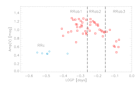
Figure 1: Bailey diagram ($V$-band amplitude versus logarithmic period) for the RRLs adopted to build the $V$-band light curve templates. The RRc variables are marked with blue circles and the RRab variables with red squares. The template bins are labeled and the period thresholds are displayed as vertical dashed lines.

We normalized all the light curves by subtracting the mean magnitude and dividing them by their peak-to-peak amplitude $A(V)$, and estimated $T_{mean}^{opt}$  and $T_{max}^{opt}$  for the entire sample and the individual values are listed in columns 5 and 6 of Table LABEL:tab:tmeantmax. $T_{mean}^{opt}$  was estimated as described in Appendix C.1 and $T_{max}^{opt}$  was estimated by converting the phase of maximum light of the model light curve, into an Heliocentric Julian Date.

Table 1: Photometric properties of the RRLs adopted to evaluate the optical light curve template. From left to right, the columns give the ID of the variable, the pulsation period, the mean visual magnitude, the $V$-band amplitude and the two reference epochs.

Name	Period	$<V>$	$Amp(V)$	$T_{mean}^{opt}$	$T_{max}^{opt}$
	(days)	(mag)		HJD-2,400,000 (days)
—RRc—
$\omega$ Cen  V16	0.3301961	14.558	0.487	51766.7639	51766.5041
$\omega$ Cen  V19	0.2995517	14.829	0.442	49869.6627	55715.4767
$\omega$ Cen  V98	0.2805656	14.773	0.461	55715.6665	51693.5392
$\omega$ Cen  V117	0.4216425	14.444	0.435	51277.1910	50985.5294
$\omega$ Cen  V264	0.3213933	14.703	0.430	54705.4664	52743.7623
M4 V6	0.3205151	13.454	0.434	55412.8765	49469.6457
M4 V43	0.3206600	13.082	0.430	43724.9882	43681.1370
—RRab1—
$\omega$ Cen  V8	0.5213259	14.671	1.263	49824.5018	52443.1571
$\omega$ Cen  V23	0.5108703	14.821	1.079	49866.6429	54705.6430
$\omega$ Cen  V59	0.5185514	14.674	0.907	51277.1348	51370.5255
$\omega$ Cen  V74	0.5032142	14.620	1.208	55711.7447	55715.3000
$\omega$ Cen  V107	0.5141038	14.753	1.169	49860.6035	53865.5023
M4 V2	0.5356819	13.411	0.965	55412.1842	52087.7853
M4 V7	0.4987872	13.415	1.061	55412.2209	50601.4511
M4 V8	0.5082236	13.323	1.108	55412.5025	50601.6924
M4 V10	0.4907175	13.327	1.251	55412.2533	50601.2890
M4 V12	0.4461098	13.578	1.272	55412.7833	50601.5210
M4 V16	0.5425483	13.344	0.893	55412.2979	50601.5688
M4 V18	0.4787920	13.358	1.121	55412.8648	50601.5170
M4 V19	0.4678111	13.376	1.237	55412.3131	50601.3741
M4 V21	0.4720074	13.190	1.127	55412.6133	50601.4735
M4 V26	0.5412174	13.247	1.235	55412.4631	50552.3694
M4 V36	0.5413092	13.424	0.921	55412.8657	52088.7312
M4 C303	0.4548026	16.037	1.232	55412.5626	50601.6896
AR Per	0.4255489	10.452	0.938	47123.6655	46773.4731
AV Peg	0.3903912	10.452	0.938	47123.7076	47116.3202
BB Pup	0.4805437	10.492	1.022	47193.3909	47193.4293
DX Del	0.4726174	10.492	1.022	43689.8611	30950.5060
SW And	0.4422660	12.164	0.976	47065.7327	47116.1847
V445 Oph	0.3970227	12.164	0.976	46981.3385	46868.6233
V Ind	0.4796012	9.937	0.704	47815.0317	47812.6680
—RRab2—
$\omega$ Cen  V13	0.6690484	14.471	0.959	51316.5671	51314.6124
$\omega$ Cen  V33	0.6023333	14.538	1.177	51285.7634	52446.5015
$\omega$ Cen  V40	0.6340978	14.511	1.121	49863.7202	54705.7382
$\omega$ Cen  V41	0.6629338	14.505	0.983	52743.9786	52447.0363
$\omega$ Cen  V44	0.5675378	14.709	0.975	50971.6089	50971.6529
$\omega$ Cen  V46	0.6869624	14.501	0.952	49821.6201	55715.8201
$\omega$ Cen  V51	0.5741424	14.511	1.178	51276.8553	50984.6520
$\omega$ Cen  V62	0.6197964	14.423	1.123	50984.4926	53860.3888
$\omega$ Cen  V79	0.6082869	14.596	1.164	49922.5029	50165.8572
$\omega$ Cen  V86	0.6478414	14.509	1.001	50978.5945	52743.3654
$\omega$ Cen  V100	0.5527477	14.638	1.028	50975.6290	50975.6676
$\omega$ Cen  V102	0.6913961	14.519	0.933	50975.5249	53864.9282
$\omega$ Cen  V113	0.5733764	14.596	1.250	50978.5866	52743.4734
$\omega$ Cen  V122	0.6349212	14.520	1.091	54705.4856	53870.6116
$\omega$ Cen  V125	0.5928780	14.587	1.202	49116.6901	51600.8905
$\omega$ Cen  V139	0.6768713	14.324	0.843	50972.5424	51276.5148
M4 V9	0.5718945	13.303	1.114	55412.7595	50601.4580
M4 V27	0.6120183	13.214	0.911	55412.7165	50601.6926
—RRab3—
$\omega$ Cen  V3	0.8412616	14.391	0.761	52743.3051	55715.5717
$\omega$ Cen  V7	0.7130342	14.594	0.950	49082.5766	49191.0218
$\omega$ Cen  V15	0.8106543	14.368	0.724	54705.5137	54705.6080
$\omega$ Cen  V26	0.7847215	14.470	0.618	50978.6516	54705.3909
$\omega$ Cen  V57	0.7944223	14.469	0.597	51766.3964	49876.5654
$\omega$ Cen  V109	0.7440992	14.426	0.995	50984.5494	52743.6624
$\omega$ Cen  V127	0.8349918	14.341	0.591	54705.2972	50984.6784
$\omega$ Cen  V268	0.8129334	14.544	0.467	51305.5583	2451336.5593

Note. — Tha table lists a few RRLs in common with those used for the RVC template. Periods might be slightly different, because we adopted different datasets for these two analyses.

Table 2: Coefficients and standard deviations of the PEGASUS fits to the $V$-band light curve template.

Template bin	N	$A_{0}$	$A_{1}$	$\phi_{1}$	$\sigma_{1}$	$A_{2}$	$\phi_{2}$	$\sigma_{2}$	$A_{3}$	$\phi_{3}$	$\sigma_{3}$	$A_{4}$	$\phi_{4}$	$\sigma_{4}$	$A_{5}$	$\phi_{5}$	$\sigma_{5}$
			$A_{6}$	$\phi_{6}$	$\sigma_{6}$	$A_{7}$	$\phi_{7}$	$\sigma_{7}$	$A_{8}$	$\phi_{8}$	$\sigma_{8}$	$A_{9}$	$\phi_{9}$	$\sigma_{9}$				$\sigma$
RRc ($T_{mean}^{opt}$)	8387	–0.5307	1.5916	8.0136	0.2750	–0.9843	0.5681	2.4905	–3.0543	0.0136	0.2443	1.8137	0.6700	1.1791	1.4625	0.0107	0.2233
			0.4535	–0.1160	0.5254	…	…	…	…	…	…	…	…	…				0.049
RRab1 ($T_{mean}^{opt}$)	25956	–0.0537	0.0241	2.4686	–0.3268	–0.4234	0.1043	0.5060	–0.6608	0.0204	0.2749	0.2908	0.6227	0.6791	0.3389	–0.0153	–0.1522
			0.9761	–0.0829	0.4306	–0.4576	–0.1291	0.2920	…	…	…	…	…	…				0.035
RRab2 ($T_{mean}^{opt}$)	26029	–0.3753	0.5372	3.5621	0.9021	–0.4391	0.0470	0.1680	–0.1191	0.0124	0.0657	0.1553	0.7271	0.3803	0.0485	0.0239	–0.0506
			0.6073	–0.0445	0.5040	–0.2475	0.0976	0.2170	–0.2263	0.1454	0.3674	…	…	…				0.028
RRab3 ($T_{mean}^{opt}$)	9787	–2.3494	–0.6802	4.0938	0.3433	–0.4498	0.2080	0.4693	–0.2342	0.0167	0.1190	0.6038	0.5839	0.7883	–0.0828	0.0854	0.1449
			2.8333	0.0219	1.5893	…	…	…	…	…	…	…	…	…				0.036
RRc ($T_{max}^{opt}$)	8387	–4.7750	–0.6122	2.8134	0.5686	0.0666	0.6401	0.2090	3.5226	0.0897	0.4441	–3.9216	1.0871	0.4602	5.4369	–0.3928	3.0508
			…	…	…	…	…	…	…	…	…	…	…	…				0.069
RRab1 ($T_{max}^{opt}$)	25956	–0.4586	–0.5500	1.1767	0.4577	0.0221	0.8182	–0.1123	–1.5880	0.9838	0.4772	0.9760	0.9329	0.3396	–0.2869	1.3225	0.4907
			–0.4888	–1.0239	–0.1842	1.3798	1.0799	–1.3487	…	…	…	…	…	…				0.043
RRab2 ($T_{max}^{opt}$)	26029	0.4326	0.3797	0.5056	2.2368	–1.3584	–0.0486	1.3392	–2.8021	0.0117	0.2499	0.4585	0.7517	0.7523	2.1228	0.0195	0.2295
			0.7873	–0.0764	0.4384	…	…	…	…	…	…	…	…	…				0.035
RRab3 ($T_{max}^{opt}$)	9787	–1.5356	–0.2273	1.0032	0.3180	0.1744	0.7173	0.5384	–0.0470	–0.0120	0.0916	1.7028	0.5273	1.7784	0.3626	0.7872	0.3318
			0.1686	–0.1563	0.1623	…	…	…	…	…	…	…	…	…				0.055

We visually inspected all the reference epochs derived in this work (see Figure 2). To overcome thorny problems in the phasing of light curves, we manually selected the best value of $T_{max}^{opt}$  as the HJD of the phase point closest to the maximum for the variables where the fit does not follow closely the data around maximum light. In contrast, no manual selection of $T_{mean}^{opt}$  was needed because its estimation is, by its own nature, based on a more robust approach. We anchored the phases to both $T_{max}^{opt}$  and $T_{mean}^{opt}$  and we piled up the light curves into four period bins. We ended up with eight cumulative and normalized light curves: four with $\tau_{0}$ anchored to $T_{max}^{opt}$  and four anchored to $T_{mean}^{opt}$.

Finally, we adopted the PEGASUS (PEriodic GAuSsian Uniform and Smooth) function (a series of multiple periodic Gaussians, Inno et al. 2015) to fit the cumulative and normalized light curves. The form of the PEGASUS fit is:

$$P(\phi)=A_{0}+\Sigma_{i}A_{i}\exp{\Big{(}-\sin{\Big{(}\dfrac{\pi(\phi-\phi_{i})}{\sigma_{i}}\Big{)}^{2}}\Big{)}}$$ (1)

where $A_{0}$ and $A_{i}$ are the zero points and the amplitudes of the Gaussians, while $\phi_{i}$ and $\sigma_{i}$ are the centers and the $\sigma$ of the Gaussians.

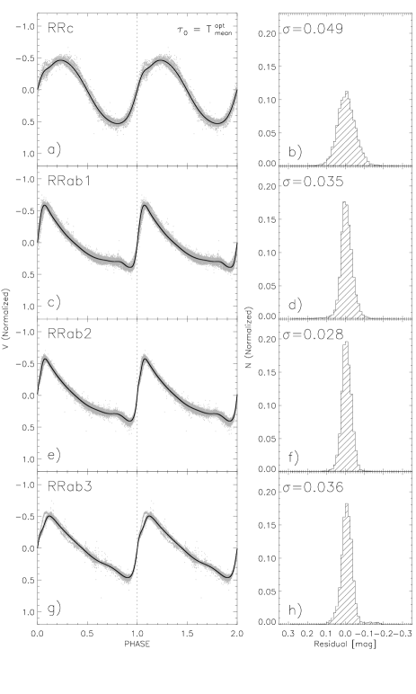
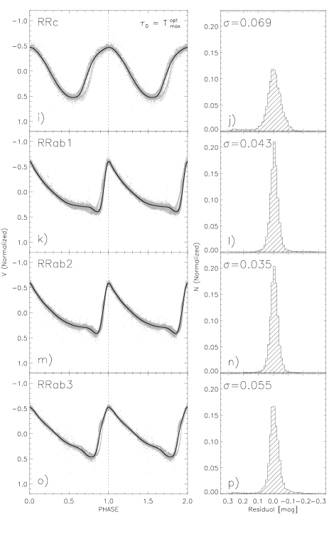
Figure 2: Panels a) to h): the left panels—a), c), e) and g)—display, from top to bottom, cumulative and normalized $V$-band light curves for the four different period bins phased by assuming as reference epoch $\tau_{0}$=$T_{mean}^{opt}$. The individual measurements are marked with light grey dots, while the black solid line shows the analytic fit of the light curve template and the vertical dotted line the reference epoch. The right panels—b), d), f) and h)—display the histogram of the residuals of individual phase points with respect to the analytical fit. The standard deviations of the distribution of the residuals are also labeled. Panels i) to p): Same as a) to h), but the $V$-band light curves were phased by assuming as reference epoch $\tau_{0}$=$T_{max}^{opt}$.

Figure 2 displays the cumulative and normalized light curves of the four period bins. The black solid lines plotted in left and right panels show the analytical fits of the cumulative and normalized $V$-band light curves with PEGASUS functions (see Eq. 2). The coefficients of the PEGASUS fits are listed in Table 2. The standard deviations plotted to the right of the light curves (see also the last column in Table 2) bring forward two interesting results. i)– The standard deviations of the light curves phased by using $T_{mean}^{opt}$  are systematically smaller than those phased using $T_{max}^{opt}$. The difference for the period bins in which the light curves display a cuspy maximum (RRab1, RRab2) is $\sim$37% smaller, but it becomes $\sim$45% smaller for the RRc and the RRab3 period bins, because they are characterized by flat-topped light curves. ii)– The cumulative light curves for the RRc and RRab3 period bins phased using $T_{max}^{opt}$  show offsets along the rising branch. This mismatch could lead to systematic offsets of $\sim$30% in $Amp(V)$ adopted to estimate the mean $<V>$ magnitude. Meanwhile, the cumulative light curves phased using $T_{mean}^{opt}$  overlap better with each other over the entire pulsation cycle. There is one exception: the RRab3 period bin shows a marginal difference across the phases of maximum in luminosity, but the error in the adopted $Amp(V)$ is on average a factor of two smaller ($\sim$15%) than those obtained by using $T_{max}^{opt}$  as anchor.

The current circumstantial evidence, based on the same photometric data, indicates that the use of a reference epoch anchored to the phase of mean magnitude along the rising branch allows a more accurate phasing with respect to the phase of the maximum in luminosity.

2.2 Phase offset between $T_{max}^{opt}$  and $T_{mean}^{opt}$

We are aware that large photometric surveys—but also smaller projects focused on variable stars—provide, as reference epoch, $T_{max}^{opt}$. To overcome this difficulty and to provide a homogeneous empirical framework, we investigated the phase offset between $T_{mean}^{opt}$  and $T_{max}^{opt}$. In particular, we defined the phase difference

$$\Delta\Phi=\dfrac{(T_{max}^{opt}-T_{mean}^{opt})}{P}\bmod{1}$$

where $\bmod$ is the remainder operator. For this purpose, we could adopt a larger sample of visual light curves of 291 RRLs (54 RRc and 237 RRab) from large photometric surveys (Gaia, ASAS, ASAS-SN and Catalina), from our own photometry of globular clusters ($\omega$ Cen, M4), and from the literature (BW sample, see caption of Table 11). We found that the phase difference shows, as expected, a trend with the pulsation period (see Figure 3).

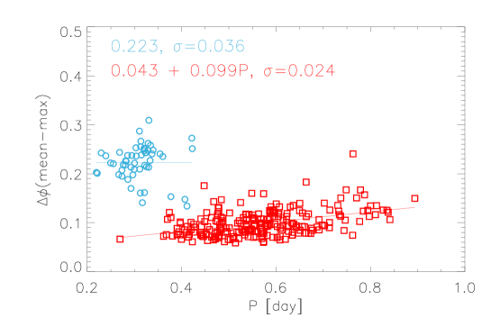
Figure 3: $V$-band $\Delta\Phi$ versus pulsation period for RRc (blue) and RRab (red) variables. The constant offset for RRc variables and the linear relation for RRab variables are displayed as solid lines. The offset and the linear relation are labeled at the top-left corner together with their standard deviations.

In particular, the RRab variables show a quite clear linear trend of phase offset with period ($\Delta\Phi=0.043+0.099\cdot P$), with an intrinsic dispersion of 0.024. The standard deviation for RRc variables is larger, but there is no clear sign of a period dependency. Therefore, we assume a constant phase difference ($\Delta\Phi=$0.223$\pm$0.036) for RRc variables. We also investigated a possible correlation of phase offset with metallicity by adopting the estimates recently provided by Crestani et al. (2021a), but we found none.

3 Radial velocity database

To provide new RVC templates we performed a large spectroscopic campaign aimed at providing RV measurements for both field and cluster RRLs. We reduced and analyzed a large sample of high-, medium- and low-resolution (HR, MR, LR) spectra. This mix of proprietary data and data retrieved from public science archives was supplemented with RVCs of RRLs available in the literature.

3.1 Spectroscopic catalog

We collected the largest spectroscopic dataset—both proprietary and public—for RRLs. Preliminary versions of this spectroscopic catalog were already used in studies focused on chemical abundances (Fabrizio et al. 2019; Crestani et al. 2021a, b) and RV (Bono et al. 2020a). In this investigation, we added new spectroscopic data and discuss in detail the spectra used for RV measurements. We ended up with 23,865 spectra for 10,413 RRLs. Figure 4 shows that the distribution of the RRLs is well-spread over the Galactic Halo. The key properties of the spectra (spectral resolution and signal-to-noise ratio), the spectrographs and the spectroscopic sample are summarized in Table 3.

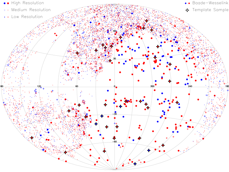
Figure 4: Aitoff projection in Galactic coordinates ($l,b$) of the RRL spectroscopic dataset. Blue and red symbols display RRc and RRab variables. High-, medium-, and low-resolution spectra are marked with large circles, crosses, and small circles, respectively. RRL for which we only have radial velocity measurements from the literature are plotted as diamonds (Baade-Wesselink sample, see Section 4.2). Black stars indicate the RRLs used to build the RVC templates.

Table 3: Key properties of the different spectroscopic datasets adopted in this investigation.

Instrument	Nspectra	NRRab	NRRc	R	SNR
—High resolution—
du Pont	6208	114	76	35,000	40
FEROS@2.2m	55	3	0	48,000	13
HARPS-N@TNG	10	0	4	115,000	40
HARPS@3.6m	320	19	6	115,000	10
HRS@SALT	81	64	5	40,000	50
SES@STELLA	100	0	8	55,000	35
HDS@Subaru	34	23	2	60,000	35
UVES@VLT	277	62	8	34,540-107,200	20
—Medium resolution—
X-Shooter@VLT	121	16	2	4,300–18,000	45
LAMOST-MR	1271	106	66	7,500	22
—Low resolution—
LAMOST-LR	9099	4275	1935	2,000	22
SEGUE-SDSS	5110	2487	1197	2,000	21
—Total—
	23865	7070	3343

Note. — Each row gives either the spectrograph or the spectroscopic dataset (column 1), the total number of spectra (column 2), the number of RRab and RRc variables (column 3 and 4), the typical spectral resolution (column 5) and the typical SNR@3950 $\;\buildrel\circ\over{\rm A}$(column 6).

The HR sample mainly includes spectra collected with the Las Campanas Observatory du Pont echelle spectrograph (du Pont, 6,208 spectra), plus HR spectra collected from ESO telescopes (277 from UVES@VLT, 320 from HARPS@3.6m, 55 from FEROS@2.2m MPG). We also have 100 HR spectra from SES@STELLA, 81 from HRS@SALT, 10 from HARPS-N@TNG and 34 from HDS@Subaru. We collected MR spectra from both X-Shooter@VLT (121 spectra) and the LAMOST MR survey (1271 spectra). Finally, our spectroscopic dataset includes LR spectra from the LAMOST (9,099 spectra) and from the SDSS-SEGUE (6,289 spectra) surveys.

4 Radial velocity curves

The main aim of this investigation is to provide RVC templates that can be used to provide V_γ for RRLs from a few random RV measurements based on a wide variety of spectra. For this purpose, we selected a broad range of strong and weak spectroscopic diagnostics.

4.1 Radial velocity spectroscopic diagnostics

The decision to use multiple spectroscopic diagnostics was made because different lines form at different atmospheric layers. As the RRL are pulsating stars, different lines may trace very different kinematics even when observed at the same phase. The resulting velocity curves for different lines, therefore, may have different shapes and amplitudes. Consequently, combining different hydrogen and/or metallic lines for a single velocity determination would blur the fine detail of the velocity curves and decrease the accuracy of the V_γ estimate. With this in mind, we performed RV measurements separately with the following diagnostics: four Balmer lines (H_α, H_β, H_γ and H_δ), the Na doublet (D1 and D2), the Mg I b triplet (Mg b₁, Mg b₂ and Mg b₃) and a set of Fe and Sr lines (three lines of the Fe I multiplet 43 and a resonant Sr II line, Moore 1972).

The laboratory wavelengths of the quoted absorption lines are listed in Table 4. Figure 5 displays the regions of the spectrum of four RRLs where the quoted lines are located. The four RRLs were selected in order to have one RRL for each period bin of the RVC template (see Section 4.4). To measure the RVs for the quoted diagnostics we performed a Lorentian fit to the absorption lines by using an automated procedure written in IDL. The wavelength range adopted by the fitting algorithm is fixed according to the spectral resolution of the different spectrographs. Typically, we selected a range in wavelength that is ten Full Width at Half Maximum (FWHM) to the left and ten to the right. The FWHM was estimated as FWHM=$2.355\times\dfrac{\lambda_{obs}}{R}$, where $\lambda$ is the wavelength of the diagnostic and R is the spectral resolution.

Table 4: Wavelengths of the lines adopted for radial velocity measurements.

Species	Line ID	$\lambda$ [$\;\buildrel\circ\over{\rm A}$]
—Balmer lines—
Hα	Hα	6562.80
Hβ	Hβ	4861.36
Hγ	Hγ	4340.46
Hδ	Hδ	4101.74
—Fe group—
Fe I	Fe1	4045.81
Fe I	Fe2	4063.59
Fe I	Fe3	4071.74
Sr II	Sr	4077.71
—Mg group—
Mg I	Mg b1	5167.32
Mg I	Mg b2	5172.68
Mg I	Mg b3	5183.60
—Na group—
Na I	D1	5889.95
Na I	D2	5895.92

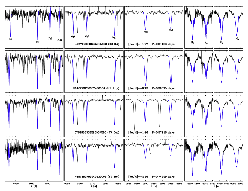
Figure 5: From top to bottom, HR spectra collected with du Pont for RRLs adopted in the four bins of the RVC template. The flux units are arbitrary. The Gaia ID (alternative name in parentheses), iron abundance ([Fe/H]) and the pulsation period are labeled. The four portions of the spectrum display, from left to right, the metallic lines, Mg I b triplet, Na doublet and the Balmer lines. Each line is marked in blue and labeled. All the spectra presented in this figure were taken at phases near one third of the rising branch of the RV curve and are only minimally affected by nonlinear phenomena. The first row shows the spectrum of the RRc variable CS Eri. Second row: same as the top, but for the RRab HH Pup. Third row: same as the top but, for the RRab RV Oct. Fourth row: same as the top but, for the RRab AT Ser.

The median uncertainties of the single RV estimates for the adopted spectroscopic diagnostics and the standard deviations of the different datasets are listed in Table 5. Note that the different datasets have median uncertainties, on average, smaller than 1.5 km/s.

Table 5: Typical uncertainties in radial velocity measurements for the adopted diagnostics in the different spectroscopic datasets.

	eRV(Fe)		eRV(Mg)		eRV(Na)		eRV(Hα)		eRV(Hβ)		eRV(Hγ)		eRV(Hδ)
Instrument	mdn	$\sigma$	mdn	$\sigma$	mdn	$\sigma$	mdn	$\sigma$	mdn	$\sigma$	mdn	$\sigma$	mdn	$\sigma$
	(km/s)		(km/s)		(km/s)		(km/s)		(km/s)		(km/s)		(km/s)
—High resolution—
du Pont	0.168	2.154	0.217	1.592	0.382	0.257	0.966	0.488	0.944	0.510	1.168	1.173	1.200	1.446
FEROS@2.2m	0.145	0.023	0.166	0.028	0.161	0.033	1.027	0.162	0.819	0.130	1.008	0.110	0.991	0.063
HARPS-N@TNG	0.094	0.032	0.133	0.030	0.160	0.033	0.938	0.119	0.923	0.090	1.010	0.088	1.037	0.110
HARPS@3.6m	0.180	0.054	0.203	0.059	0.160	0.154	1.238	0.246	0.897	0.558	1.106	0.648	1.045	0.613
HRS@SALT	0.209	2.186	0.214	0.811	0.229	0.270	1.181	0.407	1.105	0.387	1.851	0.742	2.948	2.174
SES@STELLA	0.329	1.094	0.178	0.411	0.000	1.491	0.808	3.193	0.677	0.278	0.785	1.323	0.801	1.379
HDS@Subaru	…	…	0.185	0.028	0.200	0.071	0.790	0.192	…	…	…	…	…	…
UVES@VLT	0.167	0.041	0.196	0.047	0.219	0.075	1.089	0.344	0.912	0.252	1.106	0.218	1.045	0.358
—Medium resolution—
X-Shooter@VLT	0.259	0.003	0.329	0.011	0.263	0.136	1.189	0.232	1.071	0.181	1.106	0.100	1.045	0.039
LAMOST-MR	0.259	0.058	0.329	0.046	0.375	0.129	1.494	0.410	1.239	0.221	1.106	0.168	1.045	0.095
—Low resolution—
LAMOST-LR	2.863	1.495	3.657	1.214	4.168	1.874	4.645	1.182	3.440	0.528	3.072	0.421	1.983	0.492
SEGUE-SDSS	…	…	…	…	…	…	4.180	0.572	3.096	0.411	2.765	0.331	2.613	0.209

Note. — Medians (mdn) and standard deviations ($\sigma$) of the uncertainties on the RV measurements for the Fe, Mg, Na, H_α, H_β, H_γ and H_δ lines

4.2 Radial velocity curves from the literature

To complement our dataset, we collected RVCs of RRLs from the literature (Liu & Janes 1989; Skillen et al. 1993b, a; Jones et al. 1988a, b; Cacciari et al. 1987; Jones et al. 1987a; Clementini et al. 1990; Fernley et al. 1990; Jones et al. 1987b). During the 80s and 90s of the previous century, several bright RRLs were observed both photometrically (optical and NIR) and spectroscopically (velocities from metallic lines) to apply the Baade-Wesselink method (BW, Baade 1926; Wesselink 1946) in order to obtain accurate distance determinations. Therefore, we label the set of RVCs from these works as the BW sample. Unfortunately, it was not possible to collect the spectra, therefore we adopted the RV estimates as provided in the quoted papers. Overall, the BW sample includes 2,725 RV measurements for 36 RRab and 3 RRc.

Although this dataset is inhomogeneous and based on a mix of weak metallic lines, it is extremely useful to complement our own measurements. Some of the works mentioned above included optical light curves, which we used to validate the robustness of the reference epoch used in the phasing of the RVC template.

4.3 Estimate of barycentric velocities, radial velocity amplitudes and reference epochs

To derive the analytic form of the RVC templates, it is necessary to know the pulsation period (P), the reference epoch, $V_{\gamma}$ and the RV amplitude ($Amp(RV)$) of the RRLs with a well-sampled RV curve. The former two are needed to convert epochs into phases and the latter two are used for the normalization of the RV curve. The normalization is a crucial step because the RVC templates have to be provided as normalized curves, with zero mean and unit amplitude.

Our data set includes RV measurements for more than 10,000 RRLs, but only 74 of them have a well-sampled pulsation cycle. A good phase coverage is necessary for the determination of the pulsation properties required for the creation of the RVC template. Reference epochs and $Amp(RV)$ are particularly sensitive to the quality of the pulsation cycle sampling. We neglected all the RRLs displaying a clear Blazhko effect (a modulation of the pulsation amplitude, both in light and in RV) that would introduce a large intrinsic spread in the RVC templates. Because of this exacting quality control, we derived the analytic form of the RVC template using only a subset of three dozen RRL in the spectroscopic template (31 RRab, 5 RRc). They cover a broad range in pulsation periods (0.27-0.84 days) and iron abundances (–2.6 $\leq$ [Fe/H]$\leq$–0.2). We label these stars with the name “Template Sample” (TS) and their properties are listed in Table 6. The individual RV measurements for the TS variables are given in Table 7.

Table 6: Calibrating RRLs used to derive the RVC templates. From left to right the columns list the Gaia EDR3 ID, the alternative ID, pulsation period, mean visual magnitude, visual amplitude, reference epochs ($T_{mean}^{RV}$  and $T_{min}^{RV}$, both for Fe and H_β RVCs), iron abundance and its error.

Gaia EDR3 ID	name	Period	$V$	$Amp(V)$	$T_{mean}^{RV(Fe)}$	$T_{min}^{RV(Fe)}$	$T_{mean}^{RV(H\beta)}$	$T_{min}^{RV(H\beta)}$	[Fe/H]	e[Fe/H]
		(days)	(mag)		HJD-2,400,000 (days)
—RRc—
6884361748289023488	YZ Cap	0.2734529	11.275	0.490	55461.3137	55461.3460	58320.2616	58320.0357	–1.50	0.02
6856027093125912064	ASAS J203145-2158.7	0.3107106	11.379	0.370	56915.4305	56915.1735	56915.1343	56915.1813	–1.17	0.03
4947090013255935616	CS Eri	0.3113302	8.973	0.520	56919.7069	56919.4373	56919.3975	56919.4442	–1.89	0.02
6662886605712648832	MT Tel	0.31689945	8.962	0.560	56919.3010	56919.3476	58574.4677	58574.5252	–2.58	0.03
5022411786734718208	SV Scl	0.3773586	11.350	0.530	56916.2869	56916.3304	56916.2943	56916.3480	–2.28	0.04
—RRab1—
1793460115244988800	AV Peg	0.3903809	10.561	1.022	56531.4845	56531.1300	56531.0981	56531.1245	–0.18	0.10
5510293236607430656	HH Pup	0.3908119	11.345	1.240	55962.2982	58472.9012	58472.8823	55959.5915	–0.93	0.15
4352084489819078784	V0445 Oph	0.397026	10.855	0.810	56530.9768	56531.0228	56530.9811	56531.0078	–0.01	0.15
3652665558338018048	ST Vir	0.41080754	11.773	1.180	56468.9303	56468.9685	58322.4995	58322.5333	–0.86	0.15
3546458301374134528	W Crt	0.4120119	11.517	1.294	56076.2014	56076.2294	58620.7984	58620.8240	–0.75	0.15
4467433017738606080	VX Her	0.4551803	10.791	1.200	56472.1573	57880.9753	57880.9507	57880.9885	–1.42	0.17
2689556491246048896	SW Aqr	0.4593007	11.199	1.281	56175.1772	56175.2107	56175.1868	55815.5797	–1.38	0.15
1760981190300823808	DX Del	0.47261773	9.898	0.700	56472.2987	56472.3478	56472.3059	56472.3422	–0.40	0.10
3698725337376560512	UU Vir	0.47560267	10.533	1.127	56471.7854	56471.8215	58573.9638	58574.0025	–0.81	0.10
6771307454464848768	V0440 Sgr	0.4775	10.269	1.101	54305.4643	54305.0241	54304.9903	54305.0308	–1.15	0.10
3915998558830693888	ST Leo	0.47797595	11.585	1.190	56466.8416	56466.8722	56466.8559	56466.8884	–1.31	0.15
6483680332235888896	V Ind	0.47959915	9.920	1.060	57620.0005	57620.0375	57620.0144	57620.0519	–1.46	0.14
1191510003353849472	AN Ser	0.52207295	10.922	1.010	56468.9009	57880.6326	57880.5948	57880.6280	–0.05	0.15
—RRab2—
2558296724402139392	RR Cet	0.55302505	9.704	0.938	56171.2955	56171.3458	56171.3170	56171.3585	–1.41	0.03
3479598373678136832	DT Hya	0.5679814	13.042	0.940	54583.0190	54583.0673	54583.0367	54583.0872	–1.43	0.10
6570585628216929408	TY Gru	0.57006515	14.104	0.950	55820.0694	55820.1104	55820.0923	54690.8307	–1.99	0.10
5769986338215537280	RV Oct	0.571178	10.954	1.130	54690.3296	54689.8001	54689.7797	54689.8224	–1.50	0.10
5412243359495900928	CD Vel	0.57350788	12.000	0.870	54908.3154	54907.7975	54907.7630	54907.8141	–1.78	0.10
5461994302138361728	WY Ant	0.57434364	10.773	0.850	54903.8161	58617.5685	58617.5474	58617.5909	–1.88	0.10
5806921716937210496	BS Aps	0.5825659	12.155	0.680	55644.5855	55644.0827	55644.0232	55644.0810	–1.49	0.10
6787617919184986496	Z Mic	0.58692775	11.489	0.640	57287.6695	58306.0549	58306.0075	58306.0631	–1.51	0.10
5773390391856998656	XZ Aps	0.58726739	12.285	1.100	55018.9886	55019.0308	55019.0114	55019.0660	–1.78	0.10
4860671839583430912	SX For	0.6053453	11.077	0.640	56529.0510	56529.1188	58061.8060	58061.8531	–1.80	0.15
3797319369672686592	SS Leo	0.62632619	11.034	1.152	58247.1761	58246.6024	58246.5755	58246.6350	–1.91	0.07
2381771781829913984	DN Aqr	0.63376712	11.139	0.720	57261.0936	57261.1589	57261.1112	57261.1760	–1.76	0.15
4709830423483623808	W Tuc	0.64224028	11.429	1.178	56528.8863	56528.9377	58062.5835	55457.7106	–1.76	0.15
15489408711727488	X Ari	0.65117537	9.583	0.940	56531.5437	56530.9654	58394.5863	58394.6450	–2.52	0.17
—RRab3—
1360405567883886720	Cl* NGC 6341 SAW V1	0.70279828	15.059	0.986	48054.4181	48053.7930			–2.38	0.07
4417888542753226112	VY Ser	0.7141	10.065	0.675	56468.5381	54574.8381	58654.4207	58654.4811	–1.82	0.10
4454183799545435008	AT Ser	0.74655408	11.463	0.890	56530.9316	56530.2582	58326.4245	58326.4957	–2.05	0.22
6701821205809488384	ASAS J181215-5206.9	0.8375398	13.258	0.480	55328.2311	55017.5992	55327.4451	55327.5812	…	…

Table 7: Individual radial velocity measurements for the calibrating RRLs. From left to right the different columns list the name of the variable, the spectroscopic diagnostic, heliocentric Julian date, the radial velocity, the error on the radial velocity and the spectrograph.

Name	Species	HJD	RV	eRV	Instrument
		(days)	(km/s)
CS Eri	Fe	2456919.6422	–133.915	0.767	du Pont
CS Eri	Fe	2456919.6475	–133.843	1.496	du Pont
CS Eri	Fe	2456919.6528	–133.221	0.896	du Pont
CS Eri	Fe	2456919.6582	–133.492	0.884	du Pont
CS Eri	Fe	2456919.6635	–133.689	0.896	du Pont
CS Eri	Fe	2456919.6689	–134.396	0.985	du Pont
CS Eri	Fe	2456919.6761	–136.157	0.888	du Pont
CS Eri	Fe	2456919.6815	–136.982	0.889	du Pont
CS Eri	Fe	2456919.6868	–138.586	0.805	du Pont
CS Eri	Fe	2456919.6921	–139.538	0.517	du Pont

Note. — Only ten lines are listed. The machine-readable version of this table is available online on the CDS.

The RRLs in the TS have well-covered RVCs for all the adopted spectroscopic diagnostics. The only exception is a cluster star (Cl* NGC 6341 SAW V1) that has good RVCs only for Fe and Mg lines. The number of calibrating RRLs adopted in this work is six times larger than the RRL sample adopted by S12. Moreover, S12 only included RRab variables covering a limited range in pulsation periods (0.56-0.59 days).

To estimate $V_{\gamma}$, $Amp(RV)$, the epoch of mean velocity on the decreasing branch and the epoch of minimum velocity ($T_{mean}^{RV}$  and $T_{min}^{RV}$, both for Fe and H_β RVCs), we fitted the RVCs with the PLOESS algorithm, as described in Bono et al. (2020a). Then, we derived $V_{\gamma}$ as the average of the fit and $Amp(RV)$ as the difference between the maximum and the minimum of the fit. The estimates of $V_{\gamma}$, $Amp(RV)$ and their uncertainties are provided in Tables 8 and 9. Note that we provide these estimates for both the Balmer lines and for the averaged RVCs of Fe, Na and Mg. By using $V_{\gamma}$ and $Amp(RV)$, we normalized all the RVCs of the TS RRLs and derived the Normalized RVCs (NRVCs).

Table 8: Barycentric radial velocities and RV amplitudes based on Balmer lines.

Name	Hα				Hβ				Hγ				Hδ
	$V_{\gamma}$	e$V_{\gamma}$	$Amp(RV)$	e$Amp(RV)$	$V_{\gamma}$	e$V_{\gamma}$	$Amp(RV)$	e$Amp(RV)$	$V_{\gamma}$	e$V_{\gamma}$	$Amp(RV)$	e$Amp(RV)$	$V_{\gamma}$	e$V_{\gamma}$	$Amp(RV)$	e$Amp(RV)$
	(km/s)				(km/s)				(km/s)				(km/s)
YZ Cap	–107.17	1.48	37.09	3.16	–109.37	1.56	29.56	2.90	–112.82	2.09	29.29	2.84	–105.05	1.71	21.98	2.47
DR Cap	–1.66	1.18	30.42	2.94	–3.25	1.21	25.31	2.54	–1.83	1.82	25.25	2.94	–4.42	1.89	26.86	4.80
CS Eri	–145.11	1.02	48.15	3.79	–146.63	1.12	35.14	2.96	–146.73	1.19	33.42	2.75	–142.83	1.24	28.58	2.61
MT Tel	65.64	1.10	35.65	2.26	64.23	1.15	27.37	1.94	65.26	1.21	25.80	1.91	66.87	1.29	22.03	1.81
SV Scl	–14.60	1.11	42.70	3.19	–15.94	1.21	32.64	2.73	–14.93	1.34	29.18	2.58	–11.09	1.56	23.17	2.48
AV Peg	–57.29	0.94	92.66	4.07	–62.00	0.98	72.66	3.27	–66.26	1.59	67.53	3.21	–59.05	1.55	59.07	2.98
HH Pup	18.11	1.02	110.28	4.30	17.05	1.02	86.75	3.74	15.65	1.33	80.19	3.29	20.66	1.21	70.89	2.98
V0445 Oph	–19.51	1.27	90.33	7.07	–24.41	1.18	68.82	5.16	–28.84	1.53	63.08	4.79	–21.29	1.62	58.15	4.98
ST Vir	–1.26	1.40	95.80	5.42	–4.63	1.54	73.00	4.24	–2.24	1.61	75.59	4.48	–3.03	1.57	61.47	3.81
W Crt	60.86	1.21	101.33	4.17	59.32	1.15	84.23	3.55	56.66	1.57	76.17	3.28	61.81	1.38	66.79	2.89
VX Her	–376.05	1.72	105.14	7.29	–376.92	1.85	80.88	6.88	–379.06	2.35	75.14	5.33	–373.62	2.01	57.18	4.06
SW Aqr	–49.20	1.08	103.54	4.13	–49.17	1.13	76.46	3.82	–49.25	1.36	80.24	3.42	–46.23	1.55	66.89	2.99
DX Del	–56.88	0.95	92.90	5.42	–60.81	0.98	71.37	3.92	–62.74	1.31	66.59	3.78	–58.20	1.19	58.22	3.24
UU Vir	–12.08	0.89	110.49	6.31	–12.51	0.93	94.20	5.79	–11.12	1.45	88.31	4.28	–9.62	1.28	75.87	3.53
V0440 Sgr	–64.10	1.67	98.91	6.24	–64.22	1.93	84.25	6.78	–60.83	1.96	74.25	5.63	–59.86	1.99	67.85	5.09
ST Leo	165.14	1.72	114.08	8.18	165.08	1.05	82.29	5.35	163.93	1.55	86.00	5.88	169.63	1.68	69.03	4.78
V Ind	200.88	0.95	101.31	3.39	200.31	0.85	78.22	2.58	201.52	1.04	73.88	2.48	203.00	0.95	61.37	2.07
AN Ser	–41.71	1.35	95.50	6.29	–44.51	1.50	73.11	4.87	–51.79	1.77	69.88	4.65	–42.15	1.55	57.87	3.77
RR Cet	–77.69	1.06	107.53	5.23	–77.19	1.28	82.88	4.13	–75.66	1.72	77.60	4.02	–73.85	1.42	72.01	3.67
DT Hya	75.15	1.30	110.59	5.82	77.66	1.12	82.92	4.23	77.45	1.43	81.03	4.31	82.13	1.46	71.75	3.87
TY Gru	–12.28	1.54	105.82	4.14	–11.13	1.69	80.50	3.24	–6.89	1.95	81.11	3.37	–8.79	2.19	63.10	3.13
RV Oct	137.23	1.42	104.50	3.63	139.60	1.15	85.93	3.00	141.51	1.35	85.52	3.12	144.78	1.29	75.42	2.86
CD Vel	239.70	0.95	96.88	3.86	240.15	0.83	77.77	3.02	241.53	1.11	74.63	2.95	243.02	1.07	62.65	2.52
WY Ant	201.31	0.93	108.83	5.62	202.26	0.78	84.27	4.27	204.58	1.00	76.90	4.12	206.15	0.99	67.96	3.45
BS Aps	–106.76	1.25	85.20	3.01	–108.88	1.08	65.30	2.28	–105.39	1.22	61.26	2.21	–103.51	1.36	56.18	2.22
Z Mic	–58.64	0.94	92.91	3.61	–61.08	0.79	74.78	2.88	–58.05	0.98	68.05	2.67	–57.44	1.05	60.64	2.41
XZ Aps	192.39	1.02	104.24	3.14	195.55	0.91	85.62	2.62	197.67	1.46	85.91	2.85	198.92	1.60	67.22	2.49
SX For	243.01	1.25	91.87	5.73	242.72	0.99	69.79	3.98	244.01	1.17	65.42	3.86	245.87	1.01	59.78	3.45
SS Leo	160.70	0.99	103.73	5.54	161.11	1.17	83.63	4.13	164.42	1.56	80.95	4.00	164.07	1.61	73.69	3.62
DN Aqr	–229.89	0.87	101.94	5.14	–228.68	0.84	83.05	4.38	–229.00	1.04	81.96	4.14	–225.74	1.31	64.72	3.50
W Tuc	56.91	1.07	114.34	5.36	59.96	0.99	85.68	4.10	63.23	1.20	82.03	3.88	65.48	1.15	69.92	3.41
X Ari	–41.58	1.08	109.64	4.40	–39.73	0.97	89.55	3.47	–37.97	1.27	77.70	3.10	–36.22	1.43	67.65	2.86
VY Ser	–147.44	0.95	97.31	10.27	–148.75	0.81	79.42	6.68	–146.66	0.94	70.92	5.80	–146.87	0.87	64.06	4.70
AT Ser	–71.38	1.00	102.45	7.35	–70.38	1.16	79.59	5.50	–68.68	1.42	79.90	5.60	–63.33	1.44	68.66	4.63
V0384 Tel	302.85	1.45	87.45	10.13	303.03	0.98	71.76	9.27	303.04	1.99	60.79	8.15	303.90	1.75	55.80	6.81

Note. — Note that Cl* NGC 6341 SAW V1 does not appear because the Balmer RV measurements for this star are not accurate.

Table 9: Barycentric radial velocities and RV amplitudes based on metallic lines.

Gaia DR2 ID	Fe				Mg				Na
	$V_{\gamma}$	e$V_{\gamma}$	$Amp(RV)$	e$Amp(RV)$	$V_{\gamma}$	e$V_{\gamma}$	$Amp(RV)$	e$Amp(RV)$	$V_{\gamma}$	e$V_{\gamma}$	$Amp(RV)$	e$Amp(RV)$
	(km/s)				(km/s)				(km/s)
YZ Cap	–109.60	0.16	26.34	1.09	–109.05	0.16	26.47	1.55	–109.05	0.41	27.76	2.33
DR Cap	–3.34	0.18	22.77	1.17	–2.19	0.20	23.00	1.72	–3.25	0.48	27.30	2.76
CS Eri	–145.25	0.12	29.08	1.21	–145.31	0.17	29.17	1.74	–145.60	0.39	31.43	2.61
MT Tel	66.43	0.14	22.82	0.73	65.98	1.17	22.99	1.90	65.32	0.71	23.19	1.53
SV Scl	–14.14	0.19	26.87	1.14	–13.98	0.17	26.80	1.56	–15.68	0.30	26.81	2.06
AV Peg	–60.48	0.28	63.52	1.41	–56.63	0.32	64.58	2.00	–55.89	0.69	68.71	3.06
HH Pup	18.59	0.21	69.27	1.36	19.65	0.29	71.16	1.95	19.00	0.65	71.42	2.82
V0445 Oph	–21.96	0.32	57.42	2.25	–18.57	0.44	57.16	2.98	–18.36	0.67	61.45	4.70
ST Vir	–4.52	0.27	60.60	1.74	–1.43	0.54	62.44	2.62	–2.50	0.64	66.75	3.83
W Crt	61.38	0.28	67.49	1.27	63.66	0.50	68.39	1.84	62.69	0.70	70.41	2.76
VX Her	–375.68	0.50	61.93	1.86	–374.55	0.65	62.76	2.62	–375.59	0.98	62.61	3.68
SW Aqr	–48.64	0.23	62.54	1.25	–47.21	0.30	62.31	1.72	–47.80	0.48	64.74	1.90
DX Del	–58.96	0.24	53.90	1.48	–55.69	0.54	54.27	2.05	–55.59	0.60	57.46	3.39
UU Vir	–11.15	0.20	67.45	1.46	–3.30	0.45	69.21	2.11	–8.80	0.62	69.22	3.07
V0440 Sgr	–60.99	0.48	63.10	2.60	…	…	…	…	–36.16	1.64	95.08	9.03
ST Leo	165.87	0.29	65.39	2.12	168.07	0.34	65.51	2.94	167.40	0.54	66.96	4.44
V Ind	201.04	0.16	56.09	0.83	201.86	0.25	56.48	1.24	201.17	0.42	57.87	1.39
AN Ser	–43.34	0.33	59.90	1.84	–39.68	0.54	60.80	2.56	–38.94	1.01	60.08	3.96
RR Cet	–75.49	0.18	61.77	1.62	–74.13	0.37	61.42	2.17	–74.39	0.55	63.03	3.38
DT Hya	80.03	0.30	63.78	1.64	82.12	0.41	63.26	2.34	81.90	0.68	61.90	3.09
TY Gru	–7.89	0.41	58.61	1.05	–6.70	0.43	61.07	1.50	–7.26	0.55	61.90	2.15
RV Oct	141.86	0.32	65.28	1.10	142.46	0.45	65.63	1.58	142.38	1.01	69.55	2.67
CD Vel	240.96	0.17	52.13	0.93	241.52	0.22	53.07	1.32	240.73	0.43	52.77	1.88
WY Ant	204.31	0.17	59.80	1.42	205.28	0.25	59.45	2.01	204.40	0.45	64.67	3.26
BS Aps	–106.68	0.26	50.42	0.82	–105.79	0.46	49.27	1.24	–106.61	0.59	49.51	1.67
Z Mic	–59.52	0.18	52.94	0.98	–57.99	0.42	52.71	1.45	–58.17	0.56	53.89	2.06
XZ Aps	198.49	0.24	63.52	0.92	198.27	0.29	63.02	1.28	198.34	0.50	63.28	1.88
SX For	244.48	0.27	51.57	1.44	245.34	0.38	52.53	2.10	245.31	0.47	51.15	3.01
SS Leo	162.46	0.23	61.51	1.36	164.25	0.35	61.74	1.99	163.50	0.37	61.84	1.96
DN Aqr	–226.83	0.20	54.58	1.39	–226.24	0.46	52.91	1.96	–227.23	0.50	57.35	2.51
W Tuc	64.98	0.19	63.66	1.35	64.62	0.27	63.19	1.89	64.54	0.75	65.87	3.20
X Ari	–37.37	0.22	57.66	1.06	–36.70	0.51	57.26	1.61	–36.94	0.76	56.32	2.24
Cl* NGC 6341 SAW V1	–125.84	1.13	56.24	4.54	…	…	…	…	…	…	…	…
VY Ser	–147.11	0.27	51.30	1.85	–145.15	0.27	48.82	2.46	–145.45	0.43	50.41	3.92
AT Ser	–67.66	0.23	60.01	2.57	–66.03	0.36	56.55	2.98	–65.78	0.57	62.87	5.45
V0384 Tel	305.34	0.29	42.85	3.24	304.55	0.43	41.72	4.21	305.29	0.63	46.36	6.17

4.4 Period bins for the RVC templates

The shape of both light curves and RVCs of RRLs depends not only on the pulsation mode but also on the pulsation period. To improve the accuracy of the RVC templates available in the literature, we provide independent RVC templates for RRc and RRab variables. Moreover we divide, for the first time, the typical period range covered by RRab variables into three different period bins. This improvement is strongly required by the substantial variation in pulsation amplitudes (roughly a factor of five) when moving from the blue to the red edge of the fundamental instability strip (Bono & Cassisi 1999) and in the morphology of both light curves and RVCs (Bono et al. 2020a; Braga et al. 2020).

With this in mind, we adopted the same period bins that were used for the NIR light curve templates in (Braga et al. 2019) and for the optical light curve templates in Section 2. The reasons for the selection of these specific thresholds were already discussed in Braga et al. (2019): they are basically to maximize the number of points per bin without disregarding the change of the curve shape with period, and to separate RRLs with/without Blazhko modulations. The same arguments hold for the current investigation, with the additional advantage that, by adopting the same bins, the whole set of RVC templates and NIR light curves templates are rooted on homologous sub-samples of RRL variables. The Bailey diagram and its velocity amplitude counterpart in Fig. 6 show their $Amp(V)$, $Amp(RV)$, pulsation periods, and adopted period bins.

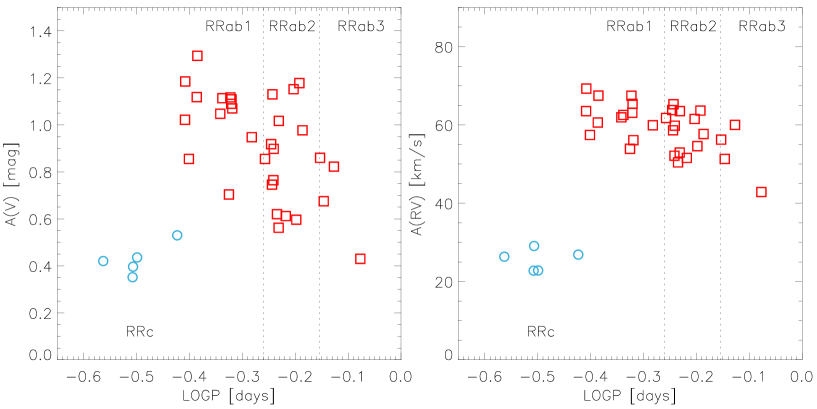
Figure 6: Left: Bailey diagram–optical amplitude versus logarithmic period–for TS RRLs. Red squares and blue open circles display RRab and RRc variables. The vertical dashed line separate the three period bins for RRab variables. Right: same as the left, but for iron $Amp(V)$.

We provide 28 RVC templates in total, by considering the combination of seven different spectroscopic diagnostics (H_α, H_β, H_γ, H_δ, Mg, Na, and Fe+Sr, see Table 4) and four period.

4.5 The reference epochs of the RVC templates

The photometric data available in the literature for the TS RRLs were not collected close in time with our spectroscopic data. Therefore, we cannot anchor the RVC templates to the photometric reference epochs (e.g., $T_{mean}^{opt}$). Small period variations and/or random phase shifts might significantly increase the dispersion of the points in the cumulative RVCs. The phase coverage of the TS RRLs is good enough to provide independent estimates of both the pulsation period and of the reference epoch. Moreover, $T_{mean}^{opt}$  matches $T_{mean}^{RV(Fe)}$  within 5% of the pulsation cycle (see Section 6 for more details), therefore we can adopt the latter to compute the RVC templates of the metallic lines (Fe, Mg, Na). This choice allows anyone to adopt $T_{mean}^{opt}$  to phase the RV measurements and then use our templates (see Appendix C for detailed instructions). Note that, to compute the RVC templates of the Balmer lines, we use $T_{mean}^{RV(H\beta)}$because there is a well defined difference in phase between $T_{mean}^{RV(H\beta)}$and $T_{mean}^{RV(Fe)}$. To provide a solid proof of our assumptions, we performed the same test discussed in Section 2.1.

We derived $T_{mean}^{RV}$  and $T_{min}^{RV}$from the average of the RVCs for both the Fe group lines and the H_β line, taken as representative of the Balmer lines. As expected, $T_{min}^{RV}$  matches in first approximation $T_{max}^{opt}$. Indeed, the latter was adopted by Liu (1991) and by Sesar (2012) to anchor their RVC templates. The working hypothesis behind this assumption is that the minimum in the RVC of the metallic lines takes place at the same phases at which the RVCs based on the Balmer lines attain their minimum, i.e. that $T_{min}^{RV(Fe)}$  matches $T_{min}^{RV(H\beta)}$. However, we checked this assumption and found that the mean difference in phase between the two epochs is 0.036$\pm$0.051, with the minimum in the radial velocity curves of Fe group lines leading the H_β minimum. Although the difference is consistent with being zero, its standard deviation is not negligible: a systematic phase drift of one twentieth around the minimum of the RVC might lead to offsets in the estimate of $V_{\gamma}$ of the order of 10 km/s.

We point out that TS RRLs have multiple estimates $V_{\gamma}$ and of $Amp(RV)$—three from the metallic lines plus four from individual Balmer lines—but they only have two reference epochs: one for the Fe group lines, representative of the metallic RVCs and one for H_β. The individual estimates of the reference epochs for the two groups of lines are listed in Table 6.

The basic idea is to have the different RVC templates phased at reference epochs originating from similar physical conditions. Weak metallic lines and strong Balmer lines display a well-defined RV gradient and their RVCs are also affected by a phase shift since the former form at high optical depths, and the latter at low optical depths (Liu & Janes 1990; Carney et al. 1992; Bono et al. 1994). We verified that the reference epochs for the weak metallic lines (Fe, Mg, Na) are the same within $\sim$3% of the pulsation cycle, while those for the Balmer lines, anchored to the H_β RVC, are the same within $\sim$5% of the pulsation cycle.

Figures 7 and 8 display the cumulative and normalized RVCs (CNRVCs) based on the Fe group lines and on the H_β line, respectively. Data plotted in these figures display two interesting features worth being discussed in detail. i)–The residuals between observations and analytical fits for the CNRVCs based on the Fe group lines and phased using the reference epoch anchored to $T_{mean}^{RV(Fe)}$  are systematically smaller than the residuals of the same CNRVCs anchored to $T_{min}^{RV(Fe)}$. The difference ranges from $\sim$30% for TS RRLs in the period bin RRab1 to $\sim$40% for TS RRLs in the period bin RRab3. ii)–The impact of the two different reference epochs is even more evident for the Balmer lines (Fig. 8). Indeed, the difference in the standard deviation ranges from $\sim$15% in the period bin RRc to $\sim$45% for the period bin RRab2. Moreover, the CNRVCs for the RRc and the RRab3 period bin show quite clearly that the reference epoch (vertical dotted line) anchored to $\tau_{0}$=$T_{mean}^{RV(Fe)}$  takes place at phases that are slightly earlier than the actual minimum (see right panels). This difficulty is associated with the shape of both light curves and RVCs and it causes larger and asymmetrical residuals when compared with the CNRVCs of the same period bin anchored to the mean magnitude/systemic velocity (see the histograms plotted in the panels to the right of the CNRVCs).

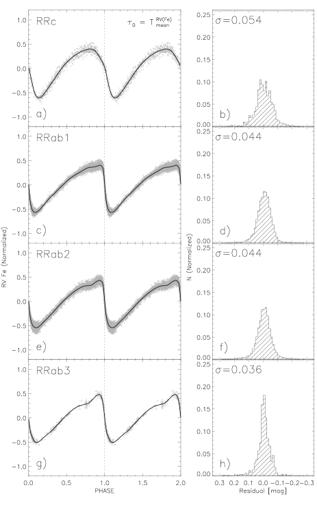
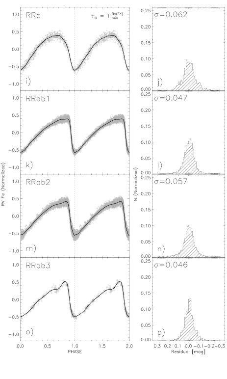
Figure 7: Same as Figure 2, but for the cumulative and normalized RVCs based on the Fe group lines. a), c), e) and g) panels versus i), k), m), and o) panels show the difference between RVCs phased by assuming as a reference epoch $\tau_{0}$=$T_{mean}^{RV(Fe)}$  and $\tau_{0}$=$T_{min}^{RV(Fe)}$, respectively. b), d), f), h), j), l), n) and p) panels display the residuals of the observations from the analytical fits.

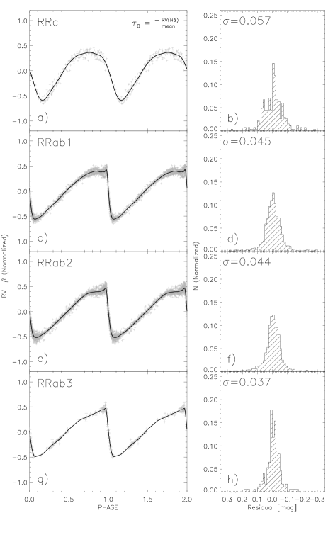
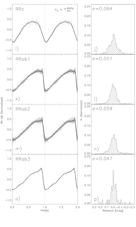
Figure 8: Same as Figure 7, but for cumulative and normalized RVCs based on the H_β line. Note that the a) to h) panels are anchored to $\tau_{0}$=$T_{mean}^{RV(H\beta)}$  and the i) to p) panels are anchored to $\tau_{0}$=$T_{min}^{RV(Fe)}$.

The current circumstantial evidence indicates that RVC templates based on Fe group RV measurements and anchored to $\tau_{0}$=$T_{mean}^{RV}$  provide $V_{\gamma}$ that are on average $\sim$30% more accurate than the same RVCs anchored to $\tau_{0}$=$T_{min}^{RV}$. The improvement in using $T_{mean}^{RV}$  compared with $T_{min}^{RV}$  becomes even more relevant in dealing with the RVCs based on Balmer lines. Indeed, uncertainties are smaller by up to a factor of three (see Section 7). This further supports the use of $T_{mean}^{RV}$  as the optimal reference epoch to construct RVC templates.

5 Radial velocity curve templates

Before deriving the RVC templates, two pending issues need to be addressed: are the RVCs for the different lines in the Fe group, in the Mg Ib triplet and in the Na doublet, within the errors, the same? Are the mean RVCs of these three groups of lines affected by possible systematics?

5.1 Mean RVC templates for the three different groups of metallic lines

Our dataset is large enough to derive RVC templates for each single absorption line listed in Table 4. However, our goal is to provide RVC templates that can be adopted as widely as possible. Therefore, we aim to provide one RVC template for each of the Balmer lines and one for each of the metallic groups (Fe, Na, Mg), making a total of seven different sets of RVC templates. This is feasible only if the RVCs of the lines belonging to the same group have, within the errors, the same intrinsic features, i.e. the same shape, amplitude and phasing.

In principle, the RVC derived with a specific absorption line is different with respect to the one derived from any another line, because different lines may form in different physical conditions of the moving atmosphere. This is quite obvious for the Balmer series, with $Amp(RV)$ progressively increasing by $\sim$60-70% from H_δ to H_α (S12, Bono et al. 2020a). This is the reason why independent RVC templates have to be provided for each Balmer line. However, for the Fe, Mg and Na groups, it is not a priori obvious whether different lines of the same group (e.g., Fe1 and Fe2) display, within the uncertainties, similar $Amp(RV)$ and RVC shapes. Therefore, we verified whether the RVCs within the Fe, Mg and Na groups agree within uncertainties.

To investigate on a quantitative basis the difference, we inspected the residuals of the RVCs of each line with respect to the average RVC of the group. The left panels in Fig. 9 display the residuals of the RV measurements based on Fe1, Fe2, Fe3 and Sr lines with respect to the average of the four lines. The middle and right panels are the same, but for the two Mg and the two Na lines. Note that we discarded all the Mg b1 RV measurements because this line is blended with an Fe I line (5167.50 $\;\buildrel\circ\over{\rm A}$). This iron line can be as strong as the Mg b1 line itself or even stronger depending on the Mg abundance and on the effective temperature. Therefore, even using high-resolution spectra the velocity measurements with the Mg b1 line refer to an absorption feature with a center that changes across the pulsation cycle.

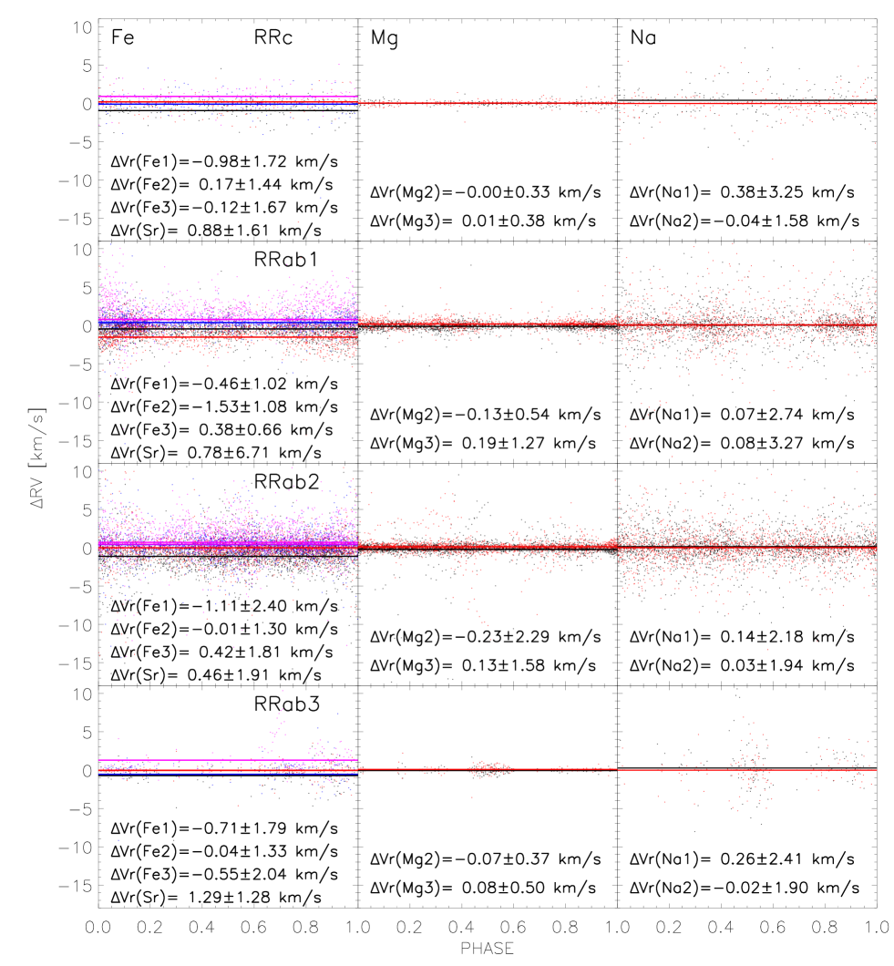
Figure 9: Left: Residuals of single-line Fe group RV measurements with respect to the mean RVC. Black (Fe1-mean), red (Fe2-mean), blue (Fe3-mean) and magenta (Sr-mean) symbols display the difference for the individual lines. The mean of the residuals are displayed as solid lines of the same color of the symbols and are labeled together with their standard deviations. From top to bottom, residuals are displayed for the four period bins. Middle: Same as the left, but for Mg RV measurements. Right: Same as the left, but for Na RV measurements.

Figure 9 displays, both quantitatively and qualitatively, that, for Mg and Na, there is no clear trend within the dispersion of the residuals. The maximum absolute offset is vanishingly small, being always smaller than 0.50 km/s, which is also smaller than our RV uncertainty. This means that these lines trace the dynamics of the same atmospheric layer and they can be averaged in order to derive a single set of RVC templates for both Mg and Na groups.

The same outcome does not apply to Fe and Sr lines. Indeed, although the average offsets are all smaller than the dispersions, they seem to follow a trend. More specifically, the average offset of the Fe1 curve is always smaller than the other, while the average offset of the Sr curve is typically larger. This is mostly due to the interplay of a small difference in $Amp(RV)$ (generally increasing from Fe1 to Sr) and a mild trend in the average velocity (generally increasing from Fe1 to Sr). However, all these offsets are smaller than the dispersions ($\leq$ 2.5 km/s) and similar to the intrinsic dispersion of the RVC templates (see Section 5.2). We also note that the standard deviation of the points around the offsets is, within the uncertainties, constant along the pulsation cycle. Indeed, a minimal increase around phase zero is only present for RV measurements based on iron in the period bin RRab1.

In the light of these results, we opted to derive three independent mean RVCs for the Fe, the Mg and the Na groups of lines. Selected RVCs for these three metallic diagnostics and for the four individual Balmer lines, anchored to $\tau_{0}$=$T_{min}^{RV(Fe)}$  and $\tau_{0}$=$T_{min}^{RV(H\beta)}$, are shown in Figures 10 and 11.

Figure 10: First row: From left to right radial velocity curves of the RRc variable CS Eri for the average Fe, Mg and Na groups of lines. Second row: Same as the top, but for the RRab1 variable HH Pup. Third row: Same as the top, but for the RRab2 variable RV Oct. Fourth row: Same as the top, but for the RRab3 variable AT Ser.

Figure 11: First row: From left to right radial velocity curves of the RRc variable CS Eri for individual Balmer lines (H_α, H_β, H_γ and H_δ). Second row: Same as the top, but for the RRab1 variable HH Pup. Third row: Same as the top, but for the RRab2 variable RV Oct. Fourth row: Same as the top, but for the RRab3 variable AT Ser.

5.2 Analytical fits of the RVC templates

To construct the RVC templates, we normalized the RVCs by subtracting $V_{\gamma}$ and dividing by $Amp(V_{r})$. Once normalized, we stacked the RVCs within the same period bin of RVC template, thus obtaining the CNRVCs (see Appendix B).

To provide robust RVC templates we decided to fit the CNRVCs with an analytical function. We discarded the Fourier series as a fitting curve because the number of phase points is not large enough (at least in the RRab3 period bin) to avoid non-physical bumps and spurious secondary features in the fits. We adopted the PEGASUS fit as for the light curve templates in Section 2.

Table 10: Coefficients and standard deviations of the PEGASUS fits to the CNRVCs.

Template	Bin	N	$A_{0}$	$A_{1}$	$\phi_{1}$	$\sigma_{1}$	$A_{2}$	$\phi_{2}$	$\sigma_{2}$	$A_{3}$	$\phi_{3}$	$\sigma_{3}$	$A_{4}$	$\phi_{4}$	$\sigma_{4}$	$A_{5}$	$\phi_{5}$	$\sigma_{5}$
				$A_{6}$	$\phi_{6}$	$\sigma_{6}$	$A_{7}$	$\phi_{7}$	$\sigma_{7}$	$A_{8}$	$\phi_{8}$	$\sigma_{8}$	$A_{9}$	$\phi_{9}$	$\sigma_{9}$				$\sigma$

Note. — We will provide this table only after the paper will be officially published on ApJ.

Table 10 provides the coefficients of the PEGASUS functions obtained from the fitting procedure. When possible, we favored the lowest possible order, especially for the RRc template, as first overtone pulsators have more sinusoidal RVCs. These are also the coefficients for the analytical form of the RVC templates. Figures 16 and  17 display the analytical fits of the RVC templates together with the observed RV measurements.

The largest standard deviations are those for the H_γ and H_δ RVC templates for the RRc period bin ($\sim$0.08 and 0.13, respectively). To convert the $\sigma$ into the uncertainty on $V_{\gamma}$, one has simply to factor in $Amp(RV)$. Since the typical $Amp(RV)$ for RRc variables in H_γ and H_δ range between 10 and 30 km/s (Bono et al. 2020b), the largest possible uncertainty introduced by the RVC template is of $\sim$4 km/s. However, the largest absolute uncertainties are associated with the H_α and H_β RVC templates for RRab1 period bin ($\sigma\sim$0.05). Since $Amp(RV)$ is much larger for these diagnostics, the absolute uncertainties on $V_{\gamma}$ based on these RVC templates are of $\sim$7 km/s. For metallic lines, all these uncertainties are on average smaller than $\sim$3 km/s. These results concerning both metallic and Balmer lines indicate that the current RVC templates can provide V_γ for typical Halo RRLs with an accuracy better than 1-3%.

6 Reference epoch to apply the radial velocity curve templates

A crucial aspect of templates is that they are used especially when the number of RV measurements is small. A first consequence is that, in a realistic scenario, the RV data is insufficient to accurately estimate $T_{mean}^{RV}$  for either metal or Balmer RVCs. However, optical photometry usually is conducted before spectroscopic observations, and a good knowledge of the pulsation period and of $Amp(V)$ are required to apply the RVC template. This means that we are typically dealing with a fairly well sampled $V$-band light curve, and in turn, with an accurate estimate of $T_{mean}^{opt}$. With this in mind, it is necessary to check whether $T_{mean}^{RV}$  and $T_{mean}^{opt}$  in RRLs take place, within the errors, at the same phase along the pulsation cycle. If this is the case, we could safely use of $T_{mean}^{opt}$  to phase the spectroscopic data and to apply the RVC template.

We phased a subset of RRLs with a good sampling of the pulsation cycle both in the $V$-band and in metallic RVCs. Fortunately, among the RRLs of the TS, there are several objects that were used for the Baade-Wesselink (BW) analysis and for which there are available $V$-band light curves and RVCs collected at relatively close epochs (at most within $\sim$3 years). This is an important advantage for this consistency test because possible changes in phases (phase drifts) and the effect of period derivatives are small. We derived both $T_{mean}^{RV(Fe)}$  and $T_{mean}^{opt}$  and they are listed in Table 11.

Table 11: Difference in the reference epoch between light and radial velocity curves. From left to right the columns give the ID, the pulsation mode, the pulsation period, $T_{mean}^{RV}$, $T_{mean}^{opt}$, the difference in phase and the reference.

Name	Type	Period	$T_{mean}^{RV(Fe)}$	$T_{mean}^{opt}$	$\Delta\Phi$	Ref.
		(days)	HJD-2,400,000 (days)
DH Peg	RRc	0.25551624	46667.5938	46684.6796	0.0239	0
TV Boo	RRc	0.31256	47220.7066	47227.5768	0.0260	1
T Sex	RRc	0.32468493	47129.6898	47226.4140	0.1229	1
RS Boo	RRab	0.37736549	46985.6766	46949.4482	0.0109	2
AV Peg	RRab	0.3903809	47130.3415	47123.3206	–0.0427	1
V0445 Oph	RRab	0.397026	45842.2860	46980.9462	–0.0111	3
RR Gem	RRab	0.3973	47220.6576	47226.5974	0.0498	1
TW Her	RRab	0.39959577	46925.8161	46947.3878	0.0168	2
AR Per	RRab	0.42556048	47128.3468	47123.6650	0.0019	1
V Ind	RRab	0.47959915	57619.5115	47814.0720	–0.0061	4
BB Pup	RRab	0.48055043	46136.1969	47192.9099	0.0052	5+6
TU UMa	RRab	0.5569	47129.8698	47227.4521	0.0088	1
SW Dra	RRab	0.56967009	46519.6350	46496.2706	0.0140	7
WY Ant	RRab	0.57434364	46135.3591	47193.2805	–0.0091	5+6
RX Eri	RRab	0.58725159	47130.7581	47226.4736	0.0096	1
RV Phe	RRab	0.59641862	47054.1546	46305.0578	–0.0075	8
TT Lyn	RRab	0.59744301	47129.6929	47123.1210	0.0003	1
UU Cet	RRab	0.60610163	47055.3286	47055.9229	0.0195	4
W Tuc	RRab	0.64224028	47057.8121	47493.2459	0.0046	4
X Ari	RRab	0.65117537	45640.8262	45639.5058	0.0278	9
SU Dra	RRab	0.66041178	47129.4805	47227.8778	0.0081	1
VY Ser	RRab	0.7141	44743.7769	47655.1533	–0.0120	3

Note. — In column 7, the references for the RVC and light curves adopted to derive $\Delta\Phi$ are listed in the following order:

Data listed in this table clearly show that $T_{mean}^{RV(Fe)}$  and $T_{mean}^{opt}$  trace, within the errors, the same phase along the pulsation cycle. Indeed the average phase difference is 0.007$\pm$0.019 and always smaller than 0.05 (see column 6 in Table 11) This means the two reference epochs provide the same phasing. As a consequence, the photometric $T_{mean}^{opt}$  can be safely adopted to anchor the RVC templates.

We already mentioned that there is a difference in phase between $T_{mean}^{RV(Fe)}$  and $T_{mean}^{RV(H\beta)}$. This means that, when adopting $T_{mean}^{opt}$  to use the template on Balmer lines, it is necessary to first shift the phases by an offset $\Delta\tau^{Fe}_{H\beta}$=$\Phi$($T_{mean}^{RV(Fe)}$-$T_{mean}^{RV(H\beta)}$). For this reason, we adopted the data listed in Table 6 and found a linear trend of $\Delta\tau^{Fe}_{H\beta}$ as a function of the pulsation period (see Fig. 12). The plausibility of the phase difference between metallic and Balmer lines is further supported by the empirical evidence that the standard deviation of the relation is vanishing (0.008). Indeed, it is almost one order of magnitude smaller than the standard deviation of the phase offset between $T_{min}^{RV(Fe)}$  and $T_{min}^{RV(H\beta)}$  (see Section 4.5).

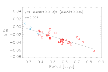
Figure 12: $\Delta\tau^{Fe}_{H\beta}$ versus period for the TS RRLs. The linear relation fitting the data is displayed as a solid line and labeled at the top, together with the standard deviation of the relation.

Large photometric surveys, however, often provide $T_{max}^{opt}$  but not $T_{mean}^{opt}$. To overcome this limitation and to facilitate the use of the RVC templates, we provide relations for $\Delta\Phi$ in Section 2.2 that allow the template user to easily convert the phases anchored on $\tau_{0}$=$T_{max}^{opt}$  can into phases anchored on $\tau_{0}$=$T_{mean}^{opt}$.

7 Validation of the radial velocity curve templates

A solid validation of the RVC templates requires that photometric and radial velocity measurements be as close as possible in time. This methodological approach provides the unique opportunity to derive accurate photometric (pulsation period, $V$-band mean magnitude, $Amp(V)$, reference epoch) and spectroscopic ($V_{\gamma}$) properties of the RRLs adopted for the validation. We have already mentioned in Section 4.5 that the temporal proximity of both photometric and spectroscopic data is only available for a small number of field RRLs. To overcome this limitation we decided to select from the calibrating sample one RRL per period bin: YZ Cap for the RRc, V Ind for the RRab1, W Crt for the RRab2 and AT Ser for the RRab3. We label these four RRLs as the Template Validation Sample (TVS) and they are the benchmark for the RVC template validation.

Ideally, the validation should be done with an RRL sample independent from the one adopted to construct the RVC templates. However, we have verified that, by removing the four TVS RRLs from the calibrating RRLs, the coefficients of the analytical fits are only minimally affected. Note that the selection of the validating variable might bias the uncertainties of the result because there is a small degree of internal variation in the shape of the RVCs of the different period bins. To investigate on a quantitative basis the dependence on the validating variable, we performed several tests by using as validating variable one after the other all the RRLs included in each period bin. Interestingly enough, we found that the medians (see Tables 12 and 13) agree within 1$\sigma$, while the variation of the dispersions is on average smaller than 20%. This means that the selection of the validating variable has a minimal impact on the accuracy of the validation.

We adopted the $V_{\gamma}$ of the TVS RRLs obtained by directly fitting their RVCs (see Tables 8 and  9) and assumed these as the best estimates for the systemic velocity ($V_{\gamma(best)}$) to be used in the validation process. However, to use the RVC template we need to convert $Amp(V)$ into $Amp(RV)$ and then use the latter to rescale the normalized analytical function. The ratio between $Amp(V)$ and $Amp(RV)$ together with the equations for the conversion are thoroughly discussed in Appendix A.

The analytical form of the RVC templates can be used both as curves to be anchored to a single phase point and as functions to fit a small number of phase points (three or more). Therefore, we followed two different paths for the validation process, based either on a single phase point approach (Section 7.1) or on multiple phase points (Section 7.2). The key idea is to estimate the accuracy of the light-curve templates from the difference $\Delta V_{\gamma}$ between $V_{\gamma(best)}$ and the systemic velocities estimated by adopting the RVC template ($V_{\gamma(templ)}$). Furthermore, the accuracy of the current RVC templates is quantitatively compared, using TVS RRLs, with similar RVC templates available in the literature (S12).

7.1 Single phase point

As a first step, we generated a grid of 100 phase points for the seven RVCs (Fe, Mg, Na, H_α, H_β, H_γ, H_δ, that we label, respectively, with a $j$ index running from 1 to 7). We interpolated the analytical fits of the RVCs for the TVS RRLs on an evenly-spaced grid of phases ($\phi_{i}$=[0.00, 0.01, … 0.99], where $i$ runs from 1 to 100). For each $\phi_{i}$ and each RVC($j$), we generated a RV measurement with the sum $RV_{ij}=RV(fit(\phi_{i}))_{j}+r\sigma$. The two addenda are: i) $RV(fit(\phi_{i}))_{j}$, which is the value of the fit of the RVC($j$) interpolated at the phase $\phi_{i}$; ii) $r\sigma$, which simulates random noise: $\sigma$ is the standard deviation of the phase points around the fit and $r$ is a random number extracted from a standard normal distribution.

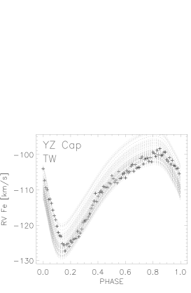
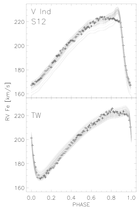
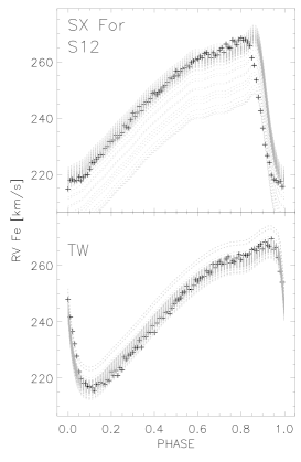
Figure 13: Left: Black crosses show the Fe RV measurements that we generated from the grid for the RRc variable YZ Cap. Gray dashed lines display the RVC templates from this work (labeled as TW) associated with each phase point. The ID of the RRL is labeled. Note that the comparison with the RVC template provided by S12 is missing because YZ Cap is an RRc variable. Middle: Same as the left, but for the RRab variable V Ind belonging to the RRab1 period bin. Top: Radial velocity curves based on the RVC templates provided by S12. Bottom: same as the top, but based on our RVC templates. Right: Same as the middle, but for the RRab variable SX For belonging to the RRab2 period bin.

We applied the RVC templates on each of the simulated points, thus deriving 100 estimates of the systemic velocity ($V_{\gamma(i,j)}^{templ}$) for each RVC($j$). To provide a quantitative comparison, these estimates were performed using both our own and S12 RVC templates. The S12 RVC templates were not applied to YZ Cap, since they are valid only for RRab variables. In discussing the difference between our own RVC templates and those provided by S12, there are three key points worth being mentioned: i)– the comparison for Fe, Mg and Na RVCs was performed by using the generic metallic RVC template from S12, because they do not provide specific-element RVC templates; ii)– the RVC templates by S12 were anchored to $T_{max}^{opt}$, while our own were anchored to $T_{mean}^{opt}$; iii)– the RVC templates by S12 were rescaled, for internal consistency, by using their conversion equations from $Amp(V)$ to $Amp(RV)$ and not our own equation for the amplitude ratio.

Note that, due to the paucity of RRab3 variables, it was not possible to find one with both a reliable estimate of the reference epoch and with RV measurements close in epoch to the optical light curve. Therefore, the RVC templates for the RRab3 period bin were not validated with the single phase point approach. Nonetheless, we anticipate that we successfully validated the RRab3 RVC templates with the three-point approach (see section 7.2). Figure 13, displays the simulated RV(Fe) phase points and the RVC templates applied to them. Finally, we derived the offsets $\Delta V_{\gamma(i,j)}=V_{\gamma(i,j)}^{templ}-V_{\gamma(j)}^{best}$ for each point and each RVC template. Table 12 gives the median and standard deviations of $\Delta V_{\gamma}$ for each RVC template.

Table 12: Validation of the RVC templates based on the single phase point approach.

	$\Delta V_{\gamma}$(Fe)		$\Delta V_{\gamma}$(Mg)		$\Delta V_{\gamma}$(Na)		$\Delta V_{\gamma}$(Hα)		$\Delta V_{\gamma}$(Hβ)		$\Delta V_{\gamma}$(Hγ)		$\Delta V_{\gamma}$(Hδ)
Name	mdn	$\sigma$	mdn	$\sigma$	mdn	$\sigma$	mdn	$\sigma$	mdn	$\sigma$	mdn	$\sigma$	mdn	$\sigma$
	(km/s)		(km/s)		(km/s)		(km/s)		(km/s)		(km/s)		(km/s)
—Our RVC templates—
YZ Cap	–0.082	2.270	–0.548	2.755	–0.970	2.600	–0.815	3.027	–1.116	3.131	0.202	2.566	0.062	2.906
V Ind	–0.301	1.925	–0.173	2.271	0.469	1.729	–0.940	2.847	0.055	2.998	0.203	2.357	–0.194	2.505
SX For	0.066	2.138	–0.257	2.670	–0.241	1.887	1.063	3.181	0.527	3.110	0.725	4.293	1.007	3.347
—S12—
V Ind	0.049	2.977	–0.583	3.287	0.440	3.200	0.685	4.356	0.877	6.601	0.644	6.895	…	…
SX For	1.488	5.418	1.115	5.583	1.467	5.634	3.863	8.812	3.820	10.926	4.154	10.899	…	…

Note. — Medians (mdn) and standard deviations ($\sigma$) of for the $\Delta V_{\gamma}$ based on a single phase point validation, for both our and S12 RVC templates.

We note that that the median of the $\Delta$V is always smaller, in absolute value, than 1.0 km/s and 1.5 km/s for metallic and Balmer RVC templates. In all cases, the standard deviations are larger than the residuals, meaning that the latter can be considered vanishing within the dispersion. The largest standard deviations are found for the H_α and H_β RVC templates and progressively decrease when moving to H_γ, H_δ and metallic lines.

The comparison between the current and the RVC templates provided by S12 brings forward that the standard deviations of the former ones are systematically smaller by a factor ranging from $\sim$1.5 to $\sim$3. The higher accuracy of the current RVC templates is due to an interplay of a more robust estimate of T_mean with respect to T_max and a more accurate optical-to-RV amplitude conversion (note e.g., in the upper-right panel of Fig. 13, $Amp(RV)$ is clearly overestimated for the S12 RVC template).

7.2 Multiple phase points

To apply the RVC templates to single phase points, it is necessary to know four parameters with great accuracy: i) the pulsation period, ii) the pulsation mode, iii) $Amp(V)$ and iv) the reference epoch of the anchor point ($T_{mean}^{opt}$). The last one is particularly delicate, not only because a good sampling of the light curve is needed but also because, when the spectroscopic data were collected several years before/after the photometric data, even small phase shifts or period changes can affect the phasing of the RV measurements. Note that for RRLs affected by large Blazhko modulations, these parameters—especially $Amp(V)$ and reference epoch—cannot be accurately estimated. Therefore we suggest to avoid the application of the templates to RRLs with evident Blazhko modulations.

To overcome this limitation, it is possible to use the RVC templates as fitting functions if at least three RV measurements are available. In this empirical framework, only three parameters are required in order to apply the RVC template, namely the pulsation period, the pulsation mode and $Amp(V)$. We performed a number of tests by assuming that three independent RV measurements were available. In this approach, the $Amp(V)$ has to be converted into the $Amp(RV)$ and then perform a least-squares fit of the RV measurements by adopting the RVC template as the fitting function. The minimization of the $\chi^{2}$ is based on two parameters: $\Delta\phi$ (a horizontal shift) and $\Delta V_{\gamma}$ (a vertical shift). The function to be minimized is:

$$P(\phi;\Delta\phi,\Delta V_{\gamma})=\Delta V_{\gamma}+Amp(RV)\cdot\Big{(}A_{0}^{P}+\Sigma_{i}A_{i}^{P}\exp{\Big{(}-\sin{\Big{(}\dfrac{\pi(\phi-\phi_{i}-\Delta\phi)}{\sigma_{i}^{P}}\Big{)}^{2}}\Big{)}\Big{)}}$$ (2)

To simulate three RV measurements, we extracted three random phases over the pulsation cycle and generated three RV measurements following the same approach adopted in Section 7.1. To rely on a wide statistical sample, the process was repeated 5000 times to generate 5000 different triplets of RV measurements for each RVC template. Henceforth, we label each of the triplets with a subscript $k$.

We estimated the systemic velocity $V_{\gamma(k,j)}^{templ}$ by fitting each of the triplets with both S12 and our own analytical form of the RVC templates. Analogously to Section 7.1, we derived the offsets $\Delta V_{\gamma(k,j)}$ and their median and standard deviations and they are listed in Table 13.

We note that the uncertainties are larger for the three-point approach with respect to the single point one discussed in the former section. This happens because, when the three points are randomly extracted, it may happen that two (or all) of them are too close in phase, and the fitting procedure provides less solid estimates. This is a realistic case in which one might not have control over the sampling of the spectroscopic data. Also, the very fact that we are fitting the shift in phase, and not anchoring the RV data to the true reference epoch of the variable, means that the phasing of the template is not fixed, and this naturally leads to larger uncertainties. We have verified that, if the reference epochs were available, we would obtain standard deviations that are $\sim$10-30% smaller and medians that are up to $\sim$50% smaller than in the case of the single-epoch approach.

Table 13: Results of the validation for the multiple phase point approach.

	$\Delta V_{\gamma}$(Fe)		$\Delta V_{\gamma}$(Mg)		$\Delta V_{\gamma}$(Na)		$\Delta V_{\gamma}$(Hα)		$\Delta V_{\gamma}$(Hβ)		$\Delta V_{\gamma}$(Hγ)		$\Delta V_{\gamma}$(Hδ)
Name	mdn	$\sigma$	mdn	$\sigma$	mdn	$\sigma$	mdn	$\sigma$	mdn	$\sigma$	mdn	$\sigma$	mdn	$\sigma$
	(km/s)		(km/s)		(km/s)		(km/s)		(km/s)		(km/s)		(km/s)
—Our RVC templates—
YZ Cap	0.028	3.049	1.682	2.857	0.873	3.666	4.147	5.813	0.742	3.863	–1.702	5.413	4.839	4.799
V Ind	–0.472	5.658	0.808	4.649	–0.621	6.230	6.268	17.383	3.227	11.646	2.620	9.894	2.978	8.356
SX For	1.436	8.031	2.943	8.068	1.840	9.490	4.373	16.630	1.700	12.225	3.050	10.995	4.196	9.721
AT Ser	0.219	9.340	2.311	11.129	0.363	12.087	–0.583	17.990	–0.844	15.311	–0.371	13.432	4.477	12.727
—S12—
V Ind	–0.273	7.822	0.770	9.314	-0.777	9.805	4.817	19.250	2.676	13.259	2.263	12.345	…	…
SX For	2.297	7.673	3.953	7.502	2.437	9.102	3.988	16.418	2.207	11.638	3.522	10.763	…	…
AT Ser	0.454	9.522	2.412	10.869	0.528	11.037	1.251	19.826	0.989	16.109	1.289	13.684	…	…

Note. — Medians (mdn) and standard deviations ($\sigma$) for the $\Delta V_{\gamma}$ obtained from the three-points validation, for both our and S12 RVC templates.

Note that we did not put any restriction on which RV measurements were chosen to form a triplet. More specifically, we did not remove triplets in which two phase points were very close in phase, thus mimicking a realistic situation where either only two RV independent measurements were obtained or where the points are really close in phase due to the sampling of the spectroscopic data. Although this scenario usually leads to flawed estimates of $V_{\gamma}$, they are a minority, with less than $\sim$10% of the triplets having points closer than 0.05 in phase. Moreover, it is not only the difference in phase that matters but also the distribution along the pulsation cycle. Indeed, phase points close in phase located along the decreasing branch of RRab variables produce larger uncertainties when compared with other phase intervals. The decision to keep even these troublesome triplets in our tests allowed the computed errors to take into account all the possible drawbacks of real observations, including the scenario of spectroscopic surveys that scan the sky by taking multiple consecutive measurements.

Data listed in Table 13 show that, with the only exception of the RRab3, for which the standard deviations are similar, our RVC templates provide smaller standard deviations of the $\Delta$V compared to S12 templates. This is true even for the three phase points validation, where the median offsets are smaller than the standard deviations. This means that the RVC template provides $V_{\gamma}$ estimates that are more accurate than the simple average of the three RV measurements.

8 RR Lyrae in NGC 3201 as a test case

The Galactic globular cluster (GGC) NGC 3201 is a nearby (4.7 kpc, Vasiliev & Baumgardt 2021) metal intermediate ([Fe/H]$\sim$ –1.4 Mucciarelli et al. 2014; Magurno et al. 2018) stellar system hosting a sizeable number of RRLs (77 RRab, 8 RRc, 1 candidate RRd, Piersimoni et al. 2002; Layden & Sarajedini 2003; Arellano Ferro et al. 2014) This cluster has a very high RV: 494.5$\pm$0.4 km/s based on giant and subgiant stars and 496.47$\pm$0.11 km/s based on turn-off, subgiant and red giant stars (Ferraro et al. 2018; Wan et al. 2021, respectively). Note that Magurno et al. (2018) adopted the S12 RVC templates and applied them to eleven RRLs in NGC 3201 obtaining a cluster RV of 494$\pm$2$\pm$8 km/s which is within 1$\sigma$ of literature estimates. Interestingly, by taking advantage of accurate proper motion measurements based on Gaia DR2 Massari et al. (2019) suggested that NGC 3201 is likely an object accreted during either the Sequoia or the Gaia-Enceladus merger.

To investigate on a more quantitative basis the cluster properties, we used the MUSE@VLT spectra collected by Giesers et al. (2019) for seven cluster RRab variables. From these spectra, we measured H_α and H_β RVs (see data listed in Table 15) and the RVCs are displayed in Figure 14.

Table 14: Properties of the RRLs observed by MUSE in NGC 3201

Name	Type	Period	$V$	$Amp(V)$	$T_{mean}^{opt}$	$T_{max}^{opt}$	$V_{\gamma}$(Hα)	$V_{\gamma}$(Hβ)
		(days)	(mag)		HJD-2,400,000 (days)		(km/s)
V5	RRab	0.501527	14.786	…	…	…	497.9$\pm$3.5	500.1$\pm$2.8
V17	RRab	0.565590	14.794	0.824	56374.33072	56373.80043	501.0$\pm$3.3	501.6$\pm$3.0
V23	RRab	0.586775	14.795	0.742	56374.44344	56374.50391	496.4$\pm$3.8	493.1$\pm$3.0
V50	RRab	0.542178	14.795	0.876	56374.15802	56374.19955	499.0$\pm$3.2	498.6$\pm$3.4
V77	RRab	0.567644	14.672	0.829	56374.05485	56374.10073	483.2$\pm$3.3	488.0$\pm$3.2
V90	RRab	0.606105	14.706	1.048	56374.21846	56374.27385	489.8$\pm$3.1	493.0$\pm$3.0
V100	RRab	0.548920	14.786	0.863	…	…	495.6$\pm$3.2	496.1$\pm$3.1

Table 15: Radial velocity measurements for RRLs in NGC 3201.

Name	Species	HJD	RV	eRV
		(days)	(km/s)
V5	Halpha	2456978.8484	487.562	4.023
V5	Halpha	2456989.8680	513.958	3.719
V5	Halpha	2457008.8324	547.947	4.861
V5	Halpha	2457009.8025	530.079	2.620
V5	Halpha	2457131.4746	472.353	3.208
V5	Halpha	2457134.4825	470.448	2.996
V5	Halpha	2457138.4761	473.754	3.604
V5	Halpha	2457419.7608	462.131	3.225
V5	Halpha	2457421.7614	458.032	4.901
V5	Halpha	2457787.8737	456.275	3.388

Note. — Only ten lines are listed. The machine-readable version of this table is available online on the CDS.

Unfortunately, the optical light curves that we adopted from Arellano Ferro et al. (2014) do not fully cover the pulsation for all the cluster RRLs. More specifically, we could not derive a reliable estimate of the reference epochs for V5 and V100. Due to this, we are not able to apply the templates to these two stars. In principle, we could apply the three-point method, but we wanted to keep our V_γ estimates as homogeneous as possible.

After deriving—with the PLOESS algorithm—the best estimate for the systemic velocity ($V_{\gamma(best)}$, displayed in Table 14) by fitting the RVCs, we applied the RVC template by using the single phase point approach. Note that, in this case, we do not generate a grid of synthetic points, but we simply extract the points one by one from the RVC. Table 16 shows the average $V_{\gamma(templ)}$ estimates for all the lines, together with the standard deviation and the median of the offsets. The results are similar to those found in Section 7.1, meaning that all the medians are smaller than the standard deviations and, on average, the standard deviations obtained by using our own RVC templates are smaller than those coming from the use of the S12 RVC templates.

Our final estimate for the velocity of the whole system, by using both H_α and H_β is 496.89$\pm$8.37 (error) $\pm$3.43 (standard deviation) km/s by using the RVC templates and 495.21$\pm$3.23 (error) $\pm$4.32 (standard deviation) km/s by simply fitting the RVCs, which agree quite well, within 1$\sigma$, with similar estimates available in the literature.

Table 16: Systemic velocities of the RRLs in NGC 3201 based on the RVC templates.

	Hα			Hβ
Name	$V_{\gamma(templ)}$	$\sigma V_{\gamma(templ)}$	mdn$\Delta$V	$V_{\gamma(templ)}$	$\sigma V_{\gamma(templ)}$	mdn$\Delta$V
	(km/s)			(km/s)
	—Our RVC templates—
V17	500.4	6.0	–0.6	499.4	5.6	–2.3
V23	495.7	6.1	–0.6	498.1	8.8	4.9
V50	498.0	6.3	–1.0	498.0	5.5	–0.6
V77	486.9	12.2	3.6	489.4	8.0	1.4
V90	491.1	10.3	1.3	494.8	10.7	1.8
	—S12—
V17	496.2	15.3	–4.8	498.5	9.4	–3.2
V23	498.6	9.2	2.2	497.5	10.2	4.3
V50	499.3	5.3	0.3	497.1	7.3	–1.5
V77	488.3	12.1	5.1	488.3	11.7	0.3
V90	492.3	18.3	2.5	494.1	22.3	1.1

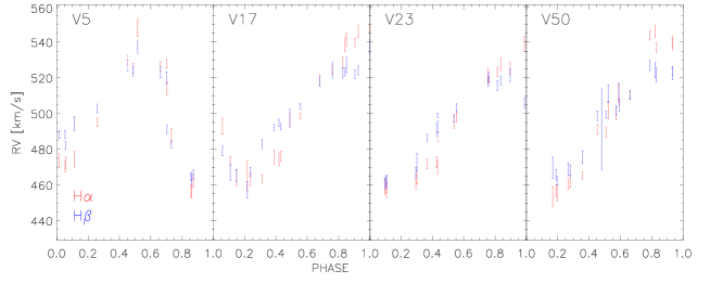
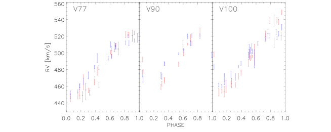
Figure 14: Red: H_α RV measurements; Blue: H_β RV measurements. The phases in the figures were derived by adopting the period and the reference epoch ($T_{mean}^{opt}$) displayed in Table 14. For V5 and V100, we have assumed an arbitrary reference epoch, since we could not derive an accurate estimate from the optical light curves.

9 Summary and final remarks

We provide accurate and homogeneous RVC templates for both RRab and RRc variables using for the first time spectroscopic diagnostics based on well-identified metallic (Fe, Mg, Na) lines and on Balmer (H_α, H_β, H_γ, H_δ) lines. In the following we discuss the approach adopted to construct the RVC templates and summarize the most relevant results.

$V$-band light curve templates — To demonstrate on a quantitative basis the difference between the reference epoch anchored to the maximum brightness and to the mean magnitude along the rising branch, we collected homogeneous $V$-band photometry for cluster ($\omega$ Cen , M4) and field RRLs. We have grouped them into four period bins (the same that we have used for the RVC templates) and found that the anchoring to the epoch of the mean magnitude on the rising branch ($T_{mean}^{opt}$) provides smaller standard deviations on the light curve templates than the anchoring to the maximum brightness ($T_{max}^{opt}$). The decrease is of the order of 35% for the period bins with cuspy light curves (RRab1, RRab2) and of 45% for those with flat-toopped light curves. These finding strongly supports the results obtained by Inno et al. (2015) and by Braga et al. (2019) in using $T_{mean}^{opt}$  to phase the NIR light curves of both classical Cepheids and RRLs.

Spectroscopic catalog — In this work, we present the largest collection of RRL spectra ever compiled in the literature. Altogether, we collected 23,865 spectra for 7,070 RRab and 3,343 RRc variables. These measurements were secured using eleven different spectrographs, ranging from low (2,000) to very high spectral resolution (115,000). To build the RVC templates, the most important dataset is the du Pont (see Table 3). Spectroscopic observations at this telescope were specifically planned to cover the entire pulsation cycle of several bright RRLs ($<V>\sim$10-11 mag for the majority of them). We also collected RV measurements and $V$-band time series from the literature (the Baade-Wesselink [BW] sample), which were crucial to investigate the reference epoch and the ratio between RV and optical amplitudes.

Amplitude ratio — To apply the RVC templates, it is necessary to have prior knowledge on the optical amplitude of the variable, to correctly rescale the RVC template itself and to optimally match the true RVC. We provide new equations for the ratio of $Amp(RV)$ over $Amp(V)$. Those available in the literature (S12), for RVCs based on metallic and Balmer (H_α, H_β, H_γ) lines, were constructed using six RRab variables covering a very narrow range in pulsation period (0.56-0.59 days). In this investigation we provide different RVC templates for both RRc and RRab variables based on metallic and Balmer (H_α, H_β, H_γ, H_δ) lines. Even more importantly, our relations are based on three dozen variables covering a wide range in pulsation periods (0.27-0.83 days) and metal content (–2.6$\lesssim$[Fe/H]$\lesssim$0.0).

Reference epoch — When applying the RVC template to single RV measurements, it is necessary to anchor the RVC template at the same epoch of the observations. The RVC templates are applied to RRLs with well sampled optical light curves and a few spectroscopic measurements. Therefore, the only pragmatical possibility to phase the spectroscopic data is to derive a reference epoch from the light curve. By using the light curves and the RV curves of our BW sample, we demonstrated that $T_{mean}^{opt}$  is, within 5% of the pulsation cycle, identical to the time of mean velocity on the decreasing branch of the Fe RVC ($T_{mean}^{RV(Fe)}$). This means that RVC templates based on Fe, Mg and Na lines can be safely anchored to $T_{mean}^{RV(Fe)}$, and this approach does not introduce any systematic error when $T_{mean}^{opt}$  is adopted to apply the RVC template. We also found that RVCs based on Balmer lines display a well defined phase lag across the phases of mean RV. Therefore, we decided to anchor the current H_α, H_β, H_γ and H_δ RVC templates to the time of mean velocity on the decreasing branch of the H_β RVC ($T_{mean}^{RV(H\beta)}$), taken as representative of the Balmer lines. Additionally, we found a clear trend in the phase difference between $T_{mean}^{RV(Fe)}$  and $T_{mean}^{RV(H\beta)}$  as a function of the pulsation period. The new analytical relation gives the phase difference required to use the Balmer RVC templates, because $T_{mean}^{opt}$  does not match $T_{mean}^{RV(H\beta)}$.

To discuss the concerning pros and cons of the reference epochs anchored to $T_{mean}^{RV}$  and to $T_{min}^{RV}$  into a more quantitative framework, we performed a series of numerical experiments. Interestingly enough, we found that RVC templates based on metallic RV measurements and anchored to $\tau_{0}$=$T_{mean}^{RV}$  provide $V_{\gamma}$ that are on average $\sim$30% more accurate than the same RVCs anchored to $\tau_{0}$=$T_{min}^{RV}$. Even more importantly, we found that the improvement in using $T_{mean}^{RV}$  compared with $T_{min}^{RV}$  becomes even more relevant in dealing with RVCs based on Balmer lines. Indeed, the uncertainties decrease up to a factor of three (see Section 7). The current circumstantial evidence further supports not only the use of two independent reference epochs for metallic and Balmer lines, but also the use of $T_{mean}^{RV}$  as the optimal reference epoch to construct RVC templates.

Finally, we investigated the correlation in phase between $T_{mean}^{opt}$  ($\Phi_{mean}$) and $T_{max}^{opt}$  ($\Phi_{max}$). This search was motivated by the fact that the current photometric surveys only provide reference epochs anchored to the time of maximum light ($T_{max}^{opt}$). We found that the difference between the two ($\Delta\Phi_{max-min}=\Phi_{max}-\Phi_{min}$) is constant—within the dispersion—for RRc variables and it follows a linear trend for RRab variables. We provide these relations for those interested in using the current RVC templates to RRLs for which only $T_{max}^{opt}$  reference epochs are available.

Radial velocity curve templates — We provide a total of 28 RVC templates of RRLs: these are divided into four different period bins (one for the RRc and three for the RRab variables) and seven diagnostics (Fe, Mg, Na, H_α, H_β, H_γ and H_δ). The analytical form of the templates is provided in the form of a PEGASUS series (fifth to ninth order). Analytical fits based on PEGASUS series, when compared with Fourier series, do not display spurious ripples when there are neither gaps in the phase coverage nor in the case of uneven sampling. The RVC templates have intrinsic dispersions that lead to errors smaller than 10 km/s in the worst case (H_α and H_β for high amplitude RRLs) and one order of magnitude smaller for the RVC templates with the smaller intrinsic dispersion (metallic lines RVC templates). To maximize the reach of the results of this work, we provide, in Appendix C, clear instructions on how to apply the RVC templates in different real-life observational scenarios.

Template validation — To validate the current RVC templates we performed a detailed comparison with the RVC templates provided by S12 for RRab variables and based on metallic and Balmer (H_α, H_β, H_γ) RVCs. We performed these tests on a sub-sample of variables that were used to build the RVC template (YZ Cap, V Ind, W Tuc, AT Ser). The validation process was performed using both a single phase point approach, where the knowledge of the reference epoch is mandatory, and with a three phase points approach, where the RVC template is used as a fitting function. We found that the median offset of the $V_{\gamma}$ estimates from the RVC templates is always smaller than 1.5 km/s (one point approach) and 6 km/s (three point approach). The medians are smaller than the standard deviations, meaning that systematic errors are negligible with respect to the statistical errors. We also found that our RVC templates provide $V_{\gamma}$ estimates that have a dispersion smaller by a factor of 1.5-3 than those based on the RVC templates provided by S12.

RRLs in NGC 3201 — We reduced the MUSE spectra already presented in Giesers et al. (2019) and obtained H_α and H_β RVCs. We derived V_γ both by fitting the RVC and by extracting the measurements one by one, and by adopting the RVC templates. Their results based on these RV measurements are very similar to those of the validation process, with offsets smaller than 6 km/s and standard deviations that are smaller than those on the S12 RVC templates. Our estimate of the $V_{\gamma}$ of the cluster is 496.9$\pm$8.4 (error) $\pm$3.4 (standard deviation) km/s from the RVC templates and 495.2$\pm$3.2 (error) $\pm$4.3 (standard deviation) km/s from the fit with the RVC templates. They both agree, within 1$\sigma$, with literature estimates.

In the next coming years the ongoing (OGLE, ASAS-SN, ZTF, sky-mapper, PanSTARRS) and near future (VRO) ground-based and space-based (Gaia, WISE, WFIRST) observing facilities will provide a complete census of evolved variable stars associated with old stellar tracers in the Milky Way and in Local Group galaxies. This will open new paths in the analysis of the early formation and evolution of the Galactic spheroid. However, firm constraints on the formation mechanism, namely, the dissipative collapse (Eggen 1962), dissipation-less mechanism (Searle & Zinn 1978) and Cold Dark Matter cosmological models (Monachesi et al. 2019) require detailed information concerning the kinematics and the metallicity distribution of the adopted stellar tracers. This is the approach already adopted to fully characterize the stellar streams and the merging history of the Galactic Halo (Helmi et al. 2018; Vasiliev 2019; Prudil et al. 2021).

Upcoming and ongoing low- (LAMOST-LR, Su et al. 1998; SDSS Aguado et al. 2019), medium- (4MOST, de Jong et al. 2012; SEGUE, Yanny et al. 2009; GALAH, Buder et al. 2018; HERBS, Duong et al. 2019; LAMOST-MR, Su et al. 1998; RAVE, Steinmetz et al. 2006; WEAVE, Dalton et al. 2012) and high-resolution (APOGEE, Majewski et al. 2017; MOONS, Taylor et al. 2018; PFS, Tamura et al. 2018) spectroscopic surveys will provide a wealth of new data for large samples of dwarf and giant field stars. In this context, old variable stars play a crucial role because their individual distances can be estimated with a precision of the order of 3-5% within the Local Group. Recent spectroscopic investigations based on high resolution spectroscopy (For et al. 2011; Sneden et al. 2017; Crestani et al. 2021a) indicate that detailed abundance analysis can be performed with spectra collected at random phases. Unfortunately, the typical limiting magnitudes for spectroscopic investigations are roughly five magnitudes brighter than photometric ones, with current spectrographs available at the 8-10m class telescope allowing us to reach limiting magnitudes of the order of V$\sim$20-21 mag. However, even with the usage of large telescopes, the estimate of V_γ is time consuming, because it requires a spectroscopic time series of at least a dozen points. The RVC templates developed in this investigation provide new solid diagnostics to provide accurate V_γ determinations by using a small number (three or less) of RV measurements, based on low-resolution spectra. Highly accurate estimates of line-of-sight velocities of stream stars are imperative for constraining the dark matter distribution (Bonaca & Hogg 2018); these RVC templates will provide just that for the numerous RRL harbored by MW streams. The current diagnostics are focused on spectroscopic features located either in the blue or in the visual wavelength regime. A further extension into the red and the near-infrared regime is mandatory to fully exploit the most advanced space (Gaia, Gaia Collaboration et al. 2016; JWST, Gardner et al. 2006; Roman Spergel et al. 2015) and ground-based (GMT, ELT, TMT) observing facilities.

Appendix A Amplitude ratios

The fundamental piece of information that is needed to use the RVC template RVCs is the relation of $Amp(RV)$ vs $Amp(V)$. These relations should be adopted to re-scale the normalized templates to the true $Amp(RV)$ of the star, with the knowledge of $Amp(V)$. The leading argument is always that, since there is far more availability of light curves than of RVCs, the amplitudes of the former should be adopted to derive those of the latter.

For their RVC templates, S12 adopted $Amp(RV)$ vs $Amp(V)$ relations based on six RRLs for metallic lines, H_α, H_β and H_γ. We provide the same relations, but separating RRc and RRab variables. We have considered the use of $Amp(RV)$ vs $Amp([3.6])$ relations, since the [3.6] band traces radius variations and is not affected by temperature variations as the $V$ band. However, there are two arguments against this option: $i)$— there is paucity of MIR light curves respect to optical light curves; $ii)$— There is mounting empirical evidence that amplitude ratios using NIR and MIR bands follow a mild trend with metallicity (Mullen et al. 2021).

Before deriving the relation between $Amp(RV)$ and $Amp(V)$, we checked whether we could assume the Fe, Mg and Na amplitudes as equivalent. Figure 15 shows the residuals of Na and Mg $Amp(RV)$ versus the Fe $Amp(RV)$. It is clear that there is no trend with period and also the offset is well within the $Amp(RV)$ uncertainty. This means that we can provide only two $Amp(RV)$ vs $Amp(V)$ relations (one for RRc and one for RRab variables) that hold for both Fe, Mg and Na. We also collected RV curves of RRLs from literature, all derived from metallic lines (BW sample, see caption of Table 11). We found that the BW $Amp(RV)$ displays a very small difference with our Fe $Amp(RV)$ (0.23$\pm$3.73 km/s). This allowed us to merge the two sets of $Amp(RV)$ and derive a more solid relation for the metallic $Amp(RV)$, based on a larger number of objects (12 RRc and 60 RRab).

The right panels of Figure 15 display the trend of Fe and of the Balmer $Amp(RV)$ with $Amp(V)$. A steady increase of the slopes for the Balmer $Amp(RV)$, from $\delta$ to $\alpha$ is clear enough, both visually in the figure and quantitatively from the coefficients listed in Table 17. This is also the first time that different trends have been found for RRc and RRab.

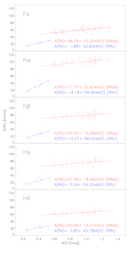
Figure 15: Left-top: difference between radial velocity amplitudes based on Mg and Fe group RVC templates. The mean difference is labeled at the top-right corner. Left-Middle: same as left-top, but for Na and Fe group RVC templates. Left-Bottom: same as the left-top, but between the BW sample and the Fe group RVC templates. Right panels: From top to bottom, visual amplitude ($Amp(V)$) versus radial velocity amplitudes ($Amp(RV)$) based on Fe, H_α, H_β, H_γ and H_δ lines. RRab and RRc variables are marked with red and blue symbols. Uncertainties on $Amp(RV)$ are displayed. Solid lines show the linear relations between $Amp(RV)$ and $Amp(V)$. The analytical form of the relations are labeled at the bottom.

Table 17: Coefficients of the $Amp(RV)$-$Amp(V)$ relations.

	RRc					RRab
Line	a	$e$a	b	$e$b	$\sigma$	a	$e$a	b	$e$b	$\sigma$
	km/s		km/s/mag			km/s		km/s/mag
Fe	1.68	4.92	52.63	12.94	3.50	38.09	2.90	22.35	3.12	4.20
H${\alpha}$	–9.18	9.36	106.69	24.61	6.66	77.77	6.17	22.83	6.64	8.92
H${\beta}$	–0.27	6.92	66.55	18.20	4.93	63.32	4.96	15.96	5.34	7.17
H${\gamma}$	0.54	7.99	59.32	21.02	5.69	57.38	5.01	18.48	5.39	7.24
H${\delta}$	3.85	6.80	45.78	17.88	4.84	50.90	3.84	14.43	4.14	5.55

Note. — Coefficients (a,b), uncertainties ($e$a, $e$b) and standard deviations ($\sigma$) of the $Amp(RV)$ vs $Amp(V)$ relations for RRc and RRab variables.

Appendix B The cumulated radial velocity curves

Figures 16 and 17 display the CNRVCs for all the RVC templates (colored small circles), together with the analytical form of the template (solid line).

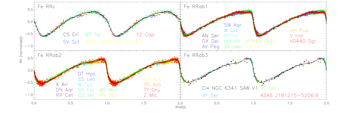
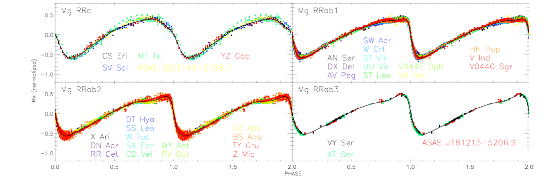
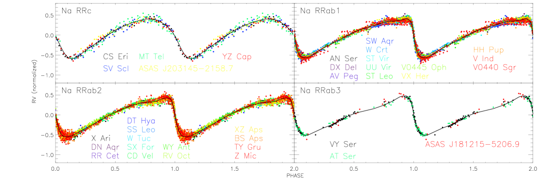
Figure 16: From top to bottom: cumulative and normalized radial velocity curves based on metallic (Fe, Mg, Na) lines. The period bin of the RVC template is labeled on the top left corner. Small circles are color-coded by variables and their names are labeled at the bottom. The solid line displays the analytical form of the RVC templates.

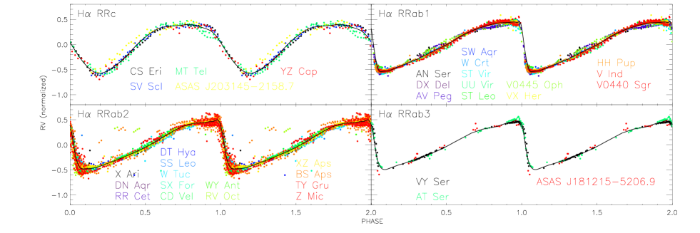
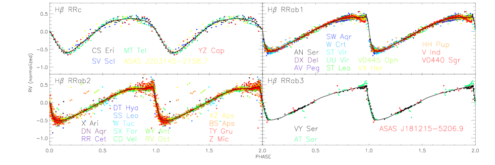
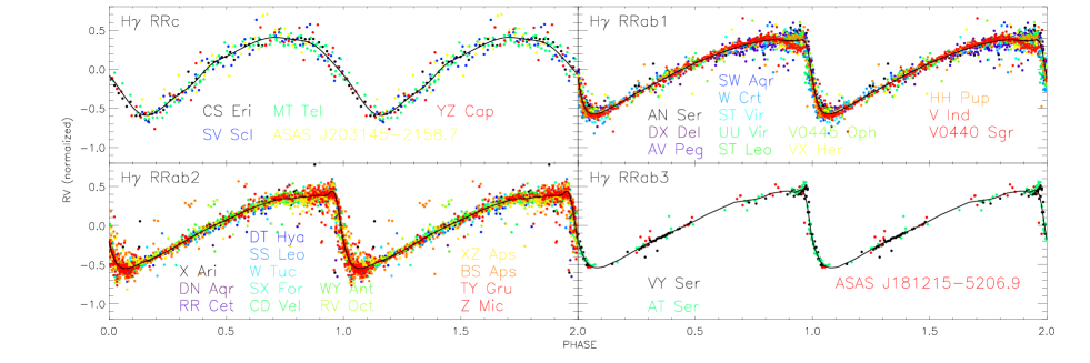
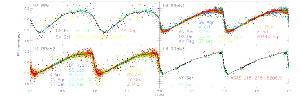
Figure 17: From top to bottom: cumulative and normalized radial velocity curves based on the Balmer (H_α, H_β, H_γ, H_δ) lines. The period bin of the RVC template bin is labeled on the top left corner. Small circles are color-coded by variables and their names are labeled at the bottom. The solid line displays the analytical form of the RVC templates.

By inspecting the CNRVCs it is clear that, within the bins RRab1 and RRab2, the morphology of the RVCs is, on a first approximation, dichotomic. More specifically, within the RRab1 bin, SW Aqr, ST Leo, VX Her, V Ind and V0440 Sgr display a local maximum around the phase 0.70-0.75, instead of the more or less steady rising behavior of the other RRab1 RRLs. Moreover, TY Gru, CD Vel and SX For (RRab2 bin), do not display a local minimum around phase 0.7-0.8, as the other RRab2 variables do. This happens for all the diagnostics, although it is more evident for the Balmer lines. We remark that these features are also present in the optical light curves of these stars.

We checked whether these features can be associated with either pulsation or physical properties of the stars. While it is true that the RRab1 variables with a more prominent local maximum are located in the High-Amplitude Short-Period (HASP, Fiorentino et al. 2015) region, they are not the only HASP variables in our sample. Their iron abundances range between –1.9 and –1.4, which is around the peak of the distribution of field RRLs (Crestani et al. 2021a) and it was not even possible to constrain a morphological class of RVCs based on the Fourier parameters R2, R31, $\phi_{21}$ and $\phi_{31}$ of their light curve.

To sum up, there is no quantitative way to predict, either from the light curve or from the physical properties, which is the RVC morphology of RRab1 and RRab2. This has several consequences: the first and most obvious is that we cannot split these bins and provide more RVC templates because we cannot provide criteria for using one or the other. This may seem to be a disadvantage, but luckily, this dichotomy introduces a $\lesssim$5 km/s offset in the estimate of $V_{\gamma}$ with a probability of $\sim$10-15% (i.e., the fraction of pulsation cycle where the RVCs have a different behavior).

Appendix C How to use the new RVC templates

In this section of the Appendices, we provide precise instructions on how to use the new RVC templates with the aim of estimating V_γ in different realistic cases: $i)$— when only one RV measurement and a well-sampled light curve that allows the estimate of the reference epoch are available; $ii)$— when a few (we assume three) RV measurement and a well-sampled light curve that allows the estimate of the reference epoch are available; $iii)$— when a few (we assume three) RV measurement and a light curve that does not allow an accurate estimate of the reference epoch are available.

C.1 Estimate of $T_{mean}^{opt}$

Before describing how to use the templates, we want to instruct the reader on how to derive $T_{mean}^{opt}$, which is not as common as $T_{max}^{opt}$, therefore it might not be straightforward to estimate.

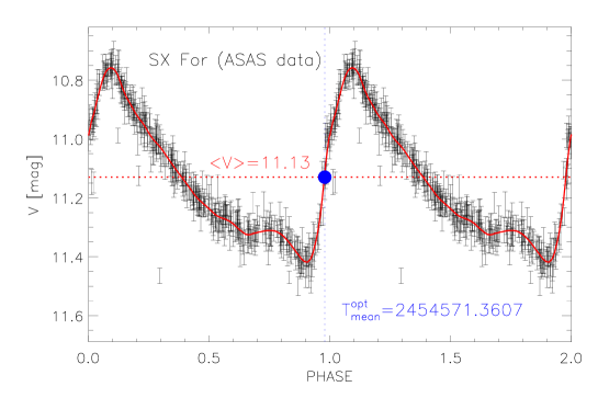
Figure 18: $V$-band ASAS light curve of SX For. The solid red line displays the fitting model. The dashed red line represents the mean magnitude and the blue circle displays the position of $T_{mean}^{opt}$. The values of the mean magnitude and $T_{mean}^{opt}$are labeled in red and blue, respectively.

First of all, the light curve must be phased to an arbitrary reference epoch, e.g., HJD=0, as in Figure 18. Then, the phased light curve must be fit with a model. It is crucial that the model fits well the rising branch. After that, $<V>$ is derived by converting each point of the model into arbitrary flux ($F=10^{-0.4*mag}$), integrating the flux model and finding the mean flux $<F>$ and converting back to magnitude ($<V>=-2.5\cdot\log_{10}(<F>)$).

If the model is analytical (e.g., Fourier or PEGASUS), one can easily find the phase on the rising branch at which the model intersects $<V>$, namely, $\phi_{mean}$. If the model is not analytical (e.g., spline or PLOESS), it is necessary to interpolate $<V>$ with the model sampled on an even grid of phases. A convenient choice for the step of the grid is between 0.001 and 0.01.

Once $\phi_{mean}$ is known, the next step is to select any phase point of the light curve. This will be characterized by an epoch of observation ($t_{V(i)}$, where $i$ indicates the $i$-th point of the light curve) and a phase ($\phi_{V(i)}$). Finally, $T_{mean}^{opt}$= $t_{V(i)}-(\phi_{V(i)}-\phi_{mean})\cdot P$ can be derived.

C.2 Single RV measurement

This is the most classical situation when using any type of template. In this case, only one RV measurement is available. Note that, if the spectral range of the instrument is large enough, it is possible to have one RV measurement per diagnostic (e.g., Fe, Mg and H_γ) but still no more than one epoch is available. This means that any RVC template can be applied to only one point.

The quoted RV measurement consists of an epoch of observation ($t$), a velocity ($RV$) and its uncertainty ($eRV$). In this case, a decent sampling of the light curve is needed, in order to estimate its period ($P$), amplitude ($Amp(V)$), mean magnitude ($<V>$) and the reference epoch $T_{max}^{opt}$  or $T_{mean}^{opt}$.

The first step is to anchor the RV measurement to the same reference epoch as the template. As demonstrated in the body of the paper, it is possible to assume $T_{mean}^{opt}$= $T_{mean}^{RV(Fe)}$  and derive the phase as $\phi=\dfrac{t-T_{mean}^{opt}}{P}\bmod{1}$. If only $T_{max}^{opt}$  estimates are available, as is often the case of data releases of large surveys, it is necessary to derive the phase anchored to $T_{max}^{opt}$  and then apply the offsets provided in Section 2.2: $\phi_{max}=\dfrac{t-T_{max}^{opt}}{P}\bmod{1}$ and then $\phi=\phi_{max}+0.223$ for RRc variables or $\phi=\phi_{max}+0.043+0.099\cdot P$ for RRab variables. In this case, an uncertainty must be associated with $\phi$, namely, the $\sigma$ of the quoted relations: 0.036 for RRc and 0.024 for RRab. By using $\phi$, the RV measurement is now anchored to the same reference of metallic (Fe, Mg, Na) templates. If, however, the RV measurement is from a Balmer line, it is necessary to convert $\phi$ by using the relation provided in Figure 12, that is $\phi_{H\beta}=\phi+0.023-0.096*P$.

The second step is to rescale of the normalized template. For this end, it suffices to convert $Amp(V)$ into $Amp(RV)$ by using the relations provided in Table 17.

The third step is to derive the analytical form of the template both rescaled by $Amp(RV)$ and shifted in zero-point to pass through the RV measurement. For this step, the right coefficients for the RVC template must be selected from Table 10. Afterwards, these coefficients are substituted into Equation 1 to calculate the value of the template (T($\phi$)) at the phase $\phi$. Finally, V_γ is obtained as V_γ=$RV-Amp(RV)\cdot T(\phi)$.

Of course, if RV measurements are available for more than one diagnostic, the quoted steps can be separately applied to all the diagnostics, providing multiple V_γ estimates that can be averaged.

C.3 Multiple RV measurement with reference epoch

In this case, more than one RV measurement per diagnostic and a light curve enough well-sampled are available. The procedure is qualitatively identical to that described in C.2, but having more than one RV measurement per diagnostic allows the averaging of the V_γ estimates for the same diagnostic. Also in this case, if RV measurements are available for more than one diagnostic, these can be averaged to constrain V_γ on a broader statistical basis.

In principle, this method could be applied to any number of RV measurements. However, when these are ten-twelve (or more) and they are more or less evenly sampled, with a good knowledge of the period, it is possible to just fit the points and directly derive a V_γ estimate as accurate as the template itself, or even more if the variable has experienced some phase drift or period change during the time elapsed from the collection of light curve and RV data.

C.4 Multiple RV measurement without reference epoch

In this case, more than two RV measurements per diagnostic are available, but the light curve is only modestly sampled. This means that period and $Amp(V)$ can be estimated from photometric data, but the reference epoch cannot. In this situation, the templates can be used as fitting curves.

This approach is qualitatively different from the other two because one does not have to anchor the template but to fit it to the data. The steps are the following

First of all, phases must be derived by adopting an arbitrary reference epoch $T_{0}$ (e.g., $T_{0}$=0 or $T_{0}$=2,400,000) $\phi=\dfrac{t-T_{0}}{P}\bmod{1}$. Still, if one wants to use the Balmer templates, the conversion $\phi_{H\beta}=\phi+0.023-0.096*P$ must be applied.

Secondly, $Amp(V)$ has to be rescaled into $Amp(RV)$ by using the relations provided in Table 17. This step is analogous to that described in C.2.

The third step, is the selection of the RVC template coefficients from Table 10 and perform a $\chi^{2}$ minimization when fitting the RV data with Equation 2. The minimization must be performed on the two free paramaters $\Delta\phi$ (a horizontal shift) and $\Delta V_{\gamma}$, while all the others remain fixed.

Finally, V_γ is simply derived by integrating the final analytical form of Equation 2. Also in this case, if RV measurements are available for more than one diagnostic, these can be averaged to constrain V_γ on a broader statistical basis.

Appendix D Phase-gridded templates

The anonymous referee suggested that reader might be interested in using analytical functions different from PEGASUS series to apply to RVC templates. To facilitate the independent readers we list, in Table 18, the phase-gridded values of the RVC templates by using the coefficients of the PEGASUS series given in Table 10. the reader can fit these gridded values with any analytical function and use them one to apply the RVC template. We adopted a step of 0.01, This means 101 points per template. We have checked that, for a Fourier series of tenth-to-fifteenth order, this step in phase provides a very good fit of the gridded points. In passing, we stress that these phase-gridded values should not be used in substitution of the analytical templates, but to derive alternative analytical forms of the RVC templates. This is recommended for the single phase point approach and necessary for the multiple phase point approach.

Table 18: Phase-gridded RVC templates.

Species	Template bin	Phase	Template value
Fe	0	0.000	0.0176
Fe	0	0.001	0.0124
Fe	0	0.002	0.0072
Fe	0	0.003	0.0019
Fe	0	0.004	–0.0036
Fe	0	0.005	–0.0092
Fe	0	0.006	–0.0148
Fe	0	0.007	–0.0206
Fe	0	0.008	–0.0265
Fe	0	0.009	–0.0325

Note. — Only ten lines are listed. The machine-readable version of this table is available online on the CDS.

References

- Aguado et al. (2019) Aguado, D. S., Ahumada, R., Almeida, A., et al. 2019, ApJS, 240, 23, doi: 10.3847/1538-4365/aaf651
- Arellano Ferro et al. (2014) Arellano Ferro, A., Ahumada, J. A., Calderón, J. H., & Kains, N. 2014, Rev. Mexicana Astron. Astrofis., 50, 307. https://arxiv.org/abs/1406.2635
- Baade (1926) Baade, W. 1926, Astronomische Nachrichten, 228, 359, doi: 10.1002/asna.19262282003
- Baade (1956) —. 1956, PASP, 68, 5, doi: 10.1086/126870
- Belokurov et al. (2018) Belokurov, V., Deason, A. J., Koposov, S. E., et al. 2018, MNRAS, 477, 1472, doi: 10.1093/mnras/sty615
- Benkő et al. (2021) Benkő, J. M., Sódor, Á., & Pál, A. 2021, MNRAS, 500, 2554, doi: 10.1093/mnras/staa3452
- Bonaca & Hogg (2018) Bonaca, A., & Hogg, D. W. 2018, ApJ, 867, 101, doi: 10.3847/1538-4357/aae4da
- Bono et al. (1997) Bono, G., Caputo, F., Cassisi, S., Incerpi, R., & Marconi, M. 1997, ApJ, 483, 811, doi: 10.1086/304284
- Bono et al. (2003) Bono, G., Caputo, F., Castellani, V., et al. 2003, MNRAS, 344, 1097, doi: 10.1046/j.1365-8711.2003.06878.x
- Bono et al. (1994) Bono, G., Caputo, F., & Stellingwerf, R. F. 1994, ApJ, 432, L51, doi: 10.1086/187509
- Bono & Cassisi (1999) Bono, G., & Cassisi, S. 1999, in Astronomical Society of the Pacific Conference Series, Vol. 165, The Third Stromlo Symposium: The Galactic Halo, ed. B. K. Gibson, R. S. Axelrod, & M. E. Putman, 290. https://arxiv.org/abs/astro-ph/9811175
- Bono et al. (2020a) Bono, G., Braga, V. F., Crestani, J., et al. 2020a, ApJ, 896, L15, doi: 10.3847/2041-8213/ab9538
- Bono et al. (2020b) Bono, G., Braga, V. F., Fiorentino, G., et al. 2020b, A&A, 644, A96, doi: 10.1051/0004-6361/202038191
- Braga et al. (2018) Braga, V. F., Bhardwaj, A., Contreras Ramos, R., et al. 2018, A&A, 619, A51, doi: 10.1051/0004-6361/201833538
- Braga et al. (2015) Braga, V. F., Dall’Ora, M., Bono, G., et al. 2015, ApJ, 799, 165, doi: 10.1088/0004-637X/799/2/165
- Braga et al. (2016) Braga, V. F., Stetson, P. B., Bono, G., et al. 2016, AJ, 152, 170, doi: 10.3847/0004-6256/152/6/170
- Braga et al. (2019) —. 2019, A&A, 625, A1, doi: 10.1051/0004-6361/201834893
- Braga et al. (2020) Braga, V. F., Bono, G., Fiorentino, G., et al. 2020, A&A, 644, A95, doi: 10.1051/0004-6361/202039145
- Buder et al. (2018) Buder, S., Asplund, M., Duong, L., et al. 2018, MNRAS, 478, 4513, doi: 10.1093/mnras/sty1281
- Cacciari et al. (1987) Cacciari, C., Clementini, G., Prevot, L., et al. 1987, A&AS, 69, 135
- Carney et al. (1992) Carney, B. W., Storm, J., & Jones, R. V. 1992, ApJ, 386, 663, doi: 10.1086/171047
- Carollo et al. (2007) Carollo, D., Beers, T. C., Lee, Y. S., et al. 2007, Nature, 450, 1020, doi: 10.1038/nature06460
- Castor (1971) Castor, J. I. 1971, ApJ, 166, 109, doi: 10.1086/150945
- Catelan (2009) Catelan, M. 2009, Ap&SS, 320, 261, doi: 10.1007/s10509-009-9987-8
- Catelan et al. (2004) Catelan, M., Pritzl, B. J., & Smith, H. A. 2004, ApJS, 154, 633, doi: 10.1086/422916
- Clementini et al. (1990) Clementini, G., Cacciari, C., & Lindgren, H. 1990, A&AS, 85, 865
- Clementini et al. (2019) Clementini, G., Ripepi, V., Molinaro, R., et al. 2019, A&A, 622, A60, doi: 10.1051/0004-6361/201833374
- Conroy et al. (2021) Conroy, C., Naidu, R. P., Garavito-Camargo, N., et al. 2021, arXiv e-prints, arXiv:2104.09515. https://arxiv.org/abs/2104.09515
- Crestani et al. (2021a) Crestani, J., Fabrizio, M., Braga, V. F., et al. 2021a, ApJ, 908, 20, doi: 10.3847/1538-4357/abd183
- Crestani et al. (2021b) Crestani, J., Braga, V. F., Fabrizio, M., et al. 2021b, arXiv e-prints, arXiv:2104.08113. https://arxiv.org/abs/2104.08113
- Dalton et al. (2012) Dalton, G., Trager, S. C., Abrams, D. C., et al. 2012, in Ground-based and Airborne Instrumentation for Astronomy IV, ed. I. S. McLean, S. K. Ramsay, & H. Takami, Vol. 8446, International Society for Optics and Photonics (SPIE), 220 – 231, doi: 10.1117/12.925950
- de Jong et al. (2012) de Jong, R. S., Bellido-Tirado, O., Chiappini, C., et al. 2012, in Ground-based and Airborne Instrumentation for Astronomy IV, ed. I. S. McLean, S. K. Ramsay, & H. Takami, Vol. 8446, International Society for Optics and Photonics (SPIE), 252 – 266, doi: 10.1117/12.926239
- Deason et al. (2011) Deason, A. J., Belokurov, V., & Evans, N. W. 2011, MNRAS, 416, 2903, doi: 10.1111/j.1365-2966.2011.19237.x
- Drake et al. (2009) Drake, A. J., Djorgovski, S. G., Mahabal, A., et al. 2009, ApJ, 696, 870, doi: 10.1088/0004-637X/696/1/870
- Drake et al. (2017) Drake, A. J., Djorgovski, S. G., Catelan, M., et al. 2017, MNRAS, 469, 3688, doi: 10.1093/mnras/stx1085
- Duong et al. (2019) Duong, L., Asplund, M., Nataf, D. M., et al. 2019, MNRAS, 486, 3586, doi: 10.1093/mnras/stz1104
- Eggen (1962) Eggen, O. J. 1962, PASP, 74, 159, doi: 10.1086/127779
- Fabrizio et al. (2019) Fabrizio, M., Bono, G., Braga, V. F., et al. 2019, ApJ, 882, 169, doi: 10.3847/1538-4357/ab3977
- Fernley et al. (1990) Fernley, J. A., Skillen, I., Jameson, R. F., et al. 1990, MNRAS, 247, 287
- Ferraro et al. (2018) Ferraro, F. R., Mucciarelli, A., Lanzoni, B., et al. 2018, ApJ, 860, 50, doi: 10.3847/1538-4357/aabe2f
- Fiorentino et al. (2015) Fiorentino, G., Bono, G., Monelli, M., et al. 2015, ApJ, 798, L12, doi: 10.1088/2041-8205/798/1/L12
- For et al. (2011) For, B.-Q., Sneden, C., & Preston, G. W. 2011, ApJS, 197, 29, doi: 10.1088/0067-0049/197/2/29
- Gaia Collaboration et al. (2016) Gaia Collaboration, Prusti, T., de Bruijne, J. H. J., et al. 2016, A&A, 595, A1, doi: 10.1051/0004-6361/201629272
- Gardner et al. (2006) Gardner, J. P., Mather, J. C., Clampin, M., et al. 2006, Space Sci. Rev., 123, 485, doi: 10.1007/s11214-006-8315-7
- Giesers et al. (2019) Giesers, B., Kamann, S., Dreizler, S., et al. 2019, A&A, 632, A3, doi: 10.1051/0004-6361/201936203
- Hajdu et al. (2021) Hajdu, G., Pietrzyński, G., Jurcsik, J., et al. 2021, arXiv e-prints, arXiv:2105.03750. https://arxiv.org/abs/2105.03750
- Helmi et al. (2018) Helmi, A., Babusiaux, C., Koppelman, H. H., et al. 2018, Nature, 563, 85, doi: 10.1038/s41586-018-0625-x
- Helmi et al. (1999) Helmi, A., White, S. D. M., de Zeeuw, P. T., & Zhao, H. 1999, Nature, 402, 53, doi: 10.1038/46980
- Hobart et al. (1991) Hobart, M. A., Pena, J. H., & Peniche, R. 1991, Rev. Mexicana Astron. Astrofis., 22, 275
- Hubble (1926) Hubble, E. P. 1926, ApJ, 64, 321, doi: 10.1086/143018
- Inno et al. (2015) Inno, L., Matsunaga, N., Romaniello, M., et al. 2015, A&A, 576, A30, doi: 10.1051/0004-6361/201424396
- Jayasinghe et al. (2019) Jayasinghe, T., Stanek, K. Z., Kochanek, C. S., et al. 2019, MNRAS, 485, 961, doi: 10.1093/mnras/stz444
- Jones et al. (1988a) Jones, R. V., Carney, B. W., & Latham, D. W. 1988a, ApJ, 326, 312, doi: 10.1086/166093
- Jones et al. (1988b) —. 1988b, ApJ, 332, 206, doi: 10.1086/166647
- Jones et al. (1987a) Jones, R. V., Carney, B. W., Latham, D. W., & Kurucz, R. L. 1987a, ApJ, 314, 605, doi: 10.1086/165090
- Jones et al. (1987b) —. 1987b, ApJ, 312, 254, doi: 10.1086/164867
- Joy (1939) Joy, A. H. 1939, ApJ, 89, 356, doi: 10.1086/144060
- Keller et al. (2008) Keller, S. C., Murphy, S., Prior, S., DaCosta, G., & Schmidt, B. 2008, ApJ, 678, 851, doi: 10.1086/526516
- Kervella et al. (2019) Kervella, P., Gallenne, A., Evans, N. R., et al. 2019, A&A, 623, A117, doi: 10.1051/0004-6361/201834211
- Kinman et al. (2012) Kinman, T. D., Cacciari, C., Bragaglia, A., Smart, R., & Spagna, A. 2012, MNRAS, 422, 2116, doi: 10.1111/j.1365-2966.2012.20747.x
- Kraft & Ivans (2003) Kraft, R. P., & Ivans, I. I. 2003, PASP, 115, 143, doi: 10.1086/345914
- Kunder et al. (2020) Kunder, A., Pérez-Villegas, A., Rich, R. M., et al. 2020, AJ, 159, 270, doi: 10.3847/1538-3881/ab8d35
- Layden (1994) Layden, A. C. 1994, AJ, 108, 1016, doi: 10.1086/117132
- Layden (1995) —. 1995, AJ, 110, 2288, doi: 10.1086/117690
- Layden & Sarajedini (2003) Layden, A. C., & Sarajedini, A. 2003, AJ, 125, 208, doi: 10.1086/344948
- Liu (1991) Liu, T. 1991, PASP, 103, 205, doi: 10.1086/132809
- Liu & Janes (1989) Liu, T., & Janes, K. A. 1989, ApJS, 69, 593, doi: 10.1086/191322
- Liu & Janes (1990) —. 1990, ApJ, 354, 273, doi: 10.1086/168688
- Longmore et al. (1986) Longmore, A. J., Fernley, J. A., & Jameson, R. F. 1986, MNRAS, 220, 279, doi: 10.1093/mnras/220.2.279
- Magurno et al. (2018) Magurno, D., Sneden, C., Braga, V. F., et al. 2018, ApJ, 864, 57, doi: 10.3847/1538-4357/aad4a3
- Majewski et al. (2017) Majewski, S. R., Schiavon, R. P., Frinchaboy, P. M., et al. 2017, AJ, 154, 94, doi: 10.3847/1538-3881/aa784d
- Massari et al. (2019) Massari, D., Koppelman, H. H., & Helmi, A. 2019, A&A, 630, L4, doi: 10.1051/0004-6361/201936135
- Minniti et al. (2011) Minniti, D., Hempel, M., Toledo, I., et al. 2011, A&A, 527, A81, doi: 10.1051/0004-6361/201015795
- Monachesi et al. (2019) Monachesi, A., Gómez, F. A., Grand, R. J. J., et al. 2019, MNRAS, 485, 2589, doi: 10.1093/mnras/stz538
- Moore (1972) Moore, C. E. 1972, A multiplet table of astrophysical interest - Pt.1: Table of multiplets - Pt.2: Finding list of all lines in the table of multiplets
- Mucciarelli et al. (2014) Mucciarelli, A., Lovisi, L., Ferraro, F. R., et al. 2014, ApJ, 797, 43, doi: 10.1088/0004-637X/797/1/43
- Mullen et al. (2021) Mullen, J. P., Marengo, M., Martínez-Vázquez, C. E., et al. 2021, The Astrophysical Journal, 912, 144, doi: 10.3847/1538-4357/abefd4
- Myeong et al. (2018) Myeong, G. C., Evans, N. W., Belokurov, V., Sanders, J. L., & Koposov, S. E. 2018, ApJ, 863, L28, doi: 10.3847/2041-8213/aad7f7
- Oke (1966) Oke, J. B. 1966, ApJ, 145, 468, doi: 10.1086/148787
- Oort (1927) Oort, J. H. 1927, Bull. Astron. Inst. Netherlands, 3, 275
- Piersimoni et al. (2002) Piersimoni, A. M., Bono, G., & Ripepi, V. 2002, AJ, 124, 1528, doi: 10.1086/341821
- Pietrukowicz et al. (2015) Pietrukowicz, P., Kozłowski, S., Skowron, J., et al. 2015, ApJ, 811, 113, doi: 10.1088/0004-637X/811/2/113
- Pietrzyński et al. (2012) Pietrzyński, G., Thompson, I. B., Gieren, W., et al. 2012, Nature, 484, 75, doi: 10.1038/nature10966
- Pojmanski (1997) Pojmanski, G. 1997, Acta Astron., 47, 467
- Prudil et al. (2021) Prudil, Z., Hanke, M., Lemasle, B., et al. 2021, arXiv e-prints, arXiv:2102.01090. https://arxiv.org/abs/2102.01090
- Riess et al. (2019) Riess, A. G., Casertano, S., Yuan, W., Macri, L. M., & Scolnic, D. 2019, ApJ, 876, 85, doi: 10.3847/1538-4357/ab1422
- Searle & Zinn (1978) Searle, L., & Zinn, R. 1978, ApJ, 225, 357, doi: 10.1086/156499
- Sesar (2012) Sesar, B. 2012, AJ, 144, 114, doi: 10.1088/0004-6256/144/4/114
- Sesar et al. (2011) Sesar, B., Jurić, M., & Ivezić, Ž. 2011, ApJ, 731, 4, doi: 10.1088/0004-637X/731/1/4
- Sesar et al. (2010) Sesar, B., Ivezić, Ž., Grammer, S. H., et al. 2010, ApJ, 708, 717, doi: 10.1088/0004-637X/708/1/717
- Sesar et al. (2017) Sesar, B., Hernitschek, N., Mitrović, S., et al. 2017, AJ, 153, 204, doi: 10.3847/1538-3881/aa661b
- Skillen et al. (1993a) Skillen, I., Fernley, J. A., Stobie, R. S., & Jameson, R. F. 1993a, MNRAS, 265, 301, doi: 10.1093/mnras/265.2.301
- Skillen et al. (1993b) Skillen, I., Fernley, J. A., Stobie, R. S., Marang, F., & Jameson, R. F. 1993b, South African Astronomical Observatory Circular, 15, 90
- Smolec et al. (2013) Smolec, R., Pietrzyński, G., Graczyk, D., et al. 2013, MNRAS, 428, 3034, doi: 10.1093/mnras/sts258
- Sneden et al. (2017) Sneden, C., Preston, G. W., Chadid, M., & Adamów, M. 2017, ApJ, 848, 68, doi: 10.3847/1538-4357/aa8b10
- Soszyński et al. (2019) Soszyński, I., Udalski, A., Wrona, M., et al. 2019, Acta Astron., 69, 321, doi: 10.32023/0001-5237/69.4.2
- Spergel et al. (2015) Spergel, D., Gehrels, N., Baltay, C., et al. 2015, arXiv e-prints. https://arxiv.org/abs/1503.03757
- Steinmetz et al. (2006) Steinmetz, M., Zwitter, T., Siebert, A., et al. 2006, AJ, 132, 1645, doi: 10.1086/506564
- Stetson et al. (2014) Stetson, P. B., Braga, V. F., Dall’Ora, M., et al. 2014, PASP, 126, 521, doi: 10.1086/677195
- Stringer et al. (2019) Stringer, K. M., Long, J. P., Macri, L. M., et al. 2019, AJ, 158, 16, doi: 10.3847/1538-3881/ab1f46
- Su et al. (1998) Su, D. Q., Cui, X., Wang, Y., & Yao, Z. 1998, in Society of Photo-Optical Instrumentation Engineers (SPIE) Conference Series, Vol. 3352, Advanced Technology Optical/IR Telescopes VI, ed. L. M. Stepp, 76–90, doi: 10.1117/12.319250
- Tamura et al. (2018) Tamura, N., Takato, N., Shimono, A., et al. 2018, in Society of Photo-Optical Instrumentation Engineers (SPIE) Conference Series, Vol. 10702, Ground-based and Airborne Instrumentation for Astronomy VII, ed. C. J. Evans, L. Simard, & H. Takami, 107021C, doi: 10.1117/12.2311871
- Taylor et al. (2018) Taylor, W., Cirasuolo, M., Afonso, J., et al. 2018, in Ground-based and Airborne Instrumentation for Astronomy VII, ed. C. J. Evans, L. Simard, & H. Takami, Vol. 10702, International Society for Optics and Photonics (SPIE), 421 – 440, doi: 10.1117/12.2313403
- Vasiliev (2019) Vasiliev, E. 2019, MNRAS, 484, 2832, doi: 10.1093/mnras/stz171
- Vasiliev & Baumgardt (2021) Vasiliev, E., & Baumgardt, H. 2021, arXiv e-prints, arXiv:2102.09568. https://arxiv.org/abs/2102.09568
- Wan et al. (2021) Wan, Z., Oliver, W. H., Baumgardt, H., et al. 2021, MNRAS, 502, 4513, doi: 10.1093/mnras/stab306
- Wesselink (1946) Wesselink, A. J. 1946, Bull. Astron. Inst. Netherlands, 10, 91
- Wright et al. (2010) Wright, E. L., Eisenhardt, P. R. M., Mainzer, A. K., et al. 2010, AJ, 140, 1868, doi: 10.1088/0004-6256/140/6/1868
- Xue et al. (2015) Xue, X.-X., Rix, H.-W., Ma, Z., et al. 2015, ApJ, 809, 144, doi: 10.1088/0004-637X/809/2/144
- Yanny et al. (2009) Yanny, B., Rockosi, C., Newberg, H. J., et al. 2009, AJ, 137, 4377, doi: 10.1088/0004-6256/137/5/4377
- Zinn et al. (2020) Zinn, R., Chen, X., Layden, A. C., & Casetti-Dinescu, D. I. 2020, MNRAS, 492, 2161, doi: 10.1093/mnras/stz3580