Topological invariance in whiteness optimisation

Abstract

Increasing the light scattering efficiency of nanostructured materials is becoming an active field of research both in fundamental science and commercial applications. In this context, the challenge is to use inexpensive organic materials that come with a lower refractive index than currently used mineral nanoparticles, which are under increased scrutiny for their toxicity. Although several recent investigations have reported different disordered systems to optimise light scattering by morphological design, no systematic studies comparing and explaining how different topological features contribute to optical properties have been reported yet. Using in silico synthesis and numerical simulations, we demonstrate that the reflectance is primarily determined by second order statistics. While remaining differences are explained by surface area and integrated mean curvature, an equal reflectance can be obtained by further tuning the structural anisotropy. Our results suggest a topological invariance for light scattering, demonstrating that any disordered system can be optimised for whiteness.

Introduction

Light diffusion in random structures is a fairly well established phenomenon that has a profound impact in fundamental research as well for applications: from random lasing to light harvesting to imaging and white paints.[1, 2] In fact, bright whiteness is typical of materials where light undergoes multiple scattering events over a broad range of wavelengths. Such diffusive reflectance usually requires high refractive index media (with related safety concerns [3]) or thick scattering layers to ensure sufficient amount of scattering events. Recently, natural examples of disordered materials have drawn much attention due to their ability to express record transport mean free path using low refractive index components. In particular, the white beetles, e.g. Lepioda stigma and Cyphochilus sp. – which exploit an anisotropic chitin network ($n_{c}\approx 1.55$) to achieve a bright whiteness – have become the poster children of disordered photonics[4, 5, 6, 7, 8, 9]. Several investigations have attributed these optical properties to the specific characteristics of the random network structure of the materials. However, due to limited ”metrics” used to compare and analyse random structures, the role of the various features of these complex nanostructures in the scattering properties remains still unclear.

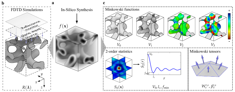
Figure 1: Workflow model of the disorder optics investigations. a A disordered structure, $f(\mathbf{x})$, is synthesised using stochastic model in silico, and b imported to finite difference time domain (FDTD) optics simulator with periodic boundary conditions in $x$- and $y$-directions and a plane wave propagating along $z$ to obtain broad band reflectance spectra, $R(\boldsymbol{\lambda})$. c The optical results are investigated in respect to structural descriptors which include second order statistical measures such as 2-point correlation functions $S(r)$, filling fraction $V_{0}$, and correlation length $l_{c}$, but also more unique structural measures like Minkowski functionals, $V_{0},V_{1},V_{2},V_{3}$ which are the integrated volume, surface area, mean and Gaussian curvatures respectively (colours represent piecewise contributions), and also Minkowski tensors $W^{r,s}_{\nu}$, and the associated eigenvalue ratios $\beta^{r,s}_{\nu}$ which measure the structural anisotropy.

Disordered systems are loosely defined as inhomogeneous materials that exhibit small (but not long range) structural correlations at relevant length distances $\mathbf{r}$. The most popular measures used to characterise disordered systems in optics are based on first and second order statistics such as form- and structure factors, 2-point correlation function $S_{2}(\mathbf{r)}$, filling fraction, $V_{0}(:=S_{2}(0))$, and correlation length $l_{c}$. It has been suggested that unique structural similarities between disordered systems can be inferred from identical reflectance spectra $R(\lambda)$ and $S_{2}(r)$[10]. Yet in the case of random network structures inspired by white beetles, many different synthetic models have been reported to match the beetle structures using these functionals [11, 12, 10, 13], suggesting its non-uniqueness. This is not surprising, given that in the field of disordered studies, which predates the study of disordered photonics, it is well known that only in few exceptions, e.g. in the case Gaussian random fields, also known as Gaussian Processes (GP), the structural properties of stochastic fields are uniquely determined by second order statics alone [14], and for an arbitrary ones more robust topological measures are needed for unique characterisation. Therefore we propose to use a particularly useful metrics for this quantification: the Minkowski functionals $V_{0},V_{1},V_{2},V_{3}$, which are based on surface integrals, and are proportional to the filling fraction, surface area, integrated mean and total curvature respectively [15, 16].

Using such topological identifiers we tested the scattering efficiency of a series of disordered structures synthesised in silico using both top-down and bottom-up models to cover a wide range of topological features in terms of porosity, connectedness, branching and length scale. We quantified these differences using the Minkowski functionals and measured the reflection properties using finite-difference time domain (FDTD) simulations (cf. Fig. 1). Then, by correlating the two, we were able to understand how each feature contributes to overall scattering properties, demonstrating that disordered systems are sufficiently explained by second order statistics alone. Finally using the the tensorial Minkowski measures[17, 18], we also quantified structural anisotropy and investigated its role in whiteness optimisation.

Results

In silico synthesis of disordered structures

As the size of the parameter space for disordered structures is enormous, we selected 10 different model systems (GP1-2, FC1-5, and SD1-3, cf. Figure 2a) using three different stochastic approaches and mapped the reflectivity landscape using line searches by varying i) the correlation length $l_{c}$, ii) filling fraction $V_{0}$ and anisotropy of these systems. We believe that our selection covers a significant wide range of different topological features relevant to the topic of scattering optimisations.

In the first approach we used Gaussian Processes (GPs), which are completely defined by their mean $m(\mathbf{r})$ and $S_{2}(\mathbf{r})$ (the latter is also known as covariance kernel in machine learning literature), to test the dependency of photonic properties of disordered structures on second order statistic alone. We selected two different correlation functions, one with sinc-type and other with squared exponential

$$\text{GP1: }\ \ S_{2}(r)\propto\frac{\sin{(lr)}}{lr},\hskip 42.67912pt\ \text{GP2: }\ \ S_{2}(r)\propto\exp\left(\frac{-r^{2}}{2l^{2}}\right)$$ (1)

where $l$ is a scaling parameter, to investigate the effect of a fixed correlation length, (GP1), vs. one with distribution of correlation lengths (GP2) (cf. Figure 2a), on the optical response.

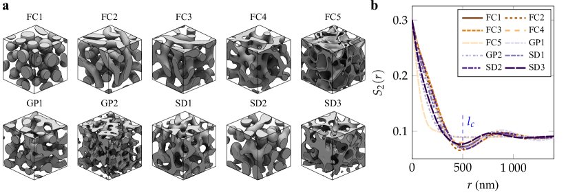
Figure 2: a Investigated simulated structures morphologies including Functionalised Cahn-Hilliard (FC*), Gaussian Processes (GP*), and spinodal decomposition (SD*) using the Cahn-Hilliard model. b The second order correlation functions, $S_{2}(r)$, of these structures demonstrating that very different topologies are often indistinguishable using second order statistics alone.

In the second case, we used a popular phase-field approach, the Cahn-Hilliard (CH) model [19] to generate more complex structures. The CH model successfully describes the time evolution of demixing process (known as spinodal decomposition) of homogeneous mixture into separate domains and was chosen as it has recently been suggested as the formation mechanism behind the beetle scale structures [10]. We used three spinodal decomposition (SD) models, which we initialised using $50\text{\,}\mathrm{\char 37\relax}$, (SD1), $30\text{\,}\mathrm{\char 37\relax}$, (SD2), and $70\text{\,}\mathrm{\char 37\relax}$, (SD3) filling fractions.

Although the CH model has been successfully used to simulate disordered structures in many different fields, it’s mainly limited to bicontinuous networks and isolated micelle morphologies, that exclude the possibility to investigate e.g. tubular and cellular morphologies. A particularly interesting approach, that was developed to gain control over these features, is the Functionalised Cahn-Hilliard (FCH) model [20, 21, 22] which takes into account hydrophobic and mixing entropy effects, allow to control the surface curvature. Therefore in the third approach we adopted a known FCH protocol with $20\text{\,}\mathrm{\char 37\relax}$ initial filling fraction[20], to simulate a variety of structures from colloidal, (FC1), and tubular, (FC2), to branched and cellular (FC3-FC5) ones). These structures are also interesting as they offer flexibility in visual and quantitative (using the $V_{n}$) matching of synthetic disordered systems with biological ones.

FDTD simulations

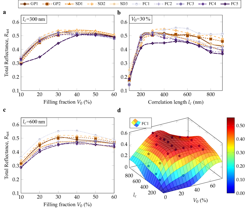
Figure 3: Line searches along different filling fractions $V_{0}$ and correlation lengths $l_{c}$ for different morphologies. a,c Varying filling fraction with fixed $l_{c}=$300\text{\,}\mathrm{n}\mathrm{m}$$ and $l_{c}=$600\text{\,}\mathrm{n}\mathrm{m}$$. b Varying correlation length with fixed $V_{0}=$30\text{\,}\mathrm{\char 37\relax}$$. d) Extrapolated surface for the most reflective system FC1.

.

FDTD simulations were carried out using a broadband plane wave source and a reflectance monitor above the sample. The reflectance spectra were then integrated over the monitor area, and spectrally averaged to obtain total reflectance $R_{\text{tot}}$. Because the parameter space, spanned by correlation length $l_{c}$ and $V_{0}$, is rather large, and the FDTD simulations are computationally relatively costly, we carried out series of line scans by keeping the $l_{c}$ fixed and varying $V_{0}$, and vice versa, for each model.

Starting from $l_{c}=$300\text{\,}\mathrm{n}\mathrm{m}$$ and $V_{0}=30$% one would have expected (under the assumption that optical properties are not solely determined by 2nd order statistics) to see clear difference in reflectivity between different structures. Surprisingly not only were the average reflectances between different structures, very similar, from 0.49 to 0.53, except for the cellular structure FC5 with $R\approx 0.45$, but they all behaved in a similar unimodal manner as function of $V_{0}=[10,20,30,40,50,60]$%, as shown in Figure 3a, with highest reflectivity reached between $V_{0}=$$3050\text{\,}\mathrm{\char 37\relax}$ in agreement with earlier studies[23]. Next, we therefore continue to scan over correlation lengths between $l_{c}=[$100\text{\,}\mathrm{n}\mathrm{m}$,$200\text{\,}\mathrm{n}\mathrm{m}$,\dots,$900\text{\,}\mathrm{n}\mathrm{m}$]$ while keeping the $V_{0}=$30\text{\,}\mathrm{\char 37\relax}$$ fixed, cf. Figure 3b. Here it could be seen that the value $l_{c}=$300\text{\,}\mathrm{n}\mathrm{m}$$ was a convergence point for most structures. When moving to higher values, the differences became more pronounced and in favour of colloidal systems, like FC1 and SD2, and interestingly at the expense of inverse/cellular structures, such as FC5 and SD3. We then line scanned $V_{0}=[10,20,30,40,50,60]$% only to discover similar unimodal behaviour and an optimal region of $V_{0}=$$3040\text{\,}\mathrm{\char 37\relax}$, with the exception of more pronounced separation in averaged reflection between the different structures.

Role of anisotropy

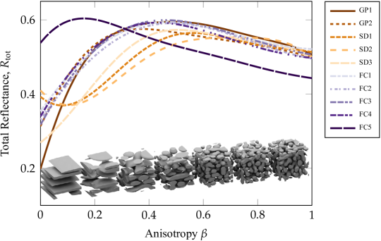
Figure 4: Effect of anisotropy $\beta$ on average reflectance. A value of $\beta=1$ indicates complete structural isotropy and $\beta=0$ full structural anisotropy. The lines present Gaussian Process fits to measured (FDTD simulated) reflectances. The data points have been omitted for clarity, and can be found ESI, Figure S3. Snapshots of FC1 structures are shown in the bottom to illustrate the effect of the anisotropy on a morphology.

As structural anisotropy is known to be an important feature affecting the reflectance properties of disordered systems[24], we decided to use the Minkowski tensors, which are based on strong mathematical foundation of integral and convex geometry[17], to quantitatively correlate the structural anisotropy to the optical response. In fact, to the best of our knowledge, a robust way to quantify the anisotropy of an arbitrary structure[24] is still lacking in the photonics community. Popular methods include the simple comparison of ratios of correlation lengths along different directions, but question how such values should be interpreted remains open, and can be rather inaccurate for latent anisotropy, as we will later demonstrate.

In 3D there are several different linearly-independent tensors, and a particularly suitable one for two-phase structures is

$$W^{0,2}_{1}(I(\mathbf{x})):=\frac{1}{3}\int_{\partial I}\mathbf{n}\otimes\mathbf{n}\ dA$$ (2)

which measures the distribution of surface normals $\mathbf{n}$ [25, 18]. The degree of anisotropy can then be expressed as the ratio of minimal and maximal eigenvalue of the tensor

$$\beta^{0,2}_{1}:=\frac{|\mu_{\min{}}|}{|\mu_{\max{}}|}\in[0,1]$$ (3)

which we will now on referred as $\beta$. An isotropic structure will have $\beta\approx 1$ and lower values signify increased anisotropy.

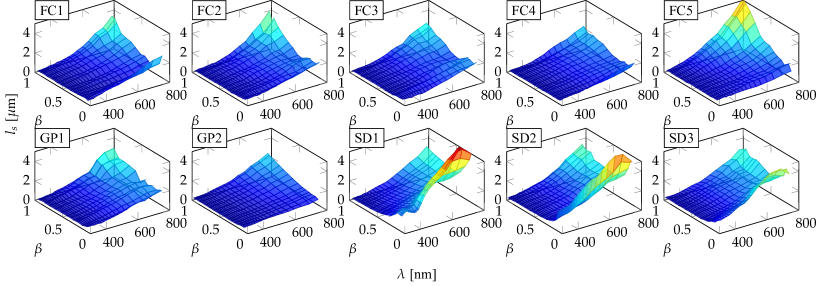
Figure 5: The scattering mean free path, $l_{s}$, as function of wavelength $\lambda$, and anisotropy $\beta$. The plots demonstrate how, especially on large wavelengths, the scattering can be increased with anisotropy optimisation

By replacing the scale parameters and diffusion coefficients in equations (1),(6), and (9) with ones that are independent along different axes we can extending our simulations to model also anisotropic structures [26] and using the Minkowski tensors, we can both induce and quantify structural anisotropy, and therefore systematically map its effect on the photonic response. Thus, for all the model types, we created a series of structures with anisotropy ranging between $\beta\in[0,1]$, while keeping the other parameters, $V_{0}=0.3$ and $l_{c}=$300\text{\,}\mathrm{n}\mathrm{m}$$ fixed. The values of $\beta$ were roughly evenly spaced since a structure with an arbitrary anisotropy value has to be iteratively searched.

The result are shown Figure 4. In all cases the reflectance shows improvement with increasing anisotropy usually peaking to $R\approx 0.6$ between $\beta\in[0.4,0.6]$. It is interesting to note that, thanks to release of the X-ray tomography data sets of the beetle scales to public domain by Burg and coworkers [27], we were also able to precisely quantify that that disordered structures inside both Lepioda stigma and Cyphochilus sp. scales are also anisotropic, $\beta=0.7$ and $\beta=0.6$ respectively. In the latter case there has been some speculation whether the structure is isotropic or not, but the quantitative analysis confirms that the original anisotropy claim [5, 28] is valid. What is most surprising, for the simulated structures, is that the system that shows worst reflectivity in the isotropic case, FC5, reaches the highest reflectivity $R\approx 0.63$ at $\beta\approx 0.15$ among all the models, suggesting that even relatively poor reflectance can be optimised with anisotropy.

One should note that all the structures, at high anisotropy, start to resemble 1D multilayer-like systems, and therefore we would expect them also show high reflectivity due to consistency with literature reports [29]. In the supporting information we demonstrate that correlation lengths are merely shifted and by reoptimisation the higher reflectance levels can be recovered (cf. Figure S2).

Moreover, by comparing mean free paths as function of anisotropy, as shown in Figures 5 (cf. ESI for transport mean free path $l_{t}$) we observed the spectrally averaged mean free paths are rather similar between the different structures, and differences are mostly related to spectral variances. Furthermore these variances are decreased with increasing anisotropy with bottle neck like optima between $\beta\sim 0.2$–$0.7$ suggesting anisotropy plays an important role in whiteness optimisation.

Feature analysis

So far we have mostly related topologically invariant features such filling fraction, correlation length, and anisotropy to reflectance properties. Ultimately one aims to arrive at an analytical model for predicting photonic properties of an arbitrary disorder structure via examining above mentioned structural properties. Deriving such model is very difficult task, and instead a black box approach is needed. Machine Learning (ML) methods have become very popular in such problems. In particular deep learning based (and similar) ML methods are becoming popular for disorder structures investigations in photonics and material science[30, 31], and allow the use of raw 3D structures in the learning process. While those approaches are in principle very powerful in predicting the output (photonic) from the inputs (3D structure), given large enough training dataset, the challenge of interpreting the structure-property relationship between the two remains. Given that we have the various structural descriptors, such as Minkowski functions and anisotropy values, using them instead of the raw 3D structures for ML regression analysis, we can quantitatively estimate the importance of each features, and since each of those features physical interpretation also the inference will be more interpretable.

Thus we simply collect all the relevant structural features (a.k.a labels), for each simulated structure and reflectance spectra $R(\lambda)$, and use regression analysis with the following mapping

$$[l_{c},f_{\min},V_{0},V_{1},V_{2},V_{3},\beta^{2,0}_{0},\beta^{0,2}_{1},\beta^{2,0}_{1},\beta^{2,0}_{2},\beta^{2,0}_{2},\beta^{2,0}_{3},b_{0},b_{1},b_{2}]\to R_{\text{avg}}(\lambda)$$ (4)

where $f_{\min}$ is the correlation strength (cf. ESI), $\beta^{r,s}_{\nu}$ are the anisotropy factors [18], and the Betti numbers $b_{0}$, $b_{1}$, $b_{2}$ measure the number of particles, loops, and cavities respectively [32].

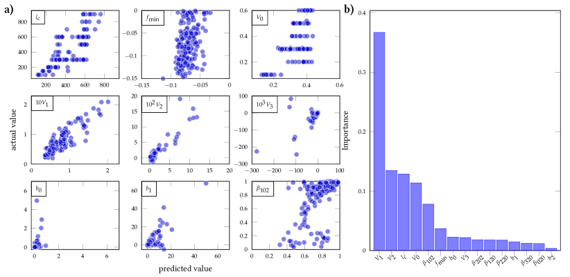
Figure 6: Feature importance analysis using Random Forest regression. a) Plots of predicted and actual values of the various features (Only the 9 most relevant are shown for space considerations). A good correlation between predicted and actual value (diagonal distribution of points) is interpreted to signify high relevance to reflectance. b) Quantitative analysis of the feature importance. Value of 1 signify high and 0 low importance.

A practical way to assess the importance of each feature is to divide the data to training and test sets, and compare how accurately a ML model, trained with former dataset, can predict a particular feature from the latter. Features that are easy to predict correctly can be interpreted to have a higher significance for the output, ($R(\lambda)$), and thus imply a stronger structure-property relationship.

For instance using the popular Random Forest (RF) ML regression model for equation (4), we observed in Figure 6a), that most easily predictable features, from reflectance spectra, are the surface area $V_{1}$, integrated mean curvature $V_{2}$, and correlation length $l_{c}$. Furthermore, using quantitative importance analysis, we can give percentual estimates of importance of each 15 features to reflectivity, with the five most important being $V_{1}$ ($37\text{\,}\mathrm{\char 37\relax}$), $V_{2}$ ($13\text{\,}\mathrm{\char 37\relax}$), $l_{c}$ ($13\text{\,}\mathrm{\char 37\relax}$), $V_{0}$ ($11\text{\,}\mathrm{\char 37\relax}$), $\beta$ ($8\text{\,}\mathrm{\char 37\relax}$). These values should however be taken as tentative, since the importance analysis is rather sensitive parameter limits. E.g. structures with very low filling fractions, $V_{0}<$10\text{\,}\mathrm{\char 37\relax}$$, will have very low reflectance, and including them feature analysis will result in higher weighting of $V_{0}$ in importance, and the same is true for $l_{c}<100$nm. Therefore we performed the feature analysis above these limits, where we still have reasonably amount of reflectance. The suggestion that the surface area $V_{1}$ and the mean curvature $V_{2}$ are the most important features is a consequence of the fact that the colloidal systems (FC1 & SD2) seem to be most reflective. This indicated that disordered assembly of particles would give the highest reflectance. To test this hypothesis we performed series of molecular dynamics particle simulations with the same correlation lengths $l_{c}=$$100900\text{\,}\mathrm{n}\mathrm{m}$. To also check if the reflectance is dependent on the particle shape, we carried out the simulations with both spheres and tetrahedrons, as the latter has a higher integrated mean curvature, due to sharp edges, and increased surface area compared to the former.

The results (cf. ESI, Figure S1) indeed show that the spheres outperform the other systems in reflectivity, whereas tetrahedrons show only moderate reflectance levels, suggesting that the minimal surface area with high mean curvature, under the constrain of filling fraction and correlation length, is a relevant factor for reflectance. Finally, whether spheres are, in general, the optimal shape for particle system in respect to reflectance is interesting but out of the scope of this work.

Conclusion

Using different stochastic models we synthesised, in silico, a diverse set of disordered structures varying in shape, connectiveness, curvature, surface properties, volume, percolation, number of particles and anisotropy. We then measured their reflectance properties, quantified their structural differences, and analysed the structure-property relationships. Our extensively research revealed that all the investigated disordered systems exhibit similar unimodal behaviour in respect to filling fraction and correlations lengths. By utilising the Minkowski measures we were able for the first time quantitatively relate structural features, including anisotropy, to optical properties suggesting that with proper tuning of the second order statistical features ($l_{c}$ and $V_{0}$), and anisotropy brilliant whiteness can be achieved in any system. While colloidal systems have the highest reflectance due their to small surface area $V_{1}$ and high mean curvature $V_{2}$, due to the lack physical support at optimal filling fraction $V_{0}=$$3040\text{\,}\mathrm{\char 37\relax}$, they are not a feasible solution in the context of material fabrication. Therefore whiteness must be realised with continuous structures. However in this case, we observed that choice of particular morphology becomes irrelevant as we have demonstrated. From an industrial and design point of view this is very fortunate, as one is not limited to trying to realise a particular morphology for optimal whiteness, but instead the efforts can be focused on optimising the before mentioned invariant parameters.

The results also suggest that one has to be careful when inferring the about underlying formation mechanism of biological disordered systems using optical response and $S_{2}(r)$ alone, due to non-uniqueness of these characteristics. Conversely this would also explain why there are many different disorder system in nature that exhibit whiteness [33, 34, 35], as the results suggest that any disordered system generated by a tuneable mechanism can be optimised for brilliant whiteness.

In conclusion our work suggests that there is no unique route to brilliant whiteness, and instead it can be realised from many different starting positions.

Methods

All the in silico syntheses were carried out in a $N\times N\times N$ cubic grid with periodic boundary conditions, and set to correspond to a $L^{3}=$$5\text{\,}\mu\mathrm{m}$$\times$$5\text{\,}\mu\mathrm{m}$$\times$$5\text{\,}\mu\mathrm{m}$ box. A value of $N=100$ was used for all structures with $l_{c}\geq$200\text{\,}\mathrm{n}\mathrm{m}$$, and $N=200$ otherwise.

Gaussian processes

The GP1-2 models where synthesised spectrally using fast Fourier transform (FFT) techniques [36, 37, 38, 39]

$$f(\mathbf{x})=\mathbf{S}*\mathbf{N}=\operatorname{FFT}^{-1}\left[\operatorname{FFT}(\mathbf{S})\cdotp\operatorname{FFT}(\mathbf{N})\right]$$ (5)

where $\mathbf{S}=[\mathbf{S}_{1},\dots,\mathbf{S_{N}}]$, $\mathbf{N}=[\mathbf{N}_{1},\dots,\mathbf{N}_{N}]$ are $(N\times N\times N)$ arrays and

$$\mathbf{S}_{k}=\begin{bmatrix}s_{11k}&s_{12k}&\dots&s_{1Nk}\\ s_{21k}&s_{22k}&\dots&s_{2Nk}\\ \vdots&\vdots&\ddots&\vdots\\ s_{N1k}&s_{N2k}s&\dots&s_{NNk}\end{bmatrix},\ \mathbf{N}_{k}=\begin{bmatrix}n_{11k}&n_{12k}&\dots&n_{1Nk}\\ n_{21k}&n_{22k}&\dots&n_{2Nk}\\ \vdots&\vdots&\ddots&\vdots\\ n_{N1k}&n_{N2k}&\dots&n_{NNk}\end{bmatrix},$$

and $s_{ijk}=S_{2}(r_{ijk})$, $r^{2}=(\tfrac{N}{2}-i)^{2}+(\tfrac{N}{2}-j)^{2}+(\tfrac{N}{2}-k)^{2}$, $n_{ijk}\sim\mathcal{N}(0,1)$

Phase-field simulations

The Cahn-Hilliard model used for generating the spinodal decomposition structures SD1-3 is given by

$$\frac{\partial f}{\partial t} =\nabla^{2}M\left[\frac{\partial W(f)}{\partial f}-\tfrac{1}{2}\epsilon(\nabla f)^{2}\right]$$ (6)

$$W(f) =Af^{2}(1-f)^{2}$$ (7)

where $M$ and $\epsilon$ are the mobility and the diffusion constants, and $W(f)$ is the mixing energy between the two equilibrium phases, and was numerically solved using semi-explicit spectral method[40, 41]

$$\mathbf{F}^{[n+1]}=\frac{\mathbf{F}^{[n]}-\Delta tk^{2}MW^{\prime}(\mathbf{F}^{[n]})}{1+\Delta tk^{4}M\epsilon}$$ (8)

where $\mathbf{F}^{[i]}=\operatorname{FFT}(\mathbf{f}^{[i]}),$with time step $\Delta t=1\times 10^{-3}$, $A=1$, $M=1$, and the coefficient $\epsilon$ was chosen from [0.04,1.00] to reach the desired length scale.

The FC1-5 models were created with Functionalised Cahn-Hilliard model [20, 21]

$$\frac{\partial f}{\partial t} =\Delta\left[E_{b}\left(\epsilon^{2}\Delta-W^{\prime\prime}_{b}(f)\right)\left(\epsilon\Delta f-W^{\prime}_{b}(f)\right)+\eta_{h}\epsilon^{2}\Delta f-\eta_{m}W^{\prime}_{s}(f)\right]$$ (9)

$$W_{s}(f) =W_{b}(f)=\frac{1}{2}\left(f+1\right)^{2}\left(\tfrac{1}{2}(f-1)^{2}+\frac{\tau}{3}(f-2)\right).$$ (10)

using the CUDA code of Jones [22] with $\eta_{h}=5$ and $\eta_{m}=[-7.25,-0.5,3,6,10]$ for FC1-5 respectively.

Synthesis of anisotropic structures

Anisotropic structures where synthesis using a the method of Essery [26] where the mobility coefficient $\epsilon$ in equations (6), and (9) was replaced by tensor

$$\epsilon=\begin{bmatrix}\epsilon_{x}&0&0\\ 0&\epsilon_{y}&0\\ 0&0&\epsilon_{z}\end{bmatrix}$$ (11)

and a similar method for the GP models by anisotropic scaling $r^{2}=\epsilon^{2}_{x}(\tfrac{N}{2}-i)^{2}+\epsilon^{2}_{y}(\tfrac{N}{2}-j)^{2}+\epsilon^{2}_{z}(\tfrac{N}{2}-k)^{2}$ in equation (5).

Conversion to binary fields

The stochastic fields $f(\mathbf{x}):\mathbb{R}^{3}\to\mathbb{R}$ synthesised with the different methods were converted to the two phase disordered structures $I(\mathbf{x}):\mathbb{R}^{3}\to\{0,1\}$ using a simple thresholding scheme

$$I(\mathbf{x})=\begin{cases}0,&\text{if }f(\mathbf{x})<p_{0}\\ 1,&\text{else }\end{cases}$$

where $I(\mathbf{x})$ is an indicator function , and $0$ and $1$ represent the empty and the solid phase, respectively, and $p_{0}$ is the threshold value. Thus the final filling fraction $V_{0}=\langle I(\mathbf{x})\rangle$ of structures is determined by the choice of $p_{0}$. While such systems might be physically difficult to realise, we are primarily interested in understanding the optical properties of disorder systems, and question about chemical synthesis of potential structures are beyond the scope of this paper.

For the FDTD simulation, the structures $f(\mathbf{x})$ were imported to USCF chimera [42] and converted to STL stereolitography files using a similar level set scheme.

Particle simulations

The additional particle simulations (see ESI) were conducted with HOOMD-blue[43, 44]package using molecular dynamics simulation with Langevin integrator and Weeks-Chandler-Andersen potential for spheres, and hard particle Monte Carlo simulation for the tetrahedrons.

Calculation of Minkowski measures

The Minkowski functionals of $I(\mathbf{x})$

$$\begin{array}[]{ll}V_{0}(I)=\int_{I}dV,&V_{1}(I)=\frac{1}{3}\int_{\partial I}ds\\ V_{2}(I)=\frac{1}{6}\int_{\partial I}\frac{1}{2}\left(\frac{1}{r_{1}(s)}+\frac{1}{r_{2}(s)}\right)ds,&V_{3}(I)=\frac{1}{3}\int_{\partial I}\frac{1}{r_{1}(s)r_{2}(s)}ds\end{array}$$ (14)

where $r_{1}(s)$ and $r_{2}(s)$ are the maximum and minimum curvature radii [45], the Minkowski tensors $W^{r,s}_{\nu}$ and anisotropy factors

$$\beta^{r,s}_{\nu}:=\frac{|\mu_{\min{}}|}{|\mu_{\max{}}|}\in[0,1],$$ (15)

where $\mu_{\min}$ and $\mu_{\max}$ are the minimal maximal eigenvalue of $W^{r,s}_{\nu}$, were calculated using the Karambola software package [17, 18] from the STL converted files. Anisotropy values for beetle scales were calculated from the files CY_cube.npy and LS_cube.npy of Burg and coworkers’ dataset[27].

Calculation of two-point correlation functions

To determine the characteristic length scale of the simulated structures $I(\mathbf{x})$, we used radially averaged 2-point correlation function calculated using FFT method[46]

$$S_{2}(r)=\frac{\sum_{l,m,n\in\Omega}\operatorname{FFT}^{-1}\left(|\operatorname{FFT}(I(\mathbf{x}))|^{2}\right)}{\omega}$$ (16)

where $\Omega=\left\{(l,m,\ n)\ |\ l^{2}+m^{2}+n^{2}=r^{2},\ r\leq N/2\right\}$ and $\omega$ is the number of elements in $\Omega$. The correlation length, $l_{c}$, was defined to be the distance where 2-point correlation function has its first minima $l_{c}:={\mathrm{argmin}}_{r}\ S_{2}(r)$. For cases where $S_{2}(r)$ was monotonically decreasing we used definition of $l_{c}$ as the minimum distance $r_{n}$ where relative change, $\frac{S_{2}(r_{n})-S_{2}(r_{n+1})}{S_{2}(0)}$ , was less than $0.1\text{\,}\mathrm{\char 37\relax}$. Correlation strength was defined as the relative depth of the minima of $S_{2}(r)$

$$f_{\min}=\min{\left(\frac{S_{2}(r)-S^{2}_{2}(0)}{S_{2}(0)-S_{2}^{2}(0)}\right)}$$ (17)

Finite-difference time domain (FDTD) calculations

The FDTD simulations were carried out using Lumerical 2020a-r5 (Ansys Canada Ltd), with periodic boundary conditions and perfect matching layer boundaries in x, y-directions and broad band source $\lambda\in[300,800]$nm in p-polarisation (TM-mode) coming from vertical direction. The refractive index for the material was set to $n=1.50$ in all cases. The numerical stability and convergence was ensured with the adequate boundary condition and the simulations were carried out until all incoming light had either reflected or transmitted. For the mean free path calculations, the ballistic transmission was recorded using additional TM and TE monitors.

Regression analysis

The feature importance calculations were carried out using RandomForestRegressor of Scikit-learn[47] Python library with 200 trees for features collected from 400 simulated structures.

High performance computations

The FDTD simulations in this work were performed using resources provided by the Cambridge Service for Data Driven Discovery (CSD3) operated by the University of Cambridge Research Computing Service (www.csd3.cam.ac.uk), provided by Dell EMC and Intel using Tier-2 funding from the Engineering and Physical Sciences Research Council (capital grant EP/P020259/1), and DiRAC funding from the Science and Technology Facilities Council (www.dirac.ac.uk).

The in silico synthesis of the FC1-5 structures were performed using computer resources provided by the Aalto University School of Science ”Science-IT” project (https://scicomp.aalto.fi/).

Code and data availability

Matlab code for generating the GP1-2 and SD1-3 structures and $S_{2}(r)$ calculations, and additional data related to this publication is available at the University of Cambridge data repository (https://doi.org/10.17863/CAM.71288).

Author contributions statement

J.S.H did the in silico synthesis and data analysis, G. J and J.S.H carried out the FDTD simulations, J.S.H, G.J, L.S, and S.V designed the experiments, commented on results and wrote the manuscript.

Competing interests

The authors declare no competing interests.

Additional information

Correspondence should be addressed to J.S.H or S.V.

References

- [1] Wiersma, D. S. Disordered photonics. \JournalTitleNature Photonics 7, 188–196, DOI: 10.1038/nphoton.2013.29 (2013).
- [2] Yu, S., Qiu, C.-W., Chong, Y., Torquato, S. & Park, N. Engineered disorder in photonics. \JournalTitleNature Reviews Materials 6, 226–243, DOI: 10.1038/s41578-020-00263-y (2021).
- [3] EFSA Panel on Food Additives and Flavourings (FAF) et al. Safety assessment of titanium dioxide (e171) as a food additive. \JournalTitleEFSA Journal 19, e06585, DOI: 10.2903/j.efsa.2021.6585 (2021).
- [4] Vukusic, P., Hallam, B. & Noyes, J. Brilliant whiteness in ultrathin beetle scales. \JournalTitleScience 315, 348–348, DOI: 10.1126/science.1134666 (2007). https://science.sciencemag.org/content/315/5810/348.full.pdf.
- [5] Burresi, M. et al. Bright-white beetle scales optimise multiple scattering of light. \JournalTitleScientific Reports 4, 6075, DOI: 10.1038/srep06075 (2014).
- [6] Wilts, B. D. et al. Evolutionary-optimized photonic network structure in white beetle wing scales. \JournalTitleAdvanced Materials 30, 1702057, DOI: 10.1002/adma.201702057 (2018). https://onlinelibrary.wiley.com/doi/pdf/10.1002/adma.201702057.
- [7] Jacucci, G. et al. Coherent backscattering of light by an anisotropic biological network. \JournalTitleInterface Focus 9, 20180050, DOI: 10.1098/rsfs.2018.0050 (2019). https://royalsocietypublishing.org/doi/pdf/10.1098/rsfs.2018.0050.
- [8] Lee, S. H., Han, S. M. & Han, S. E. Anisotropic diffusion in cyphochilus white beetle scales. \JournalTitleAPL Photonics 5, 056103, DOI: 10.1063/1.5144688 (2020). https://doi.org/10.1063/1.5144688.
- [9] Lee, S. H., Han, S. M. & Han, S. E. Nanostructure regularity in white beetle scales for stability and strong optical scattering [invited]. \JournalTitleOpt. Mater. Express 11, 1692–1704, DOI: 10.1364/OME.427047 (2021).
- [10] Burg, S. L. et al. Liquid-liquid phase separation morphologies in ultra-white beetle scales and a synthetic equivalent. \JournalTitleCommunications Chemistry 2, 100 (2019).
- [11] Meiers, D. T., Heep, M.-C. & von Freymann, G. Invited article: Bragg stacks with tailored disorder create brilliant whiteness. \JournalTitleAPL Photonics 3, 100802, DOI: 10.1063/1.5048194 (2018). https://doi.org/10.1063/1.5048194.
- [12] Utel, F., Cortese, L., Wiersma, D. S. & Pattelli, L. Optimized white reflectance in photonic-network structures. \JournalTitleAdvanced Optical Materials 0, 1900043, DOI: 10.1002/adom.201900043 (2019). https://onlinelibrary.wiley.com/doi/pdf/10.1002/adom.201900043.
- [13] Zou, W. et al. Biomimetic polymer film with brilliant brightness using a one-step water vapor–induced phase separation method. \JournalTitleAdvanced Functional Materials 29, 1808885, DOI: 10.1002/adfm.201808885 (2019). https://onlinelibrary.wiley.com/doi/pdf/10.1002/adfm.201808885.
- [14] Rasmussen, C. E. & Williams, C. Gaussian processes for machine learning (MIT Press, 2006).
- [15] Arns, C. H., Knackstedt, M. A., Pinczewski, W. V. & Mecke, K. R. Euler-poincaré characteristics of classes of disordered media. \JournalTitlePhys. Rev. E 63, 031112, DOI: 10.1103/PhysRevE.63.031112 (2001).
- [16] Mantz, H., Jacobs, K. & Mecke, K. Utilizing minkowski functionals for image analysis: a marching square algorithm. \JournalTitleJournal of Statistical Mechanics: Theory and Experiment 2008, P12015, DOI: 10.1088/1742-5468/2008/12/p12015 (2008).
- [17] Schröder-Turk, G. E. et al. Minkowski tensor shape analysis of cellular, granular and porous structures. \JournalTitleAdvanced Materials 23, 2535–2553, DOI: https://doi.org/10.1002/adma.201100562 (2011). https://onlinelibrary.wiley.com/doi/pdf/10.1002/adma.201100562.
- [18] Schröder-Turk, G. E. et al. Minkowski tensors of anisotropic spatial structure. \JournalTitleNew Journal of Physics 15, 083028, DOI: 10.1088/1367-2630/15/8/083028 (2013).
- [19] Cahn, J. W. & Hilliard, J. E. Free energy of a nonuniform system. i. interfacial free energy. \JournalTitleThe Journal of Chemical Physics 28, 258–267, DOI: 10.1063/1.1744102 (1958). https://doi.org/10.1063/1.1744102.
- [20] Gavish, N., Jones, J., Xu, Z., Christlieb, A. & Promislow, K. Variational models of network formation and ion transport: Applications to perfluorosulfonate ionomer membranes. \JournalTitlePolymers 4, 630–655, DOI: 10.3390/polym4010630 (2012).
- [21] Jones, J., Xu, Z., Christlieb, A. & Promislow, K. Using gpgpu to enhance simulation of the functionalized cahn-hilliard equation. In 2012 Symposium on Application Accelerators in High Performance Computing, 153–156, DOI: 10.1109/SAAHPC.2012.22 (2012).
- [22] Jones, J. S. Development of a fast and accurate time stepping scheme for the functionalized Cahn-Hilliard equation and application to a graphics processing unit. Ph.D. thesis, Applied Mathematics and Physics (2013).
- [23] Pattelli, L., Egel, A., Lemmer, U. & Wiersma, D. S. Role of packing density and spatial correlations in strongly scattering 3d systems. \JournalTitleOptica 5, 1037–1045, DOI: 10.1364/OPTICA.5.001037 (2018).
- [24] Jacucci, G., Bertolotti, J. & Vignolini, S. Role of anisotropy and refractive index in scattering and whiteness optimization. \JournalTitleAdvanced Optical Materials 7, 1900980, DOI: 10.1002/adom.201900980 (2019). https://onlinelibrary.wiley.com/doi/pdf/10.1002/adom.201900980.
- [25] Schröder-Turk, G., Kapfer, S., Breidenbach, B., Beisbart, C. & Mecke, K. Tensorial Minkowski functionals and anisotropy measures for planar patterns. \JournalTitleJournal of Microscopy 238, 57–74, DOI: 10.1111/j.1365-2818.2009.03331.x (2010).
- [26] Essery, R. L. H. & Ball, R. C. Anisotropic spinodal decomposition. \JournalTitleEurophysics Letters (EPL) 16, 379–384, DOI: 10.1209/0295-5075/16/4/011 (1991).
- [27] Burg, S. L. et al. X-ray nano-tomography of complete scales from the ultra-white beetles lepidiota stigma and cyphochilus. \JournalTitleScientific Data 7, 163 (2020).
- [28] Cortese, L. et al. Anisotropic light transport in white beetle scales. \JournalTitleAdvanced Optical Materials 3, 1337–1341, DOI: 10.1002/adom.201500173 (2015). https://onlinelibrary.wiley.com/doi/pdf/10.1002/adom.201500173.
- [29] Bertolotti, J., Gottardo, S., Wiersma, D. S., Ghulinyan, M. & Pavesi, L. Optical necklace states in anderson localized 1d systems. \JournalTitlePhys. Rev. Lett. 94, 113903, DOI: 10.1103/PhysRevLett.94.113903 (2005).
- [30] Li, X. et al. A transfer learning approach for microstructure reconstruction and structure-property predictions. \JournalTitleScientific Reports 8, 13461, DOI: 10.1038/s41598-018-31571-7 (2018).
- [31] Ma, W. et al. Deep learning for the design of photonic structures. \JournalTitleNature Photonics 15, 77–90 (2021).
- [32] Pranav, P. et al. Topology and geometry of Gaussian random fields I: on Betti numbers, Euler characteristic, and Minkowski functionals. \JournalTitleMonthly Notices of the Royal Astronomical Society 485, 4167–4208, DOI: 10.1093/mnras/stz541 (2019). https://academic.oup.com/mnras/article-pdf/485/3/4167/28250852/stz541.pdf.
- [33] Wilts, B. D., Wijnen, B., Leertouwer, H. L., Steiner, U. & Stavenga, D. G. Extreme refractive index wing scale beads containing dense pterin pigments cause the bright colors of pierid butterflies. \JournalTitleAdvanced Optical Materials 5, 1600879, DOI: https://doi.org/10.1002/adom.201600879 (2017). https://onlinelibrary.wiley.com/doi/pdf/10.1002/adom.201600879.
- [34] Xie, D. et al. Broadband omnidirectional light reflection and radiative heat dissipation in white beetles goliathus goliatus. \JournalTitleSoft Matter 15, 4294–4300, DOI: 10.1039/C9SM00566H (2019).
- [35] Yu, S. et al. White hairy layer on the boehmeria nivea leaf—inspiration for reflective coatings. \JournalTitleBioinspiration & Biomimetics 15, 016003, DOI: 10.1088/1748-3190/ab5151 (2019).
- [36] Robin, M. J. L., Gutjahr, A. L., Sudicky, E. A. & Wilson, J. L. Cross-correlated random field generation with the direct fourier transform method. \JournalTitleWater Resources Research 29, 2385–2397, DOI: 10.1029/93WR00386 (1993). https://agupubs.onlinelibrary.wiley.com/doi/pdf/10.1029/93WR00386.
- [37] Ruan, F. & McLaughlin, D. An efficient multivariate random field generator using the fast fourier transform. \JournalTitleAdvances in Water Resources 21, 385 – 399, DOI: https://doi.org/10.1016/S0309-1708(96)00064-4 (1998).
- [38] Mack, C. A. Generating random rough edges, surfaces, and volumes. \JournalTitleAppl. Opt. 52, 1472–1480, DOI: 10.1364/AO.52.001472 (2013).
- [39] Nerini, D., Besic, N., Sideris, I., Germann, U. & Foresti, L. A non-stationary stochastic ensemble generator for radar rainfall fields based on the short-space fourier transform. \JournalTitleHydrology and Earth System Sciences 21, 2777 – 2797 (2017).
- [40] Chen, L. & Shen, J. Applications of semi-implicit fourier-spectral method to phase field equations. \JournalTitleComputer Physics Communications 108, 147–158, DOI: https://doi.org/10.1016/S0010-4655(97)00115-X (1998).
- [41] Biner, S. B. Programming Phase-Field Modeling (Springer International Publishing, 2017).
- [42] Pettersen, E. F. et al. Ucsf chimera–a visualization system for exploratory research and analysis. \JournalTitleJournal of computational chemistry 25, 1605–12 (2004).
- [43] Anderson, J. A., Eric Irrgang, M. & Glotzer, S. C. Scalable metropolis monte carlo for simulation of hard shapes. \JournalTitleComputer Physics Communications 204, 21–30, DOI: 10.1016/j.cpc.2016.02.024 (2016).
- [44] Anderson, J. A., Glaser, J. & Glotzer, S. C. Hoomd-blue: A python package for high-performance molecular dynamics and hard particle monte carlo simulations. \JournalTitleComputational Materials Science 173, 109363, DOI: 10.1016/j.commatsci.2019.109363 (2020).
- [45] Arns, C. H., Knackstedt, M. A. & Mecke, K. 3d structural analysis: sensitivity of minkowski functionals. \JournalTitleJournal of microscopy 240, 181–96 (2010).
- [46] Jiao, Y., Stillinger, F. H. & Torquato, S. Modeling heterogeneous materials via two-point correlation functions: Basic principles. \JournalTitlePhys. Rev. E 76, 031110, DOI: 10.1103/PhysRevE.76.031110 (2007).
- [47] Pedregosa, F. et al. Scikit-learn: Machine learning in python. \JournalTitleJournal of machine learning research 12, 2825–2830 (2011).