Ionospheric effects in VLBI measured with space-ground interferometer RadioAstron

Abstract

We report on slow phase variations of the response of the space-ground radio interferometer RadioAstron during observations of pulsar B0329+54. The phase variations are due to the ionosphere and clearly distinguishable from effects of interstellar scintillation. Observations were made in a frequency range of 316-332 MHz with the 110-m Green Bank Telescope and the 10-m RadioAstron telescope in 1-hour sessions on 2012 November 26, 27, 28, and 29 with progressively increasing baseline projections of about 60, 90, 180, and 240 thousand kilometres. Quasi-periodic phase variations of interferometric scintles were detected in two observing sessions with characteristic time-scales of 12 and 10 minutes and amplitudes of up to 6.9 radians. We attribute the variations to the influence of medium-scale Travelling Ionospheric Disturbances. The measured amplitude corresponds to variations in vertical total electron content in ionosphere of about $0.1\times 10^{16}\,\text{m}^{-2}$. Such variations would noticeably constrain the coherent integration time in VLBI studies of compact radio sources at low frequencies.

1 Introduction

When a source of intrinsically small angular size, such as a pulsar, an AGN, or a component of an interstellar maser, is observed at sufficiently low frequency, experimentally measured position, the integrated brightness, size, and the structure of its image are influenced and in many cases are completely determined by the scattering by density fluctuations in the intervening plasma. Because of the motion of non-uniform plasma across the line of sight and stochastic variability of the electron density due to the turbulence, the scattered image exhibits both temporal and angular random variations. Statistical properties of the time-varying image contain information on the intrinsic structure of the observed object and on the properties of the scattering plasma.

The only method capable of directly resolving the scattering disk formed due to interaction of the radio emission with the turbulent interstellar medium is very long baseline interferometry (VLBI). The results of VLBI observations of interstellar scattering (ISS) may be presented as the cross-spectrum

$$\tilde{V}_{AB}(\nu,t)=\tilde{E}_{A}(\nu,t){\tilde{E}}^{*}_{B}(\nu,t)$$ (1)

of frequency $\nu$ and time $t$ produced by cross-correlating data obtained on a pair of antennas $A$ and $B$. Here $\tilde{E}_{A}(\nu,t)$ is the Fourier transorm at frequency $\nu$ of the complex form of the electric field measured by antenna $A$ and $\tilde{E}_{B}^{*}(\nu,t)$ is the corresponding complex conjugate measured by antenna B. In the special case when $A=B$, the cross-spectrum reduces to the dynamic spectrum, which is the real-valued function that describes the observed flux density as a function of frequency and time. In the general case when $A\neq B$, the value of $\tilde{V}_{AB}$ is complex, so to fully employ the capabilities of VLBI, in comparing observations with theoretical models it is necessary to take into account both the amplitude, $|\tilde{V}|$, and the phase, $\arg\tilde{V}$, of the cross-spectrum.

In many cases, however, the large systematic errors in measured phase make it impossible to use it in the analysis. One source of uncertainty is the variability of the ionospheric excess path with the time scale comparable to the duration of observations. To minimise its adverse effect on the VLBI experiments aimed at investigating the interstellar scattering, it is necessary to determine the relevant parameters of the ionosphere at the time of observations.

In the present paper, we report the measurements of the phase variations in cross-spectra obtained from observations of PSR B0329+54 with space-ground interferometer RadioAstron. Analysis of the visibility amplitude measured during these observations have led Gwinn et al. (2016) and Popov et al. (2017) to resolution of the fine substructure in the scattering disk. It seems plausible that the contribution of the substructure elements to the observed cross-spectrum varies on the time-scale of the order of the scintillation time, which leads to the variability of the cross-spectrum phase. The detection of phase fluctuations caused by variability in the substructure would yield additional information on the properties of the scattering plasma.

The time dependence of complex cross-spectra – both in amplitude and phase – for several pulsars including PSR B0329+54 were used by Popov et al. (2020) as an initial point in their study of the intrapulse variations of interferometric visibility. But the variations with time-scale $\approx 10^{-5}\,$s studied in that paper are $\approx 10^{6}$ times faster than the ISS variability for the pulsar, and the origin of the variations is not related to non-stationarity of the intervening plasma.

In determining the cross-spectrum phase variations due to ISS it is necessary to subtract the ionospheric contribution from the observed values. Ideally, the ionospheric contribution should be calculated based on parameters of the ionosphere measured synchronously with the VLBI observations by an independent method, e.g., applying the procedure described by Ros et al. (2000), who used the GPS data.

In our case, independent measurements were not available, and the only possible approach was to try to derive the ionospheric contribution from our data alongside with the phase variations due to interstellar scattering. The two effects can in principle be decoupled by taking advantage of their different frequency dependence. Thus, VLBI observations of pulsars potentially can yield information both on ISS and on the phase distortions induced by the ionosphere. Since one of the antennas used in our experiment was located beyond the atmosphere, the measured ionospheric phase shift can be directly related to the state of the ionosphere above the ground antenna.

2 Observations

PSR B0329+54 is the brightest pulsar in the northern hemisphere. It is located at the outer edge of the Orion spiral arm. Its Galactic coordinates are $l=145^{\circ},\;b=-1\aas@@fstack{\circ}2$, and its parallax distance from the Sun is about 1 kpc (Brisken et al., 2002). We observed the pulsar in P-band during four successive sessions on 2012 November 26, 27, 28, and 29 with the 10-m RadioAstron space radio telescope (SRT) and the 110-m Robert C. Byrd Green Bank Telescope (GBT). The baseline projections were about 60, 90, 180, and 240 thousand kilometres for the four consecutive days, respectively.

The RadioAstron mission and technical parameters of the SRT have been described by Kardashev et al. (2013). The SRT recorded the data in the upper sideband of 316-332 MHz with one-bit digitising and transmitted them in real-time to the telemetry station in Puschino. At the GBT the science data were recorded with the MkVb VLBI recording system with two-bit digitising. In order to reduce the influence of strong bandpass distortion at GBT near the high-frequency edge of the sideband, we used only the measurements in the range 316-330 MHz.

Each observing session lasted one hour. The automatic level control, pcal, and noise diode were turned off to avoid the distortion of the pulsar flux measurements. We recorded the data in 570 second scans with 30 second gaps between them, but only used data obtained during the first 500 seconds of each scan in the analysis. The recorded data were transferred via internet to the Astro Space Center (ASC) in Moscow.

3 Data reduction

For quantitative analysis, we selected the observations performed on November 26 and 29. The choice stemmed from two considerations. First, we tried to maximize the spread of baseline projections. Second, the exploratory inspection of data revealed that phase variations are significantly stronger on November 26 and 29 than on two other dates.

The data were processed in two steps. At the first stage, which relied mainly on GBT data, we computed the average pulse profile and principal characteristics, the scintillation time and decorrelation bandwidth, of the interstellar scintillations (ISS). The results derived at this stage were used to set some parameters of algorithms applied at the next step of processing.

The second stage comprised evaluation of the cross-spectrum for the baseline SRT-GBT and investigation of the temporal variations of the cross-spectrum phase, which is directly influenced by the ISS and ionosphere.

3.1 Pulse profile and dynamic spectra

The first step of the analysis was to form the average pulse profile. The pulsar period of 0.714 s was divided in longitude (pulsar rotational phase) bins of 1 ms duration. Each observed instantaneous value of flux density was assigned to a bin according to the longitude calculated using TEMPO2 (Hobbs et al., 2006). Then, for each bin, the corresponding measurements were averaged over a scan. The left-hand panel of Fig. 1 shows a portion of the average profile obtained in an observing scan at the GBT and the SRT. The sensitivity and the noise level of the SRT were calibrated using the GBT measurements as the reference.

The data were correlated with the ASC correlator (Likhachev et al., 2017) using a frequency resolution of $\approx 3.9$ kHz with dedispersion and gating. The produced dynamic and cross-spectra were sampled synchronously with the pulsar period. In this paper, we used the results of correlation for two longitude windows each of 5 ms duration: the on-pulse window, shown in Fig. 1, and the off-pulse window located at the half-period offset from the main pulse, that is beyond the longitude range of the figure. The results of the correlation were stored in standard FITS-IDI format (Greisen, 2016). The CFITSIO package (Pence, 1999) was used for the subsequent analysis.

In the next stage of data processing, we applied corrections for the receiver bandpasses, performed the clean-up of the spectra to remove strong narrow-band interferences, and normalized the pulse intensities in order to reduce the influence of strong pulse-to-pulse intensity fluctuations. The normalization technique was described by Popov et al. (2017).

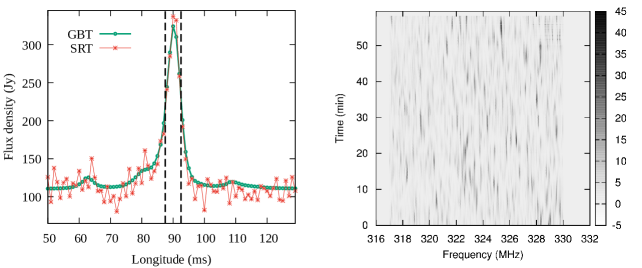
Figure 1: Left-hand panel: average profile obtained in an observing scan. The vertical dashed lines delineate the window used for calculation of the on-pulse dynamic spectra and cross-spectra. Right-hand panel: dynamic spectrum based on GBT observations for the session on November 26.

The right-hand panel of Fig. 1 shows an example of the resulting dynamic spectrum $S(\nu,t)$ calculated from the data obtained at GBT on November 26. To construct the dynamic spectrum for the whole one-hour session we filled gaps between the scans by interpolating between the last and the first spectra of consecutive scans.

The interstellar scintillation causes strong variations of the observed flux density and the dynamic spectrum may be regarded as an ensemble of bright spots on the time-frequency plane called “scintles”. The primary statistical characteristics of the ensemble are the decorrelation bandwidth, $\Delta\nu_{\text{sc}}$, and the scintillation time, $t_{\text{sc}}$, that describe the average extent of the scintles in the respective directions.

For the observations used in the present paper, $\Delta\nu_{\text{sc}}$ and $t_{\text{sc}}$ were evaluated by Gwinn et al. (2016). From the analysis of the two-dimensional cross-correlation between the dynamic spectra for the LCP and RCP (left-hand and right-hand circular polarization) channels of GBT they obtained values of $\Delta\nu_{\text{sc}}\approx 15$ kHz and $t_{\text{sc}}\approx 114$ s.

3.2 Phase variations in cross-spectra

Our further analysis is based on the cross-spectra produced at the previous stage of data processing. To increase the signal-to-noise ratio, we averaged the on-pulse cross-spectra over ten consecutive pulsar periods, that is over $t_{\text{obs}}\approx 7.14$ s. In the course of averaging, we took into account only pulses that satisfy the condition $F_{\text{on}}\geq\left<F_{\text{off}}\right>+6\sigma_{\text{off}}$. Here $F_{\text{on}}$ is the flux density in the on-pulse window, $\left<F_{\text{off}}\right>$ and $\sigma_{\text{off}}$ are the mean and standard deviation of the off-pulse flux density. In rare cases where none of the pulses falling into the range of averaging meets the condition we assume that the cross-spectrum is equal to the previous one.

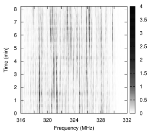
Figure 2: Time-averaged correlated flux density on the baseline SRT-GBT during a scan on November 26 in RCP channel. The averaging interval is $\approx 7.14$ s, correlated flux density is in correlator units.

Fig. 2 shows an example of the averaged cross-spectrum. Its general structure originating from the ISS closely resembles the structure in the dynamic spectrum discussed in the previous subsection. Since the averaging time, $t_{\text{obs}}$, obeys the condition $t_{\text{obs}}\ll t_{\text{sc}}$, each scintle contains, on average, $t_{\text{sc}}/t_{\text{obs}}\gg 1$ visibility measurements at different points in time, which make it possible to study the temporal variability of the complex cross-spectrum phase within individual scintles. As discussed in Section 4 below, the comparison between phase variations within different scintles permits to disentangle the ionospheric contribution to the phase shift from the effects of ISS.

The scintles used in our analysis were constructed as follows. To increase the SNR we averaged the complex cross-spectra produced by the correlator over eight channels, thus reducing the frequency resolution to 31.25 kHz (about $2\times\Delta\nu_{\text{sc}}$).

The pixels of the averaged cross-spectra that exceed in visibility magnitude the threshold of $3.5\sigma^{\text{cs}}_{\text{off}}$ are considered “bright” and form a constituent part of a scintle. Here, $\sigma^{\text{cs}}_{\text{off}}$ is the rms amplitude of the cross-spectrum measured in the off-pulse window. The pixels with the visibility magnitude below the threshold are considered ”dim” and the values of their phases are not used in further analysis. The left-hand panel of Fig. 3 illustrates the results of the application of the algorithm described above to the scan started on 2012 November 26 at 21:00 UTC.

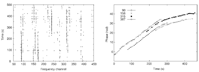
Figure 3: Left-hand panel: schematic presentation of the pixels selected for tracing the cross-spectrum phase variability for the scan started on 2012 November 26 at 21:00 UTC. The plus symbols represent bright pixels that constitute the selected scintles. Right-hand panel: phase variations for the selected scintles. The numbers in the legend specify the numbers of corresponding frequency channels in the left panel. The nearly parallel signature of the changes of phase for all scintles is interpreted as being due to the ionosphere. The offsets between the phases of the scintles may be due to characteristics of ISS.

The pixels are then grouped into scintles in such a way that (a) all pixels of a scintle reside in the same averaged frequency channel and cover a contiguous time interval, (b) first and last pixels of a scintle, as well as the majority, but not necessarily all, of intermediate pixels are bright, and (c) the time interval between two adjacent bright pixels located in the same scintle does not exceed $t_{\text{sc}}/2$.

The right-hand panel of Fig. 3 illustrates the phase as a function of time for the four strongest scintles. The initial phase of $i$-th scintle is defined only within an ambiguity of $2n_{i}\pi$, where $n_{i}$ is an arbitrary integer, and therefore only comparison of the slopes of the curves in the plot is meaningful. In creating the plot, the values $n_{i}$ were chosen in such a way as to facilitate such a comparison. The apparent offsets between the phase curves for the different scintles could be due to characteristics of the ISM but a more detailed analysis is not possible because of the $2\pi$ ambiguities and the relatively short observation times.

The phase variations for the four scintles, and in fact for all other inspected scintles, are well approximated by a piecewise linear function with the slope brake at $\approx 300$ s. For all the scintles the rate of change of the phase is nearly the same during the whole duration of the scan. The same analysis was performed for other scans and in all cases phase differences $\phi_{i}(t)-\phi_{j}(t)$ for any pair $i,\,j$ of scintles indices were constant over time within an accuracy of our measurements.

The disadvantage of this method is that removing $2\pi$ ambiguities becomes non-unique for long intervals between consecutive bright pixels. Because of the inter-scan gaps, this difficulty inevitably arises in trying to study the variability on the time-scales exceeding the duration of the scan.

To investigate the phase behaviour over longer times, we used a different approach that relies only on the instant phase shift rate, $\phi^{\,\prime}=\text{d}\phi/\text{d}t$, which we approximate by the phase difference between bright pixels separated in time by one $\approx 7.14$ s long averaging interval. This approach permits us to analyze the data without having to correct for the $2\pi$ phase ambiguities.

The left-hand panel of Fig. 4 shows the phase shift rate as a function of time during the session on 2012 November 26.

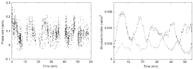
Figure 4: Left-hand panel: phase shift rate variation with time for all scintles in the one-hour session on November 26. Right-hand panel: structure functions for the phase shift rate on November 26 (solid line) and on November 29 (dashed line).

As is evident from the left-hand panel of the figure, the average value of phase shift rate, $\langle\phi^{\,\prime}\rangle$, over, say, 60 min is clearly larger than zero, meaning that $\phi$ gradially increases during the observations.

Another feature easily seen on the plot is a quasi-periodic oscillation of $\phi^{\,\prime}$ around its average value, $\langle\phi^{\,\prime}\rangle$. Our analysis of the oscillations is based on the temporal structure function of phase shift rate, $D(\tau)$, defined as

$$D(\tau)=\left\langle\left[\phi^{\,\prime}(t+\tau)-\phi^{\,\prime}(t)\right]^{2}\right\rangle\,.$$ (2)

Here $\left\langle\right\rangle$ denotes averaging over the time interval $[t_{\text{beg}},t_{\text{end}}-\tau]$ and over all selected scintles, where $t_{\text{beg}}$ and $t_{\text{end}}$ are the moments of the beginning and end of the session, respectively. If we assume that slow gradual changes in $\phi$ can be approximated by a linear dependence on $t$, then $D(\tau)$ is completely determined by the oscillatory component of $\phi^{\,\prime}(t)$.

To establish the relationship between the amplitudes of oscillation of $\phi^{\,\prime}(t)$ and $D(\tau)$, which we denote as $A_{\phi}$ and $A_{\text{D}}$, respectively, we consider the simple model where $\phi^{\,\prime}_{m}(t)=A_{\phi}\cos(2\pi t/T)+\epsilon(t)$, and where it is assumed that measurement errors $\epsilon(t)$ are normally distributed random values with variance independent of $t$, and $\left<\epsilon(t)\epsilon(t^{\prime})\right>=0$ for $t\neq t^{\prime}$. Straightforward calculation of the structure function for the model, $D_{\text{m}}(\tau)$, yields $D_{\text{m}}(\tau)=A_{\text{D}}(1-\cos(2\pi\tau/T))+\langle\epsilon^{2}\rangle$ where $A_{\text{D}}=A_{\phi}^{2}$.

The right-hand panel of Fig. 4 shows the structure functions for both observing sessions. Approximating the data by the simple model described above we may estimate the characteristic period, $T_{\phi}$, and the amplitude, $A_{\phi}$, of the observed phase shift rate variations to be: $T_{\phi}\approx 12$ min, $A_{\phi}\approx 0.030$ rad/s for the November 26 observing session, and $T_{\phi}\approx 10$ min, $A_{\phi}\approx 0.015$ rad/s for the November 29 observing session.

4 Origin of the observed phase variations

Two principal effects that may cause temporal variability in cross-spectrum phase – interstellar scintillations and changes in parameters of the ionosphere – are distinguishable from one another through their dependence on observation frequency.

In space-ground interferometry, the principal parameter of the ionosphere that determines its influence on the observed visibility phase is the total electron content (TEC) at the location of the ground telescope. TEC is defined as

$$C_{\text{e}}=\int_{0}^{\infty}n_{\text{e}}(h)\,dh\,,$$ (3)

where $n_{\text{e}}(h)$ is the electron density at height $h$. Since our observing frequency, $\nu$, satisfies the condition $\nu\gg\nu_{\text{p}}$, where $\nu_{\text{p}}\loa 12$ MHz is the typical plasma frequency of the ionosphere, we can use the high-frequency approximation for the plasma refractive index. The ionosperically induced phase shift, $\Delta\phi$, is then given by

$$\Delta\phi=-8.45\frac{C_{\text{e}}}{10^{16}\,{\text{m}}^{-2}}\frac{1\,\text{GHz}}{\nu}\sec z\,,$$ (4)

where $z$ is the zenith angle of the observed object (Mevius et al., 2016; Thompson et al., 2017).

The scintles used in Section 3.2 for the analysis of phase variability cover the frequency range, $\Delta\nu_{\text{sp}}$, of about 12 MHz (see Fig. 2). Ionospheric phase variations in all the scintles are governed by changes in the single parameter, $C_{\text{e}}$. Expected relative difference in the magnitude of the slopes of dependence $\phi(t)$ for any two scintles is less than $\Delta\nu_{\text{sp}}/\nu\approx 0.04$ for the whole observing band and less then 0.03 for the brightest scintles presented in right-hand panel of Fig. 3. Consequently, the values $\phi_{i}(t)-\phi_{j}(t)$, where $\phi_{i}(t)$ is the ionospheric phase shift measured at the $i$-th scintle, remain nearly constant in the course of a scan.

In contrast, phase variations due to ISS in widely ($\Delta\nu>\Delta\nu_{\text{sc}}$) separated scintles are expected to be weakly correlated, since different scintles originate from the interference of the rays passing through different regions of the scattering interstellar plasma.

If we suppose that each cross-spectrum scintle originates from an element of the scattering disk substructure, then ISS contribution to temporal variations of observed phase differences $\phi_{i}(t)-\phi_{j}(t)$ reflects relative motion of the corresponding substructure elements.

As it is illustrated in Fig. 3, our observations do not show any noticeable deviations from the synchronous phase changes in different scintles, which is compatible with the assumption that the observed temporal variations are dominated by the ionospheric contribution, and ISS effects are below the sensitivity of our method.

To explain the slowly varying component of the observed temporal variability pattern, we note that the observations were made in the time range 21:00 to 22:00 UTC, during the last hour before the sunset at GBT. The telescope tracked the source in the azimuth range 35–40° and in the range of elevation angles 20–27°. The nearly linear trend in phase can be attributed to diurnal variations in TEC in the ionosphere above GBT and the decrease in $\sec z$ of the ascending source.

Before proceeding to the interpretation of the quasi-periodic phase variations, we estimate the amplitude of changes in TEC above the GBT that correspond to the amplitude, $A_{\phi}$, and time-scale, $T_{\phi}$, of the observed oscillations of $\phi^{\,\prime}$. With the amplitude of phase variations, $\Delta\phi$, approximated by $\Delta\phi\approx A_{\phi}T_{\phi}/\pi$ and the values for $A_{\phi}$ and $T_{\phi}$ from Section 3.2, the amplitudes of TEC oscillations are $\approx 0.1\times 10^{16}$ and $\approx 0.05\times 10^{16}\,\text{m}^{-2}$ on November 26 and 29, respectively.

The observed amplitudes of TEC oscillations, time-scales of quasi-periodicity, and low amplitude attenuation rates indicate that the oscillations originate probably from medium-scale travelling ionospheric disturbances (TID). Ionospheric disturbances were studied in many publications by various methods. Applications of VLBI to the problem are described, e.g., by Zhi-Han & Yong (1993), Hobiger et al. (2006), Heinkelmann et al. (2009), Helmboldt (2014)). A review of important aspects related to probing the ionosphere with RadioAstron was given by Zhuravlev et al. (2020). It is generally accepted that TIDs are a manifestation of atmospheric gravity waves (AGW) in the ionosphere (Hocke & Schlegel, 1996). A short review of TIDs is provided by Crowley & Azeem (2018). According to them, there are several geophysical phenomena – ocean waves, tsunamis, explosions, weather fronts, and thunderstorms – that might excite medium-scale AGWs, and consequently TIDs.

The typical time-scale of oscillations caused by medium-scale TIDs is 10–30 minutes. Azeem et al. (2017) reported the observations of TIDs excited by earthquakes and subsequent tsunami-launched AGWs using GPS total electron content (TEC) data. They found a maximum amplitude of variations in TEC of $\approx 1.1\times 10^{16}\,{\text{m}}^{-2}$, and a decay time of about four hours. Thus, the phase oscillations that we observed closely resemble the variations induced by medium-scale TIDs.

5 Conclusion

We present an analysis of two-element interferometry data in the frequency range 316-332 MHz with the Earth–space baseline GBT-SRT for PSR B0329+54. Analyzing interferometer phase variations in scintles produced by the interstellar medium, we show that ionospheric effects on the phase can be clearly identified and quantified.

Cross-spectrum phases were monitored over time for several scintles. Variations that occurred synchronously in the scintles over the whole frequency range of the bandpass are attributed to variations of the ionosphere. Phase changes due to the effects of interstellar scintillation are expected to be uncorrelated for scintles widely separated in frequency.

The time dependence of the phase was calculated for individual scintles. Intercomparison of cross-spectrum phases measured for multiple scintles permits to identify the origin of phase variations. The variations arising from the ionosphere occur synchronously in the scintles over the whole frequency range, while phase changes due to effects of interstellar scattering are expected to be uncorrelated for the scintles widely separated in frequency.

We found that the observed phase variations are nearly frequency independent, which means that they are dominated by the ionospheric contribution. Phase dependence on time may be expressed as a sum of a slowly varying quasi-linear component and quasi-periodic oscillations. The slowly varying component is naturally explained by the diurnal variations of electronic density in the ionosphere and the changes in the zenith distance of the pulsar as seen by the GBT.

The oscillatory component corresponds to quasi-periodic variations in the TEC in the ionosphere above the GBT with amplitudes of (0.05–0.1)$\times 10^{16}\,\text{m}^{-3}$, time-scales of 10–12 min, and decay times exceeding one hour. The TEC varions of this type are likely caused by the medium-scale travelling ionospheric disturbances.

Interstellar scattering limits the coherent integration time, $t_{\text{obs}}$, for pulsar VLBI studies by the value of scintillation time, $t_{\text{sc}}$, which is typically from several seconds to several minutes (Goodman & Narayan, 1989; Gwinn et al., 1998). These constraints do not apply to VLBI studies of extragalactic radio sources because their intrinsic angular sizes are large enough to quench diffraction scintillations in frequency and time (Walker, 1998). Therefore, only ionospheric and atmospheric effects would limit the coherent integration time for these sources. In particular, the observed medium-scale Travelling Ionospheric Disturbances would pose the constraint $t_{\text{obs}}\ll T_{\phi}$ on the duration of low-frequency observations.

Data availability

The data underlying this article are available in the RadioAstron data archive at ftp://ftp.radioastron.ru/raes10/, and can be accessed with observation codes raes10a and raes10d

References

- Azeem et al. (2017) Azeem I., Vadas S. L., Crowley G., Makela J. J., 2017, Journal of Geophysical Research (Space Physics), 122, 3430
- Brisken et al. (2002) Brisken W. F., Benson J. M., Goss W. M., Thorsett S. E., 2002, ApJ, 571, 906
- Crowley & Azeem (2018) Crowley G., Azeem I., 2018, in Buzulukova N., ed., , Extreme Events in Geospace. Elsevier, pp 555 – 586, doi:https://doi.org/10.1016/B978-0-12-812700-1.00023-6
- Goodman & Narayan (1989) Goodman J., Narayan R., 1989, MNRAS, 238, 995
- Greisen (2016) Greisen E. W., 2016, AIPS Memo 114, The FITS Interferometry Data Interchange Convention — Revised. NRAO, Socorro, NM
- Gwinn et al. (1998) Gwinn C. R., Britton M. C., Reynolds J. E., Jauncey D. L., King E. A., McCulloch P. M., Lovell J. E. J., Preston R. A., 1998, ApJ, 505, 928
- Gwinn et al. (2016) Gwinn C. R., et al., 2016, ApJ, 822, 96
- Heinkelmann et al. (2009) Heinkelmann R., Hobiger T., Schmidt M., 2009, in EGU General Assembly Conference Abstracts. EGU General Assembly Conference Abstracts. p. 5715
- Helmboldt (2014) Helmboldt J., 2014, in AGU Fall Meeting Abstracts. pp SA11B–3940
- Hobbs et al. (2006) Hobbs G., Edwards R., Manchester R., 2006, Chinese Journal of Astronomy and Astrophysics Supplement, 6, 189
- Hobiger et al. (2006) Hobiger T., Kondo T., Schuh H., 2006, Radio Science, 41, RS1006
- Hocke & Schlegel (1996) Hocke K., Schlegel K., 1996, Annales Geophysicae, 14, 917
- Kardashev et al. (2013) Kardashev N. S., et al., 2013, Astronomy Reports, 57, 153
- Likhachev et al. (2017) Likhachev S. F., Kostenko V. I., Girin I. A., Andrianov A. S., Rudnitskiy A. G., Zharov V. E., 2017, Journal of Astronomical Instrumentation, 6, 1750004
- Mevius et al. (2016) Mevius M., et al., 2016, Radio Science, 51, 927
- Pence (1999) Pence W., 1999, in Mehringer D. M., Plante R. L., Roberts D. A., eds, Astronomical Society of the Pacific Conference Series Vol. 172, Astronomical Data Analysis Software and Systems VIII. p. 487
- Popov et al. (2017) Popov M. V., et al., 2017, MNRAS, 465, 978
- Popov et al. (2020) Popov M. V., Bartel N., Burgin M. S., Gwinn C. R., Smirnova T. V., Soglasnov V. A., 2020, ApJ, 888, 57
- Ros et al. (2000) Ros E., Marcaide J. M., Guirado J. C., Sardón E., Shapiro I. I., 2000, A&A, 356, 357
- Thompson et al. (2017) Thompson A. R., Moran J. M., Swenson George W. J., 2017, Interferometry and Synthesis in Radio Astronomy, 3rd Edition. Springer, Cham, doi:10.1007/978-3-319-44431-4
- Walker (1998) Walker M. A., 1998, MNRAS, 294, 307
- Zhi-Han & Yong (1993) Zhi-Han Q., Yong Z., 1993, in Mueller I. I., Kolaczek B., eds, Vol. 156, Developments in Astrometry and their Impact on Astrophysics and Geodynamics. p. 207
- Zhuravlev et al. (2020) Zhuravlev V. I., Yermolaev Y. I., Andrianov A. S., 2020, MNRAS, 491, 5843