On a sinc-type MBE model

Abstract.

We introduce a new sinc-type molecular beam epitaxy model which is derived from a cosine-type energy functional. The landscape of the new functional is remarkably similar to the classical MBE model with double well potential but has the additional advantage that all its derivatives are uniformly bounded. We consider first order IMEX and second order BDF2 discretization schemes. For both cases we quantify explicit time step constraints for the energy dissipation which is in good accord with the practical numerical simulations. Furthermore we introduce a new theoretical framework and prove unconditional uniform energy boundedness with no size restrictions on the time step. This is the first unconditional (i.e. independent of the time step size) result for semi-implicit methods applied to the phase field models without introducing any artificial stabilization terms or fictitious variables.

1. Introduction

In this work we consider the following molecular beam epitaxy (MBE) model posed on the two dimensional periodic torus $\Omega=\mathbb{T}^{2}=[-\pi,\pi]^{2}$:

$$\partial_{t}h=-\eta^{2}\Delta^{2}h-\nabla\cdot(\mathrm{sinc}(|\nabla h|)\nabla h),\qquad(t,x)\in(0,\infty)\times\Omega,$$ (1.1)

where $\mathrm{sinc}(t)=\sin t/t$ is the usual $\mathrm{sinc}$-function and

$$|\nabla h|=\sqrt{(\partial_{x_{1}}h)^{2}+(\partial_{x_{2}}h)^{2}}.$$ (1.2)

The function $h=h(t,x)$ represents a scaled height function of thin film and $\eta^{2}$ is a positive constant. Note that since the power series of $\mathrm{sinc}(t)$ consists only even powers of $t$, the term $\mathrm{sinc}(|\nabla h|)$ is a bounded smooth function in $|\nabla h|^{2}=\nabla h\cdot\nabla h$. Furthermore

$$\sup_{z\in\mathbb{R}^{2}}|\partial_{z_{1}}^{k_{1}}\partial_{z_{2}}^{k_{2}}(\mathrm{sinc}(|z|)z)|<\infty,\qquad\forall\,k_{1},k_{2}\geq 0.$$ (1.3)

Thanks to this simple observation it is a breeze to build a wellposedness theory for (1.1). The equation (1.1) can be regarded as a $L^{2}$ gradient flow of the energy functional

$$\mathcal{E}(h)=\int_{\Omega}\Bigl{(}\frac{1}{2}\eta^{2}|\Delta h|^{2}+\cos(|\nabla h|)\Bigr{)}dx.$$ (1.4)

Consequently for smooth solutions, we have the energy identity

$$\mathcal{E}(h(t_{2}))+\int_{t_{1}}^{t_{2}}\|\partial_{t}h\|_{2}^{2}dt=\mathcal{E}(h(t_{1})),\qquad\forall\,0\leq t_{1}<t_{2}<\infty.$$ (1.5)

In particular we have

$$\mathcal{E}(h(t))\leq\mathcal{E}(h(0)),\qquad\forall\,t>0.$$ (1.6)

By using this fundamental monotonicity law in conjunction with the smoothness and boundedness of the nonlinearity, one can obtain global wellposedness and regularity for (1.1) with $H^{2}$ (or rougher) initial data. Note that for $|z|\ll 1$, we have

$$\cos z=\frac{1}{24}(z^{2}-6)^{2}-\frac{1}{2}+O(|z|^{6}).$$ (1.7)

Thus up to a harmless additive constant, the energy functional (1.4) is similar to the standard double well-potential (see Section 2 (2.8)–(2.9)), namely

$$\mathcal{E}_{\mathrm{st}}(h) =\int_{\Omega}\Bigl{(}\frac{1}{2}\eta^{2}|\Delta h|^{2}+\frac{1}{24}(|\nabla h|^{2}-6)^{2}\Bigr{)}dx.$$ (1.8)

In the MBE literature, it is well-known that the energy functional (1.8) leads to the thin film model with slope selection (cf. [16] and [37]). However a fundamental difficulty with the analysis and simulation of the dynamical equation corresponding to (1.8) is the lack of good Lipschitz bounds on the nonlinearity (see [21, 19]). In stark contrast our model (1.1) and its cousins has a “built-in” control of the Lipschitz norms which renders the analysis and simulation much more appealing. Moreover these new models satisfy Onsager’s reciprocity relations and capture much the same physics as prototypical MBE models. To discuss these connections and put things into perspective we review below some prior arts and related analysis.

Molecular beam epitaxy (MBE) is a process for growing thin, epitaxial films of a wide variety of materials, ranging from oxides to semiconductors and metals. It is first used in the epitaxial growth of compound semiconductor films by a process involving the reaction of one or more thermal molecular beams with a crystalline surface under ultra-high vaccum conditions. These arriving constituent atoms form a crystalline layer in registry with the substrate, i.e., an epitaxial film. To understand the mechanism of this physical process, several different PDE models have been proposed for investigating the morphological instability and interfacial dynamics at various temporal and spatial scales [15, 36]. In a fixed Cartesian coordinate system, one can denote $h_{\mathrm{real}}$ as the actual height of the film at time $t$, and traces the evolution of $h(t,x)=h_{\mathrm{real}}-Ft$ where $F$ stands for the deposition flux. In yet other words the film surface at time $t$ is represented by $x_{3}=h(t,x_{1},x_{2})$ in a co-moving frame. By using conservation of mass, we have

$$h_{t}=-\Omega_{a}\nabla\cdot J,$$ (1.9)

where $\Omega_{a}$ is the atomic volume and $J$ is the surface current. On a purely phenomenological basis and considering only isotropic growth, we may represent the surface current as a series (cf. [27, 38, 39] )

$$J=A_{1}\nabla h+A_{2}\nabla(\Delta h)+A_{3}|\nabla h|^{2}\nabla h+A_{4}\nabla|\nabla h|^{2}+\cdots,$$ (1.10)

In (1.10) one typically only retains terms vanishing no faster than $L^{-4}$. Plugging this into (1.9), we arrive at

$$\partial_{t}h=~{} -\Omega_{a}\Bigl{(}A_{1}\Delta h+A_{2}\Delta^{2}h+A_{3}\nabla\cdot(|\nabla h|^{2}\nabla h)+A_{4}\Delta(|\nabla h|^{2})\Bigr{)}.$$ (1.11)

The physical meaning of each term is as follows:

• $A_{1}\Delta h$: diffusion by particle exchange between surface and the vapor (Mullins [24]);

• $A_{2}\Delta^{2}h$: capillarity-driven surface diffusion (Mullins [24], Herring [10]);

• $A_{3}\nabla\cdot(|\nabla h|^{2}\nabla h)$: consistent with an atomistic model by Das Sarma-Ghaisas [6];

• $A_{4}\Delta(|\nabla h|^{2})$: Lai-Das Sarma [17] used it to describe the model where an atom moves to a neighboring kink site and breaks the bond to find another kink with smaller step height.

As it was well explained in [17], each of these terms can be viewed as a building block to form composite structures such as peaks, valeys and so on (see figure 1 for the 1D case). In [27], the term $A_{4}\Delta(|\nabla h|^{2})$ was dropped in view of Onsager’s reciprocity relations ([25, 26, 28]). By a relabelling of the constants, this leads to the standard model

$$\partial_{t}h=-D\Delta^{2}h+v\nabla\cdot((k^{-2}|\nabla h|^{2}-1)\nabla h).$$ (1.12)

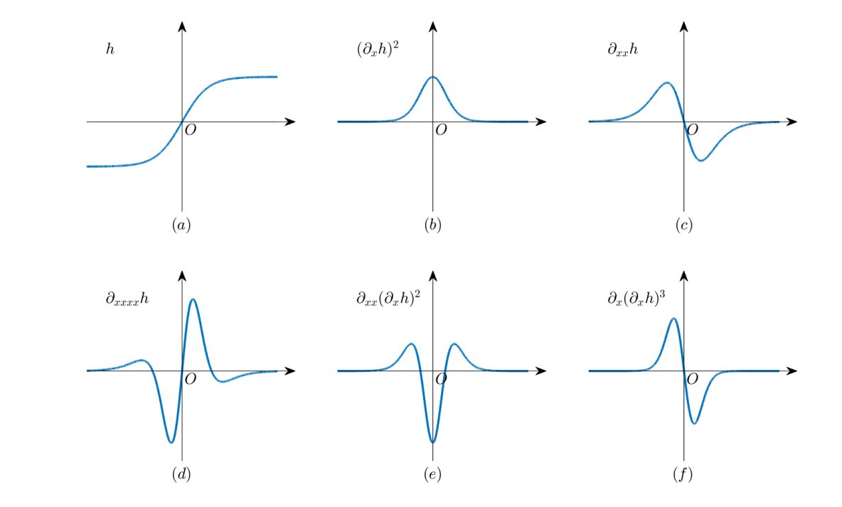
Figure 1. Schematic diagram of $h=\tanh(x)$ and its derivatives.

In Section 2, we shall show that our model (1.1) corresponds to the expansion (1.10) by carefully incorporating higher order terms which satisfy Onsager’s reciprocity relations. In the regime $|\nabla h|\ll 1$ our model coincides with the standard MBE model with slope selection. On the other hand, it is vastly different from the MBE model without slope selection (cf. [16])

$$\partial_{t}h=-\eta^{2}\Delta^{2}h-\nabla\cdot(\frac{\nabla h}{1+|\nabla h|^{2}}),$$ (1.13)

since its energy functional $\mathcal{E}(h)=\int_{\Omega}(\frac{\eta^{2}}{2}|\Delta h|^{2}-\frac{1}{2}\ln(|1+|\nabla h|^{2}))dx$ behaves badly and leads to mound-like structures. Note that a nice feature of (1.13) is that its nonlinearity has bounded derivatives of all orders. However its energy landscape is different from the standard MBE model with slope selection. Our model can be regarded as a variant of the standard MBE model with slope selection and with tamed nonlinearity (in terms of Lipschitz control). In future works we plan to carry out an in-depth comparative study of our new model with existing standard models.

The main contribution of this work is as follows.

1. We introduce a new sinc-type molecular beam epitaxy model which is derived from a cosine-type energy functional. The landscape of the new functional is remarkably similar to the classical MBE model with double well potential but has the additional advantage that all its derivatives are uniformly bounded. Furthermore it captures the same physics as the classical MBE model with slope selection. It is possible to generalize our approach to a more systematic construction of “benign” free energies whilst keeping the same physics.

2. We consider first order IMEX and second order BDF2 discretization schemes. For both cases we quantify explicit time step constraints for the energy dissipation which is in good accord with the practical numerical simulations.

3. We introduce a new theoretical framework and prove unconditional uniform energy boundedness with no size restrictions on the time step. This is the first unconditional (i.e. independent of the time step size) result for semi-implicit methods applied to the phase field models without introducing any artificial stabilization terms or fictitious variables.

The rest of this paper is organized as follows. In Section 2 we give a more detailed derivation of the model and explain its connection with earlier models. In Section 3 and 4 we consider first order IMEX discretization and prove the energy stability bounds. In Section 5 and 6 we carry out the analysis for BDF2 methods. Section 7 collects several numerical simulations with side by side comparisons with existing MBE models. In the final section we give concluding remarks.

2. Derivation of the model

To allow some generality, we start with the energy functional

$$\mathcal{E}=\int_{\Omega}\Bigl{(}\frac{1}{2}\eta^{2}|\Delta h|^{2}+\beta_{1}\cos(\beta|\nabla h|)\Bigr{)}dx,$$ (2.1)

where $\beta_{1}$, $\beta$ are constants.

Denote

$$g_{1}(t)=\sum_{k=0}^{\infty}\frac{(-1)^{k}t^{k}}{(2k)!}=1+\sum_{k=1}^{\infty}\frac{(-1)^{k}t^{k}}{(2k)!}.$$ (2.2)

Note that

$$g_{1}^{\prime}(t)=\frac{1}{2}\sum_{k=1}^{\infty}\frac{(-1)^{k}}{(2k-1)!}t^{k-1},$$

$$g_{1}^{\prime}(s^{2})=-\frac{1}{2}s^{-1}\sin s.$$ (2.3)

Here the identity (2.3) also holds at $s=0$ provided we identify $\frac{\sin s}{s}\Bigr{|}_{s=0}=1$.

Clearly

$$\mathcal{F}=\int_{\Omega}\cos(\beta|\nabla h|)dx=\int_{\Omega}g_{1}(\beta^{2}|\nabla h|^{2})dx,$$ (2.4)

$$\frac{\delta\mathcal{F}}{\delta h}\Bigr{|}_{L^{2}}=-2\beta^{2}\nabla\cdot(g_{1}^{\prime}(\beta^{2}|\nabla h|^{2})\nabla h),$$ (2.5)

where $\frac{\delta\mathcal{F}}{\delta h}\Bigr{|}_{L^{2}}$ denotes the variational derivative of the functional $\mathcal{F}$ in $L^{2}$. By (2.3), it follows that

$$\frac{\delta\mathcal{F}}{\delta h}\Bigr{|}_{L^{2}}=\beta^{2}\nabla\cdot(\frac{\sin(\beta|\nabla h|)}{\beta|\nabla h|}\nabla h).$$ (2.6)

Thus

$$\frac{\delta\mathcal{E}}{\delta h}\Bigr{|}_{L^{2}}=\eta^{2}\Delta^{2}h+\beta^{2}\beta_{1}\nabla\cdot(\mathrm{sinc}(\beta|\nabla h|)\nabla h).$$ (2.7)

Note that for $|\nabla h|\ll 1$, we have

$$\mathrm{sinc}(\beta|\nabla h|)=1-\frac{1}{6}\beta^{2}|\nabla h|^{2}+O(|\nabla h|^{4}).$$ (2.8)

Taking $\beta_{1}=1/6$ and $\beta=\sqrt{6}$, we then recover the usual MBE model with slope selection:

$$\partial_{t}h=-\frac{\delta\mathcal{E}}{\delta h}\Bigr{|}_{L^{2}}=-\eta^{2}\Delta^{2}h-\nabla\cdot((1-|\nabla h|^{2})\nabla h).$$ (2.9)

We now explain the connection with the general model mentioned in the introduction especially concerning the expansion (1.10).

2.1. Connection with the general model.

Firstly, we start with the expansion

$$J={} A_{1}\nabla h+A_{2}\nabla(\Delta h)+A_{3}|\nabla h|^{2}\nabla h+A_{4}\nabla|\nabla h|^{2}+\sum_{i=1}^{\infty}A_{4+i}|\nabla h|^{2+2i}\nabla h.$$ (2.10)

Substituting (2.10) into (1.10) we get

$$h_{t}={} -\Omega_{a}\Big{[}A_{1}\Delta h+A_{2}\Delta^{2}h+A_{3}\nabla\cdot(|\nabla h|^{2}\nabla h)+A_{4}\Delta|\nabla h|^{2}$$ (2.11)

$$+\sum_{i=1}^{\infty}A_{4+i}\nabla\cdot(|\nabla h|^{2+2i}\nabla h|)\Big{]}.$$

Enforcing Onsager’s reciprocity relations (see [25, 26, 28]), we can drop the $A_{4}$ term. Thus

$$\partial_{t}h=-c\nabla\cdot(\nabla h(1-\sum_{i=1}^{\infty}B_{i}|\nabla h|^{2i}))-D\Delta^{2}h,$$ (2.12)

where $c=\Omega_{a}A_{1}$, $B_{1}=-\frac{A_{3}}{A_{1}}$, $B_{i}=-\frac{A_{3+i}}{A_{1}}$ for $i\geq 2$ and $D=\Omega_{a}A_{2}$. When the coefficients $B_{i}$ satisfy

$$B_{i}=\frac{(-1)^{i-1}}{(2i+1)!}\quad\mbox{for}\quad i\geq 1,$$ (2.13)

we obtain

$$\partial_{t}h=-D\Delta^{2}h-c\nabla\cdot\left(\frac{\sin(|\nabla h|)}{|\nabla h|}\nabla h\right).$$ (2.14)

3. Energy decay of first order IMEX

We consider the following first order implicit-explicit (IMEX) scheme:

$$\frac{h^{n+1}-h^{n}}{\tau}=-\eta^{2}\Delta^{2}h^{n+1}+\nabla\cdot(g(\nabla h^{n})),$$ (3.1)

where

$$g(z)=-\frac{\sin(|z|)}{|z|}z,\quad z\in\mathbb{R}^{2}.$$ (3.2)

Lemma 3.1.

Let $G(z)=\cos|z|=\cos\sqrt{z_{1}^{2}+z_{2}^{2}}$ for $z\in\mathbb{R}^{2}$. Then

$$\sum_{i,j=1}^{2}x_{i}x_{j}\partial_{z_{i}}\partial_{z_{j}}G(z)\leq|x|^{2},\qquad\forall\,x,z\in\mathbb{R}^{2}.$$ (3.3)

Proof.

With no loss we assume $z\neq 0$. By a simple computation we have

$$\partial_{z_{i}}\partial_{z_{j}}G=-\left(\cos|z|-\frac{\sin|z|}{|z|}\right)\frac{z_{i}z_{j}}{|z|^{2}}-\frac{\sin|z|}{|z|}\delta_{ij}.$$ (3.4)

Thus

$$\sum_{i,j=1}^{2}x_{i}x_{j}\partial_{z_{i}}\partial_{z_{j}}G(z) =\left(-\cos|z|+\frac{\sin|z|}{|z|}\right)\frac{|x\cdot z|^{2}}{|z|^{2}}-\frac{\sin|z|}{|z|}|x|^{2}$$

$$=(-\cos|z|)\frac{|x\cdot z|^{2}}{|z|^{2}}-\frac{\sin|z|}{|z|}|x\cdot z^{\perp}|^{2},$$ (3.5)

where $z^{\perp}$ is a unit vector orthogonal to $z$. The desired result then easily follows. ∎

For simplicity of notation, we denote

$$E_{n}=\int_{\Omega}\Bigl{(}\frac{\eta^{2}}{2}|\Delta h^{n}|^{2}+\cos|\nabla h^{n}|\Bigr{)}dx.$$ (3.6)

Theorem 3.1 (Energy dissipation).

Consider the IMEX scheme (3.1) with $h^{0}\in H^{2}(\mathbb{T}^{2})$. For any $n\geq 0$,

$$E_{n+1}-E_{n}+(\sqrt{\frac{2\eta^{2}}{\tau}}-\frac{1}{2})\|\nabla(h^{n+1}-h^{n})\|_{2}^{2}\leq 0,$$ (3.7)

In particular if

$$0<\tau\leq{8\eta^{2}},$$ (3.8)

then $E_{n+1}\leq E_{n}$ for all $n\geq 0$.

Proof.

Taking the $L^{2}$-inner product with $(h^{n+1}-h^{n})$ on both sides of (3.1), we get

$$\frac{1}{\tau}\|h^{n+1}-h^{n}\|_{2}^{2}+\frac{\eta^{2}}{2}(\|\Delta h^{n+1}\|_{2}^{2}-\|\Delta h^{n}\|_{2}^{2}+\|\Delta(h^{n+1}-h^{n})\|_{2}^{2})=-(g(\nabla h^{n}),\nabla(h^{n+1}-h^{n})).$$

Denote $G(z)=\cos|z|=\cos\sqrt{z_{1}^{2}+z_{2}^{2}}$ for $z\in\mathbb{R}^{2}$. Introduce

$$H(s)=G(\nabla h^{n}+s(\nabla h^{n+1}-\nabla h^{n})).$$

By using the expansion

$$H(1)=H(0)+H^{\prime}(0)+\int_{0}^{1}H^{\prime\prime}(s)(1-s)ds,$$

we get

$$G(\nabla h^{n+1}) -G(\nabla h^{n})=g(\nabla h^{n})\cdot(\nabla h^{n+1}-\nabla h^{n})$$

$$\;+\sum_{i,j=1}^{2}\partial_{i}(h^{n+1}-h^{n})\partial_{j}(h^{n+1}-h^{n})\int_{0}^{1}(\partial_{ij}G)(\nabla h^{n}+s(\nabla h^{n+1}-\nabla h^{n}))(1-s)ds.$$

By Lemma 3.1, we obtain

$$E_{n+1}-E_{n}+\frac{1}{\tau}\|h^{n+1}-h^{n}\|_{2}^{2}+\frac{\eta^{2}}{2}\|\Delta(h^{n+1}-h^{n})\|_{2}^{2}\leq\frac{1}{2}\|\nabla(h^{n+1}-h^{n})\|_{2}^{2}.$$ (3.9)

The desired inequality now follows from this and the simple interpolation inequality

$$\|\nabla h\|_{2}\leq\|h\|_{2}^{\frac{1}{2}}\|\Delta h\|_{2}^{\frac{1}{2}}.$$ (3.10)

∎

4. Uniform boundedness of the energy for any $\tau>0$

Theorem 4.1 (Unconditional uniform energy boundedness).

Consider the scheme (3.1) with $\tau>0$ and $h^{0}\in H^{2}(\mathbb{T}^{2})$. We have

$$\sup_{n\geq 1}(\|h^{n}\|_{2}+\|\Delta h^{n}\|_{2})\leq C_{1}<\infty,$$ (4.1)

where $C_{1}>0$ depends only on $(h^{0},\eta)$. Note that $C_{1}$ is independent of $\tau$.

Proof.

We begin by noting that

$$\int_{\Omega}h^{n}dx=\int_{\Omega}h^{0}dx,\qquad\forall\,n\geq 1.$$ (4.2)

Thus with no loss we may assume $\int_{\Omega}h^{n}dx=0$ for all $n\geq 0$. This will justify the use of the Poincaré inequality in our proof below.

Taking the $L^{2}$-inner product with $h^{n+1}$ on both sides of (3.1), we obtain

$$\frac{\|h^{n+1}\|_{2}^{2}-\|h^{n}\|_{2}^{2}+\|h^{n+1}-h^{n}\|_{2}^{2}}{2\tau}+\eta^{2}\|\Delta h^{n+1}\|_{2}^{2}=-(g(\nabla h^{n}),\nabla h^{n+1}),$$ (4.3)

where $(\cdot,\cdot)$ denotes the usual $L^{2}$-inner product. Since $\|g\|_{\infty}\leq 1$, we obtain

$$-(g(\nabla h^{n}),\nabla h^{n+1})\leq\|\nabla h^{n+1}\|_{1}\leq 2\pi\|\nabla h^{n+1}\|_{2}\leq 2\pi\|\Delta h^{n+1}\|_{2}.$$ (4.4)

Therefore we obtain for all $n\geq 0$,

$$\frac{\|h^{n+1}\|_{2}^{2}-\|h^{n}\|_{2}^{2}}{2\tau}+\eta^{2}\|\Delta h^{n+1}\|_{2}^{2}\leq 2\pi\|\Delta h^{n+1}\|_{2}.$$ (4.5)

For convenience of notation, we rewrite it as

$$\frac{\|h^{n}\|_{2}^{2}-\|h^{n-1}\|_{2}^{2}}{2\tau}+\eta^{2}\|\Delta h^{n}\|_{2}^{2}\leq 2\pi\|\Delta h^{n}\|_{2},\qquad\forall\,n\geq 1.$$ (4.6)

By using (4.6), we can derive

$$\sup_{n\geq 0}\|h^{n}\|_{2}\leq C_{2},$$ (4.7)

where $C_{2}>0$ depends only on $(h^{0},\eta)$.

To show (4.7), consider the set

$$S=\{n\geq 1:\,\|\Delta h^{n}\|_{2}\leq\frac{2\pi}{\eta^{2}}\}.$$ (4.8)

Case 1: $S$ is the empty set. In this case by using (4.6), we have

$$\|h^{n}\|_{2}\leq\|h^{n-1}\|_{2},\qquad\forall\,n\geq 1.$$ (4.9)

This immediately yields (4.7).

Case 2: $S$ is the set of natural numbers. Then since all $n\geq 1$ are in the set $S$, the estimate (4.7) follows from the Poincaré inequality.

Case 3: $S$ is a proper nonempty subset of the set of natural numbers. We only need to show the uniform $L^{2}$ estimate for any $n\notin S$. Now consider any $n\notin S$. We discuss two subcases.

Subcase 3a: $S\cap\{j:\,1\leq j<n\}$ is an empty set. In yet other words, all $j<n$ are not in $S$. Then in this case by using (4.6), we have

$$\|h^{j}\|_{2}\leq\|h^{j-1}\|_{2},\qquad\forall\,1\leq j\leq n.$$ (4.10)

Thus this case is OK.

Subcase 3b: There exists some $j_{*}<n$ with $j_{*}\in S$. With no loss we assume $[j_{*}+1,n]\cap S$ is an empty set. By using the Poincaré inequality, we have

$$\|h^{j_{*}}\|_{2}\leq\frac{2\pi}{\eta^{2}}.$$ (4.11)

For all $j_{*}+1\leq j\leq n$, by using (4.6) we have

$$\|h^{j}\|_{2}\leq\|h^{j-1}\|_{2}.$$ (4.12)

Thus in this case we obtain

$$\|h^{n}\|_{2}\leq\frac{2\pi}{\eta^{2}}.$$ (4.13)

Collecting the estimates, we have proved (4.7). Now to obtain the uniform $H^{2}$-estimate, we argue as follows.

Clearly, with no loss we can assume $\tau>8\eta^{2}$ since the case $0<\tau\leq 8\eta^{2}$ is already covered by Theorem 3.1.

We rewrite (3.1) as

$$\eta^{2}\Delta^{2}h^{n+1}=-\frac{h^{n+1}-h^{n}}{\tau}+\nabla\cdot(g(\nabla h^{n})).$$ (4.14)

Since $\|g\|_{\infty}\leq 1$, we have

$$\|(-\Delta)^{-1}\nabla\cdot(g(\nabla h^{n}))\|_{2}\leq O(1),$$ (4.15)

where $O(1)$ denotes a constant depending only on $(h^{0},\eta)$. Clearly by using (4.7), (4.15) and the fact that $\tau\gtrsim 1$, we obtain

$$\eta^{2}\|\Delta h^{n+1}\|_{2}\leq O(1),\qquad\forall\,n\geq 0.$$ (4.16)

∎

Remark 4.1.

Our results can be generalized to more general nonlinearities with bounded derivatives. For example, consider the following Cahn-Hilliard type equation

$$\partial_{t}u=-\Delta(\eta^{2}\Delta u-f(u)),\qquad(t,x)\in(0,\infty)\times\mathbb{T}^{2},$$ (4.17)

where $u$ is a scalar-valued function. Assume $f(z)=F^{\prime}(z)$ and

$$\|F\|_{\infty}\leq N_{0}<\infty,\;\|f\|_{\infty}\leq N_{1}<\infty,\;\sup_{z\in\mathbb{R}}f^{\prime}(z)\leq N_{2}<\infty,$$ (4.18)

where $N_{i}>0$, $i=0,1,2$ are constants. Denote

$$\mathcal{E}(u)=\int_{\mathbb{T}^{2}}\left(\frac{1}{2}\eta^{2}\|\nabla u\|_{2}^{2}+F(u)\right)dx.$$ (4.19)

Consider the first order IMEX discretization of the form:

$$\frac{u^{n}-u^{n-1}}{\tau}=-\Delta(\eta^{2}\Delta u^{n}-f(u^{n-1})),\quad n\geq 1.$$ (4.20)

Assume $u^{0}\in H^{1}(\mathbb{T}^{2})$ with mean zero. Then

$$\frac{1}{\tau}\||\nabla|^{-1}(u^{n}-u^{n-1})\|_{2}^{2}+\frac{\eta^{2}}{2}\|\nabla(u^{n}-u^{n-1})\|_{2}^{2}+\mathcal{E}(u^{n})-\mathcal{E}(u^{n-1})\leq\frac{1}{2}N_{2}\|u^{n}-u^{n-1}\|_{2}^{2},\quad\forall\,n\geq 1.$$ (4.21)

It follows that if $0<\tau\leq\frac{8\eta^{2}}{N_{2}^{2}}$, then we obtain

$$\mathcal{E}(u^{n})\leq\mathcal{E}(u^{n-1}),\qquad\forall\,n\geq 1.$$ (4.22)

By using (4.22) (to control the regime $\tau\lesssim 1$), we can establish the following bound which is an analogue of Theorem 4.1: for any $\tau>0$, it holds that

$$\sup_{n\geq 1}\|u^{n}\|_{H^{1}(\mathbb{T}^{2})}\leq D_{1}<\infty,$$ (4.23)

where $D_{1}$ depends on $(\eta^{2},N_{0},N_{1},N_{2},u^{0})$. Note that $D_{1}$ is independent of $\tau$.

Remark 4.2.

In [32] Shen and Yang introduced effective Lipschitz truncation of the nonlinearity together with adding suitable stabilization terms order to prove the unconditional energy stability of numerical schemes for Allen-Cahn and Cahn-Hilliard equations. As shown in the preceding remark, our analysis encompasses the truncated models in [32] as special cases. In particular, for these truncated models we obtain uniform energy bounds with no conditions on the time step. Our analysis also extends to higher order in time methods, see later sections for details.

5. Energy decay for second-order BDF2 scheme

We consider the following BDF2 scheme:

$$\frac{3h^{n+1}-4h^{n}+h^{n-1}}{2\tau}=-\eta^{2}\Delta^{2}h^{n+1}+2\nabla\cdot(g(\nabla h^{n}))-\nabla\cdot(g(\nabla h^{n-1})),\qquad n\geq 1,$$ (5.1)

where

$$g(z)=-\frac{\sin(|z|)}{|z|}z,\quad z\in\mathbb{R}^{2}.$$ (5.2)

To kick start the scheme we can compute $h^{1}$ using a first order scheme such as (3.1).

Lemma 5.1.

For $g(z)=-\frac{\sin(|z|)}{|z|}z$, we have

$$|g(x)-g(y)|\leq|x-y|,\qquad\forall\,x,y\in\mathbb{R}^{2},$$ (5.3)

Here $|z|=\sqrt{z_{1}^{2}+z_{2}^{2}}$ is the usual $l_{2}$-norm on $\mathbb{R}^{2}$.

Proof.

By using the Fundamental Theorem of Calculus, we have

$$g(x)-g(y)=\int_{0}^{1}(Dg)(y+\theta(x-y))d\theta(x-y).$$ (5.4)

By (3.4), we have

$$(Dg)(z)=\left(-\cos|z|+\frac{\sin|z|}{|z|}\right)\frac{z_{i}z_{j}}{|z|^{2}}-\frac{\sin|z|}{|z|}\delta_{ij}.$$ (5.5)

Consider the matrix $(Dg)(z)$ and denote $s=|z|$. It is not difficult to check that its eigen-values are given by

$$\lambda_{1}=-\cos s,\quad\lambda_{2}=-\frac{\sin s}{s}.$$ (5.6)

The desired result then follows. ∎

For the second order scheme (5.1), we shall establish the dissipation law for a slightly modified energy. Namely denote

$$\widetilde{E}_{n} =E_{n}+\frac{1}{4\tau}\|h^{n}-h^{n-1}\|_{2}^{2}+\frac{1}{2}\|\nabla h^{n}-\nabla h^{n-1}\|_{2}^{2}$$

$$=\frac{1}{2}\eta^{2}\|\nabla h^{n}\|_{2}^{2}+\int_{\mathbb{T}^{2}}\cos|\nabla h^{n}|dx+\frac{1}{4\tau}\|h^{n}-h^{n-1}\|_{2}^{2}+\frac{1}{2}\|\nabla h^{n}-\nabla h^{n-1}\|_{2}^{2}.$$ (5.7)

Note that if we have uniform control of all $\nabla h^{n}$, it is reasonable to expect that $\|\nabla h^{n}-\nabla h^{n-1}\|_{2}=O(\tau)$ which gives

$$|\widetilde{E}_{n}-E_{n}|=O(\tau).$$ (5.8)

This suggests that the modified energy $\widetilde{E}_{n}$ is a fairly good approximation of the original energy $E_{n}$.

Theorem 5.1 (Energy dissipation).

Consider the scheme (5.1). Assume $h^{0}$, $h^{1}\in H^{2}(\mathbb{T}^{2})$.

Assume

$$0<\tau\leq\alpha_{1}\eta^{2},\qquad\alpha_{1}=\frac{8}{9}\approx 0.8889.$$ (5.9)

Then

$$\widetilde{E}_{n+1}\leq\widetilde{E}_{n},\quad\forall\,n\geq 1,$$ (5.10)

where

$$\widetilde{E}_{n} =E_{n}+\frac{1}{4\tau}\|h^{n}-h^{n-1}\|_{2}^{2}+\frac{1}{2}\|\nabla h^{n}-\nabla h^{n-1}\|_{2}^{2}.$$ (5.11)

Furthermore, if

$$\frac{1}{\tau}\|h^{1}-h^{0}\|_{2}^{2}\leq\alpha_{2},$$ (5.12)

where $\alpha_{2}>0$ is a constant, then

$$\sup_{n\geq 2}(\|h^{n}\|_{2}+\|\Delta h^{n}\|_{2})\leq\widetilde{C}_{1}<\infty,$$ (5.13)

where $\widetilde{C}_{1}$ depends only on ($\eta$, $h^{0}$, $h^{1}$, $\alpha_{2}$).

Remark 5.1.

We note that the assumption (5.12) is quite reasonable since typically $h^{1}-h^{0}=O(\tau)$ if $h^{1}$ is computed by the first order IMEX scheme.

Proof.

Denote

$$\delta h^{n}=h^{n}-h^{n-1}.$$ (5.14)

Taking the $L^{2}$-inner product with $\delta h^{n+1}$ on both sides of (5.1), we obtain

$$(\frac{3h^{n+1}-4h^{n}+h^{n-1}}{2\tau},\delta h^{n+1})+\frac{1}{2}\eta^{2}(\|\Delta h^{n+1}\|_{2}^{2}-\|\Delta h^{n}\|_{2}^{2}+\|\Delta(\delta h^{n+1})\|_{2}^{2})$$

$$=\;-(g(\nabla h^{n}),\nabla(\delta h^{n+1}))-(g(\nabla h^{n})-g(\nabla h^{n-1}),\nabla(\delta h^{n+1})).$$ (5.15)

Observe that

$$\frac{3h^{n+1}-4h^{n}+h^{n-1}}{2\tau} =\frac{h^{n+1}-h^{n}}{\tau}+\frac{h^{n+1}-2h^{n}+h^{n-1}}{2\tau}$$

$$=\frac{\delta h^{n+1}}{\tau}+\frac{\delta h^{n+1}-\delta h^{n}}{2\tau}.$$ (5.16)

By using (5), we rewrite

$$(\frac{3h^{n+1}-4h^{n}+h^{n-1}}{2\tau},\delta h^{n+1})=\frac{1}{\tau}\|\delta h^{n+1}\|^{2}+\frac{1}{4\tau}\left(\|\delta h^{n+1}\|^{2}-\|\delta h^{n}\|^{2}+\|\delta h^{n+1}-\delta h^{n}\|^{2}\right).$$ (5.17)

By using the proof of Theorem 3.1, we have

$$-(g(\nabla h^{n}),\nabla(h^{n+1}-h^{n}))\leq F_{n}-F_{n+1}+\frac{1}{2}\|\nabla(\delta h^{n+1})\|_{2}^{2},$$ (5.18)

where

$$F_{n}=\int_{\mathbb{T}^{2}}\cos|\nabla h^{n}|dx.$$ (5.19)

By Lemma 5.1, we have

$$-(g(\nabla h^{n})-g(\nabla h^{n-1}),\nabla(\delta h^{n+1})) \leq\|\nabla\delta h^{n}\|_{2}\|\nabla\delta h^{n+1}\|_{2}.$$ (5.20)

Collecting the estimates, we have

$$\frac{1}{\tau}\|\delta h^{n+1}\|^{2}+\frac{1}{4\tau}\left(\|\delta h^{n+1}\|^{2}-\|\delta h^{n}\|^{2}+\|\delta h^{n+1}-\delta h^{n}\|^{2}\right)+\frac{1}{2}\eta^{2}\|\Delta(\delta h^{n+1})\|_{2}^{2}$$ (5.21)

$$\leq E_{n}-E_{n+1}+\frac{1}{2}\|\nabla(\delta h^{n+1})\|_{2}^{2}+\|\nabla\delta h^{n}\|_{2}\|\nabla\delta h^{n+1}\|_{2}.$$

Thus we obtain

$$E_{n+1}-E_{n}+\frac{1}{4\tau}\|\delta h^{n+1}\|^{2}-\frac{1}{4\tau}\|\delta h^{n}\|^{2}+(\sqrt{\frac{2\eta^{2}}{\tau}}-\frac{1}{2})\|\nabla\delta h^{n+1}\|_{2}^{2}$$ (5.22)

$$\leq\frac{1}{2}\|\nabla\delta h^{n+1}\|_{2}^{2}+\frac{1}{2}\|\nabla\delta h^{n}\|_{2}^{2}.$$

Clearly if

$$\sqrt{\frac{2\eta^{2}}{\tau}}\geq\frac{1}{2}+1=\frac{3}{2},$$ (5.23)

then we have decay of the modified energy. The estimate (5.13) is obvious. ∎

6. Uniform boundedness of energy for any $\tau>0$: the BDF2 case

Theorem 6.1 (Uniform boundedness of energy for arbitrary time step).

Consider the scheme (5.1). Assume $h^{0}$, $h^{1}\in H^{2}(\mathbb{T}^{2})$ satisfy

$$\int_{\mathbb{T}^{2}}h^{1}dx=\int_{\mathbb{T}^{2}}h^{0}dx,$$ (6.1)

and

$$\frac{1}{\tau}\|h^{1}-h^{0}\|_{2}^{2}\leq\alpha_{2},$$ (6.2)

where $\alpha_{2}>0$ is a constant.

Then for any $\tau>0$, it holds that

$$\sup_{n\geq 2}(\|h^{n}\|_{2}+\|\Delta h^{n}\|_{2})\leq B_{1}<\infty,$$ (6.3)

where $B_{1}>0$ depends only on ($h^{0}$, $h^{1}$, $\eta$, $\alpha_{2}$). Note that $B_{1}$ is independent of $\tau$.

Remark 6.1.

Note that the assumption (6.1) is quite reasonable since the mean of $h$ is preserved in time for the PDE solution. If we compute $h^{1}$ using the first order scheme (3.1), then it is easy to check that (6.1) holds. The assumption (6.2) is also quite reasonable since typically $h^{1}-h^{0}=O(\tau)$.

Proof.

By using (6.1) and an induction argument, we have

$$\int_{\mathbb{T}^{2}}h^{n}dx=\int_{\mathbb{T}^{2}}h^{0}dx,\qquad\forall\,n\geq 1.$$ (6.4)

Denote the average of $h^{0}$ as $\bar{h}$ and denote

$$y^{n}=h^{n}-\bar{h}.$$ (6.5)

It is not difficult to check that $y^{n}$ evolves according to the same scheme (5.1) where $h^{n}$ is replaced by $y^{n}$. Thus with no loss we can assume all $h^{n}$ has mean zero. Note that we may assume $\tau>\alpha_{1}\eta^{2}$ since the case $0<\tau\leq\alpha_{1}\eta^{2}$ is already covered by Theorem 5.1. With some minor change of notation, our desired result then follows from Theorem 6.2. ∎

Assume $f^{n}=(f^{n}_{1},f^{n}_{2})$, $n\geq 1$ is a given sequence of functions on $\mathbb{T}^{2}$. Let $u^{n}$ evolve according to the scheme:

$$\frac{3u^{n+1}-4u^{n}+u^{n-1}}{\tau}=-\Delta^{2}u^{n+1}+\nabla\cdot f^{n},\qquad\,n\geq 1,$$ (6.6)

We have the following uniform boundedness result.

Theorem 6.2.

Consider the scheme (6.6) with $\tau\geq\tau_{0}>0$. Assume $u^{0}\in H^{2}(\mathbb{T}^{2})$, $u^{1}\in H^{2}(\mathbb{T}^{2})$ and have mean zero. Suppose

$$\sup_{n\geq 1}\|f^{n}\|_{2}\leq A_{0}<\infty.$$ (6.7)

We have

$$\sup_{n\geq 2}(\|u^{n}\|_{2}+\|\Delta u^{n}\|_{2})\leq A_{1}<\infty,$$ (6.8)

where $A_{1}>0$ depends only on ($\tau_{0}$, $\eta$, $A_{0}$, $u^{0}$, $u^{1}$).

Proof.

We first rewrite (6.6) as

$$u^{n+1}=4Tu^{n}-Tu^{n-1}+\tau T\nabla\cdot f^{n},$$ (6.9)

where $T=(3+\tau\Delta^{2})^{-1}$. One should note that since we are working with mean-zero functions, the operator $T$ admits a natural spectral bound, namely

$$|\widehat{T}(k)|\leq\frac{1}{3+\tau}\leq\frac{1}{3+\tau_{0}},\quad\tau|\widehat{T}(k)|\leq 1,\qquad\forall\,0\neq k\in\mathbb{Z}^{2}.$$ (6.10)

We now define a pair of Fourier multipliers $r_{+}$, $r_{-}$ by

$$\widehat{T_{+}}(k)=\begin{cases}2\biggl{(}\widehat{T}(k)+\sqrt{(\widehat{T}(k))^{2}-\frac{1}{4}\widehat{T}(k)}\biggr{)},\qquad\text{if $\widehat{T}(k)\geq\frac{1}{4}$};\\ 2\biggl{(}\widehat{T}(k)+i\sqrt{\frac{1}{4}\widehat{T}(k)-(\widehat{T}(k))^{2}}\biggr{)},\qquad\text{if $\widehat{T}(k)<\frac{1}{4}$};\end{cases}$$ (6.11)

$$\widehat{T_{-}}(k)=\begin{cases}2\biggl{(}\widehat{T}(k)-\sqrt{(\widehat{T}(k))^{2}-\frac{1}{4}\widehat{T}(k)}\biggr{)},\qquad\text{if $\widehat{T}(k)\geq\frac{1}{4}$};\\ 2\biggl{(}\widehat{T}(k)-i\sqrt{\frac{1}{4}\widehat{T}(k)-(\widehat{T}(k))^{2}}\biggr{)},\qquad\text{if $\widehat{T}(k)<\frac{1}{4}$}.\end{cases}$$ (6.12)

It is not difficult to check that

$$\sup_{0\neq k\in\mathbb{Z}^{2}}|\widehat{T_{+}}(k)|\leq\theta_{0}<1;$$

$$\sup_{0\neq k\in\mathbb{Z}^{2}}|\widehat{T_{-}}(k)|\leq\theta_{0}<1,$$ (6.13)

where $\theta_{0}$ depends only on $\tau_{0}$. Furthermore, we have

$$u^{n+1}-T_{-}u^{n}=T_{+}(u^{n}-T_{-}u^{n-1})+\tau T\nabla\cdot f^{n},\qquad\forall\,n\geq 1.$$ (6.14)

It follows that

$$\|u^{n+1}-T_{-}u^{n}\|_{2} \leq\theta_{0}\|u^{n}-T_{-}u^{n-1}\|_{2}+A_{0}$$

$$\leq\cdots(\text{iterating in $n$})$$

$$\leq\theta_{0}^{n}\|u^{1}-T_{-}u^{0}\|_{2}+\frac{A_{0}}{1-\theta_{0}}$$

$$\leq B_{1},$$ (6.15)

where $B_{1}$ depends only on ($u^{0}$, $u^{1}$, $\theta_{0}$, $A_{0}$).

We then obtain

$$\|u^{n+1}\|_{2}\leq\theta_{0}\|u^{n}\|_{2}+B_{1}.$$ (6.16)

Iterating in $n$ yields the uniform $L^{2}$ bound:

$$\sup_{n\geq 1}\|u^{n+1}\|_{2}\leq B_{2},$$ (6.17)

where $B_{2}>0$ depends only on ($u^{0}$, $u^{1}$, $\eta$, $\tau_{0}$, $A_{0}$). By using (6.9), we obtain the $H^{2}$-bound. ∎

7. Numerical experiments

In this section, we carry out several numerical simulations of the sinc-type MBE model with side by side comparisons with the classical MBE model with double well potential. The new sinc-type MBE model appears to be much more stable than the classical MBE model whilst producing remarkably similar energy landscapes.

More precisely, we will show that the energy of the new model will always stay uniformly bounded, which is in good agreement with the rigorous results proved in Theorem 4.1 and 6.1. Note that in the classical MBE model with double well potential, this issue is completely intractable for large time steps unless one adds additional stabilization terms or introduces additional fictitious dynamics. Moreover, we verify that under very mild and nearly optimal restrictions on the time step $\tau$, the energy dissipation property can always be ensured. These bounds are very close to the theoretical predictions as shown in Theorem 3.1 (for first order IMEX) and Theorem 5.1 (for second order BDF2).

In the following numerical experiments, we use the pseudo-spectral method with the number of Fourier modes $N_{x}\times N_{y}=256\times 256$ for spatial discretization, .

Example 7.1.

Compare the solutions of the classical MBE equation

$$\partial_{t}h=-\eta^{2}\Delta^{2}h-\nabla\cdot((1-|\nabla h|^{2})\nabla h),\quad\mbox{on }\mathbb{T}^{2}=[-\pi,\pi]^{2},$$ (7.1)

and the 2D sinc-type MBE equation

$$\partial_{t}h=-\eta^{2}\Delta^{2}h-\nabla\cdot(\mathrm{sinc}(|\nabla h|)\nabla h),\quad\mbox{on }\mathbb{T}^{2}=[-\pi,\pi]^{2},$$ (7.2)

with initial condition $h_{0}(x,y)=0.1(\sin(3x)\sin(2y)+\sin(5x)\sin(5y))$.

Firstly we compare the numerical phases of the classical MBE equation and the sinc-type MBE equation computed by the first-order IMEX scheme respectively in Figure 3 and 3. Here we take $\eta=0.1$ and the time step $\tau=0.001$. The corresponding energy evolutions are illustrated in Figure 4.

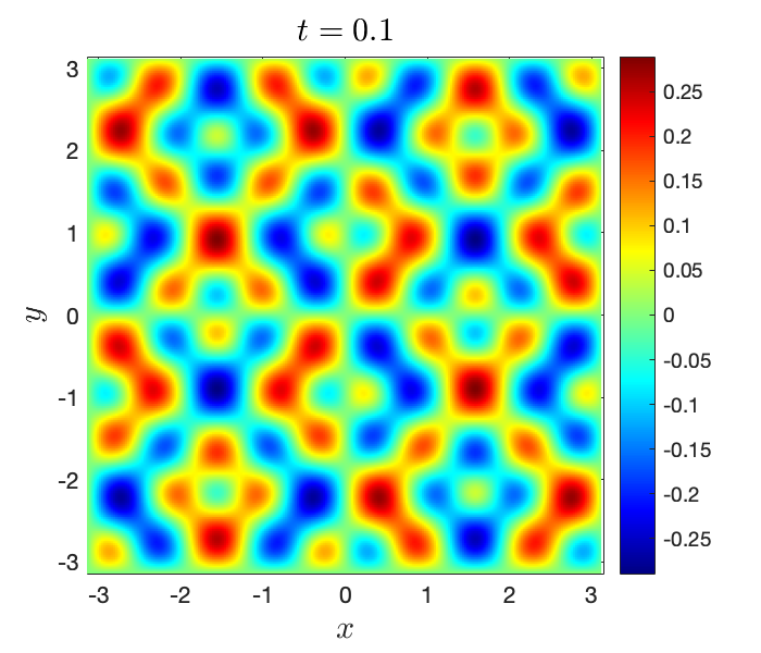
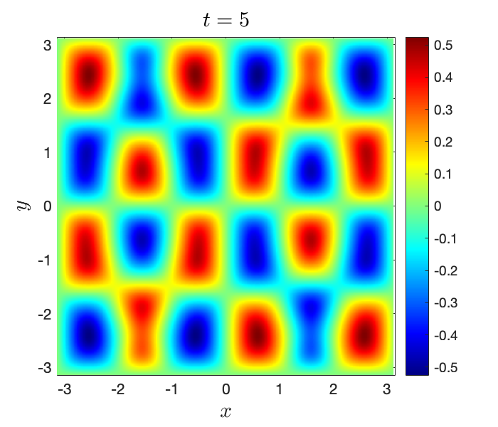
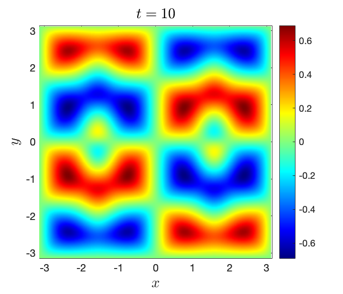
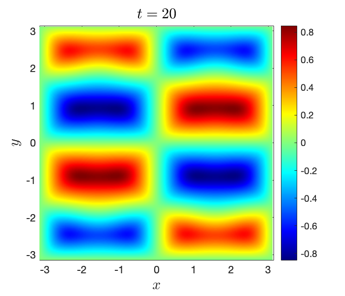
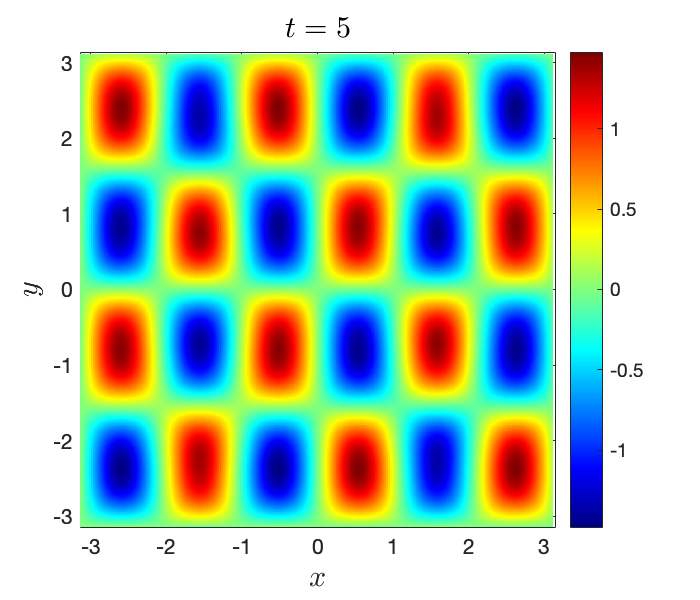
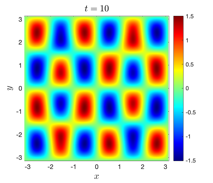
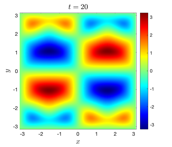
Figure 2. Example 7.1: Dynamics of 2D classical MBE equation (7.1) using the first-order IMEX scheme where $\eta=0.1,~{}\tau=0.001,~{}N_{x}=N_{y}=256$.

Figure 3. Example 7.1: Dynamics of 2D sinc-type MBE equation (7.2) using the first-order IMEX scheme where $\eta=0.1,~{}\tau=0.001,~{}N_{x}=N_{y}=256$.

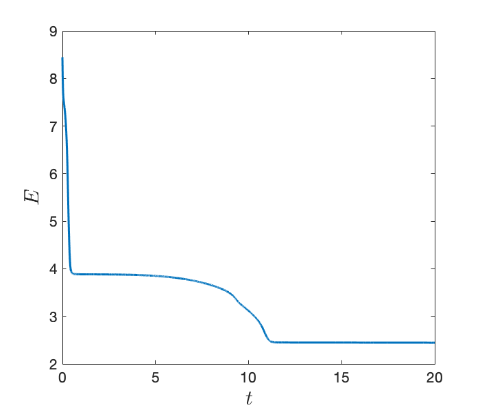
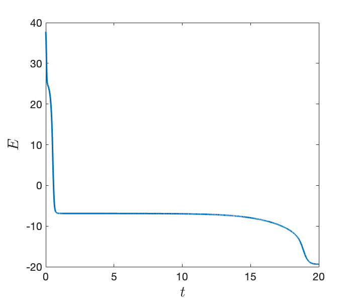
Figure 4. Example 7.1: Energy evolutions of 2D classical MBE equation (7.1) (left) and the sinc-type MBE equation (7.2) (right) computed by the first-order IMEX scheme where $\tau=0.001,~{}N_{x}=N_{y}=256$.

Secondly, we compare the energy evolutions of the classical MBE and the sinc-type MBE for different time step $\tau$ (see Figure 5). It is observed that for the classical MBE model, the energy of IMEX scheme will blow up when $\tau\geq 0.1$. However, for the sinc-type MBE model, the energy will not blow up (despite of the oscillation) even when $\tau=10$. This is consistent with our analysis on uniform boundness (cf. Theorem 4.1).

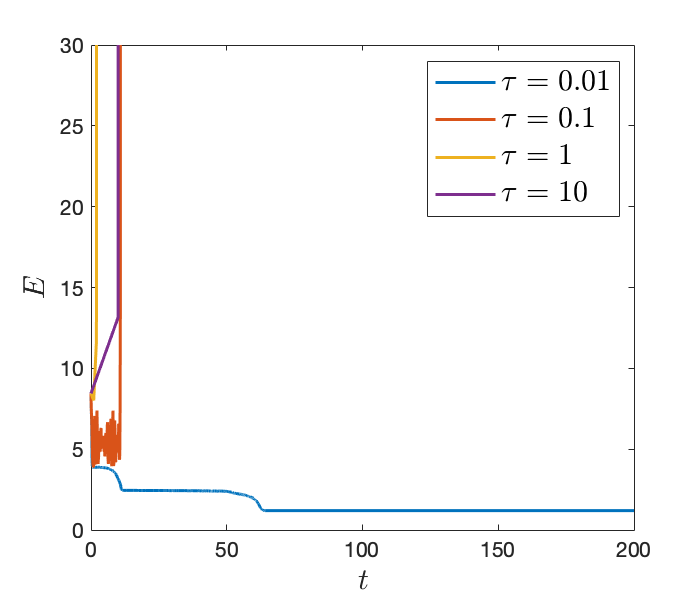
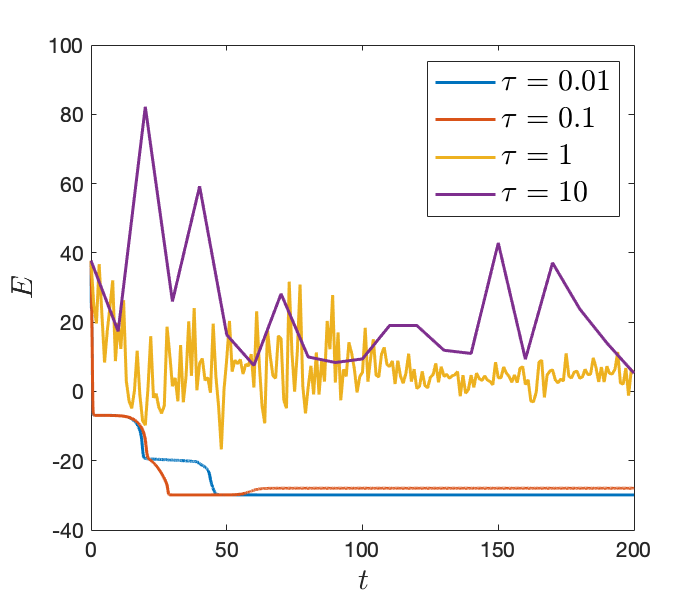
Figure 5. Example 7.1: Energy blowup phenomenon of 2D classical MBE equation (7.1) (left) and no energy blowup of the sinc-type MBE equation (7.2) (right) for different $\tau$, computed by the first-order IMEX scheme with $N_{x}=N_{y}=256$.

Thirdly, in Table 1, we compare the threshold $\tau_{\mathrm{c}}$ of time step preserving the energy dissipation, for the classical and sinc-type MBE models with different quantities of $\eta$ and different numerical schemes. To be precise, we say that the energy dissipation is not preserved if there exists $0<t_{n}\leq T$ such that

$$E^{n}-E^{n-1}\geq{\texttt{Tol}}=10^{-12},$$ (7.3)

where Tol is taken to be a mediocrely small positive number because we take account of machine error. As a consequence, $\tau_{\mathrm{c}}$ is defined by

$$\tau_{\mathrm{c}}=\sup\left\{\tau>0\mid E^{n}<E^{n-1}+{\texttt{Tol}},~{}\forall~{}0<t_{n}\leq T\right\}.$$ (7.4)

It can be observed in Table 1 that the sinc-type MBE model seems to always have larger threshold $\tau_{\mathrm{c}}$ than the classical MBE model. According to Theorem 3.1, for the IMEX scheme of sinc-type MBE model, the following inequality shall hold

$$\tau_{\mathrm{c}}\geq 8\eta^{2},$$ (7.5)

which is verified by Table 1. Similarly, according to Theorem 5.1, for the BDF2 scheme of sinc-type MBE model, the following inequality shall hold

$$\tau_{\mathrm{c}}\geq\frac{8}{9}\eta^{2},$$ (7.6)

which is also verified by Table 1.

Table 1. Threshold $\tau_{\mathrm{c}}$ of time step preserving energy dissipation, for the classical MBE and sinc-type MBE where $T=200$.

	IMEX		BDF2
$\eta^{2}$	classical	sinc-type	classical	sinc-type
$0.1$	$0.6<\tau_{\mathrm{c}}<0.7$	$1<\tau_{\mathrm{c}}<2$	$0.01<\tau_{\mathrm{c}}<0.02$	$0.06<\tau_{\mathrm{c}}<0.07$
$0.01$	$0.01<\tau_{\mathrm{c}}<0.02$	$0.09<\tau_{\mathrm{c}}<0.1$	$0.003<\tau_{\mathrm{c}}<0.004$	$0.02<\tau_{\mathrm{c}}<0.03$
$0.001$	$0.001<\tau_{\mathrm{c}}<0.002$	$0.008<\tau_{\mathrm{c}}<0.009$	$0.0003<\tau_{\mathrm{c}}<0.0004$	$0.001<\tau_{\mathrm{c}}<0.002$

Example 7.2.

Consider the following 2D sinc-type MBE equation for the growth on square symmetry surfaces

$$\partial_{t}h=-\eta^{2}\Delta^{2}h-(\sin(h_{x}))_{x}-(\sin(h_{y}))_{y},\quad\mbox{on }\mathbb{T}^{2}=[-\pi,\pi]^{2},$$ (7.7)

where $\eta=0.1$ and the initial condition is a random state by assigning a random number varying from $-0.01$ to $0.01$ to each grid point.

The model (7.7) is derived from replacing $(1-|h_{x}|^{2})h_{x}$ and $(1-|h_{y}|^{2})h_{y}$ by $\sin(h_{x})$ and $\sin(h_{y})$ respectively in the classical MBE equation for the growth on square symmetry surfaces (cf. [37]). As a consequence, the energy functional of (7.7) is defined by

$$\mathcal{E}=\int_{\Omega}\Bigl{(}\frac{1}{2}\eta^{2}|\Delta h|^{2}+\cos(h_{x})+\cos(h_{y})\Bigr{)}dx,$$ (7.8)

We solve the sinc-type MBE equation (7.7) using the following BDF2 scheme: $\forall n\geq 1$,

$$\frac{3h^{n+1}-4h^{n}+h^{n-1}}{2\tau}=-\eta^{2}\Delta^{2}h^{n+1}-2\nabla\cdot(\sin(h_{x}^{n}),\sin(h_{y}^{n}))+\nabla\cdot(\sin(h_{x}^{n-1}),\sin(h_{y}^{n-1})),$$ (7.9)

where the time step $\tau=0.01$. In Figure 6, the isolines of the free energy

$$F=\frac{1}{2}\eta^{2}|\Delta h|^{2}+\cos(h_{x})+\cos(h_{y})$$ (7.10)

are plotted at different time. The corresponding energy evolution is plotted in Figure 7. It can be observed that the energy dissipation property is preserved.

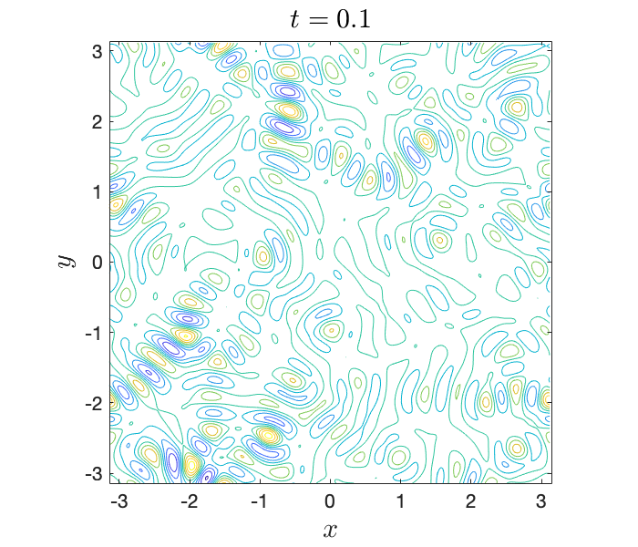
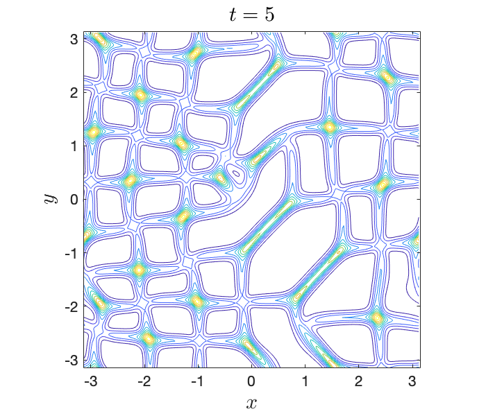
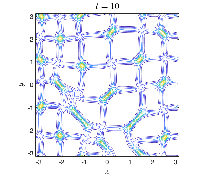
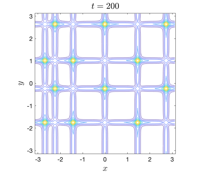
Figure 6. Example 7.2: Isolines of the free energy $F$ in (7.10) at different time for the sinc-type MBE model (7.7), computed by the BDF2 scheme (7.9) with $\tau=0.01$, $N_{x}=N_{y}=256$.

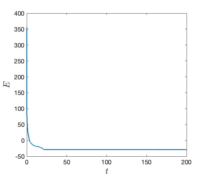
Figure 7. Example 7.2: Energy evolution of the BDF2 scheme (7.9) with $\tau=0.01$, $N_{x}=N_{y}=256$.

8. Concluding remarks

In this work we introduced a new molecular beam epitaxy model driven by a cosine-type free energy. The energy landscape of the new free energy is similar to the classical double-well potential case but has the additional advantage that all its derivatives are uniformly bounded. We analyzed two types of numerical discretization: one is the 1st order IMEX method, and the other is BDF2 in time with explicit treatment of the nonlinear term. We characterized nearly optimal time step constraints for both the first order and the second order schemes, and showed energy dissipation in both cases. We introduced two methods to show that the the energy of the numerical solutions in both schemes are unconditionally uniformly bounded, i.e. the obtained upper bound is independent of the time step. To our best knowledge, this kind of results are the first in the literature. We also carried out several numerical experiments which show that this new model is far more superior than the existing double well type MBE models. It is expected that our new theoretical framework can be generalized to many other phase-field models with good Lipschitz type nonlinearities. In addition it will be interesting to investigate the performance of other numerical schemes on the new model as well as the structural stability/instability of the metastable states and steady states.

Acknowledgement. The research of D. Li is supported in part by Hong Kong RGC grant GRF 16307317 and 16309518. The research of W. Yang is supported by NSFC Grants 11801550 and 11871470. The research of C. Quan is supported by NSFC Grant 11901281, the Guangdong Basic and Applied Basic Research Foundation (2020A1515010336), and the Stable Support Plan Program of Shenzhen Natural Science Fund (Program Contract No. 20200925160747003).

References

- [1] J.R. Arthur. Molecular beam epitaxy. Surface science. 500(1-3), (2002), 189-217.
- [2] A.L. Barabási, H.E. Stanley. Fractal Concepts in Surface Growth, Cambridge University Press, Cambridge, UK, 1995.
- [3] J. Bourgain, D. Li. Strong ill-posedness of the incompressible Euler equation in borderline Sobolev spaces, Invent. Math. 201 (2015), pp. 97-157.
- [4] S. Clarke, D.D. Vvedensky, Origin of reflection high-energy electron-diffraction intensity oscillations during molecular-beam epitaxy: A computational modeling approach. Phys. Rev. Lett. 58 (1987), pp. 2235-2238.
- [5] A.Y. Cho, J.R. Arthur. Molecular beam epitaxy. Progress in solid state chemistry. 10, (1975), 157-191.
- [6] S. Das Sarma, S.V. Ghaisas. Solid-on-solid rules and models for nonequilibrium growth in dimensions. Physical Review Letters. 69 (26), 1992, 2651-2654.
- [7] S. Das Sarma, C.J. Lanczycki, R. Kotlyar, S.V. Ghaisas. Scale invariance and dynamical correlations in growth models of molecular beam epitaxy. Physical Review E, 53(1), (1996), 359-388.
- [8] G. Ehrlich, F.G. Hudda, Atomic view of surface diffusion: Tungsten on tungsten. J. Chem. Phys. 44 (1966), pp. 1039-1049.
- [9] L. Golubović. Interfacial coarsening in epitaxial growth models without slope selection. Phys. Rev. Lett. 78 (1), (1997), 90-93.
- [10] C. Herring. Surface tension as a motivation for sintering In: Kingston, W.E. (Ed.) The Physics of powder Metallurgy, McGraw-Hill, New York.
- [11] M.D. Johnson, C. Orme, A.W. Hunt, D. Graff, J. Sudijono, L.M. Sander, B.G. Orr. Stable and unstable growth in molecular beam epitaxy. Physical review letters. 72(1), (1994), 116-119.
- [12] J.M. Kim, S. Das Sarma. Discrete models for conserved growth equations. Physical review letters. 72(18), (1994), 2903-2906.
- [13] R. Kohn, S. Müller. Surface energy and microstructure in coherent phase transitions. Comm. Pure Appl. Math. 47, (1994), 405-435.
- [14] R. Kohn, X. Yan. Upper bounds on the coarsening rate for an epitaxial growth model. Comm. Pure Appl. Math. 56(11), (2003), 1549-1564.
- [15] J. Krug, Origins of scale invariance in growth processes. Adv. in Phys. 46 (1997), pp. 139-282.
- [16] B. Li, J.G. Liu. Thin film epitaxy with or without slope selection. European Journal of Applied Mathematics, 14(6) (2003), 713-743.
- [17] Z.W. Lai, S. Das Sarma. Kinetic growth with surface relaxation: Continuum versus atomistic models. Physical review letters, 66(18), (1991), 2348-2351.
- [18] D. Li. On a frequency localized Bernstein inequality and some generalized Poincaré-type inequalities. Mathematical Research Letters. 20.5 (2013): 933-945.
- [19] D. Li, Z.H. Qiao, T. Tang. Characterizing the stabilization size for semi-implicit Fourier-spectral method to phase field equations. SIAM J. Numer. Anal. 54 (2016), no. 3, 1653-1681.
- [20] D. Li, Z.H. Qiao, T. Tang. Gradient bounds for a thin film epitaxy equation. Journal of Differential Equations, 262 (2017), no. 3, 1720-1746.
- [21] D. Li, F. Wang, K. Yang. An improved gradient bound for 2D MBE. Journal of Differential Equations, 269.12 (2020): 11165-11171.
- [22] D. Li, T. Tang. Stability of the Semi-Implicit Method for the Cahn-Hilliard Equation with Logarithmic Potentials. Ann. Appl. Math., 37 (2021), 31-60.
- [23] D. Li, T. Tang. Stability analysis for the Implicit-Explicit discretization of the Cahn-Hilliard equation. arXiv:2008.03701.
- [24] W.W. Mullins. Theory of thermal grooving. Journal of Applied Physics. 28(3), (1957), 333-339.
- [25] L. Onsager. Reciprocal relations in irreversible processes. I. Physical review. 37(4), (1931), 405-426.
- [26] L. Onsager. Reciprocal relations in irreversible processes. II. Physical review. 38(12), (1931), 2265-2279.
- [27] M. Ortiz, E. Repetto, H. Si. A continuum model of kinetic roughening and coarsening in thin films. J. Mech. Phys. Solids. 47, (1999), 697-730.
- [28] R.K. Pathria, P.D. Beale. Statistical mechanics, 1996. Butter worth, 32.
- [29] P. Politi, G. Grenet, A. Marty, A. Ponchet, J. Villain. Instabilities in crystal growth by atomic or molecular beams. Phys. Reports, 324, (2000), 271-404.
- [30] P. Politi, J. Villain. Ehrlich-Schwoebel instability in molecular-beam epitaxy: A minimal model. Phys. Rev. B, 54(7), (1996), 5114-5129.
- [31] M. Schneider, I.K. Schuller, A. Rahman, Epitaxial growth of silicon: A moleculardynamics simulation. Phys. Rev. B, 36 (1987), pp. 1340-1343.
- [32] J. Shen and X. Yang. Numerical approximations of Allen-Cahn and Cahn-Hilliard equations. Discrete Contin. Dyn. Syst. A, 28 (2010), 1669–1691.
- [33] J. Shen, C. Wang, X. Wang, S.M. Wise. Second-order convex splitting schemes for gradient flows with Ehrlich-Schwoebel type energy: Application to thin film epitaxy. SIAM J. Numer. Anal., 50 (2012), pp. 105-125.
- [34] M. Siegert, M. Plischke. Slope selection and coarsening in molecular beam epitaxy. Phys. Rev. Lett. 73(11), (1994), 1517-1520.
- [35] H. Song and C.W Shu. Unconditional Energy Stability Analysis of a Second Order Implicit-Explicit Local Discontinuous Galerkin Method for the Cahn-Hilliard Equation. Journal of Scientific Computing. volume 73 (2017), pages 1178–1203.
- [36] J. Villain, Continuum models of critical growth from atomic beams with and without desorption, J. Phys. I., 1 (1991), pp. 19-42.
- [37] C.J. Xu, T. Tang. Stability analysis of large time-stepping methods for epitaxial growth models. SIAM J. Numer. Anal. 44 (2006), no. 4, 1759-1779.
- [38] A. Zangwill. Theory of growth-induced surface roughness. In: Hatwater, H.A., Thompson, C. (Eds.), Microstructural Evolution of Thin Films. Academic Press, New York.
- [39] A. Zangwill. Some causes and a consequence of epitaxial roughening. Journal of Crystal Growth. 163, (1996), 8-21.