Statistics of drops generated from ensembles of randomly corrugated ligaments

Abstract

The size of drops generated by the capillary-driven disintegration of liquid ligaments plays a fundamental role in several important natural phenomena, ranging from heat and mass transfer at the ocean-atmosphere interface to pathogen transmission. The inherent non-linearity of the equations governing the ligament destabilization lead to significant differences in the resulting drop sizes, owing to small fluctuations in the myriad initial conditions. Previous experiments and simulations reveal a variety of drop size distributions, corresponding to competing underlying physical interpretations. Here, we perform numerical simulations of individual ligaments, the deterministic breakup of which is triggered by random initial surface corrugations. Stochasticity is incorporated by simulating a large ensemble of such ligaments, each realization corresponding to a random but unique initial configuration. The resulting probability distributions reveal three stable drop sizes, generated via a sequence of two distinct stages of breakup. The probability of the large sizes is described by volume-weighted Poisson and Log-Normal distributions for the first and second breakup stages, respectively. The study demonstrates a precisely controllable and reproducible framework, which can be employed to investigate the mechanisms responsible for the polydispersity of drop sizes found in complex fluid fragmentation scenarios.

I Introduction

Liquid fragmentation is the transformation of a compact volume into drops. The simplest example is the capillary-driven breakup of a slender cylindrical structure [1] at approximately regular intervals driven via the growth of long wavelength perturbations [2, 3, 4]. A slightly complicated transition involves expanding liquid sheets [5, 6], where the inertial expansion opposed by the capillary deceleration of the edges results in the formation of liquid rims, the subsequent destabilization of which leads to drops. Alternatively in perforated liquid sheets, the rapid capillary-driven expansion of the perforations [7, 8] form an interconnected set of filaments, which eventually break into drops. Arguably, the most convoluted topological changes are encountered when macroscopic liquid structures (e.g. jets, mixing layers) are subjected to high shear rates [9, 10], where Kelvin-Helmholtz [11] type instabilities generate many of the aforementioned structures like filaments, expanding sheets with rims, thin sheets with expanding holes etc. The only common feature that unites these seemingly disparate fragmentation processes is that the penultimate topological stage of drop formation is constituted by cylindrical thread-like structures called ligaments.

The size of drops resulting from the breakup of ligaments governs physical mechanisms underlying a broad range of natural processes and industrial applications. These processes include (but not limited to) the exchange of heat and mass transfer at the ocean-atmosphere interface [12, 13], mixing/separation in metallurgical applications [14, 15], pesticide dispersal and irrigation in industrial agriculture [16, 17, 18], and ever so important, pathogen transmission driven by violent respiratory events [19, 20]. Therefore, the development of quantitative models geared towards statistical predictions of the size and velocity of drops has drawn considerable scientific interest [21] over the recent decades.

Several experimental and numerical investigations of drop size statistics have led to the popularization of three distinct classes of probability density functions, namely the Log-normal, Gamma and Poisson distributions, as outlined in the review by Villermaux [22]. In addition, distributions such as the Gaussian [6], Weibull [23], Exponential [24] and Beta [25] have also received significant attention. Regarding the interpretation of the underlying physical mechanisms, the Log-normal model [26] implies a sequential cascade of breakups (analogous to the Kolmogorov [27] energy cascade in fluid turbulence), the Gamma family [28] considers the competing effects of fragmentation and cohesion, and the Poisson model [29] entails instantaneous and random splitting of a volume into smaller fragments. These models have been used in a diverse range of fragmentation scenarios to varying degrees of predictive success, however, there is a general lack of consensus regarding their generalization. This is primarily due to the fact that the initial liquid structures follow markedly different dynamical trajectories towards drop formation, rendering certain models incompatible with the actual physical mechanism at play (refer to [6] for a discussion).

I.1 Modes of ligament breakup

The topological change from the threadlike ligaments to the (approximately) spherical geometry of drops can proceed along different paths, depending on the relative importance of viscosity and surface tension, the aspect-ratio, and the strength of the initial perturbation [30, 31, 32, 33]. Extremely viscous ligaments are stable against capillary-driven disintegration [34]. For intermediate viscosities, the ligament ruptures at several locations along its length primarily due to the Rayleigh-Plateau instability [32]. In low-viscosity regimes, the ligament might also fragment from one of its free ends, referred to as the end-pinching mode [35, 36]. Additionally, if the ligament is free at both ends and not slender enough (small aspect-ratios), the capillary retraction might dominate and contract the entire volume into a single drop [37]. Thus, despite the richness of end-pinching dynamics and complete contraction, the resulting drop sizes are extensively documented and well described by robust scaling laws [35, 30, 38]. This turns our attention solely towards the drops formed due to breakups along the ligament length.

The mechanism of the liquid-thread rupture leading to drop formation is essentially self-similar [39, 40], corresponding to finite-time singularities of the Navier-Stokes equations. Although this universality renders the pinching process insensitive to the initial conditions of the ligament, the liquid rearrangements within the ligament bulk are sensitive to the initial conditions, owing to the inherent non-linearities in the governing equations. The final arrangement of liquid volumes just prior to the rupture of the liquid-thread directly correlates to the volume contained in the drops formed. Therefore, having precise quantitative control over the ligament initial conditions is of paramount importance in order to understand the polydispersity in the resulting drop sizes.

I.2 Our computational framework

Towards this objective, the central theme of this study is the design and conception of “numerical” experiments, that lend themselves to accurate and repeatable specifications of the initial conditions of the ligaments in question. Generally in physical experiments, obtaining ligaments conforming exactly to a specified geometrical shape and velocity field is extremely challenging. Thus, one often has to employ a posteriori correlations between the observed dispersion in the final drop sizes and the “qualitative” descriptions of initial conditions. In contrast, our present numerical framework allows us to obtain reproducible drop size distributions, which are purely outcomes of the mathematical model (Navier Stokes with surface tension), subject to a chosen set of parameters, initial and boundary conditions. Furthermore, most of the reported drop size distributions in experiments incorporate significant uncertainties, owing to small sample sizes. In our case, we are able to precisely control the degree of uncertainty in our eventual distributions, as the rapid calculation times enables us to generate large statistical samples.

II Methodology

II.1 Mathematical Model

We use the one-fluid formulation for our system of governing equations, thus solving the incompressible Navier-Stokes equations throughout the whole domain, including regions of variable density and viscosity which itself depend on the explicit location of the interface separating the two fluids [41]. The interface is modeled as having an infinitesimal thickness at the macroscopic scales under consideration. The temporal evolution of the interface is tracked by using an advection equation for the phase-characteristic function, which is essentially a Heaviside function that distinguishes the individual phases. The density and viscosity at each spatial location are expressed as linear functions of the phase-characteristic function.

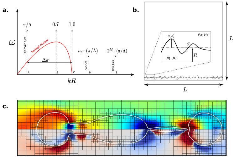
Figure 1: a. Variation of the linearized growth rate ($\omega$) corresponding to the viscous Rayleigh-Plateau instability obtained by Weber [42], as a function of nondimensional wavenumber $kR$. In our setup, $n_{c}$ discrete wavelengths are excited as part of the initial condition, which fall within the vertical lines $A$ and $D$. Only a certain number of these $n_{c}$ discrete modes are unstable ($\omega>0$) with respect to the Rayleigh-Plateau instability (red curve, between vertical lines $A$ and $C$). The number of such unstable modes ($\Delta k$) scales linearly with the size of the ligament ($\Delta k\sim\Lambda/\pi$). The vertical line $B$ represents the approximate value of $kR$ for which we get the optimal growth rate. b. Schematic of the computational setup. An infinitely long and axisymmetric corrugated ligament of mean radius $R$ is placed along a side of a square domain of size $L$. The bottom side of the box acts as the axis of symmetry, while spatial periodicity is imposed along the horizontal direction. Inset : A close up view of the corrugated profile of the ligament, where the local radius is defined as the sum of the unperturbed (mean) radius $R$ and the local perturbation $\epsilon(x)$. The material properties of the liquid and gas phases are denoted with the subscripts $l$ and $g$ respectively, which in our case corresponds to an air-water system with the surface tension coefficient $\sigma$. c. Dynamically adapted octree meshes in the periphery of the interface location, with the refinement criteria based on limiting second gradients (curvatures) of the volume fraction and velocity fields. The interface is represented by the white contours, the colormap on the left half is based on the axial velocity component, whereas the one on the right corresponds to that of vorticity. The colors red and blue correspond to the higher and lower end values respectively, in case of both colormaps.

II.2 Numerical Methods

We use the free software (scientific computing toolbox) Basilisk [43, 44, 45], which couples finite-volume discretization with adaptive octree meshes (see fig. 1c) in order to solve our governing partial differential equations. The interface evolution is tracked using a Volume-of-Fluid (VOF) method [46, 47], coupled with a robust and accurate implementation of height-function based interface curvature computation [48]. The capillary forces are modeled as source terms in the Navier-Stokes equations using the continuum surface-force [49] (CSF) method.

In our present context of ligament destabilization, the trajectory of the system towards drop formation is governed by non-linear interactions between capillary waves, remnants of the internal flow, acceleration of the liquid into the surrounding medium, localized vorticity production at the interface, as well as viscous dissipation in the bulk. In order to accurately reproduce the aforementioned multiscale phenomena and ensure sufficient spatio-temporal resolution in the vicinity of breakups and coalescence, the dynamically adaptive octree meshes (Fig. 1c.) are absolutely essential in order to carry out computationally efficient simulations. The accuracy and performance of Basilisk has been well documented and extensively validated for a variety of complex interfacial flows such as breaking waves [50, 51, 52], bursting bubbles [53, 54], drop splashes [55], amongst many others.

II.3 Computational Setup

We conduct direct numerical simulations of air-water systems consisting of slender ligaments with spatial periodicity along the axis ligament axis. The absence of free ends (periodically infinite ligaments) in the initial condition ensures that the end-pinching mode is suppressed during the initial dynamics of the system, although this mode may come into play once the ligament breaks up into smaller fragments having free ends.

As a simplification, we use an axisymmetric framework (3D) that excludes all azimuthal variations in the shape of the ligament and subsequently formed drops. Fig. 1b illustrates the schematic of the computational setup, where the domain is a square of side $L$. The bottom side of the box acts as the axis of symmetry for the corrugated ligament (detailed view in the inset of Fig. 1b), which has an unperturbed (mean) radius $R$. The radial profile $R(x)$ along the ligament axis can be written as $R(x)=R+\epsilon(x)$, where $\epsilon(x)\sim\mathcal{N}\left(0,\varepsilon^{2}_{0}\right)$. Periodic boundary conditions are imposed for the primary variables on the left and right faces of the domain. Symmetry boundary conditions are imposed on the bottom side, with the impenetrable free-slip condition applied to the top side.

II.3.1 Random Surface Generation

The random surfaces of our spatially periodic ligaments are constructed by taking a white noise signal, (using a robust random number generator [56]) which is subsequently filtered (keeping only longest $n_{c}=25$ wavelengths) in order to generate the final radial profile of the ligament with variance $\varepsilon_{0}^{2}$. The exact surface profile of an individual ligament in the ensemble is precisely and uniquely determined by the “seed” (state) of the random number generator [56], thus allowing us to create an ensemble of such random but unique surface profiles by mapping each profile to unique values of the seed. In the case of infinitely long ligaments, only perturbations with wavelengths larger than the ligament circumference are unstable to the Rayleigh-Plateau [2, 3] type capillary instability. Owing to the discrete nature of numerical simulations, we are only able to initially excite a finite and small number of discrete modes that fall within the unstable part of the spectrum (see fig. 1a). The number of such unstable discrete modes varies linearly with the aspect-ratio ($\Delta k\sim\Lambda/\pi$), therefore, in our case we have $15$ discrete unstable modes, including a few close to the optimally perturbed Rayleigh-Plateau wavelength.

II.3.2 Regime of Interest

In order to isolate the influence of initial geometrical shape on the subsequent dynamics and drops formed, we exclude inertial forces (axial stretching rate) in our initial conditions. The mean radius $R$ of the ligament is the characteristic length scale of the problem. As we are dealing with air-water systems (20 degrees Celsius), the density and viscosity ratios are given as $\rho_{l}/\rho_{g}\simeq 830$ and $\mu_{l}/\mu_{g}\simeq 45$ respectively. Thus, our system is characterized by the Ohnesorge number which is defined as

$$\textrm{Oh}=\mu/\sqrt{\rho\sigma R}\,.$$ (1)

The Ohnesorge number is simply the square-root of the ratio of the viscous length scale ($l_{\mu}=\mu^{2}/\rho\sigma$) with the characteristic length scale of the problem ($R$). Although the configuration initially has no kinetic energy, a part of the surface potential is immediately converted into liquid inertia as soon as the system is released from its static initial conditions. Hence, we can interpret this balance as $\textrm{We}\to 1$, where We is the Weber number, defined as the ratio of inertial and capillary forces. The geometrical shape of any individual ligament in our ensemble is characterized by a mean corrugation amplitude $\eta=\varepsilon_{0}/R$, and aspect-ratio $\Lambda=L/W$, where $W=2R$ denotes the mean width of the ligament. The volume of the corrugated ligament per unit spatial period ($L$) is controlled by $\Lambda$, which also acts as the theoretical upper bound to the drop size. Additionally, we rescale physical time with the capillary time scale such that $T=t/t_{\sigma}$, where $t_{\sigma}=\left(\rho R^{3}/\sigma\right)^{-1/2}$. The material properties used in our adimensional parameters ($\rho$, $\mu$) correspond to the liquid phase i.e. water. In the present study, we focus our attention on weakly perturbed ($\eta\simeq 0.08$) and sufficiently slender ligaments ($\Lambda\simeq 50$) at the characteristic length scale of $100$ microns ($\textrm{Oh}\simeq 10^{-2}$).

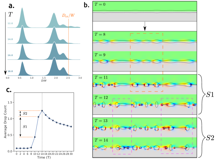
Figure 2: a. Temporal evolution of the probability density functions of drop size, where drop size is expressed as diameter rescaled by the initial ligament width $W$. Across time, the distribution peaks reveal 3 stable drop sizes, namely the satellite drops ($D/W\simeq 0.6$), primary drops ($D/W\simeq 1.9$) and secondary drops ($D/W\simeq 2.3$). The number of satellite drops decreases with time due to coalescence with adjacent larger drops. On the other hand, the secondary drops grow in number as time progresses, due to the continuous breakup of the elongated drop-like structures having aspect-ratios above the critical threshold ($\Lambda_{\textrm{cr}}/W\sim(D_{\textrm{cr}}/W)^{3}$) . These elongated structures generally break up into primary or secondary drops. b. Destabilization of a ligament (closeup view showing 3/4 of the ligament length) randomly selected from our ensemble, demonstrating the different breakup stages. The interface shape is represented by the black contours. The colormaps of the top and bottom halves in each plot (snapshot in time) represent the axial velocity component and the magnitude of vorticity, respectively. In both colormaps, red and blue correspond to the higher and lower end values respectively. Both colormaps have an identical range ($-1$ to $1$) across all temporal snapshots, where the original range of each individual plot (e.g $T=12$) is normalized by the minimum and maximum values of the respective fields across all temporal snapshots shown. In snapshots $T=8,9$, we observe the formation of drops (within the orange dashed box) corresponding to the optimally perturbed wavelength of the Rayleigh-Plateau instability. This leads to the first stage of breakups (S1), where the ligament disintegrates into primary, satellite and secondary drops, along with some elongated structures larger than the secondary drops. Subsequently, we enter the second stage of breakups (S2), where the elongated structures themselves disintegrate into smaller sizes (within purple dashed boxes), typically into primary and secondary drops. c. The average number of drops generated through the disintegration of the ligaments in our ensemble, mapped as a function of time. The slope of the curve is governed by the difference between the number of ”breakup” and ”coalescence” events at any instant of time. A limited number of breakups occur before $T=6$. Starting from $T=8$, breakup events occurring on much faster timescales dominate coalescence, thus rapidly leading to a peak in number of drops generated at $T=14$. Between $T=8$ and $T=14$, there are two distinct stages of breakup represented by S1 and S2. Beyond $T=14$, the number of breakup events is significantly less than coalescence, thus leading to the average drop count decreasing over a slower timescale.

III Results

The process of drop formation via ligament breakup is deterministic, therefore it is completely characterized by the initial (exact) geometrical shape of the ligament. Stochasticity is introduced to the mix by creating an ensemble of such corrugated ligaments, where each individual ligament has a random but unique surface, while ensuring that the statistical properties ($\eta$) of the corrugated shape are identical across all ligaments in the ensemble. This key step allows us to incorporate the effects of the myriad underlying processes that determine the exact ligament shape in realistic fragmentation scenarios, that too in a quantitatively precise and reproducible manner.

III.1 Statistics of Drop Formation

In Fig. 2b, we illustrate the different stages involved in the breakup of an individual ligament into drops, where the ligament is randomly selected from our ensemble of size $10000$. Linear theory based on the Rayleigh breakup [2, 3] of infinitely long liquid cylinders in a quiescent medium predict the initial destabilization phase (panels $T=8$, $T=9$ of fig. 2b) proceeding via exponential growth of the different (unstable) discrete frequencies that constitute the initial surface perturbation. Beyond this linear growth phase, non-linearities rapidly kick in near the breakup zones [57, 58, 1], eventually resulting in the formation of “main” and significantly smaller “satellite” droplets , as observed in panels $T=11$, $T=12$ of fig. 2b. In our study, we refer to this as the first stage of breakups (S1), where we find a set of “primary” and “satellite” drops (orange dashed box in fig. 2b), along with a collection of strongly deformed elongated structures (purple dashed box in fig. 2b) which themselves resemble small aspect-ratio ligaments. This stage is immediately followed by the second stage of breakups (S2), in which the elongated structures break down into smaller fragments, while the previously formed primary and satellite drops remain stable.

The number of drops in our ensemble is measured using average drop count, which is defined as the ratio of the total number of drops in the ensemble and the total units of a characteristic length, across the entire ligament ensemble. The characteristic length is chosen as the wavelength ($\lambda_{\text{RP}}=2\pi/k_{\text{RP}}\simeq 9R$) corresponding to the optimal growth rate of the viscous Rayleigh-Plateau instability [42, 2, 3]. In Fig. 2a, we plot the temporal variation of average drop count. The slope of the graph is determined by the competition between breakup and coalescence events, thus delineating the 2 distinct stages of breakup (S1 and S2), as well as the dominance of coalescence events beyond $T=14$, leading to a slow decrease in the number of drops.

Coming to the statistics of drop sizes , in fig. 2a, we show the probability density functions (PDF) corresponding to drop size distributions as a function of time. The drop diameters are rescaled by the initial width ($W$) of the ligaments. One can clearly observe the presence and persistence of three distinct peaks in the size distribution for all instants of time shown. These stable peaks correspond to drop sizes given by $D/W\simeq 0.6$ for the satellite drops, $D/W\simeq 1.9$ for the primary drops, and $D/W\simeq 2.3$ for what we refer to as “secondary” drops.

Assuming that drops are formed by encapsulating the volume of liquid contained within one optimally perturbed wavelength ($2\pi/k_{\text{RP}}$), we can compute the diameter $D_{\text{RP}}$ as

$$\frac{\pi}{6}D_{\text{RP}}^{3} =\frac{\pi}{4}W^{2}\left(2\pi/k_{\text{RP}}\right)$$

$$\implies D_{\text{RP}}/W \simeq 1.89\,.$$ (2)

As we can observe in fig. 2a, the statistical estimate of our primary drop size (values distributed around $D/W\simeq 1.9$) across time is in excellent agreement with the predictions (2) of linearized stability theory.

The typical size of satellite drops has a strong dependence on the initial conditions, as meticulously documented in the seminal work of Ashgriz & Mashayek [59] concerning the capillary breakup of jets. In that study, the authors report a monotonic decrease in the satellite drop size as one increases the initial perturbation strength (fig. 12 in [59]). At the limit of vanishing perturbation strength (matching our initial conditions), Ashgriz & Mashayek obtain a satellite drop size of $D/W\simeq 0.6$, which matches quite well with the statistical observations of our satellite drop size (fig. 2a).

Immediately after the first set of breakups (S1), there are plenty of elongated structures with free ends (including our “secondary” drops), which might be subject to the end-pinching mechanism. Several numerical, experimental and scaling analyses in existing literature (Shulkes [30], Gordillo & Gekle [38] ,Wang & Bourouiba [6]) have established that the size of drops generated via the end-pinching mechanism are deterministically characterised by the width of the ligament of origin, given by a near constant value of $D/W\simeq 1.5$ (although with an extremely weak dependence on inertial stretching rate). Therefore, the absence of any peak in our drop size statistics (fig. 2a) after $T=12$ (beyond S1) around the value $D/W\simeq 1.5$ is a striking observation, asserting that negligible breakups occur via the end-pinching mode. Further investigations must be conducted in order to establish the exact cause of this absence.

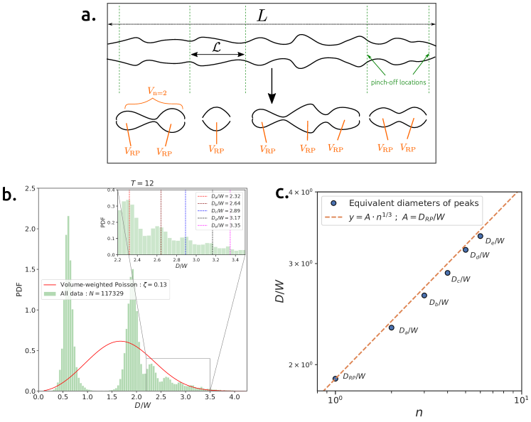
Figure 3: a. A toy model representation of the dynamics during the first stage of breakups (S1). The green vertical lines on the intact ligament (top figure) denote the possible pinch-off locations along the length $L$ of the ligament, and $\mathcal{L}$ is the random variable describing the exponential spacing (Poisson model) between successive pinch-off events. Once the pinch-offs occur, the (random) volume $V_{n}$ of the “elongated drops” can be modeled as a linear combination of smaller characteristic volumes, where $V_{\rm RP}$ belongs to normal distributions centered around the expected value of volume contained under one unit of the optimally perturbed viscous Rayleigh-Plateau instability. b. Probability density function of the drop size at $T=12$, displaying the peaks corresponding to the satellite and primary drops, as well as the typical sizes of the elongated drop-like structures in the distribution tail. The volume-weighted Poisson (exponential) distribution (4) is plotted using a pinch-off rate ($\zeta=0.13$) determined by the average number of drops formed per ligament. Inset: Zoom-up on the peaks representing the typical sizes of the elongated structures. c. The predictions of our simplified model (orange dashed line) for the typical sizes of the elongated structures, plotted alongside the statistical observations of the drop sizes (blue circles) that constitute the peaks within the tail of our distribution at $T=12$. Assuming that the elongated structures are generated by encapsulating integer multiples of the characteristic volume $V_{\rm RP}$, the equivalent diameters should scale according to $D_{n}/W\sim n^{1/3}$, where $n$ is the number of characteristic units of $V_{\rm RP}$.

III.2 First Stage of Breakups (S1)

We take a closer look at the probability of the large drop sizes immediately after the first set of breakups. We start with a simple model for the ligament pinching-off at several locations, with the assumptions (i) only 1 pinch-off occurs in an infinitesimally small interval $dl$.(ii) a small, uniform and independent probability of the ligament pinching-off in each $dl$. Therefore, the total number of pinch-offs over the entire length $L$ follows a Poisson distribution, implying that the spacing $\mathcal{L}$ between any two pinch-off locations (see fig. 3b) follows an exponential distribution, with the probability density function given by

$$f_{\mathcal{L}}(x)=\zeta\cdot\textrm{exp}(-\zeta x)\,,$$ (3)

where $\mathcal{L}$ is the random variable for the exponential spacing, and $\zeta$ being the expected value of the number of pinch-offs occurring over length $L$. We set $\mathcal{D}\equiv D/W$ as the random variable representing the size of the drop formed by encapsulating the volume between two successive pinch-off locations. Using the relation $\mathcal{D}=c\mathcal{L}^{1/3}$ ($c$ is a constant), we obtain the expression for the PDF of random variable $\mathcal{D}$ as

$$f_{\mathcal{D}}(x)=\frac{3\zeta x^{2}}{c}\textrm{exp}(-\zeta x^{3}/c)\,,$$ (4)

which we refer to as the “volume-weighted” exponential (or Poisson) distribution. The pinch-off rate is determined by first calculating the rate of drops formed : $117,329\,\text{drops}/10,000\,\text{ligaments}\approx 12$ drops per ligament. Since the average number of pinch-offs is equal to one more than the average number of drops, we obtain $\zeta\simeq 0.13$ as there are 100 units of length per ligament. In fig. 3b, we plot the PDF of the drop size distribution at $T=12$, as well the volume-weighted exponential PDF using $\zeta=0.13$ (no free parameters). We observe that the tail of the distribution matches the predictions of the volume-weighted exponential model (4) quite satisfactorily, even though it cannot capture the probabilities of the primary and satellite drops.

We observe that the tail of the distribution at $T=12$ contains small peaks (see fig. 2a at $T=12$ , fig. 3b), which corresponds to some typical sizes of the elongated structures, and we seek a simplified model to to predict the size of such drops. As demonstrated in fig. 3a, each “elongated drop” (formed after the Poisson-like pinch-off events) is assumed to be a connected set of smaller characteristic volumes. The characteristic volumes are assumed to be normally distributed random variables i.e. $V_{p}\sim\mathcal{N}(\pi W^{2}L/4p,\gamma_{p})$, where $p$ represents the (Rayleigh-Plateau unstable) discrete wavelengths ($L/p$) which are excited as part of the initial condition. Opting for a further simplification, we only consider one characteristic volume $V_{\rm RP}$ with expected value $\frac{\pi}{4}W^{2}\left(2\pi/k_{\text{RP}}\right)$, thus modeling any given elongated structure to be composed of integer multiples of the volume encapsulated under optimally perturbed viscous Rayleigh-Plateau wavelength.

Thus, given that $V_{n}=n\cdot V_{\rm RP}$, the diameters corresponding to the peaks in the inset of fig. 3b should simply vary as $D_{n}/W=A\cdot n^{1/3}$, where $A=D_{\rm RP}/W$ is the Rayleigh-Plateau optimal drop size. In fig. 3c, we plot the predictions of this simple model against the statistically observed values of the peaks present in the distribution tail at $T=12$ (inset fig. 3b)) . The close agreement of our model with the statistical observations strongly suggests that the elongated structures (sizes larger than the primary drops) are simply integer multiples of the primary drops, where the number of primary drop units within one elongated structure is determined by random pinch-offs along the heavily perturbed ligament.

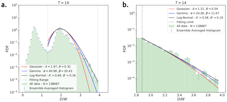
Figure 4: Drop size distributions at $T=14$, representing the drop ensemble immediately after the two stages (S1 and S2) of breakup. Averaged distributions (blue points with error bars) with $95\%$ confidence intervals are plotted on top of the distribution corresponding to the entire ensemble of size $N=138,693$ (green histogram). a. The best fits corresponding to the Gaussian, Log-Normal and Gamma distribution functions are plotted within a range (dashed vertical lines) that includes the peak representing the primary drops. We observe that the Log-Normal fit best describes the distribution over the selected range, and differences comparing the Gamma fit appear only near the tail end of the distribution. b. The best fit corresponding to the Gaussian, Log-Normal and Gamma distribution are plotted while excluding the peak representing the primary drop size. In this case, the Gamma fit appears to best describe the probabilities of the large drop sizes, but it is difficult to distinguish between each of the three candidate functions.

III.3 Second Stage of Breakups (S2)

We now turn our attention towards the fate of the large ($D/W>1.9$) “elongated” drops during the second stage of breakups. Considering these structures as small aspect-ratio ligaments, they can collapse into a single (or two) drop(s) via the capillary-driven retraction of both the ends, or break up into multiple drops along its length through a Rayleigh-Plateau type instability mechanism [32]. Driessen et al. [32] demonstrate using a combination of analytical arguments and numerical simulations, the existence of a critical aspect-ratio $\Lambda_{\text{cr}}$, below which, the structure is entirely stable against the Rayleigh-Plateau instability. This critical $\Lambda_{\text{cr}}$ is determined by equating the time taken by the optimal Rayleigh-Plateau perturbation to grow to the ligament radius, with the time taken by the two ends to retract to half the ligament length. The expression for $\Lambda_{\text{cr}}$ provided by Driessen et al. [32], but adapted to our problem setup is given as

$$\frac{|\textrm{log}(\eta^{\prime})|}{t_{\sigma}\cdot\omega_{\textrm{max}}}+\left(6\Lambda_{\text{cr}}\right)^{1/3}-\Lambda_{\text{cr}}=0\,,$$ (5)

where, $\eta^{\prime}$ indicates the degree to which the surface of the ligament (elongated drop) is perturbed. The perturbation strength corresponding to our initial condition $\eta$ acts as the lower bound to $\eta^{\prime}$ simply due to the fact that the perturbations grow as a function of time. The optimal growth rate $\omega_{\textrm{max}}$ is a function of the Ohnesorge number, and is calculated from the dispersion relation obtained by Weber [42] (fig. 1a) for the capillary instability at the low Reynolds limit of the Navier-Stokes equations (long wave approximation). Using a simple root-finding algorithm for the non-linear equation (5), with $\eta^{{}^{\prime}}=\eta$ , we obtain the critical aspect-ratio value for our setup as $\Lambda_{\text{cr}}\simeq 11.5$, which is a slight overestimation due to the fact the our elongated structures are significantly more perturbed than $\eta$. Computing the equivalent diameter for the volume contained in a ligament of mean width $W$ and aspect-ratio $\Lambda_{\text{cr}}$, we get $D_{\text{cr}}/W\simeq 2.5$.

Revisiting fig. 2a, we observe that the number (or probability) of drops lying to the right of the $D_{\text{cr}}/W$ mark (orange dashed line) decreases with time starting from $T=12$ to $T=16$. In addition, the “secondary” peak is the only one whose height does not decrease with time, rather, increases steadily with time. This observation can be explained by the continuous breakup of the elongated drops into smaller fragments, till they finally attain aspect-ratios just below the critical threshold $\Lambda_{\text{cr}}\simeq 11.5$, at which point they become immune to any further capillary instability. Looking at peak representing the “secondary” drops, we observe that they lie just below the critical threshold $D_{\text{cr}}/W\simeq 2.5$, therefore demonstrating a qualitative match between the statistical observations of our simulations and the predictions of the “Driessen model” ((5), [32]).

Finally, we study the drop size distributions immediately after the second stage of breakups S2 at $T=14$. In terms of candidate probability density functions for the large drop sizes, we use the three most popular choices in existing literature, namely, the Gaussian , Log-Normal and Gamma distributions (definitions in appendix A). Each of these distributions incorporates exponential tails, with the asymptotic behaviour at the large size limit scaling as $\sim e^{-(\textrm{log}(x))^{2}}$ ($x$ is the drop diameter), $\sim e^{-x}$ and $\sim e^{-x^{2}}$ for the Log-Normal, Gamma and Gaussian families, respectively.

In fig. 4, we plot the best fits pertaining to the aforementioned candidate functions on a log-linear scale, within different ranges of interest (vertical dashed lines). The histogram bins are ensemble averaged, where the $95\%$ confidence intervals are computed using a standard bootstrap re-sampling procedure (refer to appendix A). Fig. 4a demonstrates that by including the peak representing the primary drops, the distribution is roughly described by a Log-Normal distribution, where significant differences from the Gaussian and Gamma fits mainly appearing near the tail ($D/W>3$). Subsequently, in fig. 4b we restrict our focus to the tail, therefor excluding the primary drop peak. We now observe that the Gamma fit appears to best describe the probabilities of large sizes, although, taking into account the error bars near the tail, there is little to distinguish the Gamma fit from the Log-Normal and Gaussian fits. It is important to note that the upper limit to the drop size is given by the volume of the entire ligament; for our considerably slender ligaments ($\Lambda\simeq 50$), the largest drop size is given by $D_{\text{max}}/W\simeq 4.2$. Thus, even while having converged statistics, sufficiently large samples and robust error bars, there is a fundamental limitation when it comes to distinguishing between the curvatures of our exponential candidate functions near the tail region, simply as a consequence of the extremely restricted range ($1.9<D/W<4.2$) of drop sizes.

IV Conclusions & Perspectives

The fragmentation of liquid masses in high-speed flows, such as atomizing jets, breaking waves, explosions or liquid impacts, is of utmost practical importance, and of interest for the statistical study of flows. A universal distribution of droplet sizes would be the multiphase flow equivalent of the Kolmogorov cascade. Although drop size distributions can be inferred from experiments, our high-fidelity numerical approach crucially provides the direct predictions of the mathematical model i.e. Navier-Stokes with surface tension. Here we explore this distribution for the simplified case of a liquid ligament, where the simplification allows us to obtain high-fidelity solutions for ensembles that are so large that the statistical error is smaller than in most experiments to date. Thus, this study constructs a solution to the distribution problem based directly on the conventionally accepted mathematical model, that too in a quantitatively precise, statistically robust and reproducible framework.

Our statistical distributions reveal 3 stable drop sizes, generated via a sequence of two distinct breakup stages. After the 1st stage, the probability of the large sizes are shown to follow a parameter-free volume-weighted Poisson distribution, but immediately after the 2nd breeakup stage, the large sizes are best described by a 2 parameter Log-Normal distribution, although the Gamma distribution seems to be the best fit for the distribution tail. Finally, we also point out that due to the small range of drop sizes involved, it is inherently difficult to distinguish between the curvatures of different exponential curves.

Moving forward, we would like to find a quantitative explanation concerning the absence of the end-pinching drop formation mode in our observations. In addition, we would like to verify the consistency of our findings across a broad span of length scales corresponding to $10^{-4}<\rm{Oh}<1$. The essential next steps in our effort towards developing a higher fidelity picture of realistic fragmentation scenarios would involve incorporating additional layers of complexity on top of our simplified ligament model, such as an inertial stretching rate ($\rm{We}>1$), turbulent fluctuations in both liquid and gas phases, as well as high shear rates at the interface.

*

Appendix A A

Our drop population $\mathcal{P}$ at $T=14$ has a size equal to $138,693$. From $\mathcal{P}$ we draw a random sample of size $10000$, which we denote as $\mathrm{S}_{1}$. Repeating this sampling procedure (with replacement) 200 times, we create an ensemble of such samples $\mathcal{E}_{j}=\{\mathcal{S}_{1},...,\mathcal{S}_{200}\}_{j}$. Histograms are generated for all samples in $\mathcal{E}_{j}$, given a fixed set of binning intervals. An ensemble averaged histogram for $\mathcal{E}_{j}$ is obtained by computing the mean of the corresponding bin heights over all samples $\mathcal{S}_{i}$, which are plotted in fig. 4 (blue points with error bars). The standard error on the ensemble averaged bin heights is computed using bootstrapping: (i) the ensembling procedure is repeated to construct $50$ such ensembles ($\{\mathcal{E}_{1},...,\mathcal{E}_{50}\}$), (ii) ensemble averaged histograms are computed for each $\mathcal{E}_{j}$ as previously described, (iii) the standard deviation of the average bin heights across $\{\mathcal{E}_{1},...,\mathcal{E}_{50}\}$ gives us the standard error. The error bars in fig. 4 represents a range of 4 standard deviations i.e. $95\%$ confidence intervals. The probability density functions are defined as

$$\text{Gaussian : }\,P\left(x;A,B\right) =\frac{1}{B\sqrt{2\pi}}\textrm{exp}\left[-\frac{1}{2}\left(\frac{x-A}{B}\right)^{2}\right]\,,$$

$$\text{Log-Normal : }\,P\left(x;A^{\prime},B^{\prime}\right) =\frac{1}{xB^{\prime}\sqrt{2\pi}}\textrm{exp}\left[-\frac{1}{2}\left(\frac{\log x-A^{\prime}}{B^{\prime}}\right)^{2}\right]\,,$$

$$\text{Gamma : }\,P\left(x;\alpha,\beta\right) =\frac{\beta^{\alpha}}{\Gamma(\alpha)}x^{\alpha-1}\textrm{exp}\left(-\beta x\right)\,.$$