Decentralized Beamforming for Cell-Free Massive MIMO with Unsupervised Learning

Abstract

Cell-free massive MIMO (CF-mMIMO) systems represent a promising approach to increase the spectral efficiency of wireless communication systems. However, near-optimal beamforming solutions require a large amount of signaling exchange between access points (APs) and the network controller (NC). In this letter, we propose two unsupervised deep neural networks (DNN) architectures, fully and partially distributed, that can perform decentralized coordinated beamforming with zero or limited communication overhead between APs and NC, for both fully digital and hybrid precoding. The proposed DNNs achieve near-optimal sum-rate while also reducing computational complexity by $10-24\times$ compared to conventional near-optimal solutions.

I Introduction

Cell-Free massive MIMO (CF-mMIMO) networks have the potential to significantly improve the efficiency of future wireless networks, as compared to cellular networks, by serving uniformly multiple users simultaneously using multi-antenna access points (APs) connected to a central network controller (NC) [1, 2, 3]. Similar to standard massive MIMO (mMIMO) systems, CF-mMIMO requires designing suitable precoders for data transmission, with the added challenge that information exchange between APs and NC should be minimized [4]. Existing techniques tend to exhibit a trade-off in that regard. For instance, in the context of fully digital precoder (FDP), the simple and scalable conjugate beamforming (CB) method can be implemented locally by each AP and achieves acceptable performance without information exchange [5]. On the other hand, the zero forcing (ZF) method achieves much better performance, but the precoders are computed centrally in the NC at the expense of fronthaul overhead [5].

Hybrid beamforming (HBF) is a well-known approach to reduce energy consumption by decreasing the number of radio frequency (RF) chains in the transmitter without reducing the number of antennas [6]. However, designing HBF precoders that achieve near-optimal performance usually has a high computational cost. Several works have investigated the use of deep learning (DL) to design the HBF for single-cell communication [7, 8], but extending these solutions to CF-mMIMO imposes a large signaling overhead between APs and NC to exchange the beamforming information. In [9], the authors proposed a supervised deep learning-based beamforming design for coordinated beamforming. However, they consider that the beamforming vectors are designed centrally in the NC, and only consider a simplistic analog-only beamforming scenario for a single user with one RF chain per base station.

Moreover, all mentioned studies either assume that the channel state information (CSI) is known or the system works in time division duplex (TDD) where perfect channel reciprocity exists. However, in practice, the channel reciprocity may not be accurate because of the calibration error in the RF chains, hardware impairment issues, or time-varying channel [10].

In this letter, we consider a frequency division duplex (FDD) CF-mMIMO system with multiple APs, each equipped with HBF, cooperatively serving multiple users simultaneously. We propose distributed unsupervised DL-based solutions to perform decentralized HBF cooperatively and we show that appropriate training of the deep neural networks (DNNs) allows eliminating all fronthaul signaling overhead during the online phase. Through simulations based on the deepMIMO ray-tracing model [11], we show that the proposed solution can achieve near-optimal sum-rate performance with reduced complexity compared to existing approaches. We also provide an example of the trade-off between overall computational complexity and signaling overhead by designing an alternative architecture for which complexity is further reduced at the cost of increased fronthaul signaling. In addition, we show that the proposed schemes can also be used to reduce the computational complexity and signaling overhead in a coordinated FDP system. All solutions are based on our previously proposed unsupervised learning method [7] that avoids the need to provide examples of known optimal solutions.

The remainder of this letter is organized as follows. Section II describes the system model. Section III presents the non-DL cell-free hybrid beamforming (CF-HBF) method used as a baseline. Section IV presents the proposed DNN architectures and algorithms. Numerical results are provided in Section V, followed by a conclusion in Section VI.

II System Model

We consider a CF-mMIMO network, where $M$ APs each equipped with $N_{\sf{T}}$ antennas communicate with a NC through a fronthaul connection, while serving simultaneously $N_{\sf{U}}$ single antenna users. Each AP is assumed to have $N_{\sf{RF}}<<N_{\sf{T}}$ RF chains. The signal received by each user is

$$y_{u}=\underbrace{\sum_{\forall m}\mathbf{h}_{u,m}^{\rm{H}}\mathbf{A}_{m}\mathbf{w}_{u,m}x_{u}}_{\text{Desired signal}}+\underbrace{\sum_{\forall m}\mathbf{h}_{u,m}^{\rm{H}}\mathbf{A}_{m}\sum_{j\neq u}\mathbf{w}_{j,m}x_{j}}_{\text{Interference}}+\eta_{u},$$ (1)

where $x_{u}$ is transmit symbol for user index $u$, $\mathbf{h}_{u,m}$ is the channel vector between the $u^{\text{th}}$ user and $m^{\text{th}}$ AP, $\mathbf{A}_{m}\in\{1,-1,i,-i\}^{N_{\sf{T}}\times N_{\sf{RF}}}$ is the analog beamformer (AB) selected from the $m^{\text{th}}$ codebook ($\mathcal{A}_{m}$), $\mathbf{w}_{u,m}\in\mathbb{C}^{N_{\sf{U}}\times 1}$ is the digital precoder (DP) for the $u^{\text{th}}$ user, and $\eta_{u}$ is the zero-mean Gaussian noise with variance $\sigma^{2}$. The signal-to-interference-noise ratio (SINR) for the $u^{\text{th}}$ user is given by

$$\mathrm{SINR}_{u}(\mathbf{A},\mathbf{W})=\frac{\big{|}\sum_{\forall m}\mathbf{h}_{u,m}^{\rm{H}}\mathbf{A}_{m}\mathbf{w}_{u,m}\big{|}^{2}}{\big{|}\sum_{\forall m}\mathbf{h}_{u,m}^{\rm{H}}\mathbf{A}_{m}\sum_{j\neq u}\mathbf{w}_{j,m}\big{|}^{2}+\sigma^{2}}\,,$$ (2)

where the global AB is defined as the block diagonal matrix $\mathbf{A}=\text{diag}(\mathbf{A}_{1},...,\mathbf{A}_{M})$ because independent APs are deployed, and the global DP is defined as $\mathbf{W}=[\mathbf{W}_{1},\cdots,\mathbf{W}_{M}]^{\rm T}$. The sum-rate of the system is therefore

$$R_{\text{HBF}}(\mathbf{A},\mathbf{W})=\sum_{\forall u}\log_{2}(1+\mathrm{SINR}_{u}(\mathbf{A},\mathbf{W}))\,.$$ (3)

We focus on CF-HBF design to maximize the sum-rate corresponding to the following optimization problem:

$$\underset{\left\{\mathbf{A},\mathbf{W}\right\}}{\max} R_{\text{HBF}}(\mathbf{A},\mathbf{W})=\sum_{\forall u}\log_{2}(1+\mathrm{SINR}_{u}(\mathbf{A},\mathbf{W}))$$ (4a)

s.t. $$\sum_{\forall m}\mathbf{w}^{\rm{H}}_{u,m}\mathbf{A}^{\rm{H}}_{m}\mathbf{A}_{m}\mathbf{w}_{u,m}\leq P_{\sf{max}},$$ (4c)

$$\mathbf{A}_{m}\in\mathcal{A}_{m},$$

where $P_{\sf{max}}$ stands for the total maximum transmission power in the CF-mMIMO network. In this paper, without loss of generality, we consider $P_{\sf{max}}=~{}1$.

II-A Beam Training

Beam training is required for initial access and to obtain CSI between the APs and the users. CSI acquisition is a challenging task for mMIMO system especially in FDD communication. We therefore suggested in [12] a beam training method that relies on simpler received signal strength indicator (RSSI) feedback instead of explicit CSI. Our proposed beam training for CF-mMIMO follows a similar approach as in the single-cell case described in [7]. However, in the CF-mMIMO beam training, each APs takes a turn sending its synchronization signal (SS), and each user measures the RSSIs from each APs.

In the first step each AP transmits $K$ synchronization signal burst (SSB) sequentially, where each burst $k\in[1,K]$ uses a different analog-only beamforming $\mathbf{a}_{\sf{SS},m}^{(k)}\in\{1,-1,i,-i\}^{N_{\sf{T}}\times 1}$. The SSBs are designed for each APs individually for initial access using the method proposed in [7]. The synchronization signal $\mathbf{a}_{\sf{SS},m}^{(k)}$ sent by the $m^{\text{th}}$ AP in the downlink channel is received by all users. Therefore, the received signal $r_{u,m}^{(k)}$ at the $u^{\text{th}}$ user for the $k^{\text{th}}$ burst from the $m^{\text{th}}$ AP is $r_{u,m}^{(k)}=\mathbf{h}^{\rm{H}}_{u,m}\mathbf{a}_{\sf{SS},m}^{(k)}+\eta^{(k)}_{u}.$

In the next step, the RSSI values $\alpha_{u,m}^{(k)}$ are measured by the $u^{\text{th}}$ user for the $k^{\text{th}}$ SS burst as $\alpha_{u,m}^{(k)}=\left|r_{u,m}^{(k)}\right|^{2}+\sigma^{2}.$ Then, each user sends a set of measured RSSIs ($\alpha_{u,m}=[\alpha_{u,m}^{(1)},...,\alpha_{u,m}^{(K)}]$) through a dedicated error-free feedback channel to the corresponding AP. Therefore each user sends back $M\times K$ RSSI values, and the RSSIs received by $m^{\text{th}}$ AP is $\alpha_{m}=[\alpha_{1,m},...,\alpha_{N_{\sf{u}},m}]^{\text{T}}$ with dimension $N_{\sf{U}}\times K$.

II-B Codebook Design

The number of possible AB phase combinations as codeword grows exponentially with the number of antennas and RF chains. However, for a given channel environment, only a subset of these combinations are useful, and the search space can be highly reduced. A 3-step codebook design is proposed in [7]. In this letter, we deployed the PE-AltMin algorithm proposed in [13] in second step to find the optimal AB solutions. Then, the codebook size is iteratively reduced by discarding the less-used AB solutions in the codebook. In this paper, we design the codebook $\mathcal{A}_{m}$ for each AP individually using a similar approach. Thus, the size of the codebook for each AP would be different because it depends on the AP’s location and on its channel environment.

III Baseline Cell-Free Hybrid Beamforming with Perfect CSI

According to (2), a fully connected CF-HBF can be seen as a single mMIMO cell equipped with $M\times N_{\sf{T}}$ antenna and $M\times N_{\sf{RF}}$ RF chains. Therefore, the general approach is to first jointly design the FDP for all AP. Then, the AB and DP are designed independently for each of the $M$ APs using

$$\underset{\mathbf{A}_{m}}{\operatorname*{minimize}}\big{\|}\mathbf{U}_{m}-\mathbf{A}_{m}\mathbf{W}_{m}\big{\|}^{2}\hskip 22.76219pt\text{s.t. \eqref{cnt2}, \eqref{cnt3}}.$$ (5)

where $\mathbf{U}=[\mathbf{U}_{1},...,\mathbf{U}_{M}]$ is the global FDP matrix, $\mathbf{U}_{m}=[\mathbf{u}_{1,m},...,\mathbf{u}_{N_{\sf{U}},m}]^{\text{T}}$ is the fully digital precoder for AP index $m$ and $\mathbf{u}_{u,m}\in\mathbb{C}^{N_{\sf{T}}\times 1}$ is the fully digital precoder vector in the $m^{\text{th}}$ AP for user index $u$. To obtain the FDP solution we define the optimization problem over all APs as,

$$\underset{\left\{\mathbf{U}\right\}}{\max} \sum_{\forall u}R_{\text{FDP}}(\mathbf{U})$$ (6a)

s. t. $$\sum_{\forall u}\mathbf{U}^{\rm{H}}\mathbf{U}\leq P_{\sf{max}},$$ (6b)

where $R_{\text{FDP}}(\mathbf{U})=\sum_{\forall u}\log_{2}(1+\mathrm{SINR}_{u}(\mathbf{U}))\,$ and

$$\mathrm{SINR}_{u}(\mathbf{U})=\frac{\big{|}\sum_{\forall m}\mathbf{h}_{u,m}^{\rm{H}}\mathbf{u}_{u,m}\big{|}^{2}}{\big{|}\sum_{\forall m}\mathbf{h}_{u,m}^{\rm{H}}\sum_{j\neq u}\mathbf{u}_{j,m}\big{|}^{2}+\sigma^{2}}\,.$$ (7)

The method we employed to find the optimal fully digital precoder (O-FDP) is based on [14], where it is demonstrated that the O-FDP vector $\mathbf{u}_{u,m}$ of FDP matrix $\mathbf{U}_{m}$ for user $u$ has the following analytical structure:

$$\mathbf{u}_{u,m}=\sqrt{p_{u}}\frac{\Bigl{(}I_{N_{\sf{U}}}+\frac{1}{\sigma^{2}}\sum_{i=1}^{N_{\sf{U}}-1}\mathbf{h}_{i,m}\lambda_{i}\mathbf{h}^{\rm{H}}_{i,m}\Bigr{)}^{-1}\mathbf{h}_{u,m}}{\left\|\Bigl{(}I_{N_{\sf{U}}}+\frac{1}{\sigma^{2}}\sum_{i=1}^{N_{\sf{U}}-1}\mathbf{h}_{i,m}\lambda_{i}\mathbf{h}^{\rm{H}}_{i,m}\Bigr{)}^{-1}\mathbf{h}_{u,m}\right\|},$$ (8)

where $I_{N_{\sf{U}}}$ corresponds to the $N_{\sf{U}}\times N_{\sf{U}}$ identity matrix, and $p_{u}$ and $\lambda_{u}$ are the unknown real-valued coefficients to be optimized, respectively corresponding to the beamforming power and Lagrange multiplier for user $u$. Once $p_{u}$ and $\lambda_{u}$ have been found, (8) can be substituted into (5), and this optimization problem can be solved using the PE-AltMin solution proposed in [13]. We consider this solution (PE-AltMin) as a near-optimal baseline solution to evaluate the proposed DNN-based architectures. However, this near-optimal method is difficult to implement in real-time systems due to its heavy computational complexity. Furthermore, it depends on having the full CSI and it is a centralized method, where the HBF vectors are computed in the NC and then sent to each AP, thus requiring high capacity fronthaul links.

IV Distributed DNNs for Cell-Free Beamforming

We propose two possible architectures for DNN-based cell-free beamforming (HBF or FDP), each achieving a different trade-off between computational complexity and signaling overhead. In the first architecture, fully decentralized beamforming, the trained DNN is fully distributed and the NC does not participate in beamforming design. In the second architecture, partially decentralized beamforming, only last two layers of the DNN is distributed at each AP, and the NC remains involved in the online phase for beamforming design.

IV-A Fully Decentralized Beamforming

The proposed fully distributed architecture, called “FullDeC-HBF” for HBF or “FullDeC-FDP” for FDP, is shown in Fig 1-(a). The main idea is to completely transfer the signaling exchange of the beamforming from the online mode to the training phase. To do so, the architecture is composed of $M$ parallel local-DNNs, each taking as input only the RSSI associated with one AP. These networks are trained jointly, but during the online mode, each AP uses only its trained local-DNN, and designs its beamforming vector locally, which eliminates the fronthaul signaling overhead.

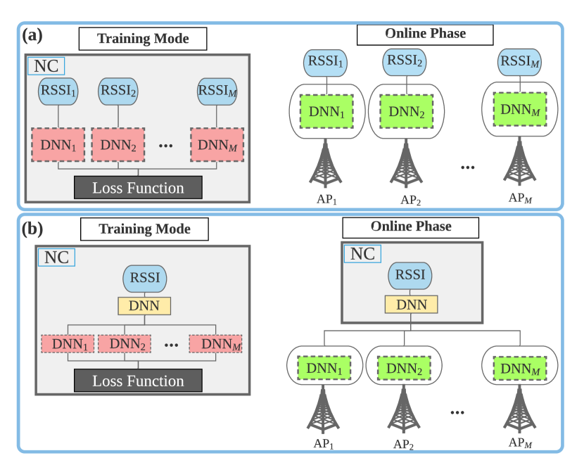
Figure 1: a) fully distributed DNN “FullDeC-HBF” or “FullDeC-FDP”, b) partially distributed DNN “PartDeC-HBF” or “PartDeC-FDP”.

In FullDeC-HBF, a multi-tasking DNN is considered, which jointly performs the regression and classification task to respectively design the DP and the AB. Each local-DNN consists of $2$ convolutional layers (CLs) with $32$ channels, followed by $2$ fully-connected layers (FLs) with $512$ neurons connected to the output layer. Since we use real-valued DNNs, the output layer for the regression task has size $2\times N_{\sf{RF}}\times N_{\sf{U}}$ for each local-DNN. All non-output layers use the “LeakyReLU” activation function and for the output layer of the classifier, the “Softmax” activation function is used to assign a probability to each codewords in the codebook. Hence, we define $\mathbf{p}_{m}=[p_{1,m},...,p_{l,m},...,p_{L_{m},m}]$ as the output of each classifier, where $p_{l,m}$ corresponds to the probability of the $l^{\text{th}}$ codeword in the codebook of the $m^{\text{th}}$ AP and $L_{m}=|\mathcal{A}_{m}|$ is the size of $m^{\text{th}}$ codebook. The size of the classifier in each local-DNN corresponds to the length of the local codebook. For the FDP case, the architecture of FullDeC-FDP is the same as FullDeC-HBF, except for the output layer which only consists of a regression task since there is no AB.

Since we design $M$ parallel local-DNNs, the complexity linearly scales by increasing the number of APs. To address this concern, we propose another architecture in the following based on the auto-encoder concept, enabling lower computational complexity than fully decentralized beamforming.

IV-B Partially Decentralized Beamforming

The second architecture, called “PartDeC-HBF” for HBF or “PartDeC-FDP” for FDP, is shown in Fig 1-(b). Here, we designed the DNN partially distributed with a combination of shared and unshared layers in the training phase. The first idea behind this architecture is to use some shared layers to reduce the total computational complexity both in the training phase and the online phase. To do so, we used $2$ shared CLs with $32$ channels, one FL with $1024$ neurons followed by $M$ parallel groups of unshared layers. Each group consists of $2$ FLs with $200$ and $1024$ neurons. The second idea is to exploit the fact that the combination of the last shared layer with a first unshared layer acts like an auto-encoder, enabling to reduce the signaling overhead. The activation functions are the same as in the fully decentralized case. For the FDP case, PartDeC-FDP is derived from PartDeC-HBF by keeping only the regression task in the output layer.

TABLE I: Comparison of Beamforming Type, Signaling Exchange, and Complexity ($N_{\sf{T}}=64$, $N_{\sf{RF}}=8$, $N_{\sf{U}}=4$, $K=16$, $M=4$)

	Beamforming	# RF chains	Signaling Exchange		# multiplications	Sum-Rate	Architecture
Technique	Type	(per AP)	APs $\to$ NC	NC $\to$ APs	($\times 10^{6})$	(bit/s/Hz)	Type
ZF [5]	FDP (Perfect CSI)	$N_{\sf{T}}$	$2MN_{\sf{T}}N_{\sf{U}}$	$2MN_{\sf{T}}N_{\sf{U}}$	24.4	25.4 (100%)	Centralized
FullDeC-FDP	FDP (RSSI-based)	$N_{\sf{T}}$	0	0	2.9	23.3 (92%)	Decentralized
PartDeC-FDP	FDP (RSSI-based)	$N_{\sf{T}}$	$KMN_{\sf{U}}$	$200M$	1.3	23.2 (92%)	Centralized
CB [5]	FDP (Perfect CSI)	$N_{\sf{T}}$	0	0	0	13.1 (52%)	Decentralized
PE-AltMin [13] + O-FDP	HBF (Perfect CSI)	$N_{\sf{RF}}$	$2MN_{\sf{T}}N_{\sf{U}}$	$2MN_{\sf{RF}}(N_{\sf{T}}+N_{\sf{U}})$	$369.2$	20.2 (100%)	Centralized
PE-AltMin [13] + ZF[5]	HBF (Perfect CSI)	$N_{\sf{RF}}$	$2MN_{\sf{T}}N_{\sf{U}}$	$2MN_{\sf{RF}}(N_{\sf{T}}+N_{\sf{U}})$	$26.2$	19.7 (97%)	Centralized
FullDeC-HBF	HBF (RSSI-based)	$N_{\sf{RF}}$	0	0	2.7	19.5 (96%)	Decentralized
PartDeC-HBF	HBF (RSSI-based)	$N_{\sf{RF}}$	$KMN_{\sf{U}}$	$200M$	1.1	19.4 (96%)	Centralized

IV-C Training Mode

As shown in Fig1-(a), all local-DNNs in FullDeC-HBF or FullDeC-FDP are trained jointly, for instance inside the NC, and all of them are fed with quantized RSSIs obtained from users, as described in Section II. Since we aim to train the DNN with unsupervised learning, we propose the following loss function to train the DNNs for HBF:

$$\mathcal{L}_{\text{HBF}}=-\sum_{l_{1}=1}^{L_{1}}...\sum_{l_{M}=1}^{L_{M}}\Bigg{(}R_{\text{HBF}}(\bar{\mathbf{A}}_{l_{1},...,l_{M}},\bar{\mathbf{W}})\prod_{m=1}^{M}p_{l_{m},m}\Bigg{)},$$ (9)

where $\bar{\mathbf{W}}$ is the DP output of the DNN, $\bar{\mathbf{A}}_{l_{1},...,l_{M}}=\text{diag}(\bar{\mathbf{A}}_{l_{1}},...,\bar{\mathbf{A}}_{l_{M}})$, and $\bar{\mathbf{A}}_{l_{m}}$ is the AB corresponding to the codeword index $l_{m}$. Thus, the loss function is defined in terms of the expected sum rate of the system, given the probabilities assigned to each codeword combination for all local DNNs. Likewise, we define $\mathcal{L}_{\text{FDP}}=-R_{\text{FDP}}(\mathbf{\bar{U}})$ for the FDP where $\mathbf{\bar{U}}$ is the output of the DNN in FullDeC-FDP.

Moreover, batch normalization and dropout are used during training. Finally, to satisfy $\sum_{\forall m}||\bar{\mathbf{A}}_{l_{m}}\bar{\mathbf{w}}_{m}||^{2}=1$, we further normalize $\bar{\mathbf{w}}_{m}$ using the approach proposed in [5] for power allocation. The training phase for PartDeC-HBF or PartDeC-FDP shown in Fig 1-(b) follows the same procedures.

IV-D Online Mode

In the evaluation phase, each AP is assumed to have a local copy of a portion of the DNN (green boxes in Fig. 1). In the case of the fully distributed systems (FullDeC-HBF or FullDeC-FDP), the local DNNs are fully independent, and each AP is able to directly design the precoding as soon as it receives its quantized RSSI feedback. In the case of the partially distributed systems (PartDeC-HBF or PartDeC-FDP), the local DNNs receive inputs from the shared DNN layers (yellow box) in the NC. Consequently, the quantized RSSI input is first processed by the NC, and then the real-valued outputs of the shared DNN are sent from the NC to the APs, which then evaluate the last layers to output the precoding. Note that, although the NC is engaged in the online mode, the signaling overhead is nonetheless reduced compared to a conventional method since the last layer in the NC and the first layer in each AP are sized to form an auto-encoder.

V Simulation Results

In this section, the performance of the four proposed architectures (two for HBF and two for FDP), implemented using the PyTorch DL framework, is evaluated numerically. The deepMIMO channel model [11] is employed to generate the dataset, with parameters $\texttt{active\_BS}=\{4:10\}$, $\texttt{active\_user\_first}=1100$ and $\texttt{active\_user\_last}=2200$. There are $M$ APs ($M\in\{2,4,8\}$), each equipped with $N_{\sf{T}}=64$ antennas and $N_{\sf{RF}}=8$ RF chains with 2-bit phase shifters serving $N_{\sf{U}}=4$ users located randomly. The SSB has size $K=16$, and the RSSI feedback values are quantized on $8$ bits. The size of the DNN dataset is set to $10^{6}$ samples, with $85$% of the samples used for the training set and the remaining ones used to evaluate the performance as test set. The mini-batch size, learning rate and weight decay are set to $1000$, $0.001$, and $10^{-6}$, respectively.

Table I compares the amount of signaling exchange, the computational complexity, and the sum-rate performance of the proposed methods with existing approaches for $\sigma^{2}=-130$ dBW. The top and bottom rows of Table I respectively present results for FDP and HBF techniques. The amount of signaling exchange between the APs and NC is found by counting the number of transferred real matrix coefficients. For the computational complexity, we consider the number of real multiplications (RM) for each matrix multiplication and inversion involved in the algorithms. We assume that one complex multiplication (CM) corresponds to $4$ RMs. General expressions for the number of RMs required by O-FDP and by each DNN layer can be found in [7]. In order to fairly compare the complexity of the fully and partially decentralized alternatives, the DNNs are sized such that the “Full” and “Part” DNNs achieve approximately the same sum rate.

As a near-optimal baseline for HBF, we adapted PE-AltMin [13] for the case of 2-bit phase shifters. For FDP, we compare the proposed solutions with ZF and CB. Since the PE-AltMin method is based on knowing the FDP matrix, Table I considers both a high complexity near-optimal approach (O-FDP) and a low complexity approach (ZF) for obtaining the FDP. The average number of iterations for PE-AltMin to converge is $\ell=18$. Therefore, considering that the singular-value decomposition of an $m\times n$ matrix requires $4m^{2}n+22n^{3}$ RMs [15], the number of RMs for PE-AltMin can be expressed as $\ell M(8N_{\sf{RF}}N_{\sf{U}}(N_{\sf{T}}+N_{\sf{U}})+22N_{\sf{RF}}^{3})$.

When compared to the PE-AltMin + ZF technique, PartDeC-HBF has a slight sum-rate loss of $1$%, but requires $80$% less signaling exchange (uplink + downlink), and is $24\times$ less complex. Moreover, perfect CSI is used for all reference approaches, whereas the proposed DNNs only rely on RSSI measurements as described in Section II. On the other hand, FullDeC-HBF also has a sum-rate loss of $1$%, but requires no signaling exchange while being almost $10\times$ less complex. In comparison to the PE-AltMin + O-FDP, FullDeC-HBF and PartDeC-HBF are respectively $136\times$ and $335\times$ less complex at the cost of a $4$% sum-rate reduction compared to PE-AltMin + O-FDP. Therefore, both proposed DNNs provide near-optimal HBF solutions with significantly less computational complexity and signaling exchange than traditional methods.

As expected, in FDP solution, ZF provides the best FDP sum-rate in high SNR regime. The complexity of ZF is given by $4M^{2}N_{\sf{T}}^{2}(2N_{\sf{U}}+MN_{\sf{T}}/3)$. However, FullDeC-FDP and PartDeC-FDP have almost $8\times$ and $18\times$ lower computational complexity than ZF, respectively, at the cost of $8$% sum-rate loss. For PartDeC-FDP, the signaling exchange between APs and the NC is reduced by $60$% when compared to the ZF solution, while there is no signaling exchange for FullDeC-FDP. CB is the less complex of all techniques and requires no signaling overhead. However, both proposed DNN FDP solutions outperform CB with $77$% higher sum-rate. It is worth noting that the FDP techniques require one RF chain per antenna ($64$ RF chains). Thus, they are not energy efficient compared to HBF techniques which only require $8$ RF chains coupled with 2-bit phase shifters.

In Fig. 2 (a) and (b), we evaluated the achievable sum-rate of the proposed architectures for FDP and HBF, respectively, where in Fig. 2 (a) we compared the FDP solution with ZF [3] and CB [3], and in Fig. 2 (b), the proposed HBF solution has been compared with PE-AltMin as near-optimal solution. We consider different noise power values $\sigma^{2}$ ranging from $-110$ dBW to $-130$ dBW. When considering the channel attenuation, the average signal-to-noise ratios (SNRs) are between $3.1$ dB and $23.1$ dB. It can be seen that the proposed HBF and FDP architectures all provide near-optimal sum-rate performance with decentralized architecture over this noise power range. Among FDP solutions, the CB has poor performance in a high SNR regime because user interference is more dominant. On the other hand, ZF has poor performance in the low SNR regime and a low number of APs. Finally, Fig. 3 shows the cumulative distribution function (CDF) of the per-user rates. It is shown that both proposed DNN architectures focus on maximizing the average sum-rate and neglect users with worse channels. This is expected since no notion of fairness has been included in the loss function used to train the DNNs.

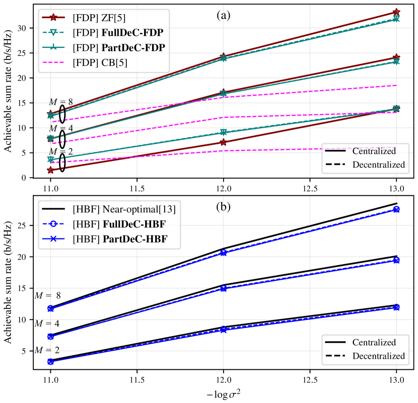
Figure 2: Achievable sum-rate (b/s/Hz) performance (a) FDP, (b) HBF.

VI Conclusion

CF-mMIMO is a promising technique to increase the throughput and improve the coverage, but conventional approaches for designing the precoder at each AP are complex and require a significant communication overhead, both in the case of FDP and HBF architectures. In this paper, we proposed two RSSI-based DNNs with distributed architectures to design a coordinated FDP or HBF precoder. The experimental results on a millimeter-wave ray-tracing model show that the proposed DNNs can achieve near optimal performance for both FDP and HBF systems, while significantly reducing the computational complexity and the signaling overhead. Furthermore, the signaling overhead can be completely eliminated at the cost of increased complexity.

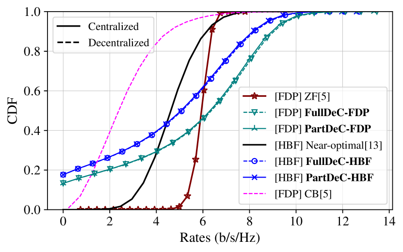
Figure 3: CDFs of the per-user rates ($\sigma^{2}=-130$, $M=4$, $N_{\sf{T}}=64$).

References

- [1] T. L. Marzetta, “Noncooperative cellular wireless with unlimited numbers of base station antennas,” IEEE Transactions on Wireless Communications, vol. 9, no. 11, pp. 3590–3600, 2010.
- [2] H. Q. Ngo, A. Ashikhmin, H. Yang, E. G. Larsson, and T. L. Marzetta, “Cell-Free Massive MIMO Versus Small Cells,” IEEE Trans. Wireless Commun., vol. 16, no. 3, pp. 1834–1850, 2017.
- [3] H. Yang and T. L. Marzetta, “Energy Efficiency of Massive MIMO: Cell-Free vs. Cellular,” in 2018 IEEE Vehic. Tech. Conf., 2018, pp. 1–5.
- [4] E. Björnson and L. Sanguinetti, “Making Cell-Free Massive MIMO Competitive With MMSE Processing and Centralized Implementation,” IEEE Trans. Wireless Commun., vol. 19, no. 1, pp. 77–90, 2020.
- [5] E. Nayebi, A. Ashikhmin, T. L. Marzetta, H. Yang, and B. D. Rao, “Precoding and Power Optimization in Cell-Free Massive MIMO Systems,” IEEE Trans. Wireless Commun., vol. 16, no. 7, pp. 4445–4459, 2017.
- [6] A. F. Molisch, V. V. Ratnam, S. Han, Z. Li, S. L. H. Nguyen, L. Li, and K. Haneda, “Hybrid Beamforming for Massive MIMO: A Survey,” IEEE Commun. Mag., vol. 55, no. 9, pp. 134–141, 2017.
- [7] H. Hojatian, J. Nadal, J.-F. Frigon, and F. Leduc-Primeau, “Unsupervised Deep Learning for Massive MIMO Hybrid Beamforming,” IEEE Trans. Wireless Commun., pp. 1–1, 2021.
- [8] H. Huang, Y. Song, J. Yang, G. Gui, and F. Adachi, “Deep-Learning-Based Millimeter-Wave Massive MIMO for Hybrid Precoding,” IEEE Trans. on Veh. Technol., vol. 68, no. 3, pp. 3027–3032, 2019.
- [9] A. Alkhateeb, S. Alex, P. Varkey, Y. Li, Q. Qu, and D. Tujkovic, “Deep learning coordinated beamforming for Highly-Mobile millimeter wave systems,” IEEE Access, vol. 6, pp. 37 328–37 348, 2018.
- [10] B. Lee, J. Choi, J.-Y. Seol, D. J. Love, and B. Shim, “Antenna Grouping Based Feedback Compression for FDD-Based Massive MIMO Systems,” IEEE Trans. Commun., vol. 63, no. 9, pp. 3261–3274, 2015.
- [11] A. Alkhateeb, “DeepMIMO: A Generic Deep Learning Dataset for Millimeter Wave and Massive MIMO Applications,” in Proc. Inf. Theory and App. Workshop (ITA), San Diego, CA, 2019, pp. 1–8.
- [12] H. Hojatian, V. N. Ha, J. Nadal, J.-F. Frigon, and F. Leduc-Primeau, “RSSI-Based Hybrid Beamforming Design with Deep Learning,” in ICC 2020 - IEEE Int. Conf. Commun. (ICC), Jun 2020, pp. 1–6.
- [13] X. Yu, J. Shen, J. Zhang, and K. B. Letaief, “Alternating Minimization Algorithms for Hybrid Precoding in Millimeter Wave MIMO Systems,” IEEE J. Sel. Topics in Signal Proc., vol. 10, no. 3, pp. 485–500, 2016.
- [14] E. Bjornson, M. Bengtsson, and B. Ottersten, “Optimal multiuser transmit beamforming: A difficult problem with a simple solution structure,” IEEE Sig. Proc. Mag., vol. 31, no. 4, pp. 142–148, 2014.
- [15] V. L. Golub, Matrix Computations. Johns Hopkins University Press, Mar. 1996.