Resilient UAV Swarm Communications with Graph Convolutional Neural Network

Abstract

In this paper, we study the self-healing problem of unmanned aerial vehicle (UAV) swarm network (USNET) that is required to quickly rebuild the communication connectivity under unpredictable external destructions (UEDs). Firstly, to cope with the one-off UEDs, we propose a graph convolutional neural network (GCN) that can find the recovery topology of the USNET in an on-line manner. Secondly, to cope with general UEDs, we develop a GCN based trajectory planning algorithm that can make UAVs rebuild the communication connectivity during the self-healing process. We also design a meta learning scheme to facilitate the on-line executions of the GCN. Numerical results show that the proposed algorithms can rebuild the communication connectivity of the USNET more quickly than the existing algorithms under both one-off UEDs and general UEDs. The simulation results also show that the meta learning scheme can not only enhance the performance of the GCN but also reduce the time complexity of the on-line executions.

I Introduction

Unmanned aerial vehicle (UAV) swarm network (USNET) that contains hundreds or even thousands UAVs usually works in open, sometimes even harsh environments and is susceptible to external disruptions [1]. Since the failure of any part of UAVs could be a fatal blow to the entire USNET, the resilient USNETs with the self-healing capacity are urgently demanded in various applications, such as data collections [2, 3], rescue [4], security and surveillance [5, 6], etc. Researchers have studied the self-healing mechanisms for USNETs in multiple tasks. For example, the authors of [7] developed a real-time resilient method based on the communication connectivity of multi-UAV systems. The authors of [8] proposed an intrusion detection scheme based on data exchanging through communication connections to improve the security resilience of the UAV network. Moreover, the authors of [9] developed the resilient algorithms for localization, gathering, and network configurations that highly depend on the communication connectivity of the USNET. Obviously, the communication connectivity plays an important role in different kinds of self-healing mechanisms, and thus the self-healing of the communication connectivity (SCC) becomes a basic requirement for various resilient USNETs.

Many algorithms have been developed to deal with the SCC problem for the wireless sensor networks (WSNs) [11, 12, 13, 14, 15, 16, 17, 18, 19, 20, 21], and were later extended to the USNETs [22, 23]. However, there still remain several challenges to the SCC problem in USNET. Firstly, many existing algorithms [12, 13, 14, 16, 17, 21] are heuristic and may not be able to guarantee the communication connectivity of the USNET. For example, these algorithms could not work when the number of UAVs is large, especially under massive destructions. Other algorithms [15, 18, 19, 20, 23, 22] could make sure that the UAVs rebuild the communication connectivity but at the cost of lots of resources, such as self-healing time and communication overheads. The second challenge lies in the high time complexities during real-time executions. It is worth noting that the real-time execution time complexity is an important indicator to evaluate the resilience of the USNET, since it relates to the self-healing time and even the degree of destructions [24]. For example, the algorithm in [11] needs to find the global cut vertexes of the WSN during the self-healing process, which makes its on-line execution time complexity increase with the size of the WSN. The algorithm in [19] needs to calculate the optimal critical sensors for WSNs during on-line executions, which may consume a lot of time.

The third challenge is the difficulty in dealing with complex destructions. The external destructions can be divided into predictable external destructions (PEDs) and unpredictable external destructions (UEDs). PEDs can be mitigated or even avoided by finding the pattern of destructions, while UEDs could have serious impacts on the USNETs and should be carefully handled [1]. UEDs can be further divided into one-off UEDs and general UEDs. One-off UEDs happen only once and can destruct a random number of UAVs simultaneously. Almost all the existing UED algorithms [11, 12, 13, 14, 15, 16, 17, 18, 19, 20, 21, 22, 23] are proposed for one-off UEDs. Moreover, many of the UED algorithms [11, 12, 14, 16, 17] were designed regarding to the failure of only one UAV in one-off UEDs, which is relatively basic and simple. Other UED algorithms [13, 18, 15] were developed for the failure of multiple UAVs in one-off UEDs, but exclusively focused on the scenarios where a small number of UAVs were destructed. In fact, a general UED can destruct any number of UAVs at random time steps, which is more common in practice but more difficult to handle. However, to the best of our knowledge, the general UEDs have not been considered in literatures, yet.

In this paper, we study the SCC problem of the USNET under two types of UEDs, separately. To cope with one-off UEDs, we propose a graph convolutional operation (GCO) that can theoretically guarantee the SCC of the USNET. We then extend the GCO to a graph convolutional neural network (GCN) to minimize the SCC time of the USNET. Moreover, we design a meta learning scheme for the GCN to reduce the time complexity of on-line executions. To cope with general UEDs, we develop a monitoring mechanism that can detect UEDs for UAVs and design a self-healing trajectory planning algorithm based on the GCN and the monitoring mechanism. The numerical results show that the proposed algorithms can rebuild the communication connectivity of the USNET much faster than the existing algorithms under both one-off and general UEDs. The simulation results also show that the meta learning scheme can make the GCN converge faster and reduce the time of on-line executions under both types of UEDs.

TABLE I: The Summarization of Abbreviations

Abbreviations	Full Name	Abbreviations	Full Name
UAV	unmanned aerial vehicle	USNET	unmanned aerial vehicle swarm network
SCC	self-healing of the communication connectivity	WSN	wireless sensor network
PED	predictable external destruction	UED	unpredictable external destruction
GCO	graph convolutional operation	GCN	graph convolutional network
CCN	connected communication network	MCL	multi-hop of communication link
RUAV	remaining UAV	A2A	air-to-air
CLEC	communication link establish condition	FT	Fourier transform
CR-MGC	communication-relaxed meta graph convolution (dealing with one-off UEDs)	VRG	virtual RUAV graph
GCL	graph convolutional layer	mGCN	meta GCN
IDB	individual data base	IISR	individual index set of RUAVs
CR-MGCM	communication-relaxed meta graph convolution method (dealing with general UEDs using monitoring mechanisms)	CR-MGCMglob	communication-relaxed meta graph convolution method (dealing with general UEDs using global information)

The rest parts of this paper are organized as follows. Section II presents the system models of the SCC problem for USNET. Section III describes the proposed GCN and meta learning scheme under one-off UEDs. Section IV focuses on the monitoring mechanisms and trajectory planning algorithm of UAVs under the general UEDs. Simulation results and analysis are provided in Section V, and conclusions are made in Section VI. The abbreviations are summarized in Table I.

Notations: $x$, $\mathbf{x}$, $\mathbf{X}$ represent a scalar $x$, a vector $\mathbf{x}$ and a matrix $\mathbf{X}$, respectively; $\sum$, $\min$, $\max$ and $\nabla$ denote the sum, minimum, maximum and vector differential operator, respectively; $(x_{ij})$ represents a matrix with element $x_{ij}$ in the $i$-th row and the $j$-th column, and $(\mathbf{X})_{ij}$ represents the element of row $i$ and column $j$ in matrix $\mathbf{X}$; $\left\|\cdot\right\|_{2}$ and $\left\|\cdot\right\|_{\infty}$ denote the 2-norm and infinite norm of matrices, respectively; $\cup$, $\cap$ and $\backslash$ represent the union operator, the intersection operator and the difference operator between sets; $|\mathcal{S}|$ represents the number of elements in set $\mathcal{S}$; $\mathbb{R}^{N\times M}$, $\mathbb{S}^{N}$ and $\mathbb{S}^{N}_{+}$ represent the $N$-by-$M$ real matrix space, the $N$-by-$N$ symmetric matrix space and the $N$-by-$N$ positive semi-definite matrix space; $\mathbb{N}_{+}$ represents the set of positive integers; $\mathbf{1}_{n}$ represents an $n$-dimensional vector where the components are all $1$’s; $\mathbbm{1}\{\cdot\}$ represents the indicative function with range $\{0,1\}$, $\leftarrow$ denotes the assignment from right to left, while $\rightarrow$ represents the approximation of the right term by the left term; $\triangleq$ defines the symbol on the left by the equation on the right.

II System Model

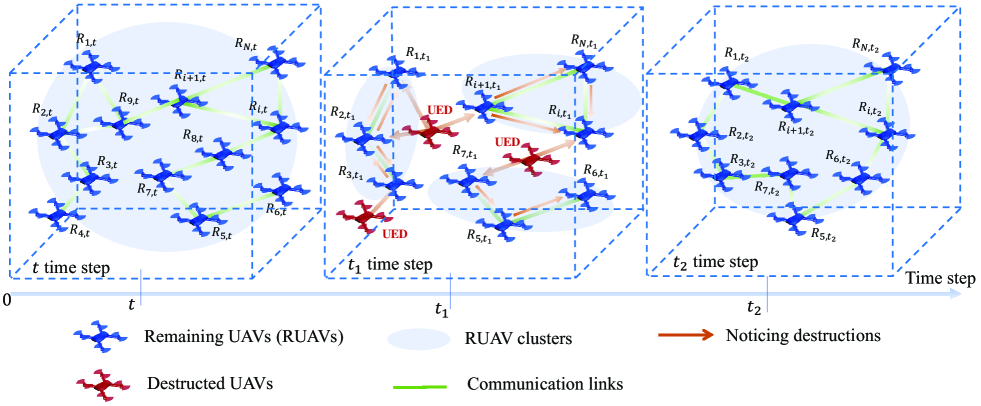
Figure 1: The USNET rebuild its communication connectivity under UEDs.

We consider a USNET with $N$ identical UAVs, where each UAV is endowed with a fixed index $i\in\mathcal{N}\triangleq\{1,2,...,N\}$, as shown in Fig. 1. Establish an $X$-$Y$-$Z$ Cartesian coordinate for the USNET, and let the position of the $i$-th UAV at time step $t$ be $\mathbf{p}_{i,t}=[x_{i,t},y_{i,t},z_{i,t}]^{T},\;i\in\mathcal{N}$, where $x_{i,t}$, $y_{i,t}$ and $z_{i,t}$ represent the $X$, $Y$ and $Z$ axis components, respectively. Each UAV can transmit signals to other UAVs with constant power $P$. The $i$-th and the $i^{\prime}$-th UAVs can establish a communication link $e_{ii^{\prime},t}$ (or $e_{i^{\prime}i,t}$) at time step $t$ when the powers of the signals received by the $i$-th and the $i^{\prime}$-th UAV from each other, denoted as $P_{b}(i,i^{\prime})$ and $P_{b}(i^{\prime},i)$, both exceed a threshold $P_{0}$, i.e.,

$$P_{b}(i,i^{\prime})\geq P_{0}\;\;\text{and}\;\;P_{b}(i^{\prime},i)\geq P_{0}.$$ (1)

Any two UAVs with a valid communication link are marked as neighbors of each other. The initial USNET forms a connected communication network (CCN), where each UAV can transmit data to any other UAVs in the USNET through multi-hop of communication links (MCLs).

Due to the hash environments, the UEDs can destruct random UAVs at any time step and thus destroy the CCN. The destructed UAVs are forced to detach from the USNET, which can be sensed by their neighbors. The remaining UAVs (RUAVs) react against the destructions and try to restore the CCN by adjusting their positions. Once RUAVs rebuild CCN, they stop flying immediately to avoid gathering denser such that the impact of the next UEDs can be reduced. We denote the index set of RUAVs at time step $t$ as $\mathcal{I}_{t}\triangleq\{i|\text{the }i\text{-th UAV remains at time step }t,i\in\mathcal{N}\}$. Let us sort the elements in $\mathcal{I}_{t}$ in an ascending order, and re-represent it as $\mathcal{I}_{t}=\{r_{1},r_{2},...,r_{|\mathcal{I}_{t}|}\}$, where $r_{j}$ represents the $j$-th smallest element in $\mathcal{I}_{t}$, or equivalently, the $j$-th smallest index among all RUAVs, $j\in\{1,2,...,|\mathcal{I}_{t}|\}$. Denote the RUAV with index $i$ at time step $t$ as RUAV_i,t, and then the set of RUAVs at time step $t$ can be defined as $\mathcal{R}_{t}\triangleq\{\text{RUAV}_{i,t}|i\in\mathcal{I}_{t}\}=\{\text{RUAV}_{r_{1},t},\text{RUAV}_{r_{2},t},...,\text{RUAV}_{r_{|\mathcal{I}_{t}|},t}\}$. Assume the magnitude of the flying speed of each UAV is a constant $v_{0}>0$. The speed of RUAV_i,t at time step $t$ can thus be represented as $\mathbf{v}_{i,t}=\check{\mathbf{v}}_{i,t}v$, where $\check{\mathbf{v}}_{i,t}$ is the unit vector of the flying direction, i.e., $\left\|\check{\mathbf{v}}_{i,t}\right\|_{2}=1$, and $v\in\{v_{0},0\}$.

II-A Communication Link Between UAVs

We model the communication channels between UAVs as air-to-air (A2A) communication links [30, 31]. At each time step $t$, the power of the received signals of the $i$-th UAV from the $i^{\prime}$-th UAV is calculated as

$$P_{b}(i,i^{\prime})=P+G_{1}+G_{2}-L(\mathbf{p}_{i,t},\mathbf{p}_{i^{\prime},t})-p_{\xi}(\mathbf{p}_{i,t},\mathbf{p}_{i^{\prime},t}),$$ (2)

where $G_{1}$ and $G_{2}$ represent the constant antenna gains of the receiving and transmitting UAVs, respectively, $L(\mathbf{p}_{i,t},\mathbf{p}_{i^{\prime},t})$ is the large-scale fading effect, and $p_{\xi}(\mathbf{p}_{i,t},\mathbf{p}_{i^{\prime},t})$ is the small-scale fading effect. Since there is no ground obstacle for USNET, the large-scale effect $L(\mathbf{p}_{i,t},\mathbf{p}_{i^{\prime},t})$ can be expressed as

$$L(\mathbf{p}_{i,t},\mathbf{p}_{i^{\prime},t})=10\alpha\log_{10}\bigg{(}\frac{4\pi\left\|\mathbf{p}_{i,t}-\mathbf{p}_{i^{\prime},t}\right\|_{2}f_{c}}{v_{c}}\bigg{)},$$ (3)

where $\alpha>0$ is the path loss exponent, $f_{c}$ is the electromagnetic wave frequency, and $v_{c}$ is the speed of light. The small-scale fading effect $p_{\xi}(\mathbf{p}_{i,t},\mathbf{p}_{i^{\prime},t})$ is usually modeled as the Rice function [32], i.e.,

$$p_{\xi}(\mathbf{p}_{i,t},\mathbf{p}_{i^{\prime},t}) =\frac{\left\|\mathbf{p}_{i,t}-\mathbf{p}_{i^{\prime},t}\right\|_{2}}{\sigma_{0}^{2}}\exp\bigg{(}\frac{-\left\|\mathbf{p}_{i,t}-\mathbf{p}_{i^{\prime},t}\right\|_{2}^{2}-\rho^{2}}{2\sigma_{0}^{2}}\bigg{)}$$

$$I_{0}(2K\left\|\mathbf{p}_{i,t}-\mathbf{p}_{i^{\prime},t}\right\|_{2}),$$ (4)

where $\rho$ and $\sigma_{0}$ represent the strength of the dominant and scattered (non-dominant) paths, respectively, $I_{0}$ is the $0$-th order modified Bessel function of the first kind, and $K=\frac{\rho^{2}}{2\sigma_{0}^{2}}$ is the Rice factor. Since the received signal power $P_{b}(i,i^{\prime})$ only relates to the relative distance between the $i$-th and the $i^{\prime}$-th UAVs, i.e., $l_{ii^{\prime},t}=l_{i^{\prime}i,t}\triangleq\left\|\mathbf{p}_{i,t}-\mathbf{p}_{i^{\prime},t}\right\|_{2}$, the received signal power $P_{b}(i^{\prime},i)$ equals to $P_{b}(i,i^{\prime})$, i.e.,

$$P_{b}(i^{\prime},i)=P_{b}(i,i^{\prime}).$$ (5)

From (1), (2), (3), (II-A) and (5), we know that any two distinct UAVs with index $i$ and $i^{\prime}$ can establish a communication link if their distance $l_{ii^{\prime},t}$ satisfies:

$$10\alpha \log_{10}\bigg{(}\frac{4\pi l_{ii^{\prime},t}f_{c}}{v_{c}}\bigg{)}+\frac{l_{ii^{\prime},t}}{\sigma_{0}^{2}}\exp\bigg{(}\frac{-l_{ii^{\prime},t}^{2}-\rho^{2}}{2\sigma_{0}^{2}}\bigg{)}I_{0}(2Kl_{ii^{\prime},t})$$

$$\leq P+G_{1}+G_{2}-P_{0}.$$ (6)

Equation (II-A) is called as the communication link establish condition (CLEC).

II-B RUAV Graph

RUAVs at each time step $t$ can be viewed as an undirected graph $\mathcal{G}_{t}=\{\mathcal{R}_{t},\mathcal{E}_{t},\mathbf{X}_{t}\}$ [23], named as RUAV graph, where $\mathcal{R}_{t}$ acts as the node set, and $\mathcal{E}_{t}=\{e_{ii^{\prime},t}|i,i^{\prime}\in\mathcal{I}_{t}\}$ is the edge set containing all the communication links of RUAVs. The third term $\mathbf{X}_{t}\in\mathbb{R}^{|\mathcal{I}_{t}|\times 3}$ is the topology matrix that concatenates the positions of RUAVs, i.e., $\mathbf{X}_{t}=[\mathbf{p}_{r_{1},t},\mathbf{p}_{r_{2},t},...,\mathbf{p}_{r_{|\mathcal{I}_{t}|},t}]^{T}$. We define an RUAV cluster as a subset of $\mathcal{R}_{t}$, where RUAVs in an RUAV cluster form a local CCN but with no communication links to other RUAV clusters. Denote $C_{t}\in\mathbb{N}_{+}$ as the number of RUAV clusters at time step $t$. Due to the UEDs, the RUAV graph $\mathcal{G}_{t}$ contains at least one RUAV cluster at each time step $t$, i.e., $C_{t}\geq 1$. For example, as shown in Fig. 1, the RUAV graph $\mathcal{G}_{t}$ has $3$ RUAV clusters at time step $t_{1}$, while emerges to one RUAV cluster and forms a CCN at time step $t_{2}$.

Define the adjacency matrix of the RUAV graph $\mathcal{G}_{t}$ as $\mathbf{A}_{t}=(a_{jj^{\prime},t})\in\mathbb{S}^{|\mathcal{I}_{t}|}$, where $a_{jj^{\prime},t}\in\{0,1\},j,j^{\prime}\in\{1,2,...,|\mathcal{I}_{t}|\}$. Note that if $j\neq j^{\prime}$ and the communication link $e_{r_{j}r_{j^{\prime}},t}$ exists between RUAV${}_{r_{j},t}$ and RUAV${}_{r_{j^{\prime}},t}$, then $a_{jj^{\prime},t}=a_{j^{\prime}j,t}=1$; otherwise $a_{jj^{\prime},t}=a_{j^{\prime}j,t}=0$. The degree matrix of the RUAV graph $\mathcal{G}_{t}$ is defined as a diagonal matrix $\mathbf{D}_{t}=\text{diag}(d_{1,t},d_{2,t},...,d_{{|\mathcal{I}_{t}|},t})\in\mathbb{S}^{|\mathcal{I}_{t}|}$,where $d_{j,t}=\sum_{j^{\prime}=1}^{|\mathcal{I}_{t}|}a_{jj^{\prime},t}$ is the number of the neighbors of RUAV${}_{r_{j},t}$. The Laplace matrix of the RUAV graph $\mathcal{G}_{t}$ is defined as the difference between $\mathbf{D}_{t}$ and $\mathbf{A}_{t}$, i.e.,

$$\mathbf{L}_{t}=\mathbf{D}_{t}-\mathbf{A}_{t}.$$ (7)

As the Laplace matrix $\mathbf{L}_{t}$ is a positive semi-definite matrix [33], we can perform eigenvalue decomposition,

$$\mathbf{L}_{t}=\mathbf{U}_{t}\mathbf{\Lambda}_{t}\mathbf{U}^{T}_{t},$$ (8)

where $\mathbf{U}_{t}=[\mathbf{u}_{1,t},\mathbf{u}_{2,t},...,\mathbf{u}_{|\mathcal{I}_{t}|,t}]$ is a unitary matrix composed of $|\mathcal{I}_{t}|$ mutually orthogonal eigenvectors, and $\mathbf{\Lambda}_{t}=\text{diag}(\lambda_{1,t},\lambda_{2,t},...,\lambda_{|\mathcal{I}_{t}|,t})$ is a diagonal matrix with non-negative eigenvalues. Notice that 0 must be one of the eigenvalues of $\mathbf{L}_{t}$, since

$$\mathbf{L}_{t}\mathbf{1}_{|\mathcal{I}_{t}|} =(\mathbf{D}_{t}-\mathbf{A}_{t})\mathbf{1}_{|\mathcal{I}_{t}|}=\begin{pmatrix}d_{1,t}-\sum_{j=1}^{|\mathcal{I}_{t}|}a_{1j,t}\\ \vdots\\ d_{{|\mathcal{I}_{t}|},t}-\sum_{j=1}^{|\mathcal{I}_{t}|}a_{{|\mathcal{I}_{t}|}j,t}\end{pmatrix}$$

$$=\mathbf{0}=0\mathbf{1}_{|\mathcal{I}_{t}|},$$ (9)

and $\mathbf{1}_{|\mathcal{I}_{t}|}$ is one possible corresponding eigenvector. The algebraic multiplicity of the zero eigenvalue $\Omega(\lambda=0|\mathbf{L}_{t})$ equals to the number of RUAV clusters $C_{t}$ of the RUAV set $\mathcal{R}_{t}$ at each time step $t$, i.e., $\Omega(\lambda=0|\mathbf{L}_{t})=C_{t}$ [33]. Hence, if $\Omega(\lambda=0|\mathbf{L}_{t})=C_{t}=1$, then RUAVs form a CCN, while if $\Omega(\lambda=0|\mathbf{L}_{t})=C_{t}>1$ otherwise.

II-C Problem Formulation

The goal of the SCC problem of resilient USNET is that RUAVs should try to reform CCNs as quickly as possible after UEDs. We first study the SCC problem under one-off UEDs, where the initial USNET is destructed by a random UED only once at time step $t$ and self-heal afterwards. For a USNET with $N$ UAVs, there are $2^{N}$ cases of one-off UEDs, where different cases of one-off UEDs destruct different number of UAVs with different indexes. Note that not all cases of one-off UEDs can destroy the communication connectivity of the USNET, and we only consider the one-off UEDs that can break up the USNET into more than one RUAV clusters (see Appendix A). Denote the flying time of RUAV_i,t during the self-healing process as $\phi[i]$. Then the total self-healing time steps can be expressed as $\max_{i\in\mathcal{I}_{t}}\phi[i]$. Since RUAV_i,t should fly in a straight line to reduce $\phi[i]$ and since the magnitude of the flying speed is a constant $v_{0}$, the self-healing time steps $\phi[i]$ is proportional to the flying distance of RUAV_i,t. Hence, the SCC problem under one-off UEDs is equivalent to finding a topology matrix $\widetilde{\mathbf{{X}}}_{t}=[\widetilde{\mathbf{p}}_{r_{1},t},\widetilde{\mathbf{p}}_{r_{2},t},...,\widetilde{\mathbf{p}}_{r_{|\mathcal{I}_{r,0}|},t}]^{T}$ that can minimize the largest displacement among all RUAVs, i.e.,

$$(\mathbf{P1}):\;\min_{\widetilde{\mathbf{X}}_{t}}\quad J_{s}=\max_{i\in\mathcal{I}_{t}}v_{0}\phi[i]=\max_{i\in\mathcal{I}_{t}}\left\|\widetilde{\mathbf{p}}_{i,t}-\mathbf{p}_{i,t}\right\|_{2}$$ (10)

$$\operatorname{s.t.}\quad \widetilde{\mathcal{G}}_{t}=\{\mathcal{R}_{t},\widetilde{\mathcal{E}}_{t},\widetilde{\mathbf{X}}_{t}\}\text{ forms a CCN under CLEC},$$ (10a)

where $\mathbf{p}_{i,t}=\mathbf{p}_{i,0}$, and $\widetilde{\mathcal{E}}_{t}\triangleq\{e_{ii^{\prime},t}|\widetilde{l}_{ii^{\prime},t}=\left\|\widetilde{\mathbf{p}}_{i,t}-\widetilde{\mathbf{p}}_{i^{\prime},t}\right\|_{2}\text{satisfies CLEC},\forall i\neq i^{\prime},i,i^{\prime}\in\mathcal{I}_{t}\}$.

We next study the SCC problem under the general UEDs, where the USNET needs to quickly rebuild its communication connectivity under the general UEDs. Under the circumstances, RUAVs can only obtain partial information from each other and need to adjust their flying directions continuously during the self-healing process. We consider a period of $T$ time steps. Define the connected time step ratio $J_{c}=\frac{1}{T}\sum_{t=1}^{T}\mathbbm{1}\{C_{t}=1\}$ as the ratio between the number of time steps when the USNET forms a CCN and the total time steps $T$. Let $J_{c}$ be the performance indicator of the USNET. Then the SCC problem under the general UEDs can be formulated as a functional optimization problem

$$(\mathbf{P2}):\; \mathop{\rm{max}}_{{\mathbf{v}}_{1,t},{\mathbf{v}}_{2,t},...,{\mathbf{v}}_{N,t}\atop t\in\{1,2,...,T\}}\quad J_{c}=\frac{1}{T}\sum_{t=1}^{T}\mathbbm{1}\{C_{t}=1\}$$ (11)

$$\operatorname{s.t.}\;\; \mathbf{p}_{i,t}=\mathbf{p}_{i,t-1}+{\mathbf{v}}_{i,t},\;\forall i\in\mathcal{I}_{t},t\in\{1,2,...,T\}$$ (11a)

$$\mathcal{I}_{T}\subseteq\mathcal{I}_{T-1}\subseteq...\subseteq\mathcal{I}_{0},$$ (11c)

$$(\ref{CL}),$$ (11d)

where (11a) is the dynamic model of RUAVs, (11c) represents the general UEDs to the USNET, and (11d) is the CLEC.

III SCC Algorithm for One-off UEDs

Let us consider the SCC problem under one-off UEDs $(\mathbf{P1})$. Inspired from the existing swarm algorithms [34, 35], one RUAV should pay more attention on the positions of its neighbors during the self-healing process. Since graph neural networks (GNNs) [25, 26, 27, 28] can efficiently gather the neighbor information for each RUAV, we develop a GNN-based algorithm for $(\mathbf{P1})$.

Analogous to the Fourier transform (FT) in the time domain, we can define the FT of the RUAV graph $\mathcal{G}_{t}$ by the eigen-decomposition of the Laplace matrix $\mathbf{L}_{t}$ in (8), where the eigenvectors $\mathbf{u}_{j,t}$ denote the Fourier modes and the eigenvalues $\lambda_{j,t}$ denote the frequency of the RUAV graph $\mathcal{G}_{t}$ [28]. Regarding the topology matrix $\mathbf{X}_{t}$ as a signal of the RUAV graph $\mathcal{G}_{t}$, we can define the FT of $\mathbf{X}_{t}$ as $\breve{\mathbf{X}}_{t}=\mathbf{U}^{T}_{t}\mathbf{X}_{t}$. Hence, the GCO between $\mathbf{X}_{t}$ and the convolutional kernel $\mathbf{g}\in\mathbb{R}^{|\mathcal{I}_{t}|\times 3}$ can be expressed as [36]

$$\mathbf{g}\circ\mathbf{X}_{t}=\mathbf{U}_{t}[(\mathbf{U}^{T}_{t}\mathbf{g})\odot(\mathbf{U}^{T}_{t}\mathbf{X}_{t})],$$ (12)

where $\circ$ represents the convolutional operator, and $\odot$ is the Hadamard product. To decrease the computation complexity of the convolutional kernel, we approximate (12) by truncated Chebyshev polynomials of the first class [27], and the GCO can be expressed as

$$\mathbf{U}_{t}[(\mathbf{U}^{T}_{t}\mathbf{g})\odot(\mathbf{U}^{T}_{t}\mathbf{X}_{t})] =\mathbf{U}_{t}\bigg{(}\sum_{s=0}^{1}\theta_{s}F_{s}({\mathbf{\Delta}}_{t})\bigg{)}\mathbf{U}_{t}\mathbf{X}_{t}$$

$$=\theta_{0}\mathbf{X}_{t}+\theta_{1}(\mathbf{L}_{t}-\mathbf{I}_{t})\mathbf{X}_{t},$$ (13)

where $F_{s}$ represents the $s$-th term in the Chebyshev polynomials, $\mathbf{I}_{t}\in\mathbb{S}^{|\mathcal{R}_{t}|}$ is the identity matrix, $\theta_{0}$ and $\theta_{1}$ are two constant parameters, and ${\mathbf{\Delta}}_{t}=\frac{2\mathbf{\Lambda}_{t}}{\mathbf{\lambda}_{1,t}}-\mathbf{I}_{t}$. Particularly, we define a hyperparameter $H_{t}\triangleq-\theta_{1}>0$ and let $\theta_{0}-\theta_{1}=1$. Then we can define a GCO on the RUAV graph $\mathcal{G}_{t}$ as

$$\mathbf{g}\circ\mathbf{X}_{t}=(\mathbf{I}_{t}-H_{t}\mathbf{L}_{t})\mathbf{X}_{t}.$$ (14)

Based on (14), we propose a communication-relaxed meta graph convolution (CR-MGC) algorithm for the SCC problem under one-off UEDs $(\mathbf{P1})$. The CR-MGC includes the virtual communication relaxing part and the meta graph convolutional network part, as will be stated as follows.

III-A Virtual Communication Relaxing

After UED at time step $t$, the RUAV graph $\mathcal{G}_{t}$ cannot form a CCN under the CLEC (II-A). Nevertheless, we here build a virtual RUAV graph (VRG), denoted as $\mathcal{G}^{v}_{t}=\{\mathcal{R}^{v}_{t},\mathcal{E}^{v}_{t},\mathbf{X}^{v}_{t}\}$, that has the same node set and topology matrix with the RUAV graph $\mathcal{G}_{t}$, but has the different edge set, i.e., $\mathcal{R}^{v}_{t}=\mathcal{R}_{t}$, $\mathbf{X}^{v}_{t}=\mathbf{X}_{t}$, but $\mathcal{E}^{v}_{t}\neq\mathcal{E}_{t}$. We want the VRG to form a CCN. To this end, we design the edge set as $\mathcal{E}^{v}_{t}=\{e^{v}_{ii^{\prime},t}|l_{ii^{\prime},t}\leq d_{t}^{v},\forall i\neq i^{\prime},i,i^{\prime}\in\mathcal{I}_{t}\}$, where $d_{t}^{v}>0$ is a hyperparameter, named as the virtual distance. This indicates that any two distinct RUAV_i,t and RUAV${}_{i^{\prime},t}$ can establish a communication link $e^{v}_{ii^{\prime},t}$ in the VRG if their distance is within the range of $d_{t}^{v}$. Since the VRG is expected to form a CCN, the virtual distance $d_{t}^{v}$ should be large enough to make RUAVs establish sufficient communication links in the VRG. Obviously, there must exist a minimum threshold $d_{min,t}^{v}$ that can just guarantee the VRG to form a CCN. We propose an algorithm to find such $d_{min,t}^{v}$ in Algorithm 1.

Algorithm 1 Find the Minimum Threshold $d_{min,t}^{v}$ for the Virtual Distance $d_{t}^{v}$

Inputs: The topology matrix $\mathbf{X}_{t}$, the index set of RUAVs $\mathcal{I}_{t}$.
Outputs: The minimum threshold $d_{min,t}^{v}$.
Initialize: An empty set $\mathcal{M}_{t}$ to store the pair-wise distance.

1:Calculate the distance between each pair of RUAVs and store them in $\mathcal{M}_{t}$, i.e., $\mathcal{M}_{t}=\{\left\|\mathbf{p}_{i,t}-\mathbf{p}_{i^{\prime},t}\right\|_{2}\;|\;\forall i\neq i^{\prime},i,i^{\prime}\in\mathcal{I}_{t}\}$, the size of $\mathcal{M}_{t}$ is $|\mathcal{M}_{t}|=\frac{|\mathcal{I}_{t}|(|\mathcal{I}_{t}|-1)}{2}$;

2:Sort the elements in $\mathcal{M}_{t}$ in ascending order, i.e., $\mathcal{M}_{t}=\{m_{\zeta,t}|\zeta\in\{1,2,...,\frac{|\mathcal{I}_{t}|(|\mathcal{I}_{t}|-1)}{2}\}\}$, where $m_{1,t}\leq m_{2,t}\leq...\leq m_{\frac{|\mathcal{I}_{t}|(|\mathcal{I}_{t}|-1)}{2},t}$;

3:for $\zeta=1$ to $\frac{|\mathcal{I}_{t}|(|\mathcal{I}_{t}|-1)}{2}$ do

4:     $d_{min,t}^{v}\leftarrow m_{\zeta,t}$;

5:     Calculate the Laplace matrix $\mathbf{L}_{t}$ of the VRG based on $m_{\zeta,t}$;

6:     if the algebraic multiplicity of the zero eigenvalue of $\mathbf{L}_{t}$ is 1 then

7:         Break;

8:     end if

9:end for

In addition, a meaningful $d_{t}^{v}$ should not be larger than a maximum threshold $d_{max,t}^{v}$, by which any two RUAVs in the VRG can establish a communication link. The maximum threshold $d_{max,t}^{v}$ can be calculated as $d_{max,t}^{v}=\max_{i,i^{\prime}\in\mathcal{I}_{t}}\{\left\|\mathbf{p}_{i,t}-\mathbf{p}_{i^{\prime},t}\right\|_{2}\}$. Hence, we let the virtual distance $d_{t}^{v}$ be in the range of $[d_{min,t}^{v},d_{max,t}^{v}]$, or equivalently, we let

$$d_{t}^{v}=\eta d_{min,t}^{v}+(1-\eta)d_{max,t}^{v},$$ (15)

where $\eta\in[0,1]$ is a hyperparameter. Then the VRG can form a CCN. The best choice of $\eta$, denoted as $\eta^{\star}$, will be illustrated in Section III-B2.

We can derive the adjacency matrix of VRG as $\mathbf{A}_{t}^{v}=(a_{jj^{\prime},t}^{v})\in\mathbb{S}^{|\mathcal{I}_{t}|}$, where $a_{jj^{\prime},t}\in\{0,1\},\forall j,j^{\prime}\in\{1,2,...,|\mathcal{I}_{t}|\}$. Note that if $j\neq j^{\prime}$ and the communication link $e^{v}_{jj^{\prime},t}$ exists, then $a_{jj^{\prime},t}^{v}=a_{j^{\prime}j,t}^{v}=1$, otherwise $a_{jj^{\prime},t}^{v}=a_{j^{\prime}j,t}^{v}=0$; The degree matrix of VRG is $\mathbf{D}_{t}^{v}=\text{diag}(d_{1,t}^{v},d_{2,t}^{v},...,d_{{|\mathcal{I}_{t}|},t}^{v})\in\mathbb{S}^{|\mathcal{I}_{t}|}$, where $d_{j,t}^{v}=\sum_{j^{\prime}=1}^{|\mathcal{I}_{t}|}a^{v}_{jj^{\prime},t}$; The Laplace matrix of VRG is $\mathbf{L}^{v}_{t}=\mathbf{D}^{v}_{t}-\mathbf{A}^{v}_{t}$.

III-B Meta Graph Convolutional Network

With the Laplace matrix $\mathbf{L}^{v}_{t}$ of VRG, we can define a GCO $G(\cdot)$ as

$$\mathbf{g}\circ\mathbf{X}_{t}=G(\mathbf{X}_{t})=(\mathbf{I}_{t}-H_{t}\mathbf{L}_{t}^{v})\mathbf{X}_{t}.$$ (16)

We then apply the GCO $G(\cdot)$ to the RUAV graph.

III-B1 Theoretical guarantee of GCOs in finding CCNs

The topology matrix in the $k$-th iteration of GCO $G(\cdot)$ is calculated as

$$\mathbf{X}^{k}_{t} =(\mathbf{I}_{t}-H_{t}\mathbf{L}_{t}^{v})\mathbf{X}^{k-1}_{t}=...=(\mathbf{I}_{t}-H_{t}\mathbf{L}_{t}^{v})^{k-1}\mathbf{X}^{1}_{t}$$

$$=(\mathbf{I}_{t}-H_{t}\mathbf{L}_{t}^{v})^{k}\mathbf{X}_{t},$$ (17)

or equivalently

$$\mathbf{X}^{k}_{t}=G(\mathbf{X}^{k-1}_{t})=...=G^{k-1}(\mathbf{X}^{1}_{t})=G^{k}(\mathbf{X}_{t}),$$ (18)

where $k\in\mathbb{N}_{+}$. We can prove the following proposition on the GCO $G(\cdot)$.

Proposition 1.

Let $\mathbf{c}\in\mathbb{R}^{3}$ be an arbitrary constant vector. In the metric space $\{\mathbf{X}_{t}\mid\frac{1}{|\mathcal{I}_{t}|}\sum_{i\in\mathcal{I}_{t}}\mathbf{p}_{i,t}=\mathbf{c}\}\subset\mathbb{R}^{|\mathcal{I}_{t}|\times 3}$, the GCO $G(\cdot)$ is a contraction mapping [37] when $0<H_{t}\leq\frac{1}{\left\|\mathbf{A}^{v}_{t}\right\|_{\infty}}$. There exists and only exists one topology matrix $\overline{\mathbf{X}}_{t}\triangleq[\overline{\mathbf{p}}_{r_{1},t},\overline{\mathbf{p}}_{r_{2},t},...,\overline{\mathbf{p}}_{r_{|\mathcal{I}_{t}|},t}]^{T}$ such that

$$\overline{\mathbf{X}}_{t}=G(\overline{\mathbf{X}}_{t})=\lim_{k\rightarrow\infty}G^{k}(\mathbf{X}_{t}),$$ (19)

where the positions of RUAV in $\overline{\mathbf{X}}_{t}$ all have the same value $\mathbf{c}$, i.e., $\overline{\mathbf{X}}_{t}=[\mathbf{c},\mathbf{c},...,\mathbf{c},]^{T}$.

Proof.

See Appendix B. ∎

Therefore, there must exist a $k^{*}\in\mathbb{N}_{+}$, at which the obtained topology matrix

$$\mathbf{X}^{k^{*}}_{t} =G^{k^{*}}(\mathbf{X}_{t})=(\mathbf{I}_{t}-H_{t}\mathbf{L}_{t}^{v})^{k^{*}}\mathbf{X}_{t}$$

$$=[\mathbf{p}^{k^{*}}_{r_{1},t},\mathbf{p}^{k^{*}}_{r_{2},t},...,\mathbf{p}^{k^{*}}_{r_{|\mathcal{I}_{t}|},t},]^{T},$$ (20)

will make the RUAV graph $\mathcal{G}_{t}$ a CCN under CLEC, where $\mathbf{p}^{k^{*}}_{r_{i},t}$ is the target position for RUAV $R_{r_{i},t}$ to move to.

Express $H_{t}$ as $H_{t}=\frac{\epsilon}{\left\|\mathbf{A}^{v}_{t}\right\|_{\infty}}$, where $\epsilon$ acts as a hyperparameter with theoretical convergence range $(0,1]$. The best choice of $\epsilon$, denoted as $\epsilon^{\star}$, is illustrated as follows.

III-B2 Choice of $\eta^{\star}$ and $\epsilon^{\star}$

The performance of the GCO $G(\cdot)$ can be evaluated by two indicators. The first indicator is the number of iterations $k^{*}$ needed by the GCO $G(\cdot)$ to obtain $\mathbf{X}^{k^{*}}_{t}$. The smaller $k^{*}$ is, the better performance the GCO $G(\cdot)$ will be. The second indicator is the maximum movement distance among all the RUAVs, i.e., $L_{max}=\max_{i\in\mathcal{I}_{t}}\left\|\mathbf{p}^{k^{*}}_{i,t}-\mathbf{p}_{i,t}\right\|_{2}$. The smaller $L_{max}$ is, the better performance the GCO $G(\cdot)$ will be. As $\eta$ determines the edge set of VRG $\mathcal{E}^{v}_{t}$, $\eta$ will determines $\mathbf{L}^{v}_{t}$ and further influence the performance of GCO $G(\cdot)$. In addition, since $\epsilon$ determines $H_{t}$, $\epsilon$ will also influence the performance of GCO $G(\cdot)$. Hence, we conduct numerical experiments in Section V-B to find $\eta^{\star}$ and $\epsilon^{\star}$ that can make the GCO $G(\cdot)$ achieve better performance on both indicators $k^{*}$ and $L_{max}$.

III-B3 Backbones of the GCN

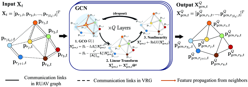
Figure 2: The structure of GCN.

The topology matrix $\mathbf{X}^{k^{*}}_{t}$ in (III-B1) only satisfies the constraint (10a), while does not minimize the objective function ${J}_{s}$. Therefore, to minimize ${J}_{s}$, we further extend the GCO $G(\cdot)$ to a graph convolutional network (GCN). As shown in Fig. 2, the GCN is composed of $Q$ graph convolutional layers (GCLs), where $Q\in\mathbb{N}_{+}$ is a hyperparameter. The $q$-th GCL receives a topology matrix $\mathbf{X}^{q-1}_{gcn,t}$ from the $(q-1)$-th GCL and outputs a topology matrix $\mathbf{X}^{q}_{gcn,t}$ to the next GCL, $q\in\{1,2,...,Q\}$. Specifically, in the $q$-th GCL, $\mathbf{X}^{q-1}_{gcn,t}$ is processed by the GCO $G(\cdot)$ as

$$\mathbf{X}^{q}_{gcn,t}=(\mathbf{I}_{t}-H_{t}\mathbf{L}^{v}_{t})\mathbf{X}^{q-1}_{gcn,t}=\big{(}\mathbf{I}_{t}-\frac{\epsilon^{*}}{\left\|\mathbf{A}^{v}_{t}\right\|_{\infty}}\mathbf{L}^{v}_{t}\big{)}\mathbf{X}^{q-1}_{gcn,t}.$$ (21)

Then the $\mathbf{X}^{q}_{gcn,t}$ is linearly transformed as

$$\mathbf{X}^{q}_{gcn,t}\leftarrow\mathbf{X}^{q}_{gcn,t}\mathbf{\Theta}^{q},$$ (22)

where $\mathbf{\Theta}^{q}$ is the trainable parameter of the $q$-th GCL. In addition, nonlinearities are introduced to the $q$-th GCL by applying the ReLU activation function to $\mathbf{X}^{q}_{gcn,t}$ as

$$\mathbf{X}^{q}_{gcn,t}\leftarrow\text{ReLU}(\mathbf{X}^{q}_{gcn,t}).$$ (23)

Hence, the relationship between $\mathbf{X}^{q}_{gcn,t}$ and $\mathbf{X}^{q-1}_{gcn,t}$ can be expressed as

$$\mathbf{X}^{q}_{gcn,t}=\underbrace{\text{ReLU}\bigg{(}}_{{\text{nonlinearity}}}\underbrace{\big{(}\mathbf{I}_{t}-\frac{\epsilon^{*}}{\left\|\mathbf{A}^{v}_{t}\right\|_{\infty}}\mathbf{L}^{v}_{t}\big{)}}_{{\text{GCO }G(\cdot)}}\underbrace{\mathbf{X}^{q-1}_{gcn,t}\mathbf{\Theta}^{q}\bigg{)}}_{{\text{linear transformation}}}.$$ (24)

Note that dropouts[38] can be added between two GCLs to increase the generalization ability of the GCN. The output topology matrix $\mathbf{X}^{Q}_{gcn,t}=[\mathbf{p}^{Q}_{gcn,r_{1},t},\mathbf{p}^{Q}_{gcn,r_{2},t},...,\mathbf{p}^{Q}_{gcn,r_{|\mathcal{I}_{t}|},t}]^{T}$ of the GCN can form a new RUAV graph $\mathcal{G}^{Q}_{t}=\{\mathcal{R}_{t},\mathcal{E}^{Q}_{gcn,t},\mathbf{X}^{Q}_{gcn,t}\}$, where the edge set ${\mathcal{E}}_{gcn,t}^{Q}=\{e_{ii^{\prime},t}|{l}_{ii^{\prime},t}=\left\|\mathbf{p}^{Q}_{gcn,i,t}-\mathbf{p}^{Q}_{gcn,i^{\prime},t}\right\|_{2}\text{satisfies CLEC},\forall i\neq i^{\prime},i,i^{\prime}\in\mathcal{I}_{t}\}$. Denote the number of RUAV clusters of the RUAV graph $\mathcal{G}^{Q}_{t}$ as $C^{Q}_{t}$.

III-B4 Loss function design of the GCN

Denote the loss function of the GCN as $\mathcal{L}(\mathbf{\Theta},\mathbf{X}_{t})$, where $\mathbf{\Theta}=\{\mathbf{\Theta}^{1},\mathbf{\Theta}^{2},...,\mathbf{\Theta}^{Q}\}$, and $\mathbf{X}_{t}$ is the input topology matrix to the GCN. The design of $\mathcal{L}(\mathbf{\Theta},\mathbf{X}_{t})$ should be consistent with $(\mathbf{P1})$. Specifically, we rewrite $(\mathbf{P1})$ as

$$(\mathbf{P1^{\dagger}}):\quad\;\min_{\mathbf{X}^{Q}_{gcn,t}}\quad {J}_{s}=\max_{i\in\mathcal{I}_{t}}\left\|\mathbf{p}^{Q}_{gcn,i,t}-\mathbf{p}_{i,t}\right\|_{2}$$ (25)

$$\operatorname{s.t.}\quad C^{Q}_{t}-1\leq 0,$$ (25a)

where $\widetilde{\mathbf{X}}_{t}$ in $(\mathbf{P1})$ is substituted by the output of the GCN $\mathbf{X}^{Q}_{gcn,t}$, and the constraint (10a) is represented by $C^{Q}_{t}-1\leq 0$. Then, we design $\mathcal{L}(\mathbf{\Theta},\mathbf{X}_{t})$ as the Lagrange function of $(\mathbf{P1^{\dagger}})$ as

$$\mathcal{L}(\mathbf{\Theta},\mathbf{X}_{t})=\underbrace{\tau(C^{Q}_{t}-1)}_{{\text{guarantee the CCN}}}+\underbrace{\max_{i\in\mathcal{I}_{t}}\left\|\mathbf{p}^{Q}_{gcn,i,t}-\mathbf{p}_{i,t}\right\|_{2}}_{{\text{minimize the largest displacement}}},$$ (26)

where the Lagrange multiplier $\tau$ is set as a positive constant. After training the GCN with the designed loss function $\mathcal{L}(\mathbf{\Theta},\mathbf{X}_{t})$, the output topology matrix $\mathbf{X}^{Q}_{gcn,t}$ of the GCN can approximate the solution to $(\mathbf{P1})$, i.e., $\mathbf{X}^{Q}_{gcn,t}\rightarrow\widetilde{\mathbf{X}}_{t}$.

III-B5 Off-line meta learning scheme

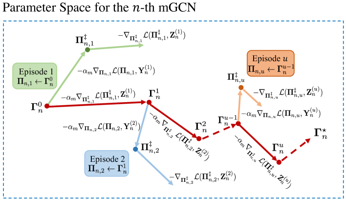
Figure 3: Meta learning procedure for the $n$-th mGCN.

Notice that different cases of UEDs will result in distinct topology matrices $\mathbf{X}_{t}$, leading to different loss functions $\mathcal{L}(\mathbf{\Theta},\mathbf{X}_{t})$ for the GCN. Hence, the GCN should be trained again in an on-line manner when encountering new cases of UEDs. However, training the GCN from scratch is time consuming and cannot be executed in real-time. Moreover, since there are infinite topology matrices, we cannot train the GCN in advance for each topology matrix. To address these issues, we propose a meta learning scheme for the GCN. The meta learning scheme can find promising initial parameters in an off-line manner to facilitate the on-line trainings [39]. Specifically, for a USNET with $N$ UAVs initially, the number $n$ of the RUAVs after one-off UEDs can only be in the range of $\{0,1,2,...,N\}$. We do not need to consider the cases when $n=0$ and $n=1$, since there is either no RUAVs or only one UAV that can form a CCN itself. For the other $N-1$ cases, we build $N-1$ GCNs with the same structures as Fig. 2, named meta GCNs (mGCNs). The $n$-th mGCN specifically deals with the case where the number of RUAVs is $n$, $n\in\{2,3,...,N\}$. For the $n$-th mGCN, we construct a support set $\mathcal{S}_{n}=\{\mathbf{Y}^{(1)}_{n},\mathbf{Y}^{(2)}_{n},...,\mathbf{Y}^{(U_{0})}_{n}\}$ with $U_{0}$ support data $\mathbf{Y}^{(u)}_{n}$, where $U_{0}\in\mathbb{N}_{+}$ is the size of $\mathcal{S}_{n}$, and $\mathbf{Y}^{(u)}_{n}=[\mathbf{p}^{(u,1)}_{n,spt},\mathbf{p}^{(u,2)}_{n,spt},...,\mathbf{p}^{(u,n)}_{n,spt}]^{T}$ is a randomly generated topology matrix with size $n\times 3$ under the constraint that $\mathbf{Y}^{(u)}_{n}$ cannot make the RUAV graph $\mathcal{G}_{t}$ form a CCN, $u\in\{1,2,...,U_{0}\}$. Meanwhile, we construct a query set $\mathcal{W}_{n}=\{\mathbf{Z}^{(1)}_{n},\mathbf{Z}^{(2)}_{n},...,\mathbf{Z}^{(U_{0})}_{n}\}$ with $U_{0}$ query data $\mathbf{Z}^{(u)}_{n}$, where $\mathbf{Z}^{(u)}_{n}=[\mathbf{p}^{(u,1)}_{n,qur},\mathbf{p}^{(u,2)}_{n,qur},...,\mathbf{p}^{(u,n)}_{n,qur}]^{T}$ is also a randomly generated topology matrix with size $n\times 3$ under the constraint that $\mathbf{Z}^{(u)}_{n}$ cannot make the RUAV graph $\mathcal{G}_{t}$ form a CCN. We carry out the meta learning in an off-line manner for the $n$-th mGCN, as shown in Fig. 3. The number of episodes of the meta learning equals to the size $U_{0}$ of $\mathcal{S}_{n}$ (or $\mathcal{W}_{n}$). In the $u$-th episode, we take $\mathbf{Y}^{(u)}_{n}$ in $\mathcal{S}_{n}$ and $\mathbf{Z}^{(u)}_{n}$ in $\mathcal{W}_{n}$ to update the parameter of the $n$-th mGCN at the $u$-th episode $\mathbf{\Gamma}^{u-1}_{n}$. Specifically, a temporary GCN in Fig. 2 with parameter ${\mathbf{\Pi}}_{n,u}$ is endowed with $\mathbf{\Gamma}^{u-1}_{n}$, i.e., ${\mathbf{\Pi}}_{n,u}\leftarrow\mathbf{\Gamma}^{u-1}_{n}$. The parameter ${\mathbf{\Pi}}_{n,u}$ is updated in the direction of $\nabla_{{\mathbf{\Pi}}_{n,u}}\mathcal{L}({\mathbf{\Pi}}_{n,u},\mathbf{Y}^{(u)}_{n})$ by $\alpha_{{meta}}>0$ step size, i.e.,

$${\mathbf{\Pi}}_{n,u}^{\ddagger} ={\mathbf{\Pi}}_{n,u}-\alpha_{{meta}}\nabla_{\mathbf{\Pi}_{n,u}}\mathcal{L}(\mathbf{\Pi}_{n,u},\mathbf{Y}^{(u)}_{n})$$

$$=\mathbf{\Gamma}^{u-1}_{n}-\alpha_{{meta}}\nabla_{\mathbf{\Pi}_{n,u}}\bigg{[}\tau(C^{u,temp}_{n,spt}-1)+$$

$$\qquad\quad\max_{n_{\beta}\in\{1,2,...,n\}}\left\|\mathbf{p}^{(u,n_{\beta},temp)}_{n,spt}-\mathbf{p}_{n,spt}^{(u,n_{\beta})}\right\|_{2}\bigg{]},$$ (27)

where $\mathbf{\Pi}_{n,u}^{\ddagger}$ is the updated parameter of the temporary GCN, $\mathbf{p}^{(u,n_{\beta},temp)}_{n,spt}$ is the $n_{\beta}$-th row in the output $\mathbf{X}^{(u,temp)}_{n,spt}$ of the temporary GCN, and $C^{u,temp}_{n,spt}$ is the number of RUAV clusters of the RUAV graph $\mathcal{G}_{t}$ formed by $\mathbf{X}^{(u,temp)}_{n,spt}$. The parameter of the $n$-th mGCN is updated in the direction of $\nabla_{\mathbf{\Pi}_{n,u}^{\prime}}\mathcal{L}(\mathbf{\Pi}_{n,u}^{\ddagger},\mathbf{Z}^{(u)}_{n})$ by $\alpha_{{meta}}$ step size, i.e.,

$$\mathbf{\Gamma}^{u}_{n} =\mathbf{\Gamma}^{u-1}_{n}-\alpha_{{meta}}\nabla_{\mathbf{\Pi}_{n,u}^{\ddagger}}\mathcal{L}(\mathbf{\Pi}_{n,u}^{\ddagger},\mathbf{Z}^{(u)}_{n})$$

$$=\mathbf{\Gamma}^{u-1}_{n}-\alpha_{{meta}}\nabla_{\mathbf{\Pi}_{n,u}^{\ddagger}}\bigg{[}\tau(C^{u,temp}_{n,qur}-1)+$$

$$\qquad\qquad\max_{n_{\beta}\in\{1,2,...,n\}}\left\|\mathbf{p}^{(u,n_{\beta},temp)}_{n,qur}-\mathbf{p}_{n,qur}^{(u,n_{\beta})}\right\|_{2}\bigg{]},$$ (28)

where $\mathbf{p}^{(u,j,temp)}_{n,qur}$ is the $u$-th row in the output $\mathbf{X}^{(u,temp)}_{n,qur}$ of the temporary GCN, and $C^{u,temp}_{n,qur}$ is the number of RUAV clusters of the RUAV graph $\mathcal{G}_{t}$ formed by $\mathbf{X}^{(u,temp)}_{n,qur}$. After $U_{0}$ episodes, we obtain the meta parameters of all the $N-1$ mGCNs $\mathbf{\Gamma}^{\star}_{n}\triangleq\mathbf{\Gamma}^{U_{0}}_{n}$ that act as the initial parameters for the GCNs during on-line executions.

III-B6 On-line executions of the GCN

When the USNET is destructed by one-off UEDs at time step $t$ and the RUAV graph $\mathcal{G}_{t}$ has $N_{0}\in\{2,3,...,N\}$ RUAVs, we build the VRG $\mathcal{G}_{t}^{v}=\{\mathcal{R}_{t}^{v},\mathcal{E}_{t}^{v},\mathbf{X}_{t}^{v}\}$, and calculate the Laplace matrix $\mathbf{L}^{v}_{t}$ for the GCN. Then the GCN will load the meta parameter $\mathbf{\Gamma}_{N_{0}}^{\star}$, i.e., $\mathbf{\Theta}\leftarrow\mathbf{\Gamma}_{N_{0}}^{\star}$. Next, the GCN will be trained on-line by the gradient descent of the loss function $\mathcal{L}(\mathbf{\Theta},\mathbf{X}_{t})$, i.e.,

$$\mathbf{\Theta}\leftarrow\mathbf{\Theta}-\alpha_{{meta}}\nabla_{\Theta}\mathcal{L}(\mathbf{\Theta},\mathbf{X}_{t}).$$ (29)

Note that the number of the on-line training episodes, denoted as $M$, is a constant positive integer. After the on-line training, we input $\mathbf{X}_{t}$ into the GCN, and the GCN outputs the topology matrix $\mathbf{X}^{Q}_{gcn,t}$ that acts as the solution to $(\mathbf{P1})$, i.e., $\widetilde{\mathbf{X}}_{t}\leftarrow\mathbf{X}^{Q}_{gcn,t}$. Each RUAV_i,t will fly at a constant speed ${\mathbf{v}}_{i,t}=\frac{v_{0}}{\left\|\mathbf{p}^{Q}_{gcn,i,t}-\mathbf{p}_{i,t}\right\|_{2}}(\mathbf{p}^{Q}_{gcn,i,t}-\mathbf{p}_{i,t})$ until reaching point $\mathbf{p}^{Q}_{gcn,i,t}$. The process of the CR-MGC algorithm is briefly summarized in Algorithm 2.

Algorithm 2 CR-MGC Algorithm (A Brief Process Summary)

Inputs: The initial RUAV graph $\mathcal{G}_{0}=\{\mathcal{R}_{0},\mathcal{E}_{0},\mathbf{X}_{0}\}$, and the initial index set of RUAVs $\mathcal{I}_{0}$.
Outputs: The solution $\widetilde{\mathbf{X}}_{t}$ to $(\mathbf{P1})$, the flying trajectories of all RUAVs.
Initializations: The parameters of mGCNs $\mathbf{\Gamma}_{n}^{0}$, the parameter of the GCN $\mathbf{\Theta}$, support sets $\mathcal{S}_{n}$ and query sets $\mathcal{W}_{n}$, $n\in\{2,3,...,N\}$. Conduct numerical experiments (shown in Section V-B) to determine the $\eta^{\star}$ and $\epsilon^{\star}$.
Off-line Meta Training:

1:for $n=2$ to $N$ do

2:     for $u=1$ to $U$ do

3:         Build the VRGs based on $\mathbf{Y}^{(u)}_{n}$ and $\mathbf{Z}^{(u)}_{n}$ separately, and derive the corresponding Laplace matrices. Train one step on parameter $\mathbf{\Gamma}_{n}^{u-1}$ using (III-B5), and update $\mathbf{\Gamma}_{n}^{u-1}$ using (III-B5).

4:     end for

5:end for

6:Obtain all the meta parameters $\mathbf{\Gamma}_{n}^{\star},n\in\{2,3,...,N\}$.

On-line Executions:

1:A random one-off UED happens at time step $t$, and the USNET is destructed into a RUAV graph $\mathcal{G}_{t}=\{\mathcal{R}_{t},\mathcal{E}_{t},\mathbf{X}_{t}\}$ with $n$ RUAVs.

2:Build the VRG $\mathcal{G}_{t}^{v}=\{\mathcal{R}_{t}^{v},\mathcal{E}_{t}^{v},\mathbf{X}_{t}^{v}\}$, and calculate the Laplace matrix $\mathbf{L}^{v}_{t}$ for the GCN.

3:The GCN loads the meta parameter $\mathbf{\Gamma}^{\star}_{n}$, i.e., $\mathbf{\Theta}\leftarrow\mathbf{\Gamma}^{\star}_{n}$.

4:Train $\mathbf{\Theta}$ with (29) $M$ episodes, and obtain the output $\mathbf{X}^{Q}_{gcn,t}$.

5:Let $\widetilde{\mathbf{X}}_{t}\leftarrow\mathbf{X}^{Q}_{gcn,t}$. Each RUAV_i,t flies at a constant speed ${\mathbf{v}}_{i,t}=\frac{v_{0}}{\left\|\mathbf{p}^{Q}_{gcn,i,t}-\mathbf{p}_{i,t}\right\|_{2}}(\mathbf{p}^{Q}_{gcn,i,t}-\mathbf{p}_{i,t})$, $\forall i\in\mathcal{I}_{t}$ until reach point $\mathbf{p}^{Q}_{gcn,i,t}$.

IV SCC Algorithm for General UEDs

In this section, let us consider the SCC problem under the general UEDs $(\mathbf{P2})$. To cope with the issue that RUAVs can only obtain partial information, we build an individual data base (IDB) model for each UAV and develop a monitoring mechanism that can detect UEDs and the position changing of UAVs. We then propose a self-healing trajectory planning algorithm based on monitoring mechanisms and CR-MGC to cope with the general UEDs.

IV-A Individual Database Model and Monitoring Mechanisms

We embed an IDB $\mathcal{D}_{i,t}=\{\widehat{\mathbf{p}}_{1,t}^{i},\widehat{\mathbf{p}}_{2,t}^{i},...,\widehat{\mathbf{p}}_{N,t}^{i}\}\cup\widehat{\mathcal{I}}^{i}_{t}$ inside the $i$-th UAV that contains two parts, namely the individual positions of all UAVs $\{\widehat{\mathbf{p}}_{1,t}^{i},\widehat{\mathbf{p}}_{2,t}^{i},...,\widehat{\mathbf{p}}_{N,t}^{i}\}$ and the individual index set of RUAVs (IISR) $\widehat{\mathcal{I}}^{i}_{t}$. The UAVs always know their own positions. Hence, the individual position $\widehat{\mathbf{p}}^{i}_{i,t}$ in $\mathcal{D}_{i,t}$ of RUAV_i,t equals to the position of RUAV_i,t at each time step $t$, i.e., $\widehat{\mathbf{p}}^{i}_{i,t}=\mathbf{p}_{i,t}$. During the self-healing process, the monitoring mechanism is realized through the updating of IDBs.

IV-A1 Monitoring the position changing of UAVs by updating the individual positions

At each time step $t$, RUAV_i,t broadcasts its own position $\mathbf{p}_{i,t}$ to other RUAVs in the same RUAV cluster through MCLs. To better exhibit the SCC algorithm, we ignore the time delay of data transmissions in MCLs, and assume the broadcasting can be completed at time step $t$. If RUAV_i,t receives $\mathbf{p}_{i^{\prime},t}$ at time step $t$, it updates the individual position of the $i^{\prime}$-th UAV in $D_{i,t}$; otherwise, the old individual position of the $i^{\prime}$-th UAV in $D_{i,t-1}$ of RUAV_i,t does not change, i.e.,

$$\widehat{\mathbf{p}}^{i}_{i^{\prime},t}\leftarrow\left\{\begin{aligned} \mathbf{p}_{i^{\prime},t},\quad\;&\mbox{if receives }\mathbf{p}_{i^{\prime},t};\\ \widehat{\mathbf{p}}^{i}_{i^{\prime},t-1},\;\;&\mbox{otherwise}.\end{aligned}\right.$$ (30)

IV-A2 Monitoring the UEDs by updating the IISR

When the $j$-th UAV is destructed at time step $t$, its neighbor RUAV_i,t will notice the destruction immediately and drop the index $j$ from $\widehat{\mathcal{I}}^{i}_{t}$, i.e.,

$$\widehat{\mathcal{I}}^{i}_{t}\leftarrow\widehat{\mathcal{I}}^{i}_{t-1}\backslash\{j\}.$$ (31)

RUAVs within the same RUAV cluster share their IISRs through broadcasting, and RUAV_i,t updates $\widehat{\mathcal{I}}^{i}_{t}$ by taking the intersections of all the received IISRs, i.e.,

$$\widehat{\mathcal{I}}^{i}_{t}\leftarrow\widehat{\mathcal{I}}^{i}_{t}\cap\widehat{\mathcal{I}}^{i_{1}}_{t}\cap\widehat{\mathcal{I}}^{i_{2}}_{t}\cap...\cap\widehat{\mathcal{I}}^{i_{h}}_{t}\cap...\cap\widehat{\mathcal{I}}^{i_{|\mathcal{C}_{i,t}|-1}}_{t},$$ (32)

where $\mathcal{C}_{i,t}$ represents the RUAV cluster containing RUAV_i,t, and $\widehat{\mathcal{I}}^{i_{h}}_{t}$ represents the received IISR, $i_{h}\in\mathcal{I}_{t},\;h\in\{1,2,...,|\mathcal{C}_{i,t}|-1\}$.

Algorithm 3 CR-MGCM for the $i$-th UAV based on its IDB

Input: The IDB $\mathcal{D}_{i,0}=\{\widehat{\mathbf{p}}_{1,0}^{i},\widehat{\mathbf{p}}_{2,0}^{i}\,...,\widehat{\mathbf{p}}_{N,0}^{i}\}\cup\widehat{\mathcal{I}}^{i}_{0}$, the $\eta^{\star}$, $\epsilon^{\star}$ and $\mathbf{\Gamma}^{\star}_{n},n\in\{2,3,...,N\}$.
Outputs: The speed ${\mathbf{v}}_{i,t}$ of the $i$-th UAV during $t\in\{1,2,...,T\}$.
Initializations: An inertia counter $C_{I}\leftarrow 0$, a target position $\mathbf{\Xi}_{i}\in\mathbb{R}^{3}$, and the inertia $\kappa>0$.

1:for $t=1$ to $T$ do

2:     Update IDBs to monitor the UEDs and position changing of UAVs with (30), (31), (32).

3:     Calculate the Laplace matrix $\mathbf{L}_{t}$ of the RUAV graph formed by $\{\widehat{\mathbf{p}}_{1,t}^{i},\widehat{\mathbf{p}}_{2,t}^{i}\,...,\widehat{\mathbf{p}}_{N,t}^{i}\}$.

4:     if $\Omega(\lambda=0|\mathbf{L}_{t})>1$ then

5:         if $C_{I}==0$ then

6:              Calculate the $d_{min,t}^{v}$ by Algorithm 1 with inputs $[\widehat{\mathbf{p}}_{r_{1},t}^{i},\widehat{\mathbf{p}}_{r_{2},t}^{i}\,...,\widehat{\mathbf{p}}_{r_{|\widehat{\mathcal{I}}_{t}^{i}|},t}^{i}]^{T}$ and $\widehat{\mathcal{I}}^{i}_{t}$, calculate the maximum threshold $d_{max,t}^{v}$ as $d_{max,t}^{v}=\max_{i^{\prime},i^{\prime\prime}\in\widehat{\mathcal{I}}_{t}^{i}}\{\left\|\widehat{\mathbf{p}}_{i^{\prime},t}^{i}-\widehat{\mathbf{p}}_{i^{\prime\prime},t}^{i}\right\|_{2}\}$, and then $d_{t}^{v}=\eta^{\star}d_{min,t}^{v}+(1-\eta^{\star})d_{max,t}^{v}$;

7:              Build the VRG $\mathcal{G}^{v}_{t}=\{\mathcal{R}_{t}^{v},\mathcal{E}^{v}_{t},\mathbf{X}^{v}_{t}\}$, where $\mathcal{R}_{t}^{v}=\{\text{RUAV}_{i,t}|i\in\widehat{\mathcal{I}}^{i}_{r,t}\}$, $\mathbf{X}^{v}_{t}=[\widehat{\mathbf{p}}_{r_{1},t}^{i},\widehat{\mathbf{p}}_{r_{2},t}^{i}\,...,\widehat{\mathbf{p}}_{r_{|\widehat{\mathcal{I}}_{t}^{i}|},t}^{i}]^{T}$, and $\mathcal{E}^{v}_{t}=\{e^{v}_{i^{\prime}i^{\prime\prime},t}|i^{\prime},i^{\prime\prime}\in\widehat{\mathcal{I}}_{t}^{i},i^{\prime}\neq i^{\prime\prime},\left\|\widehat{\mathbf{p}}^{i}_{i^{\prime},t}-\widehat{\mathbf{p}}^{i}_{i^{\prime\prime},t}\right\|_{2}\leq d_{t}^{v}\}$. Derive the Laplace matrix $\mathbf{L}^{v}_{t}$ of the VRG $\mathcal{G}^{v}_{t}$.

8:              Load $\mathbf{\Gamma}^{\star}_{|\widehat{\mathcal{I}}^{i}_{t}|}$ to the GCN, i.e., $\mathbf{\Theta}\leftarrow\mathbf{\Gamma}^{\star}_{|\widehat{\mathcal{I}}^{i}_{t}|}$, train the GCN $M$ episodes with (29).

9:              The GCN outputs $\mathbf{X}^{Q}_{gcn,t}=[\mathbf{p}^{Q}_{gcn,r_{1},t},\mathbf{p}^{Q}_{gcn,r_{2},t},...,\mathbf{p}^{Q}_{gcn,r_{|\widehat{\mathcal{I}}^{i}_{r,t}|},t}]^{T}$ with input $\mathbf{X}^{v}_{i,t}$.

10:              Let $\mathbf{\Xi}_{i}\leftarrow\mathbf{p}^{Q}_{gcn,i,t}$, and ${\mathbf{v}}_{i,t}\leftarrow\frac{v_{0}}{\left\|\mathbf{\Xi}_{i}-\widehat{\mathbf{p}}^{i}_{i,t}\right\|_{2}}(\mathbf{\Xi}_{i}-\widehat{\mathbf{p}}^{i}_{i,t})$. Let $C_{I}\leftarrow C_{I}+1$.

11:         else

12:              ${\mathbf{v}}_{i,t}\leftarrow\frac{v_{0}}{\left\|\mathbf{\Xi}_{i}-\widehat{\mathbf{p}}^{i}_{i,t}\right\|_{2}}(\mathbf{\Xi}_{i}-\widehat{\mathbf{p}}^{i}_{i,t})$.

13:         end if

14:         Let $C_{I}\leftarrow 0$ if $C_{I}==\kappa$.

15:     else

16:         ${\mathbf{v}}_{i,t}=\mathbf{0}$, and $C_{I}\leftarrow 0$

17:     end if

18:     if the $i$-th UAV is destructed then

19:         break

20:     end if

21:end for

Define the global information $\mathcal{D}_{G,t}$ at time step $t$ as the union of the positions of all UAVs and the index set of RUAVs, i.e., $\mathcal{D}_{G,t}=\{\mathbf{p}_{1,t},\mathbf{p}_{2,t},...,\mathbf{p}_{N,t}\}\cup\mathcal{I}_{t}$. Note that the monitoring mechanism tries to help RUAVs obtain the latest information about the USNET as mush as possible, but still cannot help all the RUAVs obtain the global information $\mathcal{G}_{t}$ at each time step $t$. This means that there may exist some certain some time step $t$ at which $\mathcal{D}_{i,t}\neq\mathcal{D}_{G,t}$ for some RUAV_i,t. Nonetheless, at the time steps when the RUAV graph $\mathcal{G}_{t}$ forms a CCN, all the RUAVs can obtain the global information $\mathcal{D}_{G,t}$. For example, the USNET forms a CCN at $t=0$, and then there is $\mathcal{D}_{i,0}=\mathcal{D}_{G,0}$.

IV-B Self-healing Trajectory Planning Algorithm

Based on the CR-MGC and the monitoring mechanisms, we propose a self-healing trajectory planning algorithm, named CR-MGCM, to cope with the the general UEDs. The details of CR-MGCM algorithm for each UAV are stated in Algorithm 3. In a nutshell, each UAV first loads $\eta^{\star}$, $\epsilon^{\star}$, the meta parameters $\mathbf{\Gamma}_{n}^{\star}$, and the GCN with randomly initialized $\mathbf{\Theta}$. Then during on-line executions, each RUAV monitors the UEDs and position changing of UAVs by updating its IDB. RUAV_i,t determines its flying directions by carrying out the on-line execution part of CR-MGC based on the data in $\mathcal{D}_{i,t}$. Note that for each UAV we set an inertia $\kappa\;(\kappa>0)$ that determines the number of time steps to maintain the flying directions before rerunning the on-line execution part of the CR-MGC. The outputs of CR-MGCM of all UAVs act as the solution to $(\mathbf{P2})$.

IV-C Theoretical Effectiveness of CR-MGCM

If UAVs always have the global information $\mathcal{D}_{G,t}$, then the CR-MGCM can skip the monitoring mechanism in step “2” and simply let $\{\widehat{\mathbf{p}}_{1,t}^{i},\widehat{\mathbf{p}}_{2,t}^{i}\,...,\widehat{\mathbf{p}}_{N,t}^{i}\}\leftarrow\{{\mathbf{p}}_{1,t},{\mathbf{p}}_{2,t}\,...,{\mathbf{p}}_{N,t}\}$ and $\widehat{\mathcal{I}}_{t}^{i}\leftarrow{\mathcal{I}}_{t}$ for each RUAV_i,t in each time step $t$. We refer the CR-MGCM algorithm where UAVs always have the global information $\mathcal{D}_{G,t}$ as CR-MGCM_glob. Note that CR-MGCM_glob is equivalent to the CR-MGC when coping with each single one-off UEDs. Due to the effectiveness of CR-MGC, CR-MGCM_glob is effective under one-off UEDs. On the other hand, since the general UEDs can be viewed as the combination of several one-off UEDs at different time steps, the CR-MGCM_glob is effective under the general UEDs.

However, since RUAVs cannot obtain $\mathcal{D}_{G,t}$, they may fly towards wrong directions during the self-healing process, which can make SCC algorithms ineffective. Nonetheless, we prove that CR-MGCM can reach the performance of CR-MGCM_glob under the general UEDs.

Proposition 2.

When applying the GCOs $G(\cdot)$ to the topology matrix $\mathbf{X}_{t}$, the positions of all RUAVs are moving towards their center $\frac{1}{|\mathcal{I}_{t}|}\sum_{i\in\mathcal{I}_{t}}\mathbf{p}_{i,t}$.

Proof.

See Appendix C. ∎

Since the GCN is mainly composed of GCOs $G(\cdot)$, it tends to make RUAVs gather towards the center of their positions. However, CR-MGCM makes each RUAV_i,t fly towards the incomplete center $\frac{1}{|\widehat{\mathcal{I}}_{t}^{i}|}\sum_{i^{\prime}\in\widehat{\mathcal{I}}_{t}^{i}}\widehat{\mathbf{p}}_{i^{\prime},t}^{i}$ that is calculated by the data in $\mathcal{D}_{i,t}$, while the CR-MGCM_glob makes each RUAV_i,t fly towards the complete center $\frac{1}{|\mathcal{I}_{t}|}\sum_{i^{\prime}\in\mathcal{I}_{t}}\mathbf{p}_{i^{\prime},t}$.

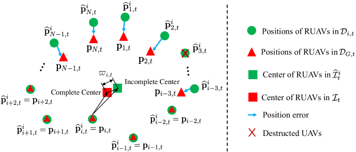
Figure 4: Individual positions in $\mathcal{D}_{i,t}$ and the RUAVs’ positions in global information $\mathcal{D}_{G,t}$.

TABLE II: Parameter settings of UAVs in the Simulations

Parameter	Values	Parameter description	Parameter	Values	Parameter description
$P$	30 dBm (=1W)	Transmitting signal power	$P_{0}$	1.38 dBm (=1.37mW)	Receiving signal power threshold
$G_{1}$,$G_{2}$	6 dBi	Antenna gain of receiving and transmitting signals	$\alpha$	1	$\alpha$ in (II-A)
$f_{c}$	2.4 GHz	Carrier frequency	$v_{c}$	$3\times 10^{8}$ m/s	Speed of light
$\sigma_{0}^{2}$	5	Strength of scattered path	$K$	10	Rice factor
$v_{0}$	1m/s	Magnitude of the speed of UAVs	$\alpha_{{meta}}$	0.01	learning rate in the meta learning

We then analyze the difference between the incomplete center and complete center for RUAV_i,t, as shown in Fig. 4. Denote the distance between two centers as $\varpi_{i,t}=\left\|\frac{1}{|\mathcal{I}_{t}|}\sum_{i^{\prime}\in\mathcal{I}_{t}}\mathbf{p}_{i^{\prime},t}-\frac{1}{|\widehat{\mathcal{I}}_{t}^{i}|}\sum_{i^{\prime}\in\widehat{\mathcal{I}}_{t}^{i}}\widehat{\mathbf{p}}_{i^{\prime},t}^{i}\right\|_{2}$, which can be expanded as (33). Notice that $\mathcal{I}_{t}\subseteq\widehat{\mathcal{I}}^{i}_{t}$ always holds for $\forall i\in\mathcal{I}_{t}$ and $\forall t\in\{1,2,...,T\}$, since $\widehat{\mathcal{I}}^{i}_{t}$ has no chance to drop the elements in $\mathcal{I}_{t}$. Hence, there is $\mathcal{I}_{t}\backslash\widehat{\mathcal{I}}^{i}_{t}=\varnothing$, which indicates $\sum_{i^{\prime}\in\mathcal{I}_{t}\backslash\widehat{\mathcal{I}}^{i}_{t}}\mathbf{p}_{i^{\prime},t}=\sum_{i^{\prime}\in\varnothing}\mathbf{p}_{i^{\prime},t}=0$. As the RUAVs initially store the global information $\mathcal{D}_{G,0}$, the incomplete center and complete center coincide at $t=0$, i.e., $\frac{1}{|\mathcal{I}_{0}|}\sum_{i^{\prime}\in\mathcal{I}_{0}}\mathbf{p}_{i^{\prime},0}=\frac{1}{|\widehat{\mathcal{I}}_{0}^{i}|}\sum_{i^{\prime}\in\widehat{\mathcal{I}}^{i}_{0}}\widehat{\mathbf{p}}_{i^{\prime},0}^{i}$. Moreover, the distance between $\widehat{\mathbf{p}}^{i}_{i^{\prime},t}$ and $\mathbf{p}_{i^{\prime},t}$ is bounded, since $\left\|\widehat{\mathbf{p}}^{i}_{i^{\prime},t}-\mathbf{p}_{i^{\prime},t}\right\|_{2}\leq vt<vT$ always holds. Therefore, we can assume the following three mild conditions:

• Position bound: $\left\|\widehat{\mathbf{p}}^{i}_{i^{\prime},t}-\mathbf{p}_{i^{\prime},t}\right\|_{2}\leq b_{1}<vT$, $b_{1}>0$ is a constant;

• Approximation of RUAV numbers: $\frac{1}{|\mathcal{I}_{t}|}\approx\frac{1}{|\widehat{\mathcal{I}}_{t}^{i}|}$;

• False RUAVs’ bound: $\left\|\frac{1}{|\widehat{\mathcal{I}}_{t}^{i}|}\sum_{i^{\prime}\in\mathcal{I}^{i}_{r,t}\backslash\mathcal{I}_{t}}\widehat{\mathbf{p}}^{i}_{i^{\prime},t}\right\|_{2}\leq b_{2}$, $b_{2}>0$ is a constant.

Then the upper bound of the distance $\varpi_{i,t}$ between incomplete center and complete center can be calculated as (IV-C), where $\mathcal{C}_{i,t}$ denotes the index set of RUAVs that are in the same RUAV cluster with RUAV_i,t. Hence, RUAVs using CR-MGCM nearly fly towards the same position as RUAVs using CR-MGCM_glob at each time step. Besides, the inertia $\kappa$ in CR-MGCM can offer RUAVs the latest information of USNET to plan their trajectories. Therefore, CR-MGCM can reach the performance of CR-MGCM_glob under the general UEDs.

 

$$\varpi_{i,t} =\left\|\sum_{i^{\prime}\in\mathcal{I}_{t}\cap\widehat{\mathcal{I}}^{i}_{t}}\bigg{(}\frac{1}{|\mathcal{I}_{t}|}\mathbf{p}_{i^{\prime},t}-\frac{1}{|\widehat{\mathcal{I}}_{t}^{i}|}\widehat{\mathbf{p}}_{i^{\prime},t}^{i}\bigg{)}+\frac{1}{|\mathcal{I}_{t}|}\sum_{i^{\prime}\in\mathcal{I}_{t}\backslash\mathcal{I}^{i}_{r,t}}\mathbf{p}_{i^{\prime},t}-\frac{1}{|\widehat{\mathcal{I}}_{t}^{i}|}\sum_{i^{\prime}\in\widehat{\mathcal{I}}^{i}_{t}\backslash\mathcal{I}_{t}}\widehat{\mathbf{p}}^{i}_{i^{\prime},t}\right\|_{2}.$$ (33)

 

$$\varpi_{i,t} =\left\|\frac{1}{|\mathcal{I}_{t}|}\sum_{i^{\prime}\in\mathcal{I}_{t}}\mathbf{p}_{i^{\prime},t}-\frac{1}{|\widehat{\mathcal{I}}_{t}^{i}|}\sum_{i^{\prime}\in\widehat{\mathcal{I}}_{t}^{i}}\mathbf{p}_{i^{\prime},t}^{i}\right\|_{2}=\left\|\sum_{i^{\prime}\in\mathcal{I}_{t}\cap\widehat{\mathcal{I}}_{t}^{i}}\bigg{(}\frac{1}{|\mathcal{I}_{t}|}\mathbf{p}_{i^{\prime},t}-\frac{1}{|\widehat{\mathcal{I}}_{t}^{i}|}\widehat{\mathbf{p}}_{i^{\prime},t}^{i}\bigg{)}-\frac{1}{|\widehat{\mathcal{I}}_{t}^{i}|}\sum_{i^{\prime}\in\widehat{\mathcal{I}}_{t}^{i}\backslash\mathcal{I}_{t}}\widehat{\mathbf{p}}^{i}_{i^{\prime},t}\right\|_{2}$$

$$\leq\left\|\sum_{i^{\prime}\in\mathcal{I}_{t}\cap\widehat{\mathcal{I}}_{t}^{i}\backslash\mathcal{C}_{i,t}}\frac{1}{|\mathcal{I}_{t}|}(\mathbf{p}_{i^{\prime},t}-\widehat{\mathbf{p}}_{i^{\prime},t}^{i})\right\|_{2}+\left\|\frac{1}{|\widehat{\mathcal{I}}_{t}^{i}|}\sum_{i^{\prime}\in\widehat{\mathcal{I}}_{t}^{i}\backslash\mathcal{I}_{t}}\widehat{\mathbf{p}}^{i}_{i^{\prime},t}\right\|_{2}\leq b_{1}+b_{2}.$$ (34)

 

V Simulation Results

In the simulation, the initial USNET consists of $N=200$ identical UAVs that are randomly distributed in a 1,000m$\times$1,000m$\times$100m three-dimensional space, as shown in Fig. 6. The parameters of UAVs are specified in Table II, and the CLEC can be calculated as

$$10\log_{10}\bigg{(}\frac{96\pi l_{ii^{\prime},t}}{3}\bigg{)}+\frac{l_{ii^{\prime},t}}{5}\exp\bigg{(}\frac{-l_{ii^{\prime},t}^{2}-100}{10}\bigg{)}I_{0}(20l_{ii^{\prime},t})$$

$$\approx 10\log_{10}\bigg{(}96l_{ii^{\prime},t}\bigg{)}\leq 40.62,$$ (35)

from which we can derive $l_{ii^{\prime},t}\approx 120\text{m}$. Hence, the CLEC can be described as: any two distinct UAVs can establish a communication link if their distance is smaller than 120m. The period of the self-healing process is set to be 450 time steps, i.e., $T=450$. The number of GCLs in the GCN is $Q=8$.

Figure 5: Initial distributions of the 200 identical UAVs .

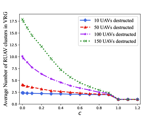
Figure 6: The average number of RUAV clusters versus $c$.

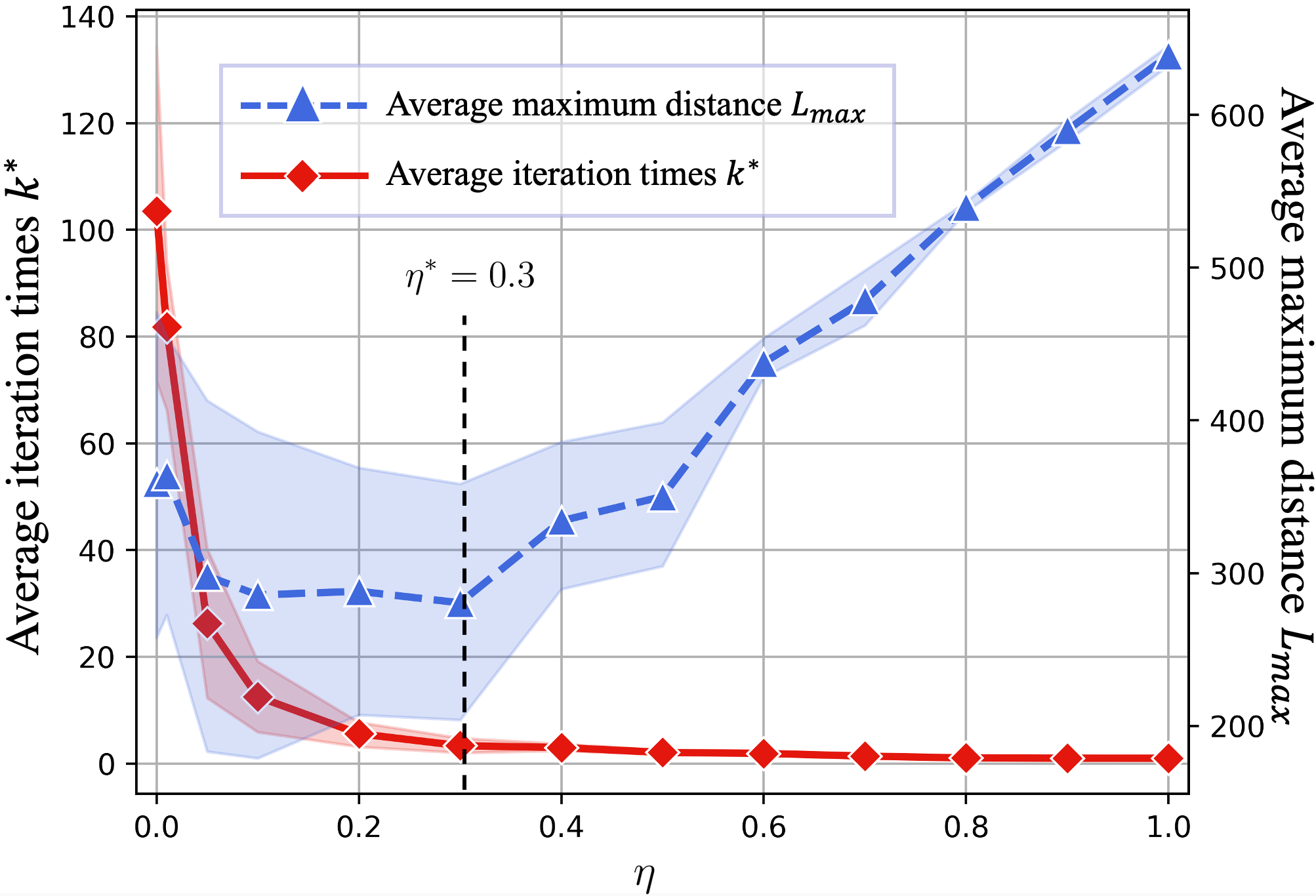
Figure 7: The average of $k^{*}$ versus $\eta$ and the average of $L_{max}$ versus $\eta$. The $\epsilon$ is $1$.

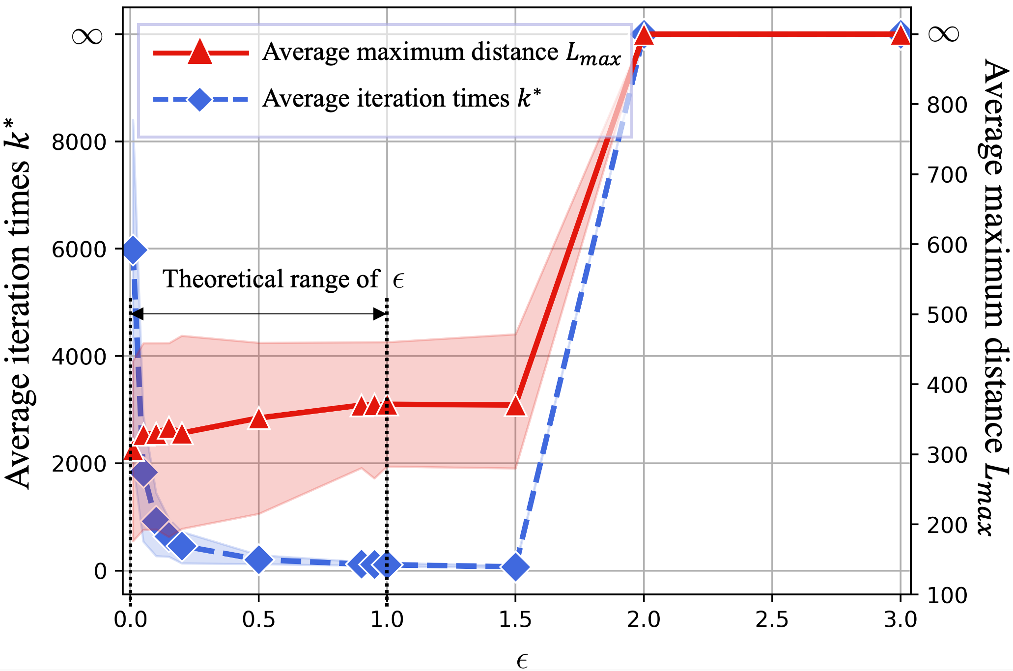
Figure 8: The average of $k^{*}$ versus $\epsilon$, and the average of $L_{max}$ versus $\epsilon$. The $\eta$ is $0.3$.

V-A Verifications of Algorithm 1

Express the virtual distance $d_{t}^{v}$ in the VRG as $d_{t}^{v}=120+c(d_{min,t}^{v}-120)$, where $d_{min,t}^{v}$ is obtained by Algorithm 1 and $c\geq 0$ is a coefficient. We randomly destroy 10, 50, 100 and 150 UAVs of the initial USNET 100 times each, and the average number of RUAV clusters in the VRG versus $c$ is shown in Fig. 6. When $c=0$ and $d_{t}^{v}=120$m, the average number of RUAV clusters is bigger than 1 and the VRG cannot form CCNs. As $c$ gets closer to 1, the virtual distance $d_{t}^{v}$ becomes larger and the average number of RUAV clusters in the VRG decreases. The VRG cannot form a CCN until $c=1$ and $d_{t}^{v}=d^{v}_{min,t}$. Hence, Algorithm 1 can guarantee to find the minimal virtual distance $d_{min,t}^{v}$ that makes the VRG a CCN.

V-B Finding $\eta^{\star}$ and $\epsilon^{\star}$ of the CR-MGC

We randomly destruct 10, 50, 100, 150 UAVs of the initial USNET 100 times each. Fig. 8 shows the average of the number of GCO $G(\cdot)$ iterations $k^{*}$ versus $\eta$. The average of $L_{max}$ versus $\eta$ is also shown in Fig. 7. We can see that the average of $k^{*}$ drops with the increase of $\eta$, while the average of $L_{max}$ slightly decreases when $\eta\leq 0.3$ and continuously increases when $\eta>0.3$. Hence, we choose $\eta^{\star}=0.3$ as the best value of $\eta$ to balance both $k^{*}$ and $L_{max}$.

We randomly destruct 10, 50, 100, 150 UAVs of the initial USNET 100 times each. Fig. 8 shows the average of $k^{*}$ versus $\epsilon$. The average of $L_{max}$ versus $\epsilon$ is also shown in Fig. 8 . When $\epsilon\in[0,1.5]$, the average of $k^{*}$ drops with the increase of $\epsilon$, while the average of $L_{max}$ increases. However, when $\epsilon>1.5$, the GCO diverges and both the average of $k^{*}$ and average of $L_{max}$ go to infinity. Recall that $H_{t}=\frac{\epsilon}{\left\|\mathbf{A}^{v}_{t}\right\|_{\infty}}$ and the theoretical range of $K_{t}$ is $0<H_{t}\leq\frac{1}{\left\|\mathbf{A}^{v}_{t}\right\|_{\infty}}$ (or equivalently $0<\epsilon\leq 1$). Hence, the results in Fig. 8 verify the correctness of the theoretical range of $H_{t}$. We can choose $\epsilon^{\star}=1$ as the best value of $\epsilon$ to balance both $k^{*}$ and $L_{max}$.

V-C Meta Learning of the GCN

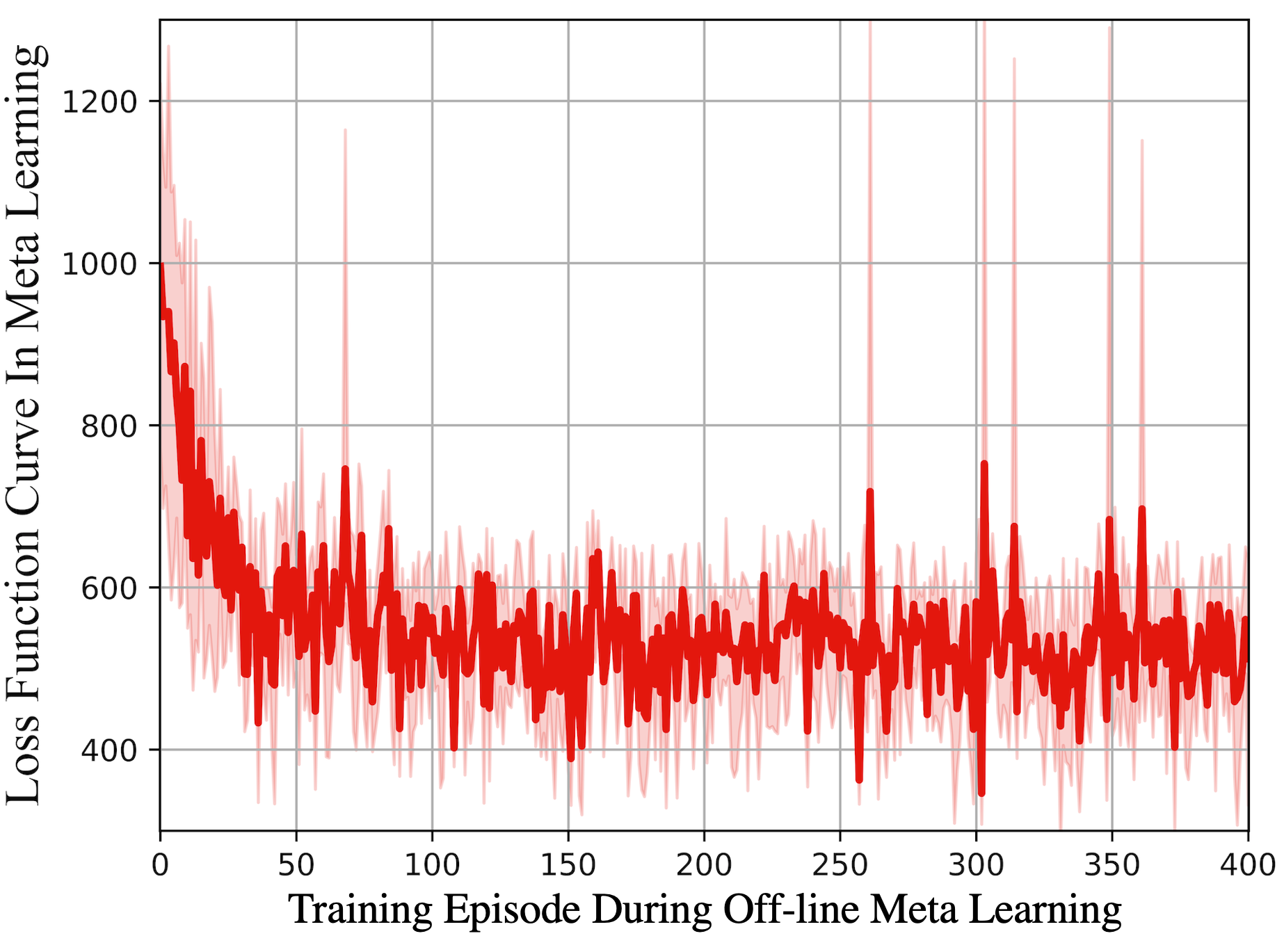
Figure 9: Loss function curve of the mGCNs during meta learning.

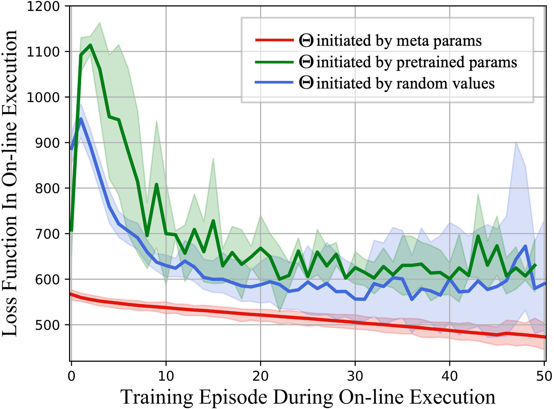
Figure 10: Loss function during the on-line executions, $M=50$.

We build $199$ mGCNs since the initial USNET contains $200$ UAVs. For each mGCN, we construct a support set and query set with $U_{0}=400$ topology matrices each. Fig. 10 shows the average loss function curve of all mGCNs during the off-line meta learning. We can see that the loss function starts from 1000 and drops stably to 500 during the off-line meta learning. The consistent decrease of the loss function indicates that the parameters of the mGCNs are gradually moving to better values.

Fig. 10 shows the loss function curves of the GCN during the training process in on-line executions, where the parameters of GCN $\mathbf{\Theta}$ are initiated by the meta parameters $\mathbf{\Gamma}^{\star}_{k}$, the pre-trained parameters, and random values, respectively. We set the on-line training episode to be $M=50$. On the one hand, the loss function curve of GCN initiated by meta parameters starts from 570 that is smaller than other two curves (700 and 900, respectively). This means that the meta parameters are better initialized values than both the pre-trained parameters and random parameters. On the other hand, the loss function curve of GCN initiated by meta parameters decreases continuously during the on-line training process and reaches lower values than other two curves, which implies the meta parameters have great potential in performance.

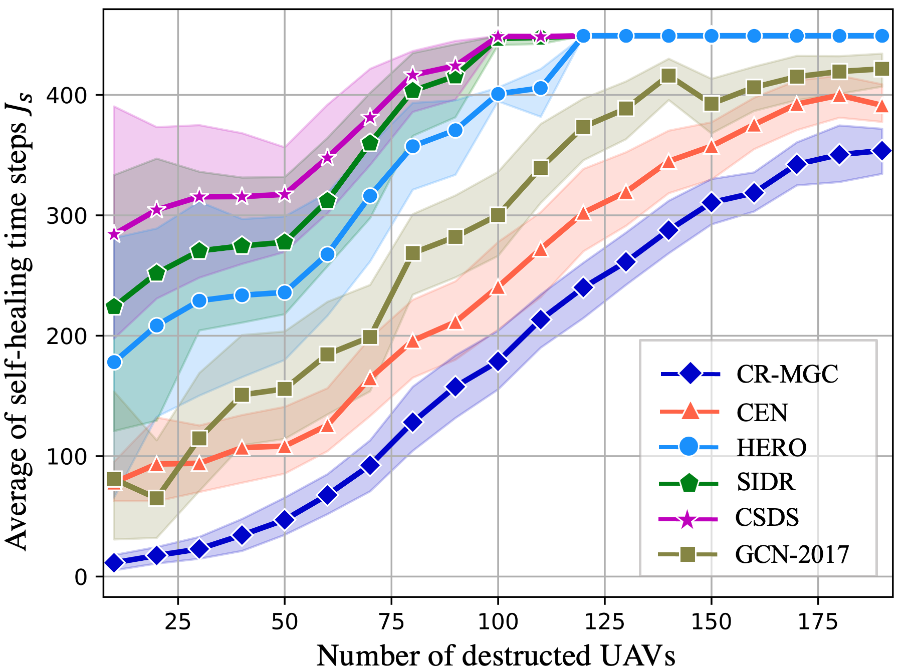
Figure 11: Average self-healing time steps ${J}_{s}$ under different number of destructed UAVs.

V-D SCC of One-off UEDs in $(\mathbf{P1})$

Fig. 11 shows the average self-healing time steps ${J}_{s}$ of the CR-MGC under one-off UEDs. The performances of HERO[20], SIDR[23], CSDS[19], GCN-2017[27], and CEN are also displayed for comparisons. We randomly destruct 10, 20, 30, …, 190 UAVs of the initial USNET 100 times each, and take the average value of the self-healing time to plot the curves of different algorithms. The shaded areas represent the 100% confidential intervals of the average self-healing time. We can see that with the increase of the number of destructed UAVs, the self-healing time of all the algorithms increases. Moreover, the average self-healing time of the CR-MGC is smaller than those of other four algorithms under any number of destructed UAVs. Hence, the CR-MGC can rebuild the communication connectivity of the USNET within shorter time.

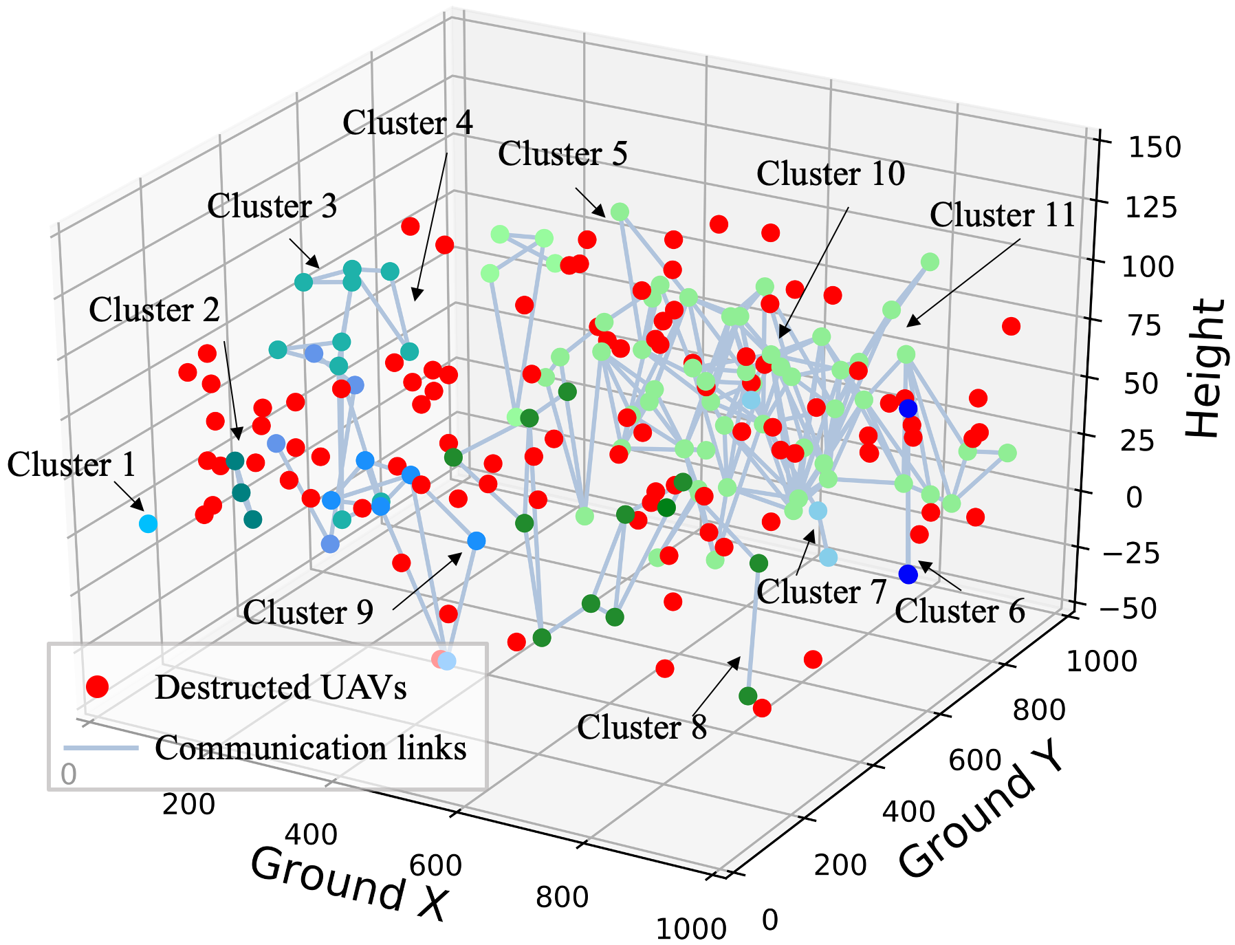
(a) The initial USNET is destructed into 11 RUAV clusters.

(b) The changing of the positions when applying the GCO $G(\cdot)$.

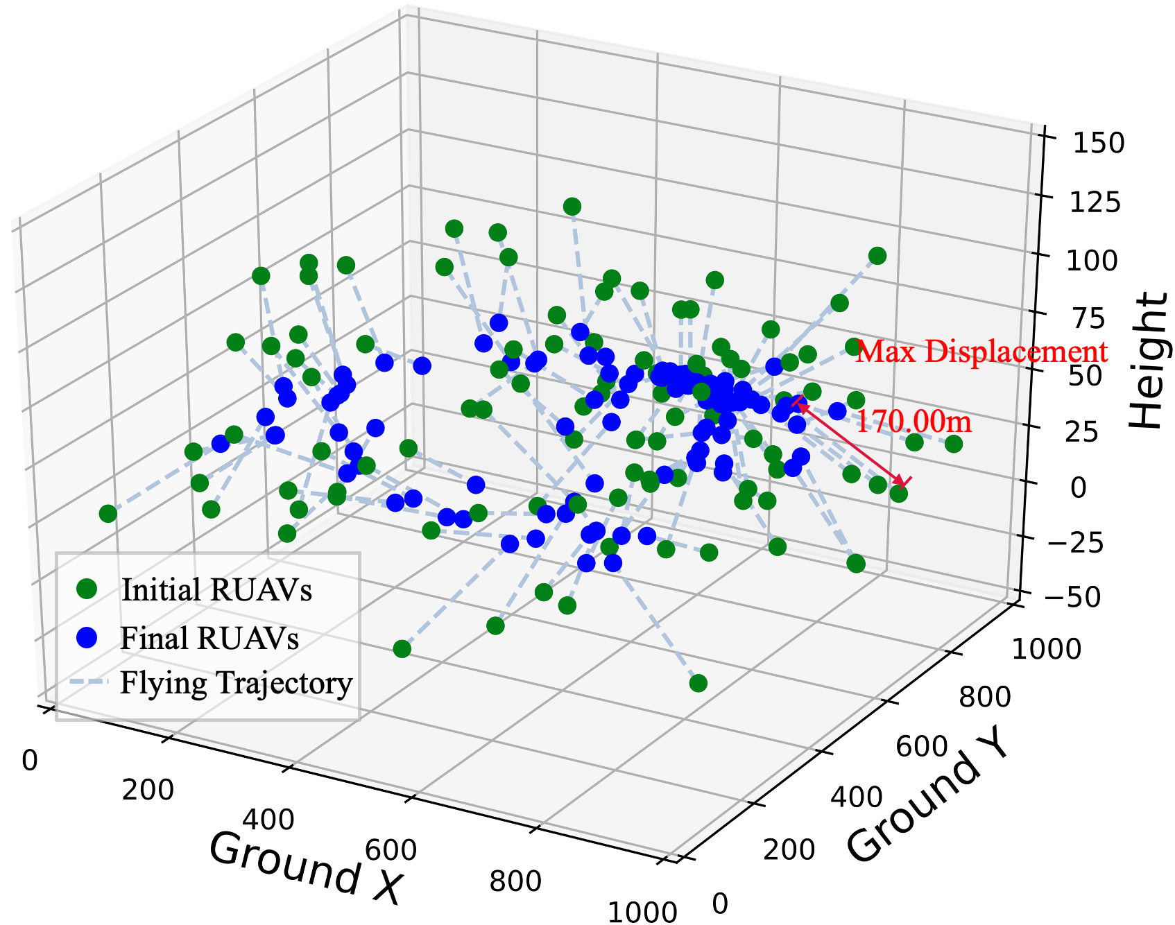
(c) Flying trajectories of RUAVs using CR-MGC.

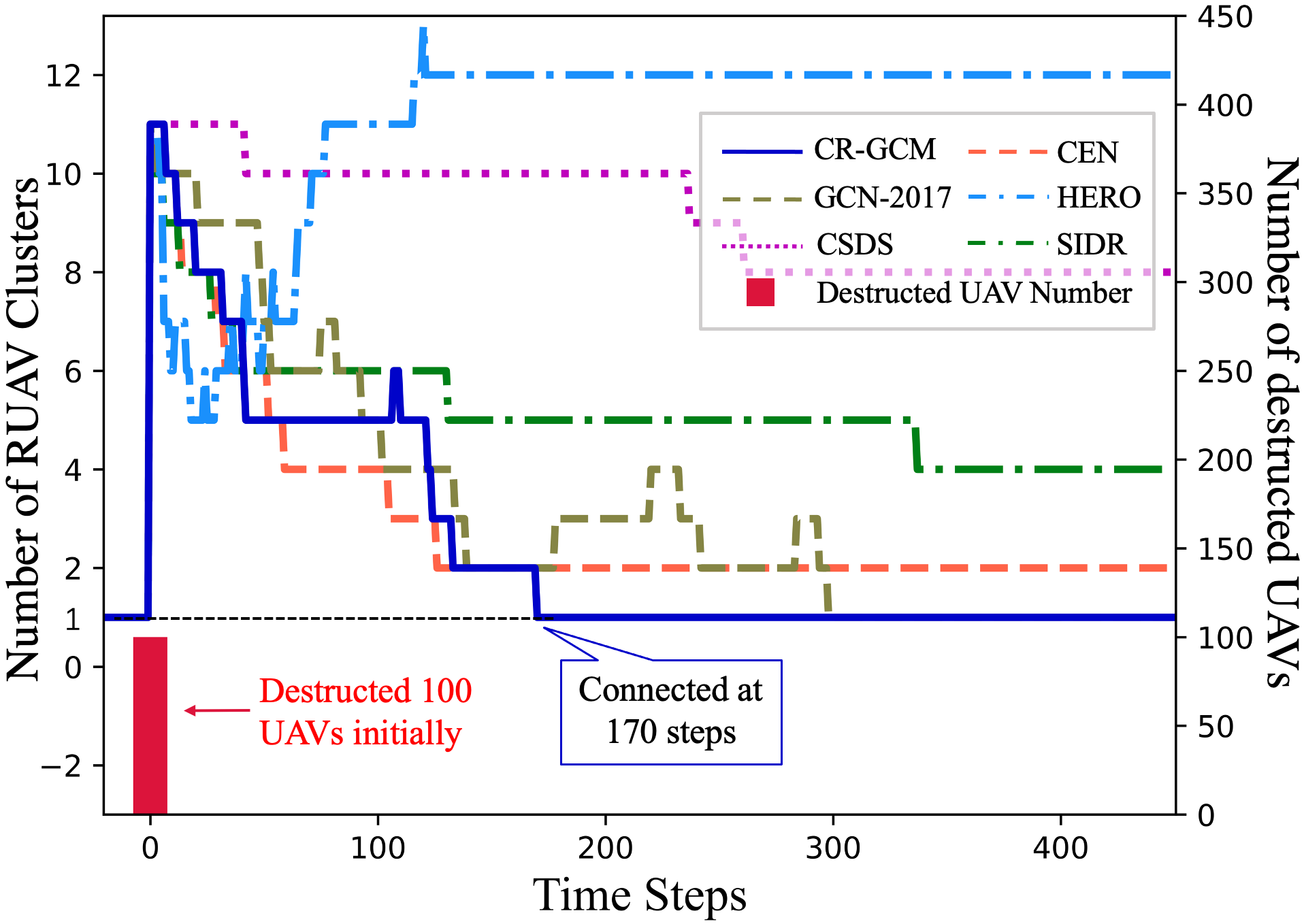
(d) The number of RUAV clusters versus the time steps.

Figure 12: Disruptions to the initial USNET and the self-healing process under different algorithms.

Fig. 12 shows the trajectories of the RUAVs during a certain self-healing process, where the one-off UED destroys $100$ UAVs at $t=0$. As shown in Fig. 12(a), the initial USNET is destructed into $C_{0}=11$ RUAV clusters, where nodes with the same color denotes the RUAVs in the same RUAV cluster. Fig. 12(b) shows that the GCOs can make the RUAVs gather towards their center to form a CCN, which is consistent with Proposition 2. Fig. 12(c) shows the flying trajectory of each RUAV using CR-MGC. The maximum displacement of all RUAVs is 170m. Fig. 12(d) shows that the number of RUAV clusters of the RUAV graph $\mathcal{G}_{t}$ decreases with CR-MGC. Moreover, the CR-MGC makes the RUAVs form a CCN within the least time steps.

V-E SCC of General UEDs in $(\mathbf{P2})$

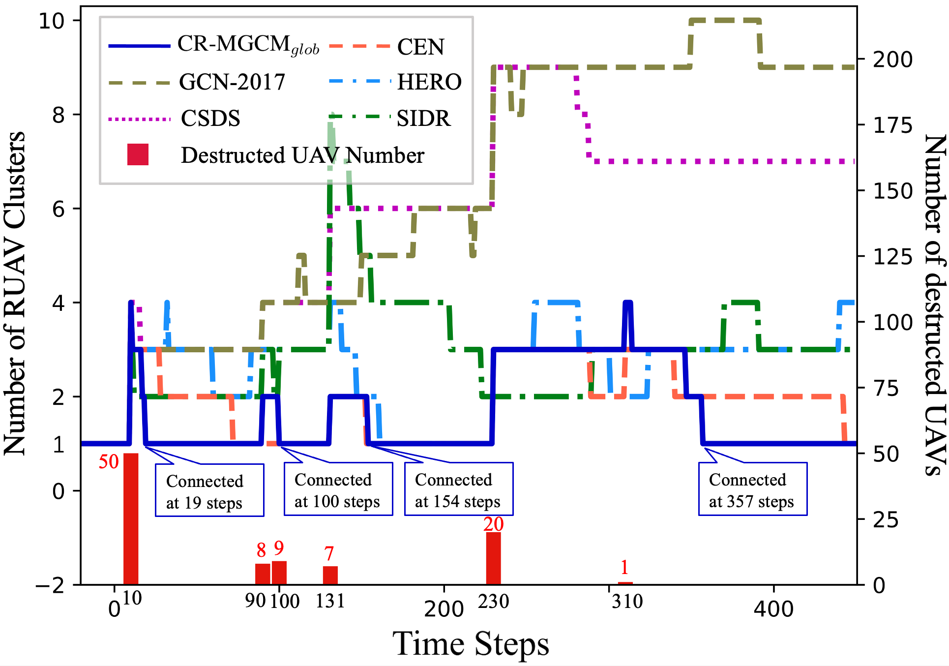
Figure 13: The number of RUAV cluster versus time steps under the general UEDs with global information.

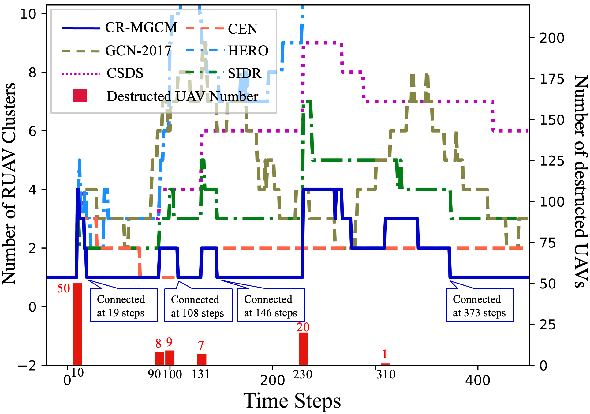
Figure 14: The number of RUAV cluster versus time steps under the general UEDs with monitoring mechanisms.

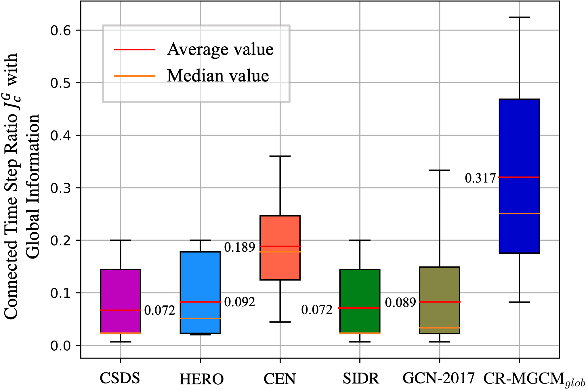
Figure 15: The connected time step ratio ${J}_{c}^{G}$ of different algorithms with global information.

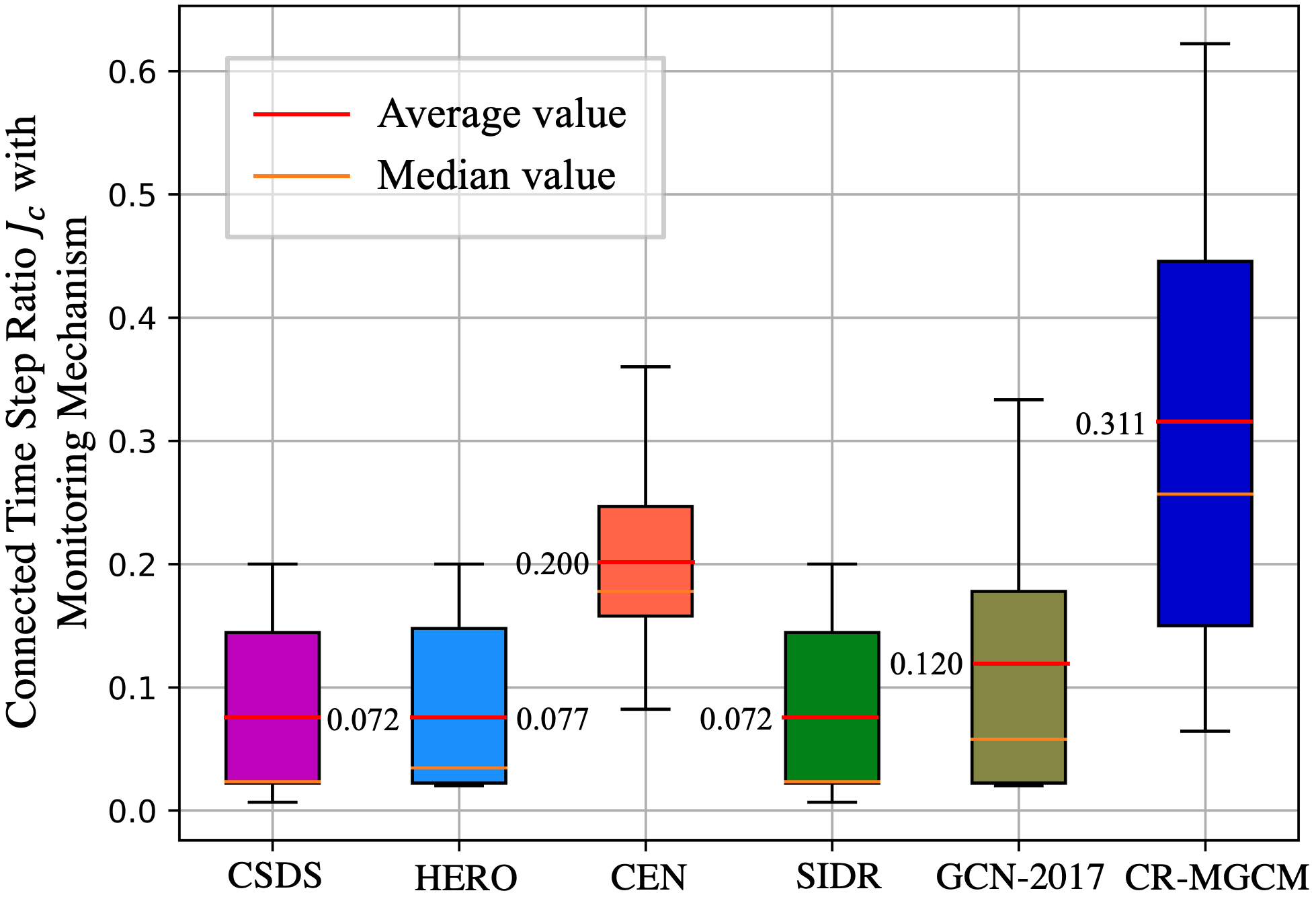
Figure 16: The connected time step ratio ${J}_{c}$ of different algorithms with monitoring mechanisms.

Fig. 14 and Fig. 14 both show the number of RUAV clusters $C_{t}$ using different algorithms under the same general UED. However, the RUAVs in the simulation of Fig. 14 have global information at each time step, while the RUAVs in the simulation of Fig. 14 do not and can only utilize the monitoring mechanism. The UED happens at 10, 90, 100, 131, and 230 time step and destruct 50, 8, 9, 7, and 20 UAVs, respectively. We can see that the RUAVs using CR-MGCM_glob and CR-MGCM both quickly forms a CCN after each UED, while the RUAVs using other algorithms slowly forms a CCN after UEDs or even cannot form CCNs. Hence, CR-MGCM_glob and CR-MGCM can effectively rebuild the communication connectivity of the USNET within shorter time steps than the existing algorithms.

We destructed the USNET with 10 distinct general UEDs and depict the distribution of the connected time step ratio by boxplots shown in Fig. 16 and Fig. 16. The RUAVs in the simulation of Fig. 16 have global information at each time step, while the RUAVs in the simulation of Fig. 16 only utilize the monitoring mechanism. In order to distinguish from $J_{c}$, we denote the connected time step ratio in Fig. 16 as $J_{c}^{G}$. We can see that the average ${J}_{c}^{G}$ with CR-MGCM_glob is larger than that of other algorithms, which indicates the effectiveness of the CR-MGCM_glob under the general UEDs. We can also see that the average ${J}_{c}$ with CR-MGCM is larger than that of other algorithms, which indicates the effectiveness of the CR-MGCM under the general UEDs. Moreover, the ratio between the average $J_{c}$ with CR-MGCM and the average $J_{c}^{G}$ with CR-MGCM_glob is $\frac{{J}_{c}}{{J}_{c}^{G}}=\frac{0.311}{0.317}=98.11\%$, which indicates that CR-MGCM can reach the performance of CR-MGCM_glob under the general UEDs.

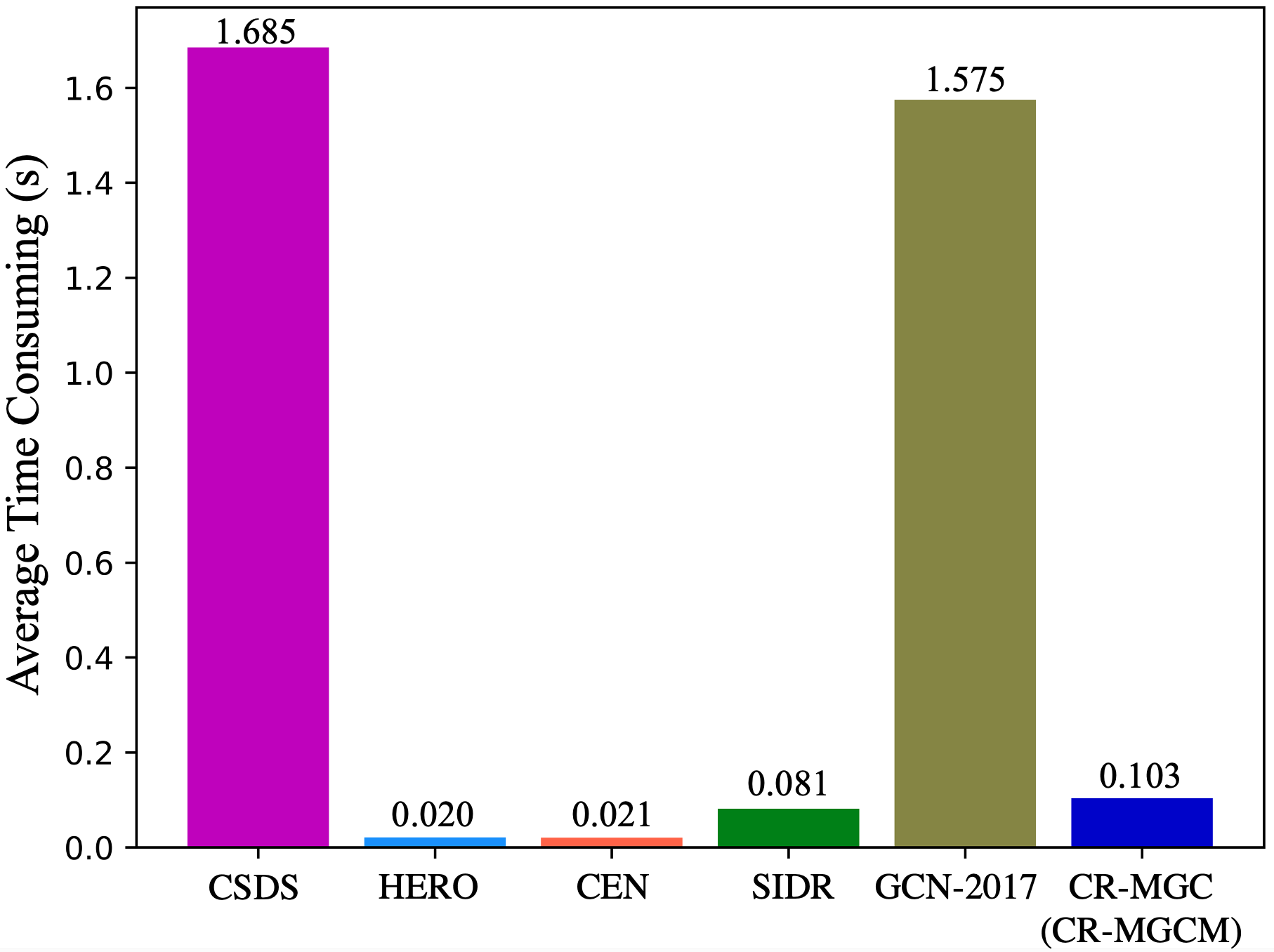
Figure 17: Average time consumptions of on-line executions with different algorithms.

V-F Time Consuming Comparisons

Fig. 17 compares the average on-line execution time cost at one time step of different algorithms. We can see that the average time cost of CR-MGC have the same magnitudes with HERO, CEN and SIDR, but is much smaller than CSDS and GCN-2017. Note that the CR-MGCM and CR-MGCM_glob both have the same time costs with CR-MGC, since they use the same GCN structures. This indicates that CR-MGC, CR-MGCM and CR-MGCM_glob have acceptable on-line execution time costs.

VI Conclusion

In this paper, we studied the SCC problem of the USNET under one-off UEDs and general UEDs. Specifically, we proposed a CR-MGC algorithm to cope with the SCC problem under one-off UEDs and verify its convergence. We also developed a meta learning scheme to improve the on-line executions of CR-MGC. For the SCC problem under the general UEDs, we designed the CR-MGCM algorithm to plan the trajectories of RUAVs. Numerical results showed that the proposed algorithms can rebuild the communication connectivity of the USNET within shorter time than the existing algorithms under both one-off UEDs and general UEDs. The experiment results also showed that the meta learning scheme could not only enhance the performance of the proposed algorithms, but also reduce the on-line execution time costs of them.

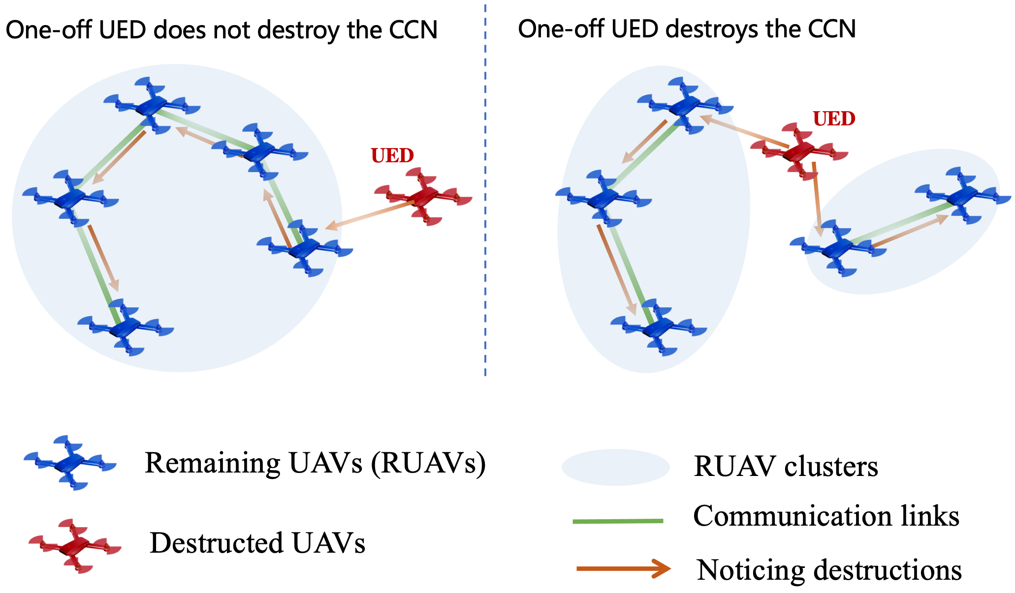
Figure 18: Examples of one-off UEDs to the same USNET. The left one-off UED does not destroy the CCN, while the right one-off UED destroys the CCN.

Appendix A Illustrations of One-off UEDs cases

Consider a USNET composed of $N$ UAVs with fixed initial positions $\{\mathbf{p}_{1,0},\mathbf{p}_{2,0},...,\mathbf{p}_{N,0}\}$. The one-off UED can destruct any number of UAVs with random indexes in the USNET at a certain time step. Denote the number of destructed UAVs as $\Upsilon\in\{1,2,...,N\}$. The number of cases of destructing $\Upsilon$ UAVs can be calculated as $C^{\Upsilon}_{N}=\frac{N!}{\Upsilon!(N-\Upsilon)!}$, where $C$ is the combinatorial number. Hence, the total number of one-off UED cases is $\sum_{\Upsilon=1}^{N}C_{N}^{\Upsilon}=2^{N}$.

Note that not all cases of one-off UEDs can destroy the communication connectivity of the USNET. For example, as shown in Fig. 18, the one-off UED on the left does not destroy the CCN, while the one-off UED on the right destroys the CCN. The RUAVs can stay still if they remain a CCN after the one-off UED. Therefore, we only consider the one-off UEDs that can destroy the communication connectivity of the USNET.

Appendix B Proof of Proposition 1

We first prove that the metric space $\{\mathbf{X}_{t}\mid\frac{1}{|\mathcal{I}_{t}|}\sum_{i\in\mathcal{I}_{t}}\mathbf{p}_{i,t}=\mathbf{c}\}$ is closed under the GCO $G(\cdot)$, i.e.,

$$G(\cdot):\{\mathbf{X}_{t}\mid\frac{1}{|\mathcal{I}_{t}|}\sum_{i\in\mathcal{I}_{t}}\mathbf{p}_{i,t}=\mathbf{c}\}\rightarrow\{\mathbf{X}_{t}\mid\frac{1}{|\mathcal{I}_{t}|}\sum_{i\in\mathcal{I}_{t}}\mathbf{p}_{i,t}=\mathbf{c}\}.$$ (36)

Then we prove that the GCO $G(\cdot)$ satisfies the contraction mapping theorem [37] when $0<H_{t}\leq\frac{1}{\left\|\mathbf{A}^{v}_{t}\right\|_{\infty}}$. In addition, we prove that the positions of RUAVs in the topology matrix $\overline{\mathbf{X}}_{t}$ (Banach point [37]) of the GCO $G(\cdot)$ all have the same value $\mathbf{c}$, i.e., $\overline{\mathbf{X}}_{t}=[\mathbf{c},\mathbf{c},...,\mathbf{c}]^{T}$.

B-A The Closure of GCO $G(\cdot)$ in $\{\mathbf{X}_{t}\mid\frac{1}{|\mathcal{I}_{t}|}\sum_{i\in\mathcal{I}_{t}}\mathbf{p}_{i,t}=\mathbf{c}\}$

We need to prove that $\forall\mathbf{X}_{t}\in\{\mathbf{X}_{t}\mid\frac{1}{|\mathcal{I}_{t}|}\sum_{i\in\mathcal{I}_{t}}\mathbf{p}_{i,t}=\mathbf{c}\}$, $\mathbf{X}^{1}_{t}=G(\mathbf{X}_{t})\in\{\mathbf{X}_{t}\mid\frac{1}{|\mathcal{I}_{t}|}\sum_{i\in\mathcal{I}_{t}}\mathbf{p}_{i,t}=\mathbf{c}\}$ holds, i.e.,

$$\frac{1}{|\mathcal{I}_{t}|}\sum_{i\in\mathcal{I}_{t}}\mathbf{p}_{i,t}^{1}=\frac{1}{|\mathcal{I}_{t}|}\sum_{i\in\mathcal{I}_{t}}\mathbf{p}_{i,t}=\mathbf{c},$$ (37)

where ${\mathbf{p}^{1}_{r_{j},t}}^{T}$ is the $j$-th row of $\mathbf{X}^{1}_{t}$. Let $\mathbf{p}^{1}_{i,t}\triangleq[x^{1}_{i,t},y^{1}_{i,t},z^{1}_{i,t}]^{T}$, where $x^{1}_{i,t}$, $y^{1}_{i,t}$ and $z^{1}_{i,t}$ denote the $X$, $Y$ and $Z$ axis components of $\mathbf{p}^{1}_{i,t}$. Then (37) is equivalent to

$$\sum_{i\in\mathcal{I}_{t}}x^{1}_{i,t} =\sum_{i\in\mathcal{I}_{t}}x_{i,t},\;\text{and}\;\sum_{i\in\mathcal{I}_{t}}y^{1}_{i,t}=\sum_{i\in\mathcal{I}_{t}}y_{i,t},$$

$$\;\text{and}\;\sum_{i\in\mathcal{I}_{t}}z^{1}_{i,t}=\sum_{i\in\mathcal{I}_{t}}z_{i,t}.$$ (38)

Let us prove $\sum_{i\in\mathcal{I}_{t}}x^{1}_{i,t}=\sum_{i\in\mathcal{I}_{t}}x_{i,t}$ in (B-A) as an example. Since $\mathbf{X}^{1}_{t}=(\mathbf{I}_{t}-H_{t}\mathbf{L}_{t}^{v})\mathbf{X}_{t}$, we have (42) as shown below in this page, where $l^{1}_{jj^{\prime}}$ is the element in the $j$-th row and the $j^{\prime}$-th column of matrix $\mathbf{I}_{t}-K_{t}\mathbf{L}_{t}^{v}$, we have

$$\sum_{i\in\mathcal{I}_{t}}x^{1}_{i,t}=\sum_{j=1}^{|\mathcal{I}_{t}|}x^{1}_{r_{j},t}=\sum_{j=1}^{|\mathcal{I}_{t}|}\sum_{j^{\prime}=1}^{|\mathcal{I}_{t}|}l^{1}_{jj^{\prime}}x_{r_{j^{\prime}},t}=\sum_{j^{\prime}=1}^{|\mathcal{I}_{t}|}x_{r_{j^{\prime}},t}\bigg{(}\sum_{j=1}^{|\mathcal{I}_{t}|}l^{1}_{jj^{\prime}}\bigg{)}.$$ (39)

Since

$$\sum_{j=1}^{|\mathcal{I}_{t}|}l^{1}_{jj^{\prime}}=1+H_{t}d_{j,t}-H_{t}\sum_{j^{\prime}=1}^{|\mathcal{I}_{t}|}a_{jj^{\prime},t}=1,$$ (40)

we have

$$\sum_{i\in\mathcal{I}_{t}}x^{1}_{i,t}=\sum_{i\in\mathcal{I}_{t}}x_{i,t}\bigg{(}\sum_{j=1}^{|\mathcal{I}_{t}|}l^{1}_{jj^{\prime}}\bigg{)}=\sum_{i\in\mathcal{I}_{t}}x_{i,t}.$$ (41)

=0pt  

$$\begin{bmatrix}x_{r_{1},t}^{1}&y_{r_{1},t}^{1}&z_{r_{1},t}^{1}\\ x_{r_{2},t}^{1}&y_{r_{2},t}^{1}&z_{r_{2},t}^{1}\\ \vdots&\vdots&\vdots\\ x^{1}_{r_{|\mathcal{I}_{t}|},t}&y^{k}_{r_{|\mathcal{I}_{t}|},t}&z^{k}_{r_{|\mathcal{I}_{t}|},t}\end{bmatrix}=\begin{bmatrix}l^{1}_{11}&l^{1}_{12}&\cdots&l^{1}_{1{|\mathcal{I}_{t}|}}\\ l^{1}_{21}&l^{1}_{22}&\cdots&l^{1}_{2{|\mathcal{I}_{t}|}}\\ \vdots&\vdots&\ddots&\vdots\\ l^{1}_{{|\mathcal{I}_{t}|}1}&l^{1}_{|\mathcal{I}_{t}|2}&\cdots&l^{1}_{{|\mathcal{I}_{t}|}{|\mathcal{I}_{t}|}}\end{bmatrix}\begin{bmatrix}x_{r_{1},t}&y_{r_{1},t}&z_{r_{1},t}\\ x_{r_{2},t}&y_{r_{2},t}&z_{r_{2},t}\\ \vdots&\vdots&\vdots\\ x_{r_{|\mathcal{I}_{t}|},t}&y_{r_{|\mathcal{I}_{t}|},t}&z_{r_{|\mathcal{I}_{t}|},t}\end{bmatrix},$$ (42)

The equalities $\sum_{i\in\mathcal{I}_{t}}y^{1}_{i,t}=\sum_{i\in\mathcal{I}_{t}}y_{i,t}$ and $\sum_{i\in\mathcal{I}_{t}}z^{1}_{i,t}=\sum_{i\in\mathcal{I}_{t}}z_{i,t}$ can be proved in the same manner. Therefore, (37) holds.

B-B Satisfaction of Contraction Mapping Theorem

In the metric space $\{\mathbf{X}_{t}\mid\frac{1}{|\mathcal{I}_{t}|}\sum_{i\in\mathcal{I}_{t}}\mathbf{p}_{i,t}=\mathbf{c}\}$, we define the distance between any two topology matrices $\mathbf{X}_{t}^{\prime}$ and $\mathbf{X}_{t}^{\prime\prime}$ as

$$d(\mathbf{X}_{t}^{\prime},\mathbf{X}_{t}^{\prime\prime}) =\left\|\mathbf{X}_{t}^{\prime}-\mathbf{X}_{t}^{\prime\prime}\right\|_{\infty}$$

$$=\max_{j\in\{1,...,|\mathcal{I}_{t}|\}}\{\sum_{s=1}^{3}|(\mathbf{X}_{t}^{\prime}-\mathbf{X}_{t}^{\prime\prime})_{js}|\}.$$ (43)

The distance between the GCO $G(\cdot)$ of $\mathbf{X}_{t}^{\prime}$ and $\mathbf{X}_{t}^{\prime\prime}$ can be calculated as

$$d(G(\mathbf{X}_{t}^{\prime}),G(\mathbf{X}_{t}^{\prime\prime})) =\left\|G(\mathbf{X}_{t}^{\prime})-G(\mathbf{X}_{t}^{\prime\prime})\right\|_{\infty}$$

$$=\left\|(\mathbf{I}_{t}-H_{t}\mathbf{L}_{t}^{v})(\mathbf{X}_{t}^{\prime}-\mathbf{X}_{t}^{\prime\prime})\right\|_{\infty}.$$ (44)

Since the matrix infinity norm $\left\|\cdot\right\|_{\infty}$ has the sub-multiplicity property , we have

$$\left\|(\mathbf{I}_{t}-H_{t}\mathbf{L}_{t}^{v})(\mathbf{X}_{t}^{\prime}-\mathbf{X}_{t}^{\prime\prime})\right\|_{\infty}\leq\left\|\mathbf{I}_{t}-H_{t}\mathbf{L}_{t}^{v}\right\|_{\infty}\left\|\mathbf{X}_{t}^{\prime}-\mathbf{X}_{t}^{\prime\prime}\right\|_{\infty},$$ (45)

Thus, we can get

$$\quad\;\;d(G(\mathbf{X}_{t}^{\prime}),G(\mathbf{X}_{t}^{\prime\prime}))\leq\left\|\mathbf{I}_{t}-H_{t}\mathbf{L}_{t}^{v}\right\|_{\infty}\left\|\mathbf{X}_{t}^{\prime}-\mathbf{X}_{t}^{\prime\prime}\right\|_{\infty}$$

$$=\left\|\mathbf{I}_{t}-H_{t}(\mathbf{D}_{t}^{v}-\mathbf{A}_{t}^{v})\right\|_{\infty}\left\|\mathbf{X}_{t}^{\prime}-\mathbf{X}_{t}^{\prime\prime}\right\|_{\infty}$$

$$=\max_{i\in\mathcal{I}_{t}}\bigg{[}|1-H_{t}d^{v}_{i,t}|+\sum_{i^{\prime}\in\mathcal{I}_{t}}|H_{t}a^{v}_{ii^{\prime},t}|\bigg{]}\left\|\mathbf{X}_{t}^{\prime}-\mathbf{X}_{t}^{\prime\prime}\right\|_{\infty}$$

$$=\max_{i\in\mathcal{I}_{t}}\bigg{[}|1-H_{t}\sum_{i^{\prime}\in\mathcal{I}_{t}}a^{v}_{ii^{\prime},t}|+\sum_{i^{\prime}\in\mathcal{I}_{t}}H_{t}a^{v}_{ii^{\prime},t}\bigg{]}\left\|\mathbf{X}_{t}^{\prime}-\mathbf{X}_{t}^{\prime\prime}\right\|_{\infty}.$$ (46)

When $H_{t}\leq\frac{1}{\left\|\mathbf{A}^{v}_{t}\right\|_{\infty}}$, there is

$$1-H_{t}\sum_{i^{\prime}\in\mathcal{I}_{t}}a^{v}_{ii^{\prime},t} \geq 1-\frac{1}{\left\|\mathbf{A}^{v}_{t}\right\|_{\infty}}\sum_{i^{\prime}\in\mathcal{I}_{t}}a^{v}_{ii^{\prime},t}$$

$$\geq 1-\frac{1}{\left\|\mathbf{A}^{v}_{t}\right\|_{\infty}}\left\|\mathbf{A}^{v}_{t}\right\|_{\infty}=0,$$ (47)

and we have

$$\quad\;\;d(G(\mathbf{X}_{t}^{\prime}),G(\mathbf{X}_{t}^{\prime\prime}))$$

$$\leq\max_{i\in\mathcal{I}_{t}}\bigg{[}|1-H_{t}\sum_{i^{\prime}\in\mathcal{I}_{t}}a^{v}_{ii^{\prime},t}|+\sum_{i^{\prime}\in\mathcal{I}_{t}}H_{t}a^{v}_{ii^{\prime},t}\bigg{]}\left\|\mathbf{X}_{t}^{\prime}-\mathbf{X}_{t}^{\prime\prime}\right\|_{\infty}$$

$$=\max_{i\in\mathcal{I}_{t}}\bigg{[}1-H_{t}\sum_{i^{\prime}\in\mathcal{I}_{t}}a^{v}_{ii^{\prime},t}+H_{t}\sum_{i^{\prime}\in\mathcal{I}_{t}}a^{v}_{ii^{\prime},t}\bigg{]}\left\|\mathbf{X}_{t}^{\prime}-\mathbf{X}_{t}^{\prime\prime}\right\|_{\infty}$$

$$=\max_{i\in\mathcal{I}_{t}}[1]\left\|\mathbf{X}_{t}^{\prime}-\mathbf{X}_{t}^{\prime\prime}\right\|_{\infty}$$

$$=d(\mathbf{X}_{t}^{\prime},\mathbf{X}_{t}^{\prime\prime}).$$ (48)

The condition for (B-B) to be equal is that (45) takes the equal sign, i.e.,

$$\left\|(\mathbf{I}_{t}-H_{t}\mathbf{L}_{t}^{v})(\mathbf{X}_{t}^{\prime}-\mathbf{X}_{t}^{\prime\prime})\right\|_{\infty}=\left\|\mathbf{I}_{t}-H_{t}\mathbf{L}_{t}^{v}\right\|_{\infty}\left\|\mathbf{X}_{t}^{\prime}-\mathbf{X}_{t}^{\prime\prime}\right\|_{\infty}.$$ (49)

As shown in Appendix D, when (49) holds, we can draw two inferences:

1. inference 1: $\forall j^{\prime}\in\{1,2,...,|\mathcal{I}_{t}|\},s\in\{1,2,3\}$, when $j=\arg\max_{j}\sum_{s=1}^{3}\left|\sum_{j^{\prime}=1}^{|\mathcal{I}_{t}|}(\mathbf{I}_{t}-H_{t}\mathbf{L}_{t}^{v})_{jj^{\prime}}(\mathbf{X}_{t}^{\prime}-\mathbf{X}_{t}^{\prime\prime})_{j^{\prime}s}\right|$, we have $(\mathbf{I}_{t}-H_{t}\mathbf{L}_{t}^{v})_{jj^{\prime}}(\mathbf{X}_{t}^{\prime}-\mathbf{X}_{t}^{\prime\prime})_{j^{\prime}s}\geq 0$;

2. inference 2: $\sum_{s=1}^{3}|(\mathbf{X}_{t}^{\prime}-\mathbf{X}_{t}^{\prime\prime})_{j^{\prime}s}|=C^{\prime},\;\forall j^{\prime}\in\{1,2,...,|\mathcal{I}_{t}|\}$, where $C^{\prime}\in\mathbb{R}$ is a constant.

When $H_{t}\leq\frac{1}{\left\|\mathbf{A}^{v}_{t}\right\|_{\infty}}$, each element in $\mathbf{I}_{t}-H_{t}\mathbf{L}_{t}^{v}$ is not smaller than $0$, i.e., $(\mathbf{I}_{t}-H_{t}\mathbf{L}_{t}^{v})_{jj^{\prime}}\geq 0,\forall j,j^{\prime}$. Hence, from inference 1, we can derive $(\mathbf{X}_{t}^{\prime}-\mathbf{X}_{t}^{\prime\prime})_{j^{\prime}s}\geq 0,\forall j^{\prime},s$. With inference 2, we have

$$\sum_{j^{\prime}}^{|\mathcal{I}_{t}|}\sum_{s=1}^{3}|(\mathbf{X}_{t}^{\prime}-\mathbf{X}_{t}^{\prime\prime})_{j^{\prime}s}|=\sum_{j^{\prime}}^{|\mathcal{I}_{t}|}\sum_{s=1}^{3}(\mathbf{X}_{t}^{\prime}-\mathbf{X}_{t}^{\prime\prime})_{j^{\prime}s}=|\mathcal{I}_{t}|C^{\prime}.$$ (50)

Since $\mathbf{X}_{t}^{\prime},\mathbf{X}_{t}^{\prime\prime}\in\{\mathbf{X}_{t}\mid\frac{1}{|\mathcal{I}_{t}|}\sum_{i\in\mathcal{I}_{t}}\mathbf{p}_{i,t}=\mathbf{c}\}$, we can derive

$$C^{\prime} =\frac{1}{|\mathcal{I}_{t}|}\sum_{s=1}^{3}\bigg{[}\sum_{j^{\prime}}^{|\mathcal{I}_{t}|}(\mathbf{X}_{t}^{\prime})_{j^{\prime}s}-(\mathbf{X}_{t}^{\prime\prime})_{j^{\prime}s}\bigg{]}$$

$$=\frac{1}{|\mathcal{I}_{t}|}|\mathcal{I}_{t}|(\text{sum}(\mathbf{c})-\text{sum}(\mathbf{c}))=0,$$ (51)

where $\text{sum}(\cdot)$ represents the summation of all the elements in vectors. This indicates that $(\mathbf{X}_{t}^{\prime}-\mathbf{X}_{t}^{\prime\prime})_{j^{\prime}s}=0,\forall j^{\prime},s$. Hence, when (B-B) takes the equal sign, we have

$$d(G(\mathbf{X}_{t}^{\prime}),G(\mathbf{X}_{t}^{\prime\prime}))=d(\mathbf{X}_{t}^{\prime},\mathbf{X}_{t}^{\prime\prime})=\left\|\mathbf{X}_{t}^{\prime}-\mathbf{X}_{t}^{\prime\prime}\right\|_{\infty}=0.$$ (52)

Thereby, we have proved that $\forall\mathbf{X}_{t}^{\prime},\mathbf{X}_{t}^{\prime\prime}\in\{\mathbf{X}_{t}\mid\frac{1}{|\mathcal{I}_{t}|}\sum_{i\in\mathcal{I}_{t}}\mathbf{p}_{i,t}=\mathbf{c}\}$,

$$d(G(\mathbf{X}_{t}^{\prime}),G(\mathbf{X}_{t}^{\prime\prime}))\leq\delta d(\mathbf{X}_{t}^{\prime},\mathbf{X}_{t}^{\prime\prime}),$$ (53)

where $\delta\in(0,1)$. Hence, the GCO $G(\cdot)$ is a contraction mapping when $0<H_{t}\leq\frac{1}{\left\|\mathbf{A}^{v}_{t}\right\|_{\infty}}$. There exists and only exists one topology matrix $\overline{\mathbf{X}}_{t}$ (the Banach point of the GCO $G(\cdot)$) such that

$$\overline{\mathbf{X}}_{t}=G(\overline{\mathbf{X}}_{t})=\lim_{k\rightarrow\infty}G^{k}(\mathbf{X}_{t}).$$ (54)

B-C Property of $\overline{\mathbf{X}}_{t}=[\mathbf{c},\mathbf{c},...,\mathbf{c}]^{T}$

Since $\overline{\mathbf{X}}_{t}=G(\overline{\mathbf{X}}_{t})$, we have

$$\overline{\mathbf{X}}_{t}=(\mathbf{I}_{t}-H_{t}\mathbf{L}_{t}^{v})\overline{\mathbf{X}}_{t}.$$ (55)

Eliminating $\overline{\mathbf{X}}_{t}$ on both sides of (54), we have

$$-H_{t}\mathbf{L}_{t}^{v}\overline{\mathbf{X}}_{t}=0\;\Rightarrow\;\mathbf{L}_{t}^{v}\overline{\mathbf{X}}_{t}=0\;\Rightarrow\;\mathbf{L}_{t}^{v}[\overline{\mathbf{x}}_{1,t},\overline{\mathbf{x}}_{2,t},\overline{\mathbf{x}}_{3,t}]=0,$$ (56)

where $\overline{\mathbf{x}}_{s,t},s\in\{1,2,3\}$ is the $s$-th column vector of $\overline{\mathbf{X}}_{t}$. Furthermore, $\overline{\mathbf{x}}_{s,t}$ is the eigenvector of $\mathbf{L}^{v}_{t}$ corresponding to zero eigenvalue, since $\mathbf{L}^{v}_{t}\overline{\mathbf{x}}_{s,t}=0=0\overline{\mathbf{x}}_{s,t}$. Note that the VRG is a CCN, and the algebraic multiplicity of the zero eigenvalue of $\mathbf{L}^{v}_{t}$ equals to 1. Hence, the eigenvectors can only be the multiple of $\mathbf{1}_{|\mathcal{R}_{t}|}$, i.e., $\overline{\mathbf{x}}_{s,t}=\alpha_{s}\mathbf{1}_{|\mathcal{I}_{t}|}$, where $\alpha_{s}\in\mathbb{R}$ is a constant, and $\alpha_{s}\neq 0$. Then we have

$$\overline{\mathbf{X}}_{t}=[\alpha_{1}\mathbf{1}_{|\mathcal{I}_{t}|},\alpha_{2}\mathbf{1}_{|\mathcal{I}_{t}|},\alpha_{3}\mathbf{1}_{|\mathcal{I}_{t}|}]=[\overline{\mathbf{p}}_{r_{1},t},\overline{\mathbf{p}}_{r_{2},t},...,\overline{\mathbf{p}}_{r_{|\mathcal{I}_{t}|},t}]^{T},$$ (57)

where $\overline{\mathbf{p}}_{r_{j},t}=[\alpha_{1},\alpha_{2},\alpha_{3}]^{T}$. Equation (57) indicates that iteratively applying the GCO $G(\cdot)$ to the $\mathbf{X}_{t}$ will gather all RUAVs to a same position $[\alpha_{1},\alpha_{2},\alpha_{3}]^{T}$. Since $\overline{\mathbf{X}}_{t}\in\{\mathbf{X}_{t}\mid\frac{1}{|\mathcal{I}_{t}|}\sum_{i\in\mathcal{I}_{t}}\mathbf{p}_{i,t}=\mathbf{c}\}$, we have

$$\frac{1}{|\mathcal{I}_{t}|}\sum_{i\in\mathcal{I}_{t}}\overline{\mathbf{p}}_{i,t}=\frac{1}{|\mathcal{I}_{t}|}\sum_{i\in\mathcal{I}_{t}}[\alpha_{1},\alpha_{2},\alpha_{3}]^{T}=[\alpha_{1},\alpha_{2},\alpha_{3}]^{T}=\mathbf{c}.$$ (58)

Hence, we have $\overline{\mathbf{X}}_{t}=[\overline{\mathbf{p}}_{r_{1},t},\overline{\mathbf{p}}_{r_{2},t},...,\overline{\mathbf{p}}_{r_{|\mathcal{I}_{t}|},t}]^{T}=[\mathbf{c},\mathbf{c},...,\mathbf{c}]^{T}$.

Appendix C Proof of Proposition 2

Consider the GCO $G(\cdot)$ in metric space $\{\mathbf{X}_{t}\mid\frac{1}{|\mathcal{I}_{t}|}\sum_{i\in\mathcal{I}_{t}}\mathbf{p}_{i,t}=\mathbf{c}\}$, where $\mathbf{c}$ is the center of all RUAVs. From Appendix B-A, we know that $\mathbf{X}^{k}_{t}\in\{\mathbf{X}_{t}\mid\frac{1}{|\mathcal{I}_{t}|}\sum_{i\in\mathcal{I}_{t}}\mathbf{p}_{i,t}=\mathbf{c}\},\forall k\in\mathbb{N}_{+}$. As the GCO $G(\cdot)$ is a contraction mapping, we have

$$d(\mathbf{X}^{k+1}_{t},\overline{\mathbf{X}}_{t})=d(G(\mathbf{X}^{k}_{t}),G(\overline{\mathbf{X}}_{t}))\leq\delta d(\mathbf{X}^{k}_{t},\overline{\mathbf{X}}_{t}),\;\forall k\in\mathbb{N}_{+},$$ (59)

which means

$$\max_{i\in\mathcal{I}_{t}}\left\|\mathbf{p}^{k+1}_{i,t}-\mathbf{c}\right\|_{1}\leq\delta\max_{i\in\mathcal{I}_{t}}\left\|\mathbf{p}^{k}_{i,t}-\mathbf{c}\right\|_{1},$$ (60)

where $\delta\in(0,1)$, and $\left\|\cdot\right\|_{1}$ represents the 1-norm operator of vectors. Hence, the positions of RUAVs are moving towards the center of their positions $\frac{1}{|\mathcal{I}_{t}|}\sum_{i\in\mathcal{I}_{t}}\mathbf{p}_{i,t}=\mathbf{c}$.

Appendix D Proof of the sub-multiplicity of $\left\|\cdot\right\|_{\infty}$

Consider two arbitrary matrices $\mathbf{A}=(a_{ij})\in\mathbb{R}^{m\times n}$ and $\mathbf{B}=(b_{jk})\in\mathbb{R}^{n\times r}$, where $m,n,r\in\mathbb{R}$. We have

$$\left\|\mathbf{A}\mathbf{B}\right\|_{\infty} =\max_{i\in\{1,...,m\}}\sum_{j=1}^{r}\left|\sum_{k=1}^{n}a_{ik}b_{kj}\right|$$

$$\leq\max_{i\in\{1,...,m\}}\sum_{j=1}^{r}\sum_{k=1}^{n}|a_{ik}||b_{kj}|$$

$$=\max_{i\in\{1,...,m\}}\sum_{k=1}^{n}|a_{ik}|\bigg{(}\sum_{j=1}^{r}|b_{kj}|\bigg{)}$$

$$\leq\max_{i\in\{1,...,m\}}\sum_{k=1}^{n}|a_{ik}|\bigg{(}\max_{k\in\{1,...,n\}}\sum_{j=1}^{r}|b_{kj}|\bigg{)}$$

$$=\left\|\mathbf{A}\right\|_{\infty}\left\|\mathbf{B}\right\|_{\infty}.$$ (61)

Hence, the sub-multiplicity of $\left\|\cdot\right\|_{\infty}$ holds. The equality condition for (D) is that

1. for $i=\arg\max_{i\in\{1,...,m\}}\sum_{j=1}^{r}\left|\sum_{k=1}^{n}a_{ik}b_{kj}\right|$, $a_{ik}b_{kj}\geq 0,\;\forall k\in\{1,2,...,n\},j\in\{1,2,...,r\}$,

2. $\sum_{j=1}^{r}|b_{kj}|=C^{\prime},\;\forall k\in\{1,2,...,n\}$, where $C^{\prime}\in\mathbb{R}$ is a constant

hold at the same time.

References

- [1] F. Hu, D. Ou, and X.-I. Huang, “UAV swarm networks: models, protocols, and systems,” CRC Press, 2020.
- [2] Y. Zhang, Z. Mou, F. Gao, J. Jiang, R. Ding and Z. Han, “UAV-enabled secure communications by multi-agent deep reinforcement learning,” IEEE Trans. Veh. Technol., vol. 69, no. 10, pp. 11599-11611, Oct. 2020.
- [3] Z. Mou, Y. Zhang, F. Gao, H. Wang, T. Zhang, and Z. Han, “Deep reinforcement learning based three-dimensional area coverage with UAV swarm,” IEEE J. Sel. Areas Commun., Early Access, Jun. 2021.
- [4] A. Ryan, and J. K. Hedrick, “A mode-switching path planner for UAV-assisted search and rescue,” in Proc. 44th IEEE Conf. Decis. Control., Seville, Spain, Dec. 2005, pp. 1471–1476.
- [5] H. Shakhatreh, H. Ahmad, A. Ala, et al., “Unmanned aerial vehicles (UAVs): a survey on civil applications and key research challenges,” IEEE Access, vol. 7, pp. 48572–48634, Apr. 2019.
- [6] J. Zhao, J. Liu, J. Jiang, and F. Gao, “Efficient deployment with geometric analysis for mmWave UAV communications,” IEEE Wireless Commun. Lett., vol. 9, no. 7, pp. 1115–1119, Jul. 2020.
- [7] E. Ordoukhanian, and A. M. Madni, “Model-based approach to engineering resilience in multi-uav systems,” Syst., vol. 7, no. 1, pp. 11, Nov. 2019.
- [8] J. Sun, W. Wang, Q. Da, L. Kou, G. Zhao, L. Zhang, and Q. Han, “An intrusion detection based on bayesian game theory for uav network,” in Proc. 11th EAI Int. Conf. Mob. Multimed. Commun., Qingdao, China, Jun. 2018, pp. 56–67.
- [9] D. Li, Y. Wang, Z. Gu, et al., “Adler: a resilient, high-performance and energy-efficient UAV-enabled sensor system,” HKU CS Tech. Report, vol. 1, Jan. 2018.
- [10] T. Wang, H. Miao, W. Jiang, Y. Lai, G. Wang, and W. Jia, “Survey on connectivity with mobile elements in WSNs,” J. Chin. Comput. Syst., vol. 38, no. 1, 2017.
- [11] Basu P, Redi J, “Movement control algorithms for realization of fault-tolerant ad hoc robot networks,” IEEE Netw., vol. 18, no. 4, pp. 36–44, Jul. 2004.
- [12] Abbasi A A, Younis M F, and Baroudi U A, “Recovering from a node failure in wireless sensor-actor networks with minimal topology changes,” IEEE Trans. Veh. Technol., vol. 62, no. 1, pp. 256–271, Jan. 2013.
- [13] Joshi Y K, and Younis M K, “Autonomous recovery from multi-node failure in wireless sensor network,” in Proc. IEEE Glob. Commun. Conf., Anaheim, CA, USA, Dec. 2012. pp. 3–7.
- [14] A A Abbasi, M Younis, and K Akkaya, “Movement-assisted connectivity restoration in wireless sensor and actor networks,” IEEE Trans, Parallel Distrib. Syst., vol. 20, no. 9, pp. 1366–1379, Sep. 2009.
- [15] Lee S, Younis M, “Recovery from multiple simultaneous failures in wireless sensor networks using minimum steiner tree,” J. Parallel Distrib. Compt., vol. 70, no. 5, pp. 525–536, May 2010.
- [16] Younis, M., Lee, S., and Abbasi, A. A. “A localized algorithm for restoring internode connectivity in networks of moveable sensors,” IEEE Trans. Comput., vol. 59, no. 12, pp. 1669–1682, Dec. 2010.
- [17] M. Imran, M. Younis, A. M. Said and H. Hasbullah, “Partitioning detection and connectivity restoration algorithm for wireless sensor and actor networks,” in IEEE/IFIP Int. Conf. Embed. Ubiquitous Comput., Hong Kong, China, Dec. 2010, pp. 200–207.
- [18] K. Akkaya, I. F. Senturk, and S. Vemulapalli, “Handling large-scale node failures in mobile sensor/robot networks,” J. Netw. Comput. Appl., vol. 36, no. 1, pp. 195–210, Jan. 2013.
- [19] Z. Mi, R. S. Hsiao, Z. Xiong, and Y. Yang, “Graph-theoretic based connectivity restoration algorithms for mobile sensor networks,” Int. J. Distrib. Sens. Netw., vol. 11, no. 10, pp. 1–11, Oct. 2015.
- [20] Z. Mi, Y. Yang, and G. Liu, “HERO: a hybrid connectivity restoration framework for mobile multi-agent networks,” in Proc. IEEE Int. Conf. Robot. Autom., Shanghai, China, May 2011, pp. 1702–1707.
- [21] S. Poduri, S. Pattem, B. Krishnamachari and G. S. Sukhatme, “Using local geometry for tunable topology control in sensor networks,” IEEE Trans. Mob. Comput., vol. 8, no. 2, pp. 218–230, Feb. 2009.
- [22] V. Sharma, R. Kumar and P. S. Rana, “Self-healing neural model for stabilization against failures over networked UAVs,” IEEE Commun. Lett., vol. 19, no. 11, pp. 2013–2016, Nov. 2015.
- [23] M. Chen, H. Wang, C. Y. Chang, and X. Wei, “SIDR: a swarm intelligence-based damage-resilient mechanism for USNET networks,” IEEE Access, vol. 8, pp. 77089–77105, Apr. 2020.
- [24] C. Wu, H. Chen and J. Liu, “A survey of connectivity restoration in wireless sensor networks,” in Proc. 3rd Int. Conf. Consum. Electron. Commun. Netw., Xianning, China, Jan. 2014, pp. 65–67.
- [25] L. Qing and G. Lise, “Link-based classification,”. In Proc. Int. Conf. Mach. Learn., Washington D.C., USA, vol. 3, Aug. 2003. pp. 496–503.
- [26] P. Bryan, A.-R. Rami, and S. Steven, “Deepwalk: online learning of social representations,” in Proc. 20th ACM Int. Conf. Knowl. Discov. Data Min., New York, New York, USA, Aug. 2014. pp. 701–710.
- [27] T. N. Kipf, and M. Welling, “Semi-supervised classification with graph convolutional networks,” in Proc. 5th Int. Conf. Learn. Represent., Palais des Congrès Neptune, Toulon, France, Apr. 2017.
- [28] F. Wu, A. Souza, T. Zhang, C. Fifty, T. Yu, and K. Weinberger, “Simplifying graph convolutional networks”, in Proc. 36th Int. Conf. Mach. Learn., Long Beach Convention Center, Long Beach, CA, USA, May 2019. pp. 6861–6871.
- [29] D. Zügner, and S. Günnemann, “Adversarial attacks on graph neural networks via meta learning,” in Proc. 6th Int. Conf. Learn. Represent., Vancouver Convention Center, Vancouver, CANADA, Sep. 2018.
- [30] N. Goddemeier and C. Wietfeld, “Investigation of air-to-air channel characteristics and a UAV specific extension to the rice model,” in Proc. IEEE Glob. Commun. Conf., San Diego, CA, USA, Dec. 2015, pp. 1–5.
- [31] Y. Zhang, Z. Mou, F. Gao, L. Xing, J. Jiang and Z. Han, “Hierarchical deep reinforcement learning for backscattering data collection with multiple UAVs,” IEEE Int. Things J., vol. 8, no. 5, pp. 3786-3800, Mar. 2021.
- [32] A. Abdi, C. Tepedelenlioglu, M. Kaveh and G. Giannakis,“On the estimation of the K parameter for the Rice fading distribution,” IEEE Commun. Lett., vol. 5, no. 3, pp. 92–94, Mar. 2001.
- [33] B. Mohar, Y. Alavi, G. Chartrand, and O. R. Oellermann, “The laplacian spectrum of graphs”, Graph Theory Comb. Appl., vol. 12, no. 2, pp. 871–898, Feb. 1991.
- [34] M. Neshat, G. Sepidnam, M. Sargolzaei, and A. N. Toosi, “Artificial fish swarm algorithm: a survey of the state-of-the-art, hybridization, combinatorial and indicative applications”, Artif. Intell. Rev., vol. 42, no. 4, pp. 965–997, Dec. 2014.
- [35] P. S. Shelokar, P. Siarry, V. K. Jayaraman, and B. D. Kulkarni, “Particle swarm and ant colony algorithms hybridized for improved continuous optimization”, Appl. Math. Comput., vol. 188, no.1, pp. 129–142, May 2007.
- [36] Z. Liu, and J. Zhou, “Introduction to graph neural networks,” Synth. Lect. Artif. Intelli. Mach. Learn., vol. 14, no. 2, pp. 1–127, Mar. 2020.
- [37] R. S. Palais, “A simple proof of the banach contraction principle”, J. Fixed Point Theory Appl., vol. 2, no. 2, pp. 221–223, Dec. 2007.
- [38] N. Srivastava, G. Hinton, A. Krizhevsky, I. Sutskever, and R. Salakhutdinov, “Dropout: a simple way to prevent neural networks from overfitting”, J. Mach. Learn. Res., vol. 15, no. 56, pp. 1929–1958, Jun. 2014.
- [39] C. Finn, R. Abbeel, and S. Levine, “Model-agnostic meta-learning for fast adaptation of deep networks,” in Proc. 34th Int. Conf. Mach. Learn., International Convention Centre, Sydney, Australia, Jul. 2017, pp. 1126–1135.