Decision making with dynamic probabilistic forecasts

Abstract

We consider a sequential decision making process, such as renewable energy trading or electrical production scheduling, whose outcome depends on the future realization of a random factor, such as a meteorological variable. We assume that the decision maker disposes of a dynamically updated probabilistic forecast (predictive distribution) of the random factor. We propose several stochastic models for the evolution of the probabilistic forecast, and show how these models may be calibrated from ensemble forecasts, commonly provided by weather centers. We then show how these stochastic models can be used to determine optimal decision making strategies depending on the forecast updates. Applications to wind energy trading are given.

Key words: Probabilistic forecasting, ensemble forecasting, stochastic control, wind power trading

1 Introduction

Consider a sequential decision-making process, such as renewable energy trading or electrical production scheduling, whose outcome depends on the realization of a random factor, such as a meteorological variable. It is often the case, that at each point in time, the decision maker disposes of an imperfect probabilistic forecast of the random factor (such as, a confidence interval or a set of quantiles), and that this forecast is periodically, or continuously, updated. The goal of the decision maker is to optimally update her strategy according to the available information, to maximize a specific gain functional. To solve this problem in the framework of stochastic control, one needs to describe the dynamics of the predictive distribution with a stochastic model. Such a model determines the evolution of the predictive distribution and the relationship of the forecasts to the realization of the unknown random factor; in other words, the model describes the evolution of the forecast error as new information becomes available.

In the literature, stochastic decision update rules based on point forecasts have been proposed [27, 11, 2, 26], however probabilistic forecasts contain more dynamic information than point forecasts, as the expected forecast uncertainty can also vary dynamically. Figure 1 shows the evolution of the probabilistic forecast of power production of a wind plant in France as function of time, for a fixed production time. It is clear that not only the average production varies with time, but also the width of the confidence interval changes: it does not always decrease with time and may not be fully correlated with the expected production level. This information reflects the varying forecast uncertainty and is not contained in the point forecast, but may be important for decision making. For example, a wind producer facing severe penalties in case of lack of production, or a network operator whose goal is to avoid shortages at all costs may need to purchase energy in the intraday market to hedge the risk when forecast uncertainty increases, even if the predicted average production remains the same. This paper develops models of the dynamic evolution of probabilistic forecasts, allowing to take into account precisely this type of uncertainty in dynamic decision making.

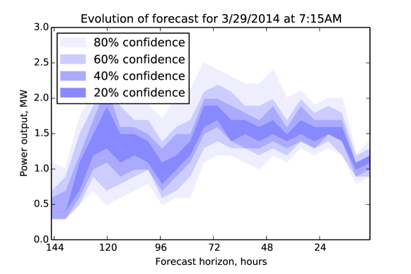
Figure 1: Evolution of the probabilistic forecast of power production of a wind plant as function of time, for a fixed production time.

In mathematical terms, let $(\Omega,\mathcal{F},\mathbb{F},\mathbb{P})$ be a filtered probability space and assume that $\mathbb{F}$ models the filtration of the decision maker. Fix a time horizon $T$, and let $X$ be a real-valued $\mathcal{F}_{T}$-measurable random variable. We make a standing assumption that $\mathcal{F}_{0}$ is a trivial $\sigma$-field. Let $\mu_{t}$ denote the regular conditional distribution of $X$ given $\mathcal{F}_{t}$. We call $\mu_{t}$ the probabilistic forecast of $X$ at time $t$. See [16] for the description of the mathematical framework of probabilistic forecasting and methods of forecast evaluation. The goal of this paper is to

• Formulate the conditions that the dynamics of $\mu_{t}$ must satisfy and propose several tractable finite-dimensional models for this dynamics in the diffusion framework,

• Show how these models may be calibrated with real meteorologic data, in the case where $\mu_{t}$ models the forecast of a meteorological variable.

• Provide an example of using the methodology to solve stochastic control problems arising in the context of wind energy trading.

The full predictive distribution is an infinite-dimensional object, but the actual available information is always low-dimensional; for this reason we aim to summarize the dynamics of the full predictive distribution with a low number of factors, which are easy to interpret and estimate from the data (such as the conditional mean and variance of the predictive distribution). In addition, our objective of computing the optimal strategies using the tools of stochastic control precludes the use of high-dimensional specifications. More precisely, in this paper we consider parametric two-dimensional specifications where the predictive distribution is a function of two observable factors, say $m_{t}$ and $V_{t}$. Here $m_{t}$ represents the conditional expectation of $X$ and $V_{t}$ some measure of the error, such as the conditional variance. In our models, $m_{t}$ and $V_{t}$ have diffusion dynamics, and the predictive density $\mu_{t}$ corresponds to a distribution from some known class, such as Student t, normal inverse Gaussian, inverse Gaussian or log generalized hyperbolic, with parameters depending on $m_{t}$ and $V_{t}$.

In practice, the forecast information received by the decision maker from a forecast provider may come, for example, in the form of a confidence interval around a point forecast, or in the form a set of quantiles of the predictive distribution. A particularly important case is that of ensemble forecasts. An ensemble forecast in meteorology is a set of several point forecasts aiming together to give an indication of the range of possible future states of the atmosphere. Members of the ensemble are obtained by running the forecasting model with perturbed initial conditions and / or parameters. An ensemble forecast is usually obtained with deterministic means, and therefore does not represent the best approximation of the predictive distribution of meteorological variables. In particular, ensemble forecasts are often uncalibrated (biased) and underdispersed compared to realizations [17]. However, techniques for statistical post-processing of ensemble forecast with the aim to improve calibration and sharpness have been developed in the literature. Two such techniques are ensemble model output statistics (EMOS) [17, 28] and Bayesian model averaging (BMA) [30, 25]. In [17], the authors approximate the predictive density with a Gaussian distribution, whose parameters depend on the ensemble forecasts and are chosen to optimize calibration and sharpness of the resulting probabilistic forecast. In [30, 25] the predictive density is reprensented by a mixture of normal distributions, whose weights are computed from the ensemble members. To account for positive random variables such as wind speed, EMOS with log-normal distributions has been used in [5] and BMA with truncated normal components has been employed in [4]. Other approaches to statistical post-processing of wind speed forecasts involve generalized extreme value distribution [21] and weighted mixtures of log-normal and truncated normal distributions [6].

In these papers, a single forecast horizon is fixed, and the calibration procedure uses a series of ensemble forecasts, obtained at different days of the training period for the fixed forecast horizon. At any given time, the calibrated method allows to compute the probabilistic forecast for this fixed horizon from the ensemble forecast, but no information about the evolution of the probabilistic forecast is available.

Our approach to calibrate the models presented in this paper is inspired by EMOS and also based on ensemble forecasts. However, we use more general predictive densities, potentially allowing for better calibration. More importantly, we do not fix a single forecast horizon, but model the dynamics of the predictive distribution for a given quantity at a given date, as time goes on and forecast horizon decreases. As a result, our calibrated model provides two types of information. First, as in statistical postprocessing methods, a predictive density in tractable form can be computed from an ensemble forecast. Secondly, the dynamics of this predictable distribution is given, in the form of a two-dimensional stochastic differential equation characterizing the evolution of the pair $(m_{t},V_{t})$, the conditional mean of the predictive distribution and a measure of the error. This dynamics can be exploited in the decision making process, to make strategy updates based not only on the conditional mean of the variable of interest, but also on the evolution of our knowledge of the uncertainty around the mean.

Stochastic differential equations (SDE) have been used to model the dynamics of probabilistic forecasts by several authors, see e.g., [18, 9] in the context of wind speed, or [3] in the context of solar energy forecasting. In these approaches, the forecasted quantity (e.g., the wind speed) is modeled directly by a stochastic differential equation, from which the probabilistic forecasts at any horizons, as well as their dynamics, can be deduced. However, the predictive distributions are typically not in tractable form (e.g., in [18] they are approximated by Monte Carlo), and the dynamics of the forecasting error is hard-coded into the equation and cannot be calibrated independently from ensemble forecasts, in other words, the variance of the forecast is not stochastic. This makes it impossible to use information on forecast uncertainty in strategy updates.

Our approach provides a dynamic SDE-based model for forecast dynamics, tractable predictive distribution and possibility of model calibration with ensemble forecasts, in a sense taking the best of both worlds to obtain a coherent and realistic model. Moreover, the results are exploited in a stochastic control problem to integrate the additional information provided by the probabilistic forecasts in the decision process.

Using probabilistic forecasts for decision making in wind energy trading and electricity scheduling has been studied e.g., in [23, 24, 31]. These references suggest a static approach, where a probabilistic forecast of a quantity of interest is used to make the decision on e.g., the quantity of energy to sell in the day-ahead market. By contrast, our dynamic approach allows to continuously, or regularly, update the decision based on the evolution of the forecast and information about its uncertainty.

We illustrate our methodological contribution with an application to a wind power trading problem. In this problem, a wind power producer, who disposes of a dynamically updated probabilistic forecast of the wind speed, takes positions in the intraday electricity market to maximize the utility of terminal wealth. This setting gives rise to a three-dimensional stochastic control problem, which is solved using the dynamic programming principle. For the numerical solution we use the Least Squares Monte Carlo method implemented in the open-source library StOpt (see [14]) and based on the methods of Bouchard and Warin [10] and Belomestny et al. [8] generalizing the seminal approach of Longstaff and Schwartz [22] and Tsitsiklis and Van Roy [29]. To assess the value of taking into account the dynamics of probabilistic forecasts, we compare the gains of an agent using our approach with the potential gains of another agent who uses only the point forecasts and show that our method leads to a 5% revenue increase in the simulation examples.

The paper is structured as follows. In section 2 we describe several parametric models for the dynamics of probabilistic forecasts. In section 3, we develop a procedure inspired by EMOS to calibrate the models of section 2 for different lead times and show that our models have good prediction results and that EMOS increases accuracy of prediction compared with raw ensembles, as expressed with Continuous Ranked Probability Score. In section 4, we present an application of our methodology to wind power trading.

2 Modeling probabilistic forecasts

As mentioned in the introduction, given a flow of information described by the filtration $(\mathcal{F}_{t})_{0\leq t\leq T}$, a probabilistic forecast of an $\mathcal{F}_{T}$-measurable random variable $X\in\mathbb{R}^{d}$ is the conditional distribution $\mu_{t}$ of $X$ given $\mathcal{F}_{t}$. A dynamic model for a probabilistic forecast is then a flow of probability measures $(\mu_{t})_{0\leq t\leq T}$, which can be identified with a flow of conditional distributions of some $\mathcal{F}_{T}$-measurable random variable. This imposes strong constraints on the dynamics of $(\mu_{t})$, in particular, all moments of $\mu_{t}$, when they exist, must be $(\mathcal{F}_{t})$-martingales. A $d$-dimensional Markov specification of forecast dynamics is a Markov process $(X_{t})_{0\leq t\leq T}\in\mathbb{R}^{d}$ such that, at every $t\in[0,T]$, $\mu_{t}=\mu(t,X_{t})$, where $\mu:[0,T]\to\mathbb{R}^{d}\to\mathcal{P}(\mathbb{R})$ is a deterministic mapping, where $\mathcal{P}(\mathbb{R})$ is the set of probability measures on $\mathbb{R}$.

In this section, we develop several two-dimensional Markov specifications for forecast dynamics, which correspond to well-known tractable predictive distributions.

2.1 Forecast of a real-valued quantity

In this section we propose two tractable models for the dynamics of probabilistic forecast of a real-valued quantity, such as the temperature. The models are based on the time-changed Brownian motion. In the first paragraph, the predictive distribution at all times is the Student t distribution (with power law tails), and in the second paragraph, the predictive distribution is the normal inverse Gaussian distribution (with exponentially decaying tails).

Student t predictive distribution

Let $\rho$ be a positive deterministic function, continuous on $(0,\infty)$, with $\int_{0}^{t}\rho^{2}(t)dt=+\infty$ for all $t>0$ (this function is singular at zero), let $W$ and $W^{\prime}$ be independent standard Brownian motions, whose filtration will be denoted by $\mathbb{F}$, let $b>0$ and consider the following pair of stochastic differential equations, defined for $t\in[0,T)$:

$$\frac{dV_{t}}{V_{t}} =-\rho^{2}(T-t)dt+b\rho(T-t)dW_{t}$$ (1)

$$dm_{t} =\sqrt{V_{t}}\rho(T-t)dW^{\prime}_{t},$$ (2)

Proposition 1.

The equation (1–2) admits a strong solution $(m,V)$ on $[0,T)$. The limit $m_{T}=\lim_{t\to T}m_{t}$ exists in the almost sure sense, and for every $t\in[0,T)$, the conditional distribution of $m_{T}$ given $\mathcal{F}_{t}$ is the Student t distribution with $2\nu$ degrees of freedom, where $\nu=1+2/b^{2}$:

$$\frac{d}{dx}\mathbb{P}[m_{T}\in dx|\mathcal{F}_{t}] =\frac{d}{dx}\mathbb{P}[m_{T}\in dx|m_{t},V_{t}]$$

$$=\frac{\Gamma(\nu+\frac{1}{2})}{\Gamma(\nu)}\frac{b}{2\sqrt{\pi V_{t}}}\left\{1+\frac{(x-m_{t})^{2}b^{2}}{4V_{t}}\right\}^{-\nu-\frac{1}{2}}.$$

In addition,

$$m_{t}=\mathbb{E}[m_{T}|\mathcal{F}_{t}]\quad\text{and}\quad V_{t}=\mathrm{Var}[m_{T}|\mathcal{F}_{t}].$$

Remark 1.

In this model, and in the other models of this section, the predictive distribution is parameterized by two (stochastic) variable parameters, $m_{t}$ and $V_{t}$ which typically determine the location and scale of the distribution and may change as time passes and the forecast horizon draws near, and one fixed parameter $b$ (typically, the shape parameter), which remains constant throughout the lifetime of the forecast for a fixed date. In addition, the deterministic time-varying parameter $\rho$ does not affect the predictive distribution, but affects the dynamics of the variables $m_{t}$ and $V_{t}$.

Remark 2.

The pair $(V_{t},m_{t})_{0\leq t<T}$ can alternatively be written as $V_{t}=\widetilde{V}_{\theta_{t}}$ and $m_{t}=\widetilde{m}_{\theta_{t}}$ with

$$\theta_{t}=\int_{0}^{t}\rho^{2}(T-s)ds,\quad 0\leq t<T,$$

and

$$\widetilde{V}_{t} =V_{0}e^{-(1+\frac{b^{2}}{2})t+b\widetilde{W}_{t}}$$

$$\widetilde{m}_{t} =m_{0}+\int_{0}^{t}\sqrt{\widetilde{V}_{s}}d\widetilde{W}^{\prime}_{s}$$

on $[0,\infty)$, with $(\widetilde{W},\widetilde{W}^{\prime})$ a standard $2$-dimensional Brownian motion.

Proof.

Fixing $t<T$, as in the above remark, for $s\geq t$, we can write

$$V_{s}=V_{t}\exp\left(-\int_{t}^{s}(1+b^{2}/2)\rho^{2}(T-u)du+\int_{t}^{s}b\rho(T-u)dW_{u}\right)=V_{t}\overline{V}^{(-1-b^{2}/2,b)}_{\int_{t}^{s}\rho(T-u)^{2}du}$$

where $\overline{V}^{(\mu,b)}_{t}=e^{\mu t+bB^{\prime}_{t}}$ for a different Brownian motion $B^{\prime}$. In addition,

$$\int_{t}^{T}\rho^{2}(T-s)V_{s}dt =V_{t}\int_{t}^{T}\rho^{2}(T-s)\overline{V}^{(-1-b^{2}/2,b)}_{\int_{t}^{s}\rho(T-u)^{2}du}ds=V_{t}\int_{0}^{\infty}\overline{V}^{(-1-b^{2}/2,b)}_{s}ds$$

$$=\frac{4V_{t}}{b^{2}}\int_{0}^{\infty}\overline{V}^{-(4/b^{2}-2,2)}_{s}ds.$$

From [12, Proposition 4.4.4],

$$\int_{0}^{\infty}\overline{V}_{t}^{(-4/b^{2}-2,2)}dt\stackrel{{\scriptstyle d}}{{=}}(2\gamma_{\nu})^{-1},\quad\nu=2/b^{2}+1,$$

where $\gamma_{\nu}$ denotes a gamma random variable with parameter $\nu$.

Then, for $t<s<T$,

$$m_{s}=m_{t}+B\left(\int_{t}^{s}V_{r}\rho^{2}(T-r)dr\right),$$

for a different Brownian motion $B$. Therefore,

$$m_{T}:=\lim_{s\to T}m_{s}=m_{t}+B\left(\int_{t}^{T}V_{r}\rho^{2}(T-r)dr\right)=B\left(\frac{2V_{t}}{b^{2}\gamma_{\nu}}\right)$$

and finally

$$\frac{d}{dx}\mathbb{P}[m_{T}-m_{t}\in dx|\mathcal{F}_{t}] =\mathbb{E}\left[\frac{b\sqrt{\gamma_{\nu}}}{2\sqrt{\pi V_{t}}}e^{-\frac{x^{2}b^{2}\gamma_{\nu}}{4V_{t}}}\right]$$

$$=\frac{b}{2\Gamma(\nu)\sqrt{\pi V_{t}}}\int_{0}^{\infty}e^{-z-\frac{x^{2}b^{2}z}{4V_{t}}}z^{\nu-\frac{1}{2}}dz$$

$$=\frac{\Gamma(\nu+\frac{1}{2})}{\Gamma(\nu)}\frac{b}{2\sqrt{\pi V_{t}}}\left\{1+\frac{x^{2}b^{2}}{4V_{t}}\right\}^{-\nu-\frac{1}{2}},$$

which means that conditionnally on $\mathcal{F}_{t}$, $m_{T}-m_{t}$ follows the centered Student t distribution with $2\nu=2+4/b^{2}$ degrees of freedom. The expressions for mean and variance are obtained from standard formulas for the Student t distribution. ∎

Figure 2 illustrates the dynamics of the predictive distribution in the model (1–2). We see that the confidence interval has a nontrivial behavior, it shrinks around the middle of the graph as the conditional variance goes down before increasing in size when the conditional variance goes up and shrinking to zero again at the very end.

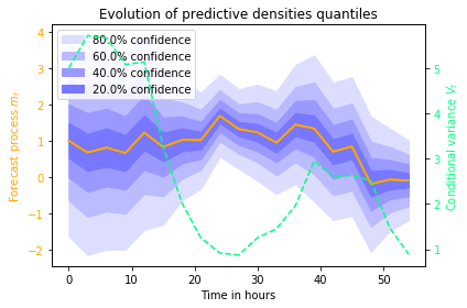
Figure 2: Confidence intervals for the Student predictive density, and the trajectories of the predictive distribution mean $m_{t}$ and variance $V_{t}$.

Normal inverse Gaussian predictive distribution

Using the notation of the previous paragraph, consider the following pair of stochastic differential equations.

$$dm_{t} =\sqrt{{V}_{t}}\rho(T-t)dW_{t}$$ (3)

$$d{V}_{t} =-{V}_{t}\rho^{2}(T-t)dt+\sqrt{{V}_{t}}b\rho(T-t)dW^{\prime}_{t}.$$ (4)

Here ${V}$ is a time-changed square-root process which hits zero in finite time almost surely. We assume that this process remains at zero after the first hitting time. A sample evolution of $(m,V)$ and the dynamics of the associated predictive distribution is shown in Figure 3. As in Remark 2, we can express $m_{t}=\widetilde{m}_{\theta_{t}}$ and ${V}_{t}=\widetilde{V}_{\theta_{t}}$, where the processes $\widetilde{m}$ and $\widetilde{V}$ have time-homogeneous dynamics (with different Brownian motions).

$${d\widetilde{m}_{t}} =\sqrt{\widetilde{V}_{t}}dW_{t}$$ (5)

$$d\widetilde{V}_{t} =-\widetilde{V}_{t}dt+\sqrt{\widetilde{V}_{t}}bdW^{\prime}_{t},$$ (6)

Proposition 2.

The equation (10–11) admits a strong solution $(m,V)$ on $[0,T)$. The limit $m_{T}=\lim_{t\to T}m_{t}$ exists in the almost sure sense, and for every $t\in[0,T)$, the conditional distribution of ${m_{T}}$ given $\mathcal{F}_{t}$ is the symmetric normal inverse Gaussian distribution on $\mathbb{R}$ with density

$$p(x)=\frac{\frac{{V}_{t}}{b^{2}}K_{1}\left(\frac{1}{b}\sqrt{({V}_{t}/b)^{2}+(x-m_{t})^{2}}\right)}{\pi\sqrt{({V}_{t}/b)^{2}+(x-m_{t})^{2}}}e^{{V}_{t}/b^{2}}$$ (7)

where $K$ is the modified Bessel function of the third kind. Moreover, the conditional mean and variance of $m_{T}$ are given by

$$m_{t}=\mathbb{E}[m_{T}|\mathcal{F}_{t}]\quad\text{and}\quad\mathrm{Var}\,[m_{T}|\mathcal{F}_{t}]={V}_{t}.$$

Proof.

For the existence of the strong solution to (5)–(6), see [19, Section 6.3.1] From Remark 2 it follows that for $s\geq\theta_{t}$,

$$\tilde{m}_{s}-m_{t}=\int_{\theta_{t}}^{s}\sqrt{\widetilde{V}_{u}}dW_{u}=\widetilde{W}_{\int_{\theta_{t}}^{s}\widetilde{V}_{u}du}$$

for a different Brownian motion $\widetilde{W}$. In particular

$$m_{T}=\widetilde{m}_{\infty}=m_{t}+\widetilde{W}_{\int_{\theta_{t}}^{\infty}\widetilde{V}_{s}ds}.$$

$\tilde{V}$ is a square root process with zero long-term mean. The Laplace transform of the integrated square root process is known [19, Proposition 6.3.4.1]:

$$\mathbb{E}\left[\exp\left(-u\int_{\theta_{t}}^{s}\widetilde{V}_{u}du\right)\Big{|}\widetilde{V}_{\theta_{t}}\right]=\exp\left(-\frac{2\widetilde{V}_{\theta_{t}}u}{1+\gamma\coth\frac{\gamma(s-\theta_{t})}{2}}\right),$$

where $\gamma=\sqrt{1+2ub^{2}}$. Integrating up to infinity, we then find:

$$\mathbb{E}\left[\exp\left(-u\int_{\theta_{t}}^{\infty}\widetilde{V}_{s}ds\right)\Big{|}\widetilde{V}_{\theta_{t}}\right]=\exp\left(-\frac{2\widetilde{V}_{\theta_{t}}u}{1+\sqrt{1+2ub^{2}}}\right).$$

This allows us to compute the Fourier transform of the conditional distribution of $m_{T}$:

$$\mathbb{E}[e^{iu({m_{T}}-{m_{t}})}|\mathcal{F}_{t}] =\mathbb{E}\left[\exp\left(iu\widetilde{W}_{\int_{\theta_{t}}^{\infty}\widetilde{V}_{s}ds}\right)|\widetilde{V}_{\theta_{t}}\right]$$

$$=\mathbb{E}\left[\exp\left(-\frac{u^{2}}{2}\int_{\theta_{t}}^{\infty}\widetilde{V}_{s}ds\right)\Big{|}\widetilde{V}_{\theta_{t}}\right]$$

$$=\exp\left(-\frac{\widetilde{V}_{\theta_{t}}u^{2}}{1+\sqrt{1+u^{2}b^{2}}}\right)$$

$$=\exp\left(-\frac{{V}_{t}(\sqrt{1+u^{2}b^{2}}-1)}{b^{2}}\right)$$

The characteristic function of the normal inverse Gaussian law with parameters $\mu$, $\alpha$, $\beta$, $\delta$ [7] is given by

$$e^{i\mu u+\delta(\sqrt{\alpha^{2}-\beta^{2}}-\sqrt{\alpha^{2}-(\beta+iu)^{2}})}.$$

Hence, $m_{T}-m_{t}$ conditionnally on $\mathcal{F}_{t}$ follows the normal inverse Gaussian law with parameters

$$\mu=0,\quad\delta=\frac{{V}_{t}}{b},\quad\beta=0,\quad\alpha=\frac{1}{b}.$$

The expressions of the conditional moments may be easily obtained from the characteristic function. ∎

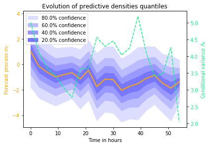
Figure 3: Confidence intervals for the NIG predictive density, and the trajectories of the predictive distribution mean $m_{t}$ and variance $V_{t}$.

2.2 Forecast of a positive quantity

In this section we propose two models for the probabilistic forecast of a positive quantity such as the wind speed. The models are obtained from the ones of the previous section, replacing the Brownian motion with the martingale geometric Brownian motion.

Log-generalized hyperbolic predictive distribution

Using the notation of the preceding section, consider the following pair of stochastic differential equations.

$$\frac{dV_{t}}{V_{t}} =-\rho^{2}(T-t)dt+b\rho(T-t)dW_{t}$$ (8)

$$\frac{dm_{t}}{m_{t}} =\sqrt{V_{t}}\rho(T-t)dW^{\prime}_{t}.$$ (9)

As in Remark 2, we can write $m_{t}=\widetilde{m}_{\theta_{t}}$ and ${V}_{t}=\widetilde{V}_{\theta_{t}}$, where the processes $\widetilde{m}$ and $\widetilde{V}$ have time-homogeneous dynamics (with different Brownian motions).

$$\frac{d\widetilde{m}_{t}}{\widetilde{m}_{t}} =\sqrt{\widetilde{V}_{t}}dW_{t}$$

$$\frac{d\widetilde{V}_{t}}{\widetilde{V}_{t}} =-dt+bdW^{\prime}_{t}.$$

Proposition 3.

Let $(m,V)$ be a solution of (8–9). Then the conditional distribution of $\log m_{T}$ given $\mathcal{F}_{t}$ is the generalized hyperbolic distribution with density

$$p(x)=\frac{be^{\frac{x-\mu}{2}}}{\Gamma(\nu)\sqrt{\pi V_{t}}}\left(\frac{V_{t}}{b\sqrt{4V_{t}+(x-\mu)^{2}b^{2}}}\right)^{\nu+\frac{1}{2}}K_{\nu+\frac{1}{2}}\left(\sqrt{\frac{V_{t}}{b^{2}}+\frac{(x-\mu)^{2}}{4}}\right)$$

with $\mu=\log m_{t}$ and $\nu=1+\frac{2}{b^{2}}$. In addition,

$$\mathbb{E}[m_{T}|\mathcal{F}_{t}]=m_{t}.$$

Remark 3.

This distribution is a particular case of the generalized hyperbolic distribution, known as generalized hyperbolic skew Student t distribution [1]. With this distribution, $m_{T}$ does not admit a second moment.

Proof.

With the notation of the proof of Proposition 1, we now get

$$\log\frac{m_{T}}{m_{t}}=W\left(\frac{2V_{t}}{b^{2}\gamma_{\nu}}\right)-\frac{V_{t}}{b^{2}\gamma_{\nu}},$$

and therefore

$$\frac{d}{dx}\mathbb{P}[\log(m_{T}/m_{t})\in dx|\mathcal{F}_{t}] =\frac{d}{dx}\mathbb{E}[\mathbb{P}[\log(m_{T}/m_{t})\in dx|\gamma_{\mu},V_{t}]]$$

$$=\mathbb{E}\left[\frac{b\sqrt{\gamma_{\mu}}}{2\sqrt{\pi V_{t}}}e^{-\frac{(x-\frac{V_{t}}{b^{2}\gamma_{\mu}})^{2}b^{2}\gamma_{\mu}}{4V_{t}}}\right]$$

$$=\frac{be^{\frac{x}{2}}}{2\Gamma(\mu)\sqrt{\pi V_{t}}}\int_{0}^{\infty}e^{-z\left(1+\frac{x^{2}b^{2}}{4V_{t}}\right)-\frac{V_{t}}{4b^{2}z}}z^{\mu-\frac{1}{2}}dz$$

$$=\frac{be^{\frac{x}{2}}}{\Gamma(\mu)\sqrt{\pi V_{t}}}\left(\frac{V_{t}}{b\sqrt{4V_{t}+x^{2}b^{2}}}\right)^{\mu+\frac{1}{2}}K_{\mu+\frac{1}{2}}\left(\sqrt{\frac{V_{t}}{b^{2}}+\frac{x^{2}}{4}}\right).$$

∎

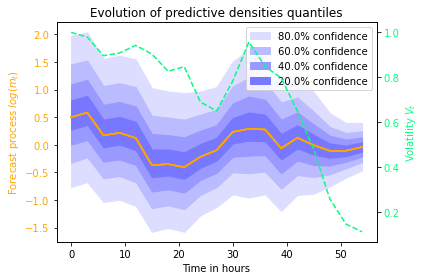
Figure 4: Confidence intervals for the log-generalized hyperbolic predictive density and the trajectories of the processes $m$ and ${V}$

Log-normal inverse Gaussian predictable distribution

Using the same notation as above, consider the following pair of SDEs.

$$\frac{dm_{t}}{m_{t}} =\sqrt{V_{t}}\rho(T-t)dW_{t}$$ (10)

$$dV_{t} =-V_{t}\rho^{2}(T-t)\left(1+\frac{b^{2}}{2}\right)dt+\sqrt{V_{t}}b\rho(T-t)dW^{\prime}_{t}.$$ (11)

The equivalent time-changed representation takes the form

$$\frac{d\widetilde{m}_{t}}{\widetilde{m}_{t}} =\sqrt{\widetilde{V}_{t}}dW_{t}$$ (12)

$$d\widetilde{V}_{t} =-\widetilde{V}_{t}\left(1+\frac{b^{2}}{2}\right)dt+\sqrt{\widetilde{V}_{t}}bdW^{\prime}_{t}.$$ (13)

The proof of the following proposition is very similar to that of Proposition 2 and will therefore be omitted.

Proposition 4.

Let $(m,V)$ be a solution of (10–11). Then the conditional distribution of $\log{m_{T}}$ given $\mathcal{F}_{t}$ is the normal inverse Gaussian distribution on $\mathbb{R}$ with density

$$p(x)=\frac{\alpha\delta K_{1}\left(\alpha\sqrt{\delta^{2}+(x-\mu)^{2}}\right)}{\pi\sqrt{\delta^{2}+(x-\mu)^{2}}}e^{\delta\gamma+\beta(x-\mu)}$$ (14)

where the parameters are given by

$$\mu=\log m_{t},\quad\delta=\frac{V_{t}}{b},\quad\beta=-\frac{1}{2},\quad\alpha=\sqrt{(b^{-1}+\frac{b}{2})^{2}+\frac{1}{4}},$$

$\gamma=b^{-1}+\frac{b}{2}$, and $K$ is the modified Bessel function of the third kind. Moreover, the first two conditional moments of $m_{T}$ are given by

$$m_{t}=\mathbb{E}[m_{T}|\mathcal{F}_{t}]\quad\text{and}\quad\mathbb{E}[m_{T}^{2}|\mathcal{F}_{t}]=m_{t}^{2}e^{V_{t}}.$$

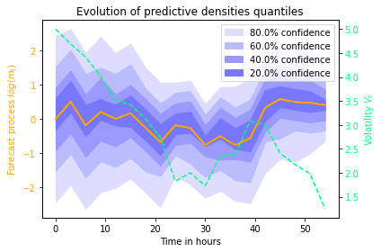
Figure 5: Confidence intervals for the log normal inverse Gaussian predictive density and the trajectories of the processes $m$ and $V$.

Note that for all processes presented in this section, the process $V_{t}$ does not necessarily decrease with time (see Figures 2-5). This reflects the fact that uncertainty over the quantity to forecast can vary over time and does not always decrease as we approach the realization date. We also attract the reader’s attention on the fact that while $V_{t}$ does represent the forecast uncertainty, it does not coincide with the conditional variance of the predictive density for positive quantities – e.g., for $(m,V)$ solution of (10)–(11), the variance is given by $\text{Var}[m_{T}|\mathcal{F}_{t}]=m^{2}_{t}(e^{V_{t}}-1)$.

3 Fitting forecast models to data

In this section, we detail the procedure for calibrating our models for forecast dynamics from historical ensemble forecasts and the corresponding realizations. To illustrate the forecasting of a real-valued quantity, we shall use the normal inverse Gaussian model defined by the equations (3–4) and the predictive density (7), and apply it to ensemble forecasts of temperature. To ilustrate the forecasting of a positive quantity, we shall use the model defined by the equations (10–11) and the predictive density (14), and apply it to ensemble forecasts of the wind speed.

3.1 Presentation of the dataset

The data is composed of meteorological ensemble forecasts from $K=273$ different locations around Paris, France, plotted on the map in Figure 6, recorded over January 2015.

Figure 6: Locations of the meteorological records

A new forecast ensemble becomes available at 12PM (noon) and at 12AM (midnight) on each day. Each forecast ensemble consists of 50 members, and each member provides a prediction for all meteorological variables for lead times from 1h to 48h, with a step of 3h. Since the forecasts are updated every 12 hours, in our study of forecasts dynamics, we use only the forecast horizons which are multiples of 12 hours, that is, $h\in\mathcal{H}=\{12,24,36,48\}$.

As the locations are very close to each other we make the approximation that they form several ensemble forecasts of the same area. We will use all the ensemble forecasts to calibrate the model, making the approximation that, for each time horizon, the calibrated coefficient can be used to obtain the predictive densities in each of these locations.

Forecasts recorded on days from January 3 to January 21 constitute the training set and those recorded from January 22 to January 31 form the test set.

Note that the first two days of January are not used for the calibration because we do not dispose of the full forecast data for them. Our training set is thus composed of $T=38$ 12-hour periods.

In this application we are interested in two variables: the temperature at 2 meter height denoted by $\tau$ and the 10 meter wind speed denoted by $w$. The wind speed is not directly available in the data and we compute it from the two components $w_{x}$ and $w_{y}$ through the usual formula $w=\sqrt{w_{x}^{2}+w_{y}^{2}}$ for each member of the forecast ensemble and for each realization.

Since the maximum lead time for our forecast is 48 hours and new forecast becomes available every 12 hours, to study the dynamics of the forecast of a given realization recorded at 12 AM or 12 PM, we dispose of 4 data points with lead times 48h, 36h, 24h and 12h. In Figure 7, we plot four forecast ensembles for the wind speed, recorded for a specific location in our dataset at four consecutive forecast update times (Jan 1st 12PM, Jan 2nd 12AM, Jan 2nd 12 PM and Jan 3rd 12AM). The forecasts for a fixed terminal time (Jan 3rd, 12 PM) are shown with the vertical bar in the four graphs.

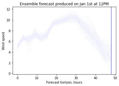
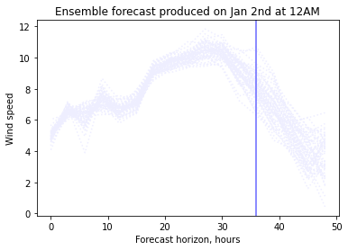
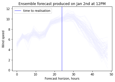
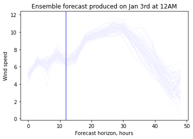
Figure 7: Forecast ensembles for the wind speed, recorded at four consecutive forecast update times (Jan 1st 12PM, Jan 2nd 12AM, Jan 2nd 12 PM and Jan 3rd 12AM). The forecasts for a fixed terminal time (Jan 3rd, 12 PM) are shown with the vertical bar

3.2 Model calibration

To calibrate our models for forecast dynamics from meteorological ensemble forecasts, we use an approach inspired by the EMOS methodology in [17], to determine the conditional mean and variance of the predictive distribution from the ensemble forecasts. As explained in the introduction, the ensemble forecasts may be biased and underdispersed, so that the mean and variance of the predictive distribution are not necessarily equal to the mean and variance of the empirical distribution of the forecast members, although these quantities are certainly related to each other. Let $x^{m}_{htk}$ denote the value of member $m$ of the ensemble forecast of a given meteorological quantity (wind speed or temperature), recorded at time $t$, at location $k$, for the forecast horizon $h$, and by $\tilde{x}_{tk}$ the corresponding realization. We assume that the mean of the predictive distribution, denoted by $m_{htk}$ is a linear function of the mean of ensemble members:

$$m_{htk}=m_{htk}(a^{0}_{h},a^{1}_{h})=a^{0}_{h}+\frac{a^{1}_{h}}{M}\sum_{m=1}^{M}x^{m}_{htk}:=a^{0}_{h}+a^{1}_{h}\bar{x}_{htk}.$$ (15)

The coefficients $a^{0}_{h}$ and $a^{1}_{h}$ reflect the bias in the ensemble forecasts. In the case of unbiased forecasts we would have $a^{0}_{h}=0$ and $a^{1}_{h}=1$. Similarly, the variance of the predictive distribution depends on the spread of ensemble members, but the latter may not reflect the forecasting error entirely. Hence we assume that at each date $t$, each location $k$, and each lead time $h$, the variance of the predictive distribution is given by

$$\sigma^{2}_{htk}=\sigma^{2}_{htk}(c_{h},d_{h})=c_{h}+d_{h}\frac{1}{M}\sum_{m=1}^{M}(x^{m}_{htk}-\bar{x}_{htk})^{2}:=c_{h}+d_{h}V_{htk}.$$ (16)

The coefficients in the expression for the variance can be interpreted as follows: $c_{h}$ represents the part of the error that is not related to the spread of the ensemble members, whereas $d_{h}$ represents the part of the conditional variance explained by the ensemble spread.

The full model specification for the temperature forecasts is thus given by equations (3–7) and (15–16), while the full specification for the wind forecasts is given by equations (10–14) and (15–16).

The full model is calibrated in a three-step procedure as detailed below.

Step 1

In the first step, we first calibrate, separately for each forecast horizon, the parameters $a^{0}_{h}$ and $a^{1}_{h}$ by linear regression:

$$(\hat{a}_{h}^{0},\hat{a}_{h}^{1})=\underset{a^{0},a^{1}}{\arg\min}\sum_{t,k=1}^{T,K}(a^{0}+a^{1}\bar{x}_{htk}-\tilde{x}_{tk})^{2}.$$

Next, using the calibrated values $\hat{a}_{h}^{0}$ and $\hat{a}_{h}^{1}$, we calibrate $c_{h}$, $d_{h}$ and $b_{h}$ by maximum likelihood:

$$(\hat{c}_{h},\hat{d}_{h},\hat{b}_{h})=\underset{c,d,b}{\arg\max}\sum_{t,k=1}^{T,K}\log p(\tilde{x}_{tk},m_{htk}(\hat{a}_{h}^{0},\hat{a}_{h}^{1}),\sigma^{2}_{htk}(c,d),b),$$

where $p(x,m,\sigma^{2},b)$ denotes the predictive density expressed in terms of the conditional mean $m$, the conditional variance $\sigma^{2}$ and the shape parameter $b$.

For the temperature, the predictive density (7) writes,

$$p^{\tau}(x,m,\sigma^{2},b)=\frac{\frac{\sigma^{2}}{b^{2}}K_{1}\left(\frac{1}{b}\sqrt{(\sigma^{2}/b)^{2}+(x-m)^{2}}\right)}{\pi\sqrt{(\sigma^{2}/b)^{2}+(x-m)^{2}}}e^{\sigma^{2}/b^{2}},$$

and for the wind speed, the predictive density (14) writes,

$$p^{w}(x,m,\sigma^{2},b)=\frac{\alpha VK_{1}\left(\frac{\alpha}{b}\sqrt{V^{2}+b^{2}(x-\log m)^{2}}\right)}{\pi\sqrt{V^{2}+b^{2}(x-\log m)^{2}}}e^{V(b^{-2}+\frac{1}{2})-\frac{1}{2}(x-\log m)}$$

where

$$\alpha=\sqrt{(b^{-1}+\frac{b}{2})^{2}+\frac{1}{4}}\quad\text{and}\quad V=\log\left(\frac{\sigma^{2}}{m^{2}}+1\right).$$

Note that in this step, the shape parameter $b_{h}$ is calibrated independently for each forecast horizon. A common value for all horizons will be fixed in the next step. The choice of the maximum likelihood procedure in this first step was motivated by the availability of predictive densities in explicit form. An alternative would be to use the Continuous Ranked Probability Score (CRPS) as in [17], but for our models the CRPS is only available through heavy numerical computation, making the approach of [17] difficult to implement. We also tested direct maximum likelihood estimation of the four parameters $a^{0}_{h},a^{1}_{h},c_{h},d_{h}$ and $b_{h}$, but the presented approach where linear regression is used for $a^{0}_{h},a^{1}_{h}$ leads to better results.

Step 2

In the previous step, the shape parameter $b$ was calibrated separately for each lead time. However, in our model, this parameter does not depend on the forecast lead time. Thus, once the parameters $a^{0}_{t},a^{1}_{t},c_{t},d_{t}$ have been estimated in the first step, we perform again an estimation of the parameter $b$ by maximizing the likelihood including all forecast horizons:

$$\hat{b}=\underset{b}{\text{argmax}}\sum_{h\in\mathcal{H}}\sum_{t,k=1}^{T,K}\log p(\tilde{x}_{tk},m_{htk}(\hat{a}_{h}^{0},\hat{a}_{h}^{1}),\sigma^{2}_{htk}(\hat{c}_{h},\hat{d}_{h}),b).$$

This formulation applies for both the temperature and the wind speed calibration. This procedure does not impact the goodness of fit in terms of first and second moment since the parameters of the mean and the variance are fixed. However, the shape of the distribution may change a bit with no major impact.

Step 3

Once we have estimated the ’static’ properties of the model, that is, the parameters which appear in the predictive distribution ($b$ and $a_{0}$, $a_{1}$, $c$ and $d$ for each time horizon), we need to estimate the ’dynamic parameter’, that is, the function $\rho$, which describes how the forecast varies dynamically. While the static parameters are estimated by comparing the forecasts with their respective realizations, $\rho$ can be estimated by comparing forecasts for the same quantity, obtained at different dates.

For the temperature model, from equation (4), we may write:

$$\mathbb{E}\left[\frac{V_{t+s}}{V_{t}}|\mathcal{F}_{t}\right]=\exp{\left(-\int_{t}^{t+s}\rho(T-u)^{2}du\right)}.$$

Since the expectation in the right-hand side is deterministic, we can remove the conditioning and write:

$$\int_{t}^{t+s}\rho(T-u)^{2}du=-\log\left(\mathbb{E}\left[\frac{V_{t+s}}{V_{t}}\right]\right)$$ (17)

Based on this identity, we suggest the following approach to calibrate $\rho$ based on a given discrete set of forecast horizons $0<h_{1}<\dots<h_{H}=T$, for which data are available. Here $h_{H}$ corresponds to the longest available horizon (when the simulation starts) and $h_{1}$ corresponds to the shortest available horizon (last available forecast for a given realization). Assume that $\rho$ is constant on the intervals $(h_{i},h_{i+1})$, $i=1,\dots,H-1$ and denote the value of $\rho$ on the interval $(h_{i},h_{i+1})$ by $\rho_{i}$. This assumption is without loss of generality since, in view of Equations (5–6) and (12–13), the law of $(m_{h_{i+1}},V_{h_{i+1}})$ conditional on $(m_{h_{i}},V_{h_{i}})$ depends on $\rho$ only through the integral $\int_{h_{i}}^{h_{i+1}}\rho(T-u)^{2}du$.

In view of (17), we propose to estimate the values $\rho_{1},\dots,\rho_{H-1}$ as follows:

$$\hat{\rho}^{2}_{i}=-\frac{1}{(h_{i+1}-h_{i})}\log\frac{1}{TK}\sum_{t,k=1}^{T,K}\frac{\sigma^{2}_{h_{i+1}tk}(\hat{c}_{h_{i+1}},\hat{d}_{h_{i+1}})}{\sigma^{2}_{h_{i}tk}(\hat{c}_{h_{i}},\hat{d}_{h_{i}})}.$$

For the wind speed model, from equations (10-11), we may write:

$$\mathbb{E}\left[\log\frac{m_{t+h}}{m_{t}}|\mathcal{F}_{t}\right]=-\frac{1}{2}\int_{t}^{t+h}\rho^{2}(T-s)\mathbb{E}[V_{s}|\mathcal{F}_{t}]ds,$$

and

$$\mathbb{E}[V_{s}|\mathcal{F}_{t}]=V_{t}\exp\left(-\left(1+\frac{b^{2}}{2}\right)\int_{t}^{s}\rho^{2}(T-u)du\right),$$

so that

$$\mathbb{E}\left[\log\frac{m_{t+h}}{m_{t}}|\mathcal{F}_{t}\right]=-\frac{V_{t}}{2+b^{2}}\left(1-\exp\left(-\left(1+\frac{b^{2}}{2}\right)\int_{t}^{t+h}\rho^{2}(T-u)du\right)\right).$$

Dividing both sides by $V_{t}$, we can remove the conditioning and rewrite this expression as follows:

$$\int_{t}^{t+h}\rho^{2}(T-u)du=-\frac{2}{2+b^{2}}\log\left(1+(2+b^{2})\mathbb{E}\left[\frac{1}{V_{t}}\log\frac{m_{t+h}}{m_{t}}\right]\right).$$

As before, assume without loss of generality that $\rho$ is constant on every interval $(h_{i},h_{i+1})$ for $i=1,\dots,H-1$, and denote its value on such interval by $\rho_{i}$. This suggests the following estimator for $\rho_{i}$:

$$\hat{\rho}_{i}=-\frac{1}{h_{i+1}-h_{i}}\frac{2}{2+\hat{b}^{2}}\log\left(1+(2+\hat{b}^{2})\frac{1}{TK}\sum_{t,k=1}^{T,K}\frac{1}{\sigma^{2}_{h_{i}tk}(\hat{c}_{h_{i}},\hat{d}_{h_{i}})}\log\frac{m_{t+h}}{m_{t}}\right).$$

3.3 Numerical illustrations

In this section we apply the methodology presented in section 3.2 to ensemble forecasts for the wind speed and the temperature described in 3.1.

Estimated coefficients

As explained in section 3.2, we use an EMOS-inspired technique to improve the calibration of ensemble forecasts. To motivate this post-processing, we present in Figure 8 the Talagrand diagrams (rank histograms) for the ensemble forecasts of the log wind speed and the temperature, constructed using the test data. Talagrand diagram is a tool for checking the quality of calibration of ensemble forecasts and is a histogram of the ranks of observations within the corresponding forecast ensembles. In other words, for a given forecast horizon $h$, we plot the histogram of $R(\tilde{x}_{tk},(x_{htk}^{m})_{m=1\dots M})_{t,k=1}^{T,K}$, where $R(\tilde{x},(x^{m})_{m=1\dots M})$ is the normalized rank of the observation $\tilde{x}$ within the ensemble $(x^{m})_{m=1\dots M}$. For a perfectly calibrated ensemble forecast, the Talagrand diagram is within the confidence bounds of the uniform distribution. In the present case, histograms in Figure 8, for the lead time $12h00$, and Figure 9, for the lead time $24h00$, present a U-shaped profile, which is a clear indication of under-dispersion of our forecast ensembles. In addition, the asymmetric form of the diagram for the wind speed in Figure 8, and for the temperature in Figure 9, is an indication of the presence of a bias in the ensemble forecast. Histograms for lead times $36h00$ and $48h00$ are available in Appendix 4.3.

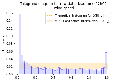
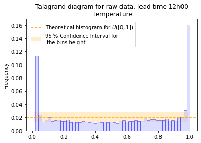
Figure 8: Talagrand diagrams for the wind speed and the temperature, lead time $12h00$

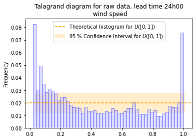
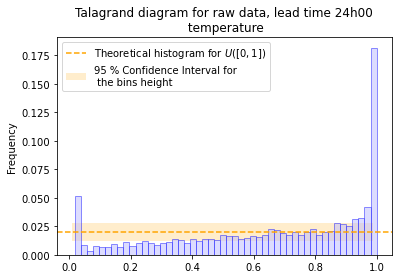
Figure 9: Talagrand diagrams for the wind speed and the temperature, lead time $24h00$

In view of the Talagrand diagrams discussed above, we apply our post-processig approach to obtain an unbiased and well-calibrated probabilistic forecast. Tables 1 and 2 show, respectively, the estimated coefficients for the wind speed and the temperature during the training period.

Lead time	$a^{0}$	$a^{1}$	$c$	$d$	$b$
12h	0.117	0.964	0.360	0.765	0.035
24h	-0.028	0.994	0.446	0.494	0.035
36h	-0.083	1.006	0.951	0.160	0.035
48h	-0.573	1.044	0.240	0.798	0.035

Lead time	$\rho(.)$
interval
12h-24h	0.171
24h-36h	0.153
36h-48h	0.168

Table 1: Calibrated coefficients for the wind speed from the 1^st to the 21^th of January 2015

Lead time	$a^{0}$	$a^{1}$	c	d	b
12h	0.217	0.952	0.312	1.722	0.719
24h	0.103	1.006	0.416	0.916	0.719
36h	0.136	1.019	0.675	0.467	0.719
48h	0.202	1.015	0.306	0.913	0.719

Lead time	$\rho(.)$
interval
12h-24h	0.160
24h-36h	0.163
36h-48h	0.180

Table 2: Calibrated coefficients for the temperature from the 1^st to the 21^th of January 2015

The spread coefficients $c$ and $d$ confirm that the raw ensemble forecasts are underdispersed: except for the $24h$ lead time wind speed forecasts, all provide a post process variance larger than the ensemble forecast spread. This is especially true for the $12h$ lead time temperature forecast which has an intercept of $c=0.312$ and a slope of $d=1.772$ which multiply almost by two the original variance.

We now proceed to analyse the diffusion coefficients $b$ and $\rho$. The parameter $b$ is quite low for the log wind speed distribution. This suggests that the log-wind speed distribution is closer to the Gaussian one, than the temperature distribution for which the coefficient $b$ is higher. This indicates a heavier tailed model where extreme temperature values are more likely to happen than extreme wind spikes.

The values of the piecewise constant function $\rho(.)$ are very close to each other on the three time intervals considered for both the wind speed and the temperature. This feature will be useful when using this dynamics in the control problems in section 4.

Goodness of fit

In this paragraph, we check the goodness of fit of the estimated predictive distribution using the test dataset and provide some illustrations. We first present the mean square error computed using the test data before and after the pre-processing that is :

$$\text{MSE}^{\text{raw}}(h)=\sum_{t,k=1}^{T,K}(\bar{x}_{htk}-\tilde{x}_{tk})^{2},\quad\text{MSE}(h)=\sum_{t,k=1}^{T,K}(a^{0}_{h}+a^{1}_{h}\bar{x}_{htk}-\tilde{x}_{tk})^{2}.$$

Except for the wind speed at lead times $36h$ and $48h$, the correction of the bias brings the mean of the test data closer to the realization. Hence our estimation procedure doesn’t overfit the training period and is robust when considering new data. However, we should mention that this is done over data for the same month and the same season. We may assume that the seasonality impacts the value of the coefficients and repeating the study over different months may provide additional insights.

Log wind speed
Lead time	MSE	MSE
	Raw ensemble	Model
12h	0.948	0.804
24h	0.955	0.931
36h	1.233	1.240
48h	1.633	1.795

Temperature
Lead time	MSE	MSE
	Raw ensemble	Model
12h	0.656	0.599
24h	0.851	0.778
36h	0.973	0.900
48h	1.539	1.424

Table 3: MSE for the log wind speed and the temperature over the period (22/01-31/01)

To evaluate the calibration of the predictive distribution we use the probability integral transform (PIT) histogram and to check both calibration and sharpness, we compute the continuous rank probability score (CRPS). The formal definition of the CRPS for a given realisation $y$ and a predictive distribution with cumulative distribution function (CDF) $F$ is given by:

$$\text{CRPS}(F,y)=\int_{\mathbb{R}}(F(x)-\mathbbm{1}_{\{y\leq x\}})^{2}dx$$

For the normal inverve Gaussian and the log normal inverse Gaussian distributions, it is not possible to compute the analytical expression of the CDF. However, we can use the Plancherel formula and obtain an expression relying on the characteristic function $\phi$ of the normal inverse Gaussian predictive distribution:

$$\int_{\mathbb{R}}(F(x)-\mathbf{1}_{y\leq x})^{2}dx =\frac{1}{2\pi}\int_{\mathbb{R}}\frac{|\phi(u)-e^{iuy}|^{2}}{u^{2}}du$$

$$=\frac{1}{2\pi}\int_{\mathbb{R}}\frac{\Big{|}e^{i\mu u+\delta\left(\gamma-\sqrt{\alpha^{2}-(\beta+iu)^{2}}\right)}-e^{iuy}\Big{|}^{2}}{u^{2}}du,$$

Following this formulation, for a predictive distribution for the location $k$, the lead time $h$ and the date $t$, we denote the CDF $F_{tkh}$ and the realisation $y_{tkh}$. The parameters $\alpha,\beta,\gamma,\delta$ and $\mu$ for temperature are given by,

$$\alpha=\frac{1}{b},\;\beta=0,\;\gamma=\frac{1}{b},\;\delta=\frac{V_{htk}}{b},\;\mu=m_{htk},$$

and for the wind speed:

$$\alpha=\sqrt{\left(\frac{1}{b}+\frac{b}{2}\right)^{2}+\frac{1}{4}},\;\beta=-\frac{1}{2},\;\gamma=\frac{1}{b}+\frac{b}{2},\;\delta=\frac{V_{htk}}{b},\;\mu=\log(m_{htk}).$$

We analyse the goodness of fit using the averaged CRPS over the period 22/01/15-31/01/15 for each lead time,

$$\text{averageCRPS}_{h}(F,y)=\frac{1}{TK}\sum_{t,k=1}^{T,K}\int_{\mathbb{R}}\left(F_{tkh}(x)-\mathbbm{1}_{\{y_{tkh}\leq x\}}\right)^{2}dx$$

We compare it to the averaged CRPS obtained with the raw ensemble forecasts, that is:

$$\text{averageCRPS}_{h}(\text{Ensemble forecasts},y_{tkh})=\frac{1}{TK}\sum_{t,k=1}^{T,K}\int_{\mathbb{R}}\left(\hat{F}^{M}_{tkh}(x)-\mathbbm{1}_{\{y_{tkh}\leq x\}}\right)^{2}dx,$$

where

$$\hat{F}^{M}_{tkh}(x)=\frac{1}{M}\sum_{m=1}^{M}\mathbf{1}_{\{x^{m}_{tkh}\leq x\}}$$

and for each location, date and lead time, we may simplify the CRPS formula as follows:

$$\text{CRPS}(\hat{F}^{M}_{tkh},y_{tkh}) =\int_{\mathbb{R}}\left(\hat{F}^{M}_{tkh}(x)-\mathbbm{1}_{\{y_{tkh}\leq x\}}\right)^{2}dx$$

$$=\frac{2}{M}\sum_{\ell=1}^{M}(x_{(\ell)}-y_{tkh})\left\{\mathbf{1}_{\{x_{(\ell)}>y_{tkh}\}}-\frac{\ell-\frac{1}{2}}{M}\right\},$$

where $x_{(\ell)},k=1\dots M$ is the order statistics of the sample $x^{m}_{tkh},m=1\dots M$.

Table 4: CPRS for the wind speed ($\log m.s^{-1}$) and for the temperature (C$\degree$) over the test period 22/01/15-31/01/15

log wind speed
Lead time	12h	24h	36h	48h
EMOS	0.039	0.056	0.062	0.128
Raw	0.080	0.095	0.100	0.102

temperature
Lead time	12h	24h	36h	48h
EMOS	0.372	0.437	0.485	0.639
Raw	0.450	0.481	0.538	0.752

Table 4 compares the CRPS computed using the test period for raw ensemble forecast and for probabilistic forecasts obtained using our post-processing method. We observe a significant improvement for both wind speed and temperature forecasts, for all forecast horizons except the 48-hour forecast horizon for the wind speed.

As an independent illustration of the calibration of the post-processed forecasts we plot the probability integral transforms (PIT), which is the equivalent of Talagrand diagram in the context of probabilistic forecasts and consists in plotting the histogram of the predictive CDF evaluated at the realization point. If the predictive distribution is well calibrated then the histogram should be close to the uniform one.

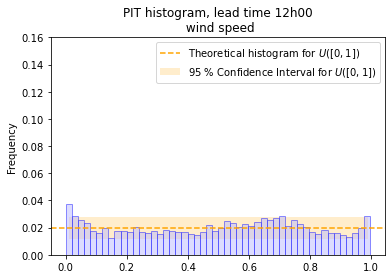
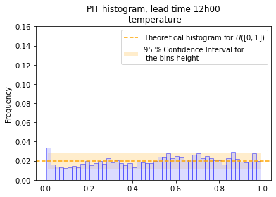
Figure 10: PIT histogram for the wind speed and the temperature, lead time $12h00$

The PIT of post-processed forecasts are shown in Figures 10 and 11 and may be compared to Talagrand diagrams in Figures 8–9. Here again, the improvement is considerable, although some deviations from the uniform distribution can still be observed. They may be explained by the fact that we use a parametric approach, which obviously cannot provide a perfect fit to the data, and our observations are not completely independent.

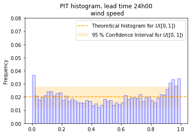
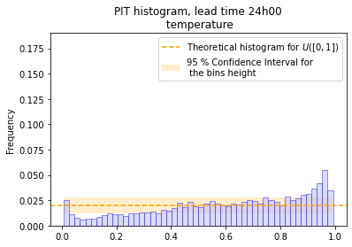
Figure 11: PIT histogram for the wind speed and the temperature, lead time $24h00$

Behavior of the predictive density in test data

To illustrate the shape of the predictive density obtained with our approach, we displayed in Figure 12, for a given realization date (22/01/15 at 12 a.m) and location, the predictive densities at each lead time as well as the realisation for the wind speed forecasts. We observe that the sharpness of the predictive distribution varies with the lead time. Interestingly it doesn’t always improve as we approach the realisation time (e.g see the temperature predictive densities at lead times $12h$ and $24h$). This is to be compared with the simulated predictive distributions in Figures 5 and 3.

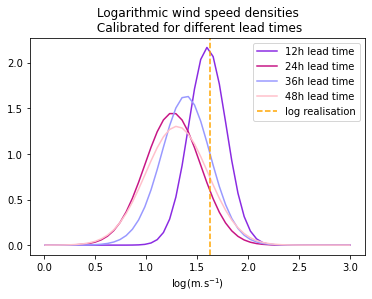
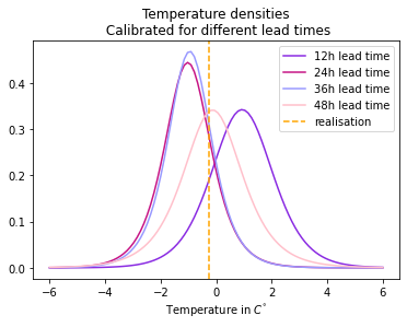
Figure 12: Example of predictive densities produced by the model

At the same location we plotted the evolution of the point forecast (first moment of the predictive distribution) for a fixed lead time and the corresponding realization over the period 22/01/15-31/01/15 in Figure 13. We also show the confidence intervals around the point forecast. The realization always falls in the 90 $\%$ confidence interval and the width of the intervals varies throughout the simulation. The forecasts seem reasonably close to the realizations: this is especially true when the width of the confidence interval is small.

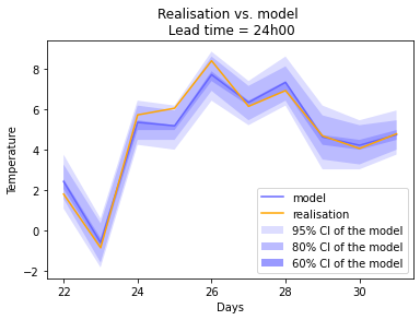
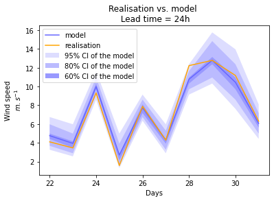
Figure 13: Temperature and wind speed forecasts for the period 22/01/2015-31/01/2015

Table 6 shows the average width of the 90 $\%$ confidence interval, for the testing period: 22/01/2015-31/01/2015. For the first three lead times the width increases with lead time but the 36h lead time confidence intervals are on average sightly larger than the 48 h lead time ones. This confirms the intuition that the closer we get to the realisation date the less variations there are in forecasts updates (on average). On the other hand, finding a wider confidence interval average for the lead time $36h$ than for the lead time $48h$ is quite unexpected. We investigated the confidence interval width during the training period in Table 5 and found that the confidence interval width always decreases as we approach the realization time. This suggests that the model may not be fully consistent with the test data, perhaps owing to a possible non-stationarity of the forecasts.

Lead time	90$\%$ CI width	90$\%$ CI width
	Wind speed	Temperature
12h	2.565	2.605
24h	2.869	2.923
36h	3.381	3.301
48h	3.628	3.585

Table 5: Average 90 $\%$ confidence interval for the period 01/01-21/01 for the wind speed and the temperature

Lead time	90$\%$ CI width	90$\%$ CI width
	Wind speed	Temperature
12h	2.537	2.592
24h	2.801	2.747
36h	3.378	3.062
48h	3.254	2.956

Table 6: Average 90 $\%$ confidence interval for the period 22/01-31/01 for the wind speed and the temperature

4 Application to wind power trading

In this section we present an application of our methodology based on the dynamic modeling of probabilistic forecasts to the problem of wind power trading in the intraday electricity market.

4.1 Description of the problem

Consider a wind power producer who aims to sell the output power in the intraday electricity market. To analyze the effect of market mechanisms we assume that there are no subsidies and no guaranteed purchase scheme. The intraday market opens every day at 3 p.m and allows continuous trading in all delivery hours of the next day. For a given delivery hour $T$, we consider the energy produced during a small time interval around this date $T$. We denote the average wind speed during this time interval by $m_{T}$, and the power curve of the wind turbine by $f$, that is, the rate of power production during this interval is given by $P_{T}=f(m_{T})$. For the purpose of illustration we choose the stylized production function $f$ defined by:

$$f(m)=\frac{(m-m_{\min})^{+}-(m-m_{\max})^{+}}{m_{\max}-m_{\min}},$$

where $m_{\min}$ is the cut-in speed (at which the turbine starts to produce), and $m_{\max}$ is the rated speed (at which the turbine produces its maximum power), but the methodology applies without modifications to any other production function.

This power can be sold at any time starting from the opening time of the intraday market up to 15 minutes before production. The fraction traded at the date $t$ will have the price $S_{t}$, and we denote the total amount of power (for delivery at $T$) sold or bought up to date $t$ by $\phi_{t}$. Any power not sold in the intraday market prior to date $T$ will be sold at date $T$ at the balancing price denoted by $S_{T}$. In addition, balancing transactions are subject to imbalance penalty equal to a constant $K$ times the volume of the transaction. Throughout this section, we assume the following dynamics for the price:

$$dS_{t}=\mu_{S}dt+\sigma_{S}dB_{t},\quad\forall t\in[0,T]$$ (18)

where $\mu_{S}$ and $\sigma_{S}$ are constants and $(B_{t})_{t\in[0,T]}$ is a Brownian motion.

We make the assumption that the producer changes her position in the market only when a new forecast of the wind speed, and thus of the power production, becomes available. In other words, new trades are only triggered by new forecast information and not by price information which is available continuously. This is justified by the fact that most producers do not attempt to take advantage of potential price arbitrages but use the markets to compensate forecast errors. We denote by $t_{0}<\dots<t_{N-1}$ the discrete times at which the trades take place, $t_{N}=T$ being the time when the delivery starts. The profit of the producer is thus given by

Profit $$=\underbrace{S_{t_{0}}\phi_{t_{0}}+\sum_{i=1}^{N-1}S_{t_{i}}(\phi_{t_{i}}-\phi_{t_{i-1}})}_{\text{Intraday market}}+\underbrace{S_{T}(f(m_{T})-\phi_{t_{N-1}})-K|f(m_{T})-\phi_{t_{N-1}}|}_{\text{Imbalance payment}}$$

$$=f(m_{T})S_{T}-\sum_{i=0}^{N-1}\phi_{t_{i}}\Delta S_{t_{i}}-K|f(m_{T})-\phi_{t_{N-1}}|,$$

where $\Delta S_{t_{i}}=S_{t_{i+1}}-S_{t_{i}}$.

We assume that the producer aims to maximize the utility of profit at date $T$, that is, she solves the following control problem:

$$\max_{\phi:=(\phi_{t_{i}})_{i=1}^{N-1}}\mathbb{E}\left[u\left(f(m_{T})S_{T}-\sum_{i=0}^{N-1}\phi_{t_{i}}\Delta S_{t_{i}}-K|f(m_{T})-\phi_{t_{N-1}}|\right)\right],$$ (19)

where $u$ is a utility function (concave, increasing and satisfying certain regularity conditions), and $\phi:=(\phi_{t_{i}})_{i=1}^{N-1}$ belongs to a certain class of admissible strategies. In particular, the process $\phi$ must be adapted with respect to the filtration of the agent, generated by the history of the process $S$, the history of the forecast process $m$ and a measure of forecast uncertainty if it is stochastic. For the numerical resolution we assume that the agent has an exponential CARA utility function given by:

$$u(x)=1-e^{-\alpha x},\quad\alpha>0.$$

To assess the importance of modeling the dynamics of forecast uncertainty, in the next section we perform the following numerical experiment.

• We consider two models, model A, which describes the dynamic evolution of forecast uncertainty, and model B, which does not include such a description. Model A, detailed in section 2.2, uses the log-inverse Gaussian predictive distribution and the forecast evolution given by equations (10–11). Model B is a simplified version of model A, with a constant diffusion coefficient of the forecast process:

  $$\frac{dm_{t}}{m_{t}} =\sigma_{m}dW_{t},$$ (20)

  where $\sigma_{m}$ is a constant such that $\sigma_{m}=V_{0}$. Since empirical studies show a negative correlation between the market price and the wind production forecasts [20, 13], we assume $\langle W,B\rangle_{t}=\lambda t,\;\lambda<0,\;\forall t\in[0,T]$.

• For each model, we compute the optimal feedback strategies $\phi^{A}_{t_{i}}(S,m,V)$ and $\phi^{B}_{t_{i}}(S,m)$, for $i=0,\dots,N-1$ by solving the problem (19) using the Least Squares Monte Carlo algorithm.

• We then simulate the prices using model A, and compute the profit of the producer with the feedback strategies $\phi^{A}$ and $\phi^{B}$. The difference between the two profit amounts allows to quantify the loss from using model B, that is, from not taking into account the dynamic evolution of the forecast uncertainty, when the data follow model A.

4.2 Numerical resolution

In the first part of this section we present the Least Squares Monte Carlo algorithm used to solve the control problem. Next we detail the parameter values and finally compare the profits obtained in the case of model A and model B.

Least Square Monte Carlo algorithm

We consider the equivalent problem

$$\min_{\phi}\quad\mathbb{E}\left[\exp\left\{-\alpha\left(f(m_{T})S_{T}-\sum_{i=0}^{N-1}\phi_{t_{i}}\Delta S_{t_{i}}-K|f(m_{T})-\phi_{t_{N-1}}|\right)\right\}\right],$$ (21)

and define its value function at each time step $t_{i},\;i=0,\dots,N-1$,

$$v_{t_{i}}(X)=\min_{\phi_{t_{i}},\dots,\phi_{t_{N-1}}}\mathbb{E}_{t_{i}}^{X}\left[\exp\left\{-\alpha\left(f(m_{T})S_{T}-\sum_{k=i}^{N-1}\phi_{t_{k}}\Delta S_{t_{k}}-K|f(m_{T})-\phi_{t_{N-1}}|\right)\right\}\right]$$

where $X=(S,m,V)$ for Model A and $X=(S,m)$ for Model B.

Exploiting the exponential structure of the utility function, the dynamic programming principle takes the following form.

$$v_{t_{N-1}}(X)={\min_{\phi_{t_{N-1}}}\quad\mathbb{E}^{X}_{t_{N-1}}\left[\exp\{\alpha(\phi_{t_{N-1}}\Delta S_{t_{N-1}}-f(m_{T_{N}})S_{T_{N}}+K|f(m_{T})-\phi_{t_{N-1}}|)\}\right],}$$

$$v_{t_{i}}(X)=\min_{\phi_{t_{i}}}\quad\mathbb{E}^{X}_{t_{i}}\left[\exp\{\alpha\phi_{t_{i}}\Delta S_{t_{i}}\}\right],\;i=0,\dots,N-2.$$

For the numerical computation of the value functions, we use a regression approach based on adaptative local basis functions, described in Bouchard and Warin [10] and implemented in the open source library StOpt (The STochastic OPTimization library, see [14] for a detailed documentation). We briefly describe the algorithm below and refer the reader to [10, 14] for further details.

At each time step $t_{i},\;i=1,\dots,N$, the state space is partitioned into $Q$ cells, denoted by $D^{t_{i}}_{q},$ $q\in Q$, and on each cell, a linear local basis function $\psi_{q}$ is defined. We denote by $\beta_{q}\in\mathbb{R}^{d+1}$ the coefficients of the funciton $\psi_{q}$, where $d=3$ (resp. d=2) is the dimension of the problem.

Let $(X^{j}_{t_{i}})^{j=1,\dots M}_{i=1,\dots,N}$ be the Monte Carlo simulations of the discretized version of the processes $X:=(S,m,V)$ for model A (resp $X:=(S,m)$ for model B). We call these simulations the learning set. Let $\phi^{\ell}_{t_{i}},\ell=1,\dots,L$ be the discretized values of the control at time $t_{i}$. The algorithm for computing the optimal strategies consists in the following steps, performed backward in time, starting from $i=N-1$.

• For each point $\phi^{\ell}_{t_{i}}$, we determine the vector $\hat{\beta}_{q}(\phi^{l}_{t_{i}})$ as follows:

  $$\hat{\beta}^{N-1}_{q}(\phi^{\ell}_{t_{N-1}})=\text{argmin}_{\beta_{q}\in\mathbb{R}^{d+1}}$$

  $$\qquad\sum_{x\in D^{t_{N-1}}_{q}}\left[\psi_{q}(\beta_{q},x)-\exp\{\alpha(\phi_{t_{N-1}}\Delta S_{t_{N-1}}-f(m_{T_{N}})S_{T_{N}}+K|f(m_{T})-\phi_{t_{N-1}}|)\}\right]^{2},$$

  $$\hat{\beta}^{i}_{q}(\phi^{\ell}_{t_{i}})=\text{argmin}_{\beta_{q}\in\mathbb{R}^{d+1}}\sum_{x\in D^{t_{i}}_{q}}\left[\psi_{q}(\beta_{q},x)-\hat{v}_{t_{i+1}}\times\exp\{\alpha\phi^{\ell}_{t_{i}}\Delta S_{t_{i}}\}\right]^{2},\;i=0,\dots,N-2$$

• We then define the regression estimators for the conditional expectations:

  $$\widehat{e}_{i}^{M}(x,\phi^{\ell}_{t_{i}})=\sum_{q=1}^{Q}\psi_{q}(\beta_{q}(\phi^{\ell}_{t_{i}}),x)\mathbbm{1}_{x\in D_{q}},\;i=0,\dots,N-1$$ (22)

• The optimal feedback strategy and the value function are estimated as follows.

  $$\hat{\phi}^{*}_{t_{i}}(x)=\text{argmin}_{\phi_{t_{i}}^{\ell},\,\ell=1,\dots,L}\widehat{e}_{i}^{M}(x,\phi^{\ell}_{t_{i}}),\quad\hat{v}_{t_{i}}(x)=\widehat{e}_{i}^{M}(x,\hat{\phi}^{*}_{t_{i}}(x))$$

To compare the gains in model A and in model B we then simulate $M^{\prime}$ new trajectories of model A (the testing set) and compute the gains using the optimal feedback strategies derived above. In the next paragraph we detail the choice of parameters.

Setting of the numerical illustrations

We use the empirical data and the parameters estimated in Section 3 for the simulations of the present illustration.

We consider the delivery hour $12$ PM (noon), and assume that forecast updates become available and the trading takes place at 12 PM on the previous day (this corresponds to the day-ahead trade), at 6PM on the previous day, at midnight, at 6AM on the delivery date, and at 12PM on the delivery date. Letting $t=0$ correspond to 12PM of the day preceding the delivery day, we then have: $N=4$ and $(t_{0},t_{1},t_{2},t_{3},t_{4})=(0H,6H,12H,18H,24H)$. The parameters of Model A are estimated as explained in Section 3.2, and for model B we fix $m_{0}$ to the same value as in Model A, and $\sigma_{m}\rho\sqrt{V_{0}}$. The value of price volatility is calibrated as explained in [13]. The drift $\mu_{S}$, is not fixed for now, we will make it vary in the next paragraph for our study. The absolute risk aversion coefficient $\alpha$ was chosen in an ad hoc manner, but in such a way that its numerical value is compatible with the average value of producer’s revenues. The values of all parameters are summarized in Table 7.

Parameter	Value	Parameter	Value
$S_{0}$	$40$ €/MWh	$V_{0}$	0.032
$\sigma^{S}$	$6$ €/MWh.h1/2	$\rho$	0.16
$m_{0}$	5.38 m/s	$b$	0.035
$\lambda$	-0.08	$\alpha$	0.01 €-1
$m_{\min}$	3.3 m/s	$m_{\max}$	25 m/s
$K$	10 €/MWh

Table 7: Parameters of the model

For the estimation of the conditional expectations (the training set) we use $M=200000$ MC trajectories, and the grid size $Q=15\times 15$ for the two-dimensional model and $Q=15\times 15\times 15$ for the three-dimensional model. The actual grids are determined by the algorithm in an adaptive manner.

To evaluate the gains of the two strategies (the test set), we use $M^{\prime}=1000000$ trajectories. The control values (position of the agent) are also discretized on a grid, which depends on the setting of the problem. In the numerical experiments presented in the next section, we consider three different settings. When the price is martingale, we allow for positions between $-1$ and $1$ with a step size of $0.01$. When the price has a positive or negative trend, we allow for positions between $-5$ and $5$ with a step size size $0.05$. These bounds in accordance with the observed shapes of the strategies during experiments, and by making a trade-off between accuracy and the computational cost.

Results

After deriving the optimal strategies $(\phi^{j*}_{t_{i}})_{0\leq i\leq N-1}$ for model A and model B, we then simulate $M^{\prime}$ new trajectories under model A and compute the realized profit for the two producers:

$$f(m^{j}_{T})S^{j}_{T}-\sum_{i=0}^{N-1}\phi^{j*}_{t_{i}}\Delta S^{j}_{t_{i}}.$$

This computation is repeated multiple times to evaluate the sensitivity of the average profit to the presence of price trend and the wind forecast uncertainty level. Figure 14 shows the range of wind speeds for different wind forecast uncertainty levels.

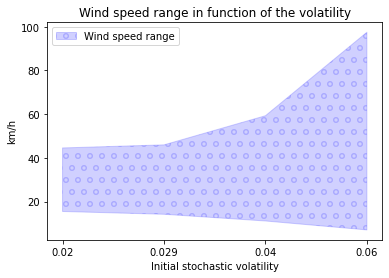
Figure 14: Wind speed range as function of the uncertainty parameter.

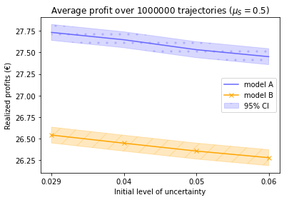
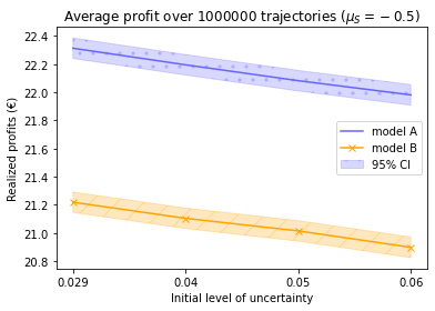
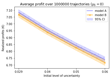
Figure 15: Realized profits for different values of the price trend

The simulated average profit for the two producers is shown in Figure 15. We see that in both models, the average profit decreases as function of the forecast uncertainty level. The presence of a price trend leads both for higher profits for the two models and a clear improvement of performance of model A compared to model B. In the case where the price is a martingale the result is not obvious since the confidence intervals of the average profits overlap to a large extent: this result needs to be further investigated. The observations made from Figure 15 are confirmed in Table 8 where we show the relative profits computed as follows:

$$\frac{\text{Profit(Model A)}-\text{Profit(Model B)}}{\text{Profits(Model B)}}\times 100.$$

$\mu_{S}$ (€/MWh.h)	Relative profits
	in $\%$
$0$	$+0.27$
$0.5$	$\mathbf{+4.49}$
$-0.5$	$\mathbf{+5.15}$

Table 8: Relative profits of Model A (taking into account stochastic forecast uncertainty) compared to Model B. Bold values are statistically significant at 95% level.

In the literature, estimations of the trend in the intraday electricity market price are scarce. A recent empirical study by Glas et Al. [15] reports the presence of a small trend composed of a constant part (0.0433 €/MWh²) and a permanent price impact (0.0017 €/MWh²). Hence taking into account the evolution of the forecast uncertainty as it is done in the model we propose seem to be adapted to the market reality and impacts the strategies in a way that increases significantly the profits.

Appendix

4.3 Talagrand diagrams and PIT histograms for lead times 36h and 48h

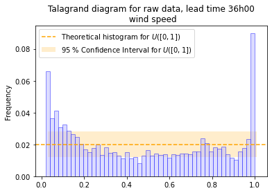
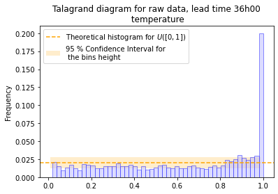
Figure 16: Talagrand diagrams for the wind speed and the temperature, lead time $36h00$

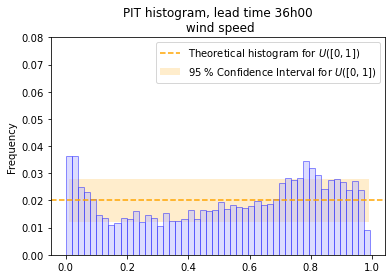
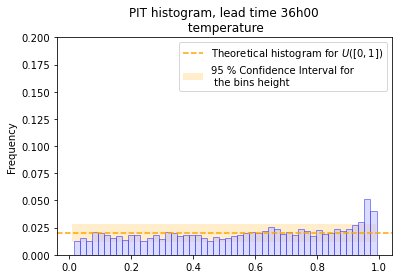
Figure 17: PIT histogram for the wind speed and the temperature, lead time $36h00$

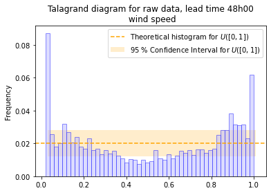
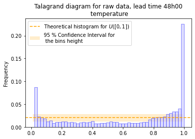
Figure 18: Talagrand diagrams for the wind speed and the temperature, lead time $48h00$

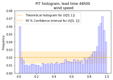
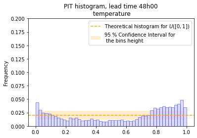
Figure 19: PIT histogram for the wind speed and the temperature, lead time $48h00$

References

- [1] K. Aas and I. H. Haff, The generalized hyperbolic skew student’st-distribution, Journal of financial econometrics, 4 (2006), pp. 275–309.
- [2] R. Aïd, P. Gruet, and H. Pham, An optimal trading problem in intraday electricity markets, Mathematics and Financial Economics, 10 (2016), pp. 49–85.
- [3] J. Badosa, E. Gobet, M. Grangereau, and D. Kim, Day-ahead probabilistic forecast of solar irradiance: a stochastic differential equation approach, in Forecasting and Risk Management for Renewable Energy, Springer, 2017, pp. 73–93.
- [4] S. Baran, Probabilistic wind speed forecasting using bayesian model averaging with truncated normal components, Computational Statistics & Data Analysis, 75 (2014), pp. 227–238.
- [5] S. Baran and S. Lerch, Log-normal distribution based ensemble model output statistics models for probabilistic wind-speed forecasting, Quarterly Journal of the Royal Meteorological Society, 141 (2015), pp. 2289–2299.
- [6] , Mixture emos model for calibrating ensemble forecasts of wind speed, Environmetrics, 27 (2016), pp. 116–130.
- [7] O. E. Barndorff-Nielsen, Processes of normal inverse gaussian type, Finance and stochastics, 2 (1997), pp. 41–68.
- [8] D. Belomestny, A. Kolodko, and J. Schoenmakers, Regression methods for stochastic control problems and their convergence analysis, SIAM Journal on Control and Optimization, 48 (2010), pp. 3562–3588.
- [9] A. Bensoussan and A. Brouste, Cox–ingersoll–ross model for wind speed modeling and forecasting, Wind Energy, 19 (2016), pp. 1355–1365.
- [10] B. Bouchard and X. Warin, Monte-carlo valuation of american options: facts and new algorithms to improve existing methods, in Numerical methods in finance, Springer, 2012, pp. 215–255.
- [11] J. Collet, O. Féron, and P. Tankov, Optimal management of a wind power plant with storage capacity, in Forecasting and Risk Management for Renewable Energy, Springer, 2017, pp. 229–246.
- [12] D. Dufresne, The distribution of a perpetuity, with applications to risk theory and pension funding, Scandinavian Actuarial Journal, 1990 (1990), pp. 39–79.
- [13] O. Féron, P. Tankov, and L. Tinsi, Price formation and optimal trading in intraday electricity markets, arXiv preprint arXiv:2009.04786, (2020).
- [14] H. Gevret, N. Langren’e, J. Lelong, X. Warin, and A. Maheshwari, Stochastic optimization library in c++, hal-01361291v1, (2018).
- [15] S. Glas, R. Kiesel, S. Kolkmann, M. Kremer, N. G. von Luckner, L. Ostmeier, K. Urban, and C. Weber, Intraday renewable electricity trading: Advanced modeling and numerical optimal control, Journal of Mathematics in Industry, 10 (2020), p. 3.
- [16] T. Gneiting, F. Balabdaoui, and A. E. Raftery, Probabilistic forecasts, calibration and sharpness, Journal of the Royal Statistical Society: Series B (Statistical Methodology), 69 (2007), pp. 243–268.
- [17] T. Gneiting, A. E. Raftery, A. H. Westveld III, and T. Goldman, Calibrated probabilistic forecasting using ensemble model output statistics and minimum crps estimation, Monthly Weather Review, 133 (2005), pp. 1098–1118.
- [18] E. B. Iversen, J. M. Morales, J. K. Møller, and H. Madsen, Short-term probabilistic forecasting of wind speed using stochastic differential equations, International Journal of Forecasting, 32 (2016), pp. 981–990.
- [19] M. Jeanblanc, M. Yor, and M. Chesney, Mathematical methods for financial markets, Springer Science & Business Media, 2009.
- [20] R. Kiesel and F. Paraschiv, Econometric analysis of 15-minute intraday electricity prices, Energy Economics, 64 (2017), pp. 77–90.
- [21] S. Lerch and T. L. Thorarinsdottir, Comparison of non-homogeneous regression models for probabilistic wind speed forecasting, Tellus A: Dynamic Meteorology and Oceanography, 65 (2013), p. 21206.
- [22] F. A. Longstaff and E. S. Schwartz, Valuing american options by simulation: a simple least-squares approach, The review of financial studies, 14 (2001), pp. 113–147.
- [23] P. Pinson, C. Chevallier, and G. N. Kariniotakis, Trading wind generation from short-term probabilistic forecasts of wind power, IEEE Transactions on Power Systems, 22 (2007), pp. 1148–1156.
- [24] P. Pinson et al., Wind energy: Forecasting challenges for its operational management, Statistical Science, 28 (2013), pp. 564–585.
- [25] A. E. Raftery, T. Gneiting, F. Balabdaoui, and M. Polakowski, Using bayesian model averaging to calibrate forecast ensembles, Monthly weather review, 133 (2005), pp. 1155–1174.
- [26] A. Skajaa, K. Edlund, and J. M. Morales, Intraday trading of wind energy, IEEE Transactions on power systems, 30 (2015), pp. 3181–3189.
- [27] Z. Tan and P. Tankov, Optimal trading policies for wind energy producer, SIAM Journal on Financial Mathematics, 9 (2018), pp. 315–346.
- [28] T. L. Thorarinsdottir and T. Gneiting, Probabilistic forecasts of wind speed: Ensemble model output statistics by using heteroscedastic censored regression, Journal of the Royal Statistical Society: Series A (Statistics in Society), 173 (2010), pp. 371–388.
- [29] J. N. Tsitsiklis and B. Van Roy, Optimal stopping of markov processes: Hilbert space theory, approximation algorithms, and an application to pricing high-dimensional financial derivatives, IEEE Transactions on Automatic Control, 44 (1999), pp. 1840–1851.
- [30] D. S. Wilks, Smoothing forecast ensembles with fitted probability distributions, Quarterly Journal of the Royal Meteorological Society: A journal of the atmospheric sciences, applied meteorology and physical oceanography, 128 (2002), pp. 2821–2836.
- [31] M. Zugno, T. Jónsson, and P. Pinson, Trading wind energy on the basis of probabilistic forecasts both of wind generation and of market quantities, Wind Energy, 16 (2013), pp. 909–926.