Exploring Context Generalizability in Citywide Crowd Mobility Prediction: An Analytic Framework and Benchmark

Abstract

Contextual features are important data sources for building citywide crowd mobility prediction models. However, the difficulty of applying context lies in the unknown generalizability of contextual features (e.g., weather, holiday, and points of interests) and context modeling techniques across different scenarios. In this paper, we present a unified analytic framework and a large-scale benchmark for evaluating context generalizability. The benchmark includes crowd mobility data, contextual data, and advanced prediction models. We conduct comprehensive experiments in several crowd mobility prediction tasks such as bike flow, metro passenger flow, and electric vehicle charging demand. Our results reveal several important observations: (1) Using more contextual features may not always result in better prediction with existing context modeling techniques; in particular, the combination of holiday and temporal position can provide more generalizable beneficial information than other contextual feature combinations. (2) In context modeling techniques, using a gated unit to incorporate raw contextual features into the deep prediction model has good generalizability. Besides, we offer several suggestions about incorporating contextual factors for building crowd mobility prediction applications. From our findings, we call for future research efforts devoted to developing new context modeling solutions.

1 Introduction

Understanding and modeling citywide crowd mobility is of significant importance for the advancement of smart city applications, encompassing critical fields such as safety and security [1, 2], crowd sensing [3], personalized service recommendation [4, 5], resource allocation and energy saving [6, 7, 8, 9, 10, 11], transportation planning [12] and urban infrastructure development [13]. Accurate prediction of citywide crowd mobility is a fundamental and essential research challenge, representing a crucial abstraction of numerous tasks including bike-sharing flow forecasting [14, 15, 16, 17], ride-sharing demand predicting [18, 19, 20, 21, 22, 23], and traffic speed prediction [24, 25]. These predictive capabilities facilitate the optimization and effective implementation of various urban services, enabling informed decision-making and resource allocation in a rapidly evolving city environment.

Contextual factors (e.g., weather, holidays) have proven beneficial for citywide crowd mobility prediction [26, 27]. Taking weather context as an example, rising temperatures will promote the usage of bike-sharing [14], and heavy rains will lessen the usage of both bike-sharing and online ride-hailing [28]. In general, context is any information that can be used to characterize the situation of an entity, where an entity can be a person, place, or physical/computational object [29]. Comprehending and modeling contextual factors assumes critical significance in crowd mobility prediction tasks, as it has the potential to furnish valuable supplementary insights into the acquisition of specific spatiotemporal patterns. By incorporating context awareness into predictive models, an enriched understanding of crowd dynamics can be achieved, leading to more accurate and robust mobility forecasts [30, 26, 31].

To achieve accurate crowd mobility prediction, researchers have recognized the importance of considering spatial and temporal correlations and have proposed various techniques to model spatiotemporal dependencies, including attention mechanisms [32, 33, 34] and graph convolution networks [24, 35, 16]. This problem is commonly referred to as spatiotemporal crowd flow prediction (STCFP) [26, 36, 37] or spatiotemporal traffic prediction (STTP) problem [38, 39]. Temporal correlations elucidate the connection between future and past flows, whereas spatial correlations primarily capture the interrelationship between different geographical locations. Furthermore, extensive studies have been conducted to explore the generalizability of spatiotemporal correlations [39]. By comprehending and leveraging these spatiotemporal correlations, the predictive capabilities of spatiotemporal models can be enhanced, leading to more robust and reliable predictions of crowd mobility.

However, despite the utilization of specific contextual features in certain applications [14], the generalizability of contextual features is still under-investigated. For example, POIs (Points-Of-Interests) data is effective in taxi demand prediction problems [18], but whether POIs data is still beneficial in other scenarios remains to be evaluated. Besides, while pioneering studies propose various context modeling techniques such as Adding [40], Embedding [16], and Gating [41], it is still hard to select appropriate context modeling techniques for a given problem since the generalizability of these modeling techniques is unknown.

Overall, analyzing the generalizability of contextual features and context modeling techniques is of significant value for building effective mobility prediction models. Meanwhile, this analysis is challenging in the following aspects:

Unknown generalizability of contextual features. Most studies directly consider a specific set of contextual features without carefully analyzing whether the selection of these features is optimal. To the best of our knowledge, no previous study has thoroughly compared the generalizability of contextual features across different application scenarios.

Lacking a taxonomy of context modeling techniques. Previous studies propose various context modeling techniques. For the convenience of analyzing the generalizability of context modeling techniques, a comprehensive taxonomy is desired.

Unknown generalizability of context modeling techniques. Though several context modeling techniques have been proposed, it is hard to determine a suitable modeling technique given an STCFP task. As far as we know, no previous study has analyzed the generalizability of different context modeling techniques across scenarios.

To sum up, in this paper, we aim to analyze the generalizability of both contextual features and context modeling techniques in STCFP applications. We conduct a large-scale analytical and experimental empirical study. Particularly, we try to give some design guidelines for the research community and make the following contributions:

• To the best of our knowledge, this is the first study that focuses on investigating how contextual factors (both features and modeling techniques) would generally and quantitatively impact crowd mobility prediction performance in various practical scenarios. By answering this critical but under-investigated problem, we expect that this research can inspire researchers and practitioners to learn how to efficiently incorporate contextual factors in crowd mobility prediction models and applications.

• By surveying recent studies, we categorize the mostly-used contextual features in literature, including weather, holiday, temporal position, and POIs. Additionally, a new unified analytic framework for context modeling techniques in STCFP models is developed, summarizing a total of 14 techniques. While ten techniques are leveraged in literature, the other four are newly established and investigated by our work.

• We have created and released an experimental repository that provides crowd mobility data, aligned contextual data, and state-of-the-art STCFP models. The repository covers three applications: bike-sharing usage, metro passenger flow, and electronic vehicle demand. Researchers can utilize this platform to experiment with their own STCFP applications and explore the effectiveness and generalizability of the context.

• Our extensive experiments reveal a surprising and counter-intuitive finding — with current context modeling techniques, introducing more contextual features (e.g., weather) would often degrade the prediction performance. However, we find that holiday and temporal position features generally provide beneficial information, while weather and POIs do not offer significant improvements and may even have negative impacts. Based on these observations, we provide suggestions for crowd mobility prediction models to incorporate contextual factors. Furthermore, we emphasize the need for future research to develop new context processing and modeling solutions that fully exploit the potential of contextual features.

2 Problem and Generalizability

2.1 Problem Formulation

Definition 1 (Location). The set of $N$ locations where the crowd flow are observed is denoted as $\mathcal{L}=\{l_{1},l_{2},...,l_{N}\}$. The locations can both represent the equal-sized grid in dock-less applications (e.g., ride-sharing [18, 19, 20, 21, 22, 23]) or the dock stations in dock-based applications (e.g., metro passenger flow [42]).

Definition 2 (Crowd flow time series). Given a set of $N$ locations $\mathcal{L}$, $\textbf{X}_{t}\in\mathbb{R}^{N\times D}$ is the crowd flow observations of $N$ locations during the time interval $t$. $D$ is the feature dimension of a location. The crowd flow time series from time interval 1 to the time interval $t$ is $\mathcal{X}_{1:t}=\{\textbf{X}_{1},....,\textbf{X}_{t}\}$

Definition 3 (Temporal contextual features). Temporal contextual features are characterized by their variabilities within short time periods, such as one hour or one day. One example of such features is the weather, which can change abruptly from sunny to rainy within a short time interval. In urban applications, these features tend to be consistent across different locations at the same moment. For brevity, we will refer to these features as temporal contextual features, which are primarily sensitive to changes in the temporal dimension. The temporal contextual features from time interval 1 to the time interval $T$ can be represented as $\mathcal{T}_{1:T}\in\mathbb{R}^{T\times E_{t}}$, where $E_{t}$ denotes the feature dimension of the temporal context.

Definition 4 (Spatial contextual features). Spatial contextual features exhibit variability in their locations, with Points of Interest (POIs) being one example. POIs in business areas are typically more numerous than those in industrial parks. These features are known to remain relatively stable over long periods (POIs records from OpenStreetMap only change a few samples in one day). Notably, spatial contextual features are primarily sensitive to changes in the spatial dimension. In this regard, we represent the spatial contextual features of $N$ locations using $\mathcal{S}\in\mathbb{R}^{N\times E_{s}}$, where $E_{s}$ refers to the feature dimension of the spatial context.

Problem 1. First, we formulate the context-engaged Spatio-Temporal Crowd Flow Prediction problem. Suppose that we have a set of $N$ locations $\mathcal{L}$. Given $\mathcal{X}_{(t-P):t}$, the past $P$ step historical crowd flows observation, we aim to learn a function $f$ which maps $\mathcal{X}_{(t-P):t}$ and the corresponding temporal contextual features $\mathcal{T}_{(t-P):t}\in\mathbb{R}^{P\times E_{t}}$ and spatial contextual features $\mathcal{S}\in\mathbb{R}^{N\times E_{s}}$ to the observation in the next time slots $t+1$:

$$[\mathcal{X}_{(t-P):t},\mathcal{T}_{(t-P):t},\mathcal{S}]\xrightarrow{f}\hat{\textbf{X}}_{t+1}$$ (1)

Many real-world applications can be formulated as the above problem, such as bike-sharing [14, 15, 16, 17], ride-sharing [18, 19, 20, 21, 22, 23], metro passenger flow [42, 43, 44] and so on.

2.2 Generalizability

In this paper, we mainly focus on two context generalizability issues rather than specific applications: Feature Generalizability and Technique Generalizability:

Feature Generalizability. As existing STCFP applications may involve different kinds of contextual features (e.g., weather and holiday for bike-sharing applications[16], weather and POIs for ride-sharing applications [23]. More details are in Table I), the feature generalizability refers to: Given several kinds of contextual features, which feature combination is generalizable to be effective for various applications?

Technique Generalizability: Previous researchers have proposed many context modeling techniques (e.g., gating mechanism [41, 45] and Concatenate [21, 16, 42, 46, 32, 47]) and many spatiotemporal dependencies modeling techniques (e.g., STGCN [35], GraphWaveNet [48], and AGCRN[49]) for a variety of applications. The technique generalizability refers to: (1) Given a certain kind of context modeling technique, is it generalizable to be effective for various applications? (2) Regarding different spatiotemporal modeling techniques, is a context modeling technique generalizable to be effective for various spatiotemporal models?

3 Analytical Studies on Contextual Features

In this section, we analyze contextual features mentioned in recent studies and introduce contextual data preprocessing methods. We provide examples of temporal and spatial contextual features in Figure 1 for better understanding.

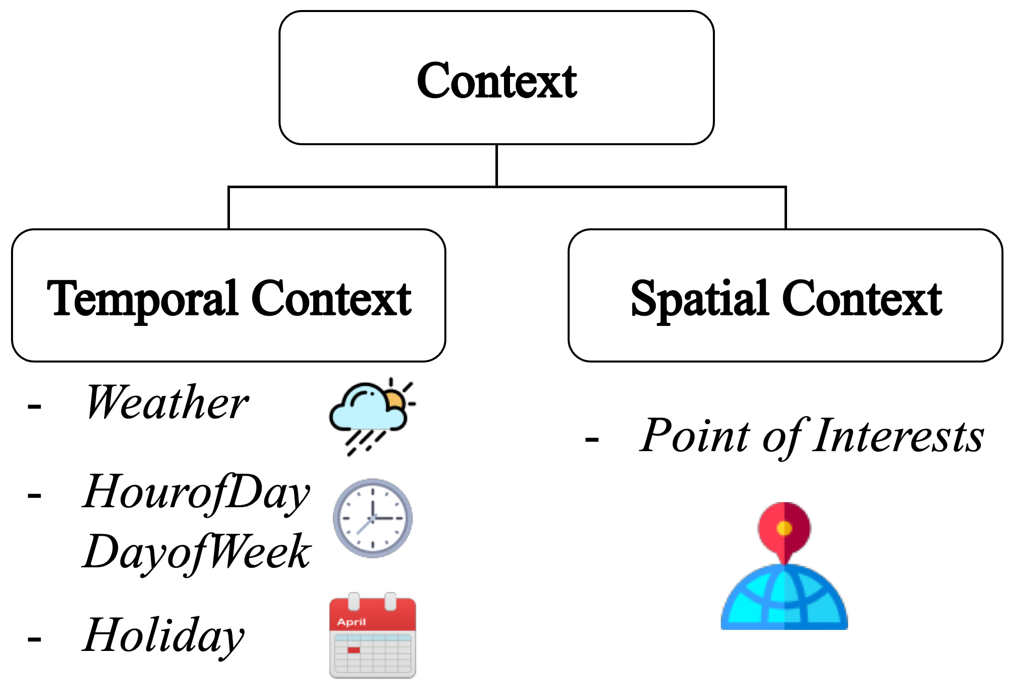
Figure 1: Examples of temporal and spatial contextual features.

TABLE I: Contextual features and context modeling techniques in STCFP studies. ‘TC’ and ‘SC’ are temporal and spatial contextual features, respectively. (T: Temperature; H: Humidity; V: Visibility; WS: Wind Speed; WD: Wind Degree; AQ: Air Quality; S: Weather State)

Model	Weather	Holiday	Temporal Position	POIs	Modeling Technique
	(SC)	(TC)	(TC)	(SC)
Bike-sharing
Li et al. [14]	T;WS;S				Feature Concatenate
Yang et al. [15]	T;H;V;WS;S		✓		Feature Concatenate
Chai et al. [16]	T;WS;S	✓			Emb-Concat
Li et al. [17]	T;WS;S	✓	✓		Feature Concatenate
Ridesharing
Tong et al. [18]	T;H;WS;WD;AQ;S	✓	✓	✓	Feature Concatenate
Ke et al. [19]	T;H;V;WS;S		✓		LSTM-Add
Wang et al. [20]	T;AQ;S				MultiEmb-Concat
Zhu et al. [21]		✓			Raw-Concat
Yao et al. [22]	T;S	✓			EarlyConcat
Saadallah et al. [23]	T;WS;S			✓	Feature Concatenate
Metro Passenger Flow
Liu et al. [42]	S		✓		MultiEmb-Concat
Traffic Flow
Yi et al. [25]			✓		Emb-Add
Zhang et al. [50]			✓		EarlyConcat
Barnes et al. [51]			✓		Feature Concatenate
Zheng et al. [52]	T;WS;V;S	✓	✓	✓	Feature engineering + CNN
Chen et al. [53]	S	✓	✓		Emb-Concat
Zhang et al. [47]	WS;T;S	✓	✓		MultiEmb-Concat
Yuan et al. [46]	S	✓	✓		Emb-Concat
Citywide Crowd Flow
Hoang et al. [28]	T				Feature Concatenate
Zhang et al. [40]			✓		Raw-Add
Zhang et al. [26]	T;WS;S	✓			Emb-Add
Zonoozi et al. [54]			✓		Raw-Add
Lin et al. [31]			✓	✓	EarlyConcat
Zhang et al. [41]	T;WS;S	✓			Raw-Gating
Chen et al. [55]	S		✓		EarlyConcat
Sun et al. [45]	T;WS;S	✓	✓		Emb-Gating/Add
Jiang et al. [56]			✓		EarlyConcat
Liang et al. [57]	T;WS;S	✓		✓	EarlyConcat

3.1 Contextual Features

We here elaborate on four kinds of contextual features including three temporal contextual features (i.e., weather, holiday, and temporal position) and one spatial contextual feature (i.e., POIs).

Weather. In general, weather features such as temperature, humidity, wind speed, and weather states (e.g., cloudy and thunderstorms) are associated with short-term fluctuations in the atmosphere, which can impact crowd flow dynamics [14, 28, 58]. For example, a rise in temperature may result in increased use of bike-sharing services [14], while heavy rains and strong winds may decrease the utilization of bike-sharing and online ride-hailing services [28]. The impact of weather on crowd flow may vary depending on the specific application scenario of STCFP. Notably, temperature and weather states are the most commonly examined contextual features in existing literature, as indicated in the second column of Table I.

Holiday. During the holiday, people usually take a break from work or other regular activities in order to relax or travel. As a result, the crowd flow daily patterns are closely related to holidays. There is an obvious migration flow from urban residential areas to business areas during workdays, but this pattern is unclear on holidays [26]. Hoang et al. also reveal that the subway traffic pattern on weekends is obviously different from that on weekdays [28].

Temporal Position. The temporal dynamics of crowd flow exhibit significant variation across different days of the week, with higher flow volumes typically observed on Friday evenings compared to Thursday evenings. Furthermore, hourly flow patterns within a given day can also differ, with peak flow volumes during morning and evening rush hours far exceeding those during off-peak periods. The above phenomena reveal the temporal heterogeneity of crowd flow [59]. To capture these temporal variations in crowd flow, two discrete indicators are introduced to encode temporal position information [42, 25]:

• HourofDay indicates where the current time is in one day (what time it is), and its value ranges from 0 to 23 (representing 0 o’clock to 23 o’clock).

• DayofWeek indicates where the current time is in one week (which day it is). The value range of DayofWeek is between Monday and Sunday.

Notably, temporal position features can easily adapt to temporal fine-grained STCFP tasks (e.g., 15-minute prediction) by encoding every time interval to a distinct value within a day.

Points Of Interests. POIs refer to specific locations or landmarks that are significant or interesting to people such as residential areas, business areas, and tourist attractions. These can be natural or man-made attractions, historical sites, cultural centers, entertainment venues, or any other location that draws the attention of people. POIs are often marked on maps or included in travel guides and navigation systems to help people navigate and find their way around unfamiliar areas. They can also be used to plan trips or activities, as well as to promote tourism and local economies. POIs greatly improve our understanding of these locations’ traffic patterns [60], which are usually considered beneficial information to model spatial correlations [18, 32, 61].

3.2 Contextual Features Preprocessing Methods

To enhance the exploitation of contextual features, we elaborate on several typical feature prepossessing techniques for weather, holiday, temporal position, and POIs. Our study also includes a detailed discussion on context modeling techniques, which are introduced in Section 4. It is worth noting that these modeling techniques usually employ learning paradigms that involve learnable parameters and thus differ from the contextual prepossessing methods.

Weather. The weather context encompasses both numerical and categorical features, which necessitates consideration in machine learning approaches such as neural networks. Numerical features, such as temperature (^∘F), humidity (%), and wind speed (m/s), hold specific numerical values and can be readily utilized. In contrast, categorical contextual features, such as weather states (e.g., sunny, rainy, etc.), require transformation into numerical features. One-hot encoding and hand-crafted encoding that categorizes weather states into good (e.g., sunny, cloudy) and bad weather (e.g., rainy, stormy, dusty) both can be used for this purpose [28, 55].

Holiday and Temporal Position. For the holiday context, we can use a binary variable to indicate whether a day is a holiday. Moreover, we also may include other features such as the type of holiday (e.g. Christmas, Thanksgiving). In a similar manner, the temporal position context, including HourofDay and DayofWeek, can also be transformed to enhance analysis. For instance, the HourofDay can be represented as a one-hot vector with a length of 24, indicating the position of a given hour in a day. Similarly, the DayofWeek can be encoded as a seven-dimensional vector. These transformations have been utilized in prior research [25, 42].

POIs. For POIs, researchers often count the POIs density of different categories as features [18]. Due to the disturbances caused by various region functions, previous research proposes an elaborated feature engineering method to encode POIs features (i.e., the Inherent Influence Factor) [52]. To differentiate the importance of each type of POIs to each region, previous research applies the Term Frequency–Inverse Document Frequency (TF-IDF) to encode POIs features, where the POIs are considered as words and the regions are the documents [62, 61].

Note that, in the above discussions, one-hot encoding has been widely used for transforming categorical features into numerical features, it can result in an explosion of feature dimensions, thereby increasing the risk of the curse of dimensionality. To address this issue, some researchers have manually reduced feature dimensions by categorizing weather states into good and bad weather categories. Others use Embedding [16, 26] to achieve dimension reduction, which will be introduced in the next section.

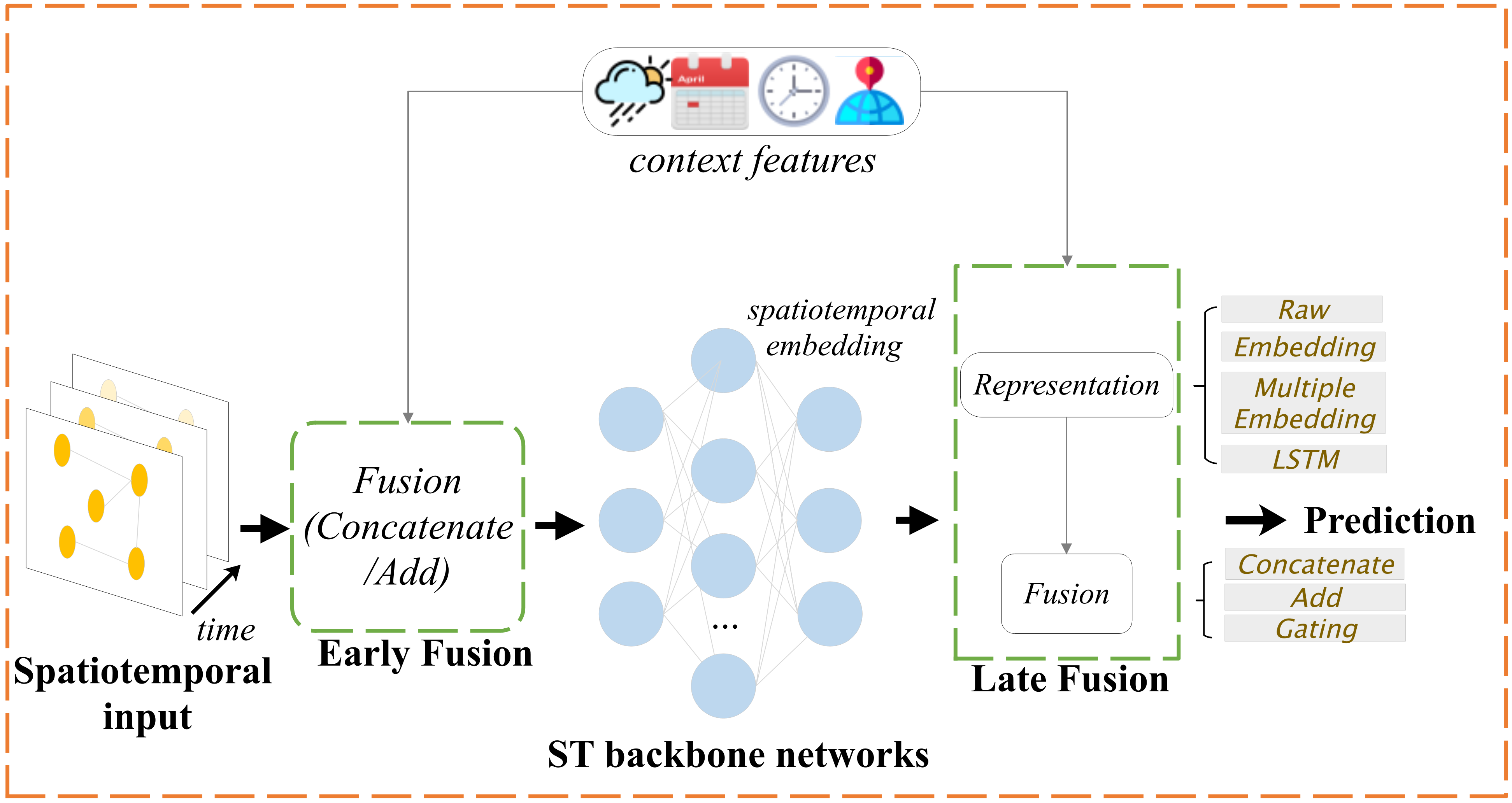
Figure 2: The proposed context modeling analytic framework. Existing modeling techniques can be categorized as Early Joint Modeling and Late Fusion. The backbone networks can be STMGCN, STMeta, or other spatiotemporal networks.

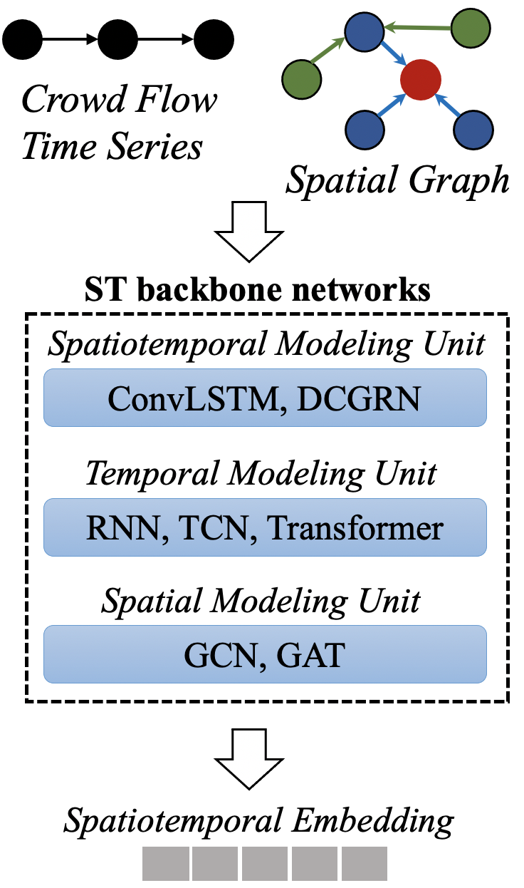
Figure 3: ST backbone networks consist of spatiotemporal modeling units or stacking of several temporal modeling units and spatial modeling units.

4 Analytical Studies on Context Modeling Techniques

4.1 Analytic Framework

To illustrate the context modeling techniques more clearly, we first introduce a flexible and general context modeling analytic framework (Figure 3). It contains two vital components, namely the ST backbone networks and the context modeling techniques.

The ST backbone networks (Figure 3) take spatiotemporal input (e.g., crowd flow time series and spatial graphs) and learn diverse spatiotemporal embeddings, having been well-studied in the previous research [26, 63, 64, 49, 46, 65, 39]. Typically, ST backbone networks can be simplified to a function $g$ :

$$g:\mathcal{X}_{(t-P):t}\in\mathbb{R}^{P\times N\times D}\rightarrow\mathcal{X}^{emb}_{t}\in\mathbb{R}^{N\times D_{1}}$$ (2)

where $D_{1}$ is the number of features of spatiotemporal embedding. ST backbone networks extract spatiotemporal embedding by stacking several temporal modeling units (e.g., LSTM [66], TCN [67], and Transformer [68]) and spatial modeling units (e.g., GCN [69, 16] and GAT [70, 34]). Previous research also has proposed several spatiotemporal modeling units that can simultaneously model spatiotemporal dependencies (e.g., ConvLSTM [71] and DCGRU [24]).

Our analytic framework classifies existing context modeling techniques into Early Joint Modeling and Late Fusion. Early joint modeling fuses contextual features with spatiotemporal input before capturing spatiotemporal dependencies, while late fusion fuses contextual features with spatiotemporal embedding learned by ST backbone networks. The main difference is Early Joint Modeling uses the same spatiotemporal backbone networks to extract both spatiotemporal embedding and context embedding while Late Fusion uses distinct modules to learn context embedding.

Note that our context modeling analytic framework is developed mainly for deep learning models (we summarize the context modeling techniques in Table I). Traditional statistical learning models such as XGBoost [72] usually directly fuse contextual features by concatenating [14, 15, 18, 17].

4.2 Early Joint Modeling

Early joint modeling refers to fusing contextual features with raw spatiotemporal inputs before capturing spatiotemporal dependencies via ST backbone networks. Hence, in addition to getting spatiotemporal embedding of spatiotemporal inputs, the ST backbone networks will also extract the spatiotemporal dependencies of contextual features synchronously. For example, researchers combine the features of DayofWeek, HourofDay and POIs’ population distribution map by using adding and then applying the ResPlus structure to capture spatial dependencies between distant locations [31, 73]. Yao et al. first concatenate spatial features and contextual features (including weather and holiday) and then capture temporal patterns by LSTM [22, 74].

Notably, weather, holiday and temporal position are temporal contextual features (i.e., $\mathcal{T}_{(t-P):t}\in\mathbb{R}^{P\times E_{t}}$) and POIs are spatial contextual features (i.e., $\mathcal{S}\in\mathbb{R}^{N\times E_{s}}$). To align their feature dimension with crowd flow time series (i.e., $\mathcal{X}_{(t-P):t}\in\mathbb{R}^{P\times N\times D}$), replicate technique (details in Figure 5) is widely used [19, 41, 36]. After replicating, the duplicated temporal and spatial contextual features are $\mathcal{T}^{\prime}_{(t-P):t}\in\mathbb{R}^{P\times N\times E_{t}}$ and $\mathcal{S}^{\prime}\in\mathbb{R}^{P\times N\times E_{s}}$, respectively. As the semantic meaning of features dimension (i.e., the last axis) is the same, for brevity, we merge them into the spatiotemporal contextual features $\mathcal{E}_{(t-p):t}\in\mathbb{R}^{P\times N\times(E_{t}+E_{s})}$ by concatenating.

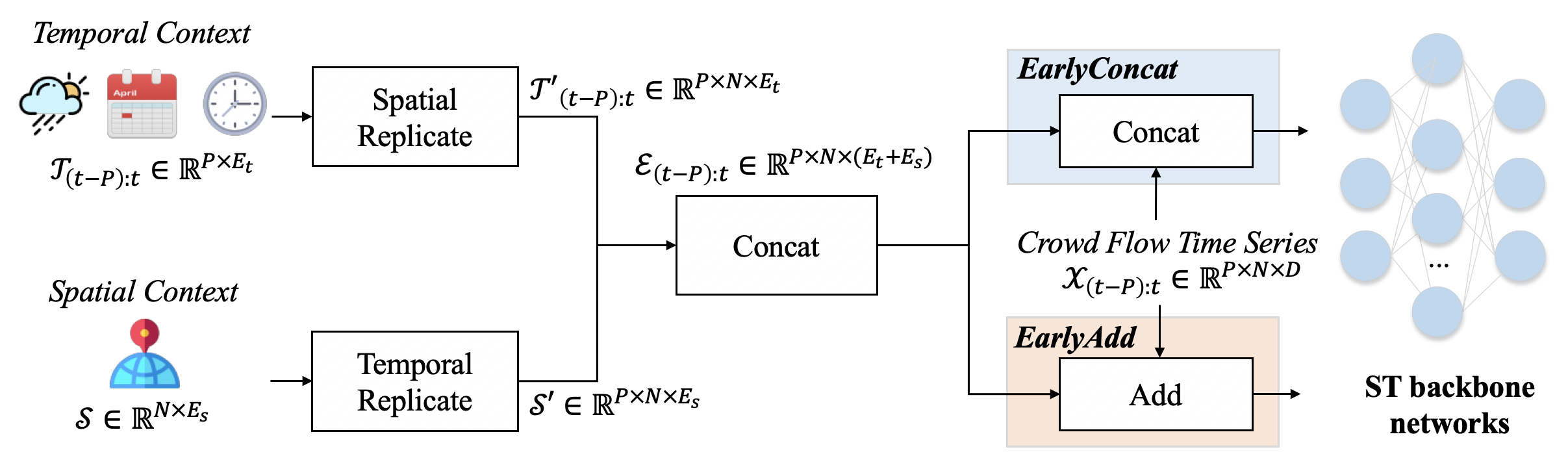
Figure 4: Details of Early Joint Modeling.

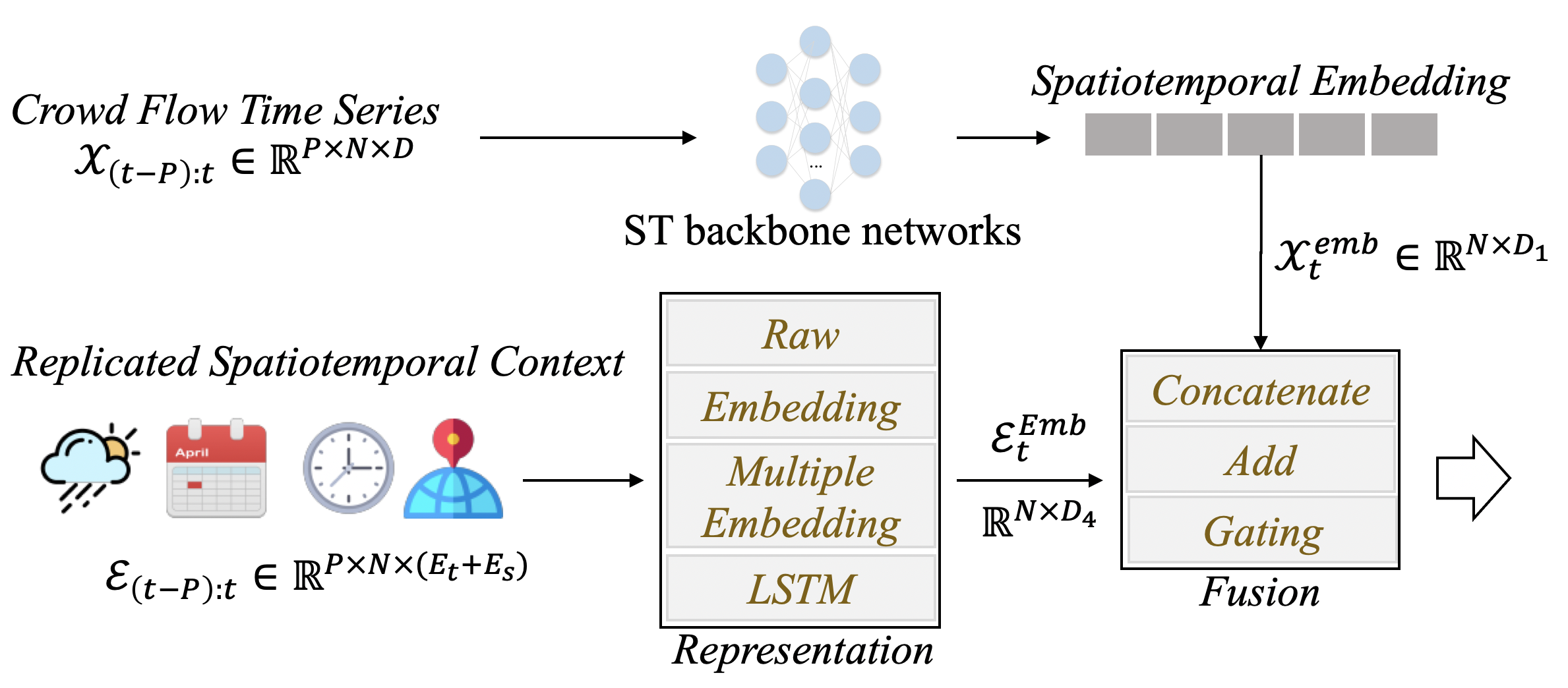
Figure 5: Details of Late Fusion.

As shown in Figure 5, both Concatenate and Add can fuse spatiotemporal contextual features $\mathcal{E}_{(t-P):t}$ and crowd flow time series features $\mathcal{X}_{(t-P):t}$, and we name these two modeling techniques EarlyAdd and EarlyConcat, respectively. Recall that $P$ is the number of historical observations, $N$ is the number of locations, $E_{s}+E_{t}$ and $D$ are the dimensions of contextual features and spatiotemporal inputs. We denote the output of early joint modeling as $\mathcal{O}^{Early}$ and the formula of EarlyConcat is:

$$\mathcal{O}^{Early}_{(t-P):t}=Concat(\mathcal{E}_{(t-P):t};\mathcal{X}_{(t-P):t})\in\mathbb{R}^{P\times N\times(D+E_{s}+E_{t})}$$ (3)

Similarly, the output of early joint modeling given by EarlyAdd is:

$$\mathcal{O}^{Early}_{(t-P):t}=\mathcal{E}_{(t-P):t}\times W_{e}+\mathcal{X}_{(t-P):t}\times W_{st}+b_{e}\in\mathbb{R}^{P\times N\times D2}$$ (4)

where $W_{e}\in\mathbb{R}^{(E_{s}+E_{t})\times D_{2}}$, $W_{st}\in\mathbb{R}^{D\times D_{2}}$ and $b_{e}\in\mathbb{R}^{D_{2}}$ are trainable parameters. $D,D_{2}$ are the dimension of the crowd flow time series and the fused features obtained by EarlyAdd, respectively.

Then the ST backbone networks can jointly model spatiotemporal dependencies of both crowd flow series and contextual features. Equation 2 can be rewrite as:

$$g^{\prime}:\mathcal{O}^{Early}_{(t-P):t}\in\mathbb{R}^{P\times N\times D^{\prime}}\rightarrow\mathcal{X}^{emb}_{t}\in\mathbb{R}^{N\times D_{3}}$$ (5)

where $D_{3}$ is the dimension of joint embedding of crowd flow series and contextual features. The joint embedding usually is fed to the output layer and gives predictions. $D^{\prime}$ is $D$+$E_{s}$+$E_{t}$ or $D_{2}$ when applied EarlyConcat and EarlyAdd, respectively.

4.3 Late Fusion

Late fusion combines contextual features and spatiotemporal embedding learned by ST backbone networks, which is adept at fusing data from different domains [40]. In this study, we investigate existing late fusion methods and identified two stages in the process. The first stage involves the learning of diverse contextual embedding, while the second stage entails fusing the context embedding with spatiotemporal embedding for predictions. This two-stage approach is a common thread among the late fusion methods. These findings contribute to the understanding of the late fusion technique and provide insights for its future development and applications in the STCFP problem. We next elaborate on these two stages.

4.3.1 Context Representation Stage

The representation stage takes in $\mathcal{E}_{(t-p):t}$, the replicated spatiotemporal contextual features , and outputs the learned context embedding $\mathcal{E}^{Emb}_{t}\in\mathbb{R}^{N\times D_{4}}$. The following four techniques can be applied to conduct transformation as shown in Figure 5.

Raw. No transformations are applied to the spatiotemporal contextual features. Since the contextual features that are closer in time to the prediction moment should be more important, Raw keeps the contextual features closest to the prediction moment, namely $\mathcal{E}_{t-1}$.

Embedding. The embedding technique is widely used in various fields, such as NLP (Natural Language Processing). It maps sparse high-dimension features to dense low-dimension features. Many studies use fully-connected layers for embedding [16, 26]. For instance, Zhang et al. [26] use two fully-connected layers upon contextual features, and the first layer acts as an embedding layer. Embedding keeps the closest contextual features $\mathcal{E}_{t-1}$ and the embedding technique is applied to the feature dimension of $\mathcal{E}_{t-1}$ (i.e., the last axis).

Multiple Embedding. Different contextual features can be fed into multiple embedding layers [42, 32, 20]. For example, Liu et al. [42] use different embedding layers to model weather and temporal position, respectively. Multiple Embedding also uses the closest contextual features $\mathcal{E}_{t-1}$ and transforms the feature dimension of $\mathcal{E}_{t-1}$ (i.e., the last axis).

LSTM. Temporal contextual features (e.g., weather) usually are time-varying, and past contextual features may also impact future flow. For example, sudden heavy rain may immediately reduce the crowd flow, but when the rain stops, the crowd flow may be larger than ever. Ke et al. [19] use LSTM to capture temporal dependencies of weather. Unlike the above three representation techniques which focus on the closest contextual features $\mathcal{E}_{t-1}$, LSTM takes in the historical context series $\mathcal{E}_{(t-P):t}$.

4.3.2 Feature Fusion Stage

The fusion stage fuses the context embedding $\mathcal{E}^{emb}_{t}\in\mathbb{R}^{N\times D_{4}}$ with the spatiotemporal embedding $\mathcal{X}^{emb}_{t}\in\mathbb{R}^{N\times D_{1}}$ and outputs the fused embedding $\mathcal{O}_{t}^{Late}$ for prediction. The following three techniques are widely adopted in previous research (details are in Figure 6).

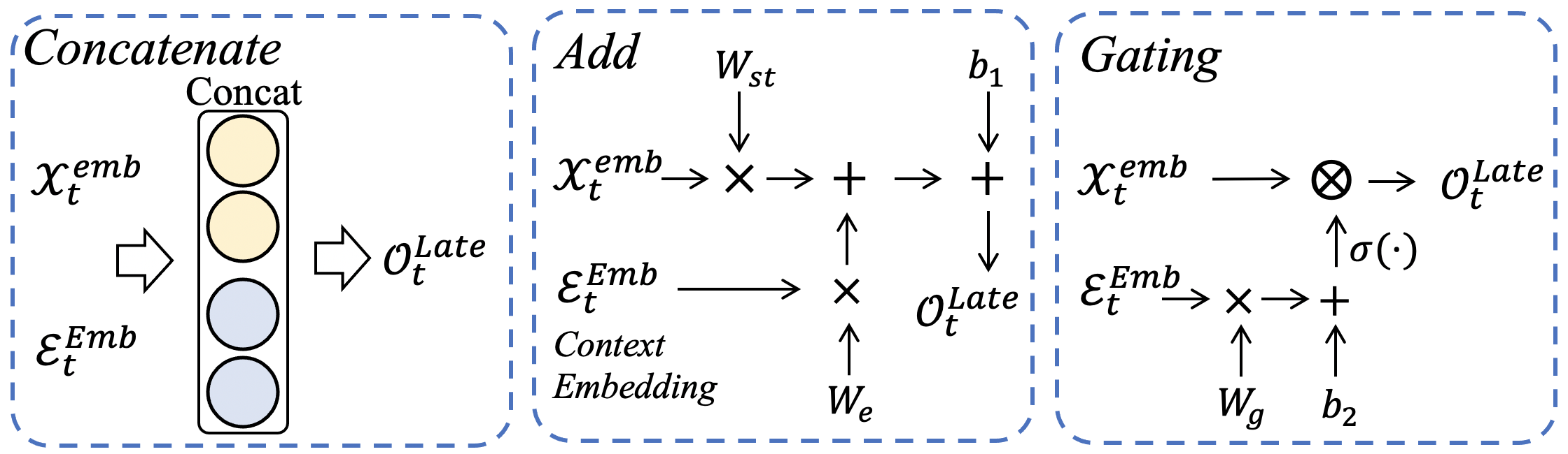
Figure 6: Details of Concatenate, Add and Gating.

Concatenate is a widely used technique that combines different features. Chai et al. [16] use a fully-connected layer as the embedding layer to represent features and then concatenate $\mathcal{E}^{emb}_{t}$ with spatiotemporal embedding $\mathcal{X}^{emb}_{t}$. The Concatenate formula is:

$$\mathcal{O}^{Late}_{t}=Concat(\mathcal{X}^{emb}_{t};\mathcal{E}^{emb}_{t})\in\mathbb{R}^{N\times(D_{1}+D_{4})}$$ (6)

Add first projects the context embedding $\mathcal{E}^{emb}_{t}$ and the spatiotemporal embedding $\mathcal{X}^{emb}_{t}$ into the feature space with the same dimension. Then it fuses them by adding the corresponding aligned features. The formula of Add is listed below. $W_{st}\in\mathbb{R}^{D_{1}\times D_{5}}$, $W_{e}\in\mathbb{R}^{D_{4}\times D_{5}}$, and $b_{1}\in\mathbb{R}^{D_{5}}$ are learnable parameters.

$$\mathcal{O}^{Late}_{t}=\mathcal{X}^{emb}_{t}\times W_{st}+\mathcal{E}^{emb}_{t}\times W_{e}+b_{1}$$ (7)

TABLE II: Late Fusion details consisting of representation and fusion stage. Modeling techniques with ‘*’ are newly found based on our analytic studies, which have never appeared in the literature to the best of our knowledge.

Name	Representation	Fusion	Literature
Raw-Concat	Raw	Concatenate	[21]
Raw-Add		Add	[40, 54]
Raw-Gating		Gating	[41]
Emb-Concat	Embedding	Concatenate	[16, 46]
Emb-Add		Add	[26, 25]
Emb-Gating		Gating	[45]
MultiEmb-Concat	Multiple Embedding	Concatenate	[42, 32, 20, 47]
MultiEmb-Add∗		Add	-
MultiEmb-Gating∗		Gating	-
LSTM-Concat∗	LSTM	Concatenate	-
LSTM-Add		Add	[19]
LSTM-Gating∗		Gating	-

Gating [41] regards the contextual features as the activation function of crowd flow. It first transforms the contextual embedding to the gating value $G$ and then uses $G$ to activate the spatiotemporal embedding:

$$G=\sigma(\mathcal{E}^{emb}_{t}\times W_{g}+b_{2})\in\mathbb{R}^{N\times D_{1}}$$ (8)

$$\mathcal{O}^{Late}_{t}=\sigma(G\otimes\mathcal{X}^{emb}_{t})$$ (9)

where ${W}_{g}\in\mathbb{R}^{D4\times D1}$ and $b_{2}\in\mathbb{R}^{D_{1}}$ are learnable parameters, ‘$\otimes$’ is the Hadamard product. $\sigma(\cdot)$ is the sigmoid function. The intuition of Gating is that features are like switches, and the crowd flows would be tremendously changed if a certain switch is activated.

In summary, by combining the above two stages, we list 12 (3*4) variants of Late Fusion Modelling techniques, as shown in Table II. It is worth noting that, with a comprehensive survey of the literature, we find that four variants never appeared in previous work. Meanwhile, we believe that these variants are reasonable context modeling techniques and we will also test them in our benchmark experiments.

5 Empirical Benchmark Setup

5.1 Datasets

We gather three crowd flow datasets comprising bike-sharing demand, metro passenger flow, and electric vehicle charging station usage, along with their corresponding contextual data such as weather, holiday, and POIs. The original crowd mobility records are processed at intervals of 30, 60, and 120 minutes. For detailed dataset descriptions, please refer to Appendix A.

5.2 Model Variants

We implement STMGCN [75] and STMeta [39] as the spatiotemporal backbone networks in Figure 3, since these two STCFP models have been verified to perform generally well in a recent large-scale benchmark study [39]. Early Joint Modeling and Late Fusion can be applied to both backbone networks. In addition, we implement an XGBoost-based predictive model [72], by concatenating spatiotemporal and contextual features to further analyze the generalizability of contextual features on traditional machine learning models.

5.3 Implementation Details

Due to page limitations, We describe our implementation details and the experiment platform in Appendix B.

5.4 Evaluation Metrics

We exploit two widely used metrics, namely RMSE (Root Mean Square Error) and MAE (Mean Absolute Error) to assess the performance of each method:

$$\operatorname{RMSE}(y,\hat{y})=\sqrt{\frac{1}{N}\sum_{i=1}^{N}(y_{i}-\hat{y_{i}})^{2}}$$ (10)

$$\operatorname{MAE}(y,\hat{y})=\frac{1}{N}\sum_{i=1}^{N}\lvert(y_{i}-\hat{y_{i}})\lvert$$ (11)

where $y_{i}$ and $\hat{y_{i}}$ are the ground truth and predict flows and $N$ is the number of samples. Suppose that there is a set of approaches $\mathcal{X}$ and several evaluation datasets $\mathcal{D}$, avgNRMSE and avgNMAE are defined to assess the overall performance of each method. The avgNRMSE and avgNMAE of method $x\ (x\in\mathcal{X})$ are:

$$avgNRMSE_{x}=\text{Average}_{d\in\mathcal{D}}\left(\frac{\operatorname{RMSE}_{x,d}}{\min_{x^{\prime}\in\mathcal{X}}\left(\operatorname{RMSE}_{x^{\prime},d}\right)}\right)$$ (12)

$$avgNMAE_{x}=\text{Average}_{d\in\mathcal{D}}\left(\frac{\operatorname{MAE}_{x,d}}{\min_{x^{\prime}\in\mathcal{X}}\left(\operatorname{MAE}_{x^{\prime},d}\right)}\right)$$ (13)

If $avgNRMSE_{x}$ and $avgNMAE_{x}$ are closer to 1, method $x$ has superior performance across different datasets, indicating this method has better generalizability. The MAE results are consistent with the RMSE results. We show the RMSE results in the main manuscripts (Table III, IV, V) and the MAE results are listed in Appendix E.

TABLE III: 30/60/120-minute RMSE results of different modeling techniques based on STMGCN. The best results are highlighted in bold. No Context does not incorporate any contextual features. The modeling techniques with better avgNRMSE than No Context are marked with ^∗.

STMGCN
	Bike			Metro			EV			avgNRMSE
	30	60	120	30	60	120	30	60	120	30	60	120
No Context	2.282	2.767	4.334	84.89	187.7	345.5	0.69	0.838	0.965	1.048	1.050	1.051
Early Joint Modeling
EarlyConcat	2.240	2.849	4.309	85.14	188.7	352.2	0.682	0.874	0.969	1.039∗	1.077	1.056
EarlyAdd	2.220	2.858	4.188	87.14	187.3	367.2	0.682	0.854	0.994	1.044∗	1.067	1.069
Late Fusion
Raw-Concat	2.224	2.79	4.245	80.09	178.9	365.0	0.783	1.201	1.497	1.066	1.186	1.248
Raw-Add	2.409	3.091	4.350	88.20	186.7	380.6	0.735	1.348	1.514	1.104	1.300	1.278
Raw-Gating∗	2.292	2.700	3.844	84.80	190.5	340.7	0.681	0.814	0.985	1.045∗	1.037∗	1.010∗
Emb-Concat	2.246	2.951	4.414	83.91	179.7	364.8	0.746	0.852	0.999	1.066	1.063	1.088
Emb-Add	2.160	2.773	4.193	87.67	193.0	369.0	0.688	0.840	0.977	1.040∗	1.061	1.066
Emb-Gating	2.218	2.680	3.998	92.34	189.8	378.0	0.681	0.803	0.957	1.065	1.028∗	1.051
MultiEmb-Concat	2.181	2.798	4.317	83.91	175.0	343.7	0.746	0.838	1.053	1.056	1.029∗	1.078
MultiEmb-Add	2.208	2.909	4.173	87.67	189.0	356.3	0.706	0.846	0.994	1.056	1.073	1.057
MultiEmb-Gating	2.348	2.688	3.995	90.55	234.5	343.7	0.677	0.824	0.955	1.076	1.123	1.016∗
LSTM-Concat	2.192	2.833	4.478	94.57	209.3	433.0	0.690	0.859	1.004	1.075	1.108	1.162
LSTM-Add	2.171	2.825	4.154	90.10	192.7	367.6	0.686	0.835	0.994	1.051	1.065	1.067
LSTM-Gating	2.227	2.701	3.959	85.14	209.0	400.9	0.671	0.806	0.994	1.031∗	1.069	1.082

TABLE IV: 30/60/120-minute RMSE results of different modeling techniques based on STMeta. The best results are highlighted in bold. No Context does not incorporate any contextual features. The modeling techniques with better avgNRMSE than No Context are marked with ^∗.

STMeta
	Bike			Metro			EV			avgNRMSE
	30	60	120	30	60	120	30	60	120	30	60	120
No Context	2.211	2.740	3.830	77.62	154.5	339.62	0.672	0.818	0.955	1.047	1.058	1.053
Early Joint Modeling
EarlyConcat	3.173	3.027	4.731	119.5	243.9	421.5	0.967	1.552	1.653	1.541	1.615	1.481
EarlyAdd	2.485	2.703	3.991	78.99	184.5	361.1	0.718	0.786	1.322	1.121	1.109	1.227
Late Fusion
Raw-Concat	2.229	2.665	3.834	83.51	173.3	544.8	0.658	0.783	0.955	1.069	1.077	1.260
Raw-Add	2.205	2.632	3.797	84.63	162.1	556.3	0.676	0.935	1.045	1.080	1.112	1.302
Raw-Gating∗	2.173	2.598	3.741	74.40	145.5	334.9	0.640	0.783	0.906	1.010∗	1.004∗	1.021∗
Emb-Concat	2.199	2.630	3.840	77.35	170.6	375.8	0.662	0.785	0.899	1.039∗	1.067	1.069
Emb-Add	2.124	2.701	3.794	80.04	162.6	345.3	0.669	0.788	0.902	1.043∗	1.059	1.035∗
Emb-Gating	2.189	2.608	3.758	91.76	193.2	381.1	0.656	0.787	0.899	1.099	1.117	1.067
MultiEmb-Concat	2.133	2.593	3.800	78.91	179.6	330.6	0.670	0.793	0.929	1.040∗	1.086	1.031∗
MultiEmb-Add	2.254	2.634	3.776	88.05	175.7	388.1	0.665	0.778	0.914	1.097	1.076	1.081
MultiEmb-Gating	2.208	2.690	3.788	85.03	231.9	371.3	0.670	0.780	0.884	1.079	1.213	1.054
LSTM-Concat∗	2.116	2.594	3.737	77.23	163.4	350.6	0.665	0.789	0.902	1.027∗	1.048∗	1.035∗
LSTM-Add∗	2.109	2.580	3.691	76.96	162.8	343.4	0.656	0.787	0.889	1.020∗	1.043∗	1.019∗
LSTM-Gating∗	2.167	2.585	3.648	78.99	156.4	352.4	0.657	0.784	0.893	1.039∗	1.028∗	1.025∗

6 Benchmark Results and Analysis

6.1 Benchmark Results

6.1.1 Result 1: Impact of Modeling Techniques

To analyze the generalizability of context modeling techniques, we compare 14 techniques elaborated in Section 4 based on STMeta [39] and STMGCN [75]. The results are listed in Table III and Table IV, where the avgNRMSE is calculated to evaluate the generalizability. We observe that most modeling techniques cannot consistently bring better prediction than No Context, which emphasizes the importance of investigating the generalizability of modeling techniques. Notably, Raw-Gating has the consistently lower avgNRMSE than No Context based on both STMGCN and STMeta, showing its great generalizability.

TABLE V: 60-minute RMSE results of different contextual features. The best results are highlighted in bold. The feature combinations with better avgNRMSE than No Context are marked with ^∗.

(Wea: Weather; Holi: Holiday; TP: Temporal Position; POIs: Point of Interest)

	XGBoost				STMGCN				STMeta
	Bike	Metro	EV	avgNRMSE	Bike	Metro	EV	avgNRMSE	Bike	Metro	EV	avgNRMSE
No Context	3.010	185.6	0.833	1.030	2.767	187.7	0.838	1.030	2.740	154.5	0.818	1.122
Wea	2.972	188.5	0.847	1.037	2.834	222.8	0.884	1.121	2.668	170.4	0.816	1.155
Holi	2.986	185.5	0.826	1.024∗	2.863	192.2	0.829	1.046	2.651	156.0	0.782	1.099∗
TP	2.955	184.2	0.794	1.005∗	2.773	197.5	0.825	1.043	2.588	131.7	0.803	1.035∗
Wea-Holi	2.951	188.4	0.838	1.031	2.835	226.9	0.861	1.119	2.652	164.3	0.800	1.130
Wea-TP	2.934	187.9	0.806	1.014∗	2.733	231.2	0.835	1.103	2.553	143.6	0.780	1.052∗
Holi-TP∗	2.934	185.0	0.790	1.002∗	2.721	187.0	0.795	1.005∗	2.554	124.2	0.779	1.000∗
Wea-Holi-TP	2.927	187.6	0.803	1.012∗	2.700	223.8	0.814	1.077	2.598	145.5	0.783	1.065∗
POIs	3.010	185.6	0.833	1.030	2.792	185.5	0.858	1.038	2.677	149.3	0.798	1.092∗
Wea-POIs	2.972	188.5	0.847	1.037	2.712	252.1	0.852	1.145	2.742	185.9	0.820	1.208
Holi-POIs	2.986	185.5	0.826	1.024∗	2.796	195.5	0.808	1.035	2.696	159.0	0.783	1.114∗
TP-POIs∗	2.955	184.2	0.794	1.005∗	2.745	187.7	0.820	1.020∗	2.603	137.0	0.787	1.044∗
Wea-Holi-POIs	2.951	188.4	0.838	1.031	2.728	242.0	0.856	1.131	2.702	171.6	0.805	1.158
Wea-TP-POIs	2.934	187.9	0.806	1.014∗	2.781	237.3	0.822	1.114	2.621	171.3	0.789	1.140
Holi-TP-POIs∗	2.934	185.0	0.790	1.002∗	2.723	185.8	0.808	1.009∗	2.657	131.4	0.780	1.033∗
All	2.927	187.6	0.803	1.012∗	2.762	222.0	0.805	1.077	2.598	154.9	0.781	1.089∗

6.1.2 Result 2: Impact of Contextual Features

To study the generalizability of contextual features, we conduct experiments by utilizing various combinations of contextual features including weather, holiday, temporal position, and POIs. We choose Raw-Gating as the context modeling technique since it has good generalizability as observed in Table III and Table IV. The results are shown in Table X, Table V and Table XI. Each row is named as the features in consideration. For example, Wea-Holi includes weather and holiday features. To our surprise, more kinds of contextual features will not always bring better performance through existing context modeling techniques. Especially, we observe that Holi-TP consistently performs better than No Context across 30/60/120 minuets tasks, demonstrating its generalizability.

6.2 Analysis on Benchmark Results

6.2.1 Late Fusion vs. Early Joint Modeling.

In Table III and Table IV, we observe that the Late Fusion approaches outperform the Early Joint Modeling methods in both the STMGCN and STMeta backbone networks. Moreover, when compared to the No Context baseline, the EarlyConcat and EarlyAdd techniques exhibit inferior performance. These findings suggest that incorporating contextual features via Early Joint Modeling may not be the optimal approach. Notably, the Late Fusion method utilizing gating mechanisms, such as Emb-Gating and Raw-Gating, consistently achieve the best performance across various application scenarios and models, indicating their robustness and generalizability. These observations have significant implications for the design of effective spatiotemporal prediction models and can inform future research in this area.

6.2.2 Is Context Embedding Always Necessary?

Context embedding is a commonly used technique in previous spatiotemporal prediction studies [42, 32, 20, 26, 25]. Embedding size is the vital hyper-parameter of embedding layers, we tune their output dimensions and the results are in the Appendix (Figure 8). We choose the best embedding size to implement the embedding variants.

From Table III and Table IV, embedding layers enhance model performance by mapping features into a low-dimension space for the methods whose fusion stage involves Concatenate or Add. That is, comparing Raw-Concat with Emb-Concat/MultiEmb-Concat, the latter embedding variants acquire lower avgNRMSE. Similar phenomena also occur in the comparison between Raw-Add and Emb-Add/MultiEmb-Add. However, in the case of the Gating fusion technique, embedding may not be as effective. Raw-Gating, which does not use embedding layers, still outperforms No Context based on STMGCN and even acquires the lowest avgRMSE based on STMeta. It is worth noting that, applying embedding layers before the gated units leads to worse performance on STMeta. These findings indicate that embedding layers may work when the fusion methods are Concatenate or Add. But for Gating, embedding layers may not be necessary, and Raw features alone can achieve good and generalizable performance.

6.2.3 Is Past Context Beneficial?

Temporal modeling units like Long Short-Term Memory (LSTM) can be applied to capture time-varying weather features and model their temporal dependencies [19]. We evaluated the LSTM variants of Late Fusion based on STMGCN and STMeta. The results are presented in tables III and IV. Surprisingly, in STMGCN, the LSTM variants performed even worse than the No Context approach, which does not consider contextual features. In STMeta, the LSTM variants show better results than No Context, but it is not good as the Raw-Gating approach. It gives us the following insights. First, past contextual features are beneficial for the prediction according to the fact that the LSTM variants in STMeta consistently outperform No Context. Second, whether the past context works depend on the ST backbone networks, which suggests that the spatiotemporal embedding given by different backbone networks matters. Our findings encourage that investigating more advanced and robust historical context modeling techniques than the LSTM variants for learning superior context embedding could be crucial for accurate crowd flow prediction.

6.2.4 Do More Contextual Features Always Result in Better Prediction?

Intuitively, we may hold a wide belief that the more contextual features we use, the better prediction we get. However, this hypothesis has been challenged by our findings, which reveal that this is not always the case. Specifically, in Table X,V,XI, our results indicate that across various machine learning models, the optimal average performance (avgRMSE) is attained only when two features, namely holiday and temporal position (Holi-TP), are considered. The uncovered insight is unexpected, particularly given that conventional features such as weather have not exhibited significant improvement in generalizability, as revealed by our results. The potential factors contributing to this phenomenon include the lack of adequate granularity in the selected features - for example, weather patterns tend to be uniform across different locations within a city. Alternatively, the relatively simplistic nature of current context modeling methods may be insufficient to capture the intricate patterns involved in complex features such as weather. Consequently, further research examining effective methods of incorporating contextual features into spatiotemporal prediction models is imperative.

6.2.5 Do Context Modeling Techniques Increase the Computational Burden?

Intuitively, context modeling techniques will rise in computational burden as we need to learn more parameters in neural networks. We explore the training hours of different context modeling techniques as illustrated in Figure 7 based on STMeta in the bike-sharing dataset. From Figure 7, we observe that most context-engaged models need more time to train than the No Context method. More specifically, most context modeling techniques only need additional five hours (about 3%) to train while the No Context method (i.e., the STMeta models) needs about 169 hours. It says that the complexity of existing context modeling techniques is much simple that spatiotemporal modeling units. Besides, EarlyConcat needs about 187 hours to train, which takes 11% more time than No Context. It is because EarlyConcat fuse contextual features with raw spatiotemporal inputs and then apply the spatiotemporal modeling units in STMeta, which are more intricate than the context representation methods of late fusion, thus dominating the overall model training time. Even EarlyConcat is the most time-consuming, it only brings about an extra 11% training time. In conclusion, existing context modeling techniques will only bring slight (usually less than 3%) computational burdens.

Figure 7: The training time of different context modeling techniques based on STMeta in the bike-sharing datasets. EarlyConcat is more time-consuming because it incurs more parameters in spatiotemporal modeling units.

6.2.6 Do Contextual Features Perform Consistently in Different Interval Prediction Tasks?

We investigate the effectiveness of various contextual features in the prediction tasks with different intervals (i.e., 30, 60, and 120 minutes). The Raw-Gating method was used to combine these contextual features with the backbone model (i.e., No Context) for comparison. The 60-minute results are shown in Table V while the 30 and 120-minute results are in the Appendix (Table X, XI).

Our findings indicate that weather features had limited effectiveness in improving the generalizable performance of prediction tasks compared to the No Context method in 30, 60, and 120-minute tasks. However, holiday features generally enhanced the overall performance of prediction tasks, although there were some cases where they had a negative impact. Temporal position features were more effective in 30-minute prediction tasks compared to 60 and 120-minute tasks, as they provided more fine-grained information. POI features did not show significant improvement compared to the No Context method in different interval prediction tasks. In summary, our study emphasizes the benefits of holiday features in prediction tasks with varying interval lengths. We highlight the importance of considering temporal position features in short-interval prediction tasks (e.g., 30 minutes). Furthermore, further investigation is needed to enhance the effectiveness of weather and POI features.

7 Guidelines and Their Generalizability

7.1 Guidelines and Insights

In general, based on our benchmark, we find that adding contextual features may not always increase STCFP prediction accuracy, and practitioners should carefully determine which features and modeling techniques are applied.

7.1.1 Contextual Features Guidelines

(i) Weather, holiday, temporal position, and POIs could be considered in almost all kinds of STCFP scenarios. However, using more contextual features may not always result in better predictions. (ii) The feature combination of holiday and temporal position can provide more generalizable beneficial information. Additionally, temporal position and holiday features are easy to access and thus are prior recommended. (iii) Temporal position features are especially critical for short-interval prediction tasks.

7.1.2 Modeling Techniques Guidelines

(i) Existing early joint modeling techniques (EarlyConcat and EarlyAdd) are not good enough to extract beneficial information from contextual features. That is to say, fusing context in the high-level layer of neural networks is a better choice rather than in the low-level layer. (ii) In the late fusion techniques, the embedding layers may work when the fusion methods are Concat and Add. But for Gating, embedding layers may not be necessary. (iii) Gating is highly recommended for context fusion because it has the best generalizability across three scenarios and two state-of-the-art spatiotemporal neural network models. (iv) We recommend Raw-Gating as the default technique to try when building a new spatiotemporal prediction neural network model. It not only has a good and generalizable performance across different experiment scenarios but also does not need to tune many fusing parameters (e.g., embedding size).

7.2 Generalize to New Applications

In Section 7.1, we conclude two guidelines: (i) the combination of holiday and temporal position is generalizable beneficial; (ii) Raw-Gating is more generalizable than other investigated context modeling techniques. To test the generalizability of these two guidelines, we conduct experiments on three new applications, namely the bike demand prediction tasks in NYC (bike-sharing), the traffic speed prediction task in California, and the pedestrian count task in Melbourne.

The ‘Bike NYC’ dataset is collected from New York City’s Citi Bike bicycle sharing service , we predict the bicycle demand in the next hour for each bike station. The ‘PEMS BAY’ dataset records the traffic speed information from 325 sensors in the Bay Area [24]. We predict the traffic speed in the next hour for each sensor. The ‘Pedestrian Count’ dataset is collected from the open data website of Melbourne. We select 55 sensors that record pedestrians count from 2021-01-01 to 2022-11-01. We predict the crowd counts in the next hour for each sensor.

TABLE VI: Results on three new applications (60-minute prediction), i.e., Bike NYC, PEMS BAY, and Pedestrian Count, with the inclusion of holiday and temporal position features (Holi-TP). This experiment is conducted based on STMeta.

	Bike NYC		PEMS BAY		Pedestrian Count
	RMSE	MAE	RMSE	MAE	RMSE	MAE
No Context	3.569	2.189	3.297	1.581	107.7	52.83
Raw-Gating	3.395	2.102	3.253	1.555	106.5	50.93
Improvement	+4.88%	+3.94%	+1.33%	+1.62%	+1.11%	+3.60%

In Table VI, Raw-Gating (Holi-TP) incorporates the combination of holiday and temporal position by Raw-Gating. For comparison, No Context shows the results that no contextual features are taken in. The experiments are conducted based on STMeta. We observe that, without meticulous selecting the context modeling technique and contextual feature combinations, we directly incorporate holiday and temporal position by Raw-Gating and get remarkable improvement than the model doesn’t consider any contextual features. With contextual features, the prediction performance of these three applications consistently improves (up to 4.88% and 3.94% in terms of RMSE and MAE respectively), demonstrating the generalizability of our guidelines. However, our guidelines don’t mean the combination of holiday and temporal position and Raw-Gating are always capable for every STCFP application. Besides, even though we may get better performance, we still may benefit from more robust and advanced context modeling techniques or taking other contextual feature combinations.

7.3 Generalize to New ST Models

The main guidelines for taking context into spatiotemporal models, namely the incorporation of holiday and temporal position through the Raw-Gating technique, were developed based on experiments using the XGBoost, STMGCN, and STMeta models. However, it is important to investigate whether these guidelines apply to other state-of-the-art spatiotemporal models. To address this question, we extend the analysis to include two additional models, namely GraphWaveNet [48] and AGCRN [49], both of which have demonstrated efficacy in prior studies [76]. The experiments were conducted on the ‘Bike NYC’ dataset and the results are reported in Table VII.

TABLE VII: Results on two new spatiotemporal models, GraphWaveNet and AGCRN, with the inclusion of holiday and temporal position features (Holi-TP). The experiment is performed on the Bike NYC dataset.

	GraphWaveNet		AGCRN
	RMSE	MAE	RMSE	MAE
No Context	3.466	2.085	3.620	2.384
Raw-Gating	3.401	2.037	3.564	2.339
Improvement	+1.88%	+2.30%	+1.55%	+1.89%

The results presented in Table VII are noteworthy as they demonstrate that various spatiotemporal models, including GraphWaveNet, AGCRN, and STMeta, derive benefits from the incorporation of contextual features using the Raw-Gating technique. These findings underscore the importance of context modeling techniques in providing an alternative perspective for characterizing crowd flow dynamics. Notably, such techniques offer complementary insights to spatiotemporal modeling approaches, and their development is likely to have broader implications for enhancing the performance of spatiotemporal models in a range of settings.

8 Related Work

8.1 Time Series Prediction

Earlier research regarded crowd flow prediction as a classic time series prediction problem. Hamed et al. [77] applied the Autoregressive Integrated Moving Average (ARIMA) to forecast short-term traffic on the highway. ARIMA is a linear model that assumes future crowd flow is related to historical observation. But this assumption is not consistent with the actual crowd flow characteristics. Many nonlinear algorithms are proposed including support vector machine [78], Markov random field [28], decision tree method [14], bayesian network [79]. With the bloom of deep learning techniques, recurrent neural networks (e.g., LSTM [66] and GRU [80]) and temporal convolutional networks (e.g., Wavenet [81] and TCN [67]) are proposed especially for capturing temporal dependencies. Recently, many Transformer variants are designed for time series prediction, including STTN [68], Informer [82], Autoformer [83], FEDformer [84] and Non-stationary Transformer [85]. Although these methods may model the temporal dependencies very well, they fail to capture spatial correlations and leverage contextual information.

8.2 Spatio-Temporal Prediction

With the enhancement of computing performance and the development of deep learning technology, Convolutional Neural Network (CNN) [19, 86], Graph Neural Network (GNN) [16, 35, 48, 87, 88, 89, 90, 91, 92, 93] and attention-based methods [33, 34, 94, 95, 96] are adopted to model spatial dependency in crowd flow prediction problems. Zhang et al. [26] split the city traffic flow into grids according to time order, and then use CNN to capture the spatial dependency. Geng et al [75] use a multi-graph convolution model to capture varieties of spatial knowledge. Wang et al. [97] give a comprehensive review of recent progress for spatiotemporal prediction from the perspective of spatiotemporal data mining. Jiang et al. [98] revisit the deep STCFP models and build a standard benchmark upon popular datasets. Li et al. [76] design a dynamic graph convolution recurrent network and propose a benchmark of recent deep STCFP models. Wange et al. [39] design a meta-modeling framework and provide an evaluation benchmark of the STCFP models as well as spatiotemporal knowledge. However, whereas these previous studies attempt to make full use of spatiotemporal correlations and build large-scale benchmarks [39, 76], this paper focuses on benchmarking the contextual features and their modeling techniques.

9 Conclusions and Future Work

In this paper, we explore the generalizability of contextual features and context modeling techniques for crowd mobility prediction. We conduct analytical and experimental studies. In the analytical studies, we investigate contextual features and modeling techniques in the literature, developing a comprehensive taxonomy of context modeling techniques. In the experimental benchmark, we analyze the generalizability of various contextual features (weather, holiday, temporal position, and POIs) and diverse modeling techniques using state-of-the-art spatiotemporal prediction models (i.e., STMGCN and STMeta). We create an experimental platform with large-scale crowd mobility data, contextual data, and prediction models. Additionally, we provide suggestions for practitioners interested in incorporating contextual factors into crowd mobility prediction applications.

Our future work would include (1) Advanced modeling techniques. Raw-Gating, with good generalizability, is a remarkable technique to model contextual features. We suggest leveraging Raw-Gating as the default modeling technique. However, it may still worsen the performance compared to No Context in some (although rarely) specific tasks (e.g., 60-minute metro flow prediction based on STMGCN). In other words, we have not found a single context modeling technique that can improve the STCFP performance in every one of our experimental scenarios. Hence, an advanced context modeling technique is still urgently demanded to benefit the STCFP research community. (2) More datasets and models beyond crowd flow prediction. In addition to urban crowd flow, many other applications are highly dependent on contextual factors. Hence, we plan to extend our benchmark scenarios to a broader scope of spatiotemporal prediction scenarios such as traffic speed and congestion.

Appendix A Dataset Description

We collect three spatiotemporal crowd flow datasets and corresponding contextual data. Their statistics are listed in Table VIII.

Bike-sharing The bike-sharing dataset is collected from Chicago open data portals. The dataset is open to everyone for non-commercial purposes. The time span of this dataset is more than one year and each piece of valid record contains the start station, start time, stop station, stop time, etc. We predict the number of bike-sharing demands in each station.

Metro The metro dataset contains metro trip records in Shanghai, which are obtained by Shanghai Open Data Apps (SODA) challenge. The time span is three months. Each metro trip record has the check-in time, check-in station, check-out time, and check-out station. We predict the check-in flow amount for all the metro stations.

Electrical Vehicle (EV) The electrical vehicle (EV) dataset is collected from one major EV charging station operator in Beijing. The time span of the dataset is six months. This dataset contains the occupation situation at different time slots. Each record contains sensing time, available and occupied docks. We predict the number of docks in use for each station as it is the most important demand indicator of the charging stations.

Contextual Features The weather data is obtained from OpenWeatherMap, which provides hourly measurements. To represent the weather for an entire city, we use data from a single meteorological station. To obtain data for 120-minute intervals, we select the weather features from the first hour. For 30-minute intervals, we approximate the data by repeating the hourly measurements twice. Holiday information is parsed using the chinese_calendar and workalendar packages. For the temporal position data, we utilize one-hot encoding for the DayofWeek and HourofDay features. We collect POIs data for Shanghai and Beijing using developer APIs from an online map, while POI data for Chicago is obtained from OpenStreetMap.

TABLE VIII: Datasets statistics

	Bike-sharing	Metro	EV
	Chicago	Shanghai	Beijing
Time Span	2013.07-2014.09	2016.07-2016.09	2018.03-2018.05
# Locations	585	288	629
# Weather States	24	24	24
# Holiday	3624	298	312
# POIs Categories	299	14	14

Appendix B Implementation Details

To incorporate different temporal knowledge, following previous research [39], the inputs of the STMGCN [75] and STMeta [39] networks consist of 17 historical observations, including six closeness records, seven daily records, and four weekly records. For the considerations of spatial knowledge, distance, and correlation graphs are introduced. The distance graphs are calculated based on the Euclidean distance. The correlation graphs are computed by the Pearson coefficient of the time series of stations. In the distance graph, we link nodes whose distances are smaller than the given distance threshold. In the correlation graph, we link nodes whose Pearson coefficients are bigger than a given correlation threshold. The thresholds we use are in Table IX. The degree of graph Laplacian is set to 1. The hidden states of STMeta and STMGCN backbone network both are 64 (the dimension of spatiotemporal embedding). Our experiment platform is a server with 8 CPU cores (11th Gen Intel(R) Core(TM) i7-11700K @ 3.60GHz), 32 GB RAM, and one GPU (NVIDIA TITAN Xp). We use Python 3.6.5 with TensorFlow on Ubuntu Linux release 5.11.1 (Core).

TABLE IX: Spatial Relationship Graph Thresholds

	Bike-sharing	Metro	EV
Distance Threshold	1000	5000	1000
Correlation Threshold	0	0.35	0.1

Appendix C Effect of the embedding output dimension

Embedding layers need to be carefully set since the output size may be too small to indicate the contextual situation or be overlarge which may result in the over-fitting issue. We tune the output dimensions of embedding layers through search (Figure 8). The output dimensions of a single embedding layer (including Emb-Concat, Emb-Add, and Emb-Gating) are set to 16. The output dimensions of multiple embedding layers (including MultiEmb-Concat, MultiEmb-Add, and MultiEmb-Gating) are set to ‘8-1-8-8’, corresponding to weather, holiday, temporal position, and POIs.

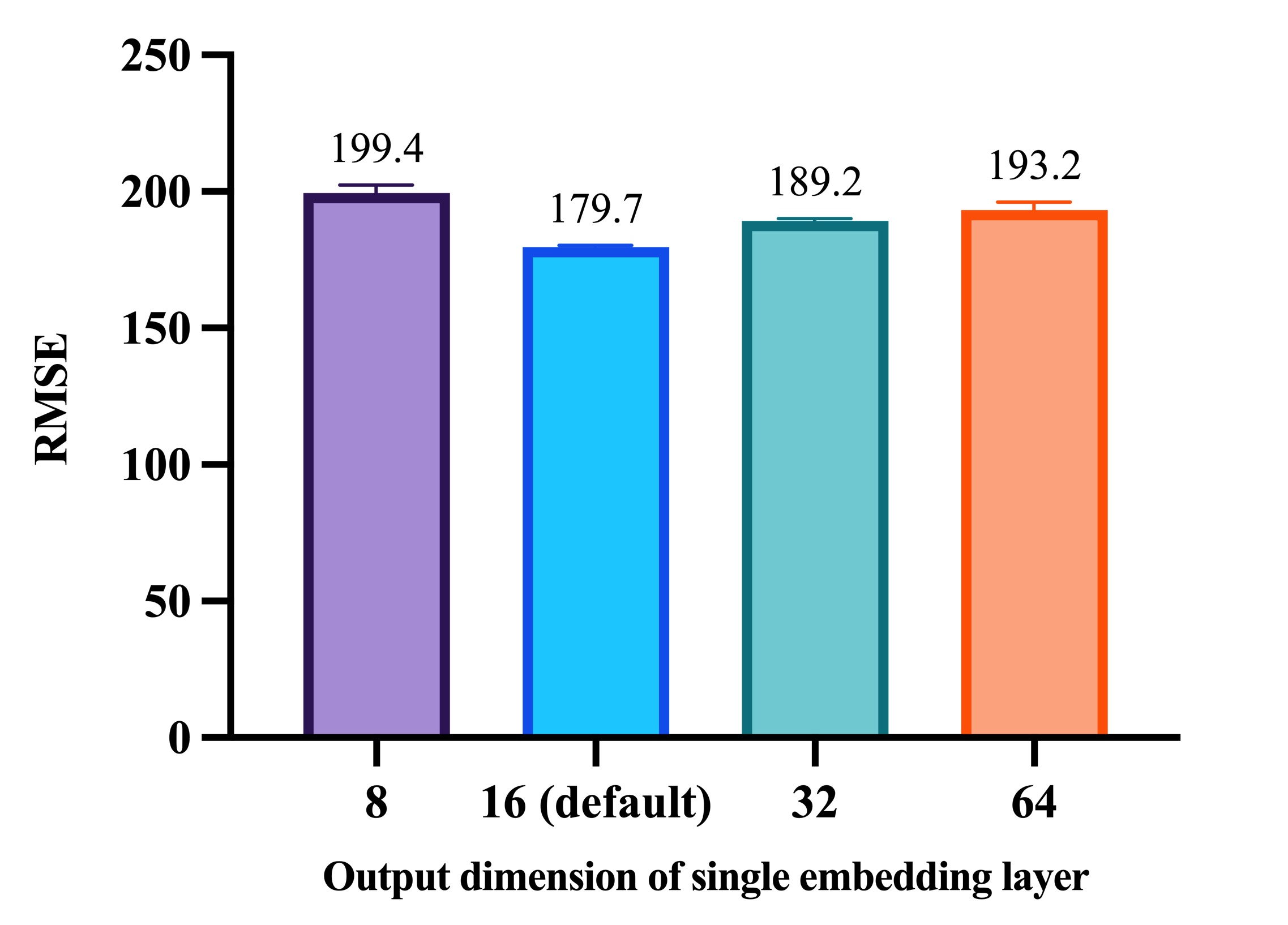
(a) Performance vs. single embedding layer

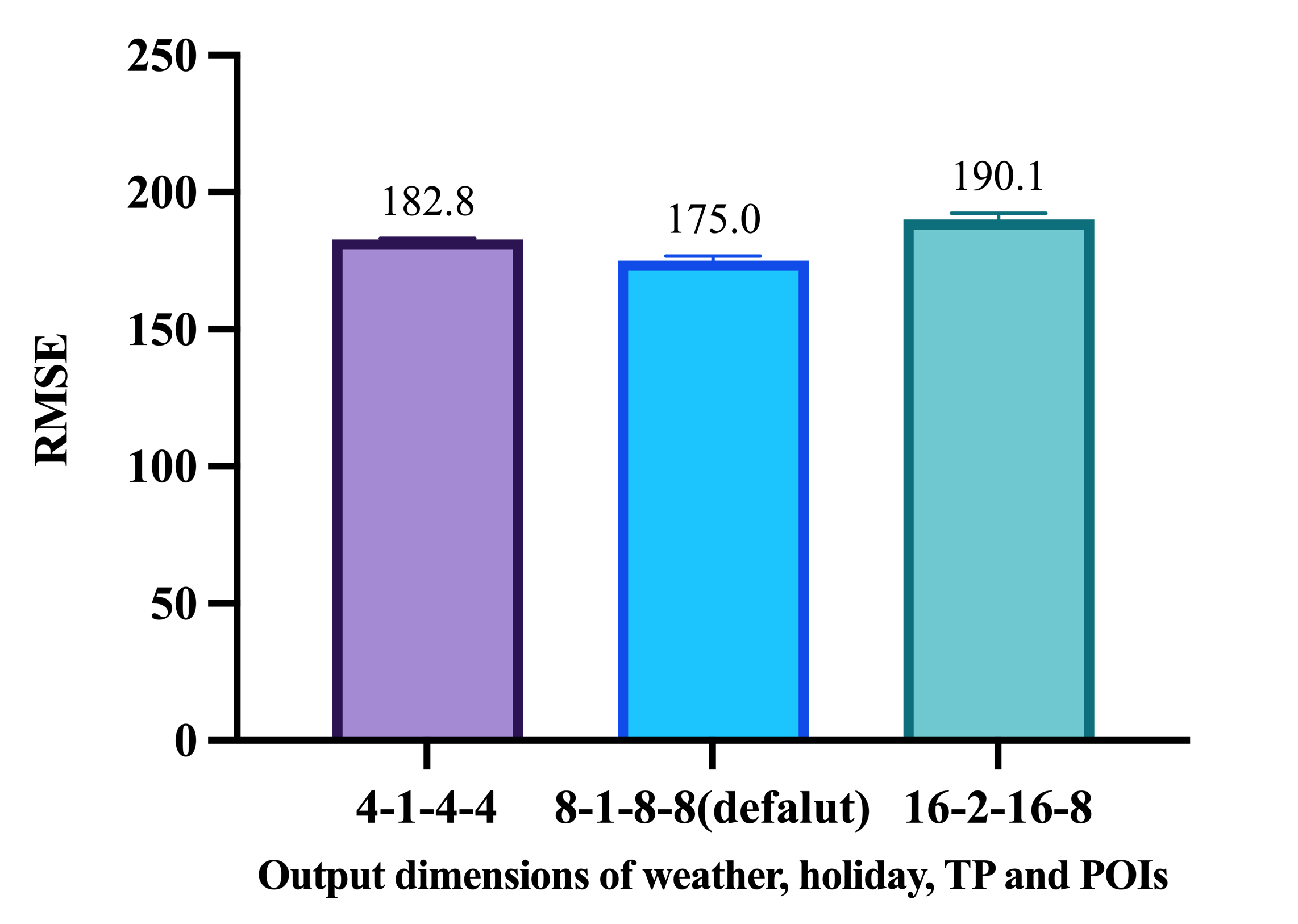
(b) Performance vs. multiple embedding layers

Figure 8: Effect of the output dimension of the single and the multiple embedding layers. These two experiments are based on Emb-Concat and MultiEmb-Concat, respectively.

Appendix D Results of Contextual Features in Different Interval Prediction Tasks

We here give the 30 and 120-minute prediction results utilizing various contextual features. The Raw-Gating method was used to combine these contextual features with the backbone model (i.e., No Context) for comparison. The 30 and 120-minute results are shown in Table X and Table XI, respectively.

TABLE X: 30-minute RMSE results of different contextual features. The best results are highlighted in bold. The feature combinations with better avgNRMSE than No Context are marked with ^∗. (Wea: Weather; Holi: Holiday; TP: Temporal Position; POIs: Point of Interest)

	XGBoost				STMGCN				STMeta
	Bike	Metro	EV	avgNRMSE	Bike	Metro	EV	avgNRMSE	Bike	Metro	EV	avgNRMSE
No Context	2.376	81.82	0.686	1.020	2.282	84.89	0.690	1.065	2.211	77.62	0.672	1.068
Wea	2.375	84.49	0.698	1.037	2.304	119.6	0.764	1.255	2.355	83.31	0.697	1.130
Holi∗	2.376	81.40	0.686	1.019∗	2.211	81.82	0.726	1.058∗	2.118	77.16	0.650	1.039∗
TP∗	2.385	80.37	0.660	1.002∗	2.218	77.29	0.672	1.013∗	2.154	71.15	0.639	1.011∗
Wea-Holi	2.376	84.55	0.697	1.037	2.217	95.74	0.756	1.134	2.271	81.50	0.652	1.085
Wea-TP	2.379	83.07	0.668	1.017∗	2.229	95.72	0.732	1.124	2.183	76.27	0.694	1.068
Holi-TP∗	2.385	80.37	0.658	1.001∗	2.229	81.08	0.687	1.039∗	2.149	72.85	0.646	1.022∗
Wea-Holi-TP	2.378	83.17	0.668	1.017∗	2.292	94.80	0.681	1.105	2.173	77.40	0.640	1.044∗
POIs	2.376	81.82	0.686	1.020	2.233	85.92	0.734	1.084	2.130	77.90	0.693	1.067∗
Wea-POIs	2.375	84.49	0.698	1.037	2.294	103.8	0.739	1.173	2.164	91.39	0.732	1.156
Holi-POIs∗	2.376	81.40	0.686	1.019∗	2.248	81.37	0.691	1.045∗	2.126	76.96	0.669	1.049∗
TP-POIs∗	2.385	80.37	0.660	1.002∗	2.155	77.12	0.722	1.028∗	2.085	71.74	0.669	1.018∗
Wea-Holi-POIs	2.376	84.55	0.697	1.037	2.290	100.3	0.757	1.166	2.170	83.93	0.669	1.089
Wea-TP-POIs	2.379	83.07	0.668	1.017∗	2.139	89.34	0.721	1.077	2.160	84.17	0.671	1.090
Holi-TP-POIs	2.385	80.37	0.658	1.001∗	2.368	82.63	0.703	1.075	2.154	76.41	0.670	1.052∗
All	2.378	83.17	0.668	1.017∗	2.152	94.46	0.709	1.095	2.106	82.38	0.680	1.077

TABLE XI: 120-minute RMSE results of different contextual features. The best results are highlighted in bold. The feature combinations with better avgNRMSE than No Context are marked with ^∗. (Wea: Weather; Holi: Holiday; TP: Temporal Position; POIs: Point of Interest)

	XGBoost				STMGCN				STMeta
	Bike	Metro	EV	avgNRMSE	Bike	Metro	EV	avgNRMSE	Bike	Metro	EV	avgNRMSE
No Context	4.121	358.6	1.089	1.022	4.334	345.5	0.965	1.051	3.830	339.6	0.955	1.078
Wea	4.061	362.5	1.137	1.036	4.142	451.2	1.091	1.181	3.792	394.5	0.947	1.129
Holi	4.084	358.2	1.134	1.033	3.977	351.2	0.965	1.026∗	3.524	338.5	0.901	1.027∗
TP∗	4.044	360.2	1.055	1.007∗	4.078	344.2	0.957	1.025∗	3.547	320.4	0.922	1.018∗
Wea-Holi	4.024	361.4	1.161	1.040	4.207	413.9	0.984	1.113	3.780	351.0	0.957	1.086
Wea-TP	3.999	363.8	1.101	1.021∗	3.935	428.3	1.001	1.109	3.647	333.5	0.931	1.045∗
Holi-TP∗	4.019	359.8	1.092	1.016∗	3.871	348.4	0.972	1.016∗	3.500	315.9	0.897	1.000∗
Wea-Holi-TP	3.985	363.4	1.139	1.031	3.844	430.7	0.985	1.098	3.741	336.9	0.906	1.048∗
POIs	4.121	358.6	1.089	1.022	3.964	366.2	0.977	1.043∗	3.922	332.4	0.942	1.074∗
Wea-POIs	4.061	362.5	1.137	1.036	4.075	415.0	1.077	1.136	3.788	362.1	0.960	1.100
Holi-POIs	4.084	358.2	1.134	1.033	3.945	366.1	0.998	1.049∗	3.893	342.7	0.914	1.072∗
TP-POIs∗	4.044	360.2	1.055	1.007∗	3.884	357.4	0.982	1.030∗	3.836	328.8	0.943	1.062∗
Wea-Holi-POIs	4.024	361.4	1.161	1.040	4.012	427.1	1.003	1.116	3.729	350.3	0.962	1.082
Wea-TP-POIs	3.999	363.8	1.101	1.021∗	3.860	419.5	1.005	1.096	3.872	348.6	0.932	1.083
Holi-TP-POIs	4.019	359.8	1.092	1.016∗	3.985	388.8	0.944	1.055	3.824	321.2	0.921	1.045∗
All	3.985	363.4	1.139	1.031	3.852	444.5	1.008	1.120	3.858	340.6	0.924	1.070∗

Appendix E Additional MAE Results

We here list the MAE results of different context modeling techniques (Table XII,XIII) and the MAE results of different combination of contextual features (Table XIV, XV, XVI).

TABLE XII: 30/60/120-minute MAE results of different modeling techniques based on STMGCN. The best results are highlighted in bold. No Context does not incorporate any contextual features.

STMGCN
	Bike			Metro			EV			avgNMAE
	30	60	120	30	60	120	30	60	120	30	60	120
No Context	1.406	1.575	2.192	40.09	74.11	124.8	0.336	0.463	0.595	1.030	1.038	1.017
Early Joint Modeling
EarlyConcat	1.397	1.576	2.216	41.04	75.10	128.5	0.328	0.481	0.605	1.027	1.057	1.037
EarlyAdd	1.395	1.582	2.239	42.00	73.12	149.0	0.327	0.471	0.633	1.034	1.041	1.113
Late Fusion
Raw-Concat	1.348	1.569	2.216	40.02	71.14	147.1	0.381	0.595	0.774	1.062	1.121	1.183
Raw-Add	1.390	1.636	2.379	47.88	81.15	169.9	0.409	0.677	0.797	1.167	1.244	1.284
Raw-Gating	1.400	1.556	2.211	40.34	76.91	120.6	0.338	0.454	0.596	1.033	1.041	1.009
Emb-Concat	1.376	1.612	2.457	41.44	71.99	148.1	0.351	0.471	0.629	1.049	1.042	1.141
Emb-Add	1.366	1.576	2.169	43.11	80.32	148.2	0.338	0.463	0.603	1.048	1.069	1.082
Emb-Gating	1.408	1.559	2.211	46.48	76.31	149.6	0.345	0.449	0.592	1.093	1.035	1.087
MultiEmb-Concat	1.375	1.571	2.219	41.44	69.10	127.5	0.351	0.468	0.654	1.049	1.017	1.061
MultiEmb-Add	1.431	1.609	2.171	43.11	75.24	136.1	0.340	0.471	0.611	1.066	1.057	1.054
MultiEmb-Gating	1.397	1.559	2.196	47.39	131.8	124.7	0.330	0.463	0.607	1.083	1.313	1.024
LSTM-Concat	1.426	1.586	2.217	49.36	107.6	233.0	0.335	0.470	0.619	1.111	1.208	1.333
LSTM-Add	1.366	1.576	2.187	45.31	79.62	148.5	0.321	0.476	0.624	1.049	1.075	1.098
LSTM-Gating	1.439	1.562	2.168	41.04	105.3	179.6	0.343	0.454	0.595	1.054	1.180	1.164

TABLE XIII: 30/60/120-minute MAE results of different modeling techniques based on STMeta. The best results are highlighted in bold. No Context does not incorporate any contextual features.

STMeta
	Bike			Metro			EV			avgNMAE
	30	60	120	30	60	120	30	60	120	30	60	120
No Context	1.374	1.648	2.093	38.37	70.48	139.4	0.342	0.461	0.604	1.048	1.051	1.068
Early Joint Modeling
EarlyConcat	1.961	1.791	2.521	64.95	135.5	227.7	0.683	0.802	0.701	1.783	1.813	1.417
EarlyAdd	1.644	1.518	2.147	39.40	70.12	159.1	0.380	0.435	0.671	1.164	1.090	1.168
Late Fusion
Raw-Concat	1.382	1.483	2.081	46.95	66.12	356.2	0.340	0.435	0.594	1.125	1.059	1.591
Raw-Add	1.417	1.491	2.053	47.27	64.90	370.3	0.366	0.515	0.645	1.163	1.116	1.653
Raw-Gating	1.394	1.457	2.061	36.51	57.98	136.0	0.338	0.434	0.558	1.031	1.006	1.026
Emb-Concat	1.372	1.490	2.063	41.32	65.02	171.5	0.345	0.437	0.554	1.076	1.056	1.110
Emb-Add	1.295	1.515	2.053	41.85	63.19	142.4	0.341	0.437	0.556	1.057	1.051	1.039
Emb-Gating	1.349	1.466	2.066	48.65	73.72	175.1	0.347	0.437	0.552	1.140	1.100	1.119
MultiEmb-Concat	1.350	1.451	2.062	42.27	68.45	145.9	0.342	0.470	0.590	1.076	1.092	1.070
MultiEmb-Add	1.458	1.494	2.060	49.72	66.99	181.5	0.342	0.432	0.584	1.172	1.064	1.153
MultiEmb-Gating	1.360	1.502	2.063	43.45	130.0	169.0	0.342	0.432	0.530	1.090	1.429	1.089
LSTM-Concat	1.380	1.456	2.070	38.86	65.09	150.4	0.340	0.438	0.556	1.051	1.049	1.061
LSTM-Add	1.334	1.440	2.064	38.92	63.44	141.7	0.332	0.437	0.551	1.032	1.045	1.036
LSTM-Gating	1.390	1.450	2.012	39.40	61.91	147.7	0.333	0.436	0.556	1.051	1.028	1.045

TABLE XIV: 30-minute MAE results of different contextual features. The best results are highlighted in bold. (Wea: Weather; Holi: Holiday; TP: Temporal Position; POIs: Point of Interest)

	XGBoost				STMGCN				STMeta
	Bike	Metro	EV	avgNMAE	Bike	Metro	EV	avgNMAE	Bike	Metro	EV	avgNMAE
No Context	1.532	39.41	0.336	1.016	1.406	40.09	0.336	1.049	1.374	38.37	0.342	1.057
Wea	1.516	41.26	0.357	1.048	1.407	58.95	0.401	1.285	1.452	41.99	0.337	1.105
Holi	1.532	39.24	0.338	1.016	1.415	40.09	0.433	1.150	1.359	37.54	0.331	1.033
TP	1.543	39.10	0.327	1.006	1.410	37.23	0.328	1.011	1.382	35.98	0.325	1.018
Wea-Holi	1.516	41.22	0.356	1.048	1.370	49.97	0.428	1.223	1.467	40.50	0.339	1.096
Wea-TP	1.524	40.81	0.341	1.030	1.352	47.86	0.390	1.161	1.393	39.62	0.336	1.066
Holi-TP	1.543	39.09	0.327	1.006	1.382	39.23	0.358	1.058	1.38	36.62	0.324	1.023
Wea-Holi-TP	1.523	40.79	0.341	1.030	1.400	48.34	0.338	1.125	1.394	39.51	0.328	1.057
POIs	1.532	39.41	0.336	1.016	1.411	42.50	0.422	1.160	1.361	38.10	0.335	1.043
Wea-POIs	1.516	41.26	0.357	1.048	1.396	51.46	0.377	1.191	1.381	50.58	0.369	1.201
Holi-POIs	1.532	39.24	0.338	1.016	1.415	39.80	0.370	1.084	1.361	37.72	0.344	1.049
TP-POIs	1.543	39.10	0.327	1.006	1.392	37.96	0.383	1.075	1.333	35.41	0.344	1.020
Wea-Holi-POIs	1.516	41.22	0.356	1.048	1.404	53.70	0.449	1.286	1.368	42.70	0.344	1.097
Wea-TP-POIs	1.524	40.81	0.341	1.030	1.345	44.62	0.392	1.132	1.385	42.71	0.342	1.100
Holi-TP-POIs	1.543	39.09	0.327	1.006	1.449	39.08	0.374	1.090	1.361	38.45	0.325	1.036
All	1.523	40.79	0.341	1.030	1.345	48.09	0.378	1.149	1.365	41.14	0.344	1.082

TABLE XV: 60-minute MAE results of different contextual features. The best results are highlighted in bold. (Wea: Weather; Holi: Holiday; TP: Temporal Position; POIs: Point of Interest)

	XGBoost				STMGCN				STMeta
	Bike	Metro	EV	avgNMAE	Bike	Metro	EV	avgNMAE	Bike	Metro	EV	avgNMAE
No Context	1.737	71.33	0.458	1.026	1.575	74.11	0.463	1.024	1.648	70.48	0.461	1.113
Wea	1.716	74.51	0.480	1.054	1.605	99.01	0.483	1.157	1.579	76.94	0.468	1.138
Holi	1.721	71.30	0.458	1.023	1.602	79.82	0.460	1.053	1.551	69.62	0.442	1.072
TP	1.707	71.10	0.440	1.006	1.587	86.93	0.451	1.075	1.491	61.14	0.457	1.023
Wea-Holi	1.701	74.13	0.480	1.049	1.614	110.1	0.504	1.225	1.553	77.53	0.453	1.124
Wea-TP	1.688	74.02	0.457	1.028	1.562	104.4	0.465	1.159	1.471	71.21	0.442	1.062
Holi-TP	1.700	71.21	0.439	1.004	1.599	77.35	0.440	1.026	1.472	60.36	0.439	1.000
Wea-Holi-TP	1.683	73.95	0.456	1.026	1.546	100.4	0.454	1.129	1.503	71.38	0.452	1.078
POIs	1.737	71.33	0.458	1.026	1.592	74.47	0.503	1.059	1.580	67.46	0.444	1.068
Wea-POIs	1.716	74.51	0.480	1.054	1.550	114.7	0.463	1.201	1.597	84.98	0.468	1.187
Holi-POIs	1.721	71.30	0.458	1.023	1.593	79.36	0.457	1.047	1.577	67.82	0.442	1.068
TP-POIs	1.707	71.10	0.440	1.006	1.571	77.32	0.459	1.034	1.534	62.24	0.444	1.028
Wea-Holi-POIs	1.701	74.13	0.480	1.049	1.561	110.5	0.522	1.229	1.573	82.06	0.460	1.159
Wea-TP-POIs	1.688	74.02	0.457	1.028	1.591	113.2	0.469	1.207	1.537	84.77	0.458	1.164
Holi-TP-POIs	1.700	71.21	0.439	1.004	1.561	78.62	0.457	1.036	1.542	62.48	0.445	1.032
All	1.683	73.95	0.456	1.026	1.573	102.8	0.456	1.147	1.538	72.47	0.452	1.092

TABLE XVI: 120-minute MAE results of different contextual features. The best results are highlighted in bold. (Wea: Weather; Holi: Holiday; TP: Temporal Position; POIs: Point of Interest)

	XGBoost				STMGCN				STMeta
	Bike	Metro	EV	avgNMAE	Bike	Metro	EV	avgNMAE	Bike	Metro	EV	avgNMAE
No Context	2.246	137.6	0.695	1.032	2.192	124.8	0.595	1.032	2.093	139.4	0.604	1.144
Wea	2.218	139.5	0.728	1.049	2.259	185.4	0.741	1.291	2.072	189.9	0.596	1.277
Holi	2.228	137.1	0.695	1.028	2.176	130.5	0.590	1.042	1.903	138.4	0.551	1.074
TP	2.211	138.1	0.655	1.007	2.161	123.1	0.584	1.017	1.922	122.1	0.571	1.045
Wea-Holi	2.201	139.7	0.727	1.046	2.219	164.3	0.616	1.156	2.068	148.4	0.606	1.166
Wea-TP	2.186	139.9	0.694	1.028	2.155	174.1	0.605	1.166	1.969	133.0	0.579	1.089
Holi-TP	2.201	137.7	0.655	1.005	2.173	126.9	0.601	1.038	1.898	119.0	0.521	1.000
Wea-Holi-TP	2.178	139.8	0.694	1.027	2.211	170.6	0.596	1.160	2.021	136.0	0.558	1.093
POIs	2.246	137.6	0.695	1.032	2.126	148.4	0.581	1.078	2.158	133.6	0.592	1.132
Wea-POIs	2.218	139.5	0.728	1.049	2.302	165.6	0.731	1.239	2.084	157.9	0.611	1.199
Holi-POIs	2.228	137.1	0.695	1.028	2.165	142.9	0.621	1.092	2.145	142.8	0.564	1.137
TP-POIs	2.211	138.1	0.655	1.007	2.136	134.6	0.620	1.064	2.128	137.9	0.594	1.139
Wea-Holi-POIs	2.201	139.7	0.727	1.046	2.207	168.2	0.611	1.162	2.066	148.1	0.612	1.169
Wea-TP-POIs	2.186	139.9	0.694	1.028	2.135	164.5	0.636	1.154	2.148	145.1	0.581	1.155
Holi-TP-POIs	2.201	137.7	0.655	1.005	2.211	148.4	0.579	1.090	2.139	120.9	0.571	1.079
All	2.178	139.8	0.694	1.027	2.075	182.0	0.611	1.178	2.146	139.2	0.574	1.134

References

- [1] L. Wang, X. Geng, X. Ma, D. Zhang, and Q. Yang, “Ridesharing car detection by transfer learning,” Artif. Intell., p. 1–18, aug 2019.
- [2] R. Al Mallah, A. Quintero, and B. Farooq, “Prediction of traffic flow via connected vehicles,” IEEE Transactions on Mobile Computing, vol. 21, no. 1, pp. 264–277, 2022.
- [3] J. Zhang and X. Zhang, “Multi-task allocation in mobile crowd sensing with mobility prediction,” IEEE Transactions on Mobile Computing, vol. 22, no. 2, pp. 1081–1094, 2023.
- [4] H. Li, F. Lin, X. Lu, C. Xu, G. Huang, J. Zhang, Q. Mei, and X. Liu, “Systematic analysis of fine-grained mobility prediction with on-device contextual data,” IEEE Transactions on Mobile Computing, vol. 21, no. 3, pp. 1096–1109, 2022.
- [5] M. Lv, D. Zeng, L. Chen, T. Chen, T. Zhu, and S. Ji, “Private cell-id trajectory prediction using multi-graph embedding and encoder-decoder network,” IEEE Transactions on Mobile Computing, vol. 21, no. 8, pp. 2967–2977, 2022.
- [6] L. Chen, T.-M.-T. Nguyen, D. Yang, M. Nogueira, C. Wang, and D. Zhang, “Data-driven c-ran optimization exploiting traffic and mobility dynamics of mobile users,” IEEE Transactions on Mobile Computing, vol. 20, no. 5, pp. 1773–1788, 2021.
- [7] L. Yu, M. Li, W. Jin, Y. Guo, Q. Wang, F. Yan, and P. Li, “Step: A spatio-temporal fine-granular user traffic prediction system for cellular networks,” IEEE Transactions on Mobile Computing, vol. 20, no. 12, pp. 3453–3466, 2021.
- [8] K. He, X. Chen, Q. Wu, S. Yu, and Z. Zhou, “Graph attention spatial-temporal network with collaborative global-local learning for citywide mobile traffic prediction,” IEEE Transactions on Mobile Computing, vol. 21, no. 4, pp. 1244–1256, 2022.
- [9] H. Zhu, T. Shou, R. Guo, Z. Jiang, Z. Wang, Z. Wang, Z. Yu, W. Zhang, C. Wang, and L. Chen, “Redpacketbike: A graph-based demand modeling and crowd-driven station rebalancing framework for bike sharing systems,” IEEE Transactions on Mobile Computing, vol. 22, no. 7, pp. 4236–4252, 2023.
- [10] F. Sun, P. Wang, J. Zhao, N. Xu, J. Zeng, J. Tao, K. Song, C. Deng, J. C. Lui, and X. Guan, “Mobile data traffic prediction by exploiting time-evolving user mobility patterns,” IEEE Transactions on Mobile Computing, vol. 21, no. 12, pp. 4456–4470, 2022.
- [11] Y. Yao, B. Gu, Z. Su, and M. Guizani, “Mvstgn: A multi-view spatial-temporal graph network for cellular traffic prediction,” IEEE Transactions on Mobile Computing, vol. 22, no. 5, pp. 2837–2849, 2023.
- [12] Y. Yuan, D. Zhang, F. Miao, J. A. Stankovic, T. He, G. J. Pappas, and S. Lin, “: Mobility-driven integration of heterogeneous urban cyber-physical systems under disruptive events,” IEEE Transactions on Mobile Computing, vol. 22, no. 2, pp. 906–922, 2023.
- [13] B. Guo, J. Li, V. W. Zheng, Z. Wang, and Z. Yu, “Citytransfer: Transferring inter- and intra-city knowledge for chain store site recommendation based on multi-source urban data,” Proc. ACM Interact. Mob. Wearable Ubiquitous Technol., 2018.
- [14] Y. Li, Y. Zheng, H. Zhang, and L. Chen, “Traffic prediction in a bike-sharing system,” in Proceedings of the 23rd SIGSPATIAL International Conference on Advances in Geographic Information Systems, 2015, pp. 1–10.
- [15] Z. Yang, J. Hu, Y. Shu, P. Cheng, J. Chen, and T. Moscibroda, “Mobility Modeling and Prediction in Bike-Sharing Systems,” in Proceedings of the 14th Annual International Conference on Mobile Systems, Applications, and Services, 2016, pp. 165–178.
- [16] D. Chai, L. Wang, and Q. Yang, “Bike flow prediction with multi-graph convolutional networks,” in Proceedings of the 26th ACM SIGSPATIAL International Conference on Advances in Geographic Information Systems, ser. SIGSPATIAL ’18. New York, NY, USA: Association for Computing Machinery, 2018, p. 397–400.
- [17] Y. Li and Y. Zheng, “Citywide bike usage prediction in a bike-sharing system,” IEEE Transactions on Knowledge and Data Engineering, vol. 32, no. 6, pp. 1079–1091, 2020.
- [18] Y. Tong, Y. Chen, Z. Zhou, L. Chen, J. Wang, Q. Yang, J. Ye, and W. Lv, “The Simpler The Better: A Unified Approach to Predicting Original Taxi Demands based on Large-Scale Online Platforms,” in Proceedings of the 23rd ACM SIGKDD International Conference on Knowledge Discovery and Data Mining, 2017, pp. 1653–1662.
- [19] J. Ke, H. Zheng, H. Yang, and X. M. Chen, “Short-term forecasting of passenger demand under on-demand ride services: A spatio-temporal deep learning approach,” Transportation Research Part C: Emerging Technologies, vol. 85, pp. 591–608, 2017.
- [20] D. Wang, W. Cao, J. Li, and J. Ye, “DeepSD: Supply-Demand Prediction for Online Car-Hailing Services Using Deep Neural Networks,” in 2017 IEEE 33rd International Conference on Data Engineering, 2017, pp. 243–254.
- [21] L. Zhu and N. Laptev, “Deep and confident prediction for time series at uber,” in 2017 IEEE International Conference on Data Mining Workshops (ICDMW), 2017, pp. 103–110.
- [22] H. Yao, F. Wu, J. Ke, X. Tang, Y. Jia, S. Lu, P. Gong, J. Ye, and Z. Li, “Deep multi-view spatial-temporal network for taxi demand prediction,” Proceedings of the AAAI Conference on Artificial Intelligence, vol. 32, no. 1, 2018.
- [23] A. Saadallah, L. Moreira-Matias, R. Sousa, J. Khiari, E. Jenelius, and J. Gama, “Bright—drift-aware demand predictions for taxi networks,” IEEE Transactions on Knowledge and Data Engineering, vol. 32, no. 2, pp. 234–245, 2020.
- [24] Y. Li, R. Yu, C. Shahabi, and Y. Liu, “Diffusion convolutional recurrent neural network: Data-driven traffic forecasting,” in International Conference on Learning Representations (ICLR ’18), 2018.
- [25] X. Yi, Z. Duan, T. Li, T. Li, J. Zhang, and Y. Zheng, “Citytraffic: Modeling citywide traffic via neural memorization and generalization approach,” in Proceedings of the 28th ACM International Conference on Information and Knowledge Management, 2019, pp. 2665–2671.
- [26] J. Zhang, Y. Zheng, and D. Qi, “Deep spatio-temporal residual networks for citywide crowd flows prediction,” in Proceedings of the Thirty-First AAAI Conference on Artificial Intelligence, 2017, p. 1655–1661.
- [27] J. Chu, X. Wang, K. Qian, L. Yao, F. Xiao, J. Li, and Z. Yang, “Passenger demand prediction with cellular footprints,” IEEE Transactions on Mobile Computing, vol. 21, no. 01, pp. 252–263, 2022.
- [28] M. X. Hoang, Y. Zheng, and A. K. Singh, “Fccf: Forecasting citywide crowd flows based on big data,” in Proceedings of the 24th ACM SIGSPATIAL International Conference on Advances in Geographic Information Systems, 2016.
- [29] G. D. Abowd, A. K. Dey, P. J. Brown, N. Davies, M. Smith, and P. Steggles, “Towards a better understanding of context and context-awareness,” in International symposium on handheld and ubiquitous computing, 1999, pp. 304–307.
- [30] F. Xu, P. Zhang, and Y. Li, “Context-aware real-time population estimation for metropolis,” in Proceedings of the 2016 ACM International Joint Conference on Pervasive and Ubiquitous Computing, 2016, pp. 1064–1075.
- [31] Z. Lin, J. Feng, Z. Lu, Y. Li, and D. Jin, “Deepstn+: Context-aware spatial-temporal neural network for crowd flow prediction in metropolis,” Proceedings of the AAAI Conference on Artificial Intelligence, vol. 33, no. 01, pp. 1020–1027, 2019.
- [32] Y. Liang, S. Ke, J. Zhang, X. Yi, and Y. Zheng, “GeoMAN: Multi-level Attention Networks for Geo-sensory Time Series Prediction,” in Proceedings of the Twenty-Seventh International Joint Conference on Artificial Intelligence, 2018, pp. 3428–3434.
- [33] S. Guo, Y. Lin, N. Feng, C. Song, and H. Wan, “Attention based spatial-temporal graph convolutional networks for traffic flow forecasting,” Proceedings of the AAAI Conference on Artificial Intelligence, vol. 33, no. 01, pp. 922–929, Jul. 2019.
- [34] C. Zheng, X. Fan, C. Wang, and J. Qi, “Gman: A graph multi-attention network for traffic prediction,” in Proceedings of the AAAI conference on artificial intelligence, vol. 34, no. 01, 2020, pp. 1234–1241.
- [35] B. Yu, H. Yin, and Z. Zhu, “Spatio-temporal graph convolutional networks: A deep learning framework for traffic forecasting,” in Proceedings of the 27th International Joint Conference on Artificial Intelligence, 2018.
- [36] L. Wang, X. Geng, X. Ma, F. Liu, and Q. Yang, “Cross-city transfer learning for deep spatio-temporal prediction,” in Proceedings of the Twenty-Eighth International Joint Conference on Artificial Intelligence, 2019, pp. 1893–1899.
- [37] X. Wang, Z. Zhou, Y. Zhao, X. Zhang, K. Xing, F. Xiao, Z. Yang, and Y. Liu, “Improving urban crowd flow prediction on flexible region partition,” IEEE Transactions on Mobile Computing, vol. 19, no. 12, pp. 2804–2817, 2020.
- [38] X. Fan, C. Xiang, C. Chen, P. Yang, L. Gong, X. Song, P. Nanda, and X. He, “Buildsensys: Reusing building sensing data for traffic prediction with cross-domain learning,” IEEE Transactions on Mobile Computing, vol. 20, no. 6, pp. 2154–2171, 2021.
- [39] L. Wang, D. Chai, X. Liu, L. Chen, and K. Chen, “Exploring the generalizability of spatio-temporal traffic prediction: Meta-modeling and an analytic framework,” IEEE Transactions on Knowledge and Data Engineering, pp. 1–1, 2021.
- [40] J. Zhang, Y. Zheng, D. Qi, R. Li, and X. Yi, “Dnn-based prediction model for spatio-temporal data,” in Proceedings of the 24th ACM SIGSPATIAL International Conference on Advances in Geographic Information Systems, 2016, pp. 1–4.
- [41] J. Zhang, Y. Zheng, J. Sun, and D. Qi, “Flow Prediction in Spatio-Temporal Networks Based on Multitask Deep Learning,” IEEE Transactions on Knowledge and Data Engineering, pp. 1–1, 2019.
- [42] Y. Liu, Z. Liu, and R. Jia, “DeepPF: A deep learning based architecture for metro passenger flow prediction,” Transportation Research Part C: Emerging Technologies, vol. 101, pp. 18–34, 2019.
- [43] J. Ou, J. Sun, Y. Zhu, H. Jin, Y. Liu, F. Zhang, J. Huang, and X. Wang, “Stp-trellisnets+: Spatial-temporal parallel trellisnets for multi-step metro station passenger flow prediction,” IEEE Transactions on Knowledge and Data Engineering, pp. 1–14, 2022.
- [44] D. Yin, R. Jiang, J. Deng, Y. Li, Y. Xie, Z. Wang, Y. Zhou, X. Song, and J. S. Shang, “Mtmgnn: Multi-time multi-graph neural network for metro passenger flow prediction,” GeoInformatica, vol. 27, no. 1, pp. 77–105, 2023.
- [45] J. Sun, J. Zhang, Q. Li, X. Yi, Y. Liang, and Y. Zheng, “Predicting citywide crowd flows in irregular regions using multi-view graph convolutional networks,” IEEE Transactions on Knowledge and Data Engineering, vol. PP, pp. 1–1, 07 2020.
- [46] H. Yuan, G. Li, Z. Bao, and L. Feng, “An effective joint prediction model for travel demands and traffic flows,” in 2021 IEEE 37th International Conference on Data Engineering, 2021, pp. 348–359.
- [47] X. Zhang, C. Huang, Y. Xu, L. Xia, P. Dai, L. Bo, J. Zhang, and Y. Zheng, “Traffic flow forecasting with spatial-temporal graph diffusion network,” Proceedings of the AAAI Conference on Artificial Intelligence, vol. 35, no. 17, pp. 15 008–15 015, 2021.
- [48] Z. Wu, S. Pan, G. Long, J. Jiang, and C. Zhang, “Graph wavenet for deep spatial-temporal graph modeling,” in Proceedings of the 28th International Joint Conference on Artificial Intelligence, 2019, p. 1907–1913.
- [49] L. Bai, L. Yao, C. Li, X. Wang, and C. Wang, “Adaptive graph convolutional recurrent network for traffic forecasting,” in Proceedings of the 34th International Conference on Neural Information Processing Systems, ser. NIPS’20. Red Hook, NY, USA: Curran Associates Inc., 2020.
- [50] C. Zheng, X. Fan, C. Wang, and J. Qi, “Gman: A graph multi-attention network for traffic prediction,” Proceedings of the AAAI Conference on Artificial Intelligence, vol. 34, no. 01, pp. 1234–1241, 2020.
- [51] R. Barnes, S. Buthpitiya, J. Cook, A. Fabrikant, A. Tomkins, and F. Xu, “Bustr: Predicting bus travel times from real-time traffic,” in The 26th ACM SIGKDD Conference on Knowledge Discovery and Data Mining, 2020, pp. 3243–3251.
- [52] C. Zheng, X. Fan, C. Wen, L. Chen, C. Wang, and J. Li, “Deepstd: Mining spatio-temporal disturbances of multiple context factors for citywide traffic flow prediction,” IEEE Transactions on Intelligent Transportation Systems, vol. 21, no. 9, pp. 3744–3755, 2020.
- [53] C. Chen, K. Li, S. G. Teo, X. Zou, K. Li, and Z. Zeng, “Citywide traffic flow prediction based on multiple gated spatio-temporal convolutional neural networks,” ACM Trans. Knowl. Discov. Data, vol. 14, no. 4, may 2020.
- [54] A. Zonoozi, J. jae Kim, X.-L. Li, and G. Cong, “Periodic-crn: A convolutional recurrent model for crowd density prediction with recurring periodic patterns,” in Proceedings of the Twenty-Seventh International Joint Conference on Artificial Intelligence, 7 2018, pp. 3732–3738.
- [55] K. Chen, F. Chen, B. Lai, Z. Jin, Y. Liu, K. Li, L. Wei, P. Wang, Y. Tang, J. Huang, and X. S. Hua, “Dynamic spatio-temporal graph-based cnns for traffic flow prediction,” IEEE Access, vol. 8, pp. 185 136–185 145, 2020.
- [56] R. Jiang, Z. Cai, Z. Wang, C. Yang, Z. Fan, Q. Chen, K. Tsubouchi, X. Song, and R. Shibasaki, “Deepcrowd: A deep model for large-scale citywide crowd density and flow prediction,” IEEE Transactions on Knowledge and Data Engineering, pp. 1–1, 2021.
- [57] Y. Liang, K. Ouyang, J. Sun, Y. Wang, J. Zhang, Y. Zheng, D. Rosenblum, and R. Zimmermann, “Fine-grained urban flow prediction,” in Proceedings of the Web Conference 2021, 2021, p. 1833–1845.
- [58] F. Wu, H. Wang, and Z. Li, “Interpreting traffic dynamics using ubiquitous urban data,” in Proceedings of the 24th ACM SIGSPATIAL International Conference on Advances in Geographic Information Systems, 2016.
- [59] G. Atluri, A. Karpatne, and V. Kumar, “Spatio-temporal data mining: A survey of problems and methods,” ACM Comput. Surv., vol. 51, no. 4, aug 2018.
- [60] N. J. Yuan, Y. Zheng, X. Xie, Y. Wang, K. Zheng, and H. Xiong, “Discovering urban functional zones using latent activity trajectories,” IEEE Transactions on Knowledge and Data Engineering, vol. 27, no. 3, pp. 712–725, 2014.
- [61] S. Ling, Z. Yu, S. Cao, H. Zhang, and S. Hu, “Sthan: Transportation demand forecasting with compound spatio-temporal relationships,” ACM Trans. Knowl. Discov. Data, oct 2022.
- [62] N. J. Yuan, Y. Zheng, X. Xie, Y. Wang, K. Zheng, and H. Xiong, “Discovering urban functional zones using latent activity trajectories,” IEEE Transactions on Knowledge and Data Engineering, vol. 27, no. 3, pp. 712–725, 2015.
- [63] J. Ye, L. Sun, B. Du, Y. Fu, X. Tong, and H. Xiong, “Co-prediction of multiple transportation demands based on deep spatio-temporal neural network,” in Proceedings of the 25th ACM SIGKDD International Conference on Knowledge Discovery and Data Mining, 2019, p. 305–313.
- [64] Z. Pan, Y. Liang, W. Wang, Y. Yu, Y. Zheng, and J. Zhang, “Urban traffic prediction from spatio-temporal data using deep meta learning,” in Proceedings of the 25th ACM SIGKDD International Conference on Knowledge Discovery and Data Mining, 2019, p. 1720–1730.
- [65] Z. Fang, Q. Long, G. Song, and K. Xie, “Spatial-temporal graph ode networks for traffic flow forecasting,” in Proceedings of the 27th ACM SIGKDD Conference on Knowledge Discovery and Data Mining, 2021, p. 364–373.
- [66] S. Hochreiter and J. Schmidhuber, “Long short-term memory,” Neural computation, vol. 9, no. 8, pp. 1735–1780, 1997.
- [67] Y. N. Dauphin, A. Fan, M. Auli, and D. Grangier, “Language modeling with gated convolutional networks,” in Proceedings of the 34th International Conference on Machine Learning - Volume 70, 2017, p. 933–941.
- [68] M. Xu, W. Dai, C. Liu, X. Gao, W. Lin, G.-J. Qi, and H. Xiong, “Spatial-temporal transformer networks for traffic flow forecasting,” arXiv preprint arXiv:2001.02908, 2020.
- [69] T. N. Kipf and M. Welling, “Semi-supervised classification with graph convolutional networks,” in International Conference on Learning Representations, 2017.
- [70] P. Veličković, G. Cucurull, A. Casanova, A. Romero, P. Liò, and Y. Bengio, “Graph attention networks,” International Conference on Learning Representations, 2018.
- [71] X. SHI, Z. Chen, H. Wang, D.-Y. Yeung, W.-k. Wong, and W.-c. WOO, “Convolutional lstm network: A machine learning approach for precipitation nowcasting,” in Advances in Neural Information Processing Systems, C. Cortes, N. Lawrence, D. Lee, M. Sugiyama, and R. Garnett, Eds., vol. 28. Curran Associates, Inc., 2015.
- [72] T. Chen and C. Guestrin, “Xgboost: A scalable tree boosting system,” in Proceedings of the 22nd ACM SIGKDD International Conference on Knowledge Discovery and Data Mining, 2016, p. 785–794.
- [73] J. Feng, Y. Li, Z. Lin, C. Rong, F. Sun, D. Guo, and D. Jin, “Context-aware spatial-temporal neural network for citywide crowd flow prediction via modeling long-range spatial dependency,” ACM Trans. Knowl. Discov. Data, vol. 16, no. 3, oct 2021.
- [74] H. Yao, X. Tang, H. Wei, G. Zheng, Y. Yu, and Z. Li, “Modeling spatial-temporal dynamics for traffic prediction,” ArXiv, vol. abs/1803.01254, 2018.
- [75] X. Geng, Y. Li, L. Wang, L. Zhang, Q. Yang, J. Ye, and Y. Liu, “Spatiotemporal multi-graph convolution network for ride-hailing demand forecasting,” Proceedings of the AAAI Conference on Artificial Intelligence, vol. 33, no. 01, pp. 3656–3663, 2019.
- [76] F. Li, J. Feng, H. Yan, G. Jin, F. Yang, F. Sun, D. Jin, and Y. Li, “Dynamic graph convolutional recurrent network for traffic prediction: Benchmark and solution,” ACM Trans. Knowl. Discov. Data, 2023.
- [77] M. M. Hamed, H. R. Al-Masaeid, and Z. M. B. Said, “Short-term prediction of traffic volume in urban arterials,” Journal of Transportation Engineering, vol. 121, no. 3, pp. 249–254, 1995.
- [78] Y. Cong, J. Wang, and X. Li, “Traffic flow forecasting by a least squares support vector machine with a fruit fly optimization algorithm,” Procedia Engineering, vol. 137, no. 1, pp. 59–68, 2016.
- [79] J. Wang, W. Deng, and Y. Guo, “New bayesian combination method for short-term traffic flow forecasting,” Transportation Research Part C: Emerging Technologies, vol. 43, pp. 79–94, 2014.
- [80] J. Chung, C. Gulcehre, K. Cho, and Y. Bengio, “Empirical evaluation of gated recurrent neural networks on sequence modeling,” arXiv preprint arXiv:1412.3555, 2014.
- [81] A. van den Oord, S. Dieleman, H. Zen, K. Simonyan, O. Vinyals, A. Graves, N. Kalchbrenner, A. Senior, and K. Kavukcuoglu, “Wavenet: A generative model for raw audio,” in Arxiv, 2016.
- [82] H. Zhou, S. Zhang, J. Peng, S. Zhang, J. Li, H. Xiong, and W. Zhang, “Informer: Beyond efficient transformer for long sequence time-series forecasting,” in The Thirty-Fifth AAAI Conference on Artificial Intelligence, AAAI 2021, Virtual Conference, vol. 35, no. 12, 2021, pp. 11 106–11 115.
- [83] H. Wu, J. Xu, J. Wang, and M. Long, “Autoformer: Decomposition transformers with Auto-Correlation for long-term series forecasting,” in Advances in Neural Information Processing Systems, 2021.
- [84] T. Zhou, Z. Ma, Q. Wen, X. Wang, L. Sun, and R. Jin, “FEDformer: Frequency enhanced decomposed transformer for long-term series forecasting,” in Proceedings of the 39th International Conference on Machine Learning, vol. 162, 2022, pp. 27 268–27 286.
- [85] Y. Liu, H. Wu, J. Wang, and M. Long, “Non-stationary transformers: Exploring the stationarity in time series forecasting,” in Advances in Neural Information Processing Systems, 2022.
- [86] Y. Zhang, Y. Li, X. Zhou, X. Kong, and J. Luo, “Curb-gan: Conditional urban traffic estimation through spatio-temporal generative adversarial networks,” in Proceedings of the 26th ACM SIGKDD International Conference on Knowledge Discovery and Data Mining, 2020, p. 842–852.
- [87] C. Song, Y. Lin, S. Guo, and H. Wan, “Spatial-temporal synchronous graph convolutional networks: A new framework for spatial-temporal network data forecasting,” in Proceedings of the AAAI conference on artificial intelligence, vol. 34, no. 01, 2020, pp. 914–921.
- [88] L. Han, B. Du, L. Sun, Y. Fu, Y. Lv, and H. Xiong, “Dynamic and multi-faceted spatio-temporal deep learning for traffic speed forecasting,” in Proceedings of the 27th ACM SIGKDD Conference on Knowledge Discovery and Data Mining, 2021, p. 547–555.
- [89] H. qin, X. Zhan, Y. Li, X. Yang, and Y. Zheng, “Network-wide traffic states imputation using self-interested coalitional learning,” in Proceedings of the 27th ACM SIGKDD Conference on Knowledge Discovery and Data Mining, 2021, p. 1370–1378.
- [90] Z. Shao, Z. Zhang, W. Wei, F. Wang, Y. Xu, X. Cao, and C. S. Jensen, “Decoupled dynamic spatial-temporal graph neural network for traffic forecasting,” Proc. VLDB Endow., vol. 15, no. 11, p. 2733–2746, sep 2022.
- [91] X. Lei, H. Mei, B. Shi, and H. Wei, “Modeling network-level traffic flow transitions on sparse data,” in Proceedings of the 28th ACM SIGKDD Conference on Knowledge Discovery and Data Mining, 2022, p. 835–845.
- [92] D. Liu, J. Wang, S. Shang, and P. Han, “Msdr: Multi-step dependency relation networks for spatial temporal forecasting,” in Proceedings of the 28th ACM SIGKDD Conference on Knowledge Discovery and Data Mining, 2022, p. 1042–1050.
- [93] Z. Shao, Z. Zhang, F. Wang, and Y. Xu, “Pre-training enhanced spatial-temporal graph neural network for multivariate time series forecasting,” in Proceedings of the 28th ACM SIGKDD Conference on Knowledge Discovery and Data Mining, 2022, p. 1567–1577.
- [94] H. Lin, R. Bai, W. Jia, X. Yang, and Y. You, “Preserving dynamic attention for long-term spatial-temporal prediction,” in Proceedings of the 26th ACM SIGKDD International Conference on Knowledge Discovery and Data Mining, 2020, p. 36–46.
- [95] B. Hui, D. Yan, H. Chen, and W.-S. Ku, “Trajnet: A trajectory-based deep learning model for traffic prediction,” in Proceedings of the 27th ACM SIGKDD Conference on Knowledge Discovery and Data Mining, 2021, p. 716–724.
- [96] F. Li, J. Feng, H. Yan, D. Jin, and Y. Li, “Crowd flow prediction for irregular regions with semantic graph attention network,” ACM Trans. Intell. Syst. Technol., 2022.
- [97] S. Wang, J. Cao, and P. Yu, “Deep learning for spatio-temporal data mining: A survey,” IEEE Transactions on Knowledge and Data Engineering, pp. 1–1, 2020.
- [98] R. Jiang, D. Yin, Z. Wang, Y. Wang, J. Deng, H. Liu, Z. Cai, J. Deng, X. Song, and R. Shibasaki, “Dl-traff: Survey and benchmark of deep learning models for urban traffic prediction,” in Proceedings of the 30th ACM International Conference on Information and Knowledge Management, 2021, p. 4515–4525.