Relational VAE: A Continuous Latent Variable Model for Graph Structured Data
Abstract
Graph Networks (GNs) enable the fusion of prior knowledge and relational reasoning with flexible function approximations. In this work, a general GN-based model is proposed which takes full advantage of the relational modeling capabilities of GNs and extends these to probabilistic modeling with Variational Bayes (VB). To that end, we combine complementary pre-existing approaches on VB for graph data and propose an approach that relies on graph-structured latent and conditioning variables. It is demonstrated that Neural Processes can also be viewed through the lens of the proposed model. We show applications on the problem of structured probability density modeling for simulated and real wind farm monitoring data, as well as on the meta-learning of simulated Gaussian Process data. We release the source code, along with the simulated datasets.
1 Introduction
Graph Neural Networks (GNNs) [12, 2] have been established as an effective tool for representation learning on graph structured data. Graph structured data are routinely employed to represent entities and relations among them. The present work focuses in representation of uncertainty and generative modeling for attributed directed graph data with continuous attributes. The initiating motivation for this work is the ubiquity of noisy structured data and systems with stochastic or partially observable interactions of industrial relevance (e.g. wind farms and urban transportation networks).
In the context considered herein, modeled entities (nodes) and modeled relations (edges) may feature a state, which may not be fully observed and/or stochastic. The same may also hold for global (graph) attributes. At the same time, nodes and relations may possess a dynamic partially observed state, which we may infer directly from data. Both the node states and edge states are not fully observed and non-deterministic, which amply motivates probabilistic extensions of graph networks. In essence, this work proposes a method that 1) exploits the relational structure of data and 2) allows for learning flexible distributions over entity and relation attributes. Several partially overlapping approaches for this problem exist. A short review of such prior approaches is offered in section 3. Modeling entities and relations has been shown empirically to allow for stronger generalization [38, 34, 46] in novel settings. The main contribution of this work is to propose an approach to transfer the potent combinatorial generalization and modeling capabilities of GNNs to the problem of modeling conditional distributions of structured data.
2 Methods
Attributed graphs
Following [2], global attribute augmented graphs are denoted by where with denoting the nodes (vertices) of the graph, designating the set of edges, with edge attributes , denote the head (sender) and tail (receiver) nodes of the modeled relation, while is the global attribute.
Graph Networks (GN)
(or GraphNets) are composite functions that receive and return attributed graphs. The full GN block consists of an edge update, a node update and a global update block. Each block contains a corresponding function . The edge update function uses edge, node and global data. The edge block is followed by an aggregation step , where edge messages are accumulated according to a permutation invariant function, e.g. a mean function. The node update uses (optionally) the global state, the aggregated edge state and the current node state. Finally, a global block aggregates with permutation invariant functions the edge and node properties (), and optionally uses the global state for updating the global variable state. Different parts of the full GN computation may be omitted. Several Graph Neural Network architectures can be cast as special cases of GNs by omitting certain features or by special choices of the different functions involved [2]. In what follows, when referring to GNNs, the most general and expressive GN layer is implied except otherwise specified.
In the proposed model, entities (nodes), relations (edges) and global attributes contain both deterministic and stochastic variables. These variables in turn, may be observable or not directly observable. Both observable and unobservable attributes may be deterministic or stochastic (static or evolving). In what follows, a part of the observable quantities is referred to as conditioning or context. The node, edge and global observable quantities are denoted as where signifies that a variable corresponds to conditioning. Conditioning variables may either correspond to conditioning with known dynamic quantities or static quantities. Common instantiations of such conditioning are positional encoding for vertices, relative position for edges between vertices and time of day as a global variable. The node, edge and global variables that correspond to the rest of the states (stochastic, evolving, unobserved) are denoted by . In essence, the conditioning attributes can be used to create a conditioning graph variable and a state graph variable . The full graph state, is denoted by where denotes set union. Since part of the node, edge and global attributes may be stochastic, a graph structured latent variable is assumed. The graph structure may also be determined through the edge variables as in [23], but we restrict our model to a pre-determined graph structure in this work. The following model is proposed for the joint distribution of the graph structured observations
| (1) |
where is the distribution of the latent variables given . A prior distribution conditioned on is assumed for the latent variable, which is further factorized along each edge and node latent separately, i.e.,
| (2) | ||||
| (3) |
An approximate posterior (i.e., recognition model) is assumed for as together with a generative model for , . In correspondence with the Variational Autoencoder (VAE) [22], we seek to learn the generative model parameters and inference model parameters simultaneously. Assuming independent identically distributed (i.i.d.) graph observations , the Evidence Lower Bound (ELBO) for the marginal log-likelihood reads
| (4) |
We seek to perform fast and scalable approximate inference over the graph variable and at the same time take advantage of the relational structure in the data. A particularly convenient choice for parametrizing is to assume a parametric distribution over edges, nodes and globals. A GN is proposed for inferring the parameters. For a graph structured observation , a graph structured conditioning and a graph structured latent we write
| (5) | ||||
| (6) | ||||
| (7) |
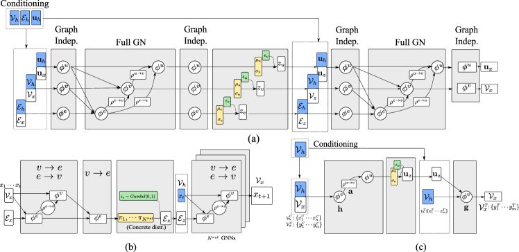
The functions and are implemented by a GN to allow for taking into account in a general manner relational information while inferring over and . In practice a shared, single GN, is used. The parametrization for vertices, edges and global variables are the corresponding states of the GN at the final message passing step. In a similar manner, a GN generator network, , is used for . Since the prior and posterior are factorized over nodes, edges and the global variable of each graph datapoint, the ELBO is split accordingly as
| (8) |
where can be used for controlling disentanglement as in –VAE [15] or the rate-distortion characteristics of the model [1] or for preventing posterior collapse and aiding training through KL-annealing [4, 9]. In a similar manner to VAEs, the approach to representing distributions over graph data with a distribution that factorizes over and allows for defining alternative evidence lower bounds for variational Bayes. Note that the distribution does not need to be factorized along the elements of the latent vector. This allows straight-forward extensions using more flexible distributions [36]. A generative model based on normalizing flows that uses shift-scale transformations [7] has already been proposed in [27] for graph generation. The Relational VAE (RVAE) model proposed can be extended as a hierarchical VAE [42] yielding a model akin to Doubly Stochastic Variational Neural Process (DSNPV) [44], which uses global and node variables. Finally, Neural Processes [10, 11] (NP) and other graph encoder-decoder models [23, 43, 40, 14, 24] are closely related to the proposed model.
3 Related work
GNN Encoder-decoder models
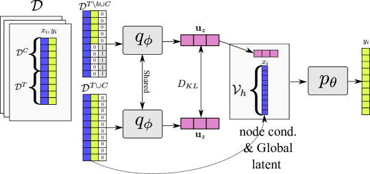
In Neural Relational Inference (NRI) [23] discrete edge latent variables are inferred from node representations and a re-parametrized distribution is used[18, 30]. A coarse representation of the computational graphs of NRI, NPs and the RVAE is shown in Figure 1. In [43] graphs are modeled from global continuous latent variables, which are subsequently used for graph generation through an adjacency matrix. In GraphVAE [40] the global variable together with a graph-structured conditioning variable is used for generation. In Graphite [14] a latent variable for each node is inferred from the encoder, while the edge variables (i.e., symmetric adjacency matrix) is inferred through efficient iterated message passing. Similarly, the VariationalGAE[24] uses a separate latent variable for every node and a graph convolutional encoder. Several of the aforementioned works take advantage of recent advances in low-variance gradient estimates for distributions over latent variables, as in Variational Autoencoders (VAEs) via the reparametrization trick [22, 37]. The overlapping traits of the aforementioned are the treatment of edge, node and global variables. In Table 1 a summary of the relational modeling capabilities of various graph encoder-decoder models is offered. Note that the table highlights only the relevant parts to this work together and several important and influential design choices for graph representation learning were not touched upon. For instance, the graph convolutional models of some of the aforementioned works offer the important advantage of scalability and small computation cost.
In this work, the above mentioned approaches, are generalized and unified in the proposed Relational Variational Autoencoder (RVAE) model. Note that it is not difficult to yield explicit graph connectivity in RVAE as in NRI [23] since the type and existence of a connection can be seen as a categorical variable. See also Figure 1 (b), where a sketch of NRI is offered. Inferring graph connectivity or generating graphs, however, falls out of the scope of this work. In RVAE the focus is generative modeling of graph structured data with an apriori known connectivity, with attributed nodes and edges, which optionally may include a global attribute that influences both entities and relations.
| Latent | Conditioning | ||||||
|---|---|---|---|---|---|---|---|
| Name | Architecture notes | ||||||
| CNP [10] | – | – | – | ✓ | – | ✓ | DeepSet encoder, GN node block |
| AttCNP [20] | – | – | – | ✓ | ✓ | (✓) | Attention encoder/decoder |
| Decoder edge cond. through cross-attention | |||||||
| ConvCNP [13] | – | – | – | ✓ | ✓ | (✓) | SetConv encoder |
| NP [11] | – | – | ✓ | ✓ | – | (✓) | DeepSet encoder |
| GraphVAE [40] | – | – | ✓ | ✓ | ✓ | ✓ | Graph conv. encoder |
| VariationalGAE [24] | ✓ | – | – | – | – | – | Graph convolutions |
| Graphite [14] | ✓ | – | – | ✓ | – | – | Iterative decoder |
| NRI [23] | – | ✓ | – | ✓ | – | – | MP encoder/decoder |
| MPNP [6] | – | – | ✓ | ✓ | ✓ | (✓) | MP encoder/decoder |
| DSVNP [44] | ✓ | – | ✓ | ✓ | – | (✓) | |
| RVAE (this work) | ✓ | ✓ | ✓ | ✓ | ✓ | ✓ | MP encoder/decoder |
Neural processes
In Neural Processes (NP)[10, 11], we consider a set of mappings where . A particular draw of a function , is modeled as where is a high dimensional random vector (e.g. a standard normal) and is a neural network and denotes the parameters of . Given a set of input-output observations from different realizations of (potentially different in number), we want to learn a distribution over . Under the NP approximation, assuming observation noise , the distribution of is defined as
| (9) |
In practice, the input-output observation cases , are split as , where denotes a set of points with observations in and and denotes a set of points where we only observe (i.e., the inputs). This can be cast as a conditional generative model for , where the conditioning is the fully observed context pairs. The ELBO used for optimization is
| (10) |
Note that the above variational objective has an intuitive interpretation, as a reconstruction loss (first part) and a Kullback-Leibler divergence between the approximate posterior distributions predicted when using both and when using only (the context set). In [17] a similar loss function was proposed with the motivation of training VAEs that can be used with arbitrary conditioning masks. By considering the set of observations as nodes in a disconnected graph, (i.e., ) and training while masking the context output nodes , the same objective is retrieved. Therefore, following the nomenclature of [2], we can instantiate a NP from the proposed model, by using arbitrary conditioning as described in [17], a DeepSet [45] as an encoder and only a node-block as a decoder as shown in Figure 1.
The NP framework has been extended to take advantage of special inductive biases, such as the relation of observation and target nodes in Attentive Conditional Neural Processes (AttNP) [20] or the translation equivariance in Convolutional Conditional Neural Processes (ConvCNP) [13]. More recently, relational inductive biases were employed in Message Passing Neural Processes (MPNP) [6]. The aforementioned models, feature a global latent variable which is inferred from the context points and parametrizes the distribution over functions. With the exception of MPMP, the aforementioned works target non-relational data. Nevertheless, MPMPs does not directly implement edge-bound uncertainty or edge-level conditioning, which is the most pronounced difference to RVAE. Similar to this work, in DSNPV [44] a NP that allows for both node and global latent variables was proposed, which in addition, employs a hierarchical VAE [42]. The motivation of DSNPV is to include node-context information, which in the conditional RVAE is also supported by design through . RVAE attempts to merge the complementary strengths of the aforementioned models in representation of uncertainty, with a focus towards modeling graph structured continuous data. Finally, in contrast to Functional Neural Processes [28] we do not deal with inferring a graph of dependencies among latent variables, yet hierarchical RVAE adaptations may also manage such tasks.
Graph Gaussian processes
Sharing the motivation of this work, i.e., taking advantage of relational information and learning joint distributions of graph structured data, in [41] GPs were defined over graphs with undirected binary (positive or negative) edges and applied to semi-supervised learning problems. In [31] the authors applied GPs trained with variational approximations for semi-supervised learning on graphs that contain non-attributed edges. In [26] GP-based approaches are fused with deep learning for learning graph (e.g. network) structured signals.
4 Results
4.1 Wind farm operational data
A real-world industrial application, where relational structure is inherent in the observed data, is found in modeling of operational data of wind turbines positioned in a farm. The wind turbines (nodes) feature static variables, such as their power production characteristics and their position, as well as dynamic variables such as their current operational state. The actual operational state of a turbine is only known up to a certain precision from historical data, (i.e., Supervisory Control and Data Acquisition (SCADA) data), which is usually limited to 10 minute statistics. Due to the stochasticity of the wind excitation, compounded by incomplete information due to coarse measurements, there is uncertainty associated with the actual operational state of a wind turbine. Wind turbines arranged in a wind farm interact through the so-called wakes, which are travelling vortices that affect the power production and vibrations of downstream turbines. The magnitude of wake effects is related to large scale turbulence (which is a global dynamic variable), to wind orientation (which is a global dynamic variable), to upwind turbine nacelle orientation (which is a node dynamic variable), the relative position between the two turbines (an edge static variable), the rotor diameter and the distance between the two turbines. The interaction is one-way directional but can change directionality depending on the wind orientation. The effect of wakes is stochastic due to turbulence. For robust wind power prediction, monitoring, control, and maintenance planning, we want to infer the distribution of operational characteristics of a wind farm conditioned on turbine characteristics and farm layout. Of crucial importance is the inclusion of stochastic variables in the interactions (i.e., edges) of the considered graph. Static graph edges, used as part of the graph conditioning, are constructed by considering the spatial proximity and relative position of pairs of turbines. The goal is to generalize directly to unseen farm configurations while learning directly on real condition monitoring data (zero-shot generalization) but at the same time to yield uncertainty estimates.
Graph machine learning in wind farm modeling
In [33] a GNN was trained on simulated data for wind power prediction. Recently, in [3] GNNs were applied as a surrogate model to more accurate fluid dynamic simulations. With the architectural advancements proposed in this work, we extend the wind farm relational modeling literature by providing a solution for representation of uncertainty in wind turbine interactions. Moreover, we empirically show in real wind farm data that significant accuracy improvements are possible through the incorporation of the proposed relational modeling and variational Bayes approach.
4.2 Real wind farm SCADA dataset
Conditional RVAE models (CRVAE) were trained with with a 80/20 train/test split on a dataset that includes 6 months of 10-minute average SCADA data readings. Since the goal is to compare the fitting capability of the models and not model selection, no validation set was employed. Early stopping with patience of 2500 steps was used (test set evaluation every 500 steps). The larger RVAE models that also yield the best performance had not converged at the 10th epoch. The 20% of turbine data are randomly masked during training. A batch size of 16 was used for all models. In order to make a fair comparison no regularization or KL-annealing was used. A small learning rate of and the Adam optimizer [21] with default parameters was used for all the runs. The final ELBOs for all models are shown in Table 2. A aggregation function and composite aggregation function consisting of a concatenation of , and aggregators were used. Due to the concatenation operation, the composite aggregators result in slightly larger networks. Aligned with recent results on GN performance when using composite aggregation functions [5] we find that networks with the aggregator indeed yield better performance. The motivation, however, for using composite aggregators, is also due to the physics of the problem. By using such aggregators it is easier to discriminate the un-waked part of the farm and the waked turbines. More concretely, turbines at the upstream boundary of the farm have larger power production and this directional effect can easily be masked using the mean aggregation. The CRVAE models are compared to a two-layer MLP-based CVAE trained with the arbitrary conditioning objective [17] of varying sizes, with the largest CVAE model number of parameters corresponding to the number of parameters of the best performing RCVAE. The largest CVAE model was the worst-performing of the evaluated CVAE models.
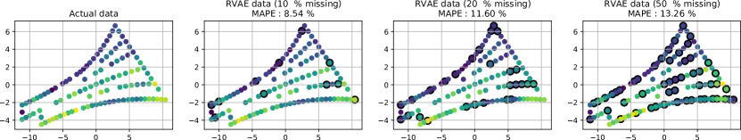
The CVAE model with the smallest size has slightly better performance compared to the RVAE model that performs no message passing on the encoder part, and therefore ignores relational inductive biases when inferring . All but one of the CRVAE models strongly outperform the CVAE models by a large margin which is attributed to the effective use of relational inductive biases. To further support this claim, in the supplemental material (subsection A.2) gradient sensitivities are plotted and it is observed that the imputation results for masked turbines depend on upstream turbines. Qualitative imputation results are shown in Figure 2.
| MP Steps | |||||||
| Model | mlp units | size | enc. | dec. | agg. | # params | ELBO |
| CRVAE | 64 | 32 | 0 | 1 | mean | 184,717 | |
| 64 | 32 | 1 | 1 | mean | 341,517 | ||
| 64 | 32 | 2 | 2 | mean | 498,317 | ||
| 64 | 32 | 2 | 2 | (comp.) | 522,893 | ||
| 64 | 32 | 3 | 3 | (comp.) | 679,693 | ||
| CVAE | 128 | 64 | – | – | – | 77,194 | |
| 256 | 64 | – | – | – | 252,554 | ||
| 384 | 96 | – | – | – | 563,146 | ||
| Case | Range | |
|---|---|---|
Effect of inferring edge latents
The introduction of continuous edge-related latent variables is overlooked in a large part of the literature. Wake effect modeling is an application that may benefit from edge latent variables. We test the effect of edge latent variables by setting while still using . The results of this experiment are shown in Table 3. The inclusion of the KL term with respect to edge latent variables seems to improve the reconstruction error achieved by the model.
4.3 Wind farm simulation dataset
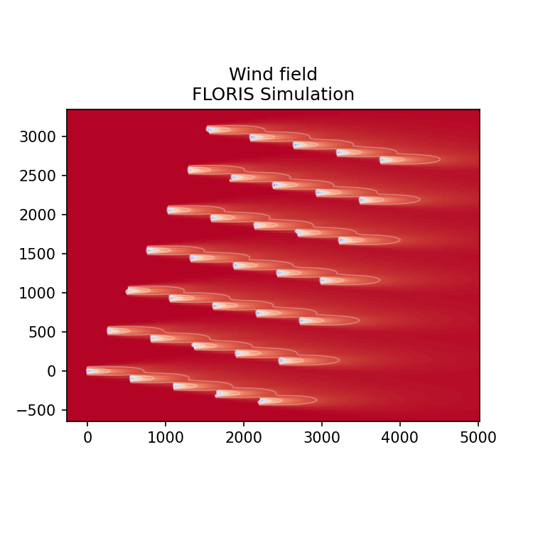
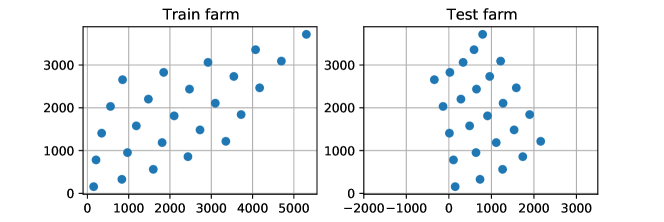
The steady-state wind farm wake simulator FLORIS [32] was used. A dataset of wake effect simulations and preprocessing tools for demonstrating the wind farm modeling approach adopted herein is released as part of this work. In what follows we test the generalization capabilities of a trained RVAE to novel geometric configurations. A single farm configuration is used for training and another one is used for testing. Both farms are simulated with random wind characteristics such as direction and average wind speed. An example output from the simulation can be found in the supplemental material. The train and test farm configurations can also be found in the supplemental material.
Qualitative results
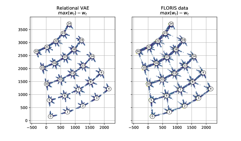
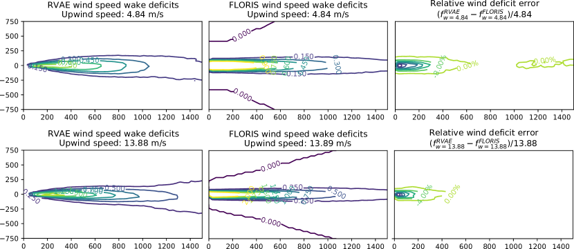
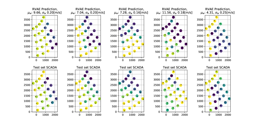
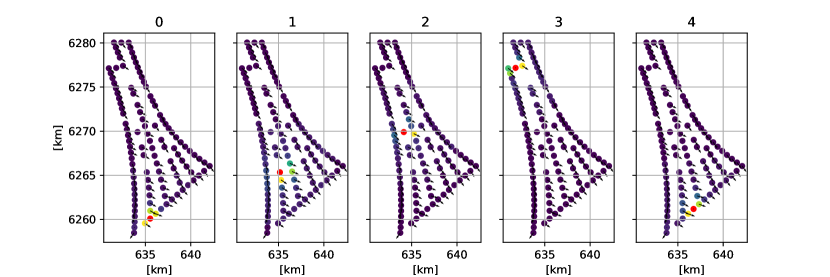
The RVAE model is able to capture the orientation-dependent wake deficit for each turbine separately on the test wind farm as shown in Figure 3. Furthermore, we use a single turbine as a probe and position it on a regular grid while keeping a turbine on a fixed position (0,0). By inspecting the wind speed predicted at the probe turbine, we can map the wake deficit in 2D behind the source turbine. This is shown in Figure 4. The spatial dependence of the wake deficit is also shown as computed from FLORIS and the error in RVAE estimation. For distances larger than the wind deficit is accurately predicted. Note that this result is from a model trained on operational data from a single simulated windfarm. When the turbines are very close () the wakes are not predicted correctly, but this is an expected effect since the RVAE never encounters turbines at these distances. Wake effects estimated with the RVAE are slightly lower than those derived from the simulation as shown in Figure 3. However, the RVAE seems to capture the intricate wind orientation-dependent effects which depend on the farm layout.
4.4 1D regression
In order to further demonstrate the versatility of the RVAE in modeling structured data, and in order to make the connection to NPs [11] clearer, in what follows an RVAE adapted for node data imputation is presented [17]. The dataset consists of sets of points sampled from a zero-mean 1D Gaussian process with a squared exponential kernel. The pairs of input points are used as node features to construct a set of context and target graphs, where corresponds to different GP realizations. Each graph contains a set of edges which encode the relative position of the observation points. The edge features between observations at points are defined as where is a function of the cutoff distance for edge creation. Note that the construction of such edge features endows the model with translation equivariance. In contrast to MPNPs, [6], the edges are the same in the context and target graphs. The loss function used is the same as in subsection B.1. Both and are implemented as GNs. The outputs of the GNs parameterize a Gaussian, i.e.,
| (11) |
The values of are replaced with when fed through the encoder and an additional binary feature for the node, which denotes masking, is appended to the node tuple. The feature is zero for the unmasked nodes and for the masked nodes. The masked input is denoted by . The union of the masked target input with the context dataset is denoted by . Instead of using two different functions for the prior of as in [17], and posterior network and in order to keep the conditional RVAE model closer to the NP formulation, the approximate posterior (i.e., the encoder of the RVAE) is used also for the learned prior. The decoder receives as node conditioning (and optionally edge conditioning) the values and the global latent variable . Each realization of corresponds to a different context set which in turn corresponds to a different sampled . More information about the training setup can be found in the appendix.
The NP is implemented by defining a DeepSet encoder, a global latent variable of the same size as the NP MLP. The same latent variable size for nodes and edges was used for each experiment, which is the same as the core size. All aggregation functions are mean aggregations. Experiments were performed with different number of message passing steps, and inclusion of either the relative observation position as an edge feature or the absolute node position for each feature. The models are tested in un-seen GP realizations and the negative log-likelihood of predictions are reported in Table 4. The RVAE models compute edge, node and global variables. The test datasets contain points with and ranges in order to test the generalization capability of the proposed model in translation. Since the edge-blocks only ever receive translation equivariant inputs from the dataset, the RVAE models generalize well in the range. This is presented only as an example of how special equivariant inductive biases may be implemented in RVAE. It is observed that the full RVAE model does not perform well when only the node features are available. As with NPs, it was empirically found that models yield better results with more training.
| Model | size | Only cond. on nodes | Cond. on edges and nodes | ||
| (mlp//MP Steps) | |||||
| CRVAE | 64/64/0 | ||||
| 64/64/1 | |||||
| 64/64/2 | – | – | |||
| NP | 64/64/NA | NA | NA | ||
| 128/128/NA | NA | NA | |||
Conclusions and broader impact
This work introduces an attributed graph approach to the probabilistic modeling of relations within entities and their properties. The approach is verified and validated on wake effect simulations and actual data from wind turbines placed within a wind farm; a characteristic example that may be modeled as a graph. We also find some connections to the NP literature which we demonstrate by adapting the proposed method to perform a typical NP benchmark which is 1D regression for GP data.
We introduce a method for data-driven wake effect modeling for wind farms that accounts for uncertainty. The proposed method fuses physical intuition, flexible function approximation through GNs, and variational Bayes through re-parametrized gradients. Better and more computationally efficient wake effect modeling can lead to improvements in terms of accuracy and computational efficiency in analysis for wind farm siting [29] farm layout optimization [25], wind farm control optimization [16] and ultimately power production improvements, as well as more robust to uncertainties maintenance planning. Ultimately, the aforementioned lead to wind energy being a more attractive clean energy solution.
Graph data are naturally used to model social, transportation and communication networks. Possible negative implications of any graph ML work relate to possible malicious uses of analysis in such networks, such as de-anonymization in social networks [19], and vulnerability exploitation on transportation networks.
Acknowledgments and Disclosure of Funding
The authors would like to gratefully acknowledge the support of the European Research Council via the ERC Starting Grant WINDMIL (ERC-2015- StG #679843) on the topic of Smart Monitoring, Inspection and Life-Cycle Assessment of Wind Turbines.
References
- [1] A. Alemi, B. Poole, I. Fischer, J. Dillon, R. A. Saurous, and K. Murphy. Fixing a broken ELBO. In J. Dy and A. Krause, editors, Proceedings of the 35th International Conference on Machine Learning, volume 80 of Proceedings of Machine Learning Research, pages 159–168. PMLR, 10–15 Jul 2018.
- [2] P. W. Battaglia, J. B. Hamrick, V. Bapst, A. Sanchez-Gonzalez, V. Zambaldi, M. Malinowski, A. Tacchetti, D. Raposo, A. Santoro, R. Faulkner, et al. Relational inductive biases, deep learning, and graph networks. arXiv preprint arXiv:1806.01261, 2018.
- [3] J. Bleeg. A graph neural network surrogate model for the prediction of turbine interaction loss. In Journal of Physics: Conference Series, volume 1618, page 062054. IOP Publishing, 2020.
- [4] S. R. Bowman, L. Vilnis, O. Vinyals, A. M. Dai, R. Jozefowicz, and S. Bengio. Generating sentences from a continuous space. arXiv preprint arXiv:1511.06349, 2015.
- [5] G. Corso, L. Cavalleri, D. Beaini, P. Liò, and P. Veličković. Principal neighbourhood aggregation for graph nets. arXiv preprint arXiv:2004.05718, 2020.
- [6] B. Day, C. Cangea, A. R. Jamasb, and P. Liò. Message passing neural processes. arXiv preprint arXiv:2009.13895, 2020.
- [7] L. Dinh, J. Sohl-Dickstein, and S. Bengio. Density estimation using real nvp. arXiv preprint arXiv:1605.08803, 2016.
- [8] Y. Dubois, J. Gordon, and A. Y. Foong. Neural process family. http://yanndubs.github.io/Neural-Process-Family/, September 2020.
- [9] H. Fu, C. Li, X. Liu, J. Gao, A. Celikyilmaz, and L. Carin. Cyclical annealing schedule: A simple approach to mitigating kl vanishing. arXiv preprint arXiv:1903.10145, 2019.
- [10] M. Garnelo, D. Rosenbaum, C. Maddison, T. Ramalho, D. Saxton, M. Shanahan, Y. W. Teh, D. Rezende, and S. A. Eslami. Conditional neural processes. In International Conference on Machine Learning, pages 1704–1713. PMLR, 2018.
- [11] M. Garnelo, J. Schwarz, D. Rosenbaum, F. Viola, D. J. Rezende, S. Eslami, and Y. W. Teh. Neural processes. arXiv preprint arXiv:1807.01622, 2018.
- [12] J. Gilmer, S. S. Schoenholz, P. F. Riley, O. Vinyals, and G. E. Dahl. Neural message passing for quantum chemistry. In International Conference on Machine Learning, pages 1263–1272. PMLR, 2017.
- [13] J. Gordon, W. P. Bruinsma, A. Y. Foong, J. Requeima, Y. Dubois, and R. E. Turner. Convolutional conditional neural processes. arXiv preprint arXiv:1910.13556, 2019.
- [14] A. Grover, A. Zweig, and S. Ermon. Graphite: Iterative generative modeling of graphs. In International conference on machine learning, pages 2434–2444. PMLR, 2019.
- [15] I. Higgins, L. Matthey, A. Pal, C. Burgess, X. Glorot, M. Botvinick, S. Mohamed, and A. Lerchner. -vae: Learning basic visual concepts with a constrained variational framework. 2016.
- [16] M. F. Howland, S. K. Lele, and J. O. Dabiri. Wind farm power optimization through wake steering. Proceedings of the National Academy of Sciences, 116(29):14495–14500, 2019.
- [17] O. Ivanov, M. Figurnov, and D. Vetrov. Variational autoencoder with arbitrary conditioning. arXiv preprint arXiv:1806.02382, 2018.
- [18] E. Jang, S. Gu, and B. Poole. Categorical reparameterization with gumbel-softmax. arXiv preprint arXiv:1611.01144, 2016.
- [19] S. Ji, P. Mittal, and R. Beyah. Graph data anonymization, de-anonymization attacks, and de-anonymizability quantification: A survey. IEEE Communications Surveys & Tutorials, 19(2):1305–1326, 2016.
- [20] H. Kim, A. Mnih, J. Schwarz, M. Garnelo, A. Eslami, D. Rosenbaum, O. Vinyals, and Y. W. Teh. Attentive neural processes. arXiv preprint arXiv:1901.05761, 2019.
- [21] D. P. Kingma and J. Ba. Adam: A method for stochastic optimization. arXiv preprint arXiv:1412.6980, 2014.
- [22] D. P. Kingma and M. Welling. Auto-encoding bariational bayes. arXiv preprint arXiv:1312.6114, 2013.
- [23] T. Kipf, E. Fetaya, K.-C. Wang, M. Welling, and R. Zemel. Neural relational inference for interacting systems. In International Conference on Machine Learning, pages 2688–2697. PMLR, 2018.
- [24] T. N. Kipf and M. Welling. Variational graph auto-encoders. arXiv preprint arXiv:1611.07308, 2016.
- [25] N. Kirchner Bossi and F. Porté-Agel. Multi-objective wind farm layout optimization with unconstrained area shape. In Wind Energy Science Conference 2019 (WESC 2019), number POST_TALK, 2019.
- [26] N. Li, W. Li, J. Sun, Y. Gao, Y. Jiang, and S.-T. Xia. Stochastic deep gaussian processes over graphs. In H. Larochelle, M. Ranzato, R. Hadsell, M. F. Balcan, and H. Lin, editors, Advances in Neural Information Processing Systems, volume 33, pages 5875–5886. Curran Associates, Inc., 2020.
- [27] J. Liu, A. Kumar, J. Ba, J. Kiros, and K. Swersky. Graph normalizing flows. arXiv preprint arXiv:1905.13177, 2019.
- [28] C. Louizos, X. Shi, K. Schutte, and M. Welling. The functional neural process. arXiv preprint arXiv:1906.08324, 2019.
- [29] J. Lundquist, K. DuVivier, D. Kaffine, and J. Tomaszewski. Costs and consequences of wind turbine wake effects arising from uncoordinated wind energy development. Nature Energy, 4(1):26–34, 2019.
- [30] C. J. Maddison, A. Mnih, and Y. W. Teh. The concrete distribution: A continuous relaxation of discrete random variables. arXiv preprint arXiv:1611.00712, 2016.
- [31] Y. C. Ng, N. Colombo, and R. Silva. Bayesian semi-supervised learning with graph gaussian processes. arXiv preprint arXiv:1809.04379, 2018.
- [32] NREL. FLORIS. Version 2.2.0, 2020.
- [33] J. Park and J. Park. Physics-induced graph neural network: An application to wind-farm power estimation. Energy, 187:115883, 2019.
- [34] T. Pfaff, M. Fortunato, A. Sanchez-Gonzalez, and P. W. Battaglia. Learning mesh-based simulation with graph networks. arXiv preprint arXiv:2010.03409, 2020.
- [35] B. R. Resor. Definition of a 5mw/61.5 m wind turbine blade reference model. Albuquerque, New Mexico, USA, Sandia National Laboratories, SAND2013-2569, 2013, 2013.
- [36] D. Rezende and S. Mohamed. Variational inference with normalizing flows. In F. Bach and D. Blei, editors, Proceedings of the 32nd International Conference on Machine Learning, volume 37 of Proceedings of Machine Learning Research, pages 1530–1538, Lille, France, 07–09 Jul 2015. PMLR.
- [37] D. J. Rezende, S. Mohamed, and D. Wierstra. Stochastic backpropagation and approximate inference in deep generative models. In International conference on machine learning, pages 1278–1286. PMLR, 2014.
- [38] A. Sanchez-Gonzalez, J. Godwin, T. Pfaff, R. Ying, J. Leskovec, and P. Battaglia. Learning to simulate complex physics with graph networks. In H. D. III and A. Singh, editors, Proceedings of the 37th International Conference on Machine Learning, volume 119 of Proceedings of Machine Learning Research, pages 8459–8468. PMLR, 13–18 Jul 2020.
- [39] V. G. Satorras, E. Hoogeboom, and M. Welling. E (n) equivariant graph neural networks. arXiv preprint arXiv:2102.09844, 2021.
- [40] M. Simonovsky and N. Komodakis. Graphvae: Towards generation of small graphs using variational autoencoders. In International Conference on Artificial Neural Networks, pages 412–422. Springer, 2018.
- [41] W. C. V. Sindhwani, Z. Ghahramani, and S. S. Keerthi. Relational learning with gaussian processes. In Advances in Neural Information Processing Systems 19: Proceedings of the 2006 Conference, volume 19, page 289. MIT Press, 2007.
- [42] C. K. Sønderby, T. Raiko, L. Maaløe, S. K. Sønderby, and O. Winther. Ladder variational autoencoders. arXiv preprint arXiv:1602.02282, 2016.
- [43] M. Tavakoli and P. Baldi. Continuous representation of molecules using graph variational autoencoder. arXiv preprint arXiv:2004.08152, 2020.
- [44] Q. Wang and H. Van Hoof. Doubly stochastic variational inference for neural processes with hierarchical latent variables. In International Conference on Machine Learning, pages 10018–10028. PMLR, 2020.
- [45] M. Zaheer, S. Kottur, S. Ravanbakhsh, B. Poczos, R. Salakhutdinov, and A. Smola. Deep sets. arXiv preprint arXiv:1703.06114, 2017.
- [46] V. Zambaldi, D. Raposo, A. Santoro, V. Bapst, Y. Li, I. Babuschkin, K. Tuyls, D. Reichert, T. Lillicrap, E. Lockhart, et al. Relational deep reinforcement learning. arXiv preprint arXiv:1806.01830, 2018.
Appendix A Appendix
A.1 RVAE on wind farm monitoring data
The steady-state wind farm wake simulator FLORIS was used [32] for the simulated dataset. An example output of a simulation from FLORIS is shown in Figure 5.
Additional details on farm graph construction
A graph is constructed where turbines are the vertices and directed edges are created between the turbines by truncating an all-to-all graph to a cut-off distance of where is the turbine rotor diameter. The 5MW NREL prototype turbine was used for the simulations [35] which has a diameter . In order to test the generalization capabilities of the model, and most importantly the ability to implicitly learn how to use the relative position of the turbines and the nacelle wind orientation and power production of up-wind turbines, the model is tested on a different farm configuration than the one it is trained on. It is noted that the wake simulator used is not stochastic. The yaw directions of the turbines were randomly perturbed with around the global wind orientation in order to introduce some stochasticity. The training dataset consists of farm SCADA readings for the whole farm. Both farms are simulated with the same randomly sampled mean wind and wind orientation global conditions (). Due to the different arrangement of the turbines in the two farms and their wake interactions the wind speed and power production of the two farms is very different. The farm configurations are shown in Figure 6.
Treatment of angles
As shown in Figure 7, the angle of the directional vector defined by the sender turbine to the receiver turbine , and distance are used as an edge feature. In real farm monitoring data, the turbine yaw is adjusted by a per-turbine controller during operation according to the wind conditions and may be different for each turbine. The yaw angle with respect to north is used as a node feature together with mean and standard deviation of hub-height wind speed when available, and power production.
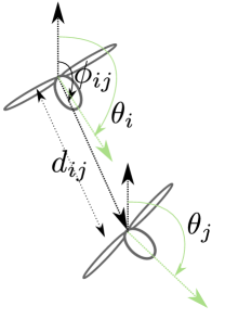
Since the relative angle of the line defined between the turbines and the yaw angles is important, and not the absolute angles, a simple data augmentation procedure is performed during training where both yaw angle and the farm positions are randomly rotated with the same angle. A more general solution to the problem of learning networks that respect transformations to such symmetries would be to use GNs which are equivariant by design as proposed in [39] but this is left for future work.
Further qualitative results on the simulated farm dataset
In Figure 8 some RVAE predictions and actual data from the simulated farm test set are shown. Note that the configuration of the test farm is unseen and no training is performed. The RVAE seems to capture the wake-associated wind deficits of the farm in all but one case (second from the right).
A.2 Anholt farm dataset
Post-hoc model interpretation with gradient sensitivities
In order to identify which nodes are important for the imputed values for a particular turbine, a simple gradient sensitivity technique was employed. For a particular node prediction , and a RVAE model with recognition model and generator , we have where is the graph that contains the masked target nodes and all the edges between context and target nodes. Since the model is end-to-end differentiable, one can straightforwardly compute an absolute gradient sensitivity as
| (12) |
An instance of such maps is visualized for a farm state snapshot and for a representative set of turbines in Figure 9. Wind orientation is inferred from turbine nacelle orientation and it is visualized as arrows centered at each turbine and pointing towards the incoming wind. The upwind turbines seem to contribute more to the imputation value of the masked turbines. This is aligned with the physics of the problem and in particular with the directionality of the wake effects which is always from upstream to downstream turbines. The values of the turbines in the undisturbed boundaries of the farm as in plots indexed 0 and 4 rely on non-upstream neighbors for imputation. This also is expected, as there is no up-wind information for the imputation so the network needs to rely on any neighbors to impute the wind velocity values.
Appendix B Supplemental material for the NP section
Additional details on the training setup
All experiments were performed using the Adam optimizer [21] with a learning rate of and default parameters. All RVAE models were trained for steps and NP models up to steps with batches of size 16. Each batch contains a random number of context and target points which varies between 3 and 50. All GN functions involved are feed-forward 3-layer Multi-Layer Perceptron (MLPs) with rectified linear unit non-linearities and no activation in the last layer. The GN block used is encode-process-decode architecture as in [2] with residual connections. The encoder and decoder contain layers that do not perform message passing but only cast the inputs to a predefined dimension (Graph Independent layers).
Qualitative results on 1D regression meta-learning
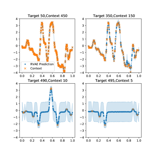
In Figure 11 qualitative results for the behavior of the RVAE for varying numbers of context points are shown. In the absence of context points, the model tends to predict the mean which is zero for the training dataset. Upon review, a notebook will be released demonstrating the implementation of the method.
B.1 Implementation of NP as a VAE with arbitrary conditioning
In order to make the exposition of the main text clearer in what follows the ELBO objective for a RVAE model with arbitrary conditioning and a DeepSet encoder is detailed. In the NP implementation a set of context and target points are encoded through to a global Gaussian latent variable . Now consider the NP problem as a missing data imputation problem, where the context points, are observed sets of points from a function, and the target points are points coming from the same function where we only have their coordinate () and we seek to evaluate the values. The NP approach to this problem is to separately encode and to a Gaussian latent space using a DeepSet encoder, use the known as conditioning, and compute using and (and optionally a deterministic introduced in [20]). The loss function for NPs given in subsection B.1 can be cast as an arbitrary conditioning objective as in [17].
The VAE-AC[17] approach to an imputation problem such as this one, is to augment the dataset with an additional variable which signifies whether points are observed or unobserved. The term of the ELBO objective drives the latent representation of the recognition network to be similar when observing and . A network with parameters is jointly trained to yield . The arbitrary conditioning ELBO objective in that case reads,
| (13) |
The VAE-AC approach is particularly convenient for the RVAE which contains message passing layers, since no special message passing needs to be performed between observed and unobserved points. In Figure 10 a more detailed computational diagram is shown.