Charged and Neutral $\bar{B}_{u,d,s}\to\gamma$ Form Factors from
Light Cone Sum Rules at NLO

Abstract

We present the first analytic ${\cal O}(\alpha_{s})$-computation at twist-$1$,$2$ of the $\bar{B}_{u,d,s}\to\gamma$ form factors within the framework of sum rules on the light-cone. These form factors describe the charged decay $\bar{B}_{u}\to\gamma\ell^{-}\bar{\nu}$, contribute to the flavour changing neutral currents $\bar{B}_{d,s}\to\gamma\ell^{+}\ell^{-}$ and serve as inputs to more complicated processes. We provide a fit in terms of a $z$-expansion with correlation matrix and extrapolate the form factors to the kinematic endpoint by using the $g_{BB^{*}\gamma}$ couplings as a constraint. Analytic results are available in terms of multiple polylogarithms as ancillary files. We give binned predictions for the $\bar{B}_{u}\to\gamma\ell^{-}\bar{\nu}$ branching ratio along with the associated correlation matrix. By comparing with three SCET-computations we extract the inverse moment $B$-meson distribution amplitude parameter $\lambda_{B}=360(110)\textrm{\small MeV}$. The uncertainty thereof could be improved by a more dedicated analysis. In passing, we extend the photon distribution amplitude to include quark mass corrections with a prescription for the magnetic vacuum susceptibility, $\chi_{q}$, compatible with the twist-expansion. The values $\chi_{q}=3.21(15)\textrm{\small GeV}^{-2}$ and $\chi_{s}=3.79(17)\textrm{\small GeV}^{-2}$ are obtained.

1 Introduction

In this work we provide the (photon) on-shell form factors contributing to semileptonic $\bar{B}_{u}\to\gamma\ell^{-}\bar{\nu}$ and flavour changing neutral decay (FCNC) $\bar{B}_{d,s}\to\gamma\ell^{+}\ell^{-}$ with the method of light-cone sum rules (LCSR). This is the first complete next-to leading order (NLO) computation in $\alpha_{s}$ including twist-$1$,$2$ and leading order (LO) twist-$3$ and partial twist-$4$. The dynamics, contrary to naive expectation, are more involved than for $\bar{B}\to V(\rho,\omega,K^{*},\phi)$BB98b ; BZ04b . This comes as the point-like photon, of leading twist-$1$, has no counterpart for the mesons and yet the photon is to be described by a photon distribution amplitude (DA) (analogous to the vector meson case and cf. Tab. 11 for a dictionary). The photon DA can be interpreted as $\rho_{0},\omega_{0},\phi$-$\gamma$ conversion and is normalised by the QCD magnetic vacuum susceptibility $\chi$, for which we propose a prescription to include quark mass effects in Sec. 4.2.1. The twist-$1$ part leading in the heavy quark scaling $F^{\bar{B}\to\gamma}\propto m_{b}^{-1/2}$, differing from $F^{\bar{B}\to V}\propto m_{b}^{-3/2}$, which we discuss in the hadronic picture in the large-$N_{c}$ limit using a dispersion in Sec. 2.3.

In the literature the charged $\bar{B}_{u}\to\gamma$ form factors have been considered in LCSR at leading order (LO) in $\alpha_{s}$ in Khodjamirian:1995uc ; Ali:1995uy ; Eilam:1995zv and a partial (no twist-$1$) NLO contribution in Ball:2003fq . The decay has received considerable attention in QCD-factorisation and soft-collinear effective theory (SCET), in part, as a toy model for factorisation and for its prospect to extract parameters of the $B$-meson’s distribution amplitude parameters Korchemsky:1999qb ; Lunghi:2002ju ; DescotesGenon:2002mw ; Bosch:2003fc ; Beneke:2011nf ; Braun:2012kp ; Wang:2016qii ; Beneke:2018wjp ; Wang:2018wfj ; Galda:2020epp ; Shen:2020hsp . In Sec. 5.4 we extract the $B$-meson DA parameters $\lambda_{B}$ by comparing to a SCET evaluation in three representative models. SCET-investigations include Korchemsky:1999qb ; Lunghi:2002ju ; DescotesGenon:2002mw ; Bosch:2003fc at leading power and Beneke:2011nf at next-to-leading log and partial sub-leading powers. Subleading powers, (partially) corresponding to the photon DA, were accounted for by dispersion techniques Braun:2012kp ; Wang:2016qii ; Beneke:2018wjp . Other approaches include perturbative QCD Shen:2018abs and a hybrid approach of QCD factorisation and LCSR Wang:2018wfj to which we compare in Sec. 4.3. A first lattice form factor evaluation has been reported for $D_{(s)},K,\pi\to\gamma$ in Desiderio:2020oej and further evaluations of $D_{s}(K)\to\gamma$ are in progress Kane:2019jtj .

The neutral $\bar{B}_{d,s}\to\gamma$ form factors describe flavour changing neutral currents which are generic probes for physics beyond the Standard Model. The activity in this particular corner has been revived, since it has been pointed out Dettori:2016zff that, in a certain kinematic region, $\bar{B}_{s}\to\gamma\mu^{+}\mu^{-}$ may be extracted from the very same dataset as $\bar{B}_{s}\to\mu^{+}\mu^{-}$ at LHC experiments Aaij:2017vad ; Aaboud:2018mst ; CMS:2019qnb (cf. also Aditya:2012im ). This triggered a number of phenomenological investigations GRZ17 ; Kozachuk:2017mdk ; Beneke:2020fot ; Carvunis:2021jga . Previously these form factors had been considered, in LCSR at LO Aliev:1996ud , in Kruger:2002gf using aspects of heavy quark symmetry (with input from Beyer:2001zn ), quark model computations MN04 ; Kozachuk:2017mdk and more recently in SCET Beneke:2020fot . In addition, in this decay, the dipole operator $m_{b}\bar{q}_{L}\sigma\!\cdot\!Fb$ necessitates photon off-shell form factors. These have been investigated for the first time, at LO with QCD sum rules Albrecht:2019zul , utilising the on-shell form factors of this paper as an input.

The paper is organised as follows. In Sec. 2 the form factors are defined and their heavy quark scaling is discussed in a hadronic picture. In Sec. 3 the correlation functions entering the computation, Ward identities and contact terms (CTs ) are discussed extensively. The evaluation at LO and NLO for the perturbative and soft parts is documented in Sec. 4. The numerics Sec. 5 contains our main practical results in terms of fits, plots, the extraction of the inverse moment of the $B$-meson DA and the binned prediction for the $\bar{B}_{u}\to\gamma\ell^{-}\bar{\nu}$ rate in Secs. 5.1, 5.2, 5.3 and 5.4 respectively. The paper ends with summary and conclusions in Sec. 6. Appendices include conventions and comments on form factor definitions (Apps. A), gauge invariance of the amplitude (App. B), coordinate space equation of motion (including their non-trivial renormalisation) (App. C), a compendium of photon DAs (App. D), results of correlation functions (App. E) and discontinuities of multiple-polylogarithms in (App. F).

2 Generalities on the $\bar{B}\to\gamma$ Form Factors

The section provides the method-independent information on the $B\to\gamma$ form factors (FFs), such as the definition and the heavy quark scaling.

2.1 Definition of the Form Factors

Amongst the dimension six operators of the $b\to q$ effective Hamiltonian there are the standard vector and tensor operators. Note that the scalar operator vanishes by parity conservation of QCD and the pseudoscalar one only contributes for an off-shell photon (cf. reference Albrecht:2019zul for a complete discussion). We consider, in addition, an operator which is redundant by the equation of motion (EOM) but that will prove useful as a check and is of interest per se Hambrock:2013zya ; BSZ15 . In complete generality, with conventions as in GRZ17 ; Albrecht:2019zul , extended to include the charged case, we define the FFs

$$\langle\gamma(k,\epsilon)|O^{V}_{\mu}|\bar{B}_{q}(p_{B})\rangle \;=\; s_{e}(P^{\perp}_{\mu}\,V_{\perp}(q^{2}) \;-\; P^{\parallel}_{\mu}\,(V_{\parallel}(q^{2})+Q_{\bar{B}_{q}}f^{(pt)}_{B_{q}})-P^{\textrm{Low}}_{\mu}Q_{\bar{B}_{q}}f^{(pt)}_{B_{q}})~{},$$

$$\langle\gamma(k,\epsilon)|O^{T}_{\mu}|\bar{B}_{q}(p_{B})\rangle \;=\; s_{e}(P^{\perp}_{\mu}\,T_{\perp}(q^{2}) \;-\; P^{\parallel}_{\mu}\,T_{\parallel}(q^{2}))~{},$$ (1)

$$\langle\gamma(k,\epsilon)|O^{\cal D}_{\mu}|\bar{B}_{q}(p_{B})\rangle \;=\; s_{e}(P_{\perp}^{\mu}\,{\cal D}_{\perp}(q^{2}) \;-\; P_{\parallel}^{\mu}\,({\cal D}_{\parallel}(q^{2})+\hat{m}_{-}\,Q_{\bar{B}_{q}}f^{(pt)}_{B_{q}})-P^{\textrm{Low}}_{\mu}\hat{m}_{-}\,Q_{\bar{B}_{q}}f^{(pt)}_{B_{q}})\;,$$

where $\hat{m}_{\pm}\equiv m_{\pm}/m_{B_{q}}$, $m_{\pm}\equiv(m_{b}\pm m_{q})$ and $Q_{\bar{B}_{q}}=Q_{b}-Q_{q}$ is the charge of the $\bar{B}_{q}$-meson. Comparison with literature-conventions are deferred to the next section. Hereafter,

$$f^{(pt)}_{B_{q}}=\frac{m_{B_{q}}f_{B_{q}}}{k\cdot p_{B}}=\frac{2f_{B_{q}}/m_{B_{q}}}{1-q^{2}/m_{B_{q}}^{2}}$$ (2)

denotes the point-like (or scalar QED) contribution, proportional to the decay constant, and consists of the infrared (IR) sensitive Low-term, which captures the gauge variance of the matrix element on the LHS (for charged $\bar{B}_{q}$) and assures that the FFs themselves are gauge invariant (cf. Sec. 3.2 and App. B.1). The gauge variance of the matrix element is cancelled in the full $\bar{B}_{u}\to\gamma\ell^{-}\bar{\nu}$ amplitude when the photon-emission from the lepton is added cf. App. B.2. The same terms appears in $P_{\parallel}^{\mu}$-structure whose subtraction from the FF was stressed in Carrasco:2015xwa ; Desiderio:2020oej cf. Sec. 2.2. Furthermore, $s_{e}$ is the sign-convention of the covariant derivative (cf. App. A), $p_{B}=q+k$, on-shell momenta $p_{B}^{2}=m_{B}^{2}$, $k^{2}=0$, $f_{B_{q}}$ the decay constant

$$\langle 0|\bar{q}\gamma^{\mu}\gamma_{5}b|\bar{B}_{q}(p_{B})\rangle=ip_{B}^{\mu}f_{B_{q}}\;,$$ (3)

local operators (describing the $b\to q$ transition)

$$O^{V}_{\mu}\equiv-\frac{1}{e}m_{B_{q}}\bar{q}\gamma_{\mu}(1-\gamma_{5})b\;,\quad O^{T}_{\mu}\equiv\frac{1}{e}\bar{q}iq^{\nu}\sigma_{\mu\nu}(1+\gamma_{5})b\;,\quad O^{\cal D}_{\mu}\equiv\frac{1}{e}\bar{q}(i\!\overset{\leftrightarrow}{D})_{\mu}(1+\gamma_{5})b\;,$$ (4)

and Lorentz structures ($\varepsilon_{0123}=1$ convention, $e=\sqrt{4\pi\alpha}>0$ and $P^{\perp,\parallel,\textrm{Low}}_{\mu}\equiv\epsilon^{*\rho}P^{\perp,\parallel,\textrm{Low}}_{\mu\rho}$)

$$P^{\perp}_{\mu\rho}\equiv\varepsilon_{\mu\rho\beta\gamma}(p_{B})^{\beta}k^{\gamma}\;,\quad P^{\parallel}_{\mu\rho}\equiv i\,(p_{B}\cdot k\,g_{\mu\rho}-k_{\mu}\,(p_{B})_{\rho})\;,\quad P^{\textrm{Low}}_{\mu\rho}\equiv i(p_{B})_{\mu}(p_{B})_{\rho}\;.$$ (5)

The Lorentz structures are transverse, $q\cdot P^{\perp,\parallel}=0$, due to the $\lambda=\pm 1$-helicity of the photon. As usual the Lorenz gauge, $k\cdot\epsilon(\lambda,k)=0$, is assumed and $\epsilon\to\epsilon+k$ is the residual gauge invariance encoded as $P^{\perp,\parallel}|_{\epsilon\to k}=0$. By writing the Lorentz decomposition of $\langle\gamma(k,\epsilon)|\,\bar{q}i\sigma^{\mu\nu}(1\!+\!\gamma_{5})b\,|\bar{B}_{q}(p_{B})\rangle$ and using the algebraic relation (A.2) the FF relation

$$T_{\perp}^{B\to\gamma}(0)=T_{\parallel}^{B\to\gamma}(0)\;,$$ (6)

can be shown to hold, in complete analogy to the $B\to V$ FFs, $T_{1}^{B\to V}(0)=T_{2}^{B\to V}(0)$.

A short comment on the $\perp,\parallel$ subscripts. Interpreting the FF as a $\bar{B}\to 1^{-(+)}\gamma$ transition, $\perp(\parallel)$ correspond to perpendicular (parallel) $3$-dimensional polarisation vectors of the photon and the $1^{-(+)}$ state (as can be seen from (5)). In the $B\to V\ell\ell$ literature, e.g. Kou:2018nap , the $\perp,\parallel$ combinations are known as the transversity amplitudes and are useful because of definite CP-parities.

2.1.1 Form Factor Conventions in the Literature

We wish to explain why we have adopted a different notation w.r.t. to some of the literature. There are three reasons: firstly, in the off-shell case there are $7$ FFs Albrecht:2019zul for which the $F_{A,V}$ notation becomes inefficient. Second, the subtraction of the point-like term in the charged case following Carrasco:2015xwa ; Desiderio:2020oej (cf. Fig. 9 for comparison). Third, in GRZ17 the sign of the FFs was chosen such that the $\bar{B}_{d,s}\to\gamma$ FFs are positive, and since the spectator quark is dominant this implies that the $\bar{B}_{u}\to\gamma$ FFs are negative. The latter explains the sign difference

$$V^{\bar{B}_{u}\to\gamma}_{\perp}=-F^{\bar{B}_{u}\to\gamma}_{V}\;,\quad V^{\bar{B}_{u}\to\gamma}_{\parallel}+Q_{\bar{B}_{u}}f^{(pt)}_{\bar{B}_{u}}=-F^{\bar{B}_{u}\to\gamma}_{A}\;,$$ (7)

w.r.t. to the SCET-literature with focus on the charged transition. Compared with Desiderio:2020oej we find

$$V^{D_{s}\to\gamma}_{\perp}=-F^{D_{s}\to\gamma}_{V}\;,\quad V^{D_{s}\to\gamma}_{\parallel}=-F^{D_{s}\to\gamma}_{A}\;,$$ (8)

assuming their translation to the SCET-literature. Essentially these are the same conventions as in (7) with the point-like part separated, which hopefully will become the new standard. When comparing with MN04 ; Kozachuk:2017mdk we believe the following map should be used

$$V^{\bar{B}_{d,s}\to\gamma}_{\perp,\parallel}=F^{\bar{B}_{d,s}\to\gamma}_{V,A}\;,\quad T^{\bar{B}_{d,s}\to\gamma}_{\perp,\parallel}=FT^{\bar{B}_{d,s}\to\gamma}_{V,A}\;.$$ (9)

Note that in comparing analytic results one needs to keep in mind that the signs of $\chi$ and $s_{e}$ (and $s_{g}$) are author-dependent as well.

2.2 $B\to\gamma$ Form Factor in the context of QED-corrections to leptonic decays

Since the $B\to\gamma$ FFs are the real emission corrections to the leptonic decay $B^{+}\to\ell^{+}\nu$ or part of the FCNC $B_{d,s}\to\ell^{+}\ell^{-}$, we consider it worthwhile to clarify a few aspects with regards to QED-corrections to leptonic decays: the point-like term indicated in (2.1), the absence $\ln m_{\ell}$-terms, the importance of the kinematic endpoint and extrapolations. The arguments below go beyond $B$-physics since infrared effects are rather universal.

In the charged case the photon couples to the charged $B$-meson, there is a point-like or monopole contribution which can be identified by matching the axial current $A_{5\mu}=\bar{q}\gamma_{\mu}\gamma_{5}b$ to a meson current $A_{5\mu}\to-f_{B}D_{\mu}\bar{B}^{\dagger}$, with $\langle 0|B^{\dagger}(x)|\bar{B}\rangle=e^{-ip_{B}\cdot x}$ such that (3) holds. One then easily finds

$$\langle\gamma|A_{5\mu}|{\bar{B}}\rangle=f_{B}(-ies_{e}Q_{\bar{B}})\epsilon^{*\rho}\left(g_{\rho\mu}+\frac{(2p_{B}-k)_{\rho}q_{\mu}}{2k\cdot p_{B}-k^{2}}\right)\;,$$ (10)

where the metric term comes from the photon field in the covariant derivative. Upon using $k^{2}=0$ and $\epsilon^{*}\cdot k=0$ one recovers the form in (2.1).

It seems worthwhile to point out that leptonic decays are free from hard-collinear logs of the form ${\cal O}(\alpha\ln m_{\ell})$, as these have been shown to vanish from structure-dependent corrections by gauge invariance (cf. section 3.4 in Isidori:2020acz ). Thus they can only arise from the point-like contribution which is itself free from $\ln m_{\ell}$-terms. This can be seen as follows. In the real emission the collinear terms would arise from the Low-term which is proportional to the helicity-suppressed LO term and therefore the logs are of the form $m^{2}_{\ell}\ln m_{\ell}$ at worst. Finally, since real and virtual point-like contributions cancel each other in the photon-inclusive rate the virtual corrections must be free from such terms altogether. This completes the argument.

In the actual measurement of $B^{+}\to\ell^{+}\nu$ the undetected photon is soft and $q^{2}$ is very close to the kinematic endpoint, which is beyond the limit of the direct LCSR computation. This underlines the importance of the extrapolation as discussed in Sec. 5.1.2 (based on the $g_{BB*\gamma}$ couplings Pullin:2021ebn ). A more direct sum rule analysis or the lattice approaches mentioned earlier are of course an alternative thereto. We will report on the impact of $B_{s}\to\gamma\ell^{+}\ell^{-}$ as a background to $B_{d}\to\ell^{+}\ell^{-}$ elsewhere.

2.3 Heavy Quark Scaling of Form Factors

The heavy quark scaling, $m_{b}\to\infty$, of the FFs has been of wide interest in connection with factorisation theorems. In some cases, such as for the $B$-meson decay constant $f_{B_{q}}\sim m_{b}^{-1/2}$ (3), the scaling can be traced back to the (relativistic) normalisation fo the $B$-meson state. For the $B\to V$ FFs the same reasoning would lead to $m_{b}^{-1/2}$ but is altered to $m_{b}^{-3/2}$ by the dynamics of a fast moving $s$-quark, released by the heavy $b$, combining with a slow-moving spectator quark $\bar{q}$. However, the $\bar{B}\to\gamma$ FFs scale like $m_{b}^{-1/2}$ because the perturbative photon does not need to hadronise from two asymmetric quarks.

The question we would like to pose here is whether this scaling can be understood from a hadronic picture. In the heuristic discussion put forward below we argue that the scaling can be understood from a certain number of low lying vector resonances coupling to the strange part of the electromagnetic current. For this purpose it is useful to consider the photon off-shell FF at first, $k^{2}\neq 0$, and write a dispersion relation in the photon momentum

$$T^{*}_{\perp}(q^{2},k^{2})=\frac{1}{\pi}\int_{\textrm{cut}}\!\!\!du\frac{\textrm{Im}_{u}[T^{*}_{\perp}(q^{2},u)]}{u-k^{2}-i0}+\textrm{s.t.}\;,$$ (11)

where “s.t.” stands for subtraction terms and by $T_{\perp}(q^{2})=\lim_{k^{2}\to 0}T^{*}_{\perp}(q^{2},k^{2})$ the on-shell FF is recovered. It is convenient to assume the limit of large colours, $N_{c}\to\infty$, for which the spectrum is entirely described by vector mesons of zero width and the above dispersion representation assumes the form

$$T^{\bar{B}_{s}\to\gamma}_{\perp}(q^{2})=(\sum_{V_{n}=\phi,\phi^{\prime},\dots}\frac{f^{\textrm{e}m}_{V_{n}}}{m_{V_{n}}}\,T_{1}^{\bar{B}_{s}\to{V_{n}}}(q^{2})+\textrm{s.t.})+{\cal O}(Q_{b})\;,$$ (12)

where $f^{\textrm{em}}_{\phi}=Q_{s}f_{\phi}$ etc, with $f_{\phi}$ the standard decay constant cf. Albrecht:2019zul and we have separated the $Q_{b}$-term which is suppressed by one power in $1/m_{b}$ (cf. Tab. 3). Up to a certain number of resonances $\bar{n}$, where $m_{V_{\bar{n}}}\ll m_{B}$ holds, every single term in (12) scales like $m_{b}^{-3/2}$. It is difficult to say anything precise for the state above $\bar{n}$ since by assumption the LC-OPE technique does not apply to this case and we cannot infer the behaviour in $n$ of the form factor. However, it would be rather surprising if this contribution was leading in the heavy quark limit since the finite sum contribution gives a result compatible with no heavy quark suppression other than kinematic factors. How does the sum of terms from $n=1$ to $n=\bar{n}$ affect the overall scaling? In the limit of large colours the Regge ansatz ($n=1,2,3,\dots$) $m_{V_{n}}^{2}\propto n$ with $f_{V_{n}}\propto n^{0}$ is phenomenologically successful in that it reproduces the correct logarithmic behaviour of the vacuum polarisation Shifman:2000jv . From explicit computation we know that $T_{1}^{\bar{B}_{s}\to V_{n}}\propto n^{0}$ thus every summand scales like $n^{-1/2}m_{b}^{-3/2}$. If we further assume that every summand is of the same sign then the sum (12) behaves like

$$T^{\bar{B}_{s}\to\gamma}_{\perp}(q^{2})\propto\sum^{{\bar{n}}}_{n=1}\frac{f^{\textrm{e}m}_{V_{n}}}{m_{V_{n}}}\,T_{1}^{\bar{B}_{s}\to{V_{n}}}(q^{2})\propto\,m_{b}^{-3/2}\sqrt{\bar{n}}\;.$$ (13)

It remains to determine how $\bar{n}$ scales with $m_{b}$. Let us imagine to stretch $m_{b}$ by a factor of $\lambda$, $m_{b}\to\lambda m_{b}$, then $m_{V_{\bar{n}}}\to\lambda m_{V_{\bar{n}}}$ (but $\Lambda_{\textrm{QCD}}$ and $m_{V_{\bar{n}}}/m_{B}$ fixed), then implies $\bar{n}\to\lambda^{2}\bar{n}$ and thus $\bar{n}\propto m_{b}^{2}$. Hence from (13) we finally conclude our anticipated result of

$$T^{\bar{B}_{s}\to\gamma}_{\perp}(q^{2})\propto m_{b}^{-1/2}\;.$$ (14)

The argumentation for the other three FFs is completely analogous. This is a satisfactory result in that it matches our explicit results but remains heuristic mainly since we are not able to make a precise statement about the $n>\bar{n}$-terms other than that they are unlikely to change the scaling (cf. above).

3 The $\bar{B}\to\gamma$ Form Factors from LCSR

The method of QCD sum rules SVZ79I ; SVZ79II was originally established for two-point correlation functions with a local OPE. LCSR were introduced Balitsky:1997wi to describe $\Sigma^{+}\to p\gamma$ FFs. It has been understood that heavy-to-light FFs are to be described by LCSR rather than $3$-point functions with local OPE Braun:1997kw . We refer the reader to Colangelo:2000dp for a review on practical aspects of sum rules.

3.1 Definition of the Correlation Function appropriate for the Sum Rule

In the LCSR the $B$-meson is interpolated by a current, with standard choice

$$J_{B_{q}}\equiv(m_{b}+m_{q})\bar{b}i\gamma_{5}q\;,\quad\langle\bar{B}_{q}|J_{B_{q}}|0\rangle=m_{B_{q}}^{2}f_{B_{q}}\;,$$ (15)

and the FF is extracted from the correlation function

$$\Pi^{\Gamma}_{\mu\rho}(p_{B},q)\equiv\; i\int_{x}e^{-ip_{B}\cdot x}\langle\gamma(k,\rho)|TJ_{B_{q}}(x)O_{\mu}^{\Gamma}(0)|0\rangle$$ (16)

$$=\; s_{e}\left(P^{\perp}_{\mu\rho}\,\Pi^{\Gamma}_{\perp}(p_{B}^{2},q^{2})-P^{\parallel}_{\mu\rho}\,\Pi^{\Gamma}_{\parallel}(p_{B}^{2},q^{2})+(p_{B})_{\mu}(p_{B})_{\rho}X^{\Gamma}+g_{\mu\rho}k\cdot p_{B}Z^{\Gamma}+{\cal O}(k_{\rho})\right)\;.$$

Above and hereafter we use the shorthand $\int_{x}=\int d^{4}x$ and $\Gamma=V,T,{\cal D}$ is the index associated with the operators (4). The mass dimensions of the scalar functions are: $[\Pi^{V,T,{\cal D}}]=1$. The index $\rho$ is to be contracted by $\epsilon^{*\,\rho}$ and the structures $X^{\Gamma}$ and $Y^{\Gamma}$ are related to the CTs and can be unambiguously identified from the QED- and or axial-Ward identity (WI), to be discussed in Sec. 3.2.

The LCSR is then obtained by evaluating (16), in the light-cone OPE, and equating it to a dispersion representation. For $\Pi^{V}_{\perp}$ the LCSR reads

$$\Pi^{V}_{\perp}(p_{B}^{2},q^{2})=\frac{1}{\pi}\int_{0}^{\infty}ds\frac{\textrm{Im}[\Pi^{V}_{\perp}(s,q^{2})]}{s-p_{B}^{2}-i0}=\frac{V_{\perp}(q^{2})m_{B_{q}}^{2}f_{B_{q}}}{m_{B_{q}}^{2}-p_{B}^{2}-i0}+\dots\;,$$ (17)

where the narrow width approximation for the $B$-meson has been assumed and the ellipses correspond to heavier resonances and multiparticle states. The FFs are then extracted via the standard procedures of Borel transformation and approximating the heavier states by the perturbative integral, which is exponentially suppressed due to the Borel transform

$$V_{\perp}(q^{2})=\frac{1}{m_{B_{q}}^{2}f_{B_{q}}}\int_{m_{b}^{2}}^{s_{0}}ds\,e^{(m_{B_{q}}^{2}-s)/M^{2}}\rho_{\perp}^{V}(s,q^{2})\;.$$ (18)

Above $\pi\rho_{\perp}^{V}(s,q^{2})=\textrm{Im}[\Pi^{V}_{\perp}(s,q^{2})]$ and $M^{2}$ is the Borel mass, with some minimal detail given in App. A.1. If we were able to compute $\rho_{\perp}^{V}$ exactly then $V_{\perp}(q^{2})$, obtained from (18), would be independent of the Borel mass and its variation serves as a quality measure of the sum rule. The other FFs are obtained in exact analogy. Hereafter we will abbreviate $m_{B_{q}}=m_{B}$ and $f_{B_{q}}=f_{B}$ unless otherwise stated.

3.2 QED and Axial Ward Identity

This section can be skipped by the casual reader as it deals with the technical issue of how to project on the FFs and the appearance of the $Q_{\bar{B}}$-terms in (2.1).

Generally on-shell matrix elements can be extracted as pole residues from correlation functions. However for three-point functions, with a current insertion for the photon, this procedure is complicated by CTs which manifest themselves in the axial- and QED-WI. Whereas these matters have been discussed previously in the literature Khodjamirian:2001ga , our presentation is more complete in that we discuss the derivative and tensor case as well and work purely at the level of correlation functions.

A general decomposition of the correlator (16) with electromagnetic current insertion reads

$$\Pi_{\mu\rho}^{\Gamma}(p_{B},q) \equiv \!\!s_{e}e\int_{x,y}e^{-ip_{B}\cdot x}e^{ik\cdot y}\langle 0|Tj_{\rho}(y)J_{B}(x)O_{\mu}^{\Gamma}(0)|0\rangle=s_{e}\left(P^{\perp}_{\mu\rho}\,\Pi^{\Gamma}_{\perp}\right.-P^{\parallel}_{\mu\rho}\,\Pi^{\Gamma}_{\parallel}+$$ (19)

$$\!\!\left.(p_{B})_{\mu}(p_{B})_{\rho}X^{\Gamma}+k_{\mu}(p_{B})_{\rho}Y^{\Gamma}+g_{\mu\rho}(k\!\cdot\!p_{B})Z^{\Gamma}+k_{\mu}k_{\rho}W^{\Gamma}+(p_{B})_{\mu}k_{\rho}U^{\Gamma}\right)\;,$$

where the $p_{B}^{2}$ and $q^{2}$ dependence on the right-hand-side (RHS) is suppressed for brevity. Compared to (16) the three structures $Y^{\Gamma}$, $W^{\Gamma}$ and $U^{\Gamma}$ are introduced. The $U$- and $W$-terms are irrelevant after contraction with $\epsilon(k)^{\rho}$, as they vanish, and will hereafter be ignored. It is the resolution of the ambiguity between $Y$-$Z$ and $\Pi^{\Gamma}_{\parallel}$ that needs addressing.

One can derive a QED WI directly from the path-integral by varying $q(x)\to(1+\omega(x)iQ_{q})q(x)$ and demanding invariance under $\omega(x)$, similar to the derivation of the EOM given in App. C.1. For the QED WI we find

$$k^{\rho}\Pi_{\mu\rho}^{V} \;=\; s_{e}Q_{\bar{B}}\left(C^{A}_{\mu}(q)-C^{A}_{\mu}(p_{B})\right)m_{B}\;,$$

$$k^{\rho}\Pi_{\mu\rho}^{D} \;=\; s_{e}\left(Q_{\bar{B}}\left(C^{A}_{\mu}(q)-C^{A}_{\mu}(p_{B})\right)m_{-}-\overline{Q}k_{\mu}C^{P}(p_{B}^{2})\right)\;,$$

$$k^{\rho}\Pi_{\mu\rho}^{T} \;=\; 0\;,$$ (20)

and for the axial WI ($q(x)\to(1+\omega(x)i\gamma_{5})q(x)$) one obtains

$$q^{\mu}\Pi_{\mu\rho}^{V} \;=\; s_{e}\left(\Pi^{P}_{\rho}+Q_{\bar{B}}{C}^{A}_{\rho}(p_{B})\right)m_{B}\;,$$

$$q^{\mu}\Pi_{\mu\rho}^{D} \;=\; s_{e}\left((\Pi^{P}_{\rho}+Q_{\bar{B}}{C}^{A}_{\rho}(p_{B}))m_{-}-\overline{Q}q_{\mu}C^{P}(p_{B}^{2})\right)\;,$$

$$q^{\mu}\Pi_{\mu\rho}^{T} \;=\; 0\;,$$ (21)

where $\overline{Q}\equiv(Q_{b}+Q_{q})$ and the other terms on the RHS are

$$\Pi^{P}_{\rho}(p_{B},k) \;=\; i\int_{x,y}e^{-ip_{B}\cdot x}e^{ik\cdot y}\langle 0|Tj_{\rho}(y)J_{B_{q}}(x)\bar{q}\gamma_{5}b(0)|0\rangle\;,$$

$$C^{A}_{\mu}(p) \;=\; i\int_{x}e^{-ip\cdot x}\langle 0|TJ_{B_{q}}(x)\bar{q}\gamma_{\mu}\gamma_{5}(0)b|0\rangle=p_{\mu}C^{A}(p^{2})\;,$$

$$C^{P}(p^{2}) \;=\; i\int_{x}e^{-ip\cdot x}\langle 0|TJ_{B_{q}}(x)\bar{q}\gamma_{5}b(0)|0\rangle\;,$$ (22)

and $p^{2}C^{A}(p^{2})=(m_{b}+m_{q})C^{P}(p^{2})+m_{b}\langle\bar{b}b\rangle+m_{q}\langle\bar{q}q\rangle$. Moreover, we have used

$$m_{-}\int_{x}e^{-ip\cdot x}\langle 0|TJ_{B_{q}}(x)q\gamma_{\mu}\gamma_{5}(0)b|0\rangle=\int_{x}e^{-ip\cdot x}\langle 0|TJ_{B_{q}}(x)\bar{q}(i\!\overset{\leftrightarrow}{D})_{\mu}(0)\gamma_{5}b|0\rangle\;,$$

$$\int_{y}e^{ik\cdot y}\langle 0|Tj_{\rho}(y)(\bar{q}q+\bar{b}b)(0)|0\rangle=0\;.$$ (23)

where the former follows from (C.3) upon omission of the QED current and the latter follows from gauge invariance. Note that for the tensor part all lower point correlation function vanish since there are not enough vectors to impose the antisymmetry in the Lorentz vectors. The correction term proportional to the sum of charges is due to the derivative term in the $O^{D}_{\mu}$-operator cf. (C.3). Consistency, $q^{\mu}k^{\rho}\Pi^{V}_{\mu\rho}|_{\mbox{\eqref{eq:GWI}}}=q^{\mu}k^{\rho}\Pi^{V}_{\mu\rho}|_{\mbox{\eqref{eq:AWI}}}$, follows upon using $k^{\rho}\Pi^{P}_{\rho}=Q_{\bar{B}}(C^{A}(q^{2})-C^{A}(p_{B}^{2}))$.

From the decomposition (19) and the QED WI one infers that

$$X^{T}=0\;, Y^{T}=0\;, \quad Z^{T}=0\;,$$ (24)

$$X^{V}=\frac{Q_{\bar{B}}}{k\cdot p_{B}}(C^{A}(q^{2})-C^{A}(p_{B}^{2}))m_{B}\;,\quad Y^{V}+Z^{V} \;=\; -\frac{Q_{\bar{B}}}{k\cdot p_{B}}\,C^{A}(q^{2})m_{B}\;,$$

$$X^{D}=\frac{Q_{\bar{B}}}{k\cdot p_{B}}(C^{A}(q^{2})-C^{A}(p_{B}^{2}))m_{-}\;,\quad Y^{D}+Z^{D} \;=\; -\frac{Q_{\bar{B}}}{k\cdot p_{B}}\,C^{A}(q^{2})m_{-}+\frac{\overline{Q}}{k\cdot p_{B}}C^{P}(p_{B}^{2})\;.$$

The following three points are worth clarifying:

• The choices $k\!\cdot\!p_{B}(Y^{V},Z^{V})=(0,-Q_{\bar{B}}\,C^{A}(q^{2}))$ and $k\!\cdot\!p_{B}(Y^{D},Z^{D})=(0,-Q_{\bar{B}}\,C^{A}(q^{2})+\overline{Q}C_{P}(p_{B}^{2}))$ are compatible with the WI (24) and would not contribute to the $\|$-FFs.

• The $X^{V}$-term is the analogue of the Low-term in (2.1). This can be seen by rewriting the correlator

  $$\epsilon^{*\rho}\Pi_{\mu\rho}^{V}(p_{B},q) \;=\; -s_{e}\big{(}P^{\parallel}_{\mu}\,\Pi^{V}_{\parallel}(p_{B}^{2},q^{2})\;+\;iP^{\textrm{Low}}_{\mu}\frac{Q_{\bar{B}}}{k\cdot p_{B}}(C^{A}(q^{2})-C^{A}(p_{B}^{2}))m_{B}+\dots\;\big{)}$$

  $$\;=\; -s_{e}\frac{m_{B}^{2}f_{B}}{m_{B}^{2}-p_{B}^{2}}\big{(}P^{\parallel}_{\mu}\,(V_{\parallel}(q^{2})+Q_{\bar{B}}f^{(pt)}_{B_{q}})\;+\;P^{\textrm{Low}}_{\mu}Q_{\bar{B}}f^{(pt)}_{B_{q}}+\dots\big{)}\;,$$ (25)

  using the dispersion representation (17) and

  $$C^{A}(p_{B}^{2})=\frac{im_{B}^{2}f_{B}^{2}}{m_{B}^{2}-p_{B}^{2}}+\dots\;.$$ (26)

  This derivation becomes exact, reproducing (2.1), when applying the LSZ-limit

  ${\lim_{p_{B}^{2}\to m_{B}^{2}}(p_{B}^{2}-m_{B}^{2})}$ to the correlation function.

• The analogous $X^{\cal D}$-term can be treated in the very same way. The missing information is the matrix element

  $$\langle 0|O^{D}_{\mu}|\bar{B}_{q}\rangle=f^{D}_{B}(p_{B})_{\mu}\;,$$ (27)

  which is related to $f_{B}$ by the EOM (C.1) implying $f^{D}_{B}=-f_{B}$. When factors are arranged one reproduces the CT in (2.1).

In practice, $Y^{\Gamma}=0$, meaning that

$$\epsilon^{*\rho}\Pi_{\mu\rho}^{\Gamma}=s_{e}((i\epsilon^{*}\!\cdot\!p_{B})\Pi^{\Gamma}_{\parallel}k_{\mu}+A\epsilon_{\mu}^{*}+B(p_{B})_{\mu})\;,$$ (28)

is the correct recipe for projecting on $\Pi^{\Gamma}_{\parallel}$. It should be added that the entire discussion of these CTs can be avoided if one were to consider directly a physical amplitude, as then invariance under $\epsilon\to\epsilon+k$ holds cf. App. B.2. The final recipe to obtain $V_{\parallel}$, with the point-like term subtracted, is to use

$$\pi\rho_{\parallel}^{V}(s,q^{2})=\textrm{Im}[\Pi^{V}_{\parallel}(s,q^{2})-iX^{V}(s,q^{2})]\;,$$ (29)

in (18), and similarly for $\cal{D}_{\|}$. The expression $iX^{V}$ corresponds to $Q_{\bar{B}}f^{(pt)}_{B_{q}}$. From (24) and the corresponding WI below (3.2) one can match to the standard pseudoscalar correlator Pullin:2021ebn . In the notation of this reference the imaginary part of $iX^{V}$ reads

$$\textrm{Im}[iX^{V}(s,q^{2})]=\pi\frac{2Q_{\bar{B}}}{s-q^{2}}\,m_{B}(m_{b}+m_{q})^{2}\frac{\rho_{f_{B}}(s)}{s}\;.$$ (30)

For convenience we quote $\rho_{f_{B}}(s)|_{\textrm{PT-LO}}=\frac{N_{c}}{8\pi^{2}}s((1-\frac{m_{b}^{2}}{s})^{2}+{\cal O}(m_{q}))$ which we have explicitly verified to emerge in our computation as in (30).

4 The Computation

The aim of this section is to describe the computation of the correlation function (16) which contain both perturbative and light-cone OPE contributions, as discussed in Secs. 4.1 and 4.2 respectively. These computations have been performed using the packages of FeynCalc FeynCalc1 ; FeynCalc2 , LiteRed litered:2013 , Kira kira:2017 , pySecDec pySecDec1 ; pySecDec2 and PolyLogTools polylogtools .

First we discuss the treatment of $\gamma_{5}$ in dimensional regularisation (DR). The emergence of DR as the standard tool for multi-loop calculations has led to a number of prescriptions for ${\gamma_{5}}$ to allow for its consistent use. In this work we adopt two different prescriptions depending on the number of ${\gamma_{5}}$’s that appear in the traces. Our case includes either one or two ${\gamma_{5}}$’s. For a single $\gamma_{5}$ we adopt the so-called Larin scheme Larin:1993tq , whereby

$${\gamma_{5}}=\frac{1}{4!}i\,\varepsilon_{\alpha\beta\gamma\delta}\,\gamma^{\alpha}\gamma^{\beta}\gamma^{\gamma}\gamma^{\delta},$$ (31)

and the Levi-Civita tensor $\varepsilon_{\alpha\beta\gamma\delta}$ is interpreted as a $d$-dimensional object, in the sense that $\varepsilon_{\alpha\beta\gamma\delta}\varepsilon^{\alpha\beta\gamma\delta}=d(d-1)(d-2)(d-3)$ for example. This scheme is equivalent to the ’t Hooft-Veltman scheme tHooft:1972tcz , up to ${\cal O}(d-4)$, when (31) is applied to the bare as well as the counterterm graph. Breaking of $d$-dimensional Lorentz invariance, as only $4$ indices are present in (31), has to be restored by a finite renormalisation $Z^{P,s}_{5}=1-8\,C_{F}\frac{\alpha_{s}}{4\pi}+{\cal O}(\alpha_{s}^{2})$ at NLO Larin:1993tq . In practice this amounts to the NLO replacement

$$J_{B_{q}}\rightarrow J^{\textrm{Larin}}_{B_{q}}\equiv-Z^{P,s}_{5}(m_{b}+m_{q})/4!\,\varepsilon_{\alpha\beta\gamma\delta}\;\bar{b}\,\gamma^{\alpha}\gamma^{\beta}\gamma^{\gamma}\gamma^{\delta}q\;,$$ (32)

in (16). When two $\gamma_{5}$’s are present we use naive DR, whereby $\gamma_{5}$ is treated as an anticommuting object with regards to all $\gamma_{\mu}$ matrices ($\mu=1...d$). We have checked that this is equivalent to replacing each one with (31).

As the handling of the $\gamma_{5}$ is delicate it is good practice to subject it to consistency tests. To this end we have checked the EOM at LO and NLO which constitutes a non-trivial test (cf. Sec. 4.4 for more detail). We have also verified the axial WI at LO; however since we project directly on scalar function at NLO the same test is not easily performed, but given the EOM test we can be confident of our results. A further test is that the FF relation (6) is explicitly obeyed, which is particularly valuable as it tests $\gamma_{5}$’s of even and odd number against each other.

Before going into some detail on the calculation let us comment on light quark mass $m_{q}$-contributions which can be relevant for the strange quark. These effects are included everywhere except at NLO twist-$1$ which would necessitate master integrals beyond the current state of the art. These effects are rather small and the inclusion of $m_{s}$-effects in the magnetic vacuum susceptibility, that we propose, is a more significant effect.

4.1 Perturbation Theory and the Local OPE: Twist-1,4

In the perturbative and local OPE contribution the photon is treated as a perturbative vertex with

$$\langle\gamma(k,\lambda)|A_{\mu}(x)|0\rangle=\epsilon^{*}_{\mu}(k,\lambda)e^{ik\cdot x}\;.$$ (33)

In the literature this has been referred to as the hard contribution Ball:2003fq . On grounds of the $1/m_{b}$ power behaviour, the perturbative part and the condensate part are counted as twist-$1$ and -$4$ respectively. We will make this clearer when discussing the light-cone OPE where the notion of twist arises. It is helpful to distinguish the diagrams where the photon is emitted from the $q$- or the $b$-quarks, proportional to the $Q_{q}$- and $Q_{b}$-charge respectively, which we refer to as A- and B-type. It seems worthwhile to point out that the soft contributions are all proportional to $Q_{q}$.

4.1.1 Leading Order

The LO diagrams shown in Fig. 1 are straight forward to compute. Besides the perturbative graph we include the quark condensate but neglect the gluon condensate since $-m_{b}\langle\bar{q}q\rangle\gg\langle G^{2}\rangle$. Explicit analytic results for the correlation function can be found in App. E. A relevant and interesting aspect is that the A-type quark condensate diagram behaves as $Q_{q}\langle\bar{q}q\rangle/k^{2}$ and diverges for an on-shell photon. This can be seen as a heuristic motivation for the photon DA which replaces these diagrams.

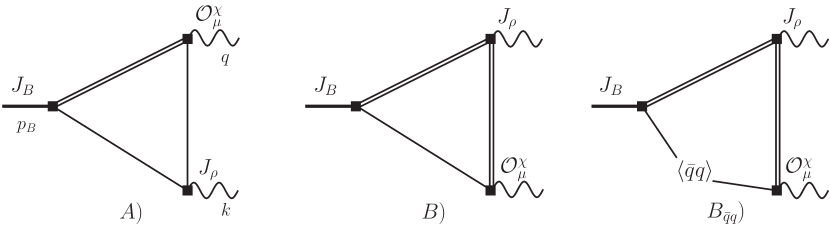
Figure 1: Perturbative diagrams of the A- and B-type as well as the B-type quark condensate diagram. The absence of the A-type quark condensate diagram, due its singular $1/k^{2}$-behaviour, is commented on in the main text. Throughout, single and double line denote light $q=u,d,s$- and a heavy $b$-quark respectively.

4.1.2 Next-to-leading Order

The most labour-intensive task of this work is the computation of the radiative corrections to the perturbative part. This computation is performed off-shell, $k^{2}\neq 0$, as it provides a regularisation to IR-divergences and we can make use of the NLO basis of master integrals DiVita:2017xlr . With three external momenta and one internal mass, intended for $X^{0}\rightarrow W^{+}W^{-}$ with $X^{0}=\{H,Z,\gamma^{*}\}$, they are state-of-the-art if the method of differential equations in massive 2-loop integrals.

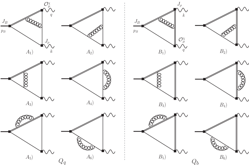
Figure 2: Radiative corrections to the perturbative contribution to the form factors. Diagrams $A_{1-6})$ and $B_{1-6})$ are proportional to the charges $Q_{q}$ and $Q_{b}$ respectively.

The diagrams are depicted in Fig. 2 with the additional derivative diagrams in Fig. 3. After evaluating the traces in FeynCalc FeynCalc1 ; FeynCalc2 scalar products of momenta are efficiently replaced with propagator denominators via the LiteRed litered:2013 package, and then reduced to master integrals by Kira kira:2017 . The master integrals (MIs) are expressed in terms of multiple-polylogarithms (MPLs), cf. App. F. The $k^{2}\to 0$ limit is taken and thereafter the discontinuities for the dispersion representation (17) are found using the PolyLogTools polylogtools package. We extended the basis of MIs in DiVita:2017xlr to include those that are given by the swapping of external legs. Whereas technically this leads to an over-complete basis, this was necessary in order to perform both the renormalisation and the $k^{2}\to 0$ limit efficiently where cancellation of the IR-divergent $\ln k^{2}$-terms takes place. We have included these MIs as an ancillary file to the arXiv version. All integrals, including the new MIs, have been numerically verified against pySecDec pySecDec1 ; pySecDec2 and PolyLogTools polylogtools .

Following this executive summary we give some more detail below. With the help of LiteRed, scalar products of loop and external momenta appearing in the numerators of the integrals depicted in the diagrams of Fig. 2 are written in terms of propagator denominators such that all integrals are reduced to the following form

$$\text{MI}[T,\{n_{1},n_{2},n_{3},n_{4},n_{5},n_{6},n_{7}\}]=\int d^{d}\ell_{1}\int d^{d}\ell_{2}\frac{1}{D_{T1}^{n_{1}}\,D_{T2}^{n_{2}}\,D_{T3}^{n_{3}}\,D_{T4}^{n_{4}}\,D_{T5}^{n_{5}}\,D_{T6}^{n_{6}}\,D_{T7}^{n_{7}}}\;,$$ (34)

with $n_{i}\in\mathbb{Z}$ and $T\in\{A,B\}$. For the A-type basis, corresponding to diagrams proportional to the light-quark charge $Q_{q}$, the propagator denominators are

$$D_{A1} =\ell_{1}^{2}, D_{A2} =\ell_{2}^{2}, D_{A3} =(\ell_{1}+p_{B})^{2}-m_{b}^{2},\qquad D_{A4}=(\ell_{2}+p_{B})^{2}-m_{b}^{2},$$

$$D_{A5} =(\ell_{1}+k)^{2}, D_{A6} =(\ell_{2}+k)^{2}, D_{A7} =(\ell_{1}-\ell_{2})^{2},$$ (35)

and for the B-type basis, corresponding to diagrams proportional to the heavy-quark charge $Q_{b}$, we have,

$$D_{B1} =\ell_{1}^{2}-m_{b}^{2}\;, D_{B2} =\ell_{2}^{2}-m_{b}^{2}\;, D_{B3} =(\ell_{1}-p_{B}+k)^{2}\;,$$

$$D_{B4} =(\ell_{2}-p_{B}+k)^{2}\;, D_{B5} =(\ell_{1}+k)^{2}-m_{b}^{2}\;, D_{B6} =(\ell_{2}+k)^{2}-m_{b}^{2}\;,$$

$$D_{B7} =(\ell_{1}-\ell_{2})^{2}\;,$$ (36)

with the usual $i0$-prescription implied. We note that the A-type and B-type diagrams correspond to the $(a)$-$(b)$ and $(c)$-$(d)$ topologies in DiVita:2017xlr . The corresponding MPLs are of weight $1$ to $4$ as is appropriate for a 2-loop computation. The additional MIs that we compute are:

$$\text{MI}[B,\{0,2,1,0,1,1,1\}]\;,\qquad\text{MI}[B,\{0,1,2,0,1,1,1\}]\;,\qquad\text{MI}[B,\{0,1,1,0,1,1,1\}]\;,$$

$$\text{MI}[B,\{0,2,2,0,1,1,1\}]\;,\qquad\text{MI}[B,\{1,0,1,1,2,2,0\}]\;,\qquad\text{MI}[B,\{0,0,1,1,2,2,0\}]\;.$$ (37)

The bare $\Pi^{\parallel,\perp}$ are subject to renormalisation. Besides the standard renormalisation of the $b$-quark mass in connection with the self-energy graphs, one need to renormalise the operators of the correlation function. The electromagnetic current does not renormalise, $Z_{J_{b}}=Z_{m_{b}}$ and the renormalisation of the weak operators (4) is discussed in App. C.2. In particular the renormalisation of $O^{D}_{\mu}$ provides a rather non-trivial test of the computation. After this we perform the $k^{2}\to 0$ limit and take the discontinuities aided by PolyLogTools. In order to do this efficiently we use shuffle algebra relations, such as

$$G(a,b,z)\,G(c,z)=G(a,b,c,z)+G(a,c,b,z)+G(c,a,b,z),$$ (38)

to reorganise the result into a linear sum of MPLs. The task of computing the discontinuity of the correlation function then becomes one of computing the discontinuity of each individual MPL with details given in App. F. It should be emphasised that the $Q_{b}$-type MIs are much more involved than the $Q_{q}$-ones, which is also mirrored in their alphabet length of $18$ and $10$ respectively DiVita:2017xlr .

The final step in the computation of the perturbative densities is to translate the MPLs into the more familiar classical polylogs. In doing so we move from complicated functions with relatively simple branch cut structures, to simple functions with complicated branch cut structures. Consequently, the representation of a given MPL in terms of polylogs depends on the regions in which its arguments lie, meaning that a single expression may not be sufficient to span all possible values of the arguments. An explicit example of this can be seen in Eq.$(4.2)$ of Frellesvig:2016ske . We have numerically verified that the perturbative densities written in terms of classical polylogs are equivalent to those given in terms of MPLs in the region of interest, $q^{2}<m_{b}^{2}<p_{B}^{2}$.

Figure 3: Additional diagrams required when computing the correlation function $\Pi_{\mu}^{\mathcal{D}}$.

4.2 The light-cone OPE diagrams of Twist-$2$,$3$ and $4$

In phenomenology the light-cone OPE has its roots in deep inelastic scattering, which is an inclusive measurement where the operators on the light-cone are the parton distribution functions $\langle P(p)|\bar{q}(z)\Gamma q(0)|P(p)\rangle$. The Fourier transform of the light-cone direction $p^{-}z^{+}$ describes the probability of finding a constituent parton of a certain momentum fraction. The application of the light-cone OPE to hard exclusive processes CZ1984 is a different matter, as the light-cone operators correspond to DAs, e.g. $\langle 0|\bar{d}(z)\Gamma u(0)|\pi^{+}(p)\rangle$ and the Fourier transform in the light-cone direction, denoted by the variable $u$ in this work, describes the amplitude for each parton having momentum fraction $u$. We refer the reader to the technical review Braun:2003rp where the connection to conformal symmetry is presented in depth and detail.

In a concrete setting an OPE is associated with factorisation. The light-cone OPE corresponds to collinear factorisation and is often schematically presented (in momentum space) as

$$\Pi(q^{2},m_{b})=\sum_{i}T^{(i)}_{H}(q^{2},m_{b},\mu_{F})\otimes\phi_{i}(\mu_{F})\;,$$ (39)

where $\Pi$ is the correlation function, $T^{(i)}_{H}$ a perturbatively calculable hard scattering kernel, $\phi_{i}$ a DA, $\otimes$ denotes the integration over the collinear momentum fractions (suppressed in the formula), $\mu_{F}$ is the factorisation scale and the sum runs over DAs of increasing twist. A necessary condition for factorisation to hold is that the $\mu_{F}$-dependence cancels to the given order in a computation. This corresponds to the absorption of collinear IR-divergences of the hard kernel into the DAs. We will discuss this explicitly in Sec. 4.2.3.

4.2.1 Quark Mass Correction to the Photon Distribution Amplitude

This section serves to illustrate the leading twist-$2$ photon DA and we present a method to incorporate quark mass corrections, which are sizeable in the case of the strange quark. The leading twist-2 photon DA is given by (D.4)

$$\langle\gamma(k,\epsilon)|\bar{q}(0)\sigma_{\alpha\beta}q(z)|0\rangle\;=\;is_{e}eQ_{q}\langle\bar{q}q\rangle\chi\epsilon^{*}_{[\alpha}k_{\beta]}\int_{0}^{1}due^{i\bar{u}kz}\phi_{\gamma}(u,\mu)+\textrm{higher twist}\;,$$ (40)

where the Wilson line is omitted for brevity and $\chi$ is known as the magnetic vacuum susceptibility, which serves as a normalisation of the photon DA in the sense that $f^{\perp}_{\gamma}=\langle\bar{q}q\rangle\chi$ is the analogue of the transverse decay constant $f_{\rho}^{T}$ for a $\rho$-meson. Its value without the inclusion of quark mass effects (and thus no quark subscript) is $\chi\approx 3\,\mbox{GeV}$, at the scale $\mu=1\,\mbox{GeV}$, known from QCD sum rules Ioffe:1983ju ; Ball:2002ps and lattice computations Bali:2012jv ; Bali:2020bcn .

For finite quark mass $m_{q}$ the local matrix element is UV-divergent. More precisely, it mixes with the identity (additive renormalisation) which is symptomatic of any OPE. Thus including finite quark mass corrections requires a specific prescription which we propose. Our starting point is the non-local matrix element for an off-shell photon $\gamma^{*}(k^{2}\neq 0)$

$$\langle\gamma^{*}(k,\epsilon)|\bar{q}(0)\sigma_{\alpha\beta}q(x)|0\rangle \;=\; -ie\epsilon_{\mu}^{*}\int e^{iky}\langle 0|Tj^{\mu}(y)\bar{q}(0)\sigma_{\alpha\beta}q(x)|0\rangle=$$ (41)

$$\;=\; is_{e}eQ_{q}\epsilon^{*}_{[\alpha}k_{\beta]}\int_{0}^{1}due^{i\bar{u}kx}\Phi_{\gamma^{*}}(u,k^{2},x^{2})\;,$$

where we parameterise ($\mu$-dependence suppressed)

$$\Phi_{\gamma^{*}}(u,k^{2},x^{2})=\langle\bar{q}q\rangle\chi\phi_{\gamma}(u,k^{2})+\frac{N_{c}m_{q}}{4\pi^{2}}\phi^{(m_{q})}_{\gamma^{*}}(k^{2},x^{2})\;,$$

and remind the reader that, by definition, $\chi$ does not include quark mass corrections. The LO contribution is straightforward to compute

$$\phi^{(m_{q})}_{\gamma^{*}}(k^{2},x^{2}) \;=\; -2K_{0}\left(\sqrt{(m_{q}^{2}-u\bar{u}k^{2})(-x^{2}+i0)}\,\right)+{\cal O}(\alpha_{s})$$ (42)

$$\;=\; \ln\left(\frac{m_{q}^{2}-\bar{u}uk^{2}}{4\mu^{2}}\right)+\ln(-x^{2}+i0)\mu^{2}+2\gamma_{E}+{\cal O}(\alpha_{s},x^{2})\;,$$

where $K_{0}$ is the modified Bessel function of the second kind. The $\ln(-x^{2}+i0)$-term signals the UV-divergence which is regulated by $x^{2}\neq 0$. Upon taking the local limit from the start and using DR $d=4-2\epsilon$, we identity at LO $1/\epsilon_{\textrm{UV}}+\ln 4\pi-\gamma_{E}\leftrightarrow-\ln\frac{(-x^{2}+i0)\mu^{2}}{4}-2\gamma_{E}$.

Before discussing the LO-prescription to remove the UV-divergence, let us digress on the sign of the $\ln(-x^{2}+i0)$-term. Some time ago Ioffe and Smilga Ioffe:1983ju analysed the local matrix element using a UV cut-off $\Lambda$ and a constituent quark mass. Taking into consideration their sign convention of $\chi<0$, we expect an increase of $\Lambda^{2}\leftrightarrow 1/x^{2}$ to effectively enhance $\chi$ (recall $\langle\bar{q}q\rangle<0$ for $m_{q}>0$). The same remark applies to the evaluation of this quantity in the background of a constant magnetic field via its Dirac eigenvalues cf. App. B in Bali:2012jv . Hence our sign is in accordance with these treatments.

We would like to motivative the LO-prescription. The Fourier transform of $\ln(-x^{2})$

$$\mu^{d-4}\int d^{d}xe^{ipx}\ln(-x^{2}\mu^{2})=i(4\pi)^{2}\frac{1}{p^{4}}+{\cal O}(\epsilon)$$ (43)

corresponds to a zero momentum insertion approximation. We have checked by explicit computation that this leads to the same result when one uses a mass-insertion approximation in perturbation theory. Hence at LO in $\alpha_{s}$ dropping the $\ln(-x^{2}\mu^{2})$-term is the correct prescription in order to avoid double counting. Whether dropping solely the $\ln(-x^{2}\mu^{2})$-term is the correct prescription for higher order or not is an open question and deserves further exploration.

Now that the UV-divergent part is separated it remains to be seen what we can do with the DA piece

$$\phi^{(m_{q})}_{\gamma^{*}}(k^{2})=\phi^{(m_{q})}_{\gamma^{*}}(k^{2},x^{2})|_{\textrm{twist--2}}=\ln(-\bar{u}uk^{2}/(4\mu^{2}))+2\gamma_{E}\;.$$ (44)

If one could trust the $k^{2}\to 0$ limit then one could simply add it to the twist-$2$ DA $\Phi^{(\phi_{\gamma})}_{\gamma}$ with $\phi^{(m_{q})}_{\gamma^{*}}(0)$ in place. Clearly this is not the case since perturbation theory is not applicable for $k^{2}\to 0$ as illustrated by the singularity. A well-known solution to this problem is to invoke a dispersion relation Ball:2002ps . We can build on their work for determining $\chi$ in the massless quark limit and add our contribution. The only relevant conceptual difference is that we have to use a once-subtracted dispersion relation because of the logarithmic divergence.

It was found in Ball:2002ps that the sum rules for higher moments are unstable and we thus focus on the zeroth moment $\chi_{q}$ (recall $f^{\perp}_{\gamma q}=\langle\bar{q}q\rangle\chi_{q}$). The once subtracted dispersion representation reads

$$f^{\perp}_{\gamma^{*}q}(k^{2})=\int_{0}^{1}du\Phi^{(m_{q})}_{\gamma^{*}}(u,k^{2})=f^{\perp}_{\gamma^{*}q}(k_{0}^{2})+\int_{\textrm{cut}}^{\infty}\frac{dr\,\rho^{f^{\perp}_{\gamma^{*}q}}(r)}{r-k^{2}-i0}R(r)\;,$$ (45)

with $R(r)=\frac{k^{2}-k_{0}^{2}}{r-k_{0}^{2}}$ and $\pi\rho^{f^{\perp}_{\gamma^{*}s}}=\textrm{Im}f^{\perp}_{\gamma^{*}s}$.

Assuming the quark content ($|\rho_{0}[\omega]\rangle\simeq(|\bar{u}u\rangle\mp|\bar{d}d\rangle)/\sqrt{2}$ and $|\phi\rangle\simeq|\bar{s}s\rangle$) and adopting the zero width approximation we may rewrite the dispersion relation as follows

$$f^{\perp}_{\gamma^{*}s}(k^{2}) \;=\; f^{\perp}_{\gamma^{*}s}(k_{0}^{2})+\frac{m_{\phi}f_{\phi}f_{\phi}^{T}}{m_{\phi}^{2}-k^{2}-i0}R(m_{\phi}^{2})+\int_{r^{(\phi)}_{0}}^{\infty}\frac{dr\,\rho^{f^{\perp}_{\gamma^{*}s}}(r)}{r-k^{2}-i0}R(r)\;,$$

$$f^{\perp}_{\gamma^{*}q}(k^{2}) \;=\; f^{\perp}_{\gamma^{*}q}(k_{0}^{2})+\frac{m_{\rho}f_{\rho}f_{\rho}^{T}}{m_{\rho}^{2}-k^{2}-i0}R(m_{\rho}^{2})+\int_{r^{(\rho)}_{0}}^{\infty}\frac{dr\,\rho^{f^{\perp}_{\gamma^{*}q}}(r)}{r-k^{2}-i0}R(r)\;,$$ (46)

where $r_{0}$ is the hadronic threshold due to higher states and we have adopted the isospin limit $f^{\perp}_{\gamma^{*}q}\equiv f^{\perp}_{\gamma^{*}u}\approx f^{\perp}_{\gamma^{*}d}$. Now, in order to evaluate the RHS, besides the decay constants $(f_{\rho},f_{\rho}^{T})=(0.220(5),0.160(7))\,\mbox{GeV}$, $(f_{\phi},f_{\phi}^{T})=(0.233(4),0.191(4))\,\mbox{GeV}$ BSZ15 and continuum thresholds $(r_{0}^{(\rho)},r_{0}^{(\phi)})=(1.5(1),2.0(1))\,\mbox{GeV}^{2}$ Ball:2002ps , one needs the subtraction constant and the spectral density $\rho(r)$. Both of these can be obtained from the local OPE $f^{\perp}_{\gamma^{*}s}(k^{2})$. Using the results in App. B in Ball:2002ps and adding our $m_{q}$-correction we find

$$f^{\perp}_{\gamma^{*}q}(k^{2})=\frac{2\langle\bar{q}q\rangle}{k^{2}}\left(-1+C_{F}\frac{\alpha_{s}}{\pi}(1-\ln\frac{-k^{2}}{\mu^{2}})-\frac{1}{3}\frac{m_{0}^{2}}{k^{2}}\right)+\frac{N_{c}m_{q}}{4\pi^{2}}\left(2(\gamma_{E}-1)-\ln 4+\ln\frac{-k^{2}}{\mu^{2}}\right)\;,$$ (47)

where $\langle\bar{q}\sigma\!\cdot\!Gq\rangle=m_{0}^{2}\langle qq\rangle$ with $m_{0}^{2}=0.8(2)\,\mbox{GeV}^{2}$. The spectral function

$$\rho^{f^{\perp}_{\gamma^{*}s}}(s)=\frac{2C_{F}\alpha_{s}}{\pi}\frac{\langle\bar{q}q\rangle}{s}-\frac{N_{c}m_{q}}{4\pi^{2}}\;,$$ (48)

is obtained from (47). Using $\chi_{q}=f^{\perp}_{\gamma q}/\langle\bar{q}q\rangle$ and adopting the notation $f^{\perp}_{\gamma q}=f^{\perp}_{\gamma^{*}q}(0)$ with reference to (4.2.1) we find (with $\mu=1\,\mbox{GeV}$)

$$f_{\gamma q}^{\perp} \;=\; -48(3)\,\mbox{MeV}\quad \Leftrightarrow \quad\chi_{q} \;=\; 3.21(15)\,\mbox{GeV}^{-2}\;,\quad$$

$$f_{\gamma s}^{\perp} \;=\; -61(3)\,\mbox{MeV}\;,\quad \Leftrightarrow \quad\chi_{s} \;=\; 3.79(17)\,\mbox{GeV}^{-2}\;,$$ (49)

where we have kept $-k_{0}^{2}>3\,\mbox{GeV}^{2}$ in the deep Euclidean region as appropriate for a short distance expansion. In addition we quote an $SU(3)$-ratio

$$r_{SU(3)}=\frac{f_{\gamma s}^{\perp}}{f_{\gamma q}^{\perp}}=1.28(4)\;.$$ (50)

All results are highly stable with respect to the subtraction point $k_{0}^{2}$ which is a sign of consistency in both the formula and its input, as the individual parts show sizeable variation (for $k_{0}^{2}\in[2,10]\,\mbox{GeV}^{2}$ the results vary less than a percent). The value of (50) corresponds to a typical $SU(3)$-ratio in the non-perturbative realm. The $m_{s}$-contribution in perturbation theory can be estimated to be of the order of $m_{s}/m_{b}\approx 0.02$ and can therefore be dropped.

We wish to emphasise that whereas $\chi_{q}(f_{\gamma q})$ merely reproduces the result in Ball:2002ps (within minor variation of the input), $\chi_{s}(f_{\gamma s})$ is the first determination of this quantity. The quantity $\chi_{s}$ in Bali:2012jv ; Bali:2020bcn should not be compared to the $\chi_{s}$ above as it differs in the renormalisation prescription. We re-emphasise that our prescription emerges naturally from the twist expansion. The fact that a correction to a non-perturbative matrix element can be computed with perturbative methods is somewhat exceptional and so let us comment. A key difference to QCD condensates or matrix elements is that $f^{\perp}_{\gamma q}$ is of mass dimension one which is taken by the quark mass. In QCD this would involve ${\cal O}(\Lambda_{\textrm{QCD}}^{n})$-terms. The remaining logarithmic divergence $\ln\Lambda_{\textrm{QCD}}$ can be absorbed into the perturbative part (twist-$1$).

4.2.2 Leading Order

The LO graphs, corresponding to the light-cone DA contributions to the FFs are depicted in Fig. 4. The expansion is performed up to twist-$4$, including $3$-particle DAs, with the definition of the DAs given in App. D. As mentioned above the $Q_{q}\langle\bar{q}q\rangle$-term is part of this expansion cf. Eq. (D.1) to see this explicitly.

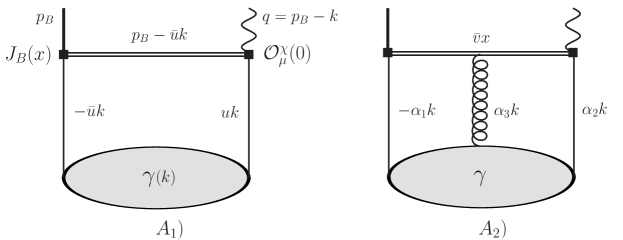
Figure 4: LO contributions in the DAs. $A_{1})$ $2$-particle DA $A_{2})$ $3$-particle DA. The variable $u\in[0,1]$ and $\bar{u}=1-u$ are the momentum fractions carried by quarks. The point $vx$, $v\in[0,1]$, corresponds to the gluon in the background field gauge propagator (D.3). The $\alpha_{i}$ denote the momentum fractions of the quarks and gluon with $\alpha_{1}\!+\!\alpha_{2}\!+\!\alpha_{3}\!=\!1$.

4.2.3 Next-to-leading Order

Further to the LO graphs we have also computed the twist-$2$ ${\cal O}(\alpha_{s})$ corrections in the photon DA $\phi_{\gamma}(u)$. The relevant diagrams are depicted in Fig. 5, with additional diagrams for $\Pi^{D}_{\mu\rho}$ shown in Fig. 6, and the total results given in App. E.3 in terms of Passarino-Veltman (PV) functions. A noticeable feature is that in the Feynman gauge the box diagram $A_{3})$ vanishes.

Figure 5: $\mathrm{O}(\alpha_{s})$ corrections to twist-$2$ DA contribution. $A_{1}$) vertex-correction $A_{2}$) $J_{B}$-correction $A_{3}$) box-diagram $A_{4-6}$) $b$- and $q$-quark self energy corrections.

For the radiative corrections there are issues with regard to IR- and UV-divergences to be discussed. A particularly clear discussion of these matters can be found in B83 . First, the necessary conditions for collinear factorisation to hold are (i) that there are no divergences on integration over the collinear momentum fraction $u$ and (ii) that the collinear IR-divergences can be absorbed into the bare DA, $\phi^{\textrm{bare}}_{\gamma}$, which is not observable. We find that our integrals converge when integrated over $u$ therefore satisfying the first condition. The collinear IR-divergences are absorbed into the LO DA. For this to be possible the divergences have to assume the following form $T_{H,1}^{\textrm{div}}=c\,T_{H,0}\otimes V_{0}$. In this equation $T_{H,0(1)}$ are the LO and NLO hard scattering amplitudes, $V_{0}$ is the LO Efremov-Radyushkin-Brodsky-Lepage evolution kernel Efremov:1978rn ; Efremov:1979qk ; Lepage:1980fj and $c$ is a constant or simply the counterterm B83 . One may use the property that the eigenfunctions and eigenvalues of $V_{0}^{\perp}$ are known Shifman:1980dk

$$V^{\perp}_{0}\otimes\varphi_{n}=\int_{0}^{1}V^{\perp}_{0}(u,v)\varphi_{n}(v)=-\gamma_{n}^{(0)\perp}\varphi_{n}(u)\;,$$ (51)

with

$$\varphi_{n}(u)=6u\bar{u}\,C^{(3/2)}_{n}(2u-1)\;,\quad\gamma_{n}^{(0)\perp}=2C_{F}\left(1+4\sum_{j=2}^{n+1}\frac{1}{j}\right)\;,$$ (52)

where $C_{F}=(N_{c}^{2}-1)/(2N_{c})$ and $C^{(3/2)}_{n}(x)$ is the $n^{\textrm{th}}$ Gegenbauer polynomials of degree $3/2$. The divergencies can then be absorbed into

$$\phi_{\gamma}^{\textrm{bare}}=6u\bar{u}\sum_{n\geq 1}(a_{n}^{\perp})^{\textrm{bare}}C^{(3/2)}_{n}(2u-1)\;,\quad$$ (53)

where

$$(a_{n}^{\perp})^{\textrm{bare}}=(\mu/\mu_{0})^{2\epsilon}a_{n}^{\perp}(\mu)\left(1+c\frac{g^{2}}{(4\pi)^{2}}\gamma_{n}^{(0)\perp}\frac{1}{\epsilon}\right)\;.$$ (54)

Requiring

$$0=\frac{d}{d\ln\mu}(a_{n}^{\perp})^{\textrm{bare}}=a_{s}\gamma_{n}^{(0)\perp}(-1+2c)\;,\quad a_{s}=g^{2}/(4\pi)^{2}\;,$$ (55)

determines $c=\frac{1}{2}$. This is indeed the constant that we find in our explicit computation and thus shows $\mu_{F}$-independence and cancellation of the collinear IR-divergences. This is not a new result as the computation is equivalent to the $\phi^{\perp}$-amplitude in $\bar{B}\to V$ FFs where it was verified at the twist-$2$ level in BB98b ; BZ04b and for the $V^{\bar{B}_{u}\to\gamma}$ in Ball:2003fq .

Figure 6: Additional diagrams originating from the emission of the photon from the $\mathcal{O}_{\mu}^{D}$-operator. In principle there are two additional graphs, one for perturbation theory and for $\overline{Q}\langle\bar{q}q\rangle$, where the photon is emitted from the covariant derivative of the $O^{D}_{\mu}$-vertex. However, these graphs turn out to be proportional to $\epsilon^{*}_{\mu}$ and are orthogonal to our projection prescription (28), and we therefore do not include them. Further not that if they were truly missing the EOM would not close.

Obtaining the dispersion representation (17) of the twist-$2$ NLO contribution is not straightforward from the representation given in (E.10), which we write schematically

$$\Pi_{\perp}(p_{B}^{2})=\int_{0}^{1}du\pi_{\perp}(u,p_{B}^{2})\;,$$ (56)

with $\pi_{\perp}(u,p_{B}^{2})=T_{\perp}(u,p_{B}^{2})\phi_{\gamma}(u)$. Whereas the function $\Pi_{\perp}(p_{B}^{2})$ has a cut starting at $m_{b}^{2}$, $\pi_{\perp}(u,p_{B}^{2})$ has additional cuts in the $(u,p_{B}^{2})$-variables. Two natural choices present themselves. Firstly, one commits to a certain form of the twist-$2$ photon DA and integrates over $du$ in (56) such that the (poly)logs are functions of the external kinematic variables only and one can then obtain the discontinuity in the standard way. The other possibility is that one uses the fact that a FF’s discontinuity is equivalent to its imaginary part. One may write, working with a single subtraction term at $p_{B}^{2}=\bar{s}$ in order to regulate the logarithmic UV-divergence,

$$\Pi^{V}_{\perp}(p_{B}^{2})-\Pi^{V}_{\perp}(\bar{s}) \;=\; \frac{(p_{B}^{2}-\bar{s})}{\pi}\int_{m_{b}^{2}}^{\infty}\frac{ds}{s-\bar{s}}\frac{\textrm{Im}[\int_{0}^{1}du\pi^{V}_{\perp}(u,s)]}{s-p_{B}^{2}-i0}$$ (57)

$$\;\stackrel{{\scriptstyle p_{B}^{2}<m_{b}^{2}}}{{=}}\; \textrm{Im}\left[\frac{(p_{B}^{2}-\bar{s})}{\pi}\int_{\Gamma_{1}}\frac{ds}{s-\bar{s}}\frac{\int_{\Gamma_{2}}du\pi_{\perp}^{V}(u,s)}{s-p_{B}^{2}}\right]\;,$$

where $\Gamma_{1,2}$ are paths distorted into the upper complex planes $\mathbb{C}_{s,u}$ to avoid singularities. We have validated this procedure numerically.

In the final dispersion integral, after Borel transformation, the recipe reads

$$V_{\perp}(q^{2})=\frac{1}{f_{B}m_{B}^{2}}\textrm{Im}\left[\frac{1}{\pi}\int_{\Gamma_{m_{b}^{2},s_{0}}}dse^{(m_{B}^{2}-s)/M^{2}}\int_{\Gamma_{2}}du\pi_{\perp}^{V}(u,s,q^{2})\right]\;,$$ (58)

where the integration endpoint of $\Gamma_{1}$, which is $\infty$, is moved to the continuum threshold $s_{0}$. This integral is numerically very stable.

4.3 Comparison of Form Factor computation with the Literature

The twist-$1$ and $2$ LO results agree with Khodjamirian:1995uc ; Ali:1995uy . At twist-$3$ and $4$ we can compare with Ball:2003fq and find that the $\langle\bar{q}q\rangle$, ${\cal U}$, $\mathbb{A}$, $S_{\gamma}$ & $T_{4\gamma}$ contributions are missing and our result in $\tilde{S}$ is larger by a factor of six. At NLO solely the twist-$2$ result has been reported in Ball:2003fq ; Wang:2018wfj . In the first reference it is presented only in numeric form and the agreement is reasonable taking into account the slightly different numerical input. In Wang:2018wfj analytic results are given but there is a sign difference between the twist-$1$ and the twist-$2$ term (cf. their figure 5) in contrast to our result. To continue the discussion at this point it is useful to already take into account some of our numerical results of the proceeding section. Correcting for the mentioned sign, and taking into account the global sign difference (7), focusing on twist-$1$ and $2$ one gets $V^{\bar{B}_{u}\to\gamma}_{\perp}|_{\mbox{\cite[cite]{\@@bibref{Authors Phrase1YearPhrase2}{Wang:2018wfj}{\@@citephrase{(}}{\@@citephrase{)}}}}}\approx-(0.28_{t=1}+0.08_{t=2})=-0.36$ whereas we find $V^{\bar{B}_{u}\to\gamma}_{\perp}\approx-(0.124_{t=1}+0.082_{t=2})=-0.206$ (cf. Tab. 6). The discrepancy is too large in view of our ${\cal O}(10\%)$-uncertainty. In addition the value $V_{\perp}=-0.36$ is too large in view of the Belle exclusion limit (cf. Sec. 5.3). The breakdown suggests that the culprit is the twist-$1$ contribution for which two sources can be identified. First, the twist-$1$ result in Wang:2018wfj is only to leading power in $1/m_{b}$ and this suggests that the non-leading part is sizeable. Second, the not too well-known $B$-meson DA parameters and the assumption of a specific model for the DA itself (cf. the discussion in Sec. 5.4). To conclude, our analysis suggests that a posteriori the hybrid approach in Wang:2018wfj is numerically not sound because it does not include the full next-leading power corrections in the $1/m_{b}$-expansion.

4.4 Equations of Motion as a Test of the Computation

Generally EOM give rise to relations between correlation functions, cf. App. C which often involve CTs. For simple local FFs these CTs are absent and imply, in the case at hand, the following relations

$$T_{\perp}(q^{2})+{\cal D}_{\perp}(q^{2}) \;=\; \frac{(m_{b}+m_{q})}{m_{B}}V_{\perp}(q^{2})\;,$$

$$T_{\parallel}(q^{2})+{\cal D}_{\parallel}(q^{2}) \;=\; \frac{(m_{b}-m_{q})}{m_{B}}V_{\parallel}(q^{2})\;.$$ (59)

We wish to stress that these relations are completely general and thus have to be obeyed by any approach. We further note that the point-like part $f^{(pt)}_{B_{q}}$ (2.1) cancels between the LHS and RHS in the $\parallel$-equation.

Reassuringly, we find that (4.4) holds in all parameters for which we have complete results: perturbation theory (twist-$1$), $\{\chi\langle\bar{q}q\rangle,a_{2}(\gamma),a_{4}(\gamma)\}$ (twist-$2$), $f_{3\gamma}$ at LO in $1/m_{b}$ (twist-$3$) and $Q_{b}\langle\bar{q}q\rangle$ (twist-$4$ local OPE). For twist-$1$ and $2$ this includes the NLO correction in $\alpha_{s}$. There are some comments to be made on the other cases. The parameter $f_{3\gamma}$ is defined from a $3$-particle matrix element of twist-$3$ but could mix into a $4$-particle matrix element. This effect is $1/m_{b}$-suppressed, which we have checked analytically, and fortunately numerically negligible. The only true twist-$4$ term that we include is $Q_{b}\langle\bar{q}q\rangle$ and now turn to the reason why, which has to our knowledge not been thoroughly discussed in the literature.

It concerns the consistent inclusion of twist-$4$ $3$-particle DA parameters. Our finding is that this demands $4$-particle DAs and is based on the following two observations. Firstly, $4$-particle DAs of the form $\bar{q}(x)G_{\alpha\beta}(vx)G_{\gamma\delta}(ux)\sigma_{\rho\sigma}q(0)$, which do appear in the light-cone expansion of the propagator cf. eq. A.16 in Balitsky:1987bk , allow for twist-$4$ contributions. Secondly, these terms would mix via the EOM, generalisations of Eq. 4.40 Ball:2002ps , into the $3$-particle DAs of twist-$4$. The point is that the EOM at the FF-level need to close in each hadronic parameter separately, to be used in the numerics. In fact we find that of the $3$-particle twist-$4$ parameters only $\zeta_{2}^{+}$ closes and $\{\kappa,\kappa_{+},\zeta_{1},\zeta_{1}^{+},\zeta_{2}\}$ including the $\langle\bar{q}Fq\rangle$-type contributions (D.25) do not. As there is no argument as to whether any of the FF-combination are to be preferred over others we are led to conclude that one needs to drop those parameters altogether. Fortunately quite a few of them are zero (Tab. 1) and the numerical impact of the others is well below $10\%$ (Tab. 6). Whereas the numbers in the table seem higher for the charged $\bar{B}_{u}$, footnote 13 is relevant in that it probably means that the numbers are overestimated. Note that for the photon DA the omission of twist-$4$ parameters for the $3$-particle case then implies that the $2$-particle twist-$4$ DAs are effectively zero as their only contribution comes from the EOM with the $3$-particle DA of twist-$4$. This is different to the vector mesons where the $m_{V}^{2}$-contributions appear as $2$-particle ones of twist-$4$ and are sizeable for the $\phi$-meson for example BSZ15 .

5 Numerics

In this section we turn to the numerics for which we first discuss the input, the sum rule parameters, correlations of parameters due to the EOM and the fit-ansatz in Sec. 5.1. In Sec. 5.2 FF-plots, fit parameters and values for $q^{2}=0$ and are given in Fig. 7, Tab. 5 Tab. 4 respectively The correlation matrix can be found in an ancillary file to the arXiv version. The prediction of the $\bar{B}_{u}\to\gamma\ell^{-}\bar{\nu}$ rate with bins and correlation matrix is given in Sec. 5.3 In Sec. 5.4 we present the extraction of the $B$-meson DA parameter $\lambda_{B}$ by comparing to a set of three SCET-computations.

5.1 Input Parameters, Sum Rule Parameters and Fits

The input parameters, including the values for the photon DAs, are collected in Tab. 1. An important aspect is the choice of the mass scheme. The $\overline{\text{MS}}$- and the pole-scheme give rise to large effects in either higher twist or radiative corrections which suggests that neither is optimal (cf. Fig. 13 and Tab. 10). The kinetic scheme, originally developed for the OPE in inclusive decays Bigi:1994em , can be regraded as a compromise of these two schemes and we have found that it does indeed give rise to stable results. From Fig. 12 it is seen that this leads to stability in $\mu_{\textrm{kin}}$ with uncertainties in the $1$-$2\%$ range. To our knowledge this is the first time this scheme is used in the context of LCSR and we also adapt it in the closely related work on the $g_{BB^{*}\gamma}$-type on-shell couplings Pullin:2021ebn . The value of the kinetic mass, shown in Tab. 1, has been obtained using the two-loop relation between the $\overline{\text{MS}}$ and kinetic mass given in Gambino:2017vkx . The uncertainty on the kinetic mass has been estimated by adding the error on the $\overline{\text{MS}}$ mass and the one from the conversion formula (variation of scale $\mu_{m}\in[m_{b}/2,2m_{b}]$) in quadrature. In line with other applications we set the scale of the kinetic scheme to $\mu_{\textrm{kin}}\!=(\!1\pm 0.4)\,\mbox{GeV}$.

Running coupling parameters
$\alpha_{s}(m_{Z})\mbox{~{}\cite[cite]{\@@bibref{Authors Phrase1YearPhrase2}{PDG}{\@@citephrase{(}}{\@@citephrase{)}}}}$	$m_{Z}\mbox{~{}\cite[cite]{\@@bibref{Authors Phrase1YearPhrase2}{PDG}{\@@citephrase{(}}{\@@citephrase{)}}}}$
$0.1176(20)$	$91.19\,{\textrm{GeV}}$
Scales
$\mu_{F}^{B_{d,u}}=\mu_{\text{cond}}^{B_{d,u}}=\mu_{\alpha_{s}}^{B_{d,u}}$		$\mu_{F}^{B_{s}}=\mu_{\text{cond}}^{B_{s}}=\mu_{\alpha_{s}}^{B_{s}}$		$\mu_{\text{UV}}$	$\mu_{\textrm{kin}}$
$2.24(1.00)\,{\textrm{GeV}}$		$2.44(1.00)\,{\textrm{GeV}}$		$4.78(1.00)\,{\textrm{GeV}}$	$1.00(40)\,{\textrm{GeV}}$
$J^{P}=0^{-}\mbox{ Meson masses~{}\cite[cite]{\@@bibref{Authors Phrase1YearPhrase2}{PDG}{\@@citephrase{(}}{\@@citephrase{)}}}}$
$m_{B_{d}}$	$m_{B_{u}}$	$m_{B_{s}}$
$5.280\,{\textrm{GeV}}$	$5.280\,{\textrm{GeV}}$	$5.367\,{\textrm{GeV}}$
$J^{P}=1^{\pm}\mbox{ Meson masses~{}\cite[cite]{\@@bibref{Authors Phrase1YearPhrase2}{PDG}{\@@citephrase{(}}{\@@citephrase{)}}}}$
$m_{B^{*}_{d}}$	$m_{B^{*}_{u}}$	$m_{B^{*}_{s}}$	$m_{B_{1d}}$	$m_{B_{1u}}$	$m_{B_{1s}}$
$5.325\,{\textrm{GeV}}$	$5.325\,{\textrm{GeV}}$	$5.415\,{\textrm{GeV}}$	$5.726\,{\textrm{GeV}}$	$5.726\,{\textrm{GeV}}$	$5.829\,{\textrm{GeV}}$
Quark masses PDG
$m_{s{|2\!\,{\textrm{GeV}}}}$	$m_{b}(m_{b})$	$m_{b}^{\textrm{pole}}$	$m_{b}^{kin}(1\,{\textrm{GeV}})^{\dagger}$
$92.9(7)\,{\textrm{MeV}}$	$4.18(4)\,{\textrm{GeV}}$	$4.78(6)\,{\textrm{GeV}}$	$4.53(6)\,{\textrm{GeV}}$
Condensates
$\langle\bar{q}q\rangle_{|2\!\,{\textrm{GeV}}}\mbox{~{}\cite[cite]{\@@bibref{Authors Phrase1YearPhrase2}{Bali:2012jv}{\@@citephrase{(}}{\@@citephrase{)}}}}$	$\langle\bar{s}s\rangle\mbox{~{}\cite[cite]{\@@bibref{Authors Phrase1YearPhrase2}{McNeile:2012xh}{\@@citephrase{(}}{\@@citephrase{)}}}}$	$\langle G^{2}\rangle\mbox{~{}\cite[cite]{\@@bibref{Authors Phrase1YearPhrase2}{SVZ79I,SVZ79II}{\@@citephrase{(}}{\@@citephrase{)}}}}$	$m_{0}^{2}\mbox{~{}\cite[cite]{\@@bibref{Authors Phrase1YearPhrase2}{Ioffe:2002ee}{\@@citephrase{(}}{\@@citephrase{)}}}}$
$-(269(2)\,{\textrm{MeV}})^{3}$	$1.08(16)\langle\bar{q}q\rangle$	$0.012(4)\,{\textrm{GeV}}^{4}$	$0.8(2)\,{\textrm{GeV}}^{2}$
Photon distribution amplitude parameters
$f_{\gamma q{|1\!\,{\textrm{GeV}}}}^{\perp}\mbox{~{}\eqref{eq:fga}}$	$f_{\gamma s{|1\!\,{\textrm{GeV}}}}^{\perp}\mbox{~{}\eqref{eq:fga}}$	$f_{3\gamma{|1\!\,{\textrm{GeV}}}}\mbox{~{}\cite[cite]{\@@bibref{Authors Phrase1YearPhrase2}{Ball:2002ps}{\@@citephrase{(}}{\@@citephrase{)}}}}$	$\omega_{\gamma{|1\!\,{\textrm{GeV}}}}^{A}\mbox{~{}\cite[cite]{\@@bibref{Authors Phrase1YearPhrase2}{Ball:2002ps}{\@@citephrase{(}}{\@@citephrase{)}}}}$	$\omega_{\gamma{|1\!\,{\textrm{GeV}}}}^{V}\mbox{~{}\cite[cite]{\@@bibref{Authors Phrase1YearPhrase2}{Ball:2002ps}{\@@citephrase{(}}{\@@citephrase{)}}}}$
$-48(3)\,{\textrm{MeV}}$	$-61(3)\,{\textrm{MeV}}$	$-0.004(2)^{*}\,{\textrm{GeV}}^{2}$	$3.8(1.8)^{*}$	$-2.1(1.0)^{*}$
$\kappa_{|1\!\,{\textrm{GeV}}}\mbox{~{}\cite[cite]{\@@bibref{Authors Phrase1YearPhrase2}{Ball:2002ps}{\@@citephrase{(}}{\@@citephrase{)}}}}$	$\kappa^{+}_{|1\!\,{\textrm{GeV}}}\mbox{~{}\cite[cite]{\@@bibref{Authors Phrase1YearPhrase2}{Ball:2002ps}{\@@citephrase{(}}{\@@citephrase{)}}}}$	$\zeta_{1{|1\!\,{\textrm{GeV}}}}\mbox{~{}\cite[cite]{\@@bibref{Authors Phrase1YearPhrase2}{Ball:2002ps}{\@@citephrase{(}}{\@@citephrase{)}}}}$	$\zeta_{1{|1\!\,{\textrm{GeV}}}}^{+}\mbox{~{}\cite[cite]{\@@bibref{Authors Phrase1YearPhrase2}{Ball:2002ps}{\@@citephrase{(}}{\@@citephrase{)}}}}$	$\zeta_{2{|1\!\,{\textrm{GeV}}}}\mbox{~{}\cite[cite]{\@@bibref{Authors Phrase1YearPhrase2}{Ball:2002ps}{\@@citephrase{(}}{\@@citephrase{)}}}}$	$\zeta_{2{|1\!\,{\textrm{GeV}}}}^{+}\mbox{~{}\cite[cite]{\@@bibref{Authors Phrase1YearPhrase2}{Ball:2002ps}{\@@citephrase{(}}{\@@citephrase{)}}}}$
$0.2(2)$	$0(0)$	$0.4(4)$	$0(0)$	$0.3(3)$	$0(0)$

Table 1: Summary of input parameters. An asterisk, *, indicates that the quantity has been evaluated in the vector meson dominance approximation. Recall that $f_{\gamma q}=\chi_{q}{\left\langle\bar{q}q\right\rangle}$ where $\chi_{q}$ is the magnetic vacuum susceptibility of the quark condensate. The Gegenbauer moments of the photon DA, absent in this table, are discussed after (D.20) and set to $a_{2}(\gamma)=0(0.1)$ and $a_{4}(\gamma)=0(0)$. For the meson masses we have not indicated an error as they are negligible for this work. Although we do not use the twist-$4$ in the numerics, for reasons discussed in Sec. 4.4 we include their values in the table for completeness. The values of the $\kappa$ and $\zeta$-parameters are taken from the paper where the photon DA was first introduced Balitsky:1997wi , and estimated those matrix elements to be correct within a factor of two and note that the ones set to zero are systematically smaller. We have $\mu_{\alpha_{s}}^{2}=\mu_{F}^{2}\!=\!m_{B}^{2}\!-\!(m_{b}^{pole})^{2}$ and the renormalisation scale of the tensor current is set to $\mu_{\text{UV}}=m_{b}^{pole}$.

The sum rule specific parameters, given in Tab. 2, are determined by imposing a series of consistency conditions. Whilst we refrain from assigning a $q^{2}$ dependence to the SR parameters we consider the constraints set out below to apply for $q^{2}\in[0,7]\,\mbox{GeV}^{2}$. For the effective threshold $s_{0}$ it is required that the daughter SR, which is formally exact,

$$m_{B}^{2}=M^{4}\frac{d}{dM^{2}}\ln\int_{m_{b}^{2}}^{s_{0}}ds\;e^{-s/M^{2}}\rho(s,q^{2})\;,$$ (60)

reproduces the known $B$-meson mass to within $1$-$2\%$. The $SU(3)$ ratio of effective thresholds should approximately reproduce that of the meson masses $s_{0}^{B_{s}}/s_{0}^{B_{d,u}}\approx m_{B_{s}}^{2}/m_{B_{d,u}}^{2}$, which we use as an additional loose constraint. The Borel mass is obtained by considering two competing factors. A large Borel mass leads to faster convergence of the LC-OPE at the cost of greater contamination from the continuum states, whereas a small value of the Borel mass achieves exactly the opposite. We balance these two factors by requiring both that the continuum contributes no more than $30\%$ and that the highest twist contribution remains below $10\%$ of the result. Varying the Borel mass to $\pm 2\,\mbox{GeV}$ results in $1$-$2\%$ changes in the FF-value which is rather satisfactory. Next, we turn to correlations imposed by the EOM.

	$\bar{B}_{d}$	$\bar{B}_{u}$	$\bar{B}_{s}$
$\!\!\{s_{0},M^{2}\}^{V_{\perp},T_{\perp},T_{\parallel}}$	35.2(2.0), 8.0(2.0)	35.2(2.0), 8.0(2.0)	36.2(2.0), 8.0(2.0)
$\{s_{0},M^{2}\}^{V_{\parallel}}$	35.8(2.0), 8.5(2.0)	35.8(2.0), 8.5(2.0)	36.8(2.0), 9.5(2.0)
$\!\!\{s_{0},M^{2}\}^{f_{B}}$	34.3(2.0), 5.6(2.0)	34.3(2.0), 5.6(2.0)	35.5(2.0), 6.4(2.0)

Table 2: Summary of the sum rule parameters. The reason for not correlating the continuum thresholds for $T_{\parallel}$ and $V_{\parallel}$ is given in Sec. 5.1.1.

5.1.1 Equations of Motion as Constraints on Sum Rule Parameters

Besides providing a non-trivial check of both the computation and the formalism of the OPE and DAs itself cf. Sec. 4.4, the EOM serve an additional purpose in that they correlate the vector and tensor FF as the derivative FF turns out to be small. This observation was first made for the $B\to V$-FFs, with $V=\rho,\phi,...$ a light meson, in Hambrock:2013zya and more systematically exploited in BSZ15 . Numerically, the derivative FFs in (4.4) are suppressed by an order of magnitude as compared to the vector and tensor ones. This means that the sum rule specific parameters, of Borel mass and continuum threshold, ought to be approximately equal $s_{0}^{V}\simeq s_{0}^{T}$ and $M_{V}\simeq M_{T}$; otherwise this would imply an unprecedented violation of quark-hadron duality for the derivative FF.

Does this still hold for the $B\to\gamma$ FFs? Inspecting Tab. 5 we note that this pattern persists for the $\perp$-direction but not for the $\parallel$-direction. As the computation is a 1-to-1 formal map with the $B\to V$ FFs for higher twist-$2$ and above (cf. Tab. 11) this suggests that there is something special going on in the perturbative diagrams (twist-$1$ and $Q_{b}\langle qq\rangle$).

FF	$Q_{q}$ PT${}^{\text{ LO [NLO]}}$	$Q_{b}$ PT${}^{\text{ LO [NLO]}}$	$\chi\langle\bar{q}q\rangle^{\text{ LO [NLO]}}$	$f_{3\gamma}$	$Q_{b}\langle\bar{q}q\rangle$	$Q_{q}\langle\bar{q}q\rangle$
$V_{\perp}$	$m_{b}^{-1/2[-1/2]}$	$m_{b}^{-3/2[-3/2]}$	$m_{b}^{-3/2[-1/2]}$	$m_{b}^{-3/2}$	$m_{b}^{-3/2}$	$m_{b}^{-5/2}$
$V_{\parallel}$	$m_{b}^{-1/2[-1/2]}$	$m_{b}^{-3/2[-3/2]}$	$m_{b}^{-3/2[-1/2]}$	$m_{b}^{-3/2}$	$m_{b}^{-3/2}$	$m_{b}^{-5/2}$
$T_{\perp}$	$m_{b}^{-1/2[-1/2]}$	$m_{b}^{-3/2[-3/2]}$	$m_{b}^{-3/2[-1/2]}$	$m_{b}^{-5/2}$	$m_{b}^{-3/2}$	$m_{b}^{-5/2}$
$T_{\parallel}$	$m_{b}^{-1/2[-1/2]}$	$m_{b}^{-3/2[-3/2]}$	$m_{b}^{-3/2[-1/2]}$	$m_{b}^{-5/2}$	$m_{b}^{-3/2}$	$m_{b}^{-5/2}$
$D_{\perp}$	$m_{b}^{-3/2[-1/2]}$	$m_{b}^{-5/2[-3/2]}$	0 [$m_{b}^{-3/2}$]	$m_{b}^{-5/2}$	0	0
$D_{\parallel}$	$m_{b}^{-3/2[-1/2]}$	$m_{b}^{-3/2[-3/2]}$	0 [$m_{b}^{-3/2}$]	$m_{b}^{-5/2}$	$m_{b}^{-3/2}$	$m_{b}^{-3/2}$

Table 3: Heavy quark scaling of the form factors according to the rules in (61). The breaking of the hierarchy $V,T\gg{\cal D}$ at NLO is compatible with the findings in Beneke:2000wa . The $T,V_{\perp,\parallel}\propto Q_{q}m_{b}^{-1/2}$ and $T,V_{\perp,\parallel}\propto Q_{b}m_{b}^{-3/2}$ are discussed from a dispersion relation approach in Secs. 2.3 (Eq. (14)) and 5.1.1 respectively.

In order to understand the origin let us briefly recall how the FF-hierarchy can be understood in $B\to V$. We proceed by investigating the heavy quark limit of the FF. Whereas sum rules do not lend themselves to a heavy quark expansion, since some $m_{b}$ dependence is hidden in hadronic parameters, it is nevertheless possible to extract the leading $1/m_{b}$-behaviour by making the following well-known substitutions

$$m_{B}\to m_{b}+\bar{\Lambda}\;,\quad s_{0}\to(m_{b}+\omega_{0})^{2}\;,\quad M^{2}\to 2m_{b}\tau\;,$$ (61)

where $\bar{\Lambda},\omega_{0}$ and $\tau$ are all parameters of ${\cal O}(\Lambda_{\textrm{QCD}})$. For $B\to V$ it was observed that the derivative FFs are $1/m_{b}$-suppressed at ${\cal O}(\alpha_{s}^{0})$ Hambrock:2013zya ; BSZ15 . This pattern is broken at NLO where they show the same scaling. The $B\to\gamma$ scaling are collected in Tab. 3. The twist-$2$ parameter $\chi\langle\bar{q}q\rangle$, of course, confirms the earlier findings, whereas for twist-$1$ it is found that the hierarchy is obeyed in $Q_{q}$ but not $Q_{b}$. The former is in complete accord with the heavy quark scaling argument, presented in Sec. 2.3 where the $Q_{q}$-part is inferred as a sum of $B\to V_{n}$ FFs. As for the latter we can offer a similar argumentation as in Secs. 2.3, Eq. (14), by using the dispersion representation in the limit of large colours

$$T^{\bar{B}_{s}\to\gamma}_{\perp}(q^{2})|_{Q_{b}}=\sum_{V_{n}=\Upsilon,\Upsilon^{\prime},\dots}\frac{f^{\textrm{e}m}_{V_{n}}}{m_{V_{n}}}\,T_{1}^{\bar{B}_{s}\to V_{n}}(q^{2})+\textrm{s.t.}\;,$$ (62)

where we focus on the resonances for simplicity. The heavy quark scaling

$$(m_{V_{n}},f^{\textrm{e}m}_{V_{n}},T_{1}^{V_{n}\to\bar{B}_{s}}(0))\propto(m_{b},m_{b}^{-1/2},m_{b}^{0})\;,$$ (63)

of the hadronic parameters are all trivial. In fact each generic term in (62) scales like $m_{b}^{-3/2}$. Contrary to the case for the $Q_{q}$-charge, there is no obvious significant alteration for the sum when scaling in $m_{b}$ and we conclude $T^{\bar{B}_{s}\to\gamma}_{\perp}(q^{2})|_{Q_{b}}\propto m_{b}^{-3/2}$, which is indeed consistent with our findings cf. Tab. 3. This explains the scaling but also makes it clear that the $Q_{b}$-part has nothing to do with light vector mesons and the ideas behind the large energy limit are thus not applicable. Hence there is no reason to believe that such a hierarchy is in place and the pattern in Tab. 5 is now qualitatively understood. We consider it instructive to give a numeric breakdown for the LO contributions up to twist-$2$

$$V^{\bar{B}_{q}\to\gamma}_{\parallel}(0) \;\simeq\; (-0.01\,Q_{b} \;-\; 0.09\,Q_{q})|_{\text{PT}} \;-\; 0.11\,Q_{q}|_{\text{twist-2}} \;+\; \textrm{higher twist}\;,$$

$$T^{\bar{B}_{q}\to\gamma}_{\parallel}(0) \;\simeq\; (-0.03\,Q_{b} \;-\; 0.17\,Q_{q})|_{\text{PT}} \;-\; 0.09\,Q_{q}|_{\text{twist-2}} \;+\; \textrm{higher twist}\;,$$

$${\cal D}^{\bar{B}_{q}\to\gamma}_{\parallel}(0) \;\simeq\; (\phantom{-}0.02\,Q_{b} \;+\; 0.10\,Q_{q})|_{\text{PT}} \;+\; \phantom{0.0}0\,Q_{q}|_{\text{twist-2}} \;+\; \textrm{higher twist}\;,$$

$$V^{\bar{B}_{q}\to\gamma}_{\perp}(0) \;\simeq\; (-0.03\,Q_{b} \;-\; 0.17\,Q_{q})|_{\text{PT}} \;-\; 0.11\,Q_{q}|_{\text{twist-2}} \;+\; \textrm{higher twist}\;,$$

$$T^{\bar{B}_{q}\to\gamma}_{\perp}(0) \;\simeq\; (-0.03\,Q_{b} \;-\; 0.17\,Q_{q})|_{\text{PT}} \;-\; 0.09\,Q_{q}|_{\text{twist-2}} \;+\; \textrm{higher twist}\;,$$

$${\cal D}^{\bar{B}_{q}\to\gamma}_{\perp}(0) \;\simeq\; (\phantom{-}0.00\,Q_{b} \;+\; 0.03\,Q_{q})|_{\text{PT}} \;+\; \phantom{0.0}0\,Q_{q}|_{\text{twist-2}} \;+\; \textrm{higher twist}\;,$$ (64)

where $q=u,d$. Above we see that whilst the derivative FF is small in the $\perp$-direction it provides a considerable contribution in the $\|$-direction, and is the reason we allow the central values of the continuum thresholds of $V_{\parallel}^{\bar{B}\to\gamma}$ and $T_{\parallel}^{\bar{B}\to\gamma}$ to differ, in contrast to the other FFs. Moreover the numerical suppression of ${\cal D}^{\perp}$ in perturbation theory might or might not be accidental. In view of these findings we apply a moderate (smaller than in $B\to V$ BSZ15 ) correlation of the tensor versus vector thresholds. Further to the correlations induced by the EOM, the effective thresholds of the FFs and the decay constant are correlated, which is warranted as both thresholds are associated with the $B$-meson state

$$\text{corr}(s_{0}^{V^{q}_{\|[\perp]}},s_{0}^{T^{q}_{\|[\perp]}})=0.5\;,\quad\text{corr}(s_{0}^{\Gamma^{q}_{\|[\perp]}},s_{0}^{f_{B}})=0.5\;,$$ (65)

where $q=u,d,s$ and $\Gamma=V,T$.

5.1.2 Fit-ansatz

A generic FF, say $F_{n}$, is fitted to a $z$-expansion ansatz, following the same setup as in previous work BSZ15 ; Albrecht:2019zul , where the leading pole is factored out

$$F_{n}^{\bar{B}\to\gamma}(q^{2})=\frac{1}{1-q^{2}/m_{R}^{2}}\left(\alpha_{n0}+\sum_{k=1}^{N}\alpha_{nk}(z(q^{2})-z(0))^{k}\right)\;.$$ (66)

The variable $z$ describes the following map into the complex plane: $z(t)=\frac{\sqrt{t_{+}-t}-\sqrt{t_{+}-t_{0}}}{\sqrt{t_{+}-t}+\sqrt{t_{+}-t_{0}}}$ ($t_{0}\equiv t_{+}(1-\sqrt{1-t_{-}/t_{+}})$, $t_{\pm}\equiv(m_{B_{q}}\pm m_{\rho})^{2}$ and $m_{\rho}=770\,\mbox{MeV}$). It is noted that $t_{\pm}\to m_{B_{q}}\pm 2m_{\pi},m_{B_{s}}\pm 2m_{K}$ is formally correct but we use $t_{\pm}$ as above with no impact on our results in the physical region. We note that whilst $t_{+}$ corresponds to the multiparticle production threshold, the choice of $t_{0}$ (and therefore $t_{-}$) is arbitrary and does not impact our results. The masses of the lowest lying $J^{P}=1^{-(+)}$ states, relevant to the $\perp(\parallel)$-projection, are $m_{R}=m_{B^{*}_{q}(B_{1q})}$.

Relations between the FFs provide constraints on the fit parameters. For example (6) implies

$$T^{\bar{B}\to\gamma}_{\perp}(0)=T^{\bar{B}\to\gamma}_{\parallel}(0)\;\;\Leftrightarrow\;\;\alpha_{T_{\perp}0}=\alpha_{T_{\parallel}0}\;.$$ (67)

Further constraints arise from the dispersion representation. Considering the vector FF for concreteness,

$$V^{\bar{B}\to\gamma}_{\parallel[\perp]}(q^{2})=\frac{1}{\pi}\int^{\infty}_{\textrm{cut}}dt\frac{\textrm{Im}[V^{\bar{B}\to\gamma}_{\parallel[\perp]}(t)]}{t-q^{2}-i0}=\frac{r^{V}_{\parallel[\perp]}}{1-q^{2}/m_{B^{*}[B_{1}]}^{2}}+\dots\;,$$ (68)

one can infer the residue of the lowest-lying resonance

$$r^{(V,T)}_{\perp}\;=\;\left(\frac{m_{B}f_{B^{*}}}{m_{B^{*}}},f^{T}_{B^{*}}\right)g_{BB^{*}\gamma}\;,\quad r^{(V,T)}_{\parallel}\;=\;\left(\frac{m_{B}f_{B_{1}}}{m_{B_{1}}},f^{T}_{B_{1}}\right)g_{BB_{1}\gamma}\;,$$ (69)

with some more detail in Pullin:2021ebn along with the definition of the decay constants $f_{B^{*},B_{1}}^{(T)}$ and the on-shell matrix elements $g_{BB^{*}(B_{1})\gamma}$ describing the $B^{*}(B_{1})\to B\gamma$ transition. This relation enforces the constraint

$$r_{V_{\perp}}=\alpha_{V_{\perp}0}+\sum_{k=1}^{N}\alpha_{V_{\perp}k}(z(m_{B^{*}_{q}}^{2})-z(0))^{k}\;,$$ (70)

and similar constraints for other FFs. The main idea of the fit is that the four FFs with $15$ $q^{2}$-points (ranging from $[0,14]\,\mbox{GeV}^{2})$ and $N_{\text{samples}}=2500$ samples are subjected to a single fit providing correlations between the fit parameters of the FFs. This is the same Markov Chain Monte Carlo methodology as used in BSZ15 . Data points are generated from normal distributions correlated as in (65), with the exception of $\{\mu_{F},\mu_{\text{cond}},\mu_{\alpha_{s}},\mu_{\text{kin}},M^{2},M_{f_{B}}^{2}\}$ for which a skew normal distribution is applied. The latter is necessary since clearly not all parameters have a symmetric validity-range. The skew normal distribution is defined by three parameters, which we take to be the mean, the standard deviation and a shape parameter, $\alpha_{\text{shape}}$. The latter is chosen such that the probability of generating a sample below a certain cut-off is less than $10^{-4}$. For the scales we impose $\{\mu_{F},\mu_{\text{cond}},\mu_{\alpha_{s}}\}>0.8\,\mbox{GeV}$ and $\mu_{\text{kin}}>0.2\,\mbox{GeV}$ whilst for the Borel parameters we require $M^{2}>4\,\mbox{GeV}^{2}$ and $M^{2}_{f_{B}}>2\,\mbox{GeV}^{2}$, below which the twist expansion is non-convergent. The fitted FFs reproduce the mean values of generated FF data sets to within $\approx 0.5\%$ over the fitted region. The values of the fit parameters are given in Tab. 4, with some more description in the caption. Covariance and correlation matrices along with the central values of the fit-parameters are given as ancillary file appended to the arXiv version of this paper. The JSON formatted file is ordered according to charge, statistical quantity and FF(s) of interest and can be readily used in Mathematica. For example, after loading the data

	$V_{\perp}^{\bar{B}_{d}\to\gamma}$	$V_{\perp}^{\bar{B}_{s}\to\gamma}$	$V_{\perp}^{\bar{B}_{u}\to\gamma}$	$T_{\perp}^{\bar{B}_{d}\to\gamma}$	$T_{\perp}^{\bar{B}_{s}\to\gamma}$	$T_{\perp}^{\bar{B}_{u}\to\gamma}$
$\alpha_{0}$	$\phantom{\text{-}}0.133(17)$	$\phantom{\text{-}}0.158(18)$	$\text{-}0.213(26)$	$\phantom{\text{-}}0.133(13)$	$\phantom{\text{-}}0.151(13)$	$\text{-}0.213(19)$
$\alpha_{1}$	$\text{-}0.123(66)$	$\text{-}0.459(200)$	$\phantom{\text{-}}0.278(155)$	$\text{-}0.093(362)$	$\text{-}0.284(357)$	$\phantom{\text{-}}0.240(545)$
$\alpha_{2}$	$\phantom{\text{-}}1.280(913)$	$\phantom{\text{-}}1.798(1.303)$	$\text{-}1.760(1.486)$	$\phantom{\text{-}}1.075(3.277)$	$\phantom{\text{-}}2.489(3.356)$	$\text{-}1.346(4.707)$
$\alpha_{3}$	$\phantom{\text{-}}3.373(2.485)$	$\phantom{\text{-}}6.603(3.283)$	$\text{-}4.940(4.016)$	$\phantom{\text{-}}2.764(6.493)$	$\phantom{\text{-}}7.288(6.915)$	$\text{-}3.848(9.281)$
	$V_{\|}^{\bar{B}_{d}\to\gamma}$	$V_{\|}^{\bar{B}_{s}\to\gamma}$	$V_{\|}^{\bar{B}_{u}\to\gamma}$	$T_{\|}^{\bar{B}_{d}\to\gamma}$	$T_{\|}^{\bar{B}_{s}\to\gamma}$	$T_{\|}^{\bar{B}_{u}\to\gamma}$
$\alpha_{0}$	$\phantom{\text{-}}0.081(9)$	$\phantom{\text{-}}0.104(9)$	$\text{-}0.151(18)$	$\phantom{\text{-}}0.133(13)$	$\phantom{\text{-}}0.151(13)$	$\text{-}0.213(19)$
$\alpha_{1}$	$\text{-}0.138(53)$	$\text{-}0.177(63)$	$\phantom{\text{-}}0.312(129)$	$\text{-}0.071(377)$	$\text{-}0.237(359)$	$\phantom{\text{-}}0.230(535)$
$\alpha_{2}$	$\phantom{\text{-}}0.803(769)$	$\phantom{\text{-}}1.882(649)$	$\text{-}1.749(1.260)$	$\phantom{\text{-}}1.241(3.207)$	$\phantom{\text{-}}1.841(3.139)$	$\text{-}1.397(4.340)$
$\alpha_{3}$	$\phantom{\text{-}}1.986(1.408)$	$\phantom{\text{-}}3.951(1.220)$	$\text{-}4.263(2.314)$	$\phantom{\text{-}}2.746(4.768)$	$\phantom{\text{-}}4.180(4.684)$	$\text{-}3.472(6.397)$

Table 4: Fit parameters. To obtain the fits we generate $2500$ random samples of the input parameters, normally distributed such that for a given parameter the mean of the total sample set corresponds to the central value and the standard deviation to the uncertainty. The fit parameters $\alpha_{n}$ are then produced by fitting the data set generated by evaluating the form factors at integer values of $q^{2}\in[0,14]\,\mbox{GeV}^{2}$ for each sample to the ansatz (66) with $N=3$.

data$=$Import[…/BtoGam_FF.json]

all information can be accessed via the OptionValue command. For example, the central value of $\alpha_{T_{\perp}0}^{\bar{B}_{u}}$ is obtained with

OptionValue[data, "Bu"$\to$"central"$\to$"Tperp"$\to$"a0"] .

Similarly the correlation between $\alpha_{V_{\|}0}^{\bar{B}_{u}}$ and $\alpha_{T_{\|}2}^{\bar{B}_{u}}$ can be accessed via

OptionValue[data, "Bu"$\to$"correlation"$\to$"VparaTpara"$\to$"a0a2"] .

The uncertainty and covariance matrix are accessed in an analogous manner.

5.2 Results and Plots

The central values of the FFs (2.1) at $q^{2}=0$ and the residues (69) are given in Tab. 5. Plots of the neutral $\bar{B}_{d}$-, $\bar{B}_{s}$- and charged $\bar{B}_{u}$-modes are shown in Fig. 7. Together with the fit-values given in Tab. 4 of the previous section and the correlation matrix given in an ancillary file this constitutes the main practical results of our paper.

A breakdown of contributions, split according to twist and DAs, is given in Tab. 6. We remind the reader that all twist-$4$ contributions, other than the $Q_{b}{\left\langle\bar{q}q\right\rangle}$ condensates, are dropped as they require the inclusion of $4$-particle DAs cf. Sec. 4.4. This effect which is fortunately well below $10\%$ as can inferred from Tab. 5.

	$V_{\perp}(0)$	$V_{\|}(0)$	$T_{\perp,\|}(0)$
$\!\!\bar{B}_{d}$	$0.130(17)$	$0.079(9)\phantom{0}$	$0.129(17)$	$-$
$\bar{B}_{s}$	$0.160(18)$	$0.105(10)$	$0.153(16)$	$-$
$\bar{B}_{u}$	$-0.209(26)$	$-0.148(18)$	$-0.209(26)$	$-$
	$r_{\perp}^{V}$	$r_{\parallel}^{V}$	$r_{\perp}^{T}$	$r_{\parallel}^{T}$
$\!\!\bar{B}_{d}$	$\phantom{-}0.179(19)$	${0.076}(16)$	${0.171}(20)$	${0.104}(15)$
$\bar{B}_{s}$	$\phantom{-}0.235(25)$	${0.114}(18)$	${0.224}(24)$	${0.146}(17)$
$\bar{B}_{u}$	$-0.300(34)$	${-0.159}(31)$	${-0.284}(33)$	${-0.199}(28)$

Table 5: Values of the form factors (2.1) at $q^{2}=0$ along with the residues (69) evaluated in the kinetic scheme, cf. Pullin:2021ebn . Values for the threshold and Borel mass can be found in Tab. 2. All other input parameters are given in Tab. 1.

Whereas formally the fit-parameter $\alpha_{0}$ equals the FF-value at $q^{2}=0$, on comparison with Tab. 5 we see a deviation of ${\cal O}(2\%)$ between the two. This comes as the FFs are evaluated analytically whereas the fit-values follow from the Monte Carlo Markov-chain analysis ($N_{\text{samples}}=2500$ random samples) and the deviations are due to slightly asymmetric distribution of the uncertainty.

From the plots one infers the typical behaviour of a FF. Its value at $q^{2}=0$ is below the normalisation of a current, e.g. the electromagnetic pion FF $f_{+}^{\pi\to\pi}(0)=1$ and it raises as a result of hadronic poles (or multiquark thresholds in partonic QCD). One sees that the constraint from the first pole is well in line with the raise reproduced in our computation for $q^{2}\approx 14\,\mbox{GeV}^{2}$ and would become progressively worse. In the tensor case the $\perp$- and $\parallel$-directions only show significant deviations for large $q^{2}$, with the coincidence at $q^{2}=0$ enforced by (6). For the vector FFs this pattern would be reproduced if the derivative FFs were small. However, this is not the case in the $\|$-direction, as the vector form factor differ more notably (cf. (5.1.1) and the discussion of Sec. 5.1.1). Furthermore, we find that for both the twist-2 and leading $1/m_{b}$ twist-1 contribution (proportional to $Q_{q}$ only) the $\perp$- and $\parallel$-directions give identical results. Hence any degree of asymmetry between $\perp$ and $\parallel$ must arise from sub-leading perturbative and/or higher twist contributions. Our decision to drop hadronic parameters that do not close under the EOM from the analysis (cf. Sec. 4.4) therefore acts to increase the symmetry between the two directions.

twist	pa	DA	$V_{\perp}^{\bar{B}_{u}}(0)$	$V_{\perp}^{\bar{B}_{d}}(0)$	$V_{\|}^{\bar{B}_{u}}(0)$	$V_{\|}^{\bar{B}_{d}}(0)$	$T_{\perp,\|}^{\bar{B}_{u}}(0)$	$T_{\perp,\|}^{\bar{B}_{d}}(0)$	$T_{\perp,\|}^{\bar{B}_{s}}(0)$
1	-	$\textrm{PT}\,{\cal O}{(\alpha_{s}^{0})}$	$-0.104$	$0.065$	$-0.054$	$0.032$	$-0.105$	$0.065$	$0.086$
1	-	$\textrm{PT}\,{\cal O}{(\alpha_{s})}$	$-0.024$	$0.019$	$-0.010$	$0.006$	$-0.027$	$0.021$	$0.021$
2	2	$\phi_{\gamma}(u)\,{\cal O}{(\alpha_{s}^{0})}$	$-0.072$	$0.036$	$-0.073$	$0.037$	$-0.062$	$0.031$	$0.037$
2	2	$\phi_{\gamma}(u)\,{\cal O}{(\alpha_{s})}$	$-0.010$	$0.005$	$-0.011$	$0.006$	$-0.011$	$0.005$	$0.007$
3	2	$\Psi_{(a)}(u)$	$-0.002$	$0.001$	–	–	$-0.001$	$<\!10^{-3}$	$-0.003$
3	2	$\Psi_{(v)}^{(1)}(u)$	–	–	$-0.003$	$0.001$	$-0.002$	$0.001$	$-0.001$
3	3	$\mathcal{A}(\underline{\alpha})$	–	–	–	–	$-0.002$	$0.001$	$<\!10^{-3}$
3	3	$\mathcal{V}(\underline{\alpha})$	–	–	–	–	$-0.001$	$<\!10^{-3}$	$<\!10^{-3}$
4	2	$h_{\gamma}^{(2)}(u)$	–	–	$0.011$	$-0.005$	$0.004$	$-0.002$	$-0.002$
4	2	$\mathbb{A}(u)$	$0.015$	$-0.007$	$0.014$	$-0.007$	$0.011$	$-0.005$	$-0.005$
4	3	$S(\underline{\alpha})\!+\!\tilde{S}(\underline{\alpha})$	$<\!10^{-3}$	$<\!10^{-3}$	$<\!10^{-3}$	$<\!10^{-3}$	$-0.001$	$<\!10^{-3}$	$<\!10^{-3}$
4	3	$\sum\limits_{{i=1}}^{4}T_{i}^{(1)}(\underline{\alpha})$	$-0.002$	$0.001$	$-0.002$	$0.001$	$-0.004$	$0.002$	$0.002$
4	3	$S_{\gamma}$	$0.003$	$0.003$	$-0.002$	$-0.002$	$0.003$	$0.001$	$0.003$
4	3	$T_{4}^{\gamma}$	$<\!10^{-3}$	$<\!10^{-3}$	$<\!10^{-3}$	$<\!10^{-3}$	$<\!10^{-3}$	$<\!10^{-3}$	$<\!10^{-3}$
4	-	$Q_{q}\left\langle\bar{q}q\right\rangle$	–	–	$0.010$	$0.002$	–	–	–
4	-	$Q_{b}\left\langle\bar{q}q\right\rangle$	$0.004$	$0.004$	$0.003$	$-0.003$	$0.003$	$0.003$	$0.003$
		Total∗	$-0.194$	$0.127$	$-0.118$	$0.067$	$-0.197$	$0.127$	$0.151$

Table 6: A breakdown of contributions for a representative selection of form factors according to associated twist, “pa” = number of partons and DAs. The asterisk in total is a reminder that it includes twist-$4$ contributions that do not close under the EOM (cf. Sec. 4.4). The definitions of the DAs can be found in App. D. Results are given in the kinetic scheme with the kinetic scale $\mu_{\textrm{kin}}=1\,\mbox{GeV}$.

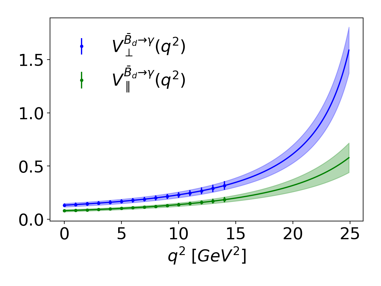
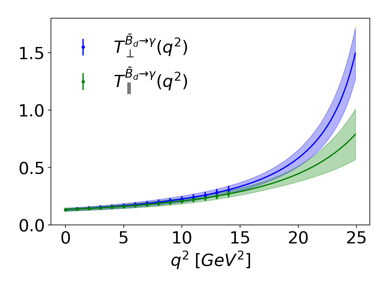
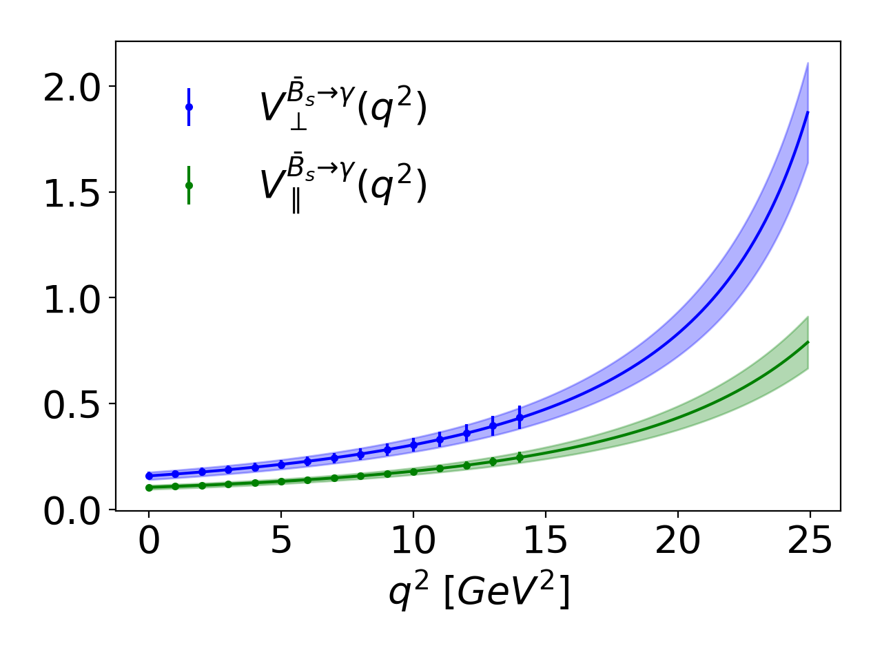
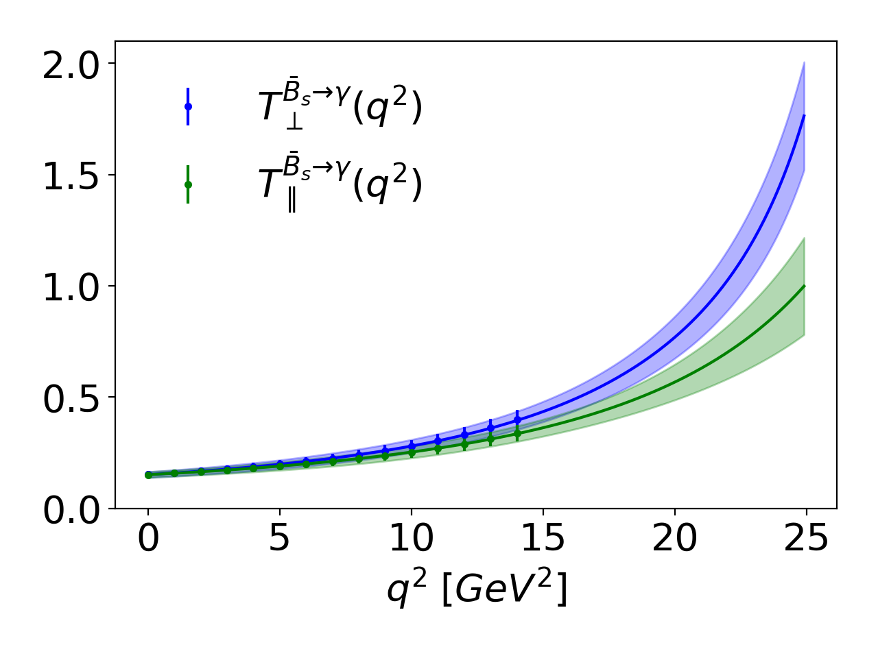
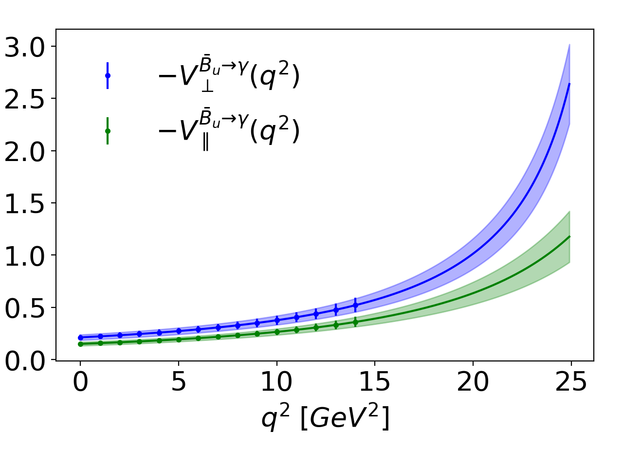
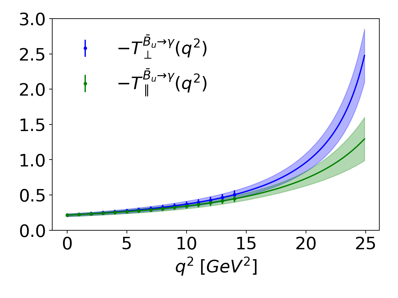
Figure 7: Form factors for the $\bar{B}_{d,s,u}\to\gamma$ transition where the data points (with solid bars as respective uncertainties) have been generated by a $N_{\text{samples}}=2500$ sample and fitted to the ansatz (66). The plots are reproduced from the fit-values in Tab. 4 and the uncertainty bands stem from the correlation matrix given as an ancillary file cf. Sec. 5.1 for further details. Whereas we consider the LCSR computation valid up to $q^{2}<14\,\mbox{GeV}^{2}$, the ansatz (66) with the pole residue from Pullin:2021ebn allows one to extend the form factor beyond this region. The sign of the charged form factors is reversed so that they are positive. We refer the reader to App. 2.1.1 for discussion of conventions.

5.2.1 Comparison with the Literature

In this section we compare our FFs to some of the results in the literature. Comparison with SCET computations of these FFs Beneke:2020fot is not straightforward as the $B$-meson DA parameters are not known with a lot of certainty. It is therefore advisable to turn the tables and use our predictions to set bounds as done in Sec. 5.4. Comments on comparison in terms of analytic computations can be found at the beginning of App. E. Lattice results are available for $D_{d,s}\to\gamma$ and $K,\pi\to\gamma$ modes in Desiderio:2020oej and in preparation by another group Kane:2019jtj . At low photon recoil such computations are of importance for QED-corrections. Whereas we have chosen not to present $D\to\gamma$ FFs, the pole residues of the vector FFs, $g_{DD^{*}\gamma}$, are computed in our other work Pullin:2021ebn and are consistent with experiment in the measured modes. A notable aspect is that the shape in Desiderio:2020oej does not seem to be compatible with the $D^{*}$-pole playing a significant role close to the kinematic endpoint of $D\to\gamma\ell\bar{\nu}$ ($q^{2}=m_{D}^{2}$).

We can, however, compare to the quark model computations MN04 ; Kozachuk:2017mdk (with $T^{\bar{B}_{d}\to\gamma}_{\perp,\parallel}=F^{\bar{B}_{d}\to\gamma}_{T_{V,A}}$ dictionary). Two representative plots of the neutral modes are given in Fig. 8. There is rather good agreement at low $q^{2}$ but we can clearly see that our FFs are larger for higher $q^{2}$ which ought have a significant impact on phenomenology.

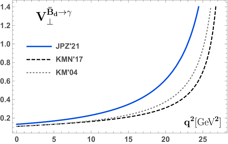
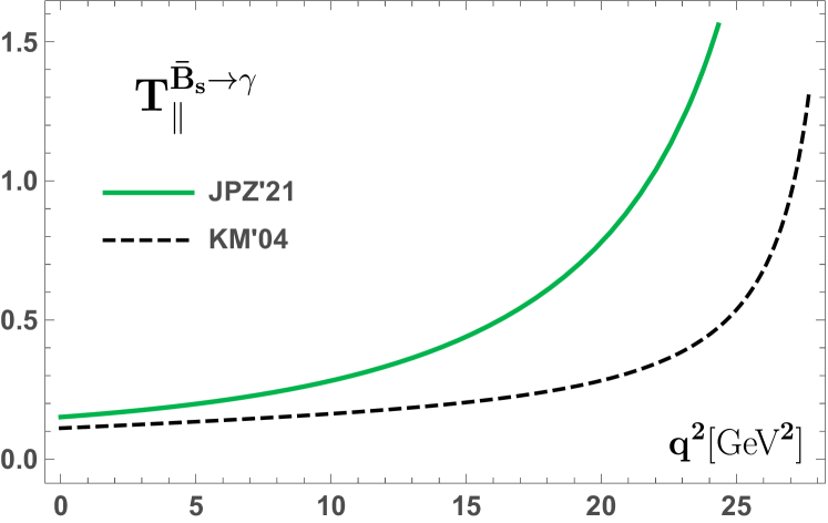
Figure 8: Representative comparison plots for neutral modes. Our plots (solid,blue/green) , denoted by JPZ, compared against the quark model computation MN04 (short-dashed,light grey) from 2004 and an improved version Kozachuk:2017mdk (dashed,black) with the modified pole version. Note that there are $\bar{B}_{s}\to\gamma$ results in the 2004 work. Our results are larger and, in particular, show an earlier rise. In view of this the numerical agreement of the central value at $V^{\bar{B}_{d}\to\gamma}_{\perp}(0)$ seems somewhat accidental.

For illustrative purposes we have added Fig. 9 comparing the form factor with and without the point-like contribution added.

Figure 9: Plot comparing the $V_{\parallel}^{\bar{B}_{u}\to\gamma}$ form factor, as defined in (2.1), with and without the inclusion of the point-like contribution $Q_{\bar{B}}f^{(pt)}_{\bar{B}_{u}}$. The value of the decay constant $f_{B}=190\,\mbox{MeV}$ is taken from Pullin:2021ebn (cf. references therein). The point-like term provides a significant contribution, most notably towards the $q^{2}=m_{B}^{2}$ pole.

5.3 Predictions for the $\bar{B}_{u}\to\gamma\ell^{-}\bar{\nu}$ Rate

The $\bar{B}_{u}\to\gamma\ell^{-}\bar{\nu}$ decay proceeds via a charged current and depends on the local FF only. Neglecting the lepton mass, anticipating a measurement in the electron mode, the differential rate after integrating over the lepton angle is given by

$$\frac{d\Gamma}{dE_{\gamma}}=\frac{G^{2}_{F}\alpha|V_{\textrm{ub}}|^{2}}{6\pi^{2}}m_{B}E_{\gamma}^{3}\left(1-\frac{2E_{\gamma}}{m_{B}}\right)\left(|V_{\perp}|^{2}+|V_{\parallel}|^{2}\right)\;,$$ (71)

where $E_{\gamma}=(m_{B}^{2}-q^{2})/(2m_{B})\in[0,\frac{m_{B}}{2}]$ is the photon energy in the $B$-meson restframe, such that $\frac{d\Gamma}{dq^{2}}=-\frac{1}{2m_{B}}\frac{d\Gamma}{dE_{\gamma}}$. We refer the reader to App. B.3 for an explanation of why the point-like part, proportional to $f_{B}$, disappears in the $m_{\ell}\to 0$ limit.

Plots of the branching fraction are shown, in both the $q^{2}$ and the $E_{\gamma}$ variables, in Fig. 10. The $q^{2}$ and $E_{\gamma}$ covariance matrices between the bins of Tab. 7 are respectively given by

$$\text{cov}_{\text{bin}}^{q^{2}}\!=\!\!\left(\!\begin{array}[]{cccc}0.0534&0.0502&0.0459&0.0393\\ 0.0502&0.0471&0.0431&0.0369\\ 0.0459&0.0431&0.0394&0.0337\\ 0.0393&0.0369&0.0337&0.0289\\ \end{array}\!\right),\quad\text{cov}_{\text{bin}}^{E_{\gamma}}\!=\!\left(\!\!\begin{array}[]{cccc}0.5537&0.4521&0.3188&0.1787\\ 0.4521&0.3736&0.2675&0.1523\\ 0.3188&0.2675&0.1954&0.1133\\ 0.1787&0.1523&0.1133&0.0669\\ \end{array}\!\right).$$ (72)

The $\bar{B}_{u}\to\gamma\ell^{-}\bar{\nu}$ rate will, finally, be measured at Belle II Kou:2018nap . A $90\%$ confidence level (CL), ${\cal B}(\bar{B}_{u}\to\gamma\ell^{-}\bar{\nu})_{E_{\gamma}>1\,\mbox{GeV}}<3.0\cdot 10^{-6}\;@90\%\textrm{ CL}$, with Belle data has been reported two years ago Gelb:2018end . This limit is about a factor of two above our predictions of $1.60(37)\cdot 10^{-6}$ given in Tab. 7.

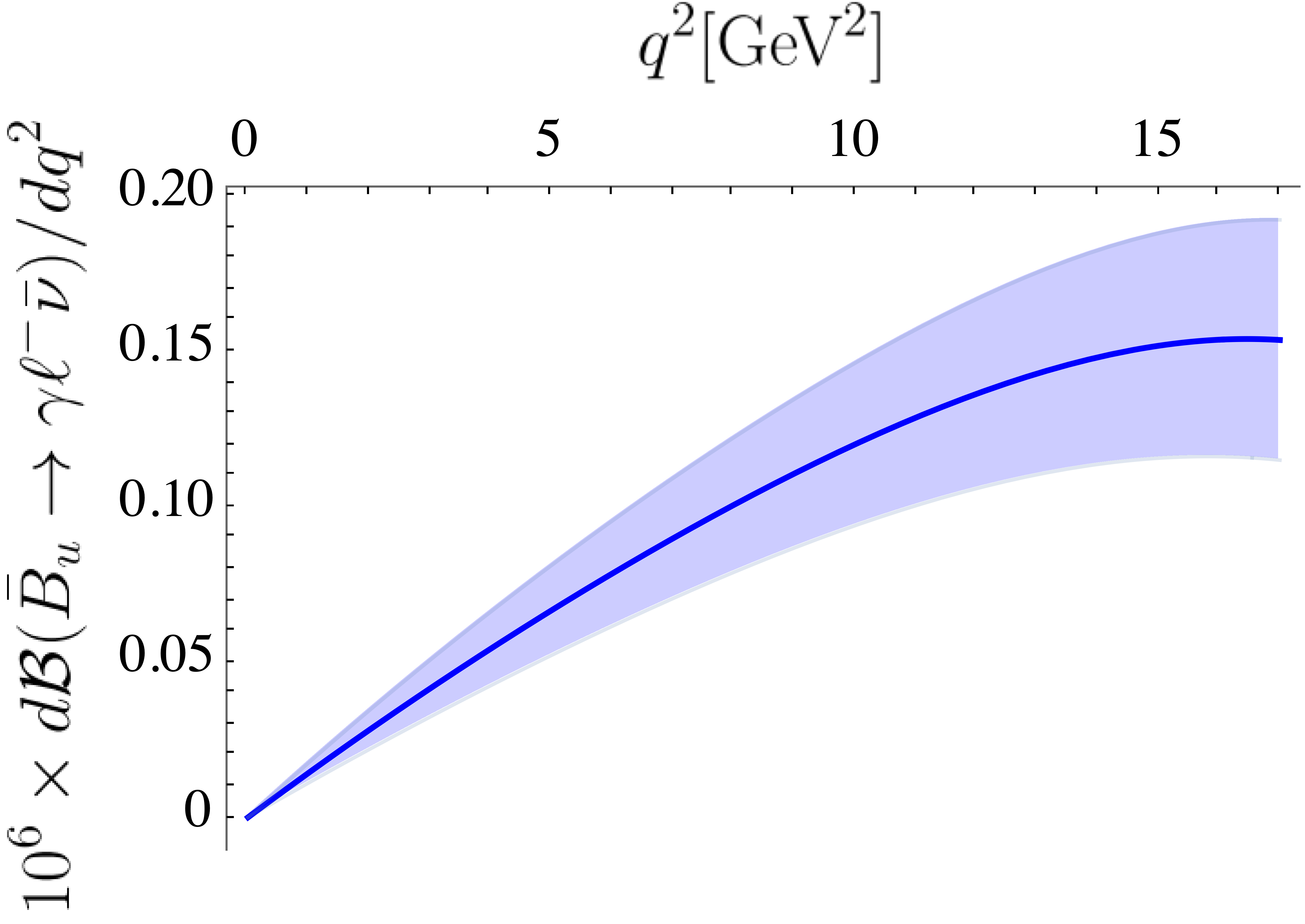
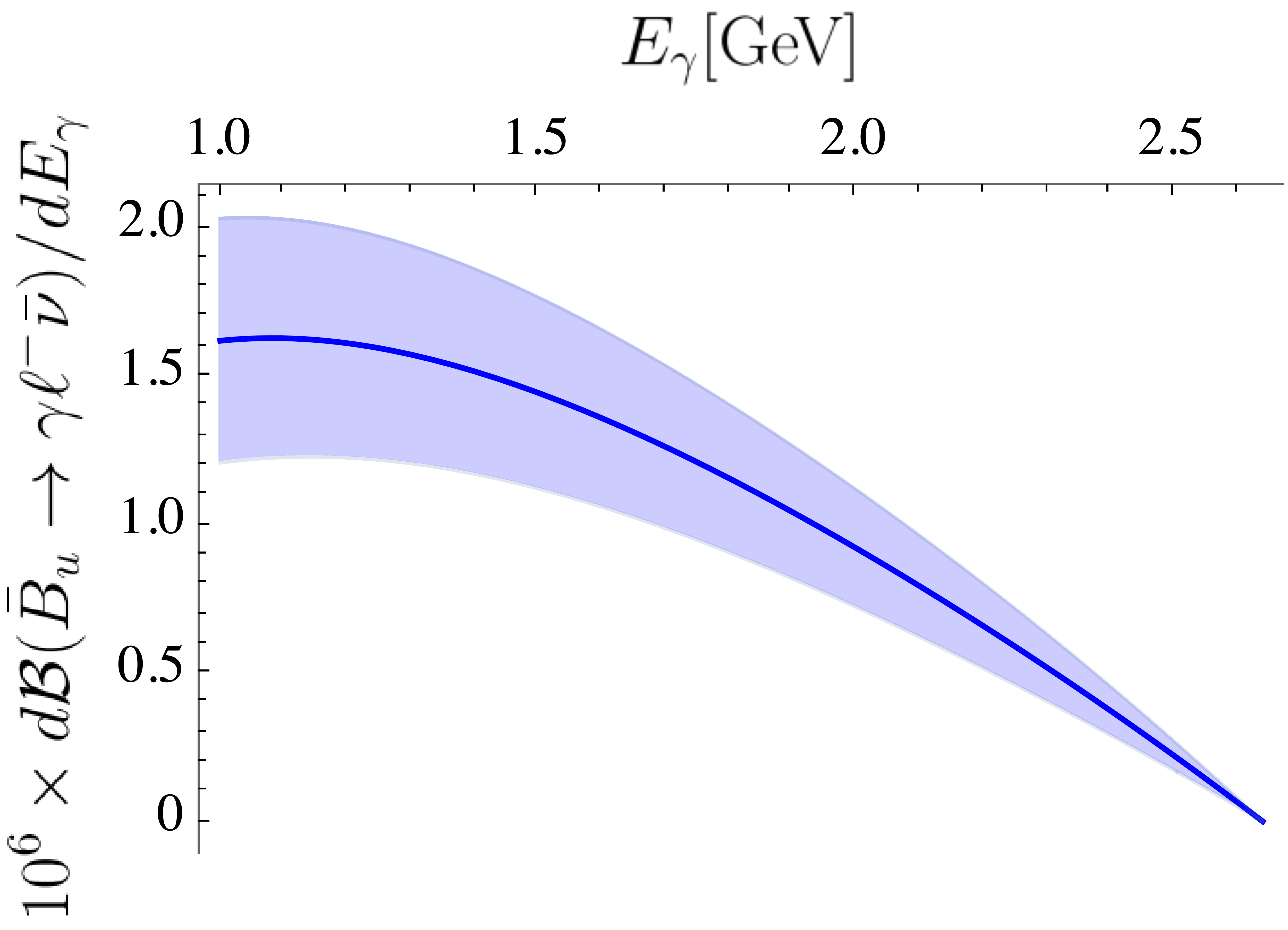
Figure 10: Plots showing the differentiated branching fraction with respect to the di-lepton momentum transfer $q^{2}$ (left) and the photon energy $E_{\gamma}$ (right). The solid blue line indicates the central value with the correlated uncertainty (shaded region) on both the fit-parameters and the CKM matrix element $|V_{\textrm{ub}}|$. The contribution to the total uncertainty from the remaining input parameters is negligible. In the evaluation of the branching ratio we use $G_{F}=1.166378\cdot 10^{-5}\,\mbox{GeV}^{-2}$, $|V_{\textrm{ub}}|=3.82(24)\cdot 10^{-3}$, $\tau_{B}=1.638\cdot 10^{-12}s$ PDG and the fine structure constant at the $B$-meson scale $\alpha=1/129$.

$q^{2}$ bin $[\,\mbox{\small GeV}^{2}]$	$[0,6]\,\mbox{\small GeV}^{2}$	$[2,6]\,\mbox{\small GeV}^{2}$	$[3,6]\,\mbox{\small GeV}^{2}$	$[4,6]\,\mbox{\small GeV}^{2}$
$10^{6}\times\mathcal{B}(\bar{B}_{u}\to\gamma\ell^{-}\bar{\nu})$	0.243(53)	0.214(47)	0.180(39)	0.132(29)
$E_{\gamma}$ bin $[\,\mbox{\small GeV}]$	$[0.5\,\mbox{\small GeV},\frac{m_{B}}{2}]$	$[1.0\,\mbox{\small GeV},\frac{m_{B}}{2}]$	$[1.5\,\mbox{\small GeV},\frac{m_{B}}{2}]$	$[2.0\,\mbox{\small GeV},\frac{m_{B}}{2}]$
$10^{6}\times\mathcal{B}(\bar{B}_{u}\to\gamma\ell^{-}\bar{\nu})$	2.224(554)	1.604(374)	0.883(195)	0.305(67)

Table 7: Integrated branching fraction for various $q^{2}$ and $E_{\gamma}$ bins. The photon energies to the left are denoted by $E_{\gamma}^{\textrm{min}}$ elsewhere in the text. The last three branching fraction predictions are overlaid (rescaled by $(3.70/3.82)^{2}$ since $|V_{\textrm{ub}}|_{\mbox{\cite[cite]{\@@bibref{Authors Phrase1YearPhrase2}{Beneke:2018wjp}{\@@citephrase{(}}{\@@citephrase{)}}} }}=3.70(16)\cdot 10^{-3}$) in Fig. 11 in order to extract $\lambda_{B}$.

5.4 Extraction of the Inverse Moment $\lambda_{B}$ of the $B$-meson DA

As previously mentioned, besides being a toy model for factorisation, $\bar{B}_{u}\to\gamma\ell^{-}\bar{\nu}$ is of interest to extract the $B$-meson DA parameters from experiment. Here, we replace experiment by our computation which comes with the additional bonus that the ${\cal O}(8\%)$ uncertainty of the CKM matrix element $|V_{\textrm{ub}}|=3.82(24)\cdot 10^{-3}$ PDG is eliminated. This is also useful as $|V_{\textrm{ub}}|$ suffers from some tension between exclusive and inclusive $b\to u$ transitions PDG .

Let us turn to some minimal definitions in order to clarify the context. The $B$-meson DA of leading twist-$2$, $\phi^{B}_{+}$ was originally introduced in Grozin:1996pq . Its inverse moment

$$\frac{1}{\lambda_{B}(\mu)}=\int_{0}^{\infty}d\omega\frac{\phi^{B}_{+}(\omega,\mu)}{\omega}\;,$$ (73)

is a genuinely unknown non-perturbative parameter $\lambda_{B}={\cal O}(\Lambda_{\textrm{QCD}})$. Above $\mu$ is the renormalisation scale (or factorisation scale in processes), assumed to be $\mu=1\,\mbox{\small GeV}$ if not stated otherwise. Mainly due to its non-local character it has so far evaded a direct first principle determination. In computations using the heavy quark limit it is often the leading uncertainty. More precisely, at NLO there are two further non-perturbative parameters that appear, the inverse logarithmic moments $\hat{\sigma}_{1,2}$ e.g. DescotesGenon:2002mw ; Beneke:2011nf

$$\hat{\sigma}_{n}(\mu)=\lambda_{B}(\mu)\int_{0}^{\infty}\frac{d\omega}{\omega}\ln^{n}\frac{\mu_{0}}{\omega}\phi_{+}(\omega,\mu)\;,\quad\mu_{0}=\lambda_{B}e^{-\gamma_{E}}\;,$$ (74)

and one should be aware of different conventions due to the choice of $\mu_{0}$ resulting in different values of $\sigma_{n}$. Matters are further complicated by the fact that $\lambda_{B}$ and $\hat{\sigma}_{1,2}$ are defined at $\mu=1\,\mbox{\small GeV}$ but in computations they are evaluated at the hard-collinear scale $\mu={\cal O}(\sqrt{\Lambda_{\textrm{QCD}}m_{b}})\approx 2.2\,\mbox{\small GeV}$. The evolution of the $B$-meson DA parameters involves solving an integro-differential equation Lange:2003ff ; Braun:2019wyx ; Galda:2020epp already at ${\cal O}(\alpha_{s})$ with no autonomous evolution of the parameters (unlike for light-meson DAs where the conformal symmetry allows for a simpler picture, cf. Sec. 4.2.3). In essence a separate (indirect) determination of these parameters is not feasible. Thus actual studies one is forced to use a model-ansatz for $\phi^{B}_{+}$. This is done in reference Beneke:2018wjp for a $3$-parameter family, which permits an analytic evolution at ${\cal O}(\alpha_{s})$. This $3$-parameter model is further constrained to three $2$-parameter models which give rise to the following ranges in $\hat{\sigma}_{1,2}$

Model I $$-0.31<\; \hat{\sigma}_{1} <0.0\;,\quad \phantom{-}0.74<\; \hat{\sigma}_{2} <1.64\;,\quad \textrm{\color[rgb]{0,0,0.5} [blue]}\;,$$

Model II $$-0.31<\; \hat{\sigma}_{1} <0.69\;,\quad \phantom{-}0.74<\; \hat{\sigma}_{2} <5.42\;,\quad \textrm{\color[rgb]{0,0.6,0} [green]}\;,$$

Model III $$-0.69<\; \hat{\sigma}_{1} <0\;,\quad \phantom{-}1.16<\; \hat{\sigma}_{2} <1.64\;,\quad \textrm{\color[rgb]{1,0,0} [red]}\;.$$ (75)

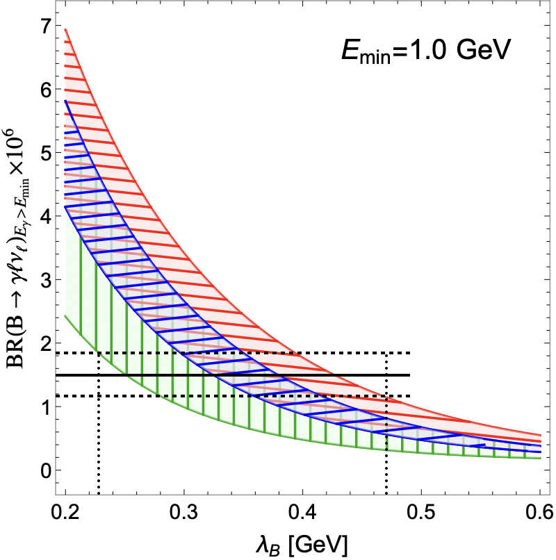
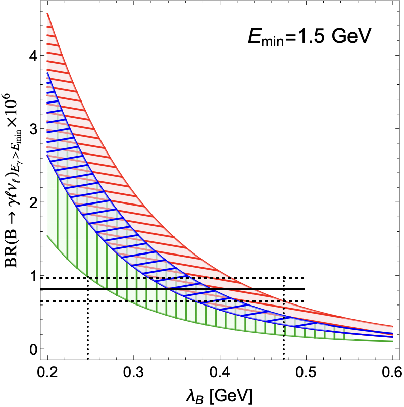
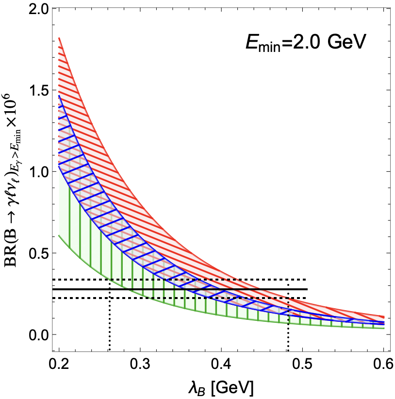
Figure 11: Plots taken from Beneke:2018wjp (coloured curves) overlaid with our predictions for the integrated branching ratios (cf. Tab. 7) scaled to account for the fact that in Beneke:2018wjp $|V_{\textrm{ub}}|_{\textrm{excl}}=3.70(16)\cdot 10^{-3}$ is used. This results an effect of a factor of $0.938$ on the branching fraction. Solid black lines represent our central values with uncertainty bands indicated by dashed lines. The colour coding of the plots corresponds to the different models cf. (5.4) and Beneke:2018wjp of course.

The variation of the model and the model parameter effectively accounts for the lack of knowledge of $\phi^{B}_{+}$.

$E_{\gamma}^{\text{min}}$	$\lambda_{B}^{\text{Model I}}$	$\lambda_{B}^{\text{Model II}}$	$\lambda_{B}^{\text{Model III}}$	$\lambda_{B}^{\text{Model Avg.}}$
$1.0\,\mbox{GeV}$	$355(60)\,\mbox{MeV}$	$295(60)\,\mbox{MeV}$	$415(60)\,\mbox{MeV}$	$350(120)\,\mbox{MeV}$
$1.5\,\mbox{GeV}$	$365(60)\,\mbox{MeV}$	$310(60)\,\mbox{MeV}$	$415(60)\,\mbox{MeV}$	$360(110)\,\mbox{MeV}$
$2.0\,\mbox{GeV}$	$375(60)\,\mbox{MeV}$	$315(60)\,\mbox{MeV}$	$420(60)\,\mbox{MeV}$	$370(110)\,\mbox{MeV}$

Table 8: Values of $\lambda_{B}$ read off from Fig. 11 for the three $\phi_{+}^{B}$ models, rounded to $5\,\mbox{MeV}$. The rightmost column contains the mean value over the models for each minimum photon energy cut, rounded to the nearest $10\,\mbox{MeV}$ and the $E_{\gamma}^{\text{min}}=1.5\,\mbox{GeV}$ is selected as the our final value in (76).

In Fig. 11 we have overlaid our branching fraction predictions, shown in Tab. 7, with the plots from Beneke:2018wjp . From Tab. 8 one sees that the values predicted for a given model are largely stable on the minimum photon energy cut. There is, as expected, some dependence on the specific model of $\phi_{+}^{B}$. However, averaging over the ranges of the three models (cf. right hand column of Tab. 8), one again sees the consistency between the different photon cuts, which suggests good agreement in the shape for these values.

Whereas $E_{\gamma}^{\textrm{min}}=2\,\mbox{\small GeV}$ is arguably the best result because of the range of validity of the approaches, it still seems preferable to take an average of the three values for $\lambda_{B}^{\text{Model Avg.}}$ to deduce our final value in this work

$$\lambda_{B}=360(110){\,\mbox{MeV}}\;.$$ (76)

We now turn to discussing the value obtained in relation to other determinations. The previously mentioned Belle measurement from 2018 sets a bound of $\lambda_{B}>240{\,\mbox{\small MeV}}$ $@90\%\textrm{ CL}$ using Beneke:2018wjp as the reference input. A direct determination via a QCD sum rule, which however uses non-local quark condensates which are not free from model-dependence, was performed in 2003 and gave $\lambda_{B}=460(100){\,\mbox{\small MeV}}$ Braun:2003wx (and the previously quoted value for $\hat{\sigma}_{1}$). An update Khodjamirian:2020hob using improved numerical input and two models for the $B$-meson DA yields $\lambda_{B}=383(153){\,\mbox{\small MeV}}$, a value closer to ours. The same strategy as here has been applied at LO Ball:2003fq ; Khodjamirian:2005ea and NLO Wang:2015vgv ; Gao:2019lta with various specific model functions for $\phi_{+}^{B}$. The $B\to\gamma$ Ball:2003fq LO-analysis has been done in the heavy quark limit and resulting in $\lambda_{B}=600{\,\mbox{\small MeV}}$ with no given error. The LO $B\to\pi$ analysis with an exponential model gave $\lambda_{B}=460(160){\,\mbox{\small MeV}}$ Khodjamirian:2005ea . At NLO there are the works on $B\to\pi$ Wang:2015vgv and $B\to\rho$ Gao:2019lta with $\lambda_{B}=354^{+30}_{-38}{\,\mbox{\small MeV}}$ and $343^{+64}_{-79}{\,\mbox{\small MeV}}$ respectively for which we quote the exponential model values (cf. those references for other model determinations).

$\lambda_{B}[\,\mbox{\small MeV}]$	ref.	year	method	B-DA model
$460(100)$	Braun:2003wx	’03	QCD SR (non-local condensate)	–
$383(153)$	Khodjamirian:2020hob	’20	idem	–
$354^{+30}_{-38}$	Wang:2015vgv	’15	B-LCSR vs LCSR $B\to\pi$ BZ04b ; Duplancic:2008ix	exponential (81) Wang:2015vgv
$368^{+42}_{-32}$	Wang:2015vgv	’15	idem	Model-II (81) Wang:2015vgv
$389^{+35}_{-28}$	Wang:2015vgv	’15	idem	Model-II (81) Wang:2015vgv
$303^{+35}_{-28}$	Wang:2015vgv	’15	idem	Model-II (81) Wang:2015vgv
$343^{+64}_{-79}$	Gao:2019lta	’19	B-LCSR vs LCSR $B\to\rho$ BSZ15	exponential
$370^{+69}_{-86}$	Gao:2019lta	’19	idem	local duality
600	Ball:2003fq	’03	SCET DescotesGenon:2002mw vs LCSR $B\to\gamma$ ($m_{b}\to\infty$)	–
365(60)	this work	’21	LCSR vs SCET Beneke:2018wjp	Model I (5.4a) Beneke:2018wjp
310(60)	this work	’21	idem	Model II (5.4b) Beneke:2018wjp
415(60)	this work	’21	idem	Model III (5.4c) Beneke:2018wjp

Table 9: Comparison-table of $\lambda_{B}$ with respect to the literature. The issue of the model-dependence of the indirect determinations by matching two FF computations is clearly visible. B-LCSR stands for LCSR with a $B$-meson DA. Cf. final paragraph of the section for further comments.

To conclude, from Tab. 9 it is seen that the restriction to a single model does reduce the error considerably and underlines the importance of the QCD SR determinations. In summary, the picture looks consistent but a dedicated heavy quark analysis of the NLO $B\to\gamma$ analysis must ultimately be the most reliable method as it will not involve any photon DAs. We anticipate returning to this issue in a forthcoming publication.

6 Summary and Discussions

In this work we have computed the $\bar{B}_{u,d,s}\to\gamma$ form factors at NLO for twist-$1$,$2$ and LO in twist-$3$,$4$ with light-cone sum rules. This involved the evaluation of the diagrams in Fig. 2 which was the technically most challenging part of this work and involved the use of a series of tools FeynCalc1 ; FeynCalc2 ; litered:2013 ; kira:2017 ; polylogtools and state-of-the-art master integrals DiVita:2017xlr . The form factors are provided as fits to a $z$-expansion ansatz (66) with fit-parameters given in Tab. 4. The correlation matrix can be found in an ancillary file to the arXiv version. Form factor values at $q^{2}=0$ and plots are presented in Tab. 5 and Fig. 7 respectively. This constitutes our main practical results. Analytic results of the correlation functions in terms of Goncharov functions are given as an ancillary file (Mathematica notebook) to the arXiv version. An important technical aside is the choice of the $m_{b}$ mass-scheme for which we have adapted the kinetic scheme, which shows good scale-stability (cf. Fig. 12) unlike the pole- or $\overline{\text{MS}}$-scheme for which either the $\alpha_{s}$- or twist-corrections are unnaturally large.

Besides the form factors themselves, we have established a few valuable theoretical results and advances. In Sec. 2.3, starting from a dispersion representation, we motivated the $m_{b}^{-1/2}$ heavy quark scaling of the $\bar{B}\to\gamma$ form factors from a purely hadronic picture. Additionally, in Sec. 4.2.1, we proposed a scheme to add (strange) quark mass corrections to the magnetic vacuum susceptibility by separating the perturbative part. The following values have been obtained at ${\cal O}(\alpha_{s}^{0})$: $\chi_{q}=3.21(15)\textrm{\small GeV}^{-2}$ and $\chi_{s}=3.79(17)\textrm{\small GeV}^{-2}$. Moreover, the equations of motion (4.4) were verified to hold in all hadronic parameters for which completeness can be expected. In doing so it became clear that in order to include the twist-$4$ $3$-particle distribution amplitude parameters, given in Tab. 12, one needs to include $4$-particle DAs of twist-$4$ which have not yet been classified. For $\bar{B}\to\gamma$ form factors the impact is fortunately rather small.

The charged form factors describe the $\bar{B}_{u}\to\gamma\ell^{-}\bar{\nu}$ decay, anticipated to be measured at Belle II Kou:2018nap , for which our differential rate prediction, binned and including correlation matrix, are given in Sec. 5.3. Comparing to SCET-computations, of three models of the $B$-meson distribution amplitude, we have extracted its inverse moment (73), $\lambda_{B}=360(110)\,\mbox{\small MeV}$. The neutral form factors are the input to the flavour changing neutral current process $\bar{B}_{d,s}\to\gamma\ell^{+}\ell^{-}$, which will come into focus by LHCb in the muon-mode LHCb:2021awg ; LHCb:2021vsc ; LHCbtalk ; Ferreres-Sole:2021qxv , alongside off-shell form factors Albrecht:2019zul and genuine long distance contributions GRZ17 ; Kozachuk:2017mdk ; Beneke:2020fot . The scope of applications of the $\bar{B}\to\gamma$ form factors does not end here as they can serve as inputs, to related processes, in terms of subtraction constants of dispersion relations. Examples are, the weak annihilation process in $\bar{B}\to V\gamma$ e.g. Lyon:2013gba , $B_{s}\to\mu\mu\,\textrm{axion/dark photon}$ for which generic photon off-shell $B\to\gamma^{*}$ form factors are needed (cf. App. A Albrecht:2019zul for how dispersion relations can bridge the $k^{2}\approx m^{2}_{\rho,\omega,\phi}$ resonance region) and $\bar{B}_{u}\to\ell^{+}\ell^{-}\ell^{{}^{\prime}-}\bar{\nu}$ (requiring $q^{2},k^{2}\neq 0$) as recently investigated in Bharucha:2021zay ; Beneke:2021rjf . Our form factor predictions should be helpful in reducing the theory error in all of these modes and enhance the new physics sensitivity.

Acknowledgments

We are grateful to Gunnar Bali, Martin Beneke, Christoph Bobeth, Vladmir Braun, Matteo Di Carlo, Paolo Gambino, Einan Gardi, Yao Ji, Chris Sachrajda and Yuming Wang for useful discussions and to James Gratrex for careful reading of the manuscript. We are indebted to Thomas Gehrmann and Roberto Bonciani for guidance in the master integral literature, Claude Duhr and James Matthews for help with Polylog Tools and Stefano Di Vita, Pierpaolo Mastrolia, Amedeo Primo & Ulrich Schubert for useful exchange and guidance with regard to DiVita:2017xlr . BP is also grateful to Calum Milloy for useful discussions and guidance regarding the method of differential equations and the subtleties therein. RZ acknowledges Damir Becirevic for the kind hospitality at IJCLab, Pôle Théorie Orsay-Paris when this work was in its initial stages. RZ is supported by an STFC Consolidated Grant, ST/P0000630/1. BP is supported by an STFC Training Grant ST/N504051/1.

Ancillary files

We include a number of ancillary files. A file with the renormalised NLO correlation functions for twist-$1$ in terms of MPLs (corr_PT_NLO.m); the new set of master integrals (MI_vzzb.m) discussed in Sec. 4.1.2 which is linearly dependent on the basis DiVita:2017xlr but of value to make cancellations explicit. The $z$-expansion fits, given as a JSON file (BtoGam_FF.json), with some description in Sec. 5.1.2 and the notebook (FF-plots_from_json.nb) that exemplifies its implementation.

Appendix A Conventions and Additional Plots

We define the covariant derivative as

$$D_{\mu}=\partial_{\mu}+s_{e}ieQ_{f}A_{\mu}+s_{g}ig_{s}A^{a}_{\mu}T^{a}$$ (A.1)

where $e>0$ ($\alpha=e^{2}/(4\pi))$, $Q_{e}=-1$, $Q_{u,c,t}=2/3$ and $Q_{b,d,s}=-1/3$. This leads to a Feynman rule $-s_{e}ieQ_{f}\not{A}-s_{g}ig_{s}\not{A^{a}}T^{a}$. Note that the sign of the FFs (2.1) depends on $s_{e}$ which we therefore prefer to keep explicit. The sign of the gluon term $s_{g}$ is also kept which appears in the light-cone propagator in the background field (D.3) as well as the $3$-particle DAs. The final results are independent of $s_{g}$ and the rate is of course independent of $s_{e}$, but attention must be paid when compared or combined with other work. Using the $g=\textrm{diag}(1,-1,-1,-1)$ metric the following relation holds,

$$\sigma^{\alpha\beta}\gamma_{5}=-\frac{i}{2}\varepsilon^{\alpha\beta\gamma\delta}\sigma_{\gamma\delta}\;,$$ (A.2)

with $\varepsilon_{0123}=1$ and $\gamma_{5}=i\gamma^{0}\gamma^{1}\gamma^{2}\gamma^{3}$. Moreover we have $T^{a}T^{a}=C_{F}\mathbf{1}$ with $C_{F}=(N_{c}^{2}-1)/(2N_{c})$ and $\alpha_{s}=g^{2}/(4\pi)$ as usual.

A.1 Borel Transformation

The Borel transform is defined as

$$f_{\hat{\mathcal{B}}}(M_{\hat{\mathcal{B}}}^{2})={\hat{\mathcal{B}}}f(Q^{2})=\lim_{Q^{2}\to\infty,n\to\infty}\dfrac{(Q^{2})^{n+1}}{n!}\left(-\dfrac{d}{dQ^{2}}\right)^{n+1}f(Q^{2})$$ (A.3)

where $Q^{2}=-q^{2}$ is a Euclidean momentum and $Q^{2}/n=M_{\hat{\mathcal{B}}}^{2}$ defines the so-called Borel mass.

For the perturbative part and the condensates, which are poles at tree level, one needs the following Borel transformation

$${\hat{\mathcal{B}}}\dfrac{1}{(Q^{2}+m^{2})^{a}} =\dfrac{1}{\Gamma(a)(M_{\hat{\mathcal{B}}}^{2})^{a}}e^{-m^{2}/M_{\hat{\mathcal{B}}}^{2}}\,.$$ (A.4)

The DA-part can be reduced to a form $du\frac{1}{\Delta^{n}}$ ($n\geq 1$) for which simple rules for Borel transformation are given in App. A in BSZ15 . Of course one could integrate over the DA-parameters $du$ or $D\underline{\alpha}$, then subject the result to a dispersion relation and use (A.4). The advantage of using the former method is that one does not need to commit to a specific form/truncation of the DAs.

A.2 Plots of Scale Dependence and Twist-contributions

In this appendix we collect additional plots and tables.

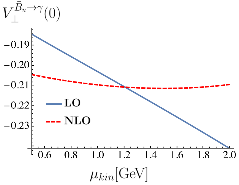
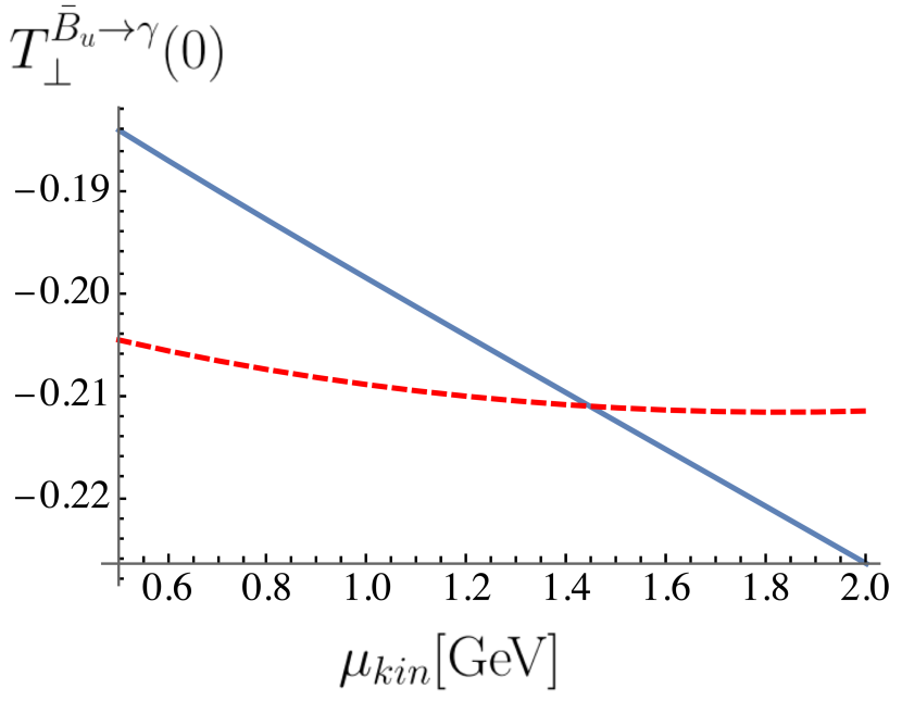
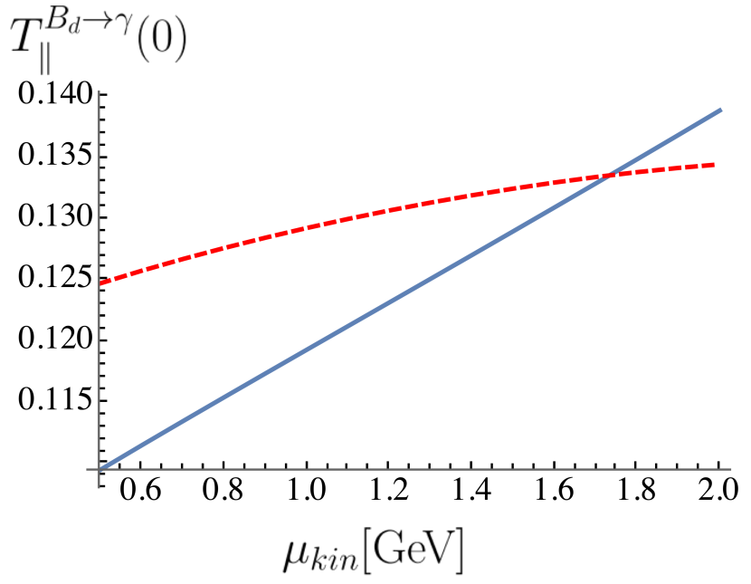
Figure 12: Plots of a representative selection of form factors, evaluated at $q^{2}=0$. The plots serve to highlight the reduction in the kinetic scale dependence when radiative corrections to twist-1 and -2 are included (dashed red line) as compared to the LO result (solid blue line).

The merit of the NLO versus a LO analysis shows in the mass scale dependence plots in Fig. 12. The advantages of the kinetic-scheme over the pole- and $\overline{\text{MS}}$- schemes become apparent in Fig. 13 and Tab. 10, respectively.

twist	DA	$V_{\|}^{\bar{B}_{u}\to\gamma}(0)$		$V_{\perp}^{\bar{B}_{d}\to\gamma}(0)$		$T_{\perp,\|}^{\bar{B}_{u}\to\gamma}(0)$
		Kin	$\overline{\text{MS}}$	Kin	$\overline{\text{MS}}$	Kin	$\overline{\text{MS}}$
1	$\textrm{PT}\,{\cal O}{(\alpha_{s}^{0})}$	$45.7\%$	$70.0\%$	$51.3\%$	$86.2\%$	$51.4\%$	$79.5\%$
1	$\textrm{PT}\,{\cal O}{(\alpha_{s})}$	$8.4\%$	$-6.3\%$	$14.9\%$	$-18.0\%$	$16.5\%$	$-10.6\%$
2	$\phi_{\gamma}(u)\,{\cal O}{(\alpha_{s}^{0})}$	$62.3\%$	$119.1\%$	$28.5\%$	$47.2\%$	$24.4\%$	$35.8\%$
2	$\phi_{\gamma}(u)\,{\cal O}{(\alpha_{s})}$	$9.5\%$	$-38.7\%$	$4.1\%$	$-16.8\%$	$4.3\%$	$-8.7\%$
3	$\Psi_{(a)}(u)$	–	–	$0.6\%$	$-0.1\%$	$0.5\%$	$0.2\%$
3	$\Psi_{(v)}^{(1)}(u)$	$2.5\%$	$3.7\%$	–	–	$0.8\%$	$0.9\%$
4	$h_{\gamma}^{(2)}(u)$	$-9.2\%$	$-15.3\%$	–	–	$-1.6\%$	$-1.9\%$
4	$\mathbb{A}(u)$	$-12.1\%$	$-20.2\%$	$-5.9\%$	$-8.5\%$	$-4.2\%$	$-5.1\%$
4	$Q_{q}\left\langle\bar{q}q\right\rangle$	$-8.8\%$	$14.5\%$	–	–	–	–
4	$Q_{b}\left\langle\bar{q}q\right\rangle$	$-2.9\%$	$-4.9\%$	$2.8\%$	$4.2\%$	$2.4\%$	$3.1\%$
	Total∗	$-0.118$	$-0.097$	$0.127$	$0.125$	$0.127$	$0.130$

Table 10: A comparison of the different twist contributions in the kinetic and $\overline{\text{MS}}$ schemes (with $\mu_{\textrm{kin}}=1\,\mbox{GeV}$ and $\mu_{\overline{\text{MS}}}=m_{b}(m_{b})=4.18\,\mbox{GeV}$) for a selection of illustrative form factors. Columns represent the percentage contribution of each DA to “Total^∗”. We remind the reader that the asterisk in total indicates it includes twist-$4$ contributions that do not close under the EOM (cf. Sec. 4.4). Contributions from 3-particle DAs have been dropped for brevity. Formally one should redetermine the sum rule parameters (cf. Tab. 2) for the $\overline{\text{MS}}$ evaluation, however we choose to use the same parameters as for the kinetic evaluation as this is sufficient to illustrate our point. We note the kinetic scheme shows greater suppression of the higher twist contributions. Additionally, in contrast to the kinetic scheme, radiative corrections in the $\overline{\text{MS}}$-scheme act to cancel with the LO results.

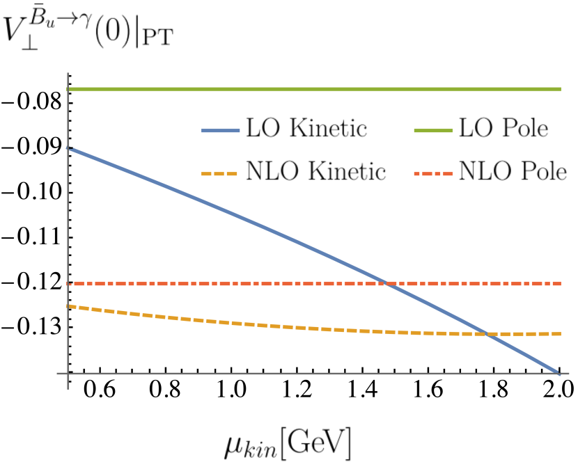
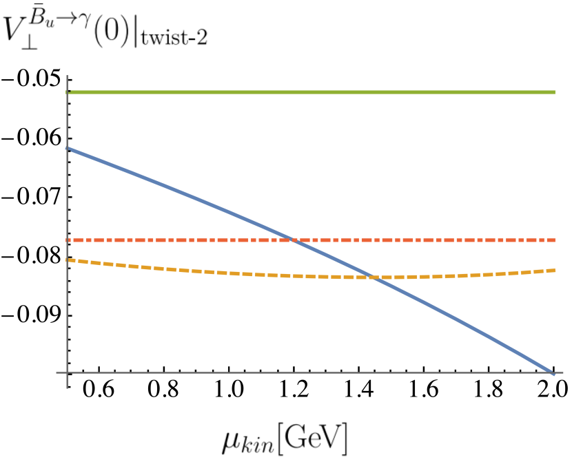
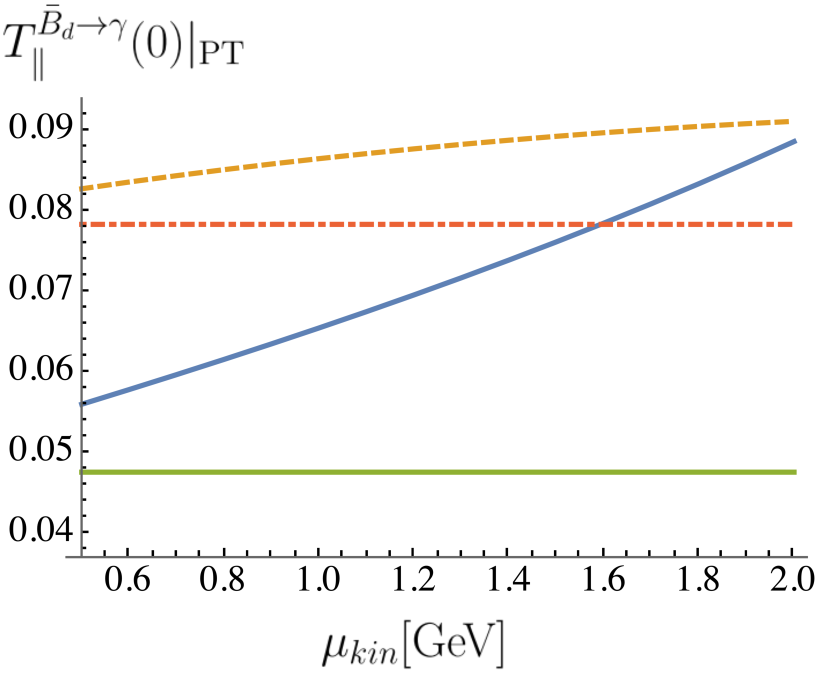
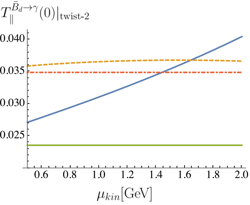
Figure 13: Plots comparing the relative size of the radiative corrections to twist-$1$ and -$2$ in the pole- and kinetic-scheme, for two representative form factors. We observe large corrections in the pole scheme, with the ${\cal O}(\alpha_{s})$ contributions being in the region of $50$-$60\%$ and $40$-$50\%$ of the LO result at twist-1 and -2, respectively. In contrast, using the kinetic scheme at $\mu_{\textrm{kin}}=1\,\mbox{GeV}$, we find the NLO corrections are approximately $\sim 20\%$ and $\sim 10\%$ of the LO result at twist-1 and -2, respectively.

Appendix B Gauge (In)variance and the $m_{\ell}=0$ Amplitude

In this appendix we intend to clarify a few issues around gauge invariance.

B.1 Gauge-variant part of the Charged Form Factor

In Sec. 3.2 it was shown how the $Q_{\bar{B}}$-term in (2.1) appears in the LCSR computation and below its consistency is illustrated on general grounds. The $Q_{\bar{B}}$-term is present since $O_{\mu}$ itself is not gauge invariant (charged) in the case where the weak current is charged. Let us write the matrix element on the LHS of (2.1) as follows

$$\langle\gamma(k,\epsilon)|O^{V}_{\mu}|\bar{B}_{q}(p_{B})\rangle=-i\epsilon^{*}_{\rho}\int_{y}e^{ik\cdot y}\langle 0|Tj^{\rho}(y)O^{V}_{\mu}(0)|\bar{B}_{q}(p_{B})\rangle+\textrm{gauge-invariant}\;,$$ (B.1)

and then perform a gauge tranformation $\epsilon\to\epsilon+k$,

$$-ik_{\rho}\int_{y}e^{ik\cdot y}\langle 0|Tj^{\rho}(y)O^{V}_{\mu}(0)|\bar{B}_{q}(p_{B})\rangle \;=\; e\langle 0|[Q,O^{V}_{\mu}(0)]|\bar{B}_{q}\rangle$$ (B.2)

$$\;=\; Q_{\bar{B}}m_{B}\langle 0|\bar{q}\gamma_{\mu}(1-\gamma_{5})b|\bar{B}_{q}\rangle=-iQ_{\bar{B}}m_{B}(p_{B})_{\mu}f_{B}\;,$$

where we have used $\{q_{\alpha}^{\dagger}(\vec{x},0),q_{\beta}(0)\}=\delta^{(3)}(\vec{x})\delta_{\alpha\beta}$. It is readily seen that this matches the gauge variation of the Low-term on the RHS in (2.1).

B.2 Gauge Invariance Restored, in the $\bar{B}_{u}\to\gamma\ell^{-}\bar{\nu}$-Amplitude

Here we illustrate that the total amplitude, emission from the $B$-meson (i.e. FF) and the lepton leg, is gauge invariant. The total amplitude ${\cal A}$ is proportional to

$${\cal A}[\bar{B}_{u}\to\ell^{-}\bar{\nu}\gamma(\epsilon)]\propto e\epsilon^{*}_{\rho}\int_{y}e^{iky}\left(\langle 0|Tj^{\rho}(y)O_{\mu}^{V}|\bar{B}_{u}\rangle\langle\ell^{-}\bar{\nu}|L^{\mu}|0\rangle+\langle 0|O_{\mu}^{V}|\bar{B}_{u}\rangle\langle\ell^{-}\bar{\nu}|Tj^{\rho}(y)L^{\mu}|0\rangle\right)\;,$$

where $H^{\textrm{eff}}\sim L^{\mu}O^{V}_{\mu}$ and $L^{\mu}=\bar{\ell}\Gamma^{\mu}\nu$ is the charged lepton current with some unspecified Dirac matrix $\Gamma^{\mu}$. The total amplitude must be invariant under the residual gauge transformation $\epsilon\to\epsilon+k$,

$$\delta_{\textrm{gauge}}{\cal A} \;\equiv\; {\cal A}(\bar{B}_{u}\to\ell^{-}\bar{\nu}\gamma(\epsilon+k))-{\cal A}(\bar{B}_{u}\to\ell^{-}\bar{\nu}\gamma(\epsilon))$$

$$\;\propto\; ie\underbrace{(Q_{b}-Q_{u}-Q_{\ell})}_{=0}\langle 0|O_{\mu}^{V}|\bar{B}_{u}\rangle\langle\ell^{-}\bar{\nu}|L^{\mu}|0\rangle=0\;,$$ (B.3)

which is the case if charge conservation is imposed ($Q_{b}=-1/3$, $Q_{u}=2/3$ and $Q_{\ell}=-1$). In conclusion, the total amplitude is indeed invariant under $\epsilon\to\epsilon+k$.

B.3 The $\bar{B}_{u}\to\gamma\ell^{-}\bar{\nu}$-Amplitude at $m_{\ell}\to 0$

The $m_{\ell}$-case is special in that the emission term is local and allows a redefinition of the FF to absorb all effects Beneke:2011nf . We follow this procedure in our notation as we consider it worthwhile to make contact with the existing literature.

• In the $m_{\ell}=0$ case the emission from the lepton is proportional to the tree level matrix element. Essentially

  $$\epsilon^{*}_{\rho}\langle\ell(l_{1})\nu(l_{2})|\bar{\ell}\not{p}_{B}\frac{\not{k}+\not{l_{1}}}{(k+l_{1})^{2}}\gamma^{\rho}\nu|0\rangle=\epsilon^{*}_{\rho}\langle\ell(l_{1})\nu(l_{2})|\bar{\ell}\gamma^{\rho}\nu|0\rangle\;,$$ (B.4)

  where $p_{B}=k+l_{1}+l_{2}$ and the EOM was used for the $\nu$. This allows to redefine the FF in such a way that the amplitude is proportional to the FF only.

• Focusing on the $\gamma_{5}$-part of the FFs (2.1)

  $$\langle\gamma(k,\epsilon)|O^{V}_{\mu}|\bar{B}_{q}(p_{B})\rangle|_{\gamma_{5}-\textrm{part}} \;=\; s_{e}\left(-P^{\parallel}_{\mu}\left(V_{\parallel}(q^{2})+Q_{\bar{B}}\frac{m_{B}f_{B}}{k\cdot p_{B}}\right)-(p_{B})_{\mu}im_{B}Q_{\bar{B}}\frac{\epsilon^{*}\cdot p_{B}}{k\cdot p_{B}}f_{B_{q}}\right)$$

  $$\;=\; s_{e}(-P^{\parallel}_{\mu}\,V_{\parallel}(q^{2})+i\epsilon^{*}_{\mu}m_{B}f_{B}Q_{\bar{B}}+{\cal O}(q_{\mu}))\;,$$ (B.5)

  where the ${\cal O}(q_{\mu})$ terms are irrelevant as they vanish in the massless case when contracted with the vector or axial lepton matrix element.

• By gauge invariance of the full amplitude, as argued above, it is then clear that the extra $\epsilon_{\mu}^{*}$-term must cancel the emission term and thus the full amplitude can be written as

  $${\cal A}[\bar{B}_{u}\to\ell^{-}\bar{\nu}\gamma(\epsilon)]\big{|}_{m_{\ell}=0}\propto s_{e}\big{(}P^{\perp}_{\mu}\,V_{\perp}(q^{2})-P^{\parallel}_{\mu}\,V_{\parallel}(q^{2})\big{)}\,\langle\ell(l_{1})\bar{\nu}(l_{2})|\bar{\ell}\Gamma^{\mu}\nu|0\rangle\;.$$ (B.6)

  It seems worthwhile to comment on why in the $m_{\ell}=0$ approximation the point-like structure (terms proportional to $f_{B}$ (2)) disappears. This is the case since the point-like term is given by the LO matrix element times $\epsilon^{*}\cdot p_{B}$ and other factors. This is a consequence of Low’s theorem Low:1958sn and means that as far as angular momentum conservation is concerned it behaves like the LO matrix element. The additional photon forms a Lorentz scalar with $p_{B}$ and is thus in a relative $p$-wave to the $B$-meson. Finally, since the LO matrix element is helicity suppressed (proportional to $m_{\ell}$) this contribution vanishes entirely in the $m_{\ell}\to 0$ limit.

Appendix C Correlation Functions and Equations of Motion

In this appendix we wish to clarify a few technical aspects regarding the EOM.

C.1 Derivation of the Equations of Motion at Correlation Function Level

To what extent the naive EOM

$$\bar{q}i(D^{\nu}i\sigma_{\mu\nu}+\overset{\leftrightarrow}{D}_{\mu})[\gamma_{5}]b+(m_{q}\pm m_{b})\bar{q}\gamma_{\mu}[\gamma_{5}]b=0\;,$$ (C.1)

($A\stackrel{{\scriptstyle\leftrightarrow}}{{\partial}}_{\mu}B\equiv({\partial}_{\mu}A)B-A({\partial}_{\mu}B)$) are altered in correlation functions by CTs is a typical field theory problem. Below we give the correlation function version of (C.1) with insertion of the photon and $B$-meson currents. The main result is that with the definition of $\Pi_{\parallel}$, compatible with the QED WI, the EOM are satisfied in the most straightforward way

$$\Pi^{T}_{\perp}(p_{B}^{2},q^{2})+\Pi^{\cal D}_{\perp}(p_{B}^{2},q^{2}) \;=\; \frac{(m_{b}+m_{q})}{m_{B}}\Pi^{\cal V}_{\perp}(p_{B}^{2},q^{2})\;,$$

$$\Pi^{T}_{\parallel}(p_{B}^{2},q^{2})+\Pi^{\cal D}_{\parallel}(p_{B}^{2},q^{2}) \;=\; \frac{(m_{b}-m_{q})}{m_{B_{q}}}\Pi^{\cal V}_{\parallel}(p_{B}^{2},q^{2})\;.$$ (C.2)

This equation is the basis for the simple relation (4.4) and the usual statement in the literature that the EOM hold on physics states. Below we show how (C.1) emerges, despite a few CTs on the way, by starting with correlation functions in coordinate space.

C.1.1 Current Insertion (hard Photon)

By variation from the path integral under $q(x)\to\epsilon_{q}(x)$ and $\bar{b}(x)\to\bar{\epsilon}_{b}(x)$ and requiring independence in $\epsilon_{q}(x)$ and $\epsilon_{b}(x)$ one gets two equations which can be combined to

$$\langle 0|T\bar{q}i(\overset{\leftarrow}{\not{D}}\gamma_{\mu}[\gamma_{5}]\mp\gamma_{\mu}[\gamma_{5}]\overset{\rightarrow}{\not{D}})b(x)j_{B}(y)j_{\rho}(0)|0\rangle = -(m_{q}\pm m_{b})\langle 0|T\bar{q}\gamma_{\mu}[\gamma_{5}]b(x)j_{B}(y)j_{\rho}(0)|0\rangle$$ (C.3)

$$-i\delta(x-0)\,g_{\mu\rho}\overline{Q}\langle 0|Tj_{B}(y)j_{\tilde{B}[B]}(0)|0\rangle$$

$$+i\delta(x-y)\,\langle 0|TA[V]_{\mu}(y)j_{\rho}(0)|0\rangle\;,$$

where $\overline{Q}\equiv(Q_{b}+Q_{q})$, $j_{\tilde{B}[B]}\equiv\bar{b}[\gamma_{5}]q$ and $V[A]_{\mu}=\sum_{f=q,b}\bar{f}\gamma_{\mu}[\gamma_{5}]f$. By using the identity

$$iD^{\nu}\bar{q}i\sigma_{\mu\nu}[\gamma_{5}]b=-i\bar{q}\overset{\leftrightarrow}{D}_{\mu}[\gamma_{5}]b+\bar{q}(i\overset{\leftarrow}{\not{D}}\gamma_{\mu}[\gamma_{5}]\mp\gamma_{\mu}[\gamma_{5}]i\overset{\rightarrow}{\not{D}})b\;,$$ (C.4)

one gets the useful forms for the $\perp$-direction

$$\langle 0|T\bar{q}i(D^{\nu}i\sigma_{\mu\nu}+\overset{\leftrightarrow}{D}_{\mu})b(x)j_{B}(y)j_{\rho}(0)|0\rangle+(m_{q}+m_{b})\langle 0|T\bar{q}\gamma_{\mu}b(x)j_{B}(y)j_{\rho}(0)|0\rangle=0\;,$$ (C.5)

and the $\parallel$-direction

$$\langle 0|T\bar{q}i(D^{\nu}i\sigma_{\mu\nu}+\overset{\leftrightarrow}{D}_{\mu})\gamma_{5}b(x)j_{B}(y)j_{\rho}(0)|0\rangle+(m_{q}-m_{b})\langle 0|T\bar{q}\gamma_{\mu}\gamma_{5}b(x)j_{B}(y)j_{\rho}(0)|0\rangle=$$

$$-i\delta(x-0)\,g_{\mu\rho}\overline{Q}\langle 0|Tj_{B}(y)j_{B}(0)|0\rangle+i\delta(x-y)\,\langle 0|TV_{\mu}(y)j_{\rho}(0)|0\rangle\;.$$ (C.6)

Above all derivatives are understood as being outside the timer-ordered products. This leads to particularly simple rules in momentum space. In order to make contact with our previous discussion we take the Fourier transformation $\int_{x}e^{iqx}\int_{y}e^{-ip_{B}y}$. All CTs are absent for the $\perp$-direction, while for the $\parallel$-direction the $\delta(x-0)$- and the $\delta(x-y)$-terms lead to correlation functions in the variables $p_{B}^{2}$ and $k^{2}$ respectively. Crucially, when contracting with the photon polarisation tensor $\epsilon^{*\rho}$ these terms are proportional to $\epsilon^{*\mu}$ and thus do not contribute to our projection prescription (28). Hence for the current insertion the EOM do indeed assume the simplest possible form (C.1).

C.1.2 Distribution Amplitude Part (soft Photon)

If the photon is not created by the perturbative current then the analogues of (C.5) and (C.1.1) are given by

$$\langle\gamma|T\bar{q}i(\partial^{\nu}i\sigma_{\mu\nu}+\overset{\leftrightarrow}{D}_{\mu})[\gamma_{5}]b(x)j_{B}(y)|0\rangle+(m_{q}\pm m_{b})\langle\gamma|T\bar{q}\gamma_{\mu}[\gamma_{5}]b(x)j_{B}(y)|0\rangle=$$ (C.7)

$$+i\delta(x-y)\,\underbrace{\langle\gamma|A[V]_{\mu}(y)|0\rangle}_{=0}\;,$$

where ${\langle\gamma|A_{\mu}(y)|0\rangle}=0$ by parity and ${\langle\gamma|V_{\mu}(y)|0\rangle}=0$ when the photon is not point-like, as is the case here. Not surprisingly the EOM assume the same simple form (C.1) as the current insertion contributions.

C.2 Renormalisation of Correlation Functions and Equation of Motion

Since the (non)renormalisation of the EOM has only been briefly discussed in BSZ15 and involves some mixing of operators we consider it worthwhile to revisit this matter, thereby showing the consistency of our results with the computation of the renormalisation matrix BSZ15 .

In order to clarify the notation we remind the reader of the renormalisation of a Wilson coefficient in the OPE. The Wilson coefficients correspond, after Fourier transformation, to the hard scattering kernels $T_{H}$ in the notation in (39). We may discuss the renormalisation in the language of the local OPE.

We use the notation $O_{i}^{(0)}=\bar{Z}_{ij}O_{j}=Z_{q}Z_{ij}O_{j}$ to denote the relation between bare and renormalised operators. The bare renormalisation constants include the wavefunction renormalisation $Z_{q}$. The local OPE is parameterised by $\langle O_{A}(x)O_{B}(0)\rangle_{\varphi}=C^{C}_{AB}(x)\langle O_{C}(0)\rangle_{\varphi}$ where $\langle\dots\rangle_{\varphi}$ denotes a matrix element over physical states and summation over the index $C$ is understood. The OPE equation may be written as

$$(\bar{Z}^{-1})_{AA^{\prime}}(\bar{Z}^{-1})_{BB^{\prime}}\langle O^{(0)}_{A^{\prime}}(x)O^{(0)}_{B^{\prime}}(0)\rangle_{\varphi}=C^{C}_{AB}(x)\langle O_{C}(0)\rangle_{\varphi}\;,$$ (C.8)

where it was used that the renormalisation matrix of the Wilson coefficient and the operator are each other’s inverse. This is valid in mass-independent schemes such as DR with $\overline{\text{MS}}$.

In our case: (i) $O_{B}\to J_{B_{q}}$ which does not renormalise and thus $\bar{Z}_{BB^{\prime}}\to 1$ in the formula above, (ii) $O_{C}\to O_{T}\sim\bar{q}\sigma_{\mu\nu}q$ which renormalises multiplicatively, and we use $Z_{T}=\bar{Z}_{TT}=Z_{q}Z_{TT}$, (iii) $O_{B}\to O^{D}$ for which the renormalisation is more involved BSZ15 . We may simplify the task by absorbing the operator $O_{4}$ in BSZ15 , $(O_{1})|_{\textrm{here}}=(O_{1}-O_{4})|_{\!\!\mbox{\small{\cite[cite]{\@@bibref{Authors Phrase1YearPhrase2}{BSZ15}{\@@citephrase{(}}{\@@citephrase{)}}}}}}$,

$$O_{1}=O_{D}=2\bar{q}i\!\stackrel{{\scriptstyle\leftarrow}}{{D}}_{\mu}-i\partial_{\mu}(\bar{q}b)=\bar{q}i\!\stackrel{{\scriptstyle\leftrightarrow}}{{D}}_{\mu}b\;,\quad\;,$$

$$O_{2}=O_{\partial T}=i\partial^{\nu}(\bar{q}i\sigma_{\mu\nu}b)\;,\quad O_{3}=O_{mV}=(m_{q}+m_{b})\bar{q}\gamma_{\mu}b\;,$$ (C.9)

for which the renormalisation matrix, computed in BSZ15 cf. App. A, reads

$$Z_{AA^{\prime}}=\delta_{AA^{\prime}}+\Delta\left(\begin{matrix}2&2&6\\ 0&0&0\\ 0&0&(2-6)\end{matrix}\right)\;,\quad\bar{Z}_{AA^{\prime}}=\delta_{AA^{\prime}}+\Delta\left(\begin{matrix}0&2&6\\ 0&-2&0\\ 0&0&-6\end{matrix}\right)\;.$$ (C.10)

Above and hereafter

$$\Delta=C_{F}\frac{\alpha_{s}}{4\pi}\frac{1}{4-d}=C_{F}\frac{\alpha_{s}}{4\pi}\frac{1}{2\epsilon_{\textrm{UV}}}\;,$$ (C.11)

and $Z_{q}=1-2\Delta$ (Feynman gauge) was used to translate from $Z_{AA^{\prime}}$ to $\bar{Z}_{AA^{\prime}}$. In this basis the non-renormalisation of the EOM,

$$\langle(O^{(0)}_{\partial T}+O^{(0)}_{D}+O^{(0)}_{mV})\dots\rangle_{\varphi}=\langle(O_{\partial T}+O_{D}+O_{mV})\dots\rangle_{\varphi}\;,$$ (C.12)

is expressed by the columns of $\bar{Z}_{AA^{\prime}}$ adding up to zero. Above the dots stand for single insertion of fields leading to CTs on the LHS. If the field insertions are absent the EOM simply assume the form $\langle(O^{(0)}_{\partial T}+O^{(0)}_{D}+O^{(0)}_{mV})\rangle_{\varphi}=\langle(O_{\partial T}+O_{D}+O_{mV})\rangle_{\varphi}=0$.

In summary, dropping the index $B$, (C.8) simplifies to

$$C^{T}_{A}(x)\langle O_{T}(0)\rangle_{\varphi}=(\bar{Z}^{-1})_{AA^{\prime}}\langle O^{(0)}_{A^{\prime}}(x)J_{B_{q}}^{(0)}(0)\rangle_{\varphi}\;.$$ (C.13)

After this general discussion it remains to adapt to the operator basis used in this paper. The relation is as follows

$$O^{V}=-\frac{1}{e}\frac{m_{B}}{(m_{b}+m_{q})}O_{mV}\;,\quad O^{T,D}=\frac{1}{e}O_{\partial T,D}\;.$$ (C.14)

In the basis (C.14), in which our correlation function are presented, the UV-counterterms assume the form

$$\delta\Pi^{D}=\Delta\left(-2\Pi^{T(0)}+6\frac{m_{b}+m_{q}}{m_{B}}\Pi^{V(0)}\right)\;,\quad\delta\Pi^{T}=2\Delta\Pi^{T(0)}\;,\quad\delta\Pi^{V}=0\;,$$ (C.15)

taking into account that the $O_{V}$-$O_{mV}$ relation (C.14) implies a sign flip $\bar{Z}_{13^{\prime}}$ and dropping $+6$ in $\bar{Z}_{33}$ (it corresponds to the mass renormalisation $Z_{m}=1-6\Delta$). Concluding, we have explicitly checked that the renormalised $\Pi^{\Gamma}$ quantity

$$\Pi^{\Gamma}|_{\textrm{NLO}}\equiv\Pi^{\Gamma(0)}+\Pi^{\Gamma(1)}+\delta\Pi^{\Gamma}|_{m_{b}\to Z_{m}m_{b}}\;,$$ (C.16)

is free from UV-divergencies when expanded to order ${\cal O}(\alpha_{s})$. Above the superscripts $(0)$ and $(1)$ stand for LO and NLO respectively. We have explicitly verified (C.16) in our NLO computations, that is twist-$1$ and twist-$2$. As usual this shows consistency of the explicit computation and that $Z_{AA^{\prime}}$ is implicitly contained in the computation of this paper.

Appendix D Compendium for the Photon Distribution Amplitude

In this appendix we collect the information on the photon DAs. The main paper on the photon DA is Ball:2002ps where the powerful background field technique is used. The photon DA was originally introduced in Balitsky:1997wi . The reasons for writing such an appendix are at least threefold. First we collect the DAs used in this paper in more a compact way, second we include quark mass corrections and thirdly the DAs are presented in a format which is more useful for computations (e.g. elimination of $1/kz$-factors through integration by parts and replacing $\epsilon^{\perp}$ etc by standard vectors). The most sizeable quark mass corrections are due to twist-$2$, the correction to the magnetic vacuum susceptibility Sec. 4.2.1 ,and the mixing into the twist-$3$ DA via the EOM.

In reference Ball:2002ps the photon DA are given for an external photon field (i.e. $\langle 0|\dots|0\rangle_{F_{\mu\nu}}$) as well as for a single photon state (i.e. $\langle\gamma(q,\epsilon)|\dots|0\rangle$). The two are related by assuming a plane wave for the external field. In this appendix we use the latter. The photon DAs and their hadronic parameters are defined in Secs. D.1 and D.2 respectively. A small dictionary between DAs of the photon and vector mesons is given in Tab. 11. The light-cone propagator in the background gauge field is given in the Sec. D.3 and which tangentially fits into this appendix.

D.1 Matrix Elements of the Photon Distribution Amplitude

The photon DAs are largely analogous to the vector meson ones, cf. Tab. 11. We identify two main differences. Since the photon is massless, the pure $m_{V}$-terms are zero and $\langle\gamma|\bar{q}F_{\mu\nu}q|0\rangle$ matrix elements play a distinguished role as they do not introduce new hadronic parameters.

It is convenient to first introduce $\epsilon^{\perp}$ and $g^{\perp}_{\mu\nu}$ BBKT98

$$g_{\perp}^{\mu\nu}=g^{\mu\nu}-\frac{1}{kz}(k^{\mu}z^{\nu}+k^{\nu}z^{\mu})\;,\quad\epsilon^{\perp}=\epsilon-\frac{\epsilon z}{kz}k-\frac{\epsilon k}{kz}z=\epsilon-\frac{\epsilon z}{kz}k\;,$$ (D.1)

which are orthogonal to the light-like directions $z$ and $k$ (photon momentum): $\epsilon^{\perp}k=\epsilon^{\perp}z=0$ and $(g^{\perp}q)_{\mu}=(g^{\perp}z)_{\mu}=0$. It is also worth noting that $\epsilon^{\perp}$ is invariant under $\epsilon\to\epsilon+k$ which is the residual gauge transformation of the Lorenz gauge $\epsilon(k)\cdot k=0$. In the formulae we use $g_{\mu\nu}$ and $\epsilon_{\mu}$ rather than the $\perp$ version. Factors $1/kz$ that arise from these quantities are treated, as usual, via integration by parts

$$\frac{1}{kz}\int_{0}^{1}\!\!du\,e^{i\bar{u}[u]kz}f(u)\to i[-i]\!\int_{0}^{1}\!\!du\,e^{i\bar{u}kz}I_{1}[f](u),\quad I_{1}[f](u)\ =\ \int_{0}^{u}\!\!dv\,f(v),$$ (D.2)

where $\int_{0}^{1}dvf(v)=0$ is assumed and has to hold in order to produce a smooth $kz\to 0$ limit. More concretely, we use the notation

$$F^{(1)}(u) \;\equiv\; I_{1}[F](u)=\int_{0}^{u}dw\,F(w)\;,$$

$$F^{(2)}(u) \;\equiv\; I_{2}[F](u)=I_{1}\circ I_{1}[F](u)=\int_{0}^{u}dw\int_{0}^{w}dv\,F(v)\;.$$ (D.3)

When comparing with Ball:2002ps it should be taken into account that these authors use $s_{e}|_{\textrm{BBK}}=-1$ and $s_{g}|_{\textrm{BBK}}=-1$ which is more of a standard in the DA-literature.

Twist-$2$:

The only twist-$2$ DA $\phi_{\gamma}$ is defined by

$$\langle\gamma(k,\epsilon)|\bar{q}(0)\sigma_{\alpha\beta}q(z)|0\rangle \;=\; {+}is_{e}eQ_{q}\langle\bar{q}q\rangle\epsilon^{*}_{[\alpha}k_{\beta]}\int_{0}^{1}due^{i\bar{u}kz}\left(\chi_{q}\phi_{\gamma}(u)+\frac{x^{2}}{4}{\mathbb{A}}(u)\right)$$

$${-}\frac{i}{2}s_{e}eQ_{q}\langle\bar{q}q\rangle\left(kz\,\epsilon^{*}_{[\alpha}z_{\beta]}-\epsilon^{*}z\,k_{[\alpha}z_{\beta]}\right)\int_{0}^{1}du\,e^{i\bar{u}kz}h^{(2)}_{\gamma}(u)\;,$$ (D.4)

where $k_{[\alpha}z_{\beta]}=k_{\alpha}z_{\beta}-k_{\beta}z_{\alpha}$ hereafter. and Wilson lines are not shown for brevity. Here $\chi_{q}$ refers to the magnetic vacuum susceptibility for a quark $q$. The incorporation of quark mass effects is not-trivial as it requires a subtraction prescription and our proposal is presented in the main text in Sec. 4.2.1. The DAs $h_{\gamma}$ and $\mathbb{A}$ are of twist-$4$ but are already mentioned at this point. The hadronic parameters of the other matrix elements are hidden in the DAs, and revealed in the next section. We consider it worthwhile to illustrate the procedure (D.2) for $h_{\gamma}$

$$\frac{\langle\bar{q}q\rangle}{kz}\epsilon^{\perp\,*}_{[\alpha}z_{\beta]}\int_{0}^{1}due^{i\bar{u}\,kz}h_{\gamma}(u)=-\langle\bar{q}q\rangle\left(kz\,\epsilon^{*}_{[\alpha}z_{\beta]}-\epsilon^{*}z\,k_{[\alpha}z_{\beta]}\right)\int_{0}^{1}du\,e^{i\bar{u}\,kz}h^{(2)}_{\gamma}(u)\;.$$ (D.5)

It is noted that RHS is still explicitly gauge invariant.

Twist-$3$:

There are two $2$-particle DAs

$$\langle\gamma(k,\epsilon)|\bar{q}(0)\gamma_{\mu}q(z)|0\rangle \;= \;-is_{e}eQ_{q}f_{3\gamma}\left(kz\,\epsilon^{*}_{\mu}-\epsilon^{*}z\,k_{\mu}\right)\int_{0}^{1}du\,e^{i\bar{u}kz}\Psi^{(1)}_{(v)}(u)$$ (D.6)

$$\langle\gamma(k,\epsilon)|\bar{q}(0)\gamma_{\mu}\gamma_{5}q(z)|0\rangle \;= \;{-}\frac{1}{4}s_{e}eQ_{q}f_{3\gamma}\varepsilon_{\mu}(\epsilon^{*},k,z)\int_{0}^{1}due^{i\bar{u}kz}\tilde{\Psi}_{(a)}(u)$$

which are the analogue of $g^{(v,a)}_{\perp}$ for vector mesons however since the photon mass is zero all its contributions enter through the EOM. In addition there are mass corrections, for which we follow the notation in BSZ15

$$\tilde{\Psi}_{(a)}=(1-\tilde{\delta}_{+}){\Psi}_{(a)}\;,\quad\tilde{\delta}_{+}=\frac{f_{\gamma q}}{f_{3\gamma}}2m_{q}\;,$$ (D.7)

which generalises $\tilde{\delta}_{+}(V)=f_{V}^{\perp}2m_{q}/(f_{V}m_{V})$ from the vector meson case upon inspection of the matrix elements

$$(f_{V}^{T},m_{V}f_{V})\leftrightarrow-s_{e}eQ_{q}(f_{\gamma q},f_{3\gamma})\;.$$ (D.8)

Finally there are also the $3$-particle DAs

$$\langle\gamma(k,\epsilon)|\bar{q}(0)gG_{\rho\sigma}(vz)\gamma_{\mu}\gamma_{5}q(z)|0\rangle \;=\; s_{g}s_{e}eQ_{q}f_{3\gamma}\,k_{\mu}\,\varepsilon_{\rho\sigma}(k,\epsilon^{*})\int{\cal D}\underline{\alpha}e^{ikz(\alpha_{2}+v\alpha_{3})}{\cal A}(\alpha)\;,$$

$$\langle\gamma(k,\epsilon)|\bar{q}(0)gG_{\rho\sigma}(vz)\gamma_{\mu}q(z)|0\rangle \;=\; {-}is_{g}s_{e}eQ_{q}f_{3\gamma}\,k_{\mu}k_{[\rho}\epsilon^{*}_{\perp\sigma]}\int{\cal D}\underline{\alpha}e^{ikz(\alpha_{2}+v\alpha_{3})}{\cal V}(\alpha)\;,$$ (D.9)

which also contribute via the EOM. Above $\tilde{G}_{\alpha\beta}\equiv\frac{1}{2}\epsilon_{\alpha\beta\gamma\delta}G^{\gamma\delta}$ with $G_{\alpha\beta}=\partial_{[\alpha}A_{\beta]}+..$ and ${\cal D}\underline{\alpha}=d\alpha_{1}d\alpha_{2}d\alpha_{3}\delta(1-\sum_{i}\alpha_{i})$ is the measure of the momentum fractions. And finally, the hadronic parameter $f_{3\gamma}$ is defined by

$$\langle\gamma(k,\epsilon)|\bar{q}g\tilde{G}_{\mu\nu}\gamma_{\alpha}\gamma_{5}q|0\rangle=-s_{e}s_{g}Q_{q}f_{3\gamma}k_{\alpha}k_{[\mu}\epsilon_{\nu]}\;.$$ (D.10)

Twist-4

A word of caution before we start out. The twist-$4$ sector requires the introduction of a yet unknown $4$-particle DA in order to be complete in all hadronic parameters cf. Sec. 4.4. We therefore drop the twist-$4$ terms (other than the pure $Q_{b}\langle\bar{q}q\rangle$ ones) in the numerics but keep them in the analytic results. The twist-$4$ $2$-particle DAs $h_{\gamma}$ and $\mathbb{A}$ are defined in (D.4) already and the quark condensate constitutes a third one. The $Q_{q}\langle\bar{q}q\rangle$ condensate terms are not well-defined in the OPE for on-shell photon since the come with a $1/k^{2}$-factor and hence these terms have to be absorbed into a DA.. We arrive at the same expression as Lyon:2013gba , taking into account that $s_{e}|_{\textrm{LZ}}=-1$, with some more detail

$$\langle\gamma(k,\epsilon)|\bar{q}(x)q(z)|0\rangle \;\to\; -is_{e}e\int d^{4}ye^{ikz}\epsilon^{*}_{\rho}\langle 0|Tj^{\rho}(y)\bar{q}(x)q(z)|0\rangle$$

$$\;=\; +s_{e}eQ_{q}\frac{\epsilon^{*}(x-z)}{k(x-z)}\langle\bar{q}q\rangle\int_{0}^{1}due^{i(\bar{u}kz+ukx)}(\delta(u)-\delta(\bar{u}))$$

$$\;=\; -is_{e}eQ_{q}\langle\bar{q}q\rangle\epsilon^{*}(x-z)\int_{0}^{1}due^{i(\bar{u}kz+ukx)}{\cal U}|_{{\cal U}=1}\;,$$ (D.11)

where ${\cal U}=1$ is introduced as a flag in order to trace this term in the computation. It is needed in order to satisfy the QED WI for example. In addition to this exotic term there are the $3$-particle twist-$4$ DAs given by

$$\langle\gamma(k,\epsilon)|\bar{q}(0)g{G}_{\rho\sigma}(vz)q(z)|0\rangle \;=\; {+}is_{g}s_{e}eQ_{q}\langle\bar{q}q\rangle\,k_{[\rho}\epsilon^{*}_{\perp\sigma]}\int{\cal D}\underline{\alpha}{S}(\underline{\alpha})e^{ikz(\alpha_{2}+v\alpha_{3})}\,,$$

$$\langle\gamma(k,\epsilon)|\bar{q}(0)eQ_{q}{F}_{\rho\sigma}(vz)q(z)|0\rangle \;=\; {+}ieQ_{q}\langle\bar{q}q\rangle\,k_{[\rho}\epsilon^{*}_{\perp\sigma]}\int{\cal D}\underline{\alpha}{S}_{\gamma}(\underline{\alpha})e^{ikz(\alpha_{2}+v\alpha_{3})}\,,$$

$$\langle\gamma(k,\epsilon)|\bar{q}(0)gG_{\rho\sigma}(vz)i\gamma_{5}q(z)|0\rangle \;=\; {-}is_{g}s_{e}eQ_{q}\langle\bar{q}q\rangle\,\varepsilon_{\rho\sigma}(k,\epsilon^{*})\int{\cal D}\underline{\alpha}\tilde{{\cal S}}(\underline{\alpha})e^{ikz(\alpha_{2}+v\alpha_{3})}\;,$$ (D.12)

and

$$\langle\gamma(k,\epsilon)|\bar{q}(0)g{G}_{\rho\sigma}(vz)\sigma_{\mu\nu}q(z)|0\rangle={+}s_{g}s_{e}\frac{eQ_{q}\langle\bar{q}q\rangle}{kz}\sum_{n=1}^{4}(t_{n})_{[\rho\sigma][\mu\nu]}T_{n}(v,kz)\;,$$

$$\langle\gamma(k,\epsilon)|\bar{q}(0)eQ_{q}{F}_{\rho\sigma}(vz)\sigma_{\mu\nu}q(z)|0\rangle={+}\frac{eQ_{q}\langle\bar{q}q\rangle}{kz}(t_{4})_{[\rho\sigma][\mu\nu]}T_{4\gamma}(v,kz)\;,$$ (D.13)

with Lorentz structures $t_{i}$

$$(t_{1})_{\rho\sigma\mu\nu} \;=\; \left(kz\,k_{\mu}\epsilon^{*}_{\rho}g_{\nu\sigma}-k_{\mu}\epsilon^{*}_{\rho}z_{\nu}k_{\sigma}-\epsilon z\,k_{\mu}k_{\rho}g_{\nu\sigma}\right)\;,\quad(t_{3})_{\rho\sigma\mu\nu} \;=\; k_{\mu}k_{\rho}\epsilon^{*}_{\nu}z_{\sigma}\;,$$

$$(t_{2})_{\rho\sigma\mu\nu} \;=\; \left(kz\,k_{\rho}\epsilon^{*}_{\mu}g_{\nu\sigma}-k_{\rho}\epsilon^{*}_{\mu}z_{\sigma}k_{\nu}-\epsilon z\,k_{\mu}k_{\rho}g_{\nu\sigma}\right)\;,\quad(t_{4})_{\rho\sigma\mu\nu} \;=\; k_{\mu}k_{\rho}\epsilon^{*}_{\sigma}z_{\nu}\;,$$ (D.14)

and

$$T_{i}(v,kz)=\int{\cal D}\underline{\alpha}\,e^{ikz(\alpha_{2}+v\alpha_{3})}T_{i}(\underline{\alpha})\;.$$ (D.15)

We note that $\{{\cal S}_{\gamma},T_{4\gamma}\}$ have the same form as $\{{\cal S},T_{4}\}$ and thus it is convenient to define.

$$Q_{q}\overline{{\cal S}}=Q_{q}{\cal S}+Q_{b}{\cal S}_{\gamma}\;,\quad Q_{q}\overline{T}_{4}=Q_{q}T_{4}+Q_{b}T_{4\gamma}\;,$$ (D.16)

as the results will necessarily depend on this combination. The quantities $\{{\cal S}_{\gamma},T_{4\gamma}\}$ are special in that they do not introduce a further hadronic quantity other than $\langle\bar{q}q\rangle$ cf. subsection Sec. D.1.

The remaining $1/kz$-factor in (D.1) requires special treatment because of the additional integral over $v$ originating from the background gauge field propagator (D.3). Moreover, for the computation it proves efficient to write the integrals over the $3$-particle parameters $\alpha_{i}$ as an integral over a single parameters $u$ in complete analogy to the $2$-particle case

$$\left(1,\frac{i}{kz}\right)\int_{0}^{1}dv \,G(v)\int\mathcal{D}\underline{\alpha}\,F(\underline{\alpha})e^{\frac{ikz}{2}\big{(}\alpha_{2}-\alpha_{1}+(2\bar{v}-1)\alpha_{3}+1\big{)}}$$

$$= \int_{0}^{1}dv\,G(v)\int_{0}^{1}d\alpha_{3}\int_{0}^{1-\alpha_{3}}d\alpha_{2}\,\left(F(\underline{\alpha}),F^{(1)}(\underline{\alpha})\right)\,e^{ikz(\alpha_{2}+\bar{v}\alpha_{3})}$$

$$= \int_{0}^{1}du\,e^{i\bar{u}kz}\left(F_{\textrm{eff}}(k,u),F^{(1)}_{\textrm{eff}}(k,u)\right)\;,$$ (D.17)

where

$$\left(F_{\textrm{eff}}(k,u),F^{(1)}_{\textrm{eff}}(k,u)\right)\equiv\int_{0}^{1}d\alpha_{3}\int_{\text{Max}[0,\bar{u}-\alpha_{3}]}^{\text{Min}[1-\alpha_{3},\bar{u}]}d\alpha_{2}\,\frac{1}{\alpha_{3}}G(v(\underline{\alpha},u))\left(F(\underline{\alpha}),F^{(1)}(\underline{\alpha})\right)\;,$$ (D.18)

with $v(\underline{\alpha},u)=(\alpha_{2}+\alpha_{3}-\bar{u})/\alpha_{3}$ and

$$F^{(1)}(\underline{\alpha})=\int_{0}^{\alpha_{2}}d\omega\,F(1-\omega-\alpha_{3},\omega,\alpha_{3})\;.$$ (D.19)

For the $1/kz$ relation, $\int_{0}^{1}d\alpha_{3}\,e^{ikz(1-v\alpha_{3})}\int_{0}^{1-\alpha_{3}}d\alpha_{2}F(\underline{\alpha})=0$, is required and has to hold, as before, for a smooth $kz\to 0$ limit. The vanishing of this boundary terms has been explicitly verified for all $T_{i}(\underline{\alpha})$. In practice the function $G(v)\to\{1,v\}$.

twist	$j_{\textrm{conf}}$	$\gamma\textrm{-DA}$	vector meson-DA	${\cal O}(m_{V}^{n})[\gamma]$	partons	sym
$2$	$2^{\phantom{*}}$	$\phi_{\gamma}\;\mbox{\eqref{eq:t2}}$	$\phi_{\perp}=\phi_{2,V}^{\perp}$	$0$	$\bar{q}\sigma_{\mu\nu}q$	$(u,\bar{u})_{S}$
$2$	$2^{\phantom{*}}$	$-$	$\phi_{\parallel}=\phi_{2,V}^{\parallel}$	$1$	$\bar{q}\gamma_{\mu}q$	$(u,\bar{u})_{S}$
$3$	$\frac{3}{2}^{*}$	$\Psi^{(v)}\;\mbox{\eqref{eq:t32}}$	$g_{\perp}^{v}=\mathbb{B}=\phi_{3,V}^{\perp}$	$1\;[\textrm{eom }{\cal V}]$	$\bar{q}\gamma_{\mu}q$	$(u,\bar{u})_{S}$
$3$	$\frac{3}{2}^{*}$	$\Psi^{(a)}\;\mbox{\eqref{eq:t32}}$	$g_{\perp}^{a}=\mathbb{D}=\psi_{3,V}^{\perp}$	$1\;[\textrm{eom }{\cal A}]$	$\bar{q}\gamma_{\mu}\gamma_{5}q$	$(u,\bar{u})_{S}$
$3$	$\frac{3}{2}^{*}$	$-$	$h^{(s)}_{\parallel}=e=\psi_{3,V}^{\parallel}$	$2$	$\bar{q}q$	$(u,\bar{u})_{S}$
$3$	$\frac{3}{2}^{*}$	$-$	$h^{(t)}_{\parallel}=h_{L}=\phi_{3,V}^{\parallel}$	$2$	$\bar{q}\sigma_{\mu\nu}q$	$(u,\bar{u})_{S}$
$3$	$\frac{9}{2}^{\phantom{*}}$	${\cal V}\;\mbox{\eqref{eq:t33}}$	${\cal V}=\Phi^{\parallel}_{3,V}$	$1[\bar{q}Gq]$	$\bar{q}\gamma_{\mu}G_{\alpha\beta}q$	$(\alpha_{1},\alpha_{2})_{A}$
$3$	$\frac{7}{2}^{\phantom{*}}$	${\cal A}\;\mbox{\eqref{eq:t33}}$	${\cal A}=\tilde{\Phi}^{\parallel}_{3,V}$	$1[\bar{q}\tilde{G}q]$	$\bar{q}\gamma_{\mu}\gamma_{5}\tilde{G}_{\alpha\beta}q$	$(\alpha_{1},\alpha_{2})_{S}$
$3$	$\frac{9}{2}^{\phantom{*}}$	$-$	${\cal T}=\tilde{\Phi}^{\perp}_{3,V}$	$1$	$\bar{q}\sigma_{\mu\nu}{G}_{\alpha\beta}q$	$(\alpha_{1},\alpha_{2})_{A}$
$4$	$3^{\phantom{*}}$	$\mathbb{A}\;\mbox{\eqref{eq:t2}}$	$\mathbb{A}_{T,\perp}=\chi_{\perp}=\phi_{4,V}^{\perp}$	$2\;[\chi^{-1}]$	$\bar{q}\sigma_{\mu\nu}q$	$(u,\bar{u})_{S}$
$4$	$3^{\phantom{*}}$	$-$	$\mathbb{A}_{\parallel}=\chi_{\parallel}=\mathbb{A}=\phi_{4,V}^{\parallel}$	$3$	$\bar{q}\gamma_{\mu}q$	$(u,\bar{u})_{S}$
$4$	$1^{\phantom{*}}$	$-$	$g_{\parallel,3}=\psi_{4,V}^{\parallel}$	$3$	$\bar{q}\gamma_{\mu}q$	$(u,\bar{u})_{S}$
$4$	$1^{\phantom{*}}$	$h_{\gamma}\;\mbox{\eqref{eq:t2}}$	$h_{\perp,3}=\psi_{4,V}^{\perp}$	$2\;[\chi^{-1}]$	$\bar{q}\sigma_{\mu\nu}q$	$(u,\bar{u})_{S}$
$4$	$1^{\phantom{*}}$	$\langle\bar{q}q\rangle\;\mbox{\eqref{eq:qqfun}}$	$-$	$-[\langle\bar{q}q\rangle]$	$\bar{q}q$	$(u,\bar{u})_{S}$
$4$	$\frac{7}{2}^{\phantom{*}}$	${\cal S},{\cal\tilde{S}}\;\mbox{\eqref{eq:S2}}$	${\cal S},{\cal\tilde{S}}=\Psi^{\perp}_{4,V},\tilde{\Psi}^{\perp}_{4,V}$	$2[\bar{q}\tilde{G}q]$	$\bar{q}({G},\gamma_{5}\tilde{G})_{\alpha\beta}q$	$(\alpha_{1},\alpha_{2})_{A}$
$4$	$4,\frac{7}{2},4,\frac{7}{2}$	$T_{1..4}\;\mbox{\eqref{eq:Ti}}$	${\cal T}_{1..4}=\tilde{\Phi}^{(1..4)\perp}_{4,V}$	$2[\bar{q}\tilde{G}q]$	$\bar{q}\sigma_{\mu\nu}{G}_{\alpha\beta}q$	$(\alpha_{1},\alpha_{2})_{A}$

Table 11: Brief overview of correspondence of photon and vector meson DAs and their properties. Columns from left to right signify the twist, conformal spin (where applicable), photon DA, vector meson DA, order in the vector meson mass [reason for being non-vanishing for photon DA when vector meson mass present], parton structure and symmetry properties of the DA. The symmetry properties refer to the DA-variables as used in this work and for the vector mesons $G$-parity odd states are assumed in accordance with the photon quantum numbers. $S$ and $A$ stand for symmetric and antisymmetric respectively as can be inferred from the explicit DAs given in Sec. D.2. The twist and conformal spin are given by $t=l-s$ and $j=(l+s)/2$, where $l$ is the dimension of the operator and $s$ its spin whereby the $k$, $\perp$ and $z$ directions count as $+1$, $0$ and $-1$ with regard to spin. The conformal spin takes into account the lowest non-vanishing hadronic parameter which is different for particles of even or non-definite $G$-parity. E.g. for the $j_{{\cal V}_{K^{*}}}=7/2$ and not $j_{{\cal V}_{\rho}}=9/2$. The asterisk on the conformal spin indices states that the DA is an admixture of the conformal states e.g. $(j_{\bar{q}},j_{q})=(1,0)\pm(0,1)$. We do not show the twist-$5$ DA $\mathbb{G}^{v,a}_{\perp}$ introduced in BSZ15 . For the vector meson we give some of the various names given to the DAs in the literature are shown e.g. BBKT98 , Ball:1998fj BBL07 . For the photon DA we use the Ball:2002ps -notation which is standard.

D.2 Explicit Distribution Amplitudes

In this section we give the form of the DA used in this paper based on the results in Ball:2002ps with added quark mass corrections. As before we present in increasing twist. The hadronic parameters with respect to their twist and values are summarised in Tabs. 12 and 1 respectively.

Twist	2	3	4
2-Particle	$f_{\gamma q}\equiv\chi_{q}\langle\bar{q}q\rangle,a_{2}(\gamma),a_{4}(\gamma)$	$f_{3\gamma}$, $\omega_{\gamma}^{V}$, $\omega_{\gamma}^{A}$	$\langle\bar{q}q\rangle$, $\langle\bar{q}q\rangle\kappa^{+}$
3-Particle	-	$f_{3\gamma}$, $\omega_{\gamma}^{V}$, $\omega_{\gamma}^{A}$	$\langle\bar{q}q\rangle$$\big{(}$$\kappa$, $\kappa^{+}$, $\zeta_{1}$, $\zeta_{1}^{+}$, $\zeta_{2}$, $\zeta_{2}^{+}$$\big{)}$

Table 12: Hadronic parameters and their association with the twist. The conformal spin of the $2$-particle and $3$-particle DA-parameters is $j_{\chi\langle\bar{q}q\rangle a_{n}}=2+n$ (with $a_{0}\equiv 1$) and $j_{(f_{3\gamma},\omega_{\gamma}^{V},\omega_{\gamma}^{A})}=(7/2,9/2,9/2)$ respectively. The bottom right corner does not close under the EOM, it requires the inclusion of $4$-particle DAs cf. the discussion in Sec. 4.4.

Twist-2:

The $\phi_{\gamma}$ DA takes the same form as the $\rho_{0}$ meson DA

$$\phi_{\gamma}(u)=6\bar{u}u\left(1+\sum_{n\geq 1}a_{2n}(\gamma)C_{2n}^{3/2}(\xi)\right)\;,$$ (D.20)

where $C_{n}^{3/2}$ is a Gegenbauer polynomial, $\xi\equiv 2u-1$, formally $a_{0}(\gamma)=1$ and all odd Gegenbauer moments vanish ($a_{2n+1}(\gamma)=0$) as the photon is $G$-parity odd. The corresponding hadronic parameter $\chi_{q}$ is given in (D.4) is determined from a sum rule or lattice QCD for $m_{q}=0$ and the mass correction to it is new to this work and presented in Sec. 4.2.1. It can be understood as the linear response to an external electromagnetic field $\langle\bar{q}\sigma_{xy}q\rangle_{B_{z}}=e\chi_{q}\langle\bar{q}q\rangle B_{z}+\textrm{non-linear}$. Hence the name susceptibility. In Ball:2002ps the parameter $a_{2}(\gamma)$ is investigated but it is concluded that no reliable information on $a_{2}(\gamma)$ or any higher order Gegenbauer moment can be extracted from the sum rules considered. We take $a_{2}(\gamma)|_{2\,\mbox{GeV}}=0(0.1)$ as a reference value for its uncertainty given that one of the determinations in Ball:2002ps yields $a_{2}(\gamma)|_{1\,\mbox{GeV}}=0.07$.

Twist-3:

The twist-$3$ DAs are characterised by $3$-particle DA parameters of which the leading term is defined in (D.10). The DA are given by ($\xi\equiv 2u-1$)

$${\cal V}(\underline{\alpha}) \;=\; 540\,\omega^{V}_{\gamma}(\alpha_{1}-\alpha_{2})\alpha_{1}\alpha_{2}\alpha_{3}^{2}\;,$$

$${\cal A}(\underline{\alpha}) \;=\; 360\,\alpha_{1}\alpha_{2}\alpha_{3}^{2}\left[1+\omega^{A}_{\gamma}\,\frac{1}{2}\,(7\alpha_{3}-3)\right]\ \;,$$

$$\psi^{(v)}(u) \;=\; 10C^{1/2}_{2}(\xi)+\frac{3}{8}C^{1/2}_{4}(\xi)(15\omega^{V}_{\gamma}-5\omega^{A}_{\gamma})+\frac{3}{2}\tilde{\delta}_{+}(2+\ln u+\ln\bar{u})\;,$$

$$\psi^{(a)}(u) \;=\; \frac{5}{3}(1-\xi^{2})C^{3/2}_{2}(\xi)\left(1+\frac{9}{16}\omega^{V}_{\gamma}-\frac{3}{16}\omega^{A}_{\gamma}\right)+6\tilde{\delta}_{+}(3u\bar{u}+u\ln u+\bar{u}\ln\bar{u})\;,$$ (D.21)

where $\tilde{\delta}_{+}$ is defined in (D.7). These matrix elements match those in eq. 5.4 in BBKT98 upon application of the following map ($\zeta_{3V}^{V,A}=f_{3V}^{V,A}/(m_{V}f_{V})$ as defined in eq 4.5 BBKT98 )

$$(\omega^{A}_{1,0},f_{3V}^{A},f_{3V}^{V})\leftrightarrow(\omega_{\gamma}^{A},f_{3\gamma},\frac{3}{28}f_{3\gamma}\omega_{\gamma}^{V})$$ (D.22)

and dropping all other hadronic parameters as they vanish for the photon. Moreover, they agree with Ball:2002ps (where the definition of the hadronic parameters $\omega^{V,A}_{\gamma}$ can be found) in the limit of no quark mass corrections $\tilde{\delta}_{+}\to 0$ as expected.

Twist-4:

The expression for twist-$4$ are given in eq. 4.27 and eq. 4.42 in Ball:2002ps

$$h_{\gamma}(u) \;=\; -10(1+2\kappa^{+})C_{2}^{1/2}(\xi)=-10(1+2\kappa^{+})(6u^{2}-6u+1)$$

$$T_{1}(\underline{\alpha}) \;=\; {-}120(3\zeta_{2}+\zeta_{2}^{+})(\alpha_{2}-\alpha_{1})\alpha_{2}\alpha_{1}\alpha_{3},$$

$$T_{2}(\underline{\alpha}) \;=\; 30\alpha_{3}^{2}(\alpha_{2}-\alpha_{1})\left[(\kappa-\kappa^{+})+\,(\zeta_{1}-\zeta_{1}^{+})\,(1-2\alpha_{3})+\zeta_{2}(3-4\alpha_{3})\right],$$

$$T_{3}(\underline{\alpha}) \;=\; -120(3\zeta_{2}-\zeta_{2}^{+})(\alpha_{2}-\alpha_{1})\alpha_{2}\alpha_{1}\alpha_{3},$$

$$T_{4}(\underline{\alpha}) \;=\; 30\alpha_{3}^{2}(\alpha_{2}-\alpha_{1})\left[(\kappa+\kappa^{+})+\,(\zeta_{1}+\zeta_{1}^{+})\,(1-2\alpha_{3})+\zeta_{2}(3-4\alpha_{3})\right],$$

$$T_{4\gamma}(\underline{\alpha}) \;=\; -60\alpha_{3}^{2}(\alpha_{2}-\alpha_{1})(4-7(\alpha_{1}+\alpha_{2}))\;,$$

$${S}(\underline{\alpha}) \;=\; 30\alpha_{3}^{2}\!\left\{(\kappa+\kappa^{+})\,(1-\alpha_{3})+(\zeta_{1}+\zeta_{1}^{+})(1-\alpha_{3})(1-2\alpha_{3})\right.$$

$${}\left.+\zeta_{2}[3(\alpha_{2}-\alpha_{1})^{2}-\alpha_{3}(1-\alpha_{3})]\right\},$$

$${S}_{\gamma}(\underline{\alpha}) \;=\; 60\alpha_{3}^{2}(\alpha_{1}+\alpha_{2})(4-7(\alpha_{1}+\alpha_{2}))\;,$$

$$\widetilde{S}(\underline{\alpha}) \;=\; -30\alpha_{3}^{2}\!\left\{(\kappa-\kappa^{+})\,(1-\alpha_{3})+(\zeta_{1}-\zeta_{1}^{+})(1-\alpha_{3})(1-2\alpha_{3})\right.$$

$${}\left.+\zeta_{2}[3(\alpha_{2}-\alpha_{1})^{2}-\alpha_{3}(1-\alpha_{3})]\right\},$$

$$\mathbb{A}(u) \;=\; 40u^{2}\bar{u}^{2}(3\kappa-\kappa^{+}+1)+8\left(\zeta_{2}^{+}-3\zeta_{2}\right)\Big{[}u\bar{u}(2+13u\bar{u})$$

$$+2u^{3}(10-15u+6u^{2})\ln u+2\bar{u}^{3}(10-15\bar{u}+6\bar{u}^{2})\ln\bar{u}\Big{]},$$ (D.23)

where the $\zeta_{i}$’s are defined eq. 4.30 in Ball:2002ps and the $\kappa$’s are originate from

$$\langle\gamma|\bar{q}g{G}_{\mu\nu}q|0\rangle \;=\; s_{g}s_{e}Q_{q}\langle\bar{q}q\rangle(\kappa^{+}+\kappa)\,ik_{[\mu}\epsilon^{*}_{\nu]}\;,\quad$$

$$\langle\gamma|\bar{q}g\widetilde{G}_{\mu\nu}\gamma_{5}q|0\rangle \;=\; s_{g}s_{e}Q_{q}\langle\bar{q}q\rangle\,(\kappa^{+}-\kappa)\,ik_{[\mu}\epsilon^{*}_{\nu]}\;.$$ (D.24)

Note that we have the opposite sign in $T_{4\gamma}$ which is indeed what one finds upon using the expressions in Ball:2002ps eq. 4.35-4.36 and we have checked that it is this form that satisfies the EOM in eq 4.45. This is however not relevant at a numerical level since we have to neglect this contribution as it requires the inclusion of $4$-particle DAs cf. the discussion in Sec. 4.4. The terms with no new hadronic parameter in $h_{\gamma}$ and $\mathbb{A}$ come from

$$\langle\gamma|\bar{q}(x)F_{\mu\nu}(vx)q(0)|0\rangle=\langle\bar{q}q\rangle ik_{[\mu}\epsilon^{*}_{\nu]}e^{-ivkx}+{\cal O}(x^{2})$$ (D.25)

through the EOM with $S_{\gamma},T_{4\gamma}$ (cf. eq 4.16 Ball:2002ps ). The lack of hadronic parameter is somewhat unfamiliar and maybe ought to be compared best to the vector meson mass corrections for the vector meson DAs.

D.3 Quark Propagator on the Light-cone in Fock-Schwinger Gauge

The Fock-Schwinger gauge is defined by $(x-x_{0})\cdot A^{a}(x)=0$. The power of the technique is that one can replace usual by covariant derivatives $(x-x_{0})\cdot\partial\equiv(x-x_{0})\cdot D$. For $x_{0}=0$ a formal solution is given by

$$A^{a}_{\mu}(x)=\int_{0}^{1}d\alpha\,\alpha x^{\omega}G^{a}_{\omega\mu}(\alpha x)=\frac{1}{2}x^{\omega}G^{a}_{\omega\mu}(0)+\dots\,,$$ (D.26)

which is used to compute diagram $A_{D_{1}})$ in Fig. 6.

For the computation of the 3-particle DA contribution the propagator in the gluon background field is of use and its light-cone version has been derived in Balitsky:1987bk which we write for a massive propagator in the form $\langle 0|Tq(0)\bar{q}(x)|0\rangle_{A}$ rather than $\langle 0|Tq(x)\bar{q}(0)|0\rangle_{A}$ which amounts to a replacement of $v\to\bar{v}$ in the gluon field. One expands

$$\langle 0|Tq(0)\bar{q}(x)|0\rangle_{A}=i\int\frac{d^{4}k}{(2\pi)^{4}}e^{ik\cdot x}S_{q}(k)\;,\quad S_{c}(k)=S_{c}^{(0)}(k)+S_{c}^{(2)}(k,x)+\dots\;,$$ (D.27)

where we only need the first correction $S_{q}^{(2)}$ which can be written in a symmetric form,

$$S^{(0)}_{q} = \frac{\not{k}+m_{q}}{k^{2}-m_{q}^{2}}\;,$$

$$S^{(2)}_{q} = s_{g}g_{s}\frac{1}{2}\int_{0}^{1}dv\Big{(}v\sigma\!\cdot\!G(\bar{v}x)\frac{\not{k}+m_{q}}{(k^{2}-m_{q}^{2})^{2}}+\bar{v}\frac{\not{k}+m_{q}}{(k^{2}-m_{q}^{2})^{2}}\sigma\!\cdot\!G(\bar{v}x)\big{)}\,.$$ (D.28)

The variable $s_{g}$ is the sign of the covariant derivative (A.1) which we prefer to keep explicit. Note further terms in the expansion can be read off from eq. A.16 in Balitsky:1987bk , and even though given for a massless propagator the inclusion of quark mass would seem rather straightforward.

Appendix E Results of Correlation Functions

In this appendix we collect the result of our computation in terms of correlations functions.

E.1 Leading order Correlation Functions

We introduce the following shorthands

$$S \;\equiv\; m_{b}^{2}-up_{B}^{2}-\bar{u}q^{2}\;,$$

$$\overline{S} \;\equiv\; m_{b}^{2}+(\alpha_{2}+\bar{v}\alpha_{3}-1)p_{B}^{2}-(\alpha_{2}+\bar{v}\alpha_{3})q^{2}\equiv m_{b}^{2}-u_{\text{eff}}\,p_{B}^{2}-\bar{u}_{\text{eff}}\,q^{2}\;,$$ (E.1)

and remind the reader that ${\cal U}$ is a flag that has to be set to one cf. (D.1). We denote $C_{0}(0,p_{B}^{2},q^{2},m_{q}^{2},m_{q}^{2},m_{b}^{2})$ in the limit that $m_{q}$ is small, as $\widetilde{C}_{0}\left(0,p_{B}^{2},q^{2},0,0,m_{b}^{2}\right)$. In terms of PV functions the LO correlators read

$$s_{e}\,\Pi_{\perp}^{V}(p_{B}^{2},q^{2})= \frac{m_{b}^{2}m_{B}N_{c}}{4\pi^{2}}\Bigg{[}Q_{\bar{B}}\left(1-\frac{m_{q}}{m_{b}}\right)\frac{B_{0}\left(p_{B}^{2},0,m_{b}^{2}\right)-B_{0}\left(q^{2},0,m_{b}^{2}\right)}{p_{B}^{2}-q^{2}}$$

$$+Q_{b}\,C_{0}\left(0,p_{B}^{2},q^{2},m_{b}^{2},m_{b}^{2},0\right)+\frac{m_{q}}{m_{b}}Q_{q}\,\widetilde{C}_{0}\left(0,p_{B}^{2},q^{2},0,0,m_{b}^{2}\right)\Bigg{]}$$

$${+}m_{b}m_{B}Q_{q}\langle\bar{q}q\rangle\int_{0}^{1}du\frac{\chi\phi_{\gamma}(u)}{S}{+}\frac{1}{2}m_{b}^{2}m_{B}Q_{q}f_{3\gamma}\int_{0}^{1}du\frac{\Psi_{(a)}(u)}{S^{2}}$$

$${-}\frac{1}{4}m_{b}m_{B}Q_{q}\langle\bar{q}q\rangle\int_{0}^{1}du\frac{2m_{b}^{2}+S}{S^{3}}\mathbb{A}(u)$$

$$+\,s_{g}^{2}m_{b}\,m_{B}\,Q_{q}\,\langle\bar{q}q\rangle\int_{0}^{1}dv\int\mathcal{D}\underline{\alpha}\Bigg{[}\frac{{+}\overline{{\cal S}}(\underline{\alpha}){+}\tilde{{\cal S}}(\underline{\alpha})(2v-1)}{\overline{S}^{2}}$$

$${-}\frac{2(p_{B}^{2}-q^{2})}{\overline{S}^{3}}\Big{(}-T^{(1)}_{1}(\underline{\alpha})+T^{(1)}_{2}(\underline{\alpha})+(2v-1)T^{(1)}_{3}(\underline{\alpha})-(2v-1)\overline{T}^{(1)}_{4}(\underline{\alpha})\Big{)}\Bigg{]}$$

$$+\frac{m_{b}m_{B}Q_{b}\langle\bar{q}q\rangle}{(m_{b}^{2}-p_{B}^{2})(m_{b}^{2}-q^{2})}\;,$$ (E.2)

$$s_{e}\,\Pi_{\parallel}^{V}(p_{B}^{2},q^{2})= \frac{m_{b}^{2}m_{B}N_{c}}{4\pi^{2}q^{2}(p_{B}^{2}-q^{2})^{2}}\Bigg{[}\left(1-\frac{m_{q}}{m_{b}}\right)\Bigg{\{}B_{0}\left(q^{2},0,m_{b}^{2}\right)\left(m_{b}^{2}(p_{B}^{2}-2q^{2})Q_{\bar{B}}-q^{4}\overline{Q}\right)$$

$$+B_{0}\left(p_{B}^{2},0,m_{b}^{2}\right)q^{2}\left(m_{b}^{2}Q_{\bar{B}}+q^{2}\overline{Q}\right)-(p_{B}^{2}-q^{2})\left(A_{0}\left(m_{b}^{2}\right)Q_{\bar{B}}-q^{2}\overline{Q}\right)\Bigg{\}}$$

$$+C_{0}\left(0,p_{B}^{2},q^{2},m_{b}^{2},m_{b}^{2},0\right)q^{2}(p_{B}^{2}-q^{2})\left(2m_{b}^{2}\left(1-\frac{m_{q}}{m_{b}}\right)-(p_{B}^{2}-q^{2})\right)Q_{b}$$

$$+\widetilde{C}_{0}\left(0,p_{B}^{2},q^{2},0,0,m_{b}^{2}\right)\frac{m_{q}}{m_{b}}q^{2}(p_{B}^{2}-q^{2})^{2}Q_{q}\Bigg{]}$$

$${+}m_{b}m_{B}Q_{q}\langle\bar{q}q\rangle\int_{0}^{1}du\frac{\chi\phi_{\gamma}(u)}{S}-2m_{b}^{2}m_{B}Q_{q}f_{3\gamma}\int_{0}^{1}du\frac{\Psi^{(1)}_{(v)}(u)}{S^{2}}$$

$$+2m_{b}m_{B}Q_{q}\langle\bar{q}q\rangle\int_{0}^{1}du\frac{\bar{u}\,{\cal U}}{S^{2}}{+}2m_{b}\,m_{B}\,Q_{q}\langle\bar{q}q\rangle\int_{0}^{1}du\frac{2m_{b}^{2}+S}{S^{3}}\,h^{(2)}_{\gamma}(u)$$

$${-}\frac{1}{4}m_{b}m_{B}Q_{q}\langle\bar{q}q\rangle\int_{0}^{1}du\frac{2m_{b}^{2}+S}{S^{3}}\mathbb{A}(u)$$

$$\,{-}s_{g}^{2}m_{b}\,m_{B}\,Q_{q}\,\langle\bar{q}q\rangle\int_{0}^{1}dv\int\mathcal{D}\underline{\alpha}\Bigg{[}\frac{\overline{{\cal S}}(\underline{\alpha})(2v-1)+\tilde{{\cal S}}(\underline{\alpha})}{\overline{S}^{2}}$$

$${-}\frac{2(p_{B}^{2}-q^{2})}{\overline{S}^{3}}\Big{(}-T^{(1)}_{1}(\underline{\alpha})-(2v-1)T^{(1)}_{2}(\underline{\alpha})+(2v-1)T^{(1)}_{3}(\underline{\alpha})+\overline{T}^{(1)}_{4}(\underline{\alpha})\Big{)}\Bigg{]}$$

$$-\frac{m_{b}m_{B}Q_{b}\langle\bar{q}q\rangle}{(m_{b}^{2}-p_{B}^{2})(m_{b}^{2}-q^{2})}\;,$$ (E.3)

$$s_{e}iX^{V}(p_{B}^{2},q^{2})= \frac{m_{b}^{2}m_{B}N_{c}Q_{\bar{B}}}{4\pi^{2}{p_{B}^{2}}{q^{2}}(p_{B}^{2}-q^{2})}\bigg{[}{q^{2}}\left({p_{B}^{2}}-m_{b}^{2}\right){B_{0}}\left({p_{B}^{2}},0,m_{b}^{2}\right)-{p_{B}^{2}}\left({q^{2}}-m_{b}^{2}\right){B_{0}}\left({q^{2}},0,m_{b}^{2}\right)$$

$$+{A_{0}}\left(m_{b}^{2}\right)({q^{2}}-{p_{B}^{2}})\bigg{]}+2m_{b}m_{B}Q_{q}\langle\bar{q}q\rangle\int_{0}^{1}du\frac{{\cal U}}{S^{2}}-\frac{2m_{b}m_{B}Q_{b}\langle\bar{q}q\rangle}{(m_{b}^{2}-p_{B}^{2})(m_{b}^{2}-q^{2})}\;,$$ (E.4)

$$s_{e}\,\Pi_{\perp}^{T}(p_{B}^{2},q^{2})= \frac{m_{b}N_{c}}{8\pi^{2}(p_{B}^{2}-q^{2})}\Bigg{[}B_{0}\left(p_{B}^{2},0,m_{b}^{2}\right)\left(m_{b}^{2}Q_{\bar{B}}-p_{B}^{2}\overline{Q}\right)$$

$$+B_{0}\left(q^{2},0,m_{b}^{2}\right)\left(m_{b}^{2}Q_{\bar{B}}+q^{2}\overline{Q}\right)-(p_{B}^{2}-q^{2})\overline{Q}$$

$$+2m_{q}m_{b}(p_{B}^{2}-q^{2})\left(Q_{b}C_{0}\left(0,p_{B}^{2},q^{2},m_{b}^{2},m_{b}^{2},0\right)+Q_{q}\widetilde{C}_{0}\left(0,p_{B}^{2},q^{2},0,0,m_{b}^{2}\right)\right)\Bigg{]}$$

$${+}m_{b}^{2}\,Q_{q}\,\langle\bar{q}q\rangle\int_{0}^{1}du\frac{\chi\phi_{\gamma}(u)}{S}$$

$$-m_{b}\,Q_{q}\,f_{3\gamma}\int_{0}^{1}du\left({-}\frac{1}{4}\,\frac{S+q^{2}+m_{b}^{2}}{S^{2}}\,\Psi_{(a)}(u)+\frac{S-q^{2}+m_{b}^{2}}{S^{2}}\,\Psi^{(1)}_{(v)}(u)\right)$$

$${-}2m_{b}^{2}\,Q_{q}\,\langle\bar{q}q\rangle\int_{0}^{1}du\frac{q^{2}-m_{b}^{2}}{S^{3}}\,h^{(2)}_{\gamma}(u){-}\frac{1}{2}m_{b}^{4}Q_{q}\langle\bar{q}q\rangle\int_{0}^{1}du\frac{\mathbb{A}(u)}{S^{3}}$$

$$+s_{g}^{2}m_{b}\,Q_{q}\,f_{3\gamma}\int_{0}^{1}dv\int\mathcal{D}\underline{\alpha}\frac{v(p_{B}^{2}-q^{2})}{\overline{S}^{2}}\left(\mathcal{A}(\underline{\alpha}){+}\mathcal{V}(\underline{\alpha})\right)$$

$$+\,s_{g}^{2}m_{b}^{2}\,Q_{q}\,\langle\bar{q}q\rangle\int_{0}^{1}dv\int\mathcal{D}\underline{\alpha}\Bigg{[}\frac{{+}\overline{{\cal S}}(\underline{\alpha}){-}\tilde{{\cal S}}(\underline{\alpha})}{\overline{S}^{2}}$$

$${-}\frac{2(p_{B}^{2}-q^{2})}{\overline{S}^{3}}\Big{(}-T^{(1)}_{1}(\underline{\alpha})+T^{(1)}_{2}(\underline{\alpha})-T^{(1)}_{3}(\underline{\alpha})+\overline{T}^{(1)}_{4}(\underline{\alpha})\Big{)}\Bigg{]}$$

$$+\frac{m_{b}^{2}Q_{b}\langle\bar{q}q\rangle}{(m_{b}^{2}-p_{B}^{2})(m_{b}^{2}-q^{2})}\;,$$ (E.5)

$$s_{e}\,\Pi_{\parallel}^{T}(p_{B}^{2},q^{2})= \frac{m_{b}N_{c}}{8\pi^{2}(p_{B}^{2}-q^{2})^{2}}\Bigg{[}B_{0}\left(p_{B}^{2},0,m_{b}^{2}\right)\left(m_{b}^{2}(p_{B}^{2}+q^{2})Q_{\bar{B}}-p_{B}^{2}(p_{B}^{2}-3q^{2})\overline{Q}\right)$$

$$+B_{0}\left(q^{2},0,m_{b}^{2}\right)\left(m_{b}^{2}(p_{B}^{2}-3q^{2})Q_{\bar{B}}-q^{2}(p_{B}^{2}+q^{2})\overline{Q}\right)$$

$$+4\,C_{0}\left(0,p_{B}^{2},q^{2},m_{b}^{2},m_{b}^{2},0\right)\,m_{b}^{2}\,q^{2}(p_{B}^{2}-q^{2})Q_{b}-2A_{0}\left(m_{b}^{2}\right)(p_{B}^{2}-q^{2})Q_{\bar{B}}$$

$$+\left(p_{B}^{2}-q^{2}\right)\left(p_{B}^{2}+q^{2}\right)\overline{Q}$$

$$+2m_{q}m_{b}(p_{B}^{2}-q^{2})^{2}\left(Q_{b}C_{0}\left(0,p_{B}^{2},q^{2},m_{b}^{2},m_{b}^{2},0\right)+Q_{q}\widetilde{C}_{0}\left(0,p_{B}^{2},q^{2},0,0,m_{b}^{2}\right)\right)\Bigg{]}$$

$${+}m_{b}^{2}\,Q_{q}\,\langle\bar{q}q\rangle\int_{0}^{1}du\frac{\chi\phi_{\gamma}(u)}{S}$$

$$-m_{b}\,Q_{q}\,f_{3\gamma}\int_{0}^{1}du\left({-}\frac{1}{4}\frac{S-q^{2}+m_{b}^{2}}{S^{2}}\,\Psi_{(a)}(u)+\frac{S+q^{2}+m_{b}^{2}}{S^{2}}\,\Psi^{(1)}_{(v)}(u)\right)$$

$${+}2m_{b}^{2}\,Q_{q}\,\langle\bar{q}q\rangle\int_{0}^{1}du\frac{q^{2}+m_{b}^{2}}{S^{3}}\,h^{(2)}_{\gamma}(u){-}\frac{1}{2}m_{b}^{4}Q_{q}\langle\bar{q}q\rangle\int_{0}^{1}du\frac{\mathbb{A}(u)}{S^{3}}$$

$$+s_{g}^{2}m_{b}\,Q_{q}\,f_{3\gamma}\int_{0}^{1}dv\int\mathcal{D}\underline{\alpha}\frac{v(p_{B}^{2}-q^{2})}{\overline{S}^{2}}\left(\mathcal{A}(\underline{\alpha}){+}\mathcal{V}(\underline{\alpha})\right)$$

$${-}\,s_{g}^{2}m_{b}^{2}\,Q_{q}\,\langle\bar{q}q\rangle\int_{0}^{1}dv\int\mathcal{D}\underline{\alpha}\Bigg{[}\frac{-\overline{{\cal S}}(\underline{\alpha})+\tilde{{\cal S}}(\underline{\alpha})}{\overline{S}^{2}}$$

$${-}\frac{2(p_{B}^{2}-q^{2})}{\overline{S}^{3}}\Big{(}-T^{(1)}_{1}(\underline{\alpha})+T^{(1)}_{2}(\underline{\alpha})-T^{(1)}_{3}(\underline{\alpha})+\overline{T}^{(1)}_{4}(\underline{\alpha})\Big{)}\Bigg{]}$$

$$+\frac{m_{b}^{2}Q_{b}\langle\bar{q}q\rangle}{(m_{b}^{2}-p_{B}^{2})(m_{b}^{2}-q^{2})}\;,$$ (E.6)

$$s_{e}\,\Pi_{\perp}^{D}(p_{B}^{2},q^{2})= \frac{m_{b}N_{c}}{8\pi^{2}(p_{B}^{2}-q^{2})}\Bigg{[}B_{0}\left(p_{B}^{2},0,m_{b}^{2}\right)\left(m_{b}^{2}Q_{\bar{B}}+p_{B}^{2}\overline{Q}\right)$$

$$-B_{0}\left(q^{2},0,m_{b}^{2}\right)\left(m_{b}^{2}Q_{\bar{B}}+q^{2}\overline{Q}\right)$$

$$+2C_{0}\left(0,p_{B}^{2},q^{2},m_{b}^{2},m_{b}^{2},0\right)m_{b}^{2}(p_{B}^{2}-q^{2})Q_{b}+(p_{B}^{2}-q^{2})\left(Q_{b}+Q_{q}\right)\Bigg{]}$$

$${-}\frac{m_{b}Q_{q}f_{3\gamma}}{2}\int_{0}^{1}du\frac{\Psi_{(a)}}{S}-2s_{g}^{2}m_{b}Q_{q}f_{3\gamma}\int_{0}^{1}dv\int\mathcal{D}\underline{\alpha}\frac{v(p_{B}^{2}-q^{2})\mathcal{A}(\underline{\alpha})}{\overline{S}^{2}}$$

$${+}4s_{g}^{2}m_{b}^{2}Q_{q}\langle\bar{q}q\rangle\int_{0}^{1}dv\int\mathcal{D}\underline{\alpha}\,\frac{v\tilde{{\cal S}}(\underline{\alpha})}{\overline{S}^{2}},$$ (E.7)

$$s_{e}\,\Pi_{\parallel}^{D}(p_{B}^{2},q^{2})= \frac{m_{b}N_{c}}{8\pi^{2}q^{2}(p_{B}^{2}-q^{2})^{2}}\Bigg{[}B_{0}\left(q^{2},0,m_{b}^{2}\right)\Big{[}2m_{b}^{4}\left(1-2\frac{m_{q}}{m_{b}}\right)(p_{B}^{2}-2q^{2})Q_{\bar{B}}$$

$$+m_{b}^{2}q^{2}(q^{2}(Q_{b}-5Q_{q})-p_{B}^{2}Q_{\bar{B}}))+q^{4}(p_{B}^{2}+q^{2}+4m_{q}m_{b})\overline{Q}\Big{]}$$

$$+B_{0}\left(p_{B}^{2},0,m_{b}^{2}\right)q^{2}\Big{[}2m_{b}^{3}(m_{b}-2m_{q})Q_{\bar{B}}+m_{b}^{2}(q^{2}(Q_{b}+3Q_{q})-p_{B}^{2}Q_{\bar{B}})$$

$$+(p_{B}^{2}(p_{B}^{2}-3q^{2})-4m_{q}m_{b}q^{2})\overline{Q}\Big{]}$$

$$+2C_{0}\left(0,p_{B}^{2},q^{2},m_{b}^{2},m_{b}^{2},0\right)m_{b}^{2}q^{2}(p_{B}^{2}-q^{2})\left(2m_{b}^{2}-4m_{q}m_{b}-p_{B}^{2}-q^{2}\right)Q_{b}$$

$$-2A_{0}\left(m_{b}^{2}\right)\left(m_{b}^{2}-2m_{q}m_{b}-q^{2}\right)(p_{B}^{2}-q^{2})Q_{\bar{B}}$$

$$+q^{2}(p_{B}^{2}-q^{2})\left(2m_{b}^{2}-4m_{q}m_{b}-p_{B}^{2}-q^{2}\right)\overline{Q}\Bigg{]}$$

$$-2m_{b}^{2}Q_{q}\langle\bar{q}q\rangle\int_{0}^{1}du\frac{\xi\,{\cal U}}{S^{2}}+2m_{b}Q_{q}f_{3\gamma}\int_{0}^{1}du\frac{\Psi_{(v)}^{(1)}}{S}$$

$${-}2s_{g}^{2}m_{b}Q_{q}f_{3\gamma}\int_{0}^{1}dv\int\mathcal{D}\underline{\alpha}\frac{v(p_{B}^{2}-q^{2})\mathcal{V}(\underline{\alpha})}{\overline{S}^{2}}{-}4s_{g}^{2}m_{b}^{2}Q_{q}\langle\bar{q}q\rangle\int_{0}^{1}dv\int\mathcal{D}\underline{\alpha}\,\frac{v\overline{{\cal S}}(\underline{\alpha})}{\overline{S}^{2}}$$

$$-\frac{2m_{b}^{2}Q_{b}\langle\bar{q}q\rangle}{(m_{b}^{2}-p_{B}^{2})(m_{b}^{2}-q^{2})}.$$ (E.8)

$$s_{e}iX^{D}(p_{B}^{2},q^{2})= \frac{m_{b}^{3}N_{c}Q_{\bar{B}}}{4\pi^{2}{p_{B}^{2}}{q^{2}}(p_{B}^{2}-q^{2})}\bigg{[}{q^{2}}\left({p_{B}^{2}}-m_{b}^{2}\right){B_{0}}\left({p_{B}^{2}},0,m_{b}^{2}\right)-{p_{B}^{2}}\left({q^{2}}-m_{b}^{2}\right){B_{0}}\left({q^{2}},0,m_{b}^{2}\right)$$

$$+{A_{0}}\left(m_{b}^{2}\right)({q^{2}}-{p_{B}^{2}})\bigg{]}+2m_{b}^{2}Q_{q}\langle\bar{q}q\rangle\int_{0}^{1}du\frac{{\cal U}}{S^{2}}-\frac{2m_{b}^{2}Q_{b}\langle\bar{q}q\rangle}{(m_{b}^{2}-p_{B}^{2})(m_{b}^{2}-q^{2})}\;,$$ (E.9)

E.2 Next-to-leading Order at twist-$1$ (Perturbative Diagrams)

The computation is too lengthy to present in a paper, instead we include the results in the ancillary file corr_PT_NLO.m. The results are split according to both FF and charge i.e. PiVperpQq corresponds to the contribution from $\Pi_{\perp}^{V}(p_{B}^{2},q^{2})|_{\text{PT}}$ proportional to $Q_{q}$. The full perturbative correlation function can be obtained by summing the contribution from each charge, e.g. $\Pi_{\parallel}^{T}(p_{B}^{2},q^{2})|_{\text{PT}}=$PiTparaQq$+$PiTparaQb.

E.3 Next-to-leading Order at twist-$2$

The ${\cal O}(\alpha_{s})$ corrections to the twist-$2$ amplitude can be decomposed into the following form,

$$s_{e}\Pi^{\Gamma}(q^{2},p_{B}^{2})={-}K_{\Gamma}m_{B}Q_{q}\chi\langle\bar{q}q\rangle\frac{C_{F}\alpha_{s}}{4\pi}\int_{0}^{1}du\,\phi_{\gamma}(u)\left(a^{\Gamma}A_{0}+b_{i}^{\Gamma}B_{0}^{i}+c_{i}^{\Gamma}C_{0}^{i}+R^{\Gamma}\right),$$ (E.10)

with $(K_{V},K_{T,D})=(m_{b},m_{B})$. For brevity we drop the reference to the projection as both directions yield the same result. The PV functions that appear, along with their corresponding coefficients, are given below with $R^{\Gamma}$ denoting rational terms.

$$A_{0} =A_{0}(m_{b}^{2})\;, B_{0}^{0} =B_{0}(0,0,0)\;, C_{0}^{0} =C_{0}(0,p_{B}^{2},up_{B}^{2}+\bar{u}q^{2},0,0,m_{b}^{2})\;,$$

$$B_{0}^{1} =B_{0}(p_{B}^{2},0,m_{b}^{2})\;, C_{0}^{1} =C_{0}(0,q^{2},up_{B}^{2}+\bar{u}q^{2},0,0,m_{b}^{2})\;,$$

$$B_{0}^{2} =B_{0}(q^{2},0,m_{b}^{2})\;,$$

$$B_{0}^{3} =B_{0}(up_{B}^{2}+\bar{u}q^{2},0,m_{b}^{2})\;,$$ (E.11)

$$a^{V}=\frac{2m_{b}^{2}-S}{S^{2}(m_{b}^{2}-S)}\;,\qquad\quad b^{V}_{0}=-\frac{3}{S}\;,\;\qquad\quad b^{V}_{1}=\frac{2m_{b}}{\bar{u}(p_{B}^{2}-q^{2})S}\;,\qquad\quad b^{V}_{2}=\frac{m_{b}^{2}-3q^{2}}{u(p_{B}^{2}-q^{2})S}\;,$$

$$b^{V}_{3}=\frac{4m_{b}^{6}\bar{u}-m_{b}^{4}(2S(5-4u)+4q^{2}\bar{u})+2Sm_{b}^{2}(4q^{2}\bar{u}+S(3-2u))-3S^{2}q^{2}\bar{u}}{\bar{u}u\left(p_{B}^{2}-q^{2}\right)\left(m_{b}^{2}-S\right)S^{2}}\;,$$

$$c^{V}_{0}=\frac{2(p_{B}^{2}-m_{b}^{2})}{S}\;,\;\;\qquad\quad c^{V}_{1}=\frac{2(q^{2}-m_{b}^{2})}{S}\;,\qquad\quad R^{V}=\frac{3S-2\,m_{b}^{2}}{S^{2}}\;,$$

$$a^{T} =\frac{2}{S^{2}}\;, a^{D} =\frac{1}{S(m_{b}^{2}-S)}\;,$$

$$b^{T}_{0} =-\frac{3}{S}\;, b^{D}_{0} =0\;,$$

$$b^{T}_{1} =\frac{2(m_{b}^{2}-S)}{\bar{u}(p_{B}^{2}-q^{2})S}\;, b^{D}_{1} =\frac{2}{\bar{u}(p_{B}^{2}-q^{2})}\;,$$

$$b^{T}_{2} =-\frac{2q^{2}}{u(p_{B}^{2}-q^{2})S}\;, b^{D}_{2} =\frac{m_{b}^{2}-q^{2}}{u(p_{B}^{2}-q^{2})S}\;,$$

$$b^{T}_{3} =-\frac{2\left(m_{b}^{2}-S\right)\left(S-2\bar{u}(m_{b}^{2}-q^{2})\right)}{\bar{u}u(p_{B}^{2}-q^{2})S^{2}}\;, b^{D}_{3} =\frac{2(S-m_{b}^{2})+\bar{u}q^{2}}{u\bar{u}(p_{B}^{2}-q^{2})(m_{b}^{2}-S)}\;,$$

$$c^{T}_{0} =\frac{2\left(p_{B}^{2}-m_{b}^{2}\right)}{S}\;, c^{D}_{0} =0\;,$$

$$c^{T}_{1} =\frac{2\left(q^{2}-m_{b}^{2}\right)}{S}\;, c^{D}_{1} =0\;,$$

$$R^{T} =\frac{2(S-m_{b}^{2})}{S^{2}}\;, R^{D} =\frac{1}{S}\;.$$ (E.12)

Appendix F Multiple-Polylogarithms

MPLs, or Goncharov functions, can be viewed as generalisations of the classical polylogarithms. MPLs arise naturally when using the iterative method of differential equations to compute Feynman integrals. The development of the method of differential equations and advances in the understanding of MPLs represent a major breakthrough for multi-loop calculations Duhr:2014woa . The MPLs of weight $n$ are defined iteratively by the integral,

$$G(w_{1},\dots w_{n};u)=\int_{0}^{u}\frac{dt}{t-w_{1}}G(w_{2},\dots,w_{n};t).$$ (F.1)

Some useful equivalences with the classical polylogarithms are given below.

$$G(\mathbf{0}_{n};u) =\frac{1}{n!}\log^{n}(u)\;, G(\mathbf{a}_{n};u) =\frac{1}{n!}\log^{n}\left(1-\frac{u}{a}\right)\;,$$

$$G(\mathbf{0}_{n},a;u) =-\mathrm{Li}_{n+1}\left(\frac{u}{a}\right)\;,$$ (F.2)

for $a\neq 0$. For the case where $w_{n}\neq 0$ the following scaling property holds,

$$G(w_{1},\dots,w_{i},\dots,w_{n};u)=G\left(\frac{w_{1}}{w_{i}},\dots,1,\dots,\frac{w_{n}}{w_{i}};\frac{u}{w_{i}}\right)\;,$$ (F.3)

which proves useful in performing the photon on-shell limit $k^{2}\to 0$.

F.1 Discontinuities

To identify the discontinuity of an MPL across some branch cut we require two key ingredients. The first is that since the discontinuity operator preserves weight and the discontinuity itself must be proportional to $2\pi i$ the discontinuity of a weight-$n$ MPL can only be comprised of objects of weight-$(n\!-\!1)$. The second key ingredient is a piece of machinery from the mathematics of algebras and coalgebras, whose utility arises from the fact that MPLs form a Hopf algebra. That is, an MPL $f$, satisfies the relation

$$\Delta(\text{Disc}\,f)=(\text{Disc}\otimes\text{id})\Delta(f).$$ (F.4)

The coaction on MPLs $\Delta$ has been used without definition, however we direct the interested reader to Duhr:2014woa ; Duhr:2012fh for a detailed discussion of the coaction and the MPL Hopf algebra. The following calculation is facilitated by the Mathematica package PolyLogTools polylogtools . Proceeding by means of example, we consider a weight-4 MPL which is the highest weight appearing in the calculation. To keep expressions manageable we consider only the kinematic region of interest, $p_{B}^{2}>m_{b}^{2}>q^{2}$. From the first ingredient we know that the discontinuity must take the following form,

$$\text{Disc}\;G\!\left(0,1,\frac{p_{B}^{2}}{q^{2}},1,\frac{p_{B}^{2}}{m_{b}^{2}}\right)=2\pi i\left(g_{3}+\pi g_{2}+\pi^{2}g_{1}+\alpha\pi^{3}\right),$$ (F.5)

where the $g_{i}$ are some combination of weight-$i$ objects and $\alpha$ is a constant. Information on the $g_{i}$ can then be gained from looking at different components of the coaction on (F.5), once the functional dependence is known the remaining constant can be determined numerically. To determine $g_{3}$ we inspect the $1,3$ component of the coaction on (F.5),

$$\Delta_{13}\left(\text{Disc}\;G\!\left(0,1,\frac{p_{B}^{2}}{q^{2}},1,\frac{p_{B}^{2}}{m_{b}^{2}}\right)\right)=2i(\pi\otimes g_{3}).$$ (F.6)

Using (F.4), the LHS of (F.6) can be rewritten as follows,

$$\Delta_{13}\left(\text{Disc}\;G\!\left(0,1,\frac{p_{B}^{2}}{q^{2}},1,\frac{p_{B}^{2}}{m_{b}^{2}}\right)\right)=\, (\text{Disc}\otimes\text{id})\Delta_{13}\left(G\!\left(0,1,\frac{p_{B}^{2}}{q^{2}},1,\frac{p_{B}^{2}}{m_{b}^{2}}\right)\right)$$

$$= \,2i\,\Theta\!\left(\frac{p_{B}^{2}}{m_{b}^{2}}-1\right)\pi\otimes\Bigg{[}G\!\left(0,1,\frac{p_{B}^{2}}{m_{b}^{2}}\right)G\!\left(1,\frac{q^{2}}{p_{B}^{2}}\right)$$

$$-2\,G\!\left(0,\frac{p_{B}^{2}}{m_{b}^{2}}\right)G\!\left(1,\frac{q^{2}}{p_{B}^{2}},\frac{q^{2}}{p_{B}^{2}}\right)-G\!\left(0,1,\frac{p_{B}^{2}}{q^{2}},\frac{p_{B}^{2}}{m_{b}^{2}}\right)$$

$$+G\!\left(0,\frac{q^{2}}{p_{B}^{2}},1,\frac{q^{2}}{p_{B}^{2}}\right)\Bigg{]},$$ (F.7)

where we have used the fact that $\text{Disc}\,G(1,p_{B}^{2}/m_{b}^{2})=-2\pi i\,\Theta(p_{B}^{2}/m_{b}^{2}-1)$. Comparing (F.6) and (F.1) the function $g_{3}$ can be easily read off,

$$g_{3}=\Theta\!\left(\frac{p_{B}^{2}}{m_{b}^{2}}-1\right)\Bigg{[} G\!\left(0,1,\frac{p_{B}^{2}}{m_{b}^{2}}\right)G\!\left(1,\frac{q^{2}}{p_{B}^{2}}\right)-2\,G\!\left(0,\frac{p_{B}^{2}}{m_{b}^{2}}\right)G\!\left(1,\frac{q^{2}}{p_{B}^{2}},\frac{q^{2}}{p_{B}^{2}}\right)$$

$$-G\!\left(0,1,\frac{p_{B}^{2}}{q^{2}},\frac{p_{B}^{2}}{m_{b}^{2}}\right)+G\!\left(0,\frac{q^{2}}{p_{B}^{2}},1,\frac{q^{2}}{p_{B}^{2}}\right)\Bigg{]}.$$ (F.8)

To obtain $g_{2}$ we repeat the process but this time consider the $2,2$ component,

$$\Delta_{22}\left(\text{Disc}\;G\!\left(0,1,\frac{p_{B}^{2}}{q^{2}},1,\frac{p_{B}^{2}}{m_{b}^{2}}\right)\right)=\Delta_{22}(2\pi i\,g_{3})+2i(\pi^{2}\otimes g_{2}).$$ (F.9)

The LHS can again be evaluated using (F.4), however this time the discontinuity operator will act on weight-2 MPLs. These discontinuities can be computed in an identical manner to the one outlined here, however only the $1,1$ component and a numerical fit of a constant will be required. In this manner, computing a discontinuity is an iterative process building on the knowledge of discontinuities of lower weight MPLs. Evaluating (F.9) we find $g_{2}=0$. Proceeding we identify $g_{1}$ through the $3,1$ component,

$$\Delta_{31}\left(\text{Disc}\;G\!\left(0,1,\frac{p_{B}^{2}}{q^{2}},1,\frac{p_{B}^{2}}{m_{b}^{2}}\right)\right)=\Delta_{31}(2\pi i\,g_{3})+2i(\pi^{3}\otimes g_{1}).$$ (F.10)

This time the evaluation of the LHS will require discontinuities of weight-3 MPLs which can be determined by considering the $1,2$ and $2,1$ components of their respective coactions and numerically fitting a constant. Inserting all the relevant quantities we find,

$$g_{1}=\frac{1}{6}\Theta\!\left(\frac{p_{B}^{2}}{m_{b}^{2}}-1\right)G\!\left(1,\frac{q^{2}}{p_{B}^{2}}\right).$$ (F.11)

Finally we numerically determine $\alpha=0$, such that the full discontinuity in the region of interest is given by,

$$\text{Disc}\;G\!\left(0,1,\frac{p_{B}^{2}}{q^{2}},1,\frac{p_{B}^{2}}{m_{b}^{2}}\right)=2\pi i\,\Theta\!\left(\frac{p_{B}^{2}}{m_{b}^{2}}-1\right)\Bigg{[}\left(G\!\left(0,1,\frac{p_{B}^{2}}{m_{b}^{2}}\right)+\frac{\pi^{2}}{6}\right)G\!\left(1,\frac{q^{2}}{p_{B}^{2}}\right)$$

$$-2\,G\!\left(0,\frac{p_{B}^{2}}{m_{b}^{2}}\right)G\!\left(1,\frac{q^{2}}{p_{B}^{2}},\frac{q^{2}}{p_{B}^{2}}\right)-G\!\left(0,1,\frac{p_{B}^{2}}{q^{2}},\frac{p_{B}^{2}}{m_{b}^{2}}\right)+G\!\left(0,\frac{q^{2}}{p_{B}^{2}},1,\frac{q^{2}}{p_{B}^{2}}\right)\Bigg{]}.$$ (F.12)

F.2 The MPL Basis

As discussed in section 4.1 it was necessary to compute additional master integrals to those of DiVita:2017xlr in order for large cancellations to become manifest. These additional integrals were related to the ones of DiVita:2017xlr by the swapping of external legs ($p_{B}^{2}\leftrightarrow q^{2}$). Whilst both the $Q_{q}$ (A type) and $Q_{b}$ (B type) computations required these additional integrals it was only necessary to explicitly compute them for the B-type diagrams. For the A-type MI the relative simplicity of the alphabet translates to there being just five unique MPL arguments,

$$w_{1} =-\frac{k^{2}}{p_{B}^{2}}\;, w_{2} =\frac{2k^{2}}{k^{2}-q^{2}-p_{B}^{2}+\Lambda}\;,$$

$$w_{3} =\frac{2k^{2}}{k^{2}-q^{2}-p_{B}^{2}-\Lambda}\;, w_{4} =-\frac{k^{2}}{q^{2}}\;,\qquad\qquad\qquad\quad w_{5}=-\frac{k^{2}}{m_{b}^{2}}\;,$$ (F.13)

where $\Lambda=\sqrt{(k^{2}-p_{B}^{2}-q^{2})^{2}-4p_{B}^{2}q^{2}}$. Under $p_{B}^{2}\leftrightarrow q^{2}$ the arguments $w_{2,3,5}$ map onto themselves and $w_{1}\leftrightarrow w_{4}$. Consequently the basis of MPLs for the A- type MIs is closed under swapping of external legs. To generate the additional A-type MIs we can therefore simply take $p_{B}^{2}\leftrightarrow q^{2}$ in the appropriate MIs of DiVita:2017xlr and large cancellations of MPLs will still be manifest. For the B-type MIs there are 19 possible arguments of the MPLs. These arguments do not close under leg swapping so a similar procedure cannot be applied.

References

- (1) P. Ball and V. M. Braun, “Exclusive semileptonic and rare B meson decays in QCD,” Phys. Rev. D58 (1998) 094016, arXiv:hep-ph/9805422 [hep-ph].
- (2) P. Ball and R. Zwicky, “ decay form-factors from light-cone sum rules revisited,” Phys. Rev. D71 (2005) 014029, arXiv:hep-ph/0412079 [hep-ph].
- (3) A. Khodjamirian, G. Stoll, and D. Wyler, “Calculation of long distance effects in exclusive weak radiative decays of B meson,” Phys. Lett. B358 (1995) 129–138, arXiv:hep-ph/9506242 [hep-ph].
- (4) A. Ali and V. M. Braun, “Estimates of the weak annihilation contributions to the decays and ,” Phys. Lett. B359 (1995) 223–235, arXiv:hep-ph/9506248 [hep-ph].
- (5) G. Eilam, I. E. Halperin, and R. Mendel, “Radiative decay lepton neutrino gamma in the light cone QCD approach,” Phys. Lett. B 361 (1995) 137–145, arXiv:hep-ph/9506264.
- (6) P. Ball and E. Kou, “ transitions from QCD sum rules on the light cone,” JHEP 04 (2003) 029, arXiv:hep-ph/0301135 [hep-ph].
- (7) G. P. Korchemsky, D. Pirjol, and T.-M. Yan, “Radiative leptonic decays of B mesons in QCD,” Phys. Rev. D 61 (2000) 114510, arXiv:hep-ph/9911427.
- (8) E. Lunghi, D. Pirjol, and D. Wyler, “Factorization in leptonic radiative B e decays,” Nucl. Phys. B 649 (2003) 349–364, arXiv:hep-ph/0210091.
- (9) S. Descotes-Genon and C. T. Sachrajda, “Factorization, the light cone distribution amplitude of the B meson and the radiative decay ,” Nucl. Phys. B650 (2003) 356–390, arXiv:hep-ph/0209216 [hep-ph].
- (10) S. Bosch, R. Hill, B. Lange, and M. Neubert, “Factorization and Sudakov resummation in leptonic radiative B decay,” Phys. Rev. D 67 (2003) 094014, arXiv:hep-ph/0301123.
- (11) M. Beneke and J. Rohrwild, “B meson distribution amplitude from ,” Eur. Phys. J. C71 (2011) 1818, arXiv:1110.3228 [hep-ph].
- (12) V. Braun and A. Khodjamirian, “Soft contribution to and the -meson distribution amplitude,” Phys. Lett. B 718 (2013) 1014–1019, arXiv:1210.4453 [hep-ph].
- (13) Y.-M. Wang, “Factorization and dispersion relations for radiative leptonic decay,” JHEP 09 (2016) 159, arXiv:1606.03080 [hep-ph].
- (14) M. Beneke, V. Braun, Y. Ji, and Y.-B. Wei, “Radiative leptonic decay with subleading power corrections,” JHEP 07 (2018) 154, arXiv:1804.04962 [hep-ph].
- (15) Y.-M. Wang and Y.-L. Shen, “Subleading-power corrections to the radiative leptonic decay in QCD,” JHEP 05 (2018) 184, arXiv:1803.06667 [hep-ph].
- (16) A. M. Galda and M. Neubert, “Tomography of the -Meson Light-Cone Distribution Amplitude,” arXiv:2006.05428 [hep-ph].
- (17) Y.-L. Shen, Y.-B. Wei, X.-C. Zhao, and S.-H. Zhou, “Revisiting radiative leptonic decay,” arXiv:2009.03480 [hep-ph].
- (18) Y.-L. Shen, Z.-T. Zou, and Y.-B. Wei, “Subleading power corrections to decay in PQCD approach,” Phys. Rev. D 99 no. 1, (2019) 016004, arXiv:1811.08250 [hep-ph].
- (19) A. Desiderio et al., “First lattice calculation of radiative leptonic decay rates of pseudoscalar mesons,” arXiv:2006.05358 [hep-lat].
- (20) C. Kane, C. Lehner, S. Meinel, and A. Soni, “Radiative leptonic decays on the lattice,” PoS LATTICE2019 (2019) 134, arXiv:1907.00279 [hep-lat].
- (21) F. Dettori, D. Guadagnoli, and M. Reboud, “ from ,” Phys. Lett. B768 (2017) 163–167, arXiv:1610.00629 [hep-ph].
- (22) LHCb Collaboration, R. Aaij et al., “Measurement of the branching fraction and effective lifetime and search for decays,” Phys. Rev. Lett. 118 no. 19, (2017) 191801, arXiv:1703.05747 [hep-ex].
- (23) ATLAS Collaboration, M. Aaboud et al., “Study of the rare decays of and mesons into muon pairs using data collected during 2015 and 2016 with the ATLAS detector,” JHEP 04 (2019) 098, arXiv:1812.03017 [hep-ex].
- (24) CMS Collaboration, “Measurement of properties of Bs0 to mu+mu- decays and search for B0 to mu+mu- with the CMS experiment,”.
- (25) Y. G. Aditya, K. J. Healey, and A. A. Petrov, “Faking ,” Phys. Rev. D87 (2013) 074028, arXiv:1212.4166 [hep-ph].
- (26) D. Guadagnoli, M. Reboud, and R. Zwicky, “Bs to l+ l- gamma as a Test of Lepton Flavor Universality,” arXiv:1708.02649 [hep-ph].
- (27) A. Kozachuk, D. Melikhov, and N. Nikitin, “Rare FCNC radiative leptonic decays in the standard model,” Phys. Rev. D 97 no. 5, (2018) 053007, arXiv:1712.07926 [hep-ph].
- (28) M. Beneke, C. Bobeth, and Y.-M. Wang, “ decay with an energetic photon,” arXiv:2008.12494 [hep-ph].
- (29) A. Carvunis, F. Dettori, S. Gangal, D. Guadagnoli, and C. Normand, “On the effective lifetime of ,” arXiv:2102.13390 [hep-ph].
- (30) T. M. Aliev, A. Ozpineci, and M. Savci, “B(q) — lepton+ lepton- gamma decays in light cone QCD,” Phys. Rev. D 55 (1997) 7059–7066, arXiv:hep-ph/9611393.
- (31) F. Kruger and D. Melikhov, “Gauge invariance and form-factors for the decay ,” Phys. Rev. D67 (2003) 034002, arXiv:hep-ph/0208256 [hep-ph].
- (32) M. Beyer, D. Melikhov, N. Nikitin, and B. Stech, “Weak annihilation in the rare radiative decay,” Phys. Rev. D 64 (2001) 094006, arXiv:hep-ph/0106203.
- (33) D. Melikhov and N. Nikitin, “Rare radiative leptonic decays ,” Phys. Rev. D70 (2004) 114028, arXiv:hep-ph/0410146 [hep-ph].
- (34) J. Albrecht, E. Stamou, R. Ziegler, and R. Zwicky, “Probing flavoured Axions in the Tail of ,” arXiv:1911.05018 [hep-ph].
- (35) C. Hambrock, G. Hiller, S. Schacht, and R. Zwicky, “ form factors from flavor data to QCD and back,” Phys. Rev. D89 no. 7, (2014) 074014, arXiv:1308.4379 [hep-ph].
- (36) A. Bharucha, D. M. Straub, and R. Zwicky, “ in the Standard Model from light-cone sum rules,” JHEP 08 (2016) 098, arXiv:1503.05534 [hep-ph].
- (37) N. Carrasco, V. Lubicz, G. Martinelli, C. T. Sachrajda, N. Tantalo, C. Tarantino, and M. Testa, “QED Corrections to Hadronic Processes in Lattice QCD,” Phys. Rev. D91 no. 7, (2015) 074506, arXiv:1502.00257 [hep-lat].
- (38) Belle-II Collaboration, W. Altmannshofer et al., “The Belle II Physics Book,” PTEP 2019 no. 12, (2019) 123C01, arXiv:1808.10567 [hep-ex]. [Erratum: PTEP 2020, 029201 (2020)].
- (39) G. Isidori, S. Nabeebaccus, and R. Zwicky, “QED corrections in at the double-differential level,” JHEP 12 (2020) 104, arXiv:2009.00929 [hep-ph].
- (40) B. Pullin and R. Zwicky, “Radiative Decays of Heavy-light Mesons and the Decay Constants,” arXiv:2106.13617 [hep-ph].
- (41) M. A. Shifman, “Quark hadron duality,” in 8th International Symposium on Heavy Flavor Physics, vol. 3, pp. 1447–1494. World Scientific, Singapore, 7, 2000. arXiv:hep-ph/0009131.
- (42) M. A. Shifman, A. I. Vainshtein, and V. I. Zakharov, “QCD and Resonance Physics. Theoretical Foundations,” Nucl. Phys. B147 (1979) 385–447.
- (43) M. A. Shifman, A. I. Vainshtein, and V. I. Zakharov, “QCD and Resonance Physics: Applications,” Nucl. Phys. B147 (1979) 448–518.
- (44) Ya. Ya. Balitsky, V. M. Braun, and A. V. Kolesnichenko, “The decay in QCD: Bilocal corrections in a variable magnetic field and the photon wave functions,” Sov. J. Nucl. Phys. 48 (1988) 348–357. [Yad. Fiz.48,547(1988)].
- (45) V. M. Braun, “Light cone sum rules,” in Progress in heavy quark physics. Proceedings, 4th International Workshop, Rostock, Germany, September 20-22, 1997, pp. 105–118. 1997. arXiv:hep-ph/9801222 [hep-ph].
- (46) P. Colangelo and A. Khodjamirian, “QCD sum rules, a modern perspective,” arXiv:hep-ph/0010175 [hep-ph].
- (47) A. Khodjamirian and D. Wyler, “Counting contact terms in decays,” arXiv:hep-ph/0111249.
- (48) R. Mertig, M. Bohm, and A. Denner, “FEYN CALC: Computer algebraic calculation of Feynman amplitudes,” Comput. Phys. Commun. 64 (1991) 345–359.
- (49) V. Shtabovenko, R. Mertig, and F. Orellana, “New Developments in FeynCalc 9.0,” Comput. Phys. Commun. 207 (2016) 432–444, arXiv:1601.01167 [hep-ph].
- (50) R. N. Lee, “LiteRed 1.4: a powerful tool for reduction of multiloop integrals,” J. Phys. Conf. Ser. 523 (2014) 012059, arXiv:1310.1145 [hep-ph].
- (51) P. Maierhöfer, J. Usovitsch, and P. Uwer, “Kira—A Feynman integral reduction program,” Comput. Phys. Commun. 230 (2018) 99–112, arXiv:1705.05610 [hep-ph].
- (52) S. Borowka, G. Heinrich, S. Jahn, S. P. Jones, M. Kerner, J. Schlenk, and T. Zirke, “pySecDec: a toolbox for the numerical evaluation of multi-scale integrals,” Comput. Phys. Commun. 222 (2018) 313–326, arXiv:1703.09692 [hep-ph].
- (53) S. Borowka, G. Heinrich, S. Jahn, S. P. Jones, M. Kerner, and J. Schlenk, “A GPU compatible quasi-Monte Carlo integrator interfaced to pySecDec,” Comput. Phys. Commun. 240 (2019) 120–137, arXiv:1811.11720 [physics.comp-ph].
- (54) C. Duhr and F. Dulat, “PolyLogTools — polylogs for the masses,” JHEP 08 (2019) 135, arXiv:1904.07279 [hep-th].
- (55) S. A. Larin, “The Renormalization of the axial anomaly in dimensional regularization,” Phys. Lett. B303 (1993) 113–118, arXiv:hep-ph/9302240 [hep-ph].
- (56) G. ’t Hooft and M. J. G. Veltman, “Regularization and Renormalization of Gauge Fields,” Nucl. Phys. B 44 (1972) 189–213.
- (57) S. Di Vita, P. Mastrolia, A. Primo, and U. Schubert, “Two-loop master integrals for the leading QCD corrections to the Higgs coupling to a pair and to the triple gauge couplings and ,” JHEP 04 (2017) 008, arXiv:1702.07331 [hep-ph].
- (58) C. Ma, Y. Wang, X. Xu, L. L. Yang, and B. Zhou, “Mixed QCD-EW corrections for Higgs leptonic decay via vertex,” arXiv:2105.06316 [hep-ph].
- (59) L. Naterop, A. Signer, and Y. Ulrich, “ - rapid numerical evaluation of generalised polylogarithms in Fortran,” Comput. Phys. Commun. 253 (2020) 107165, arXiv:1909.01656 [hep-ph].
- (60) H. Frellesvig, D. Tommasini, and C. Wever, “On the reduction of generalized polylogarithms to and and on the evaluation thereof,” JHEP 03 (2016) 189, arXiv:1601.02649 [hep-ph].
- (61) V. L. Chernyak and A. R. Zhitnitsky, “Asymptotic Behavior of Exclusive Processes in QCD,” Phys. Rept. 112 (1984) 173.
- (62) V. M. Braun, G. P. Korchemsky, and D. Mueller, “The Uses of conformal symmetry in QCD,” Prog. Part. Nucl. Phys. 51 (2003) 311–398, arXiv:hep-ph/0306057 [hep-ph].
- (63) B. Ioffe and A. V. Smilga, “Nucleon Magnetic Moments and Magnetic Properties of Vacuum in QCD,” Nucl. Phys. B 232 (1984) 109–142.
- (64) P. Ball, V. M. Braun, and N. Kivel, “Photon distribution amplitudes in QCD,” Nucl. Phys. B649 (2003) 263–296, arXiv:hep-ph/0207307 [hep-ph].
- (65) G. S. Bali, F. Bruckmann, M. Constantinou, M. Costa, G. Endrodi, S. D. Katz, H. Panagopoulos, and A. Schafer, “Magnetic susceptibility of QCD at zero and at finite temperature from the lattice,” Phys. Rev. D86 (2012) 094512, arXiv:1209.6015 [hep-lat].
- (66) G. S. Bali, G. Endr˝odi, and S. Piemonte, “Magnetic susceptibility of QCD matter and its decomposition from the lattice,” JHEP 07 (2020) 183, arXiv:2004.08778 [hep-lat].
- (67) I. I. Balitsky, V. M. Braun, and A. V. Kolesnichenko, “ Decay in QCD. (In Russian),” Sov. J. Nucl. Phys. 44 (1986) 1028.
- (68) E. Braaten, “QCD Corrections to meson - photon transition form-factors,” Phys. Rev. D28 (1983) 524.
- (69) A. Efremov and A. Radyushkin, “Asymptotical Behavior of Pion Electromagnetic Form-Factor in QCD,” Theor. Math. Phys. 42 (1980) 97–110.
- (70) A. Efremov and A. Radyushkin, “Factorization and Asymptotical Behavior of Pion Form-Factor in QCD,” Phys. Lett. B 94 (1980) 245–250.
- (71) G. Lepage and S. J. Brodsky, “Exclusive Processes in Perturbative Quantum Chromodynamics,” Phys. Rev. D 22 (1980) 2157.
- (72) M. A. Shifman and M. I. Vysotsky, “FORM-FACTORS OF HEAVY MESONS IN QCD,” Nucl. Phys. B 186 (1981) 475–518.
- (73) I. I. Balitsky and V. M. Braun, “Evolution Equations for QCD String Operators,” Nucl. Phys. B311 (1989) 541–584.
- (74) P. Ball and V. M. Braun, “Higher twist distribution amplitudes of vector mesons in QCD: Twist - 4 distributions and meson mass corrections,” Nucl. Phys. B 543 (1999) 201–238, arXiv:hep-ph/9810475.
- (75) I. I. Bigi, M. A. Shifman, N. Uraltsev, and A. Vainshtein, “The Pole mass of the heavy quark. Perturbation theory and beyond,” Phys. Rev. D 50 (1994) 2234–2246, arXiv:hep-ph/9402360.
- (76) P. Gambino, A. Melis, and S. Simula, “Extraction of heavy-quark-expansion parameters from unquenched lattice data on pseudoscalar and vector heavy-light meson masses,” Phys. Rev. D96 no. 1, (2017) 014511, arXiv:1704.06105 [hep-lat].
- (77) Particle Data Group Collaboration, P. Zyla et al., “Review of Particle Physics,” PTEP 2020 no. 8, (2020) 083C01.
- (78) C. McNeile, A. Bazavov, C. Davies, R. Dowdall, K. Hornbostel, G. Lepage, and H. Trottier, “Direct determination of the strange and light quark condensates from full lattice QCD,” Phys. Rev. D 87 no. 3, (2013) 034503, arXiv:1211.6577 [hep-lat].
- (79) B. Ioffe, “Condensates in quantum chromodynamics,” Phys. Atom. Nucl. 66 (2003) 30–43, arXiv:hep-ph/0207191.
- (80) M. Beneke and T. Feldmann, “Symmetry breaking corrections to heavy to light B meson form-factors at large recoil,” Nucl. Phys. B 592 (2001) 3–34, arXiv:hep-ph/0008255.
- (81) J. Charles, A. Le Yaouanc, L. Oliver, O. Pene, and J. Raynal, “Heavy to light form-factors in the heavy mass to large energy limit of QCD,” Phys. Rev. D 60 (1999) 014001, arXiv:hep-ph/9812358.
- (82) C. W. Bauer, S. Fleming, D. Pirjol, and I. W. Stewart, “An Effective field theory for collinear and soft gluons: Heavy to light decays,” Phys. Rev. D 63 (2001) 114020, arXiv:hep-ph/0011336.
- (83) M. Beneke and D. Yang, “Heavy-to-light B meson form-factors at large recoil energy: Spectator-scattering corrections,” Nucl. Phys. B 736 (2006) 34–81, arXiv:hep-ph/0508250.
- (84) P. Ball and R. Zwicky, “New results on , , decay formfactors from light-cone sum rules,” Phys.Rev. D71 (2005) 014015, arXiv:hep-ph/0406232 [hep-ph].
- (85) Belle Collaboration, M. Gelb et al., “Search for the rare decay of with improved hadronic tagging,” Phys. Rev. D 98 no. 11, (2018) 112016, arXiv:1810.12976 [hep-ex].
- (86) A. Grozin and M. Neubert, “Asymptotics of heavy meson form-factors,” Phys. Rev. D 55 (1997) 272–290, arXiv:hep-ph/9607366.
- (87) B. O. Lange and M. Neubert, “Renormalization group evolution of the B meson light cone distribution amplitude,” Phys. Rev. Lett. 91 (2003) 102001, arXiv:hep-ph/0303082 [hep-ph].
- (88) V. Braun, Y. Ji, and A. Manashov, “Two-loop evolution equation for the B-meson distribution amplitude,” Phys. Rev. D 100 no. 1, (2019) 014023, arXiv:1905.04498 [hep-ph].
- (89) V. M. Braun, D. Y. Ivanov, and G. P. Korchemsky, “The B meson distribution amplitude in QCD,” Phys. Rev. D 69 (2004) 034014, arXiv:hep-ph/0309330.
- (90) A. Khodjamirian, R. Mandal, and T. Mannel, “Inverse moment of the Bs-meson distribution amplitude from QCD sum rule,” JHEP 10 (2020) 043, arXiv:2008.03935 [hep-ph].
- (91) A. Khodjamirian, T. Mannel, and N. Offen, “B-meson distribution amplitude from the form-factor,” Phys. Lett. B 620 (2005) 52–60, arXiv:hep-ph/0504091.
- (92) Y.-M. Wang and Y.-L. Shen, “QCD corrections to form factors from light-cone sum rules,” Nucl. Phys. B 898 (2015) 563–604, arXiv:1506.00667 [hep-ph].
- (93) J. Gao, C.-D. Lü, Y.-L. Shen, Y.-M. Wang, and Y.-B. Wei, “Precision calculations of form factors from soft-collinear effective theory sum rules on the light-cone,” Phys. Rev. D 101 no. 7, (2020) 074035, arXiv:1907.11092 [hep-ph].
- (94) G. Duplancic, A. Khodjamirian, T. Mannel, B. Melic, and N. Offen, “Light-cone sum rules for B — pi form factors revisited,” JHEP 04 (2008) 014, arXiv:0801.1796 [hep-ph].
- (95) J. Lyon and R. Zwicky, “Resonances gone topsy turvy - the charm of QCD or new physics in ?,” arXiv:1406.0566 [hep-ph].
- (96) LHCb Collaboration, R. Aaij et al., “Measurement of the decay properties and search for the and decays,” arXiv:2108.09283 [hep-ex].
- (97) LHCb Collaboration, R. Aaij et al., “Analysis of neutral -meson decays into two muons,” arXiv:2108.09284 [hep-ex].
- (98) F. Archilli, “Rare penguin decays at LHCb.” https://cds.cern.ch/record/2759107?ln=it. talk given at Moriond Electroweak 2021.
- (99) S. Ferreres-Solé, “The beauty of the rare: at the LHCb,” in 55th Rencontres de Moriond on Electroweak Interactions and Unified Theories. 6, 2021. arXiv:2106.15995 [hep-ex].
- (100) J. Lyon and R. Zwicky, “Isospin asymmetries in and in and beyond the standard model,” Phys. Rev. D88 no. 9, (2013) 094004, arXiv:1305.4797 [hep-ph].
- (101) A. Bharucha, B. Kindra, and N. Mahajan, “Probing the structure of the meson with ,” arXiv:2102.03193 [hep-ph].
- (102) M. Beneke, P. Böer, P. Rigatos, and K. K. Vos, “QCD factorization of the four-lepton decay ,” arXiv:2102.10060 [hep-ph].
- (103) F. E. Low, “Bremsstrahlung of very low-energy quanta in elementary particle collisions,” Phys. Rev. 110 (1958) 974–977.
- (104) P. Ball, V. M. Braun, Y. Koike, and K. Tanaka, “Higher twist distribution amplitudes of vector mesons in QCD: Formalism and twist - three distributions,” Nucl. Phys. B529 (1998) 323–382, arXiv:hep-ph/9802299 [hep-ph].
- (105) P. Ball and V. M. Braun, “Handbook of higher twist distribution amplitudes of vector mesons in QCD,” in 3rd Workshop on Continuous Advances in QCD (QCD 98), pp. 125–141. 4, 1998. arXiv:hep-ph/9808229.
- (106) P. Ball, V. M. Braun, and A. Lenz, “Twist-4 distribution amplitudes of the and mesons in QCD,” JHEP 08 (2007) 090, arXiv:0707.1201 [hep-ph].
- (107) V. Yu. Petrov, M. V. Polyakov, R. Ruskov, C. Weiss, and K. Goeke, “Pion and photon light cone wave functions from the instanton vacuum,” Phys. Rev. D59 (1999) 114018, arXiv:hep-ph/9807229 [hep-ph].
- (108) C. Duhr, “Mathematical aspects of scattering amplitudes,” in Theoretical Advanced Study Institute in Elementary Particle Physics: Journeys Through the Precision Frontier: Amplitudes for Colliders, pp. 419–476. 2015. arXiv:1411.7538 [hep-ph].
- (109) C. Duhr, “Hopf algebras, coproducts and symbols: an application to Higgs boson amplitudes,” JHEP 08 (2012) 043, arXiv:1203.0454 [hep-ph].