Radiative Decays of Heavy-light Mesons
and the $f_{H,H^{*},H_{1}}^{(T)}$ Decay Constants

Abstract

The on-shell matrix elements, or couplings $g_{HH^{*}(H_{1})\gamma}$, describing the $B(D)_{q}^{*}\to B(D)_{q}\gamma$ and $B_{1q}\to B_{q}\gamma$ ($q=u,d,s$) radiative decays, are determined from light-cone sum rules at next-to-leading order for the first time. Two different interpolating operators are used for the vector meson, providing additional robustness to our results. For the $D^{*}$-meson, where some rates are experimentally known, agreement is found. The couplings are of additional interest as they govern the lowest pole residue in the $B(D)\to\gamma$ form factors which in turn are connected to QED-corrections in leptonic decays $B(D)\to\ell\bar{\nu}$. Since the couplings and residues are related by the decay constants $f_{H^{*}(H_{1})}$ and $f^{T}_{H^{*}(H_{1})}$, we determine them at next-leading order as a by-product. The quantities $\{f_{H^{*}}^{T},f_{H_{1}}^{T}\}$ have not previously been subjected to a QCD sum rule determination. All results are compared with the existing experimental and theoretical literature.

1 Introduction

In this paper, we consider the on-shell couplings $g_{HH^{*}\gamma}$ and $g_{HH_{1}\gamma}$, for $B(D)_{q}^{*}\to B(D)_{q}\gamma$ and $B_{1q}\to B_{q}\gamma$ where $q=u,d,s$, from light-cone sum rules (LCSR) Balitsky:1997wi ; Colangelo:2000dp . Our own interest in these couplings is two-fold. Firstly they describe the decay $H^{*}(H_{1})\to H\gamma$; secondly they appear as residues of the $m^{2}_{H^{*}(H_{1})}$-pole for the $H\to\gamma$ form factor e.g. Janowski:2021yvz and are likely dominant at the kinematic endpoint. The form factors in this kinematic region are of importance for QED-corrections to $H\to\ell\bar{\nu}$ and $H\to\ell\ell$. The neutral form factor is an ingredient for the Standard Model prediction of $B_{s}\to\mu\mu\gamma$ GRZ17 ; Kozachuk:2017mdk and invisible particle searches in $B_{s}\to\ell\ell X$ (where $X$ could be a flavoured axion or a dark photon at the LHCb, CMS or ATLAS experiment Albrecht:2019zul ).

The results derive from the same correlation functions as the form factors but involve a double, rather than a single, dispersion relation. The additional dispersion variable is the momentum transfer of the form factor $q^{2}$ where the $H^{*},H_{1}$-meson is the lowest lying state. This is a technically involved matter at next-to-leading order (NLO), and our computation provides the first complete NLO computation at twist-$1$ and -$2$ level, utilising the master integrals from DiVita:2017xlr ; Janowski:2021yvz . A notable aspect is that the kinetic mass scheme Bigi:1994em , gives more stable results than the $\overline{\text{MS}}$- and the pole-scheme.

The residues and the couplings differ, apart from ratios of known hadron masses, by decay constants (cf. Sec. 2). We determine five distinct decay constants from local QCD sum rules (SRs) SVZ79I ; SVZ79II to ensure consistency of our results; the well-known pseudoscalar $f_{H}$ and both the vector $f_{H^{*}}(f_{H_{1}})$ and tensor $f_{H^{*}}^{T}(f_{H_{1}}^{T})$ of the $1^{-}$($1^{+}$) state. To the best of our knowledge $\{f_{H^{*}}^{T},f_{H_{1}}^{T}\}$ have not previously been determined from QCD SRs. A relevant feature is that some $D^{*}$ couplings are known from experiment. This is not the case for the $B^{*}$ as the unknown total width means that the coupling values cannot be inferred.

The $g_{H^{*}H\gamma}$ couplings have been considered in LCSR to LO in Aliev:1995zlh and at NLO at twist-$2$ level Li:2020rcg . Lattice determinations of $g_{D^{*}D\gamma}$ (with large uncertainty) Becirevic:2009xp and $g_{D_{s}^{*}D_{s}\gamma}$ (with small uncertainty) Donald:2013sra are available. Heavy-light meson decay constants have been evaluated to NLO (and partially beyond) in Jamin:2001fw ; Gelhausen:2013wia ; Wang:2015mxa in SR. Lattice results are numerous and include Becirevic:2012ti ; Lubicz:2017asp .

The paper is organised as follows. In Sec. 2 we define the couplings and give their relations to the residues of the form factors. Sec. 3 is concerned with the main SR aspects of the couplings e.g. the computation, the double dispersion relation and the Borel transform (with more detail in Apps. C and D). The main results for the residues and the couplings are given in Tabs. 6 and 7 respectively. The decay constants, as bona fide predictions, are presented in Sec. 4, with analytic results in App. B. Numerical values of decay constants and ratios thereof are collected in Tabs. 8 and 10 respectively. We conclude in Sec. 5. Conventions, definitions and inputs are grouped into App. A.

2 The Couplings $g_{HH^{*}(H_{1})\gamma}$ and their Relation to $H\to\gamma$ Form Factors

The purpose of this section is to discuss relevant method-independent aspects of the computation. For concreteness we shall write $H=B$, throughout this section, which stands for either of the beauty $B_{u,d,s}$- or charmed $D_{u,d,s}$-mesons. The couplings of interest are defined from the on-shell amplitudes

$${\cal A}_{B^{*}\to B\gamma}\;=\; \frac{i}{2}s_{e}e\,\varepsilon^{\alpha\beta\gamma\delta}(p_{B})_{\alpha}\,\eta_{\beta}\,F_{\gamma\delta}\,\,g_{BB^{*}\gamma}\;,$$

$${\cal A}_{B_{1}\to B\gamma}\;=\; -s_{e}eF_{\alpha\beta}(p_{B})^{\alpha}\eta^{\beta}\,g_{BB_{1}\gamma}\;,$$ (1)

where $D_{\mu}=\partial_{\mu}+ies_{e}A_{\mu}$ (with $s_{e}=\pm 1$ depending on convention), $\eta$ is the vector meson’s polarisation, $F_{\alpha\beta}=ik_{[\alpha}\epsilon^{*}_{\beta]}$ stands for the photon’s outgoing plane wave and the coupling’s mass dimension is $[g_{BB^{*}\gamma}]=[g_{BB_{1}\gamma}]=-1$. We refer the reader to App. A for more details on conventions. For the decay rates, with $\alpha=e^{2}/4\pi$ as the fine structure constant, we obtain

$$\Gamma(B^{*}\to B\gamma) =\frac{\alpha}{24}\left(1-\frac{m_{B}^{2}}{m_{B^{*}}^{2}}\right)^{3}m_{B^{*}}^{3}g_{BB^{*}\gamma}^{2}\;,$$

$$\Gamma(B_{1}\to B\gamma) =\frac{\alpha}{24}\left(1-\frac{m_{B}^{2}}{m_{B_{1}}^{2}}\right)^{3}m_{B_{1}}^{3}g_{BB_{1}\gamma}^{2}\;,$$ (2)

where the first expression agrees with Amundson:1992yp for example. These rates follow from an effective Lagrangian of the form

$${\cal L}_{\textrm{e}ff}=s_{e}g_{BB^{*}\gamma}\,\frac{1}{2}\epsilon(B^{*},\partial B^{\dagger},F)-is_{e}g_{BB_{1}\gamma}\,B^{*}_{\alpha}\partial_{\beta}B^{\dagger}F^{\alpha\beta}+\textrm{h.c.}\;.$$ (3)

This Lagrangian can be used at small recoil and has to be supplemented by higher order couplings away from it.

As mentioned earlier, another point of interest in the couplings arises from their relation to pole-residues of the $\bar{B}\to\gamma$ form factors Janowski:2021yvz (and cf. App. A). For clarity let us consider the dispersion representation of the vector form factor

$$V^{\bar{B}\to\gamma}_{\perp[\parallel]}(q^{2})=\frac{1}{\pi}\int^{\infty}_{\textrm{cut}}dt\frac{\textrm{Im}[V^{\bar{B}\to\gamma}_{\perp[\parallel]}(t)]}{t-q^{2}-i0}=\frac{r^{V}_{\perp[\parallel]}}{1-q^{2}/m_{B^{*}[B_{1}]}^{2}}+\dots\;,$$ (4)

where the dots represent higher terms in the spectrum. For the tensor form factor, $T^{\bar{B}\to\gamma}_{\perp[\parallel]}(q^{2})$, the analogous form holds. The relation of the residues to the couplings are

$$r^{V}_{\perp} \;=\; \frac{m_{B}f_{B^{*}}}{m_{B^{*}}}g_{BB^{*}\gamma}\;,\qquad r^{T}_{\perp}(\mu_{\text{UV}}) \;=\; f^{T}_{B^{*}}(\mu_{\text{UV}})g_{BB^{*}\gamma}\;,$$

$$r^{V}_{\parallel} \;=\; \frac{m_{B}f_{B_{1}}}{m_{B_{1}}}g_{BB_{1}\gamma}\;,\qquad r^{T}_{\parallel}(\mu_{\text{UV}}) \;=\; f^{T}_{B_{1}}(\mu_{\text{UV}})g_{BB_{1}\gamma}\;,$$ (5)

with decay constants $f^{(T)}_{B^{*}(B_{1})}$ defined in (3.2). The following exact relations, with $\mu_{\text{UV}}$-dependence suppressed,

$$\frac{r^{V}_{\perp}}{r^{T}_{\perp}}=\frac{m_{B}f_{B^{*}}}{m_{B^{*}}f^{T}_{B^{*}}}\;,\quad\frac{r^{V}_{\parallel}}{r^{T}_{\parallel}}=\frac{m_{B}f_{B_{1}}}{m_{B_{1}}f^{T}_{B_{1}}}\;,$$ (6)

are a consequence of the freedom to choose a particle’s interpolating operator in field theory. This provides us with a non-trivial consistency check of our SR evaluation. Finally a note on the ultraviolet (UV) scale dependence $\mu_{\text{UV}}$. The couplings are of course scale-independent since they correspond to on-shell matrix elements. Thus the vector residues are scale-independent whereas the tensor ones scale like the tensor decay constant

$$\gamma_{T}=-\frac{d}{d\ln\mu_{\text{UV}}}\ln f^{T}_{B^{*}(B_{1})}(\mu_{\text{UV}})={-\frac{d}{d\ln\mu_{\text{UV}}}\ln r^{T}_{\perp(\parallel)}(\mu_{\text{UV}})}\;,\quad$$ (7)

with

$$\gamma_{T}=\frac{\alpha_{s}}{4\pi}2C_{F}+O(\alpha_{s}^{2})\;,$$ (8)

and $C_{F}=(N_{c}^{2}-1)/(2N_{c})=4/3$.

3 The $g_{HH^{*}(H_{1})\gamma}$ Couplings from Light-cone Sum Rules

3.1 The Computation

The couplings can be computed within the framework of QCD SRs on the light-cone. Proceeding via standard techniques we define two correlation functions Janowski:2021yvz

$$\Pi^{\Gamma}_{\perp\mu}(p_{B},q) \;\equiv\;i\int_{x}e^{-ip_{B}\cdot x}\langle\gamma(k,\epsilon)|TJ_{B_{q}}(x)O_{\perp\mu}^{\Gamma}(0)|0\rangle\;=\;s_{e}P^{\perp}_{\mu}\,\Pi^{\Gamma}_{\perp}(p_{B}^{2},q^{2})\;,$$ (9)

$$\Pi^{\Gamma}_{\parallel\mu}(p_{B},q) \;\equiv\;i\int_{x}e^{-ip_{B}\cdot x}\langle\gamma(k,\epsilon)|TJ_{B_{q}}(x)O_{\parallel\mu}^{\Gamma}(0)|0\rangle\;=\;s_{e}\left(-P^{\parallel}_{\mu}\,\Pi^{\Gamma}_{\parallel}(p_{B}^{2},q^{2})+\dots\right),$$

with quantum numbers chosen such that $\Pi^{\Gamma}_{\perp}$ and $\Pi^{\Gamma}_{\parallel}$ contain information on $g_{BB^{*}\gamma}$ and $g_{BB_{1}\gamma}$, respectively and $\Gamma\in\{V,T\}$. Above the shorthand $\int_{x}=\int d^{4}x$ has been adopted and the dots represent structures Janowski:2021yvz which are not important for this discussion. The $B$-meson is interpolated by the operator $J_{B_{q}}$

$$J_{B_{q}}\equiv(m_{b}+m_{q})\bar{b}i\gamma_{5}q\;,\quad\langle\bar{B}_{q}|J_{B_{q}}|0\rangle=m_{B_{q}}^{2}f_{B_{q}}\;,$$ (10)

and the Lorentz structures $P_{\perp,\parallel}^{\mu}$ are given by

$$P^{\perp}_{\mu}\equiv\varepsilon_{\mu\rho\beta\gamma}\epsilon^{*\rho}(p_{B})^{\beta}k^{\gamma}\;,\quad P^{\parallel}_{\mu}\equiv i\,(p_{B}\!\cdot\!k\,\epsilon^{*}_{\mu}-\,p_{B}\!\cdot\!\epsilon^{*}\,k_{\mu})\;.$$ (11)

with $\epsilon$ the photon’s polarisation vector, $p_{B}=q+k$ and on-shell momentum $k^{2}=0$. The vector and tensor operators of the $b\to q$ effective Hamiltonian are given by

$$O^{V}_{\perp\mu} \equiv-\frac{1}{e}m_{B_{q}}\bar{q}\gamma_{\mu}b\;,\qquad O^{T}_{\perp\mu}\equiv\frac{1}{e}\bar{q}iq^{\nu}\sigma_{\mu\nu}b\;,$$

$$O^{V}_{\parallel\mu} \equiv\frac{1}{e}m_{B_{q}}\bar{q}\gamma_{\mu}\gamma_{5}b\;,\qquad O^{T}_{\parallel\mu}\equiv\frac{1}{e}\bar{q}iq^{\nu}\sigma_{\mu\nu}\gamma_{5}b\;.$$ (12)

For brevity, from this point onwards we drop the subscript denoting the quark flavour such that $m_{B_{q}}\!=\!m_{B}$, $f_{B_{q}}\!=\!f_{B}$, et cetera. As previously mentioned, the computation of the correlation function is the same as for the $\bar{B}\to\gamma$ form factor; we refer the reader to Janowski:2021yvz for details of the calculation and now turn to the double dispersion relation.

3.2 The Dispersion Relation

The hadronic representation of the correlation functions is obtained from the double discontinuity of the correlation function

$$\rho_{\text{had}^{*}}^{\Gamma}(p_{B}^{2},q^{2})=\frac{1}{(2\pi i)^{2}}\textrm{disc}_{q^{2}}\textrm{disc}_{p_{B}^{2}}\Pi^{\Gamma}_{\perp}(p_{B}^{2},q^{2})\;,$$ (13)

and reads

$$s_{e}\Pi_{\perp\mu}^{\Gamma} =\sum_{\textrm{pol}}\frac{\langle 0|J_{B}|\bar{B}\rangle{\cal A}_{B^{*}\to B\gamma}\langle\bar{B}^{*}|O_{\perp\mu}^{\Gamma}|0\rangle}{(m_{B^{*}}^{2}-q^{2})(m_{B}^{2}-p_{B}^{2})}+P^{\perp}_{\mu}\int\!\!\!\!\int_{\Sigma_{\perp}}ds\,dt\frac{\rho_{\text{had}^{*}}^{\Gamma}(s,t)}{(t-q^{2})(s-p_{B}^{2})}+\dots,$$

$$s_{e}\Pi_{\parallel\mu}^{\Gamma} =\sum_{\textrm{pol}}\frac{\langle 0|J_{B}|\bar{B}\rangle{\cal A}_{B_{1}\to B\gamma}\langle\bar{B}_{1}|O_{\parallel\mu}^{\Gamma}|0\rangle}{(m_{B_{1}}^{2}-q^{2})(m_{B}^{2}-p_{B}^{2})}-P^{\parallel}_{\mu}\int\!\!\!\!\int_{\Sigma_{\parallel}}ds\,dt\frac{\rho_{\text{had}_{1}}^{\Gamma}(s,t)}{(t-q^{2})(s-p_{B}^{2})}+\dots,$$ (14)

where the sum runs over the vector meson’s polarisations. The integration domain $\Sigma_{\perp,\parallel}$ ranges from a lower cut shifted by two pion masses from the poles up to infinity. The dots indicate single dispersion integrals which do not contribute to the final result, and can be seen as the analogues of the subtraction terms of single dispersion integrals.

The matrix elements to the right are the decay constants

$$\langle 0|(O_{\perp\mu}^{V})^{\dagger}|\bar{B}^{*}\rangle \;=\, -\frac{1}{e}m_{B}m_{B^{*}}f_{B^{*}}\eta_{\mu}\;, \langle 0|(O_{\perp\mu}^{T})^{\dagger}|\bar{B}^{*}\rangle \;=\; -\frac{1}{e}m_{B^{*}}^{2}f_{B^{*}}^{T}\eta_{\mu}\;,$$

$$\langle 0|(O_{\parallel\mu}^{V})^{\dagger}|\bar{B}_{1}\rangle \,=\; \frac{1}{e}m_{B}m_{B_{1}}f_{B^{*}}\eta_{\mu}\;, \langle 0|(O_{\parallel\mu}^{T})^{\dagger}|\bar{B}_{1}\rangle \;=\; \frac{1}{e}m_{B_{1}}^{2}f_{B_{1}}^{T}\eta_{\mu}\;,$$ (15)

where $\eta$ is the vector mesons’ polarisation vector e.g. Eq. (A.1). The SR procedure involves the Borel transformation in both variables, $\Pi_{\|[\perp]}^{\Gamma}(M_{1}^{2},M_{2}^{2})\equiv\mathcal{B}_{M_{2}^{2}}^{q^{2}}\mathcal{B}_{M_{1}^{2}}^{p_{B}^{2}}\Pi_{\|[\perp]}^{\Gamma}(p_{B}^{2},q^{2})$, to enhance convergence. In the case of a dispersion relation of the form (3.2) this is straightforward due to the well-known formula

$$\mathcal{B}_{M^{2}}^{q^{2}}\left(\frac{1}{m^{2}-q^{2}}\right)=e^{-m^{2}/M^{2}}\;.$$ (16)

We refer the reader to App. D for the definition of the Borel transformation.

3.3 The Light-cone Operator Product Expansion

The correlation functions (9) are evaluated with perturbative QCD using the light-cone operator product expansion (LC-OPE) ordered, in practice, by a converging expansion in twist. The twist, known from deep inelastic scattering, is the dimension of the operator minus its spin. We refer to Janowski:2021yvz for specific details and to the technical Braun:2003rp and applied Colangelo:2000dp reviews on the subject. It seems worthwhile to state that, contrary to intuition, the photon is more involved than an ordinary vector meson as it has both perturbative (twist-$1$) and non-perturbative nature (higher-twist). The latter is encoded in the photon distribution amplitude (DA) which can be understood as $\rho/\omega$-$\gamma$ or $\phi$-$\gamma$ conversions. At LO in $\alpha_{s}$ we perform the computation up to twist-$4$ including $3$-particle DAs, whilst at next-to-LO (NLO) twist-$1$ and twist-$2$ contributions have been computed. See however Sec. 3.5 for remarks on the completeness of twist-$4$.

3.3.1 The “Partonic” Dispersion Relation

One may also write a dispersion relation in perturbative QCD,

$$\Pi_{\parallel[\perp]}^{\Gamma}(p_{B}^{2},q^{2})=\int_{m_{b}^{2}}^{\infty}ds\int_{m_{b}^{2}}^{\infty}dt\frac{\rho^{\Gamma}_{\parallel[\perp]}(s,t)}{(t-q^{2})(s-p_{B}^{2})}+\dots$$ (17)

which is formally distinct by its slightly different analytic structure with the discontinuity starting at $m_{b}^{2}$. The dots have the same meaning as for the “hadronic” dispersion relation.

Performing the double dispersion relation at NLO is complicated by pole singularities in $q^{2}=p_{B}^{2}$. Taking a single discontinuity, say in $p_{B}^{2}$, one is faced with

$$\textrm{disc}_{p_{B}^{2}}\Pi^{\Gamma}_{\perp}(p_{B}^{2},q^{2})=\sum_{n=0}^{3}\frac{\rho_{i}(q^{2},p_{B}^{2})}{(q^{2}-p_{B}^{2})^{n}}\;,$$ (18)

where the $\rho_{i}$ themselves contain non-trivial cuts. These singularities, dubbed second type singularities Itzykson:1980rh ; Zwicky:2016lka , are solutions of the Landau equation for $\Pi^{\Gamma}_{\perp}(p_{B}^{2},q^{2})$ but are not on the physical sheet. However this changes once the discontinuity is taken in $p_{B}^{2}$ and they need to be taken into account. We refer the reader to App. C for technical details.

3.3.2 Borel Transformation of LO Terms for generic Distribution Amplitudes

As previously stated, for a given dispersion representation (17) the Borel transformation is straightforward due to (16). However, this demands committing to a specific DA. As these can improve over time, due to better determination of hadronic parameters, there is some advantage in keeping them generic. Let us consider

$$\Pi(p_{B}^{2},q^{2})\supset\int_{0}^{1}du\frac{(q^{2})^{\ell}f_{n}(u)}{(m_{b}^{2}-up_{B}^{2}-\bar{u}q^{2})^{n}}\;,\quad\ell=0,1\;,\quad n=1,2,3\;,$$ (19)

where $f_{n}(u)$ is some function proportional to the DA with suitable features in order to be compatible with first principle analytic properties. How to perform the Borel transformation and the continuum subtraction is described in App. D. These results extend those currently seen in the literature and are presented in greater detail. In theory a double Borel transform provides two Borel parameters. In practice however, we content ourselves to setting them equal

$$M_{1}^{2}=M_{2}^{2}=2{\bar{M}}^{2}\to 2\hat{M}^{2}\;,$$ (20)

(and $u_{0}=1/2$ cf. (69)), which is justified since $m_{B}\approx m_{B^{*}}(\approx m_{B_{1}})$. The $3$-particle DAs can be handled with the same technique as they reduce to an effective $2$-particle DA (cf. appendix D in reference Janowski:2021yvz ).

3.4 The Sum Rule

The final step in completing the SR is to invoke semi-global quark-hadron duality. For a double dispersion relation this is not straightforward. Before addressing this issue let us assume an integration region (parametrised by a single parameter $a$ and $\bar{\delta}^{(a)}_{s,t}$ specified in the next subsection), implemented with step function on the spectral density

$$\rho_{\text{had}_{1}[\text{had}^{*}]}^{\Gamma}(s,t)=\rho^{\Gamma}_{\parallel[\perp]}(s,t)\Theta(s-\bar{\delta}^{(a)}_{s}(m_{b}^{2}))\Theta(t-\bar{\delta}^{(a)}_{t}(s))\;.$$ (21)

Equating the“partonic” and “hadronic” parts one obtains the sum rule

$$f_{B}r^{\Gamma}_{\parallel[\perp]}=\frac{1}{m_{B}^{2}m_{B_{1}[B^{*}]}^{2}}\int_{m_{b}^{2}}^{\bar{\delta}^{(a)}_{s}(m_{b}^{2})}ds\int_{m_{b}^{2}}^{\bar{\delta}^{(a)}_{t}(s)}dt\,e^{\frac{m_{B}^{2}-s}{2\hat{M}^{2}}}e^{\frac{m_{B_{1}[B^{*}]}^{2}-t}{2\hat{M}^{2}}}\rho^{\Gamma}_{\parallel[\perp]}(s,t)\;,$$ (22)

with the relation between the couplings and the residues $r^{\Gamma}_{\parallel[\perp]}$ given in (2) and $\Gamma=V,T$. The somewhat unconventional factor of two in the exponent is a consequence of our definition of the Borel mass (20). The LCSR determines the product $f_{B}r^{\Gamma}_{\parallel[\perp]}$ and to obtain the residues and the couplings one replaces the decay constants by a QCD SR to the same accuracy in $\alpha_{s}$, e.g.

$$r^{\Gamma}_{\parallel[\perp]}=\frac{[f_{B}r^{\Gamma}_{\parallel[\perp]}]_{\textrm{LCSR}}}{[f_{B}]_{\textrm{SR}}}\;,$$ (23)

and

$$g_{BB^{*}\gamma} \;=\; \frac{m_{B}^{*}}{m_{B}}\frac{[f_{B}r^{V}_{\parallel[\perp]}]_{\textrm{LCSR}}}{[f_{B}]_{\textrm{SR}}[f_{B^{*}}]_{\textrm{SR}}} \;=\; \frac{[f_{B}r^{T}_{\parallel[\perp]}]_{\textrm{LCSR}}}{[f_{B}]_{\textrm{SR}}[f^{T}_{B^{*}}]_{\textrm{SR}}}\;,$$

$$g_{BB_{1}\gamma} \;=\; \frac{m_{B_{1}}}{m_{B}}\frac{[f_{B}r^{V}_{\parallel[\perp]}]_{\textrm{LCSR}}}{[f_{B}]_{\textrm{SR}}[f_{B_{1}}]_{\textrm{SR}}} \;=\; \frac{[f_{B}r^{T}_{\parallel[\perp]}]_{\textrm{LCSR}}}{[f_{B}]_{\textrm{SR}}[f^{T}_{B_{1}}]_{\textrm{SR}}}\;.$$ (24)

As previously mentioned, the two determinations for each couplings serve as an additional quality test of our SR.

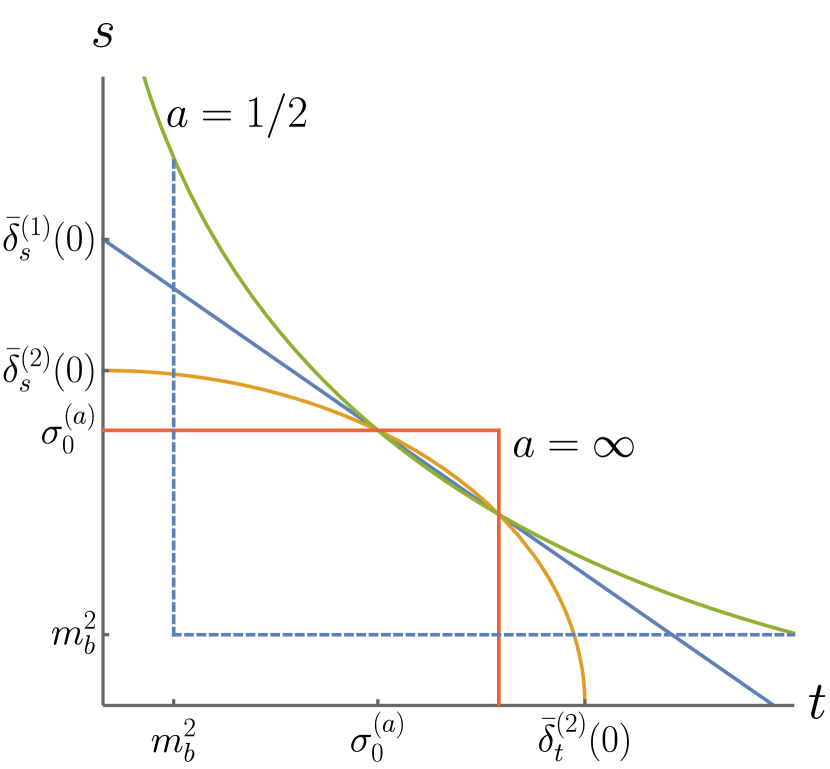
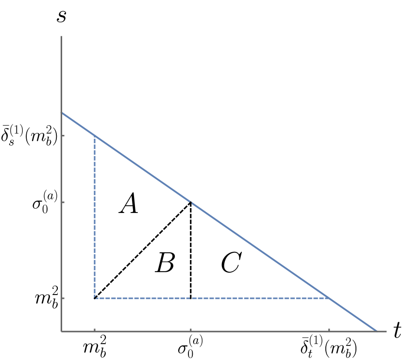
Figure 1: An overview of the duality interval. The left hand figure demonstrates how the parameterisation (25), keeping the quantity ${\sigma}^{(a)}_{0}$ fixed, leads to a range of possible duality windows depending on the value of the parameter $a$. The solid green, blue, yellow, and orange curves correspond to the $a=1/2,1,2,\infty$, cases respectively. In the limit $\tilde{s}_{0}\to\tilde{t}_{0}$ the curves intersect at a single point, ${\sigma}^{(a)}_{0}$. The right hand plot provides a more detailed view of the case $a=1$, which we adopt for our evaluation of the couplings. We note that the choice of duality window has little impact on the final result, cf Tab. 5. The dashed blue line indicates the lower boundary on the duality window, enforced by the restriction that both $t$ and $s$ can only take values above the cut starting at $m_{b}^{2}$. The dashed black line indicates a technical division of the duality region necessary for application of the principal part prescription, cf. (57).

3.4.1 Duality Region as a Function of the Duality Parameter $a$

Finally we turn to the question of the duality region encoded in (21) and derive explicit relations as a function of the parameter $a$. In defining the duality region,

$$\left(\frac{s}{\tilde{s}_{0}}\right)^{a}+\left(\frac{t}{\tilde{t}_{0}}\right)^{a}\leq 1\;,$$ (25)

we follow earlier work Balitsky:1997wi ; Khodjamirian:2020mlb but extend it in that we consider $\tilde{s}_{0},\tilde{t}_{0}$ as a function of the parameter $a$. The solutions to the boundary defined by (25), and which therefore enter (21), are

$$\bar{\delta}^{(a)}_{s}(t)=\tilde{s}_{0}\left(1-\left(\frac{t}{\tilde{t}_{0}}\right)^{a}\right)^{1/a}\,,\quad\bar{\delta}^{(a)}_{t}(s)=\tilde{t}_{0}\left(1-\left(\frac{s}{\tilde{s}_{0}}\right)^{a}\right)^{1/a}\,.$$ (26)

A further quantity that arising from the parameterisation, and thus appearing in results given in the appendix, is

$${\sigma}^{(a)}_{0}=\frac{\tilde{s}_{0}\tilde{t}_{0}}{(\tilde{s}_{0}^{a}+\tilde{t}_{0}^{a})^{1/a}}\;.$$ (27)

Its geometric meaning can be inferred from Fig. 1. It takes on the rôle of the single dispersion effective threshold if $\rho^{\Gamma}\propto\delta(s-t)$ which is the case for a large part of the contributions. Fortunately, variation of the duality parameter $a$ does not lead to large effects when the daughter sum rule is invoked to constrain the SR parameters, as will be discussed in the next section.

We turn to the question of which choice of the parameter $a$ is suitable. We find that in the majority of cases the dependence of the couplings on the duality window is rather limited, as evidenced by Tab. 5. The exceptions are the $B_{1s}$- and the $D^{*}_{s}$-meson cases, showing more significant variation. It has been argued that for the Isgur-Wise function Neubert:1991sp and the small velocity limit Blok:1992fc that $a=1$ is a necessary choice. Whether or not this translates to other cases and in particular to the case at hand is an open question. We adopt $a=1$ as our default choice, and include variations under the duality window in our estimate of the total uncertainty (cf. Sec. 3.5.1).

3.5 Numerical Analysis

Physical input parameters used for the numerical evaluation of the SRs can be found in Tab. 14 in the appendix.

As there are a number of different renormalisation scales involved we discuss them in some detail. The UV scale, $\mu_{\text{UV}}$, has already been mentioned below Eq. (6) and is set to the pole mass $m_{b}(m_{c})^{\textrm{pole}}$. For the LCSR there remains the scale of the coupling $\mu_{\alpha_{s}}$, the mass $\mu_{m}$ (or $\mu_{\textrm{kin}}$ cf. below) and the LC-OPE factorisation scale $\mu_{F}$. We set $\mu_{F}^{2}=m_{B}^{2}-(m_{b}^{kin}(1\,\mbox{GeV}))^{2}(=m_{D}^{2}-m_{c}^{2}(m_{c}))$ which is a standard albeit not a necessary choice and equate $\mu_{\alpha_{s}}=\mu_{F}$. The choice of a mass scale is linked with a choice of mass scheme. For the $B\to\gamma$ form factors we have found Janowski:2021yvz that the $\overline{\text{MS}}$- and the pole-scheme give rise to large effects in either higher twist or at ${\cal O}(\alpha_{s})$ rendering both of them suboptimal. For the $g_{BB^{*}(B_{1})\gamma}$ couplings the evidence for adopting the kinetic- over the $\overline{\text{MS}}$-scheme is less compelling (smaller improvement in twist-convergence). However, in an effort to remain consistent with our previous work Janowski:2021yvz , we choose to adopt the kinetic-scheme for the evaluation of both the FF residues and the effective couplings. As the kinetic mass scheme, originally devised for the inclusive decay operator product expansion (OPE) Bigi:1994em , can be considered as a compromise between the $\overline{\text{MS}}$- and the pole-scheme. Moreover, it is indeed found that the kinetic scheme is stable under scale variation. The kinetic scale is set to $\mu_{\textrm{kin}}\!=\!1\,\mbox{GeV}$, with further details in Janowski:2021yvz . For the $D$-meson decays the situation is different and the $\overline{\text{MS}}$ scheme gives more stable results than the kinetic scheme and we thus employ the $\overline{\text{MS}}$ scheme with the standard choice $\mu_{m}\!=\!m_{c}(m_{c})$. This might not come as a surprise since $m_{c}$ itself is closer to $\mu_{F}$ as compared to the $B$-case.

As indicated in Eqs. (23) and (3.4), to obtain the physical quantities one needs to divide by the decay constant(s) to the same order (cf. Sec. 4 for their discussion). The new inputs are the condensates, given in Tab. 14, and the factorisation scale of the local OPE, denoted by $\mu_{\text{cond}}$, which is set to $\mu_{\text{cond}}=\mu_{F}$ in order to facilitate cancellations in the ratio. A summary of all renormalisation scales is given in Tab. 1 (left). Another aspect is that we drop twist-$4$ corrections, other than the pure quark condensates, as they are incomplete (requiring the inclusion of $4$-particle DAs Janowski:2021yvz ). The resulting uncertainty ought to be captured, at least in part, by the variation of the Borel parameter.

The SR parameters $\{{\sigma}^{(a)}_{0},\hat{M}^{2}\}$ and $\{s^{f_{B}}_{0},M^{2}_{f_{B}}\}$ are determined by a number of constraints. As usual the Borel mass is determined subject to two competing factors, contamination from higher states is effectively suppressed by a small $\hat{M}^{2}$, whilst fast convergence of the LC-OPE favours a large $\hat{M}^{2}$ as higher terms in the expansion are accompanied by ever increasing inverse powers of the Borel mass. The compromise of these two criteria, resulting in an approximately flat curve, is known as the Borel-window. To constrain the effective thresholds $\{\tilde{s}_{0},\tilde{t}_{0}\}$ the, formally exact, daughter SR for the sum of meson masses (28) is employed

$$m_{B}^{2}+m_{B_{1}[B^{*}]}^{2}={2\hat{M}^{4}}\frac{d}{d\hat{M}^{2}}\ln\int_{m_{b}^{2}}^{\bar{\delta}^{(a)}_{s}(m_{b}^{2})}ds\int_{m_{b}^{2}}^{\bar{\delta}^{(a)}_{t}(t)}dt\,e^{-\frac{s+t}{2\hat{M}^{2}}}\,\rho^{\Gamma}_{\parallel[\perp]}(s,t)\;,$$ (28)

with the ratio of $\tilde{s}_{0},\tilde{t}_{0}$ matched to the ratio of meson masses in the respective channels cf. caption of Tab. 2. In addition we impose $\tilde{s}_{0}^{B_{s}}/\tilde{s}_{0}^{B_{d,u}}\approx m_{B_{s}}^{2}/m_{B_{d,u}}^{2}$ and $s_{0}^{f_{B}}/s_{0}^{f_{B^{*}[B_{1}]}}\approx m_{B}^{2}/m_{B^{*}[B_{1}]}^{2}$ to be satisfied reasonably well. We turn to the dependency on a specific duality parameter $a$. It is found that in the $B$-meson cases a single set of SR parameters is sufficient to satisfy (28) to within $\approx 2\%$ for the $a=\{1/2,1,2\}$ cases considered. For the $D$-mesons this no longer holds and a small modification to the SR parameters is made at each value of $a$.

		$\mu_{F}^{2}\!=\!\mu_{\alpha_{s}}^{2}\!=\!\mu_{\text{cond}}^{2}[\,\mbox{GeV}^{2}]$	$\mu_{\text{UV}}[\,\mbox{GeV}]$	$\mu_{m}[\,\mbox{GeV}]$	$\mu_{\textrm{kin}}[\,\mbox{GeV}]$	$\mu_{\alpha_{s}}[\,\mbox{GeV}]$	$\mu_{\text{cond}}[\,\mbox{GeV}]$
$\!\!B$	Kin	$m_{B}^{2}-(m_{b}^{\textrm{pole}})^{2}$	4.78(1.0)	$-$	1.0(4)	4.18(1.5)	3.0(1.0)
$B$	$\overline{\text{MS}}$	$m_{B}^{2}-(m_{b}^{\textrm{pole}})^{2}$	4.78(1.0)	$4.18^{+1.7}_{-1.2}$	$-$	4.18(1.5)	3.0(1.0)
$D$	$\overline{\text{MS}}$	$m_{D}^{2}-m_{c}(m_{c})^{2}$	1.67(30)	$1.27^{+1.5}_{-0.2}$	$-$	$1.27^{+1.0}_{-0.2}$	2.0(1.0)

Table 1: Summary of the scales involved in the determination of the residues (Tab. 6) and coupling constants (Tab. 7) to the left of the double separation line. To the right we have the scale changes used for the best determination of the decay constants (Tab. 8). The quantity $m_{c}(m_{c})$, above, is the $\overline{\text{MS}}$ mass at the scale $m_{c}$. The uncertainty in $\mu_{F}$, for the $B$-meson ($D$-meson), is chosen to be $\Delta\mu_{F}=\pm 1\,\mbox{GeV}$ $(\Delta\mu_{F}=^{+1.0}_{-0.2}\,\mbox{GeV})$.

We consider it worthwhile to comment on the specific numerical values of the thresholds found. The expectation for a single dispersive threshold $s_{0}$ is $(m_{B_{i}}+2m_{\pi})^{2}<s_{0}<(m_{B_{i}}+m_{\rho})^{2}$, and lying closer to the top boundary. Inspecting Tab. 2, we note that this is indeed the case for the single dispersion threshold $s_{0}^{f_{B}}$ but not for the double dispersion threshold ${\sigma}^{(a)}_{0}$ (27). Whereas ${\sigma}^{(a)}_{0}$ takes on a similar rôle to the single dispersive effective threshold, one must remember that it contains additional information on the excited vector meson channel, cf. (26) and might further be a result of the peculiar analytic structure in $(s,t)$ of the LC-OPE.

Let us turn to the correlation imposed on parameters based on physical arguments. Whilst the effective threshold for decay constant $s_{0}^{f_{B}}$ can be independently determined it would contradict the method if it were completely independent of the ${\sigma}^{(a)}_{0}$-threshold, since they are both associated with the same state. A $50\%$-correlation is adopted between the two. The vector versus tensor results are correlated since, by the (exact) equation of motion, their difference is equal to a derivative operator which is numerically (and to some extent parametrically) suppressed at low recoil. In order to remain consistent this implies a correlation of the effective thresholds, as argued in Hambrock:2013zya and more systematically exploited in BSZ15 . The correlations

$$\text{corr}({{\sigma}^{(a)}_{0}}^{V_{\perp}},{{\sigma}^{(a)}_{0}}^{T_{\perp}})|_{B}=\frac{4}{5}\;,\quad\text{corr}({{\sigma}^{(a)}_{0}}^{V_{\parallel}},{{\sigma}^{(a)}_{0}}^{T_{\parallel}})|_{B}=\frac{1}{2}\;,\quad\text{corr}({{\sigma}^{(a)}_{0}}^{V},{{\sigma}^{(a)}_{0}}^{T})|_{D}=\frac{2}{3}\;,$$ (29)

are imposed based on the contribution of the derivative operator to the equations of motion, which is $\approx 10\%$ in the $B\perp$- and $\approx 20\%$ in the $D\perp$-case. In the $B\|$-case the contribution is $\approx 40$-$45\%$.

SR parameters $[\,\mbox{GeV}^{2}]$
	$B_{d}$	$B_{s}$	$B_{u}$		$B_{d,u}$	$B_{s}$
$\{{\sigma}^{(a)}_{0},\hat{M}^{2}\}^{r^{V}_{\perp},r^{T}_{\perp}}$	37.7, 8.00	39.2, 11.0	37.7, 8.00	$\{s_{0},M^{2}\}^{f_{B}}$	34.3, 5.6	35.5, 6.4
$\{{\sigma}^{(a)}_{0},\hat{M}^{2}\}^{r^{V}_{\parallel}}$	43.5, 12.0	45.5, 13.5	43.5, 12.0	$\{s_{0},M^{2}\}^{f_{B^{*}},f_{B^{*}}^{T}}$	34.5, 5.7	35.9, 7.1
$\{{\sigma}^{(a)}_{0},\hat{M}^{2}\}^{r^{T}_{\parallel}}$	42.5, 11.0	44.4, 13.5	42.5, 11.0	$\{s_{0},M^{2}\}^{f_{B_{1}},f_{B_{1}}^{T}}$	38.9, 6.0	40.6, 8.6
	$D_{d}$	$D_{s}$	$D_{u}$		$D_{d,u}$	$D_{s}$
$\{{\sigma}^{(1/2)}_{0},\hat{M}^{2}\}^{r^{V}_{\perp}}$	5.9, 3.1	6.6, 3.4	5.9, 3.1	$\{s_{0},M^{2}\}^{f_{D}}$	5.7, 1.9	6.3, 2.2
$\{{\sigma}^{(1/2)}_{0},\hat{M}^{2}\}^{r^{T}_{\perp}}$	5.9, 2.6	6.6, 2.9	5.9, 2.6	$\{s_{0},M^{2}\}^{f_{D^{*}},f_{D^{*}}^{T}}$	6.1, 1.9	6.9, 2.6
$\{{\sigma}^{(1)}_{0},\hat{M}^{2}\}^{r^{V}_{\perp}}$	6.0, 2.9	6.7, 3.2	6.0, 2.9
$\{{\sigma}^{(1)}_{0},\hat{M}^{2}\}^{r^{T}_{\perp}}$	6.0, 2.4	6.7, 2.7	6.0, 2.4
$\{{\sigma}^{(2)}_{0},\hat{M}^{2}\}^{r^{V}_{\perp}}$	5.7, 2.9	6.5, 3.4	5.7, 2.9
$\{{\sigma}^{(2)}_{0},\hat{M}^{2}\}^{r^{T}_{\perp}}$	5.7, 2.4	6.5, 2.7	5.7, 2.4

Table 2: Summary of the SR parameters used in the determination of the residues for the triangular duality window $a=1$ (cf. Sec. 3.5.1 for comments). The additional threshold parameter is fixed via the ratio of the scalar and vector mesons. For the $B$-mesons $\tilde{t}_{0}/\tilde{s}_{0}=m_{B^{*}}^{2}/m_{B}^{2}\approx 1.02$ and $\tilde{t}_{0}/\tilde{s}_{0}=m_{B_{1}}^{2}/m_{B}^{2}\approx 1.18$ in the $\perp$ and $\|$ directions respectively. In the $D$-meson channels $\tilde{t}_{0}/\tilde{s}_{0}=m_{D^{*}}^{2}/m_{D}^{2}\approx 1.15$. Note the difference between the values of ${\sigma}^{(a)}_{0}$ for the $\perp$- and $\|$-directions reflects the fact that $m^{2}_{B_{1}}/m^{2}_{B^{*}}\approx 1.16$. We remind the reader that in the $B$-meson channels a single set of SR parameters is sufficient to satisfy the daughter SR (28) to within $\approx 2\%$ for all three choices of the duality parameter $a$. For the $B$-meson ($D$-meson) processes we associate a uniform uncertainty to the threshold of $\pm 2.0\,\mbox{GeV}^{2}$ ($\pm 0.5\,\mbox{GeV}^{2}$) and the Borel mass of $\pm 2.0\,\mbox{GeV}^{2}$ ($\pm 0.5\,\mbox{GeV}^{2}$).

twist	pa	DA	$r_{\perp}^{V}(B_{u})$	$r_{\|}^{V}(B_{d})$	$r_{\perp}^{T}(B_{s})$	$r_{\|}^{T}(B_{d})$	$r_{\perp}^{V}(D_{u})$	$r_{\perp}^{V}(D_{d})$	$r_{\perp}^{T}(D_{d})$
1	$-$	PT:$\,{\cal O}{(\alpha_{s}^{0})}$	$-0.116$	$-0.014$	$0.102$	$0.033$	$-0.177$	$0.004$	$0.014$
1	$-$	PT:$\,{\cal O}{(\alpha_{s})}$	$-0.033$	$0.003$	$0.027$	$-0.005$	$-0.047$	$-0.002$	$<10^{-3}$
2	2	$\phi_{\gamma}(u)\,{\cal O}{(\alpha_{s}^{0})}$	$-0.136$	$0.075$	$0.063$	$0.064$	$-0.220$	$0.110$	$0.078$
2	2	$\phi_{\gamma}(u)\,{\cal O}{(\alpha_{s})}$	$-0.028$	$0.015$	$0.015$	$0.015$	$-0.028$	$0.014$	$0.018$
3	2	$\Psi_{(a)}(u)$	$0.011$	$-$	$0.016$	$-0.001$	$0.021$	$-0.010$	$-0.010$
3	2	$\Psi_{(v)}^{(1)}(u)$	$-$	$<10^{-3}$	$0.001$	$<10^{-3}$	$-$	$-$	$0.005$
3	3	$\mathcal{A}(\underline{\alpha})$	$-$	$-$	$<10^{-3}$	$<10^{-3}$	$-$	$-$	$-0.001$
3	3	$\mathcal{V}(\underline{\alpha})$	$-$	$-$	$-0.002$	$-0.003$	$-$	$-$	$-0.014$
4	2	$h_{\gamma}^{(2)}(u)$	$-$	$-0.003$	$<10^{-3}$	$-0.002$	$-$	$-$	$-0.003$
4	2	$\mathbb{A}(u)$	$0.017$	$-0.05$	$-0.003$	$-0.003$	$0.033$	$-0.017$	$-0.006$
4	3	$S(\underline{\alpha})\!+\!\tilde{S}(\underline{\alpha})$	$<10^{-3}$	$<10^{-3}$	$<10^{-3}$	$<10^{-3}$	$-0.003$	$0.001$	$0.002$
4	3	$\sum\limits_{{i=1}}^{4}T_{i}^{(1)}(\underline{\alpha})$	$-0.001$	$<10^{-3}$	$<10^{-3}$	$<10^{-3}$	$-0.007$	$0.003$	$<10^{-3}$
4	3	$S_{\gamma}(\underline{\alpha})$	$-0.008$	$<10^{-3}$	$0.003$	$0.003$	$-0.033$	$-0.033$	$-0.026$
4	3	$T_{4}^{\gamma}(\underline{\alpha})$	$0.002$	$<10^{-3}$	$<10^{-3}$	$<10^{-3}$	$0.007$	$0.007$	$<10^{-3}$
4	$-$	$Q_{q}\left\langle\bar{q}q\right\rangle$	$-$	$0.002$	$-$	$-$	$-$	$-$	$-$
4	$-$	$Q_{b}\left\langle\bar{q}q\right\rangle$	$0.003$	$-0.002$	$0.002$	$0.002$	$-0.021$	$-0.021$	$-0.017$
		Total∗	$-0.290$	$0.070$	$0.223$	$0.102$	$-0.475$	$0.096$	$0.081$

Table 3: A breakdown of contributions according to twist, “pa” = number of partons and the specific DA. The definitions of the DAs can be found in Janowski:2021yvz . The asterisk in total is a reminder that it does not include twist-$4$ contributions not closing under the equations of motion cf. Janowski:2021yvz .

Another relevant aspect concerning the plethora of predictions is that not all channels are of equal quality. This is highlighted by the two separate determinations of the residue, from the vector and tensor interpolating current. Let us define the ratio $U_{B^{(i)}}=g^{T}_{BB^{(i)}\gamma}/g^{V}_{BB^{(i)}\gamma}$ which ideally is close to one. We find reassuringly good values for the $B^{*}$-case $(U_{B^{*0}},U_{B^{*}_{s}},U_{B^{*+}})=(0.99,0.98,0.98)$ , moderate deviations $(U_{D^{*+}},U_{D^{*}_{s}},U_{D^{*0}})=(0.81,0.82,0.91)$ for the $D^{*}$-case and significant deviations $(U_{B_{1}^{0}},U_{B_{1s}},U_{B_{1}^{+}})=(1.35,1.26,1.30)$ for the $B_{1}$-case as anticipated cf. footnote 1. For the $D^{*}$-case it is the accidental cancellation of the two charge contributions in perturbation theory, to be discussed further below, and the sensitivity to higher twist which gives rise to larger deviation from one. For the $B_{1}$-case the concept of a well isolated resonance is not assured and for the $D_{1}$ it simply does not hold cf. also footnote 1. Therefore we do not quote any results for the $D_{1}$ whilst for the $B_{1}$ the results are deemed just marginally acceptable to present.

It is instructive to present a breakdown in terms of charges for comparison with other work and illustrate the, presumably accidental, cancellations in the charged $D$- and $B_{1}$-case which unfortunately implies that these results are less reliable. For definiteness we quote the breakdown for the couplings obtained from the vector interpolating current

$$g_{D_{q}D_{q}^{*}\gamma} \approx -(1.05\,Q_{q}+0.51\,Q_{c})|_{\text{PT}}-1.74\,Q_{q}|_{\text{twist-2}}+\text{ht}\;,$$

$$g_{D_{s}D_{s}^{*}\gamma} \approx -(1.24\,Q_{s}+0.51\,Q_{c})|_{\text{PT}}-1.62\,Q_{s}|_{\text{twist-2}}+\text{ht}\;,$$

$$g_{B_{q}B_{q}^{*}\gamma} \approx -(1.20\,Q_{q}+0.24\,Q_{b})|_{\text{PT}}-1.20\,Q_{q}|_{\text{twist-2}}+\text{ht}\;,$$

$$g_{B_{s}B_{s}^{*}\gamma} \approx -(1.31\,Q_{s}+0.25\,Q_{b})|_{\text{PT}}-1.10\,Q_{s}|_{\text{twist-2}}+\text{ht}\;,$$

$$g_{B_{q}B_{1q}\gamma} \approx +(0.12\,Q_{q}+0.02\,Q_{b})|_{\text{PT}}-1.11\,Q_{q}|_{\text{twist-2}}+\text{ht}\;,$$

$$g_{B_{s}B_{1s}\gamma} \approx -(0.69\,Q_{s}-0.52\,Q_{b})|_{\text{PT}}-1.03\,Q_{s}|_{\text{twist-2}}+\text{ht}\;,$$ (30)

where $Q_{i}$ are the standard quark charges $Q_{b}=Q_{d}=Q_{s}=-\frac{1}{3}$ and $Q_{c}=Q_{u}=\frac{2}{3}$ and “ht” stands for higher twist and $q=u,d$ . The size of the higher twist can be inferred from Tab. 3. The twist-$3$ contribution is up to $5\%$ in some cases and, as previously argued, most twist-$4$ contributions have to be dropped since they are incomplete without the inclusion of $4$-particle DAs (cf. Sec. 3.5.1 for further relevant remarks in this direction).

We now proceed to discuss the numerical features of the $B$- and $D$-meson results in turn. Beginning with the $B$-mesons, for the values given in Tab. 2 we find that the daughter SRs (28) are, in all cases, satisfied to within $\lesssim 2\%$. The continuum contributions range from $\lesssim 25\%$ in the $\perp$-modes to $\lesssim 35\%$ in the $\|$-modes. In the $\perp$-modes the SR is dominated by the perturbative and twist-$2$ contributions which are approximately equal in size and are of the same sign. The remaining contributions make up $\approx 10$-$20\%$ of the total. The story is repeated in the tensor $\|$-modes, however the situation in the vector $\|$-modes is somewhat altered. Here unfortunate cancellations act to suppress the perturbative contribution and the twist-$2$ sector is numerically dominant providing ${\cal O}(80)\%$ of the total value. A breakdown of contributions according to twist is given in Tab. 3 for a representative selection of residues. The ${\cal O}{(\alpha_{s})}$ corrections are mass scheme dependent. In the kinetic mass scheme ($\mu_{\textrm{kin}}=1\,\mbox{GeV}$) employed the NLO results are sizeable, providing a correction of $\approx 20$-$35\%$ and $\approx 20$-$25\%$ at twist-$1$ and -$2$, respectively cf. Tab. 3. The benefit and necessity of an NLO computation is clearly visible in the scale variation plots shown in Fig. 2 as residual effects are then of ${\cal O}(\alpha_{s}^{2})$.

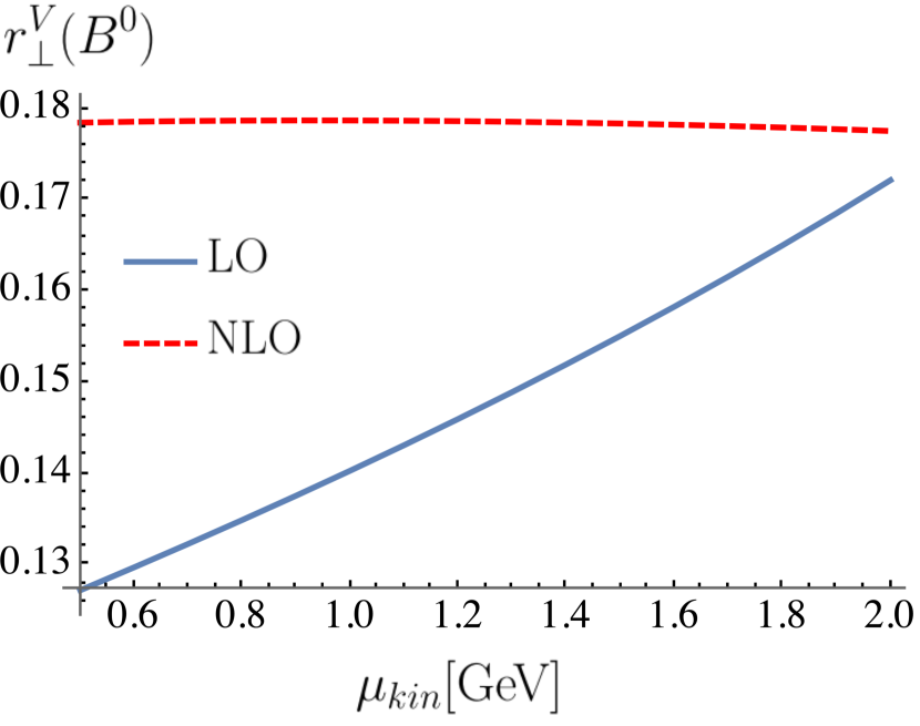
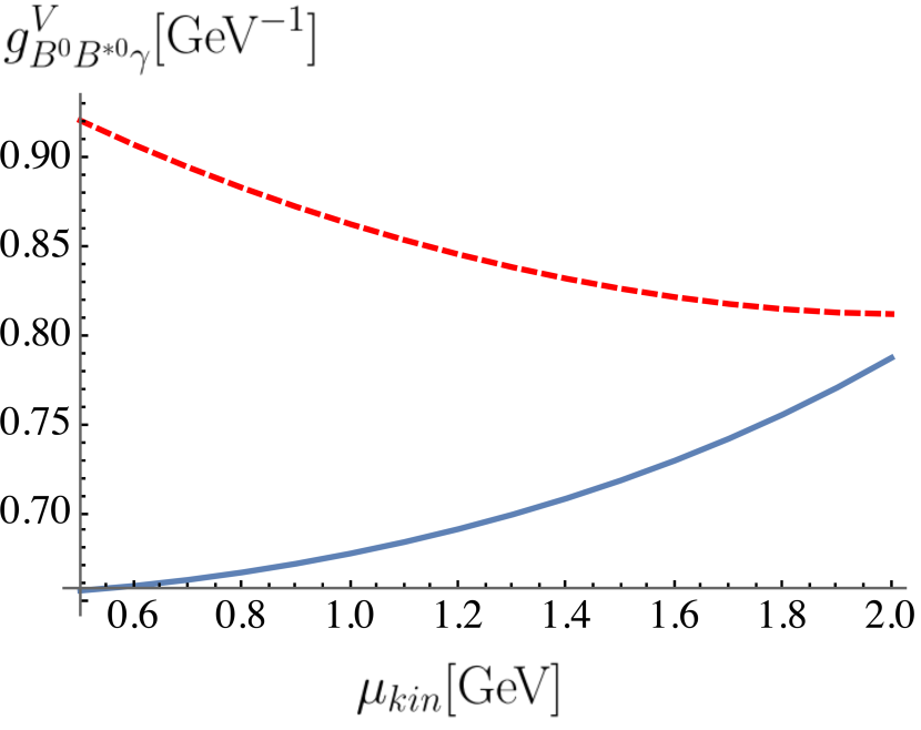
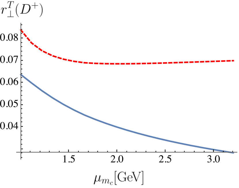
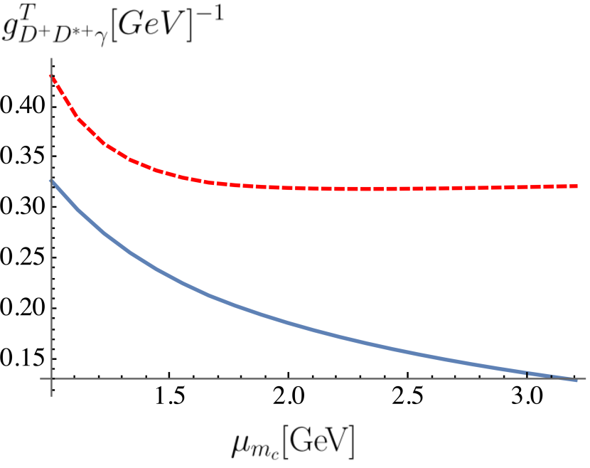
Figure 2: Representative plots highlighting how the NLO result (dashed red) sees a reduction in the mass scheme scale $\mu_{\textrm{kin}}(\mu_{\overline{\text{MS}}})$ as compared to LO (solid blue). We note that in the $B$-meson case the residue generally shows greater stability than the coupling which, in the above cases, inherits the (artificial) scale dependence of $f_{B^{*}}$ which is less pronounced for $f_{D^{*}}$ as the plots show.

The SR parameters for the $D$-mesons are determined subject to the same tests as outlined above. In all cases the continuum contribution remains below $30\%$ and in the neutral modes the daughter SR (28) is satisfied to within $3\%$. In the charged mode the daughter SR shows poor convergence. Again, this is due to the presumably artificial smallness of the perturbative contribution due to cancellation in $Q_{c}$ and $Q_{u}$ (cf. Tab. 3 and (3.5)). In contrast to the $B$-mesons we note that whilst the dominant contribution arises from the twist-$1$ or -$2$ sectors the twist-$3$ and -$4$ sectors are sizeable, in particular in the charged case. The ${\cal O}(\alpha_{s})$ corrections to twist-$2$ range from $\approx 12\%$ of the LO result in the vector modes to $\approx 20\%$ in the tensor modes. In the twist-$1$ sector the tensor modes and the neutral vector mode have radiative corrections ranging between $\approx 2$ - $30\%$. In the charged vector modes, however, the corrections are $>50\%$, due to the previously mentioned large charge cancellation at LO.

	$r_{\perp}^{V}(B_{u})$	$r_{\|}^{V}(B_{d})$	$r_{\perp}^{T}(B_{s})$	$r_{\|}^{T}(B_{d})$	$r_{\perp}^{V}(D_{u})$	$r_{\perp}^{V}(D_{d})$	$r_{\perp}^{T}(D_{d})$
Value	-0.300	0.076	0.224	0.104	-0.473	0.095	0.073
Error	$\phantom{}{}^{+0.034}_{-0.033}$	$\phantom{}{}^{+0.015}_{-0.016}$	$\phantom{}{}^{+0.023}_{-0.024}$	$\phantom{}{}^{+0.015}_{-0.015}$	$\phantom{}{}^{+0.054}_{-0.053}$	$\phantom{}{}^{+0.021}_{-0.021}$	$\phantom{}{}^{+0.020}_{-0.020}$
$\Delta\overline{s_{0}}$	$\pm 0.021$	$\pm 0.007$	$\pm 0.017$	$\pm 0.007$	$\pm 0.033$	$\pm 0.004$	$\pm 0.004$
$\Delta\hat{M}^{2}$	$\phantom{}{}^{+0.005}_{-0.000}$	$\phantom{}{}^{+0.001}_{-0.002}$	$\phantom{}{}^{+0.000}_{-0.002}$	$\phantom{}{}^{+0.000}_{-0.002}$	$\phantom{}{}^{+0.004}_{-0.001}$	$\phantom{}{}^{+0.001}_{-0.002}$	$\phantom{}{}^{+0.004}_{-0.001}$
$\Delta M^{2}_{f_{B}}$	$\phantom{}{}^{+0.000}_{-0.003}$	$\phantom{}{}^{+0.001}_{-0.000}$	$\phantom{}{}^{+0.004}_{-0.000}$	$\phantom{}{}^{+0.001}_{-0.000}$	$\phantom{}{}^{+0.000}_{-0.004}$	$\phantom{}{}^{+0.001}_{-0.000}$	$\phantom{}{}^{+0.001}_{-0.000}$
$\Delta m_{b,c}$	$\pm 0.002$	$\pm 0.004$	$\pm 0.002$	$\pm 0.002$	$\pm 0.003$	$\pm 0.003$	$\pm 0.003$
$\Delta\tau$	$\pm 0.010$	$\pm 0.006$	$\pm 0.005$	$\pm 0.005$	$\pm 0.015$	$\pm 0.008$	$\pm 0.006$
$\Delta\langle\bar{q}q\rangle$	$\pm 0.003$	$\pm 0.001$	$\pm 0.001$	$\pm 0.001$	$\pm 0.005$	$\pm 0.004$	$\pm 0.003$
$\Delta a_{2}$	$\pm 0.020$	$\pm 0.011$	$\pm 0.009$	$\pm 0.010$	$\pm 0.033$	$\pm 0.016$	$\pm 0.012$
$\Delta_{t=3}$	$\pm 0.006$	$<10^{-3}$	$\pm 0.004$	$\pm 0.003$	$\pm 0.011$	$\pm 0.006$	$\pm 0.011$
$\Delta\mu_{\textrm{kin}}$	$\pm 0.003$	$\pm 0.003$	$\pm 0.002$	$\pm 0.004$	$-$	$-$	$-$
$\Delta\mu_{m}$	$-$	$-$	$-$	$-$	$\phantom{}{}^{+0.008}_{-0.001}$	$\phantom{}{}^{+0.004}_{-0.006}$	$\phantom{}{}^{+0.004}_{-0.007}$
$\Delta\mu_{\alpha_{s}}$	$\phantom{}{}^{+0.010}_{-0.003}$	$\phantom{}{}^{+0.001}_{-0.004}$	$\phantom{}{}^{+0.001}_{-0.003}$	$\phantom{}{}^{+0.001}_{-0.001}$	$\phantom{}{}^{+0.002}_{-0.003}$	$<10^{-3}$	$\phantom{}{}^{+0.002}_{-0.001}$
$\Delta\mu_{F}$	$\phantom{}{}^{+0.002}_{-0.000}$	$\phantom{}{}^{+0.001}_{-0.004}$	$\phantom{}{}^{+0.002}_{-0.007}$	$\phantom{}{}^{+0.000}_{-0.001}$	$\phantom{}{}^{+0.005}_{-0.002}$	$\phantom{}{}^{+0.004}_{-0.001}$	$\phantom{}{}^{+0.000}_{-0.001}$
$\Delta\mu_{\text{UV}}$	$-$	$-$	$\pm 0.002$	$\pm 0.001$	$-$	$-$	$\pm 0.001$
$\Delta\frac{{\left\langle\bar{q}q\right\rangle}}{{\left\langle\bar{s}s\right\rangle}}$	$-$	$-$	$\pm 0.002$	$-$	$-$	$-$	$-$
$\Delta\Sigma$	$\pm 0.001$	$\pm 0.003$	$\pm 0.006$	$\pm 0.006$	$\pm 0.013$	$\pm 0.002$	$\pm 0.006$

Table 4: Breakdown of the main contributions to the uncertainty for a representative selection of residues. $\Delta\overline{s_{0}}$ includes the combined uncertainty, incorporating correlations, due varying all effective thresholds, cf. discussion above (9). $\Delta_{t=3}$ contains the total uncertainty due to all twist-$3$ hadronic parameters $\{f_{3\gamma},\omega_{\gamma}^{A},\omega_{\gamma}^{V}\}$. The uncertainty due to the choice of duality region is encapsulated in the quantity $\Delta\Sigma$ which represents the standard deviation of the $a=\{1/2,1,2\}$ evaluations. The total uncertainty, which also includes smaller contributions such as the gluon condensate, is obtained by added uncertainties in quadrature.

The uncertainty due to the input parameters is estimated by varying each parameter, within the given interval, in turn and adding each individual uncertainty in quadrature. To incorporate correlations between the various thresholds, discussed previously, we generate 300 samples of the thresholds according to a Gaussian distribution such that the mean corresponds to the central value of each threshold and the standard deviation reproduces the associated uncertainty. We then evaluate the desired quantity for each of these samples, taking the standard deviation of the resulting points to be the uncertainty due to threshold variation. Our predictions for the couplings are given as the mean value of the vector and tensor interpolating current determinations. We estimate the associated uncertainty as the standard deviation of the two evaluations. Moreover, the uncertainty associated with varying the duality window is taken to be the standard deviation of the $a=\{1/2,1,2\}$ determinations (cf. Tab. 5). This provides a small contribution in the $B$-meson cases, but notably a more significant contribution in the $D_{s}$ mode. Adding in quadrature the uncertainty from all sources, we obtain the total uncertainty as quoted in Tab. 7.

	$g_{B_{d}B_{d}^{*}\gamma}$	$g_{B_{s}B_{s}^{*}\gamma}$	$g_{B_{u}B_{u}^{*}\gamma}$	$g_{B_{d}B_{1d}\gamma}$	$g_{B_{s}B_{1s}\gamma}$	$g_{B_{u}B_{1u}\gamma}$	$g_{D_{d}D_{d}^{*}\gamma}$	$g_{D_{s}D_{s}^{*}\gamma}$	$g_{D_{u}D_{u}^{*}\gamma}$
$a=1/2$	$0.86$	$0.96$	$-1.43$	$0.35$	$0.42$	$-0.70$	$0.38$	$0.69$	$-2.03$
$a=1$	$0.86$	$0.95$	$-1.44$	$0.37$	$0.44$	$-0.72$	$0.40$	$0.60$	$-2.11$
$a=2$	$0.86$	$0.94$	$-1.43$	$0.40$	$0.48$	$-0.74$	$0.40$	$0.52$	$-2.03$

Table 5: Values of the coupling for different values of the duality parameter $a$ (cf. Sec. 3.4.1 and (25)). The majority of couplings show little dependence on the duality parameter $a$. Notable exceptions are the neutral $B_{1}$-couplings and the charged $D^{*}$-couplings. This does not come as a surprise as precisely those are plagued by, unfortunate, cancellations in the perturbative contribution of the $Q_{b,c}$- and $Q_{q}$-parts (cf. end of Sec. 3.5.1 for comments).

The final values for the residues and the couplings are shown in Tabs. 6 and 7 respectively. The value of the coupling presented in the table is the average of the vector and tensor determinations.

		$r_{\perp}^{V}$	$r_{\perp}^{T}$	$r_{\parallel}^{V}$	$r_{\parallel}^{T}$
$\mu_{\textrm{kin}}=1.0\,\mbox{GeV}$	$B_{d}$	$\phantom{-}0.179^{+0.019}_{-0.019}$	$0.171^{+0.018}_{-0.020}$	$0.076^{+0.015}_{-0.016}$	$0.104^{+0.015}_{-0.015}$
	$B_{s}$	$\phantom{-}0.235^{+0.024}_{-0.025}$	$0.224^{+0.023}_{-0.024}$	$0.114^{+0.016}_{-0.018}$	$0.146^{+0.017}_{-0.017}$
	$B_{u}$	$-0.300^{+0.034}_{-0.033}$	$-0.284^{+0.033}_{-0.031}$	$-0.159^{+0.031}_{-0.029}$	$-0.199^{+0.028}_{-0.028}$
$\mu_{\overline{\text{MS}}}=m_{c}(m_{c})$	$D_{d}$	$0.095^{+0.021}_{-0.021}$	$0.073^{+0.020}_{-0.020}$	$-$	$-$
	$D_{s}$	$0.172^{+0.033}_{-0.029}$	$0.140^{+0.048}_{-0.046}$	$-$	$-$
	$D_{u}$	$-0.473^{+0.054}_{-0.053}$	$-0.412^{+0.049}_{-0.049}$	$-$	$-$

Table 6: The residues (2), related to form factors, for the $B$- and $D$-mesons. The former are determined in the kinetic scheme and the latter in the $\overline{\text{MS}}$ scheme.

3.5.1 Comparison with Literature and Experiment

It is of interest to compare to the existing literature and experiment. The values of the couplings obtained in this work, which constitute the mean value of the tensor and vector determinations, along with determinations from other computations as well as experiment are collected in Tab. 7. Unfortunately only two of the six couplings can be inferred from experiment as the widths of the vector mesons are too often unknown. Moreover, in this section we use $(B_{u},B_{d},D_{d},D_{u})\to(B^{+},B^{0},D^{+},D^{0})$ which is the notation often used in experiment.

units [$\,\mbox{GeV}^{-1}$]	$g_{B^{0}B^{*0}\gamma}$	$g_{B_{s}B_{s}^{*}\gamma}$	$g_{B^{+}B^{*+}\gamma}$	$g_{D^{+}D^{*+}\gamma}$	$g_{D_{s}D_{s}^{*}\gamma}$	$g_{D^{0}D^{*0}\gamma}$
This work	$\textrm{\phantom{-}}0.86^{+0.15}_{-0.15}$	$0.95^{+0.15}_{-0.16}$	-$1.44^{+0.27}_{-0.26}$	$0.40^{+0.12}_{-0.13}$	$0.60^{+0.19}_{-0.18}$	-$2.11^{+0.35}_{-0.34}$
LCSR (NLL) Li:2020rcg	-$0.91^{+0.12}_{-0.13}$	-$0.74^{+0.09}_{-0.10}$	$1.44^{+0.22}_{-0.20}$	-$0.15^{+0.11}_{-0.10}$	-$0.079^{+0.086}_{-0.078}$	$1.48^{+0.29}_{-0.27}$
HH$\chi$PT Amundson:1992yp	-$1.01^{+0.05}_{-0.05}$	-$0.70^{+0.06}_{-0.06}$	$1.45^{+0.11}_{-0.11}$	-$0.27^{+0.05}_{-0.05}$	$0.041^{+0.056}_{-0.056}$	$2.19^{+0.11}_{-0.11}$
VMD $\!+\!$ HQET Colangelo:1993zq	-$0.58^{+0.12}_{-0.10}$	$-$	$0.99^{+0.19}_{-0.13}$	-$0.29^{+0.19}_{-0.11}$	-$0.19^{+0.19}_{-0.08}$	$1.60^{+0.35}_{-0.45}$
CQM $\!+\!$ HQET Cheung:2014cka	-$0.82^{+0.06}_{-0.05}$	$-$	$1.45^{+0.11}_{-0.12}$	-$0.38^{+0.05}_{-0.04}$	$-$	$1.91^{+0.09}_{-0.09}$
RQM Goity:2000dk	-$0.93^{+0.05}_{-0.05}$	$0.65^{+0.03}_{-0.03}$	$1.66^{+0.11}_{-0.11}$	-$0.44^{+0.06}_{-0.06}$	-$0.19^{+0.03}_{-0.03}$	$2.15^{+0.11}_{-0.11}$
Lattice Becirevic:2009xp ∗, Donald:2013sra ‡	$-$	$-$	$-$	-$0.20^{+0.30}_{-0.30}\phantom{}{}^{*}$	$0.11^{+0.02}_{-0.02}\phantom{}{}^{\ddagger}$	$2.00^{+0.60}_{-0.60}\phantom{}{}^{*}$
Experiment PDG	$-$	$-$	$-$	$0.47^{+0.07}_{-0.07}$	$-$	$1.77^{+0.16}_{-0.16}\phantom{}{}^{\dagger}$
units [$\,\mbox{GeV}^{-1}$]	$g_{B^{0}B^{0}_{1}\gamma}$	$g_{B_{s}B_{1s}\gamma}$	$g_{B^{+}B^{+}_{1}\gamma}$
This work	$0.37^{+0.12}_{-0.12}$	$0.44^{+0.12}_{-0.12}$	-$0.72^{+0.21}_{-0.20}$

Table 7: ^†The experimental value of $g_{D^{0}D^{*0}\gamma}$ requires the use of isospin symmetry to deduce the width of the $D^{*0}$ cf. the main text in Sec. 3.5.1. Here we take $(B_{u},B_{d},D_{d},D_{u})\to(B^{+},B^{0},D^{+},D^{0})$ to conform to PDG. Note that the sign cannot be determined from experiment and that for the theory results it is convention dependent cf. (37). We further note that $g_{B_{s}B_{s}^{*}\gamma}=\frac{f_{B_{s}}}{f_{B_{s}^{*}}}\frac{m_{B_{s}^{*}}}{m_{B_{s}}}|\mu|\approx 1.18\,\mbox{GeV}^{-1}$ with $|\mu|=1.13\,\mbox{GeV}^{-1}$ from Aditya:2012im , deduced from $D^{*}$-decays and subject to $1/m_{c}$ corrections, is rather close to our value given the difference in methods. Whereas Ref. Aliev:1995zlh established that the $D$-couplings can be determined from LCSR we do not include the LO results presented therein as the input is outdated and a numerical comparison seems of limited use.

With regards to the two experimental values, we update the analysis in Becirevic:2009xp and make some further comments. We first turn to the $D^{*+}$, for which the width $\Gamma(D^{*+})=83.4(18)\,\mbox{keV}$ and branching fraction $B(D^{*+}\to D^{+}\gamma)=0.016(4)$ are known PDG , and with (2) give $|g_{D^{+}D^{*+}\gamma}|=0.47(7)\,\mbox{GeV}^{-1}$ instead of the previous $0.50(8)\,\mbox{GeV}^{-1}$ in Becirevic:2009xp . For $D^{*0}$ the width is unknown and one needs to rely on isospin to infer it Becirevic:2009xp . First we deduce $g_{c}$, related to the $D^{*+}D\pi$-coupling, as $g_{c}=0.57(7)$, which is down from $0.61(7)$ in Becirevic:2009xp . Considering all decay channels one then obtains $\Gamma(D^{*0})=56.5(14.0)\,\mbox{keV}$, down from $68(17)\,\mbox{keV}$ in Becirevic:2009xp . Using the branching fraction $B(D^{*0}\to D^{0}\gamma)=0.353(9)\,\mbox{keV}$, down from $0.381(29)\,\mbox{keV}$ we get $|g_{D^{0}D^{*0}\gamma}|=1.77(16)\,\mbox{GeV}^{-1}$, down from $2.02(26)\,\mbox{GeV}^{-1}$ in Becirevic:2009xp .

Our result $g_{D^{0}D^{*0}\gamma}=2.11^{+0.35}_{-0.34}\,\mbox{GeV}^{-1}$ is compatible with experiment and so are the results of the other method. Our value for $g_{D^{+}D^{*+}\gamma}=0.40^{+0.12}_{-0.13}\,\mbox{GeV}^{-1}$ is again compatible with the new experimental value $|g_{D^{+}D^{*+}\gamma}|=0.47(7)\,\mbox{GeV}^{-1}$. Differences between this work and the LCSR computation Li:2020rcg are noticeable and can be at least partially accounted for by computational differences. Firstly, we have computed twist-$1$ ${\cal O}(\alpha_{s})$-corrections whereas they did not. Secondly, we include linear quark mass correction at LO and in the magnetic vacuum susceptibility $\chi_{q}$ (cf. section 3.2.1 in Janowski:2021yvz ). Third and most importantly, we drop twist-$4$ corrections other than the $Q_{b}{\left\langle\bar{q}q\right\rangle}$ condensate cf. previous section. For the $B$-meson case the twist-$4$ corrections are not large and the impact is small and the differences can be attributed to the first two cases. For the $D$-mesons higher twist corrections are more important per se, as they are less convergent. In addition, for the charged case perturbation theory is presumably artificially suppressed which makes these results less reliable in general. Another important aspect is that in the charged case the inclusion of $S_{\gamma}$ and $T_{4\gamma}$ is definitely incomplete as the photon can connect to the external states. A sign of this is that in the neutral case the twist-$4$ contributions cancel, whereas in the charged case they are additive cf. Tab. 3.

The lattice determination $g_{D_{s}D^{*}_{s}\gamma}|_{\mbox{\cite[cite]{\@@bibref{Authors Phrase1YearPhrase2}{Donald:2013sra}{\@@citephrase{(}}{\@@citephrase{)}}}}}=0.11(2)$ is approximately three standard deviations lower than our value $g_{D_{s}D^{*}_{s}\gamma}=0.60(19)$. This is where the breakdown (3.5) is useful. We find $g_{D_{s}D^{*}_{s}\gamma}\approx-0.6\,Q_{c}-3.0\,Q_{s}$ and from Fig. 3 in Donald:2013sra one deduces $g_{D_{s}D^{*}_{s}\gamma}|_{\mbox{\cite[cite]{\@@bibref{Authors Phrase1YearPhrase2}{Donald:2013sra}{\@@citephrase{(}}{\@@citephrase{)}}}}}\approx-0.66Q_{c}-1.65Q_{s}$. Whilst it is noted that in both cases the charm and strange quark contribution largely cancel each other, the effect is more pronounced for the lattice result. The charm contribution is rather close and the deviation is in the strange quark part with almost a factor 2 difference, which seems large but not as large as the initial number would suggest. It is instructive to investigate the $D^{*+}\to D^{+}\gamma$ case as by $D$-spin symmetry, one would roughly expect a $20$-$30\%$-deviation. For our computation this is indeed the case $g_{D^{+}D^{*+}\gamma}\approx-0.65\,Q_{c}-2.5\,Q_{d}\approx 0.40(13)$, which does agree reasonably well with experiment $g_{D^{+}D^{*+}\gamma}=0.47(7)$ (cf. Tab. 7). Concerning the question of $D$-spin breaking, some further guidance can be obtained from the lattice evaluation of the $D_{d,s}\to\gamma$ form factors Desiderio:2020oej . The fits to a linear and an extended pole model are in agreement with $20$-$30\%$ $D$-spin breaking close to the kinematic endpoint. If the same level of $D$-spin breaking were valid at the $m_{D^{*}}^{2}$-pole, which some past experience suggests, then $g_{D^{+}D^{+*}\gamma}$ and $g_{D_{s}D^{*}_{s}\gamma}$ should not deviate considerably more than $20$-$30\%$ from each other. If the former is true then this gives rise to a tension between the experimental $g_{D^{+}D^{*+}\gamma}=0.47(7)$ and the lattice determination of $g_{D_{s}D^{*}_{s}\gamma}|_{\mbox{\cite[cite]{\@@bibref{Authors Phrase1YearPhrase2}{Donald:2013sra}{\@@citephrase{(}}{\@@citephrase{)}}}}}=0.11(2)$. In conclusion it remains somewhat unclear what the resolution of this puzzle is. Whereas the sum rule results seems consistent, we wish to emphasise that, in exactly these modes, the sum rules are not the best of their kind for various reasons. It may well be that the level of cancellations between the strange and the charm charge contributions are so severe that past experience is overthrown. It would be helpful to have further lattice determinations of these couplings and in particular a more precise one for $g_{D^{+}D^{+*}\gamma}$.

4 The $f_{H},f_{H^{*}},f_{H_{1}},f_{H^{*}}^{T}$ and $f_{H_{1}}^{T}$ Decay Constants from QCD Sum Rules

The main reason for computing the decay constants is that to the best of our knowledge $\{f_{H^{*}}^{T},f_{H_{1}}^{T}\}$, required for the relation between the couplings and the (form factor) residues (2), have not been subjected to a QCD SR evaluation and are thus new. The quantities $f_{B}$ and $f_{B^{*}}$ have previously been computed Jamin:2001fw ; Gelhausen:2013wia ; Wang:2015mxa to NLO with even partial NNLO results. We recompute these SRs and find agreement with the analytic expressions of the first two references. In the work Wang:2015mxa the ${\cal O}(\alpha_{s})\langle\bar{q}q\rangle$ corrections were computed independently and we do disagree with some the expression e.g. the incomplete Gamma function. Compare equation (21) Wang:2015mxa versus (B) and equation (59) in Gelhausen:2013wia .

4.1 The Computation

The starting points for the computations are the “diagonal” correlation functions

$$\Gamma^{f_{B}}(p)\; = \;i\int_{x}e^{ip\!\cdot\!x}\langle 0|T\{J_{B}(x)J_{B}^{\dagger}(0)\}|0\rangle\; = \;\Gamma_{f_{B}}(p^{2})\;,$$

$$\Gamma^{f_{B^{*}}}_{\alpha\beta}(p)\; = \;i\int_{x}e^{ip\!\cdot\!x}\langle 0|T\{J_{\alpha}(x)J^{\dagger}_{\beta}(0)\}|0\rangle\; = \;V_{\alpha\beta}\Gamma_{f_{B^{*}}}(p^{2})+\tilde{V}_{\alpha\beta}\tilde{\Gamma}_{f_{B^{*}}}(p^{2})\;,$$

$$\Gamma^{f_{B^{*}}^{T}}_{\alpha\beta\gamma\delta}(p)\; = \;i\int_{x}e^{ip\!\cdot\!x}\langle 0|T\{J^{T}_{\alpha\beta}(x)J^{T\dagger}_{\gamma\delta}(0)\}|0\rangle\; = \;T_{[\alpha\beta][\gamma\delta]}\Gamma_{f_{B^{*}}^{T}}(p^{2})+\tilde{T}_{\alpha\beta\gamma\delta}\tilde{\Gamma}_{f_{B^{*}}^{T}}(p^{2})\;,$$

where we have taken $H=B$ for concreteness again. Above $J_{\alpha}=\bar{q}\gamma_{\alpha}b$, $J^{T}_{\alpha\beta}=\bar{q}\sigma_{\alpha\beta}b$ and the previously encountered $J_{B}$ is given in (10). The Lorentz structures are

$$V_{\alpha\beta}=\frac{p_{\alpha}p_{\beta}}{p^{2}}-g_{\alpha\beta}\;,\quad\tilde{V}_{\alpha\beta}=p_{\alpha}p_{\beta}\;,\quad T_{\alpha\beta\gamma\delta}=-g_{\alpha\gamma}\frac{p_{\gamma}p_{\delta}}{p^{2}}\;,\quad\tilde{T}_{\alpha\beta\gamma\delta}=\tensor{\varepsilon}{{}_{\alpha}{}_{\beta}^{\bar{\alpha}}{}^{\bar{\beta}}}\,\tensor{\varepsilon}{{}_{\gamma}{}_{\delta}^{\bar{\gamma}}{}^{\bar{\delta}}}T_{\bar{\alpha}\bar{\beta}\bar{\gamma}\bar{\delta}}\;.$$

The Lorentz invariant functions are related to the hadronic quantities as follows

$$\Gamma_{f_{B}}=\frac{m_{B}^{4}f_{B}^{2}}{m_{B}^{2}-p^{2}}+\dots\;,\qquad\Gamma_{f_{B^{*}}}=\frac{m_{B^{*}}^{2}f_{B^{*}}^{2}}{m_{B^{*}}^{2}-p^{2}}+\dots\;,\qquad\Gamma_{f_{B^{*}}^{T}}=\frac{m_{B^{*}}^{2}(f_{B^{*}}^{T})^{2}}{m_{B^{*}}^{2}-p^{2}}+\dots\;,$$ (31)

and the remaining structure $\tilde{\Gamma}_{f_{B^{*}}}(p^{2})$ is related to $\Gamma_{f_{B}}(p^{2})$ up to contact terms by the equation of motion. The correlation functions for the $\{f_{B_{1}},f_{B_{1}}^{T}\}$ decay constants follow with rules for the insertion of the $\gamma_{5}$ into the currents cf. (B) and $B^{*}\to B_{1}$ in (31) following the ideas in Gratrex:2018gmm .

The generic SR is parametrised by

$$f_{B_{(i)}}^{2}=\frac{e^{\frac{m_{B_{(i)}}^{2}}{M_{f_{B_{(i)}}}^{2}}}}{\omega_{B_{(i)}}}\Big{(} \int_{m_{b}^{2}}^{s^{f_{B_{(i)}}}_{0}}ds\,e^{-\frac{s}{M_{f_{B_{(i)}}}^{2}}}\,\rho_{f_{B_{(i)}}}(s)+$$ (32)

$$e^{\frac{-m_{b}^{2}}{M_{f_{B_{(i)}}}^{2}}}\left[c_{{\left\langle\bar{q}q\right\rangle}}^{f_{B_{(i)}}}m_{b}{\left\langle\bar{q}q\right\rangle}+c_{{\left\langle G^{2}\right\rangle}}^{f_{B_{(i)}}}{\left\langle G^{2}\right\rangle}+\frac{m_{b}}{M_{f_{B_{(i)}}}^{2}}c_{{\left\langle\bar{q}Gq\right\rangle}}^{f_{B_{(i)}}}{\left\langle\bar{q}Gq\right\rangle}\right]\Big{)}\;,$$

where $f_{B_{(i)}}$ stands for any $\{f_{B},f_{B^{*}},f_{B^{*}}^{T},f_{B_{1}},f_{B_{1}}^{T}\}$, $\omega_{B}=m_{B}^{4}/(m_{b}+m_{q})^{2}$ and $\omega_{B_{(i)}}=m_{B_{(i)}}^{2}$ otherwise. The local OPE is performed up to $\dim\leq 5$ including ${\cal O}{(\alpha_{s})}$ corrections to both the perturbative and quark condensate contributions. Four quark condensates ($d=6$) give contributions at the sub per mille level and are omitted. We have checked that all the scale dependences, due to NLO computations, are correct. This includes the cancellation of the condensate scale, denoted by $\mu_{\text{cond}}$, up to ${\cal O}(\alpha_{s}^{2})$ as well as the anomalous scaling of the scalar and transverse decay constants (7). Explicit results are given in App. B.

$f_{B_{(i)}}\backslash B_{(i)}(\,\mbox{MeV})$	$B(5280)$	$B_{s}(5367)$	$B^{*}(5325)$	$B^{*}_{s}(5415)$	$B_{1}(5726)$	$B_{1s}(5829)$
lattice Aoki:2019cca ; Lubicz:2017asp	190.0(1.3)	230.3(1.3)	186.4(7.1)	223.1(5.6)	$-$	$-$
experiment PDG	188(17)(18)	$-$	$-$	$-$	$-$	$-$
SR Gelhausen:2013wia	$207^{+17}_{-9}$	$242^{+17}_{-12}$	$210^{+10}_{-12}$	$251^{+14}_{-16}$	$335^{+18}_{-18}$ Wang:2015mxa	$348^{+18}_{-18}$ Wang:2015mxa
SR Lucha:2010ea	$193.4(16.6)$	$232.5(21.0)$	$-$	$-$	$-$	$-$
this work	$192^{+20}_{-19}$	$225^{+21}_{-20}$	$209^{+23}_{-22}$	$245^{+24}_{-23}$	$247^{+31}_{-29}$	$305^{+27}_{-26}$
$\delta_{\text{PT}},\;\delta_{\left\langle\bar{q}q\right\rangle}$	0.18, -0.03	0.20, -0.02	0.10, -0.08	0.13, -0.07	0.11, -0.09	0.14, -0.05
$s^{f_{B_{(i)}}}_{0}$, $M^{2}_{f_{B_{(i)}}}$	34.4, 5.7	35.6, 6.6	34.9, 6.2	36.2, 6.9	38.1, 5.7	40.9, 8.1
$f^{T}_{B_{(i)}}\backslash B_{(i)}(\,\mbox{MeV})$			$B^{*}(5325)^{T}$	$B^{*}_{s}(5415)^{T}$	$B_{1}(5726)^{T}$	$B_{1s}(5829)^{T}$
this work			$200^{+21}_{-20}$	$236^{+22}_{-21}$	$230^{+29}_{-28}$	$285^{+25}_{-24}$
$\delta_{\text{PT}},\;\delta_{\left\langle\bar{q}q\right\rangle}$			0.11, -0.08	0.14, -0.06	0.11, -0.09	0.14, -0.05
$s_{0}^{f_{B_{(i)}}}$, $M^{2}_{f_{B_{(i)}}}$			34.9, 6.2	36.3, 7.4	38.1, 5.7	40.9, 8.6
$f^{(T)}_{D_{(i)}}\backslash D_{(i)}(\,\mbox{MeV})$	$D(1865)$	$D_{s}(1968)$	$D^{*}(2007)$	$D^{*}_{s}(2112)$	$D^{*}(2007)^{T}$	$D^{*}_{s}(2112)^{T}$
lattice Aoki:2019cca ; Lubicz:2017asp	209.0(2.4)	248.0(1.6)	223.5(8.7)	268.8(6.5)	$-$	$-$
experiment PDG	203.7(47)(6)	257.8(41)(1)	$-$	$-$	$-$	$-$
SR Gelhausen:2013wia	$201^{+12}_{-13}$	$238^{+13}_{-23}$	$242^{+20}_{-12}$	$293^{+19}_{-14}$	$-$	$-$
SR Lucha:2010ea	$206.2(12.4)$	$245.3(20.2)$	$-$	$-$	$-$	$-$
this work	$190^{+15}_{-15}$	$226^{+17}_{-17}$	$227^{+18}_{-17}$	$279^{+19}_{-19}$	$202^{+16}_{-16}$	$256^{+16}_{-17}$
$\delta_{\text{PT}},\;\delta_{\left\langle\bar{q}q\right\rangle}$	0.24, 0.02	0.28, 0.03	0.05, -0.15	0.11, -0.11	0.07, -0.14	0.14, -0.10
$s_{0}^{f_{B_{(i)}}}$, $M^{2}_{f_{B_{(i)}}}$	5.7, 1.9	6.3, 2.2	5.9, 2.0	6.8, 2.7	5.8, 2.2	6.9, 3.0

Table 8: QCD SR results for the decay constants, in units of  MeV, with the exception of the Borel parameter and the threshold which are given in $\,\mbox{GeV}^{2}$-units. The kinetic ($\mu_{\textrm{kin}}\!=\!1\,\mbox{GeV}$) and $\overline{\text{MS}}$ ($\mu_{m}\!=\!m_{c}(m_{c})$) schemes are employed for the $B$- and $D$-meson case respectively. Input values are given in Tab. 14. For the $B(D)$-meson SR a uniform uncertainty $\Delta s_{0}\!=\!\pm 1.5\,\mbox{GeV}^{2}$ ($\Delta s_{0}\!=\!\pm 0.5\,\mbox{GeV}^{2}$), $\Delta M^{2}\!=\!\pm 1.5\,\mbox{GeV}^{2}$ ($\Delta M^{2}\!=\!\pm 0.5\,\mbox{GeV}^{2}$) is applied to the threshold and the Borel parameter. The slightly smaller uncertainty assigned to the decay constant SR parameters versus those of the residues reflects the fact that the daughter SR is satisfied to within $\approx 0.5\%$ in the former but only to within $\approx 2\%$ in the latter. The relative size of the radiative corrections are denoted by $\delta X$ such that $f_{B_{(i)}}|_{X_{\text{NLO}}}\!=\!f_{B_{(i)}}|_{X_{\text{LO}}}(1\!+\!\delta_{X})$, with $X=\{\text{PT},{\left\langle\bar{q}q\right\rangle}\}$. For comparison we include the most recent lattice determinations. The $J^{P}\!=\!0^{-}$ decay constants are taken from Aoki:2019cca which averages over values in Bazavov:2017lyh ; Gambino:2017vkx ; Hughes:2017spc ; McNeile:2011ng and Yang:2014sea ; Bazavov:2011aa ; Boyle:2017jwu ; Davies:2010ip ; Na:2012iu for the $B$- and $D$-mesons, respectively. For the $J^{P}\!=\!1^{-}$ states we quote the values obtained in Lubicz:2017asp . The experimental values are from the PDG review and the extraction of the decay constants involve the CKM matrix $|V_{\textrm{ub}}|$ and $|V_{\textrm{cd(s)}}|$ as inputs. The PDG-error is from the experiment and the CKM input in the first and second parentheses respectively. Note that the central values for $f_{B_{1}}$ and $f_{B_{1s}}$ from Wang:2015mxa deviate considerably from ours which might be due to discrepancies in the ${\cal O}(\alpha_{s})\langle\bar{q}q\rangle$-corrections (cf. remarks at the end of the first paragraph in Sec. 4).

The PDG value, for which the CKM matrix elements $|V_{\textrm{cd(s)}}|$ are inputs, deviates close to three standard deviations from the lattice result.

	$f_{B}$	$f_{B_{s}}$	$f_{B^{*}}$	$f_{B^{*}}^{T}$	$f_{D}$	$f_{D_{s}}$	$f_{D^{*}}$	$f_{D^{*}}^{T}$
Value	192.3	224.8	209.0	199.7	189.6	225.7	226.7	202.1
Error	$\phantom{}{}^{+19.7}_{-18.6}$	$\phantom{}{}^{+21.3}_{-20.3}$	$\phantom{}{}^{+22.6}_{-21.2}$	$\phantom{}{}^{+20.7}_{-19.5}$	$\phantom{}{}^{+14.7}_{-15.4}$	$\phantom{}{}^{+17.1}_{-17.4}$	$\phantom{}{}^{+18.3}_{-16.5}$	$\phantom{}{}^{+16.0}_{-16.3}$
$\Delta s_{0}^{f_{B}}$	$\phantom{}{}^{+11.0}_{-9.5}$	$\phantom{}{}^{+12.3}_{-10.8}$	$\phantom{}{}^{+12.0}_{-10.4}$	$\phantom{}{}^{+10.7}_{-9.2}$	$\phantom{}{}^{+10.5}_{-8.9}$	$\phantom{}{}^{+10.8}_{-9.2}$	$\phantom{}{}^{+13.1}_{-11.1}$	$\phantom{}{}^{+11.6}_{-9.9}$
$\Delta M^{2}_{f_{B}}$	$\phantom{}{}^{+0.0}_{-1.8}$	$\phantom{}{}^{+0.0}_{-2.0}$	$\phantom{}{}^{+0.0}_{-1.0}$	$\phantom{}{}^{+0.0}_{-0.5}$	$\phantom{}{}^{+0.0}_{-1.7}$	$\phantom{}{}^{+0.0}_{-1.6}$	$\phantom{}{}^{+0.6}_{-0.2}$	$\phantom{}{}^{+0.8}_{-0.0}$
$\Delta m_{h}$	$\phantom{}{}^{+11.4}_{-11.7}$	$\phantom{}{}^{+11.8}_{-12.0}$	$\phantom{}{}^{+14.1}_{-14.6}$	$\phantom{}{}^{+12.9}_{-13.4}$	$\phantom{}{}^{+2.0}_{-1.9}$	$\phantom{}{}^{+2.0}_{-1.8}$	$\pm 6.1$	$\pm 4.4$
$\Delta\langle\bar{q}q\rangle$	$\pm 1.7$	$\pm 1.4$	$\pm 1.7$	$\pm 1.8$	$\pm 2.7$	$\pm 2.2$	$\pm 3.0$	$\pm 2.8$
$\Delta\mu_{\textrm{kin}}$	$\phantom{}{}^{+11.2}_{-10.1}$	$\phantom{}{}^{+11.9}_{-10.8}$	$\phantom{}{}^{+12.4}_{-10.5}$	$\phantom{}{}^{+11.2}_{-9.5}$	$-$	$-$	$-$	$-$
$\Delta\mu_{m}$	$-$	$-$	$-$	$-$	$\phantom{}{}^{+4.5}_{-10.2}$	$\phantom{}{}^{+4.4}_{-11.8}$	$\phantom{}{}^{+9.1}_{-8.1}$	$\phantom{}{}^{+6.6}_{-9.2}$
$\Delta\mu_{\alpha_{s}}$	$\phantom{}{}^{+1.8}_{-3.7}$	$\phantom{}{}^{+2.6}_{-5.2}$	$\phantom{}{}^{+1.0}_{-2.0}$	$\phantom{}{}^{+0.9}_{-1.8}$	$\phantom{}{}^{+7.5}_{-4.4}$	$\phantom{}{}^{+11.1}_{-6.4}$	$\phantom{}{}^{+0.7}_{-1.2}$	$\phantom{}{}^{+0.5}_{-0.9}$
$\Delta\mu_{\text{UV}}$	$-$	$-$	$-$	$\phantom{}{}^{+1.7}_{-2.0}$	$-$	$-$	$-$	$\phantom{}{}^{+3.2}_{-3.8}$
$\Delta\frac{{\left\langle\bar{q}q\right\rangle}}{{\left\langle\bar{s}s\right\rangle}}$	$-$	$\pm 2.8$	$-$	$-$	$-$	$\pm 3.4$	$-$	$-$
$\Delta_{\textrm{hd}}$	$\pm 1.0$	$\pm 0.5$	$\pm 3.1$	$\pm 3.7$	$\pm 3.8$	$\pm 3.2$	$\pm 5.4$	$\pm 5.8$

Table 9: Breakdown of the main contributions to the uncertainty for a representative selection of decay constants in units of  MeV in the kinetic scheme. The uncertainty $\Delta_{\textrm{hd}}$ covers higher dimensional condensates omitted from the OPE which are estimated as the values of the $d\!=\!4,5$ condensates. This is conservative as the four quark condensates are known to be a sub per mille effect. The total uncertainty also includes contributions not shown in the table, such as $\Delta m_{0}^{2}$ which has a negligible impact.

4.2 Numerical Analysis

The numerical analysis is the same as for the residues/couplings except that the scales are taken to be different as, in contrast, there is no motivation to cancel terms in ratios. Concretely, the condensate and $\alpha_{s}$ scale are changed as shown, to the right of the vertical double separation, in Tab. 1. This enforces a change in SR parameters $\{M^{2}_{f_{B}},s_{0}^{f_{B}}\}$ according to the previous criteria, with thresholds fixed such that the daughter SR

$$m_{B_{(i)}}^{2}=M_{f_{B_{(i)}}}^{4}\frac{d}{dM_{f_{B_{(i)}}}^{2}}\ln\int_{m_{b}^{2}}^{s^{f_{B_{(i)}}}_{0}}ds\;e^{\frac{-s}{M_{f_{B_{(i)}}}^{2}}}\rho_{f_{B_{(i)}}}(s)\;,$$ (33)

reproduces the known value of the associated meson mass to $\approx 0.5\%$. The continuum contribution is kept below $\approx 45\%$. The SR parameters are given alongside the main results in Tab. 8 (cf. Tab. 12 for $\overline{\text{MS}}$-evaluation of the $B$-meson decay constants) and a representative breakdown of the uncertainty is given in Tab. 9. Isospin breaking effects impact at the sub per mille level e.g. Lucha:2016nzv and are therefore not considered as they are superseded by the actual uncertainties. If considered, it would seem sensible to include QED effects as well, which would then necessitate the inclusion of the radiative mode in addition.

The uncertainties of the decay constants are around $10\%$ and in agreement with lattice results of ${\cal O}(1$-$4\%)$-uncertainty. Moreover, we quote other QCD SR determinations,Gelhausen:2013wia and Lucha:2010ea . We differ from these results mainly in two aspects. First we do not include partial NNLO effects but treat the mass scheme and the factorisation scale dependence $\mu_{\text{cond}}$ separately and thus more carefully. Secondly, we use a significant update of the strange quark condensate. We note that our values are also consistent with the classic Jamin and Lange result Jamin:2001fw , $(f_{B},f_{B_{s}})=(210(19),244(21))\,\mbox{MeV}$.

4.2.1 Ratios of Decay Constants

Some of the decay constants are related by heavy quark and/or $SU(3)_{F}$ symmetries, and thus there is some tradition in investigating ratios and determining their deviation from unity. A total of $24$ ratios are shown in Tab. 10 (cf. Tab. 13 for the $\overline{\text{MS}}$-evaluation of the $B$-meson ratios).

$f_{B_{s}}/f_{B}$	$f_{B_{s}^{*}}/f_{B^{*}}$	$f_{B_{1_{s}}}/f_{B_{1}}$	$f_{B_{s}^{*}}^{T}/f_{B^{*}}^{T}$	$f_{B_{1_{s}}}^{T}/f_{B_{1}}^{T}$	$f_{D_{s}}/f_{D}$	$f_{D_{s}^{*}}/f_{D^{*}}$	$f_{D_{s}^{*}}^{T}/f_{D^{*}}^{T}$
$1.17(7)$	$1.17(7)$	$1.23(8)$	$1.18(6)$	$1.24(8)$	$1.19(7)$	$1.23(8)$	$1.27(8)$
$f_{B^{*}}/f_{B}$	$f_{B_{1}}/f_{B}$	$f_{B_{1}}/f_{B^{*}}$	$f_{B^{*}}^{T}/f_{B}$	$f_{B_{1}}^{T}/f_{B}$	$f_{B_{1}}^{T}/f_{B^{*}}^{T}$	$f_{D^{*}}/f_{D}$	$f_{D^{*}}^{T}/f_{D}$
$1.09(6)$	$1.29(9)$	$1.18(9)$	$1.04(6)$	$1.20(9)$	$1.15(9)$	$1.20(11)$	$1.07(9)$
$f_{B_{s}^{*}}/f_{B_{s}}$	$f_{B_{1_{s}}}/f_{B_{s}}$	$f_{B_{1_{s}}}/f_{B_{s}^{*}}$	$f_{B_{s}^{*}}^{T}/f_{B_{s}}$	$f_{B_{1_{s}}}^{T}/f_{B_{s}}$	$f_{B_{1_{s}}}^{T}/f_{B_{s}^{*}}^{T}$	$f_{D_{s}^{*}}/f_{D_{s}}$	$f_{D_{s}^{*}}^{T}/f_{D_{s}}$
$1.09(6)$	$1.36(8)$	$1.24(8)$	$1.05(5)$	$1.27(8)$	$1.21(8)$	$1.23(9)$	$1.13(7)$

Table 10: Ratios of various decay constants in the kinetic($\overline{\text{MS}}$) scheme for the $B(D)$-mesons. Comparison with the literature can be found in Sec. 4.2.1. Ratios in the $\overline{\text{MS}}$ scheme for the $B$-mesons are given in Tab. 13.

$SU(3)_{F}$-type ratios such as $f_{B_{s}}/f_{B}$ are typically above 1 as one would intuitively expect. We quote our results, denoted by “PZ” for brevity instead of “this work”, against some results from the literature

$$\left(\frac{f_{B_{s}}}{f_{B}},\frac{f_{D_{s}}}{f_{D}}\right)=\left\{\begin{array}[]{ll lll}(1.17(7),&1.19(7)&\!\!)&\textrm{PZ}&\textrm{SRs}\\ (1.209(5),&1.174(7)&\!\!)&\mbox{\cite[cite]{\@@bibref{Authors Phrase1YearPhrase2}{Aoki:2019cca}{\@@citephrase{(}}{\@@citephrase{)}}}}&\textrm{lattice}\\ (-&1.265(36)&\!\!)&\mbox{\cite[cite]{\@@bibref{Authors Phrase1YearPhrase2}{PDG}{\@@citephrase{(}}{\@@citephrase{)}}}}&\textrm{experiment}\end{array}\right.\;,$$ (34)

Comparison with the lattice average and shows that there is good agreement albeit the precision in lattice QCD, at the sub per mille level, is beyond reach for QCD SRs. The above lattice values are averaged over the works of Bazavov:2017lyh ; Bussone:2016iua ; Dowdall:2013tga ; Hughes:2017spc and Na:2012iu ; Bazavov:2011aa ; Boyle:2017jwu for the $B$- and $D$-ratio respectively. The PDG value, for which the CKM matrix elements $|V_{\textrm{cd(s)}}|$ are inputs, deviates close to three standard deviations from the lattice result. Further ratios of interest stem from heavy quark symmetry which groups the $B$ and the $B^{*}$ meson into the same multiplet as in this (non-relativistic) limit the spin ceases to matter. Deviations of the rations from one therefore highlight sensitivities to effects beyond that limit and comparison with the literature

$$\left(\frac{f_{B^{*}}}{f_{B}},\frac{f_{B_{s}^{*}}}{f_{B_{s}}},\frac{f_{D^{*}}}{f_{D}},\frac{f_{D_{s}^{*}}}{f_{D_{s}}}\right)\!=\!\left\{\begin{array}[]{llllll l}\!(1.09(6),&1.09(6),&1.20(11),&1.23(9)&\!\!)&\textrm{PZ}&\textrm{SRs}\\ \!(1.02^{+0.02}_{-0.09},&1.04^{+0.01}_{-0.08},&1.20^{+0.13}_{-0.07},&1.24^{+0.13}_{-0.05}&\!\!)&\mbox{\cite[cite]{\@@bibref{Authors Phrase1YearPhrase2}{Gelhausen:2013wia}{\@@citephrase{(}}{\@@citephrase{)}}}}&\textrm{SRs}\\ \!(0.944(11)(18),&0.947(23)(20),&-&-&\!\!)&\mbox{\cite[cite]{\@@bibref{Authors Phrase1YearPhrase2}{Lucha:2015xua}{\@@citephrase{(}}{\@@citephrase{)}}}}&\textrm{SRs}\\ \!(-&-&-&1.10(2)&\!\!)&\mbox{\cite[cite]{\@@bibref{Authors Phrase1YearPhrase2}{Donald:2013sra}{\@@citephrase{(}}{\@@citephrase{)}}}}&\textrm{lattice}\\ \!(1.051(17),&-&1.208(27),&-&\!\!)&\mbox{\cite[cite]{\@@bibref{Authors Phrase1YearPhrase2}{becirevic2014insight}{\@@citephrase{(}}{\@@citephrase{)}}}}&\textrm{lattice}\\ \!(0.941(26),&0.953(23),&-&-&\!\!)&\mbox{\cite[cite]{\@@bibref{Authors Phrase1YearPhrase2}{Colquhoun_2015}{\@@citephrase{(}}{\@@citephrase{)}}}}&\textrm{lattice}\\ \!(0.958(22),&0.974(10),&1.078(36),&1.087(20)&\!\!)&\mbox{\cite[cite]{\@@bibref{Authors Phrase1YearPhrase2}{Lubicz:2017asp}{\@@citephrase{(}}{\@@citephrase{)}}}}&\textrm{lattice}\end{array}\right.$$

does show some minor tension between the results. Note that the lattice result becirevic2014insight is with $N_{f}=2$ and Colquhoun_2015 ; Lubicz:2017asp are with $N_{f}=2+1$ and thus more reliable. For further discussion of the possible reasons for discrepancies cf. section IV in Colquhoun_2015 .

We now proceed to give some detail on of the individual uncertainties of the ratios in the SR computation. In both the $B$- and $D$-meson rations the effective thresholds prove to be the largest source of uncertainty. Whilst correlations between the thresholds, discussed previously, act to constrain the error the contribution to the total uncertainty is still significant, sitting in the region of $\approx 70$-$80\%$. The remaining uncertainty can be mostly attributed to the associated quark mass and in the $D$-meson rations the coupling scale $\mu_{\alpha_{s}}$ provides a contribution to the total uncertainty of a similar order. For the $SU(3)_{F}$-ratios in (34), the quark condensate ratio ${\left\langle\bar{s}s\right\rangle}/{\left\langle\bar{q}q\right\rangle}$ provides a notable contribution to the total uncertainty.

5 Summary and Discussion

In this work we have determined the couplings of photons to heavy-light quark mesons (3) from light-cone sum rules at next-to-leading order in $\alpha_{s}$ at the twist-$1$,-$2$ level, at leading order in twist-$3$, and partial twist-$4$. We have also investigated the effect of various duality regions (cf. Sec. 3.4.1 and Tab. 5) and have found the impact to be small. Our main results, with uncertainties of ${\cal O}(15\%)$, are given in Tab. 7 along other theoretical and experimental results for comparison. The residues related to the $\bar{B}\to\gamma$ form factors, as in (4) and (2), are given in Tab. 6. As a by-product we have determined the heavy decay constants $f_{H},f_{H^{*}},f_{H_{1}},f_{H^{*}}^{T}$ and $f_{H_{1}}^{T}$ ($H=B,D$) in QCD sum rules at next-to-leading order. To the best of our knowledge $\{f_{B^{*}(D^{*})}^{T},f_{B_{1}}^{T}\}$ have not been evaluated with QCD sum rules and we therefore close a gap in the literature. Agreement is found with existing results, where comparison is possible, on the analytic and numerical level cf. Tab. 8. Our treatment differs, besides a significant update to the strange quark condensate, in that we treat the mass-scheme and the factorisation scale dependence $\mu_{\text{cond}}$ separately and thus more carefully, but do not include partial ${\cal O}(\alpha_{s}^{2})$ corrections to perturbation theory. Ratios of decay constant are given in Tab. 10 and compared to the literature in Sec. 4.2.1.

$\Gamma(B^{*0}\!\to\!B^{0}\gamma)$	$\Gamma(B_{s}^{*}\!\to\!B_{s}\gamma)$	$\Gamma(B^{*+}\!\to\!B^{+}\gamma)$
$0.16^{+0.06}_{-0.06}\,\mbox{keV}$	$0.24^{+0.08}_{-0.08}\,\mbox{keV}$	$0.45^{+0.17}_{-0.16}\,\mbox{keV}$
$\Gamma(B^{0}_{1}\!\to\!B^{0}\gamma)$	$\Gamma(B_{1s}\!\to\!B_{s}\gamma)$	$\Gamma(B^{+}_{1}\!\to\!B^{+}\gamma)$
$26.22^{+17.00}_{-17.00}\,\mbox{keV}$	$41.14^{+22.44}_{-22.44}\,\mbox{keV}$	$99.30^{+57.92}_{-55.16}\,\mbox{keV}$
$\Gamma(D^{*0}\!\to\!D^{0}\gamma)$	$\Gamma(D_{s}^{*}\!\to\!D_{s}\gamma)$	$\Gamma(D^{*+}\!\to\!D^{+}\gamma)$
$27.83^{+9.23}_{-9.50}\,\mbox{keV}$	$2.36^{+1.49}_{-1.41}\,\mbox{keV}$	$0.96^{+0.58}_{-0.62}\,\mbox{keV}$

Table 11: Decay rates based on the $g$-couplings in Tab. 7 and the decay rate formula (2).

We now turn to phenomenological aspects. The coupling determinations lead to the radiative decay predictions given in Tab. 11, consistent with the experimentally known $D^{+}/D^{0}$-rates. It’s unfortunate that the $B$-rates are not experimentally known as our predictions are more reliable in that sector (e.g. independence of the interpolating current and convergence of the twist expansion). Particularly for the $D^{+}/D_{s}$-channels there is the additional issue of large cancelation of the $Q_{c}$- and $Q_{q/s}$-contributions which present a challenge for all theory approaches (cf. the discussion in Sec. 3.5.1). An important aspect is the interplay with the real QED-corrections in leptonic decays $H\to\ell\bar{\nu}(\gamma)$. This is the case since the couplings describe the pole residue (4) and Becirevic:2009aq which, bearing in mind previously mentioned cancellations, should play a significant role in the soft-photon emission. In view of the importance of QED-corrections at the precision frontier, these couplings will hopefully attract further attention from the experimental and theory community.

Acknowledgments

RZ is supported by an STFC Consolidated Grant, ST/P0000630/1. BP is supported by an STFC Training Grant, ST/N504051/1. We are grateful to Marco Pappagallo, Christine Davies, Giuseppe Gagliardi, Christopher Sachrajda for useful discussions and to James Gratrex for thorough proofreading of the manuscript.

Appendix A Convention, Definitions and Additional Tables

In this appendix we collect conventions, definitions and input parameters.

A.1 Convention and Definitions

We use the convention $\varepsilon_{0123}=1$ for the Levi-Civita tensor and $D_{\mu}=\partial_{\mu}+s_{e}ieQ_{f}A_{\mu}+s_{g}ig_{s}A_{\mu}$ for the covariant derivative ($e>0$ and $Q_{e}=-1$ for the electron as a $u$-spinor). Below we will keep explicit factors $s_{i}$ in place, which are assumed $s_{i}=1$ throughout the main text, in order to facilitate comparison with the literature. The $B_{q}$-meson $(q=d,u,s)$ decay constant is defined by

$$\langle 0|\bar{q}\gamma^{\mu}\gamma_{5}b|\bar{B}_{q}(p_{B})\rangle=s_{B}ip_{B}^{\mu}f_{B_{q}}\;,$$ (35)

and for the $B^{*}_{q}$ $(1^{-})$ and ${B_{1q}}$ $(1^{+})$ states via

$$\langle 0|\bar{q}\,\gamma^{\mu}\,b|{\bar{B}_{q}^{*}}(p)\rangle \;=\; s_{B^{*}}m_{B_{q}^{*}}f_{B_{q}^{*}}\eta^{\mu}\;,\qquad\; \langle 0|\bar{q}\,\gamma^{\mu}\gamma_{5}\,b|\bar{B}_{1q}(p)\rangle \;=\; m_{{B_{1q}}}s_{B_{1}}f_{{B_{1q}}}\eta^{\mu}\;,$$

$$\langle 0|\bar{q}\,\sigma^{\mu\nu}\,b|{\bar{B}_{q}^{*}}(p)\rangle \;=\; is_{B^{*}}f_{B_{q}^{*}}^{T}\eta^{[\mu}p^{\nu]}\;,\qquad \langle 0|\bar{q}\,\sigma^{\mu\nu}\gamma_{5}\,b|{\bar{B}_{1q}}(p)\rangle \;=\; -is_{B_{1}}f_{{B_{1q}}}^{T}\eta^{[\mu}p^{\nu]}\;.$$ (36)

The definition for the $D-$, $D^{*}$- and $D_{1}$-mesons are analogous. With these conventions the couplings the effective Lagrangian (3) assumes the form

$${\cal L}_{\textrm{e}ff}=s_{e}s_{B}s_{B^{*}}\frac{1}{2}g_{BB^{*}\gamma}\,\epsilon(B^{*},\partial B^{\dagger},F)-is_{e}s_{B}s_{B_{1}}g_{BB_{1}\gamma}\,B_{1\alpha}\partial_{\beta}B^{\dagger}F^{\alpha\beta}+\textrm{h.c.}\;.$$ (37)

For completeness we state the definition of the $B\to\gamma$ form factors used in Janowski:2021yvz

$$\langle\gamma(k,\epsilon)|O^{V}_{\mu}|\bar{B}_{q}(p_{B})\rangle \;=\; s_{B}s_{e}(P^{\perp}_{\mu}\,V_{\perp}(q^{2}) \;-\; P^{\parallel}_{\mu}\,\left(V_{\parallel}(q^{2})+Q_{\bar{B}_{q}}\frac{2f_{B_{q}}/m_{B_{q}}}{1-q^{2}/m_{B_{q}}^{2}}+\dots\right)\;,$$

$$\langle\gamma(k,\epsilon)|O^{T}_{\mu}|\bar{B}_{q}(p_{B})\rangle \;=\; s_{B}s_{e}(P^{\perp}_{\mu}\,T_{\perp}(q^{2}) \;-\; P^{\parallel}_{\mu}\,T_{\parallel}(q^{2}))\;,$$ (38)

where $P^{\perp}_{\mu}$ and $P^{\parallel}_{\mu}$ are defined in the main text (11), $Q_{\bar{B}_{q}}$ is the $\bar{B}$-meson charge and the dots represents the Low-term (or contact term) which is not important for this paper (cf. Janowski:2021yvz for details). Note that, the point-like term, proportional to $f_{B}$, is not be included for the $g_{B_{u}B_{1u}\gamma}$ coupling as it is not associated with the $B_{1u}$-pole. The local operators in (A.1) are given by $O^{V[T]}_{\mu}\equiv O^{V[T]}_{\perp\mu}+O^{V[T]}_{\parallel\mu}$, with

$$O^{V}_{\perp\mu} \equiv-\frac{1}{e}m_{B_{q}}\bar{q}\gamma_{\mu}b\;,\qquad O^{T}_{\perp\mu}\equiv\frac{1}{e}\bar{q}iq^{\nu}\sigma_{\mu\nu}b\;,$$

$$O^{V}_{\parallel\mu} \equiv\frac{1}{e}m_{B_{q}}\bar{q}\gamma_{\mu}\gamma_{5}b\;,\qquad O^{T}_{\parallel\mu}\equiv\frac{1}{e}\bar{q}iq^{\nu}\sigma_{\mu\nu}\gamma_{5}b\;.$$ (39)

A.2 Additional Tables

Here we provide some additional tables, namely the input parameters Tab. 14, $\overline{\text{MS}}$ determinations of the decay constants Tab. 12 and their ratios Tab. 13.

$\!\!H(\,\mbox{MeV})$	$B(5280)$	$B_{s}(5367)$	$B^{*}(5325)$	$B^{*}_{s}(5415)$	$B_{1}(5726)$	$B_{1s}(5829)$
$\!\!f_{B_{(i)}}$	$213^{+22}_{-16}$	$248^{+23}_{-17}$	$218^{+23}_{-27}$	$260^{+23}_{-22}$	$288^{+25}_{-24}$	$341^{+20}_{-24}$
$\delta_{\text{PT}},\;\delta_{\left\langle\bar{q}q\right\rangle}$	-0.03, -0.11	0.03, -0.06	-0.18, -0.23	-0.12, -0.22	-0.11, -0.19	-0.05, -0.13
$s_{0}^{f_{B_{(i)}}}$, $M^{2}_{f_{B_{(i)}}}$	33.6, 6.0	34.9, 7.2	33.7, 6.5	35.0, 6.8	39.0, 7.5	40.8, 9.4
$\!\!H(\,\mbox{MeV})$			$B^{*}(5325)^{T}$	$B^{*}_{s}(5415)^{T}$	$B_{1}(5726)^{T}$	$B_{1s}(5829)^{T}$
$\!\!f^{T}_{B_{(i)}}$			$208^{+21}_{-23}$	$249^{+20}_{-19}$	$267^{+21}_{-22}$	$318^{+18}_{-22}$
$\delta_{\text{PT}},\;\delta_{\left\langle\bar{q}q\right\rangle}$			-0.16, -0.24	-0.11, -0.24	-0.09, -0.19	-0.04, -0.14
$s_{0}^{f_{B_{(i)}}}$, $M^{2}_{f_{B_{(i)}}}$			33.7, 6.5	35.0, 6.8	39.0, 6.2	40.8, 9.4

Table 12: B-meson decay constants,  MeV-units, determined in the $\overline{\text{MS}}$ scheme (kinetic scheme values in Tab. 8)) with the Borel parameter and effective threshold given in $\,\mbox{GeV}^{2}$-units.

We note that when fixing the SR parameters via the daughter SR we observe that the optimal value of the effective threshold for the $B^{*}$ decay constant sits below that of the $B$. Clearly this does not make sense from a physical point of view and so we relax the condition on the daughter SR (33) such that it reproduces the associated meson mass to within $1.5\%$, which allows for the physical ordering of the thresholds to be imposed. We do not observe this problem when evaluating in the kinetic scheme which is another reason in its favour.

$f_{B_{s}}/f_{B}$	$f_{B_{s}^{*}}/f_{B^{*}}$	$f_{B_{1_{s}}}/f_{B_{1}}$	$f_{B_{s}^{*}}^{T}/f_{B^{*}}^{T}$	$f_{B_{1_{s}}}^{T}/f_{B_{1}}^{T}$
$1.17^{+0.07}_{-0.07}$	$1.18^{+0.08}_{-0.08}$	$1.18^{+0.08}_{-0.06}$	$1.19^{+0.07}_{-0.07}$	$1.18^{+0.08}_{-0.05}$
$f_{B^{*}}/f_{B}$	$f_{B_{1}}/f_{B}$	$f_{B_{1}}/f_{B^{*}}$	$f_{B^{*}}^{T}/f_{B}$	$f_{B_{1}}^{T}/f_{B}$	$f_{B_{1}}^{T}/f_{B^{*}}^{T}$
$1.04^{+0.13}_{-0.08}$	$1.35^{+0.12}_{-0.08}$	$1.30^{+0.09}_{-0.10}$	$0.98^{+0.11}_{-0.07}$	$1.26^{+0.09}_{-0.07}$	$1.28^{+0.08}_{-0.10}$
$f_{B_{s}^{*}}/f_{B_{s}}$	$f_{B_{1_{s}}}/f_{B_{s}}$	$f_{B_{1_{s}}}/f_{B_{s}^{*}}$	$f_{B_{s}^{*}}^{T}/f_{B_{s}}$	$f_{B_{1_{s}}}^{T}/f_{B_{s}}$	$f_{B_{1_{s}}}^{T}/f_{B_{s}^{*}}^{T}$
$1.05^{+0.12}_{-0.07}$	$1.37^{+0.09}_{-0.08}$	$1.31^{+0.08}_{-0.11}$	$1.00^{+0.11}_{-0.07}$	$1.28^{+0.08}_{-0.07}$	$1.27^{+0.10}_{-0.08}$

Table 13: Ratios of decay constants in the $\overline{\text{MS}}$ scheme. The asymmetry of the uncertainty, most pronounced in the pseudo-scalar vs. vector vs. tensor channels, arises from an asymmetric variation of the $\overline{\text{MS}}$ scale, cf. Tab. 1. The corresponding ratios in the kinetic scheme are given in Tab. 10 which are compatible within uncertainties.

Running coupling parameters
$\alpha_{s}(m_{Z})\mbox{~{}\cite[cite]{\@@bibref{Authors Phrase1YearPhrase2}{PDG}{\@@citephrase{(}}{\@@citephrase{)}}}}$	$m_{Z}\mbox{~{}\cite[cite]{\@@bibref{Authors Phrase1YearPhrase2}{PDG}{\@@citephrase{(}}{\@@citephrase{)}}}}$
$0.1176(20)$	$91.19\,{\textrm{GeV}}$
$J^{P}=0^{-}\mbox{ Meson masses~{}\cite[cite]{\@@bibref{Authors Phrase1YearPhrase2}{PDG}{\@@citephrase{(}}{\@@citephrase{)}}}}$
$m_{B^{0}}$	$m_{B^{+}}$	$m_{B_{s}}$	$m_{D^{0}}$	$m_{D^{+}}$	$m_{D_{s}}$
$5.280\,{\textrm{GeV}}$	$5.280\,{\textrm{GeV}}$	$5.367\,{\textrm{GeV}}$	$1.865\,{\textrm{GeV}}$	$1.870\,{\textrm{GeV}}$	$1.968\,{\textrm{GeV}}$
$J^{P}=1^{-}\mbox{ Meson masses~{}\cite[cite]{\@@bibref{Authors Phrase1YearPhrase2}{PDG}{\@@citephrase{(}}{\@@citephrase{)}}}}$
$m_{B^{*0}}$	$m_{B^{*+}}$	$m_{B^{*}_{s}}$	$m_{D^{*0}}$	$m_{D^{*+}}$	$m_{D^{*}_{s}}$
$5.325\,{\textrm{GeV}}$	$5.325\,{\textrm{GeV}}$	$5.415\,{\textrm{GeV}}$	$2.007\,{\textrm{GeV}}$	$2.010\,{\textrm{GeV}}$	$2.112\,{\textrm{GeV}}$
$J^{P}=1^{+}\mbox{ Meson masses~{}\cite[cite]{\@@bibref{Authors Phrase1YearPhrase2}{PDG}{\@@citephrase{(}}{\@@citephrase{)}}}}$
$m_{B^{0}_{1}}$	$m_{B^{+}_{1}}$	$m_{B_{1s}}$	$m_{D_{1}^{0}}$	$m_{D_{1}^{+}}$	$m_{D_{1s}}$
$5.726\,{\textrm{GeV}}$	$5.726\,{\textrm{GeV}}$	$5.829\,{\textrm{GeV}}$	$2.421\,{\textrm{GeV}}$	$2.423\,{\textrm{GeV}}$	$2.460\,{\textrm{GeV}}$
Quark masses PDG
$m_{s{|2\!\,{\textrm{GeV}}}}$	$m_{b}(m_{b})$	$m_{c}(m_{c})$	$m_{b}^{\textrm{pole}}$	$m_{c}^{\textrm{pole}}$	$m_{b}^{kin}(1\,{\textrm{GeV}})^{\dagger}$
$92.9(7)\,{\textrm{MeV}}$	$4.18(4)\,{\textrm{GeV}}$	$1.27(2)\,{\textrm{GeV}}$	$4.78(6)\,{\textrm{GeV}}$	$1.67(7)\,{\textrm{GeV}}$	$4.53(6)\,{\textrm{GeV}}$
Condensates
$\langle\bar{q}q\rangle_{|2\!\,{\textrm{GeV}}}\mbox{~{}\cite[cite]{\@@bibref{Authors Phrase1YearPhrase2}{Bali:2012jv}{\@@citephrase{(}}{\@@citephrase{)}}}}$	$\langle\bar{s}s\rangle\mbox{~{}\cite[cite]{\@@bibref{Authors Phrase1YearPhrase2}{McNeile:2012xh}{\@@citephrase{(}}{\@@citephrase{)}}}}$	$\langle G^{2}\rangle\mbox{~{}\cite[cite]{\@@bibref{Authors Phrase1YearPhrase2}{SVZ79I,SVZ79II}{\@@citephrase{(}}{\@@citephrase{)}}}}$	$m_{0}^{2}\mbox{~{}\cite[cite]{\@@bibref{Authors Phrase1YearPhrase2}{Ioffe:2002ee}{\@@citephrase{(}}{\@@citephrase{)}}}}$
$-(269(2)\,{\textrm{MeV}})^{3}$	$1.08(16)\langle\bar{q}q\rangle$	$0.012(4)\,{\textrm{GeV}}^{4}$	$0.8(2)\,{\textrm{GeV}}^{2}$

Table 14: Summary of input parameters. ^† Value obtained by using the ${\cal O}(\alpha_{s}^{2})$ conversion between the $\overline{\text{MS}}$ and the kinetic mass given in Gambino:2017vkx . The uncertainty is obtained by adding in quadrature the uncertainty due to the $\overline{\text{MS}}$ mass and the conversion formula. For the meson masses we have not indicated an uncertainty as they are negligible. We refer to Janowski:2021yvz for all the input concerning the photon DA that enters the light-cone sum rule computation.

Appendix B Analytic Results for the $f_{H},f_{H^{*}},f_{H_{1}},f_{H^{*}}^{T}$ and $f_{H_{1}}^{T}$ Decay Constants

In this appendix we provide the analytic results for the decay constants $\{f_{B},f_{B^{*}},f_{B_{1}},f_{B^{*}}^{T},f_{B_{1}}^{T}\}$, with straightforward substitutions for the their $D$-meson counterparts. The $f_{B^{*}}^{T},f_{B_{1}}^{T}$ results are new and comparison with the literature with regards to $f_{B},f_{B^{*}},f_{B_{1}}$ is commented on at the beginning of Sec. 4. We give the results in terms of the densities $\rho_{f_{B_{(i)}}}(s)$ and Wilson coefficients $c_{j}^{f_{B_{(i)}}}$ that enter (32). The densities are related to the correlation functions as follows

$$\rho_{f_{B}}(s)=\frac{1}{\pi}\frac{\textrm{Im}_{s}\Gamma_{f_{B}}(s)}{(m_{b}+m_{q})^{2}}\;,\quad\rho_{f_{B^{*}}}(s)=\frac{1}{\pi}\textrm{Im}_{s}\Gamma_{f_{B^{*}}}(s)\;,\quad\rho_{f^{T}_{B^{*}}}(s)=\frac{1}{\pi}\textrm{Im}_{s}\Gamma_{f_{B^{*}}^{T}}(s)\;.$$ (40)

The Wilson coefficients are presented after integration and can therefore depend on the effective threshold. For comparison with the literature cf. footnote 13 in the main text.

The leading contribution to the local OPE is the perturbative one which we further decompose into LO and NLO parts

$$\rho(s)=\;\rho^{(0)}(s)+\frac{\alpha_{s}}{\pi}\rho^{(1)}(s)+\dots\;.$$ (41)

At LO, including corrections due to the light quark mass to ${\cal O}(m_{q}^{2})$, we find

$$\rho^{(0)}_{f_{B}}(s)=\; \frac{N_{c}}{8\pi^{2}}\,s\left(\bar{z}^{2}+2\,\frac{m_{q}}{m_{b}}z\bar{z}-2\frac{m_{q}^{2}}{m_{b}^{2}}z\right),$$

$$\rho^{(0)}_{f_{B^{*}}}(s)=\; \frac{N_{c}}{24\pi^{2}}s\left(\bar{z}^{2}(z+2)+6\,\frac{m_{q}}{m_{b}}z\bar{z}-3\frac{m_{q}^{2}}{m_{b}^{2}}z(z^{2}+1)\right),$$

$$\rho^{(0)}_{f_{B^{*}}^{T}}(s)=\; \frac{N_{c}}{24\pi^{2}}s\left(\bar{z}^{2}(2z+1)+6\frac{m_{q}}{m_{b}}z\bar{z}-6\frac{m_{q}^{2}}{m_{b}^{2}}z^{3}\right),$$ (42)

whilst at NLO,

$$\rho^{(1)}_{f_{B}}(s)=\; \frac{N_{c}C_{F}}{16\pi^{2}}s\bar{z}\Bigg{[}\frac{9}{2}\bar{z}+(z-3)(2z-1)\ln z+\bar{z}(2z-5+2\ln z)\ln\bar{z}+4\bar{z}\text{Li}_{2}(z)-(3z-1)r_{S}\Bigg{]},$$

$$\rho^{(1)}_{f_{B^{*}}}(s)=\; \frac{N_{c}C_{F}}{16\pi^{2}}s\Bigg{[}1-\frac{5}{2}z+\frac{2}{3}z^{2}+\frac{5}{6}z^{3}+\frac{1}{3}z(5z^{2}-4z-5)\ln z-\frac{1}{3}\bar{z}^{2}(5z+4-2(z+2)\ln z)\ln\bar{z}$$

$$+\frac{4}{3}\bar{z}^{2}(z+2)\text{Li}_{2}(z)+z(z^{2}-1)r_{S}\Bigg{]},$$

$$\rho^{(1)}_{f_{B^{*}}^{T}}(s)=\; \frac{N_{c}C_{F}}{96\pi^{2}}s\Bigg{[}\frac{7}{3}+2z-15z^{2}+\frac{32}{3}z^{3}+2(8z^{3}-11z^{2}+2z-1)\ln z+8\bar{z}^{2}(2z+1)\text{Li}_{2}(z)$$

$$-2\bar{z}^{2}(8z+1-2(2z+1)\ln z)\ln\bar{z}-2\bar{z}^{2}(2z+1)\ln\left(\frac{\mu_{\text{UV}}^{2}}{m_{b}^{2}}\right)-12z^{2}\bar{z}r_{S}\Bigg{]}\;,$$ (43)

with the ${\cal O}(m_{q})$ corrections given by,

$$\delta_{m_{q}}\rho^{(1)}_{f_{B}}(s)=\; \frac{N_{c}C_{F}}{4\pi^{2}}\frac{m_{q}}{m_{b}}s\Bigg{[}3z-3z^{2}+z(z^{2}-5z+3)\ln z+z\bar{z}(z-{4}+\ln z)\ln\bar{z}$$

$$+2z\bar{z}\text{Li}_{2}(z)-\frac{1}{2}z(3z-2)r_{S}\Bigg{]},$$

$$\delta_{m_{q}}\rho^{(1)}_{f_{B^{*}}}(s)=\; \frac{N_{c}C_{F}}{8\pi^{2}}\frac{m_{q}}{m_{b}}s\Bigg{[}\frac{9}{2}z-5z^{2}+\frac{1}{2}z^{3}-z(z^{2}+4z-3)\ln z-z\bar{z}(z+5-2\ln z)\ln\bar{z}$$

$$+4z\bar{z}\text{Li}_{2}(z)-z(2z-1)r_{S}\Bigg{]},$$

$$\delta_{m_{q}}\rho^{(1)}_{f_{B^{*}}^{T}}(s)=\; \frac{N_{c}C_{F}}{4\pi^{2}}\frac{m_{q}}{m_{b}}s\Bigg{[}3z-3z^{2}-z(z^{2}+z-1)\ln z-z\bar{z}(z+2-\ln z)\ln\bar{z}$$

$$+2z\bar{z}\text{Li}_{2}(z)+\frac{1}{4}\bar{z}z\ln\left(\frac{\mu_{\text{UV}}^{2}}{m_{b}^{2}}\right)+\frac{1}{4}z(1-3z)r_{S}\Bigg{]}\;,$$ (44)

where $z\equiv m_{b}^{2}/s$. The $\mu_{\text{UV}}$ dependence is consistent with the anomalous scaling (7).

The Borel subtracted non-perturbative contributions are given by,

$$c_{{\left\langle\bar{q}q\right\rangle}}^{f_{B}}= -\Bigg{[}1-\frac{m_{q}}{2m_{b}}-\frac{m_{b}\,m_{q}}{2M^{2}}$$

$$+\frac{\alpha_{s}C_{F}}{2\pi}\bigg{\{}1+3\Gamma_{0}-\frac{3}{2}\ln\left(\frac{\mu_{\text{cond}}^{2}}{m_{b}^{2}}\right)+\left(\frac{3}{2}-\frac{m_{b}^{2}}{M^{2}}\right)r_{S}\bigg{\}}\Bigg{]}\;,$$

$$c_{{\left\langle\bar{q}q\right\rangle}}^{f_{B^{*}}}= -\Bigg{[}1-\frac{m_{b}\,m_{q}}{2M^{2}}$$

$$+\frac{\alpha_{s}C_{F}}{2\pi}\bigg{\{}-1-\frac{m_{b}^{2}}{M^{2}}\Gamma_{-1}-\frac{3}{2}\ln\left(\frac{\mu_{\text{cond}}^{2}}{m_{b}^{2}}\right)+\left(\frac{1}{2}-\frac{m_{b}^{2}}{M^{2}}\right)r_{S}\bigg{\}}\Bigg{]},$$

$$c_{{\left\langle\bar{q}q\right\rangle}}^{f_{B^{*}}^{T}}= -\Bigg{[}1+\frac{m_{q}}{2m_{b}}-\frac{m_{b}m_{q}}{2M^{2}}$$

$$+\frac{\alpha_{s}C_{F}}{2\pi}\bigg{\{}-1-\Gamma_{0}-\ln\left(\frac{\mu_{\text{UV}}^{2}}{m_{b}^{2}}\right)-\frac{3}{2}\ln\left(\frac{\mu_{\text{cond}}^{2}}{m_{b}^{2}}\right)+\left(\frac{1}{2}-\frac{m_{b}^{2}}{M^{2}}\right)r_{S}\bigg{\}}\Bigg{]},$$

$$c_{{\left\langle G^{2}\right\rangle}}^{f_{B}} = \frac{1}{12}\;, \quad c_{{\left\langle G^{2}\right\rangle}}^{f_{B^{*}}} =-\frac{1}{12}\;, \quad c_{{\left\langle G^{2}\right\rangle}}^{f_{B^{*}}^{T}} =-\frac{1}{12}\left(1+\frac{2m_{b}^{2}}{M^{2}}\Gamma_{-1}\right)\;,$$

$$c_{{\left\langle\bar{q}Gq\right\rangle}}^{f_{B}} = -\frac{1}{2}\left(1-\frac{m_{b}^{2}}{2M^{2}}\right)\;, \quad c_{{\left\langle\bar{q}Gq\right\rangle}}^{f_{B^{*}}} =\frac{m_{b}^{2}}{4M^{2}}\;, \quad c_{{\left\langle\bar{q}Gq\right\rangle}}^{f_{B^{*}}^{T}} =\frac{1}{6}\left(1+\frac{3m_{b}^{2}}{2M^{2}}\right)\;,$$ (46)

where the Borel parameter $M^{2}\to M^{2}_{f_{B_{(i)}}}$ accordingly, and

$$\Gamma_{k}=e^{\frac{m_{b}^{2}}{M^{2}}}\left(\Gamma\left(k,\frac{s_{0}}{M^{2}}\right)-\Gamma\left(k,\frac{m_{b}^{2}}{M^{2}}\right)\right)\;,$$ (47)

with $\Gamma(n,z)=\int_{z}^{\infty}dt\,t^{n-1}e^{-t}$ denoting the incomplete gamma function. The quantity

$$r_{S}=\left\{\begin{array}[]{ll}3\ln\left(\frac{\mu_{m}^{2}}{m_{b}^{2}}\right)+4&\overline{\text{MS}}\\ 0&\textrm{pole}\\ \frac{16}{3}\frac{\mu_{\textrm{kin}}}{m_{b}}+2\frac{\mu_{\textrm{kin}}^{2}}{m_{b}^{2}}&\textrm{kinetic}\end{array}\right.\;,$$ (48)

is a factor that depends on the mass scheme. Above we have also included the leading light quark mass corrections to the LO quark condensate contribution. As mentioned in Sec. 4.1, we have verified that the NLO scale dependence, in $\mu_{\text{UV}}$ and $\mu_{\textrm{cond}}$, is consistent with the LO expression.

The SRs for the $J^{P}=1^{+}$ decay constants can be obtained from the $J^{P}=1^{-}$ ones by changing the sign of certain contributions according to their chirality,

$$\rho_{f_{B_{1}}^{(T)}} \;=\; \rho_{f_{B^{*}}^{(T)}}\;,\qquad c_{{\left\langle\bar{q}q\right\rangle}}^{f_{B_{1}}^{(T)}} \;=\; -c_{{\left\langle\bar{q}q\right\rangle}}^{f_{B^{*}}^{(T)}}\;,$$

$$c_{{\left\langle G^{2}\right\rangle}}^{f_{B_{1}}^{(T)}} \;=\; c_{{\left\langle G^{2}\right\rangle}}^{f_{B^{*}}^{(T)}}\;,\quad c_{{\left\langle\bar{q}Gq\right\rangle}}^{f_{B_{1}}^{(T)}} \;=\; -c_{{\left\langle\bar{q}Gq\right\rangle}}^{f_{B^{*}}^{(T)}}\;,$$ (49)

in spirit with the parity doubling proposal in Gratrex:2018gmm .

Appendix C Double Dispersion Relation

In computing the densities we are faced with the following problem. We have an analytic function $F(p_{B}^{2},q^{2})$ for which it is straightforward to derive a single dispersion relation

$$F(p_{B}^{2},q^{2})=\int_{m_{b}^{2}}^{\infty}ds\frac{\rho(s,q^{2})}{s-p_{B}^{2}-i0}\;,$$ (50)

where the density is formally given by $\pi\rho(s,q^{2})=\textrm{Im}_{s}F(s,q^{2})$. The density can be decomposed into poles in $s=q^{2}$ such that

$$F(p_{B}^{2},q^{2})=\sum_{n\geq 0}F_{n}(p_{B}^{2},q^{2})\;,\qquad F_{n}(p_{B}^{2},q^{2})=\int_{m_{b}^{2}}^{\infty}ds\frac{\rho_{n}(s,q^{2})}{(s-p_{B}^{2}-i0)(s-q^{2})^{n}}\;.$$ (51)

The singularities in $s=q^{2}$ are of so-called second type, which are special solutions of the Landau equations Itzykson:1980rh ; Zwicky:2016lka . It is our task to write the $q^{2}$-dependence of (51) dispersively, say in an integral over $dt$, and impose a continuum subtraction. The duality interval is discussed in (25) in the main text.

C.1 Leading Order

At LO in PT the $\rho_{i}$ themselves contain no non-trivial cuts. Consequently, the poles provide the only contribution to the discontinuity in $q^{2}$, allowing us to write

$$F_{n}(p_{B}^{2},q^{2})=\frac{1}{\Gamma(n)}\int_{m_{b}^{2}}^{\bar{\delta}^{(a)}_{s}(m_{b}^{2})}ds\int_{m_{b}^{2}}^{\bar{\delta}^{(a)}_{t}(s)}\!\!dt\,\frac{\rho_{n}(s,t)\delta^{(n-1)}(t-s)}{(s-p_{B}^{2})(t-q^{2})}\;,$$ (52)

where the continuum subtraction has been implemented as in (25). Partially integrating and performing the integrals over the $\delta$-functions we obtain,

$$F_{n}(p_{B}^{2},q^{2})=\; \frac{(-1)^{n-1}}{\Gamma(n)}\int_{m_{b}^{2}}^{{\sigma}^{(a)}_{0}}ds\,\partial_{t}^{(n-1)}\big{(}\rho_{n}(s,t)g(s,t)\big{)}\big{|}_{t\to s}$$

$$+\; \frac{1}{\Gamma(n)}\sum_{\ell=1}^{n-1}(-1)^{\ell-1}\left(\frac{\tilde{s}_{0}^{a}}{\tilde{s}_{0}^{a}+\tilde{t}_{0}^{a}}\right)^{n-\ell}\partial_{s}^{(n-\ell-1)}\left(\partial_{t}^{(\ell-1)}[\rho_{n}(s,t)g(s,t)]\big{|}_{t\to\bar{\delta}^{(a)}_{t}(s)}\right)\bigg{|}_{s\to{\sigma}^{(a)}_{0}}\;,$$ (53)

with $g(s,t)=1/(s-p_{B}^{2}-i0)(t-q^{2}-i0)$. The double Borel transform can then be trivially computed by taking $g(s,t)\to\hat{g}(s,t)=e^{-s/M_{1}^{2}-t/M_{2}^{2}}$.

C.2 Next-to-Leading Order

At NLO the situation is complicated by $\rho_{n}(s,q^{2})$ containing polylogarithmic terms that contribute to the discontinuity in $q^{2}$ in addition to the poles. To lessen this complication only provide a derivation of the double dispersion relation for $n\leq 3$, which is sufficient for the case at hand where the density can be decomposed as

$$\rho(s,q^{2})=\rho_{0}(s,q^{2})+\frac{\rho_{1}(s,q^{2})}{(s-q^{2})}+\frac{\rho_{2}(s,q^{2})}{(s-q^{2})^{2}}+\frac{\rho_{3}(s,q^{2})}{(s-q^{2})^{3}}\;.$$ (54)

Without committing to a specific value for the parameter $a$, we obtain formally a double dispersion relation, with continuum subtraction as in (25),

$$F^{\tilde{t}_{0}}_{\tilde{s}_{0}}(p_{B}^{2},q^{2})= \int_{m_{b}^{2}}^{\bar{\delta}^{(a)}_{t}(m_{b}^{2})}\!\!\frac{dt}{t-q^{2}}P_{s}\!\int_{m_{b}^{2}}^{\bar{\delta}^{(a)}_{s}(t)}\!\!\frac{ds}{s-p_{B}^{2}}\hat{\rho}(s,t)+P_{{\sigma}^{(a)}_{0}}\!\int_{m_{b}^{2}}^{\bar{\delta}^{(a)}_{t}(m_{b}^{2})}\!\!\!\frac{dt}{t-q^{2}}\,\bar{\rho}(t,p_{B}^{2},q^{2},\tilde{s}_{0},\tilde{t}_{0})$$

$$+\int_{m_{b}^{2}}^{{\sigma}^{(a)}_{0}}\frac{ds}{s-p_{B}^{2}}\tilde{\rho}(s,q^{2})+C(p_{B}^{2},q^{2},\tilde{s}_{0},\tilde{t}_{0})\;,$$ (55)

where $F^{\tilde{t}_{0}}_{\tilde{s}_{0}}\to F$ as $\tilde{s}_{0},\tilde{t}_{0}\to\infty$. The function $\bar{\rho}(t,p_{B}^{2},q^{2},\tilde{s}_{0},\tilde{t}_{0})$ arises from partial integration in $s$ in order to reduce the integrands to simple $1/(s-t)$-poles. The natural order of integration has been reversed in an attempt to remove complications at the lower integration boundary when integrating-by-parts. The order-1 poles, hidden in $\hat{\rho}(s,t)$ and $\bar{\rho}(t,p_{B}^{2},q^{2},\tilde{s}_{0},\tilde{t}_{0})$, are handled with the principle part prescription, with $P_{x}$ denoting the principal value w.r.t. to $1/(x-t)$. In terms of $\rho_{i}$, the above functions read

$$\hat{\rho}(s,t) \;=\; \frac{1}{\pi}\left(\textrm{Im}_{t}\rho_{0}\!+\!\frac{1}{s\!-\!t}\left[\textrm{Im}_{t}{\rho}_{1}\!-\!(s-p_{B}^{2})\left(\left(\frac{\textrm{Im}_{t}{\rho}_{2}}{s-p_{B}^{2}}\right)^{{}^{\prime}}+\frac{1}{2}\left(\frac{\textrm{Im}_{t}{\rho}_{3}}{s-p_{B}^{2}}\right)^{{}^{\prime\prime}}\right)\right]\right)\;,$$

$$\bar{\rho}(t,p_{B}^{2},q^{2},\tilde{s}_{0},\tilde{t}_{0}) \;=\; \;-\;\frac{1}{\pi}\left[\frac{\textrm{Im}_{t}\rho_{2}}{(s-p_{B}^{2})(s-t)}+\frac{1}{2}\frac{1}{s-t}\left(\frac{\textrm{Im}_{t}\rho_{3}}{s-p_{B}^{2}}\right)^{{}^{\prime}}\,\,\right]\Bigg{|}_{s=\bar{\delta}^{(a)}_{s}(t)}$$

$$\;-\;\frac{1}{\pi}\left[\frac{1}{2}\frac{t-q^{2}}{\bar{\delta}^{(a)}_{s}(t)-t}\partial_{t}\left(\frac{\textrm{Im}_{t}\rho_{3}}{(t-q^{2})(\bar{\delta}^{(a)}_{s}(t)-p_{B}^{2})(1-\partial_{t}\bar{\delta}^{(a)}_{s}(t))}\right)\right]\;,$$

$$\tilde{\rho}(s,q^{2}) \;=\; \left[\frac{\textrm{Re}\rho_{1}}{s-q^{2}}-\left(\frac{\textrm{Re}\rho_{2}}{t-q^{2}}\right)^{{}^{\prime}}+\frac{1}{2}\left(\frac{\textrm{Re}\rho_{3}}{t-q^{2}}\right)^{{}^{\prime\prime}}\right]_{t\to s}\;,$$

$$C(p_{B}^{2},q^{2},\tilde{s}_{0},\tilde{t}_{0}) \;=\; -\frac{1}{\pi}\left[\frac{1}{2}\frac{\textrm{Im}_{t}\rho_{3}\big{|}_{s=\bar{\delta}^{(a)}_{s}(t)}}{(t-q^{2})(\bar{\delta}^{(a)}_{s}(t)-p_{B}^{2})(\bar{\delta}^{(a)}_{s}(t)-t)(1-\partial_{t}\bar{\delta}^{(a)}_{s}(t))}\right]\Bigg{|}_{t=m_{b}^{2}}^{t=\bar{\delta}^{(a)}_{t}(m_{b}^{2})}$$

$$+\frac{\tilde{s}_{0}^{a}}{\tilde{s}_{0}^{a}+\tilde{t}_{0}^{a}}\Bigg{\{}\frac{\textrm{Re}\rho_{2}\big{|}_{s,t\to{\sigma}^{(a)}_{0}}}{({\sigma}^{(a)}_{0}-p_{B}^{2})({\sigma}^{(a)}_{0}-q^{2})}+\frac{1}{2}\partial_{t}\left(\frac{\textrm{Re}\rho_{3}}{({\sigma}^{(a)}_{0}-p_{B}^{2})(t-q^{2})}\right)\Bigg{|}_{s,t\to{\sigma}^{(a)}_{0}}$$

$$-\frac{1}{2}\frac{\tilde{s}_{0}^{a}}{\tilde{s}_{0}^{a}+\tilde{t}_{0}^{a}}\left(\frac{\textrm{Re}\rho_{3}\big{|}_{t\to\bar{\delta}^{(a)}_{t}(s)}}{(s-p_{B}^{2})(\bar{\delta}^{(a)}_{t}(s)-q^{2})}\right)^{\prime}\Bigg{|}_{s\to{\sigma}^{(a)}_{0}}\Bigg{\}}\;,$$ (56)

where the prime denotes a derivative w.r.t. the variable $s$ and $\rho_{i}\equiv\rho_{i}(s,t)$. Above we have utilised the fact that $\textrm{Im}_{t}\rho_{i}(m_{b}^{2},t)=\left(\textrm{Im}_{t}\rho_{i}(s,t)\right)^{\prime}|_{s\to m_{b}^{2}}=0$. Application of the principal part to the double integral of (C.2) leads to a technical splitting of the integration region, which can be most clearly seen in Fig. 1. Schematically, one has

$$\int_{m_{b}^{2}}^{\bar{\delta}^{(a)}_{t}(m_{b}^{2})}dt\;P_{s}\int_{m_{b}^{2}}^{\bar{\delta}^{(a)}_{s}(t)}ds\equiv\int_{m_{b}^{2}}^{{\sigma}^{(a)}_{0}}dt\left(\int_{m_{b}^{2}}^{t-\epsilon}ds+\int^{\bar{\delta}^{(a)}_{s}(t)}_{t+\epsilon}ds\right)+\int_{{\sigma}^{(a)}_{0}}^{\bar{\delta}^{(a)}_{t}(m_{b}^{2})}dt\int_{m_{b}^{2}}^{\bar{\delta}^{(a)}_{s}(t)}ds\;,$$ (57)

which corresponds to triangles B, A, and C of Fig. 1 respectively.

Appendix D Subtracted Borel Transformation of Tree Level DA Terms

We’re faced with the problem of finding the double Borel transformation of the following generic function ($\ell=0,1$)

$${F}_{n,\ell}(p_{B}^{2},q^{2})\equiv\int_{0}^{1}du\frac{(q^{2})^{\ell}f_{n}(u)}{S^{n}}\;,$$ (58)

with $S\equiv m_{b}^{2}-up_{B}^{2}-\bar{u}q^{2}$ and $f_{n}(u)$ some DA multiplying $u$-dependent prefactors. We explain the meaning of the silent label $n$ further below. The formal solution is straightforward

$$\hat{F}_{n,\ell}(M_{1}^{2},M_{2}^{2}) \;\equiv\; \mathcal{B}_{sub.M_{2}^{2}}^{q^{2}}\mathcal{B}_{sub.M_{1}^{2}}^{p_{B}^{2}}{F}_{n,\ell}(p_{B}^{2},q^{2})$$

$$\;=\; \int_{m_{b}^{2}}^{\bar{\delta}^{(a)}_{s}(m_{b}^{2})}ds\int_{m_{b}^{2}}^{\bar{\delta}^{(a)}_{t}(s)}dte^{-(\frac{s}{M_{1}^{2}}+\frac{t}{M_{2}^{2}})}\rho_{F_{n,\ell}}(s,t)\;,$$ (59)

where $\bar{\delta}^{(a)}_{s}(t)$ and $\bar{\delta}^{(a)}_{t}(s)$ are defined in Sec. 3.4.1 and $(2\pi i)^{2}\rho_{F_{n,\ell}}((s,t)=\textrm{disc}_{s}\textrm{disc}_{t}{F}_{n,\ell}(s,t)$ is the density of the double dispersion representation of

$${F}_{n,\ell}(p_{B}^{2},q^{2})=\int_{m_{b}^{2}}^{\infty}ds\int_{m_{b}^{2}}^{\infty}dt\frac{\rho_{F_{n,\ell}}(s,t)}{(s-p_{B}^{2})(t-q^{2})}\;.$$ (60)

If one commits to a specific function $f(u)$ the $du$-integral can be done and its double dispersion integral can be worked out in a relatively straightforward manner. In the literature the case $F^{(0)}_{1}$ has been worked out more generically Belyaev:1994zk which we generalise to $F^{(0,1)}_{n}$. The function $f_{n}$ is expanded, anticipating a change of variable, as

$$f_{n}(u)=\sum_{k\geq 0}c_{\tilde{k}}\bar{u}^{\tilde{k}}\;,\quad\tilde{k}\equiv k+(n-1)\;,$$ (61)

and

$$f^{(n-1)}_{n}(u)=\left(\frac{d}{du}\right)^{n-1}f_{n}(u)=(-1)^{(n-1)}\sum_{k\geq 0}\bar{c}_{k}\bar{u}^{k}\;,$$ (62)

where $\bar{c}_{k}\equiv\frac{\tilde{k}!}{k!}c_{\tilde{k}}$. Above we have assumed that $f_{n}(u)\propto(u\bar{u})^{n-1}(1+{\cal O}(u,\bar{u}))$ which is a sufficient condition for the function ${F}_{n,\ell}(p_{B}^{2},q^{2})$ (58) to be free from $1/(p_{B}^{2}-q^{2})$ singularities. The first dispersion representation can be obtained by a change of variable

$$u=\frac{m_{b}^{2}-q^{2}}{s-q^{2}}\;,\quad\bar{u}=\frac{s-m_{b}^{2}}{s-q^{2}}\;,$$ (63)

for which

$${F}_{n,0}(p_{B}^{2},q^{2})=\frac{1}{\Gamma[n]}\sum_{k\geq 0}\bar{c}_{k}\int_{m_{b}^{2}}^{\infty}ds\frac{(s-m_{b}^{2})^{k}}{(s-p_{B}^{2})(s-q^{2})^{1+\tilde{k}}}\;.$$ (64)

At this level any further singularities are induced by $1/(s-q^{2})^{1+\tilde{k}}$ and, as discussed in the previous section, correspond to so-called second type singularities. These singularities cannot appear for ${F}_{n,0}(p_{B}^{2},q^{2})$ itself which is a fact that we have used in making the specific ansatz (61). The double dispersion relation then reads

$${F}_{n,0}(p_{B}^{2},q^{2})=\frac{1}{\Gamma[n]}\sum_{k\geq 0}\frac{\bar{c}_{k}(-1)^{\tilde{k}}}{\tilde{k}!}\int_{m_{b}^{2}}^{\infty}ds\int_{m_{b}^{2}}^{\infty}dt\frac{(s-m_{b}^{2})^{k}\delta^{(\tilde{k})}(s-t)}{(s-p_{B}^{2})(t-q^{2})}\;,$$ (65)

and its Borel subtracted form assumes the form

$$\hat{F}_{n,0}(M_{1}^{2},M_{2}^{2})=\frac{1}{\Gamma[n]}\sum_{k\geq 0}\frac{\bar{c}_{k}(-1)^{\tilde{k}}}{\tilde{k}!}\int_{m_{b}^{2}}^{\bar{\delta}^{(a)}_{s}(m_{b}^{2})}ds\int_{m_{b}^{2}}^{\bar{\delta}^{(a)}_{t}(s)}dt\,e^{-\left(\!\frac{s}{M_{1}^{2}}+\frac{t}{M_{2}^{2}}\!\right)}(s-m_{b}^{2})^{k}\delta^{(\tilde{k})}(s-t)\;.$$ (66)

We further decompose

$$\hat{F}_{n,0}=I[\hat{F}]_{n,0}+\delta[\hat{F}]_{n,0}\;,$$ (67)

where $I[\dots]$ and $\delta[\dots]$ correspond to the integral and boundary terms that arise from integration by parts. The former are easily evaluated to

$$I[\hat{F}]_{n,0}=\; \frac{(\hat{M}^{2})^{2-n}e^{-\hat{m}^{2}_{b}}}{\Gamma[n]}\sum_{k\geq 0}c_{\tilde{k}}\,\bar{u}_{0}^{\tilde{k}}\,\left(1-\Omega_{k+1,{\sigma}^{(a)}_{0}}\right)\;,$$ (68)

$$I[\hat{F}]_{n,1}=\; \frac{(\hat{M}^{2})^{3-n}e^{-\hat{m}^{2}_{b}}}{\Gamma[n]}\sum_{k\geq 0}c_{\tilde{k}}\,\bar{u}_{0}^{\tilde{k}}\left[\left(\hat{m}^{2}_{b}-\tilde{k}\bar{u}_{0}^{-1}\right)\left(1-\Omega_{k+1,{\sigma}^{(a)}_{0}}\right)+(k+1)\left(1-\Omega_{k+2,\hat{\sigma}^{(a)}_{0}}\right)\right]\;,$$

where

$$u_{0}=\frac{M_{2}^{2}}{M_{1}^{2}+M_{2}^{2}}\;,\qquad\hat{M}^{2}=\frac{M_{2}^{2}M_{1}^{2}}{M_{1}^{2}+M_{2}^{2}}\;,$$ (69)

and

$$\Omega_{k,\hat{\sigma}^{(a)}_{0}}=\frac{\Gamma[k,{\hat{\sigma}^{(a)}_{0}-\hat{m}_{b}^{2}}]}{\Gamma[k]}\;,$$ (70)

with ${\sigma}^{(a)}_{0}$ defined in (25) and $\hat{m}_{b}^{2}\equiv m_{b}^{2}/\hat{M}^{2}$. Above we have given the result for $\hat{F}_{n,1}$ in addition which does not pose any new technical challenges as one can simply replace $q^{2}=s-(s-q^{2})$ and treat the two terms separately.

The boundary terms evaluate to

$$\delta[\hat{F}]_{n,0}= \frac{1}{\Gamma(n)}\sum_{k\geq 0}\bar{c}_{k}X_{\tilde{k}k}[1]\;,$$

$$\delta[\hat{F}]_{n,1}= \frac{1}{\Gamma(n)}\sum_{k\geq 0}\bar{c}_{k}\left(X_{\tilde{k}k}[s]-X_{(\tilde{k}-1)k}[1]\right)\;,$$ (71)

$X_{\tilde{k}k}[g(s)]$ is the functional

$$X_{\tilde{k}k}[g(s)]=\sum_{l=1}^{\tilde{k}}\frac{(M_{2}^{2})^{1-l}}{\tilde{k}!}\left(\frac{\tilde{s}_{0}^{a}}{\tilde{s}_{0}^{a}+\tilde{t}_{0}^{a}}\right)^{\tilde{k}-l+1}\partial_{s}^{\tilde{k}-l}\!\left[e^{-\left(\frac{s}{M_{1}^{2}}+\frac{\bar{\delta}^{(a)}_{t}(s)}{M_{2}^{2}}\right)}(s-m_{b}^{2})^{k}g(s)\right]_{s={\sigma}^{(a)}_{0}}\;.$$ (72)

For further comparison with the literature we adopt the $\tilde{s}_{0},\tilde{t}_{0}\to\infty$ limit, for which $\Omega_{k,\hat{\sigma}^{(a)}_{0}}\to 0$, to find

$$\hat{F}_{n,0}\xrightarrow{\tilde{s}_{0},\tilde{t}_{0}\to\infty}\; \frac{(\hat{M}^{2})^{2-n}e^{-\hat{m}^{2}_{b}}}{\Gamma[n]}f(u_{0})\;,$$

$$\hat{F}_{n,1}\xrightarrow{\tilde{s}_{0},\tilde{t}_{0}\to\infty}\; \frac{(\hat{M}^{2})^{3-n}e^{-\hat{m}^{2}_{b}}}{\Gamma[n]}\left(f(u_{0})(\hat{m}^{2}_{b}\!+\!2\!-\!n)\!+\!(1-\bar{u}_{0})f^{\prime}(u_{0})\right)\;,$$ (73)

where we used $f(u_{0})=\sum_{k\geq 0}c_{\tilde{k}}\bar{u}_{0}^{\tilde{k}}$ and $f^{\prime}(u_{0})=-\sum_{k\geq 0}c_{\tilde{k}}\tilde{k}\bar{u}_{0}^{\tilde{k}-1}$.

D.1 The special case $a=1$ and $\tilde{s}_{0}=\tilde{t}_{0}$, $M_{1}^{2}=M_{2}^{2}$

For the case $a=1$ and $\tilde{s}_{0}=\tilde{t}_{0}$, $M_{1}^{2}=M_{2}^{2}\equiv 2{\bar{M}}^{2}$ with $\hat{M}^{2}\to{\bar{M}}^{2}$ and $u_{0}\to 1/2$, which is the one considered in the literature Belyaev:1994zk , there are miraculous simplifications. First the exponential factor in (72) becomes $s$-independent and (D) assumes a more manageable form,

$$\delta[\hat{F}]_{n,0} \;\xrightarrow{a=1,M_{1}^{2}=M_{2}^{2}}\; \frac{(\hat{M}^{2})^{2-n}e^{-\hat{m}^{2}_{b}}}{\Gamma[n]}\sum_{k\geq 0}\frac{c_{\tilde{k}}}{2^{\tilde{k}}}\,(\Omega_{k+1,\hat{s}_{0}}-\delta_{n1}\,\Omega_{1,\hat{s}_{0}})\;,$$

$$\delta[\hat{F}]_{n,1} \;\xrightarrow{a=1,M_{1}^{2}=M_{2}^{2}}\; \frac{(\hat{M}^{2})^{3-n}e^{-\hat{m}^{2}_{b}}}{\Gamma[n]}\sum_{k\geq 0}\frac{c_{\tilde{k}}}{2^{\tilde{k}}}\,\left((k\!+\!1)(\Omega_{k+2,\hat{s}_{0}}-\delta_{n2}\Omega_{1,\hat{s}_{0}}-\delta_{n1}\Omega_{2,\hat{s}_{0}})+\right.$$

$$\left.\hat{m}^{2}(\Omega_{k+1,\hat{s}_{0}}-\delta_{n1}\Omega_{1,\hat{s}_{0}})-2\tilde{k}(\Omega_{k+1,\hat{s}_{0}}-\delta_{n2}\Omega_{1,\hat{s}_{0}}-\delta_{n1}\Omega_{2,\hat{s}_{0}})\right)\;,$$ (74)

where $\hat{s}_{0}=\tilde{s}_{0}/2\hat{M}^{2}$. Secondly, by adding (68) and (D.1) we arrive at a form where

$$\!\!\hat{F}_{n,0}=\; \frac{(\hat{M}^{2})^{2-n}e^{-\hat{m}^{2}_{b}}}{\Gamma[n]}\sum_{k\geq 0}\frac{c_{\tilde{k}}}{2^{\tilde{k}}}\,(1-\delta_{n1}\,\Omega_{1,\hat{s}_{0}})=\frac{(\hat{M}^{2})^{2-n}}{(n\!-\!1)!}f_{n}\!\left(\frac{1}{2}\right)(e^{-\hat{m}^{2}_{b}}-\delta_{n1}e^{-\hat{s}_{0}})\;,$$

$$\!\!\hat{F}_{n,1}=\; \frac{(\hat{M}^{2})^{3-n}e^{-\hat{m}^{2}_{b}}}{\Gamma[n]}\sum_{k\geq 0}\frac{c_{\tilde{k}}}{2^{\tilde{k}}}\left(\hat{m}^{2}_{b}(1\!-\!\delta_{n1}\Omega_{1,\hat{s}_{0}})+(2-n-\tilde{k})(1\!-\!\delta_{n2}\Omega_{1,\hat{s}_{0}}\!-\!\delta_{n1}\Omega_{2,\hat{s}_{0}})\right)$$

$$=\; \frac{(\hat{M}^{2})^{3-n}}{(n\!-\!1)!}\Bigg{[}\hat{m}_{b}^{2}f_{n}\!\left(\frac{1}{2}\right)(e^{-\hat{m}^{2}_{b}}\!-\!\delta_{n1}e^{-\hat{s}_{0}})$$

$$\qquad+\left((2\!-\!n)f_{n}\!\left(\frac{1}{2}\right)+\frac{f_{n}^{\prime}(\frac{1}{2})}{2}\right)\left(e^{-\hat{m}^{2}_{b}}\!-\!e^{-\hat{s}_{0}}(\delta_{n2}\!+\!\delta_{n1}(1\!+\!\hat{s}_{0}\!-\!\hat{m}_{b}^{2})\right)\Bigg{]}\;,$$ (75)

for which the $k$-dependence in the $\Omega$-terms cancels! It is remarkable that for this special case the continuum subtraction vanishes for $n>1$ $(n>2)$ in $\hat{F}_{n,0}$ $(\hat{F}_{n,1})$ and accidentally renders some results in the literature, where continuum subtractions have been neglected, more accurate. Note that $\hat{F}_{1,0}$ has previously been computed in App. B of Belyaev:1994zk and we agree with their result.